space communications with variable elevation angle faded

INTERNATIONAL JOURNAL OF SATELLITE COMMUNICATIONS AND NETWORKINGInt. J. Satell. Commun. Network. 2016; 34:809–831Published online 7 August 2015 in Wiley Online Library (wileyonlinelibrary.com). DOI: 10.1002/sat.1134

Space communications with variable elevation angle faded by rain:Radio links to the Sun–Earth first Lagrangian point L1

Emilio Matricciani*,†

Dipartimento di Elettronica, Informazione e Bioingegneria, Politecnico di Milano, Piazza Leonardo da Vinci, 3220133 Milan, Italy

SUMMARY

How rain attenuation affects space links with variable elevation angles is not yet fully researched. The aim ofthis paper is to investigate this topic by simulating rain attenuation at Ka Band, in slant paths with variable el-evation angles, with the Synthetic Storm Technique (SST), in links connected with spacecrafts at the Sun–Earthfirst Lagrangian point L1, viewed from Spino d’Adda (Italy), Tampa (Florida), White Sands (New Mexico). Theinput to the SST is a large database of time series of 1-min rain rate recorded on site, 10 years in Spino d’Adda,4 years at Tampa and White Sands. After recalling known results on the elevation angle of the Sun (i.e. L1), θs(°), seen from latitude λ (°), I report what seems to be a new result: the mode of the probability density functionof θs in a year, in the range 0 ≤ λ ≤ 90°� ε (Earth axis tilt angle ε = 23.44°), coincides with the peak anglefound at the day of the Winter solstice at the site, a result valid also for other planets, once their tilt angleis used. Compared to the complementary probability distribution function (pdf) of rain attenuation calculatedfor a geostationary (GEO) link (fixed elevation angle), the pdf to L1 depends on the rain-rate pdf during thecontact time with L1, according to the local climate. I show that, to obtain a good and easier estimate of therain attenuation pdf in L1 links, we can consider a GEO link with elevation angle equal to the mean angleand rain rate pdf, both during the contact time, and that the mode angle gives an upper bound to the rainattenuation pdf in the sites considered. Copyright © 2015 John Wiley & Sons, Ltd.

Received 16 January 2015; Revised 26 June 2015; Accepted 9 July 2015

KEY WORDS: sun’s elevation angle; mean; mode; solstice; equinox; tropics; rain attenuation; Synthetic StormTechnique; Lagrange point L1; Ka band; Spino d’Adda; Tampa; White Sands

1. SLANT PATHS WITH VARIABLE ELEVATION ANGLES FADED BY RAIN

Differently from geostationary (GEO) satellites, all the other types of space orbits, including LowEarth Orbits (LEO), Medium Earth Orbits (MEO), High Elliptical Orbits (HEO) or orbits for inter-planetary navigation, communicate with ground stations with radio links through slant paths in thetroposphere with a time-variable elevation angle. The rate of change of this angle depends on thespacecraft orbit: it is the smallest for deep-space probes and the largest for LEO satellites. At frequen-cies greater than 10GHz, all these radio links are faded by rain in a way that depends on carrierfrequency, site weather, elevation angle and the impact of fade on system design and cost, accordingto the requirements on service unavailability (i.e. outage probability) in relation to the observationperiod (year, season and month) or mission duration.

How rain attenuation affects links with variable elevation angles is not yet fully researched, after thefirst pioneer works that reported statistics of rain attenuation in slant paths to the Sun obtained with suntrackers [1–7]. Today, the first and simplest approach is to predict rain-attenuation complementary prob-ability distribution functions (pdf, for short) for fixed elevation angles, in discrete steps (sampling),

*Correspondence to: Emilio Matricciani, Dipartimento di Elettronica, Informazione e Bioingegneria, Politecnico di Milano,Piazza Leonardo da Vinci, 32, 20133 Milan, Italy†E-mail: [email protected]

Copyright © 2015 John Wiley & Sons, Ltd.

810 E. MATRICCIANI

using one of the many prediction models that, from locally measured or estimated rain-rate pdf, calcu-lates the rain-attenuation pdf at a desired frequency, and then to weigh the results according to theelevation-angle probability distribution function [8–11]. This method can give first reliable estimatesif the observation period is 24 h, such as with a LEO satellite observed for long time.

In fact, a LEO satellite flies over a site many times in a day with different elevation angles, andtherefore it is likely to sample, in a sufficiently long time, all possible rain events and elevation angles,day and night, above a minimum elevation angle required by system design for not suffering largetropospheric attenuation. This method, however, cannot be used for deep-space probes whose linksare active only when the probe is viewed from the ground station (contact time) for part of the day,and for elevation angles greater than a minimum value. In other words, for deep-space spacecraftswe need conditional probability distribution functions of tropospheric attenuation, i.e. probabilitydistribution functions of fades during the contact time.

In the following, we investigate this issue by studying, as an important example, radio links to aspacecraft located at the Sun–Earth First Lagrangian Point L1, about 1.5million km from Earth, aroundwhich the ESA/NASA Solar and Heliospheric Observatory (SOHO) is still orbiting.

We simulate rain-attenuation time series at 10, 19.7 and 32GHz, in slant paths with time-variableelevation angle, by using a physical tool that, from locally measured rain-rate time series (rain eventsfor short), can produce reliable rain-attenuation time series at a given frequency, elevation angle andpolarization, namely the Synthetic Storm Technique (SST) [12].

We apply the SST to radio links to L1 viewed from sites with different meteorological conditions,namely Spino d’Adda (Italy), White Sands (New Mexico), Tampa (Florida) (Table I). The minimumelevation angle assumed depends in general on the frequency band. For instance, for deep-space com-munications, at 32GHz (Ka Band) the NASA and the ESA require a minimum elevation angle in therange 10 to 20°. In the following I assume 20°. Obviously, only rain events during the contact time mustbe considered. Notice, however, that for space exploration missions, the current tolerated minimumavailability during contact time is 0.99 (99%) (outage 0.01, 1% of the time), so that also the other com-ponents of the atmosphere (oxygen, water vapour and clouds) play a role in the link budget, althoughthey are not considered in this paper. However, as always noticed in the history of technology, one limittoday tends to be overcome tomorrow. Therefore, in my opinion, the required availability of deep-spacecommunications will be pushed to approach that of satellite links, i.e. 0.001 (99.9%) and likely down to0.0001 (99.99%) of the contact time; therefore, we need to know the rain attenuation pdf to this extent.

After this introductory text, Section 2 reports the relationship between solar time and clock (civil)time useful for calculating Sun elevation angle θs, Section 3 summarises some results on θs, as functionof latitude. In this Section I also discuss what seems to be a new result: the mode (i.e. the most probablevalue) of the probability density function of θs coincides with the peak angle found at the day of theWinter solstice, a result valid also for other planets. Section 4 discusses how to sample θs(t) for rainattenuation calculations. Section 5 reports the most important statistical results on rain attenuationand shows that the rain-events data bank during the contact time with L1 can be statistically differentfrom the long term one. Section 6 draws some conclusions. Appendix A lists mathematical symbols;Appendix B recalls the definition of the mode.

2. SOLAR TIME AND CLOCK TIME

To communicate with a spacecraft located at L1, the ground station must follow its path in the sky dur-ing the daylight. But tracking L1 is just like tracking the Sun, with very little error in azimuth and

Table I. Sites considered in the simulation of rain attenuation with the Synthetic Storm Technique (SST) invariable-angle slant paths to L1.

SiteLatitude(°N)

Longitude(°E)

Altitudeasl (m)

Local mean horizontalwind (rain) speed (m/s)

Spino d’Adda (Italy) 45.40 9.50 84 10.6Tampa (Florida) 27.60 277.70 15 8.3White Sands (New Mexico) 32.54 253.39 1463 8.6

Copyright © 2015 John Wiley & Sons, Ltd. Int. J. Satell. Commun. Network. 2016; 34:809–831DOI: 10.1002/sat

SPACE COMMUNICATIONS WITH VARIABLE ELEVATION ANGLE FADED BY RAIN TO L1 811

elevation angle, i.e. the angle to which rain attenuation is statistically sensitive. A simple exerciseshows the order of magnitude of this error. Let us consider a site at 45° latitude, at the equinox, andlet the Sun viewed at the local meridian (local solar noon). Standard plane geometry calculations yieldthat the elevation angle of the Sun is 44.998°, while that of L1 is 44.827°, an error of the order of a tenthof degree, with no impact on rain attenuation. This means that we can assume the elevation angle of theSun as if it were that of L1. Errors in azimuth are even less important.

Before calculating several interesting and new statistics of Sun’s (i.e. L1) elevation angle, wemust consider the relationship between the solar time and the clock time, also known as the civiltime, recorded with the rain-rate time series, because at a site they can differ. If the time recordedwith the rain-rate time series is the Universal Time, the formulae below can be applied once thecivil time is restored.

When we transform a rain-rate time series into a rain-attenuation time series, the time axis of both isgiven by the local clock time, hc (h) (no daylight saving time is applied in the following), regardless ofthe site longitude ϕ (°E). In other words, the clock time may be the same for sites whose longitudesdiffer up to 15° (or more in special cases, which should be treated accordingly), while the solar timehs (h) differs up to 1 h (or more). Because the Sun elevation angle, θs (°), and consequently also theslant path elevation angle to L1, does depend on the solar time hs (h), we have to calculate first hs fromhc, before we can simulate rain attenuation times series for the smoothly and slowly changing elevationangle θs(t) to L1.

The relationship between hs and hc is given by:

hs ¼ hc þ τ60

þ ϕ � ϕo

15hð Þ (1)

where ϕo (°E) is the longitude of the next meridian to the East of the site, with longitude given by thefirst integer multiple of 15° (reference meridian, ϕo>ϕ); τ (min) is a correction (the so-calledEquation of Time [13]) given by:

τ ¼ 2:2918� 0:0075þ 0:1868�cos B� 3:2077�sin B� 1:4625�cos 2Bð Þ � 4:089�sin 2Bð Þ½ � minð Þ(2a)

withB ¼ d � 1ð Þ 2π

365radð Þ (2b)

where d is the day number of the year. The parameter τ (min), ranging from about� 14 min to + 16 min(see Figure 1), is necessary to correct the slowly changing speed of the Earth in its revolution aroundthe Sun (because of Kepler’s II law). For leap years 365 is substituted by 366.

An example illustrates the calculations. Let ϕ =253.39 °E (White Sands), hc=12 (noon), d=1, thenτ =� 2.9 min, ϕo=255 °E; therefore hs=12�2.9/60 + (253.39�255)/15 = 11.84, i.e. a negative differ-ence of (12�11.84) × 60=9.6 min with the clock hour. Letϕ =277.7 ° (Tampa), d=40, τ =�14.1 min,ϕo=285 °E, then hs=12�14.1/60 + (277.7�285)/15 = 11.28; the difference is 43.2 min and thus thereis a significant error between the clock time and the solar time, which would produce a wrong Sunelevation angle, because Tampa is West of the site (285°E) for which hs= hc=12.

0 50 100 150 200 250 300 350 400 450 500 550-20

-10

0

10

20

Day

Equ

atio

n of

Tim

e (m

in)

Figure 1. Equation of Time Notice that 365 + 185 days are drawn to show continuity.


812 E. MATRICCIANI

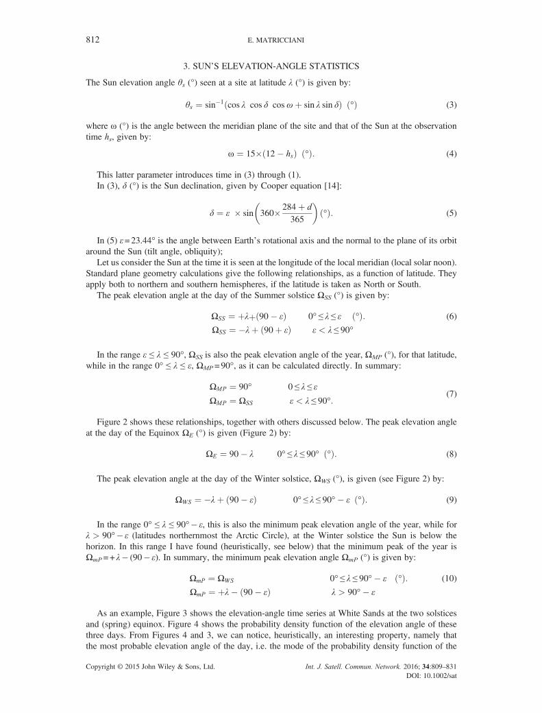
3. SUN’S ELEVATION-ANGLE STATISTICS

The Sun elevation angle θs (°) seen at a site at latitude λ (°) is given by:

θs ¼ sin�1 cos λ cos δ cosωþ sin λ sin δð Þ °ð Þ (3)

where ω (°) is the angle between the meridian plane of the site and that of the Sun at the observationtime hs, given by:

ω ¼ 15� 12� hsð Þ °ð Þ: (4)

This latter parameter introduces time in (3) through (1).In (3), δ (°) is the Sun declination, given by Cooper equation [14]:

δ ¼ ε � sin 360� 284þ d365

� �°ð Þ: (5)

In (5) ε=23.44° is the angle between Earth’s rotational axis and the normal to the plane of its orbitaround the Sun (tilt angle, obliquity);

Let us consider the Sun at the time it is seen at the longitude of the local meridian (local solar noon).Standard plane geometry calculations give the following relationships, as a function of latitude. Theyapply both to northern and southern hemispheres, if the latitude is taken as North or South.

The peak elevation angle at the day of the Summer solstice ΩSS (°) is given by:

ΩSS ¼ þλþ 90� εð Þ 0° ≤ λ ≤ ε °ð Þ:ΩSS ¼ �λþ 90þ εð Þ ε < λ ≤ 90°

(6)

In the range ε ≤ λ ≤ 90°, ΩSS is also the peak elevation angle of the year, ΩMP (°), for that latitude,while in the range 0° ≤ λ ≤ ε, ΩMP=90°, as it can be calculated directly. In summary:

ΩMP ¼ 90° 0 ≤ λ ≤ εΩMP ¼ ΩSS ε < λ ≤ 90°:

(7)

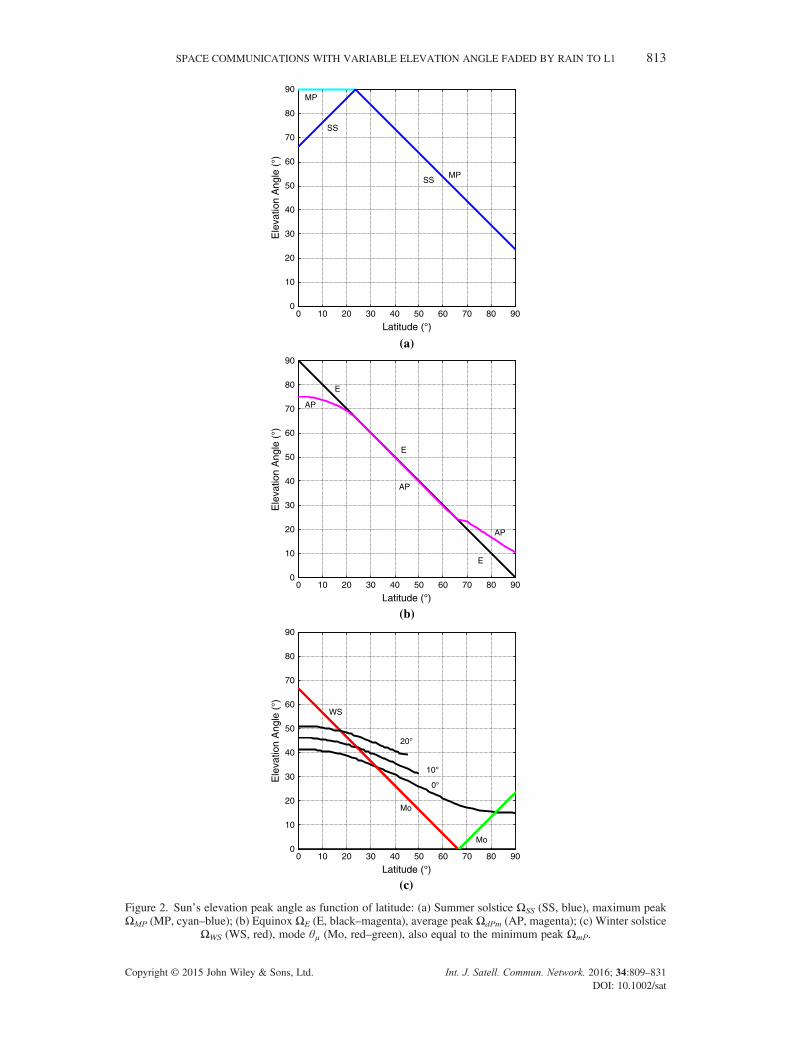
Figure 2 shows these relationships, together with others discussed below. The peak elevation angleat the day of the Equinox ΩE (°) is given (Figure 2) by:

ΩE ¼ 90� λ 0° ≤ λ ≤ 90° °ð Þ: (8)

The peak elevation angle at the day of the Winter solstice, ΩWS (°), is given (see Figure 2) by:

ΩWS ¼ �λþ 90� εð Þ 0° ≤ λ ≤ 90°� ε °ð Þ: (9)

In the range 0° ≤ λ ≤ 90°� ε, this is also the minimum peak elevation angle of the year, while forλ > 90°� ε (latitudes northernmost the Arctic Circle), at the Winter solstice the Sun is below thehorizon. In this range I have found (heuristically, see below) that the minimum peak of the year isΩmP=+ λ� (90� ε). In summary, the minimum peak elevation angle ΩmP (°) is given by:

ΩmP ¼ ΩWS 0° ≤ λ ≤ 90°� ε °ð Þ:ΩmP ¼ þλ� 90� εð Þ λ > 90°� ε

(10)

As an example, Figure 3 shows the elevation-angle time series at White Sands at the two solsticesand (spring) equinox. Figure 4 shows the probability density function of the elevation angle of thesethree days. From Figures 4 and 3, we can notice, heuristically, an interesting property, namely thatthe most probable elevation angle of the day, i.e. the mode of the probability density function of the


0 10 20 30 40 50 60 70 80 900

10

20

30

40

50

60

70

80

90

Latitude (°)

Ele

vatio

n A

ngle

(°)

MP

MP

SS

SS

(a)

0 10 20 30 40 50 60 70 80 900

10

20

30

40

50

60

70

80

90

Latitude (°)

Ele

vatio

n A

ngle

(°)

0 10 20 30 40 50 60 70 80 900

10

20

30

40

50

60

70

80

90

Latitude (°)

Ele

vatio

n A

ngle

(°)

AP

AP

AP

E

E

E

(b)

(c)

0°

10°

20°

Mo

Mo

WS

Figure 2. Sun’s elevation peak angle as function of latitude: (a) Summer solstice ΩSS (SS, blue), maximum peakΩMP (MP, cyan–blue); (b) Equinox ΩE (E, black–magenta), average peak ΩdPm (AP, magenta); (c) Winter solstice

ΩWS (WS, red), mode θμ (Mo, red–green), also equal to the minimum peak ΩmP.



5 10 15 200

10

20

30

40

50

60

70

80

90

Clock Time (h)

Sun

Ele

vatio

n A

ngle

(°)

White Sands

WS

SS

E

Figure 3. Elevation-angle time series at the two solstices (WS: Winter; SS: Summer) and Spring equinox (E),White Sands (λ= 32.54 °N). Notice that the time scale is the clock (civil) time, not the solar time (the two differ

according to (1)).

0 10 20 30 40 50 60 70 80 900

0.1

0.2

0.3

0.4

0.5

0.6

0.7

0.8

0.9

1

Angle (°)

Nor

mal

ized

Pro

babi

lity

Den

sity

White Sands

SSWS E

Figure 4. Normalized probability density function of the elevation angle of the Sun (L1), White Sands (λ=32.54 °N),at the Summer solstice (SS), Winter solstice (WS) and the equinox (E). For the purpose of clearly comparing the

peaks, the densities are normalized to their peak (mode); therefore their integrals differ from one.

814 E. MATRICCIANI

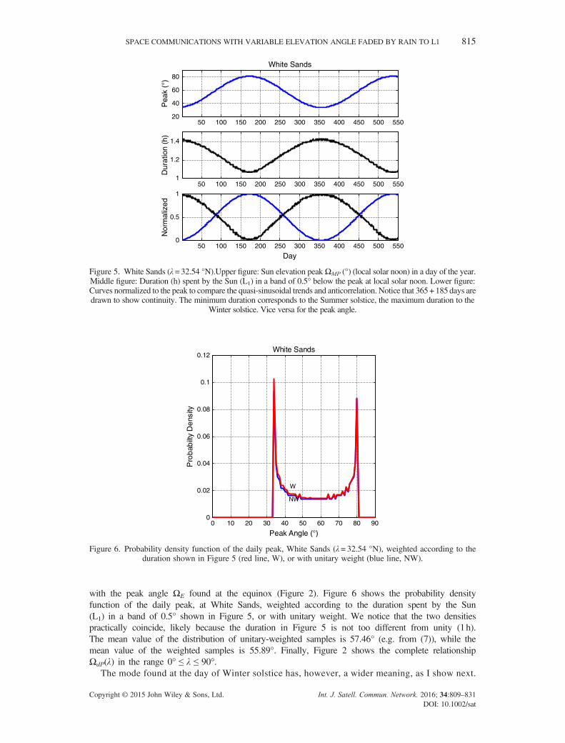
day (the peak in Figure 4), θμ (°), always coincides with the peak angle of that day (Figure 3). That thetwo angles coincide can be deduced from the time series shown in Figure 3: near the peak the rate ofchange of the Sun’s elevation angle decreases down to zero, therefore θs(t) spends more time in an am-plitude band Δθs around the peak than around any other value in the same band. Figure 5 shows howthe daily peak, ΩdP (°), changes in a year and also the time the Sun spends in an amplitude bandΔθs=0.5° just below the peak. In conclusion, in any day of the year the mode (i.e. the most probablevalue) and the peak coincide; therefore the mode is determined by the Sun–Earth orbit.

Moreover, a study of the statistics of the daily peak shown in Figure 5, each peak weighted identically(1 sample per day), shows, heuristically, that the mean value of ΩdP, ΩdPm (°), always coincides in therange ε ≤ λ ≤ 90� ε (Tropic of Cancer to the Arctic Circle, or Tropic of Capricorn to the Antarctic Circle)


50 100 150 200 250 300 350 400 450 500 55020

40

60

80

Pea

k (°

)

White Sands

50 100 150 200 250 300 350 400 450 500 5501

1.2

1.4

Dur

atio

n (h

)

50 100 150 200 250 300 350 400 450 500 5500

0.5

1

Day

Nor

mal

ized

Figure 5. White Sands (λ=32.54 °N).Upper figure: Sun elevation peakΩMP (°) (local solar noon) in a day of the year.Middle figure: Duration (h) spent by the Sun (L1) in a band of 0.5° below the peak at local solar noon. Lower figure:Curves normalized to the peak to compare the quasi-sinusoidal trends and anticorrelation. Notice that 365+185days aredrawn to show continuity. The minimum duration corresponds to the Summer solstice, the maximum duration to the

Winter solstice. Vice versa for the peak angle.

0 10 20 30 40 50 60 70 80 900

0.02

0.04

0.06

0.08

0.1

0.12

Pro

babi

lty D

ensi

ty

Peak Angle (°)

White Sands

W

NW

Figure 6. Probability density function of the daily peak, White Sands (λ= 32.54 °N), weighted according to theduration shown in Figure 5 (red line, W), or with unitary weight (blue line, NW).


with the peak angle ΩE found at the equinox (Figure 2). Figure 6 shows the probability densityfunction of the daily peak, at White Sands, weighted according to the duration spent by the Sun(L1) in a band of 0.5° shown in Figure 5, or with unitary weight. We notice that the two densitiespractically coincide, likely because the duration in Figure 5 is not too different from unity (1h).The mean value of the distribution of unitary-weighted samples is 57.46° (e.g. from (7)), while themean value of the weighted samples is 55.89°. Finally, Figure 2 shows the complete relationshipΩdP(λ) in the range 0° ≤ λ ≤ 90°.

The mode found at the day of Winter solstice has, however, a wider meaning, as I show next.


816 E. MATRICCIANI

Let us study the probability density function of θs in a year, conditioned to the minimum elevation angleof observation. As an example, Figure 7 shows the density functions found at White Sands for differentminimum elevation angle θmin=0°, 5°, 10°, 20°. It clearly shows that the mode is a function only of thelatitude. Therefore, in general, Figure 8 shows how the density function varies with latitude for θmin=0°.

A detailed study of the relationship between mode and latitude (as in Figure 8) is, at first sight, a littlesurprising. In fact, I have found that in the range 0° ≤ λ ≤ 90°� ε, the mode coincides with the peakfound at the same latitude at the Winter solstice, ΩWS, thus confirming the link to the Sun–planet orbit.This coincidence is likely because of the fact, already observed, that in any day of the year the mode andthe peak coincide. Now, heuristically, when all data of the year are considered in a single probabilitydensity function, we can observe (see Figure 3) that in every day of the year any two symmetrical ele-vation angles below the Winter solstice peak are always sampled, while all other symmetrical anglesaround the peak of a day occur less frequently, as we approach the summer solstice, and that the longer

0 10 20 30 40 50 60 70 80 900

0.005

0.01

0.015

0.02

0.025

0.03

0.035

Angle (°)

Pro

babi

lity

Den

sity

White Sands

0°

5°

10°

20°

Figure 7. Probability density function of the elevation angle of the Sun (L1), White Sands (λ= 32.54 °N), in ayear, for different minimum elevation angles (0°, black; 5°, magenta; 10°, blue; 20°, red).

0 10 20 30 40 50 60 70 80 900

0.1

0.2

0.3

0.4

0.5

0.6

0.7

0.8

0.9

1

Angle (°)

Nor

mal

ized

Pro

babi

lity

Den

sity

23.44° Lat=0°66.56° 90°80°

Figure 8. Probability density function of the elevation angle of the Sun (L1) at latitude λ= 0° (red), λ = ε (black),λ= 90°� ε (blue), λ = 80° (cyan), λ= 90° (magenta), in a year. All peak values can be calculated from (7) or

Table II.



interval (amplitude band Δθs) always occurs at the Winter solstice. Besides this heuristic argument Icould not find a mathematical proof in the literature (see Appendix B).

Finally, in the range 90°� ε< λ ≤ 90°, again heuristically, I have found that the mode increases line-arly from 0° to ε. Therefore the overall relationship between the mode θμ(λ) and the latitude λ is given by:

θμ ¼ ΩWS 0 ≤ λ ≤ 90°� ε °ð Þ:θμ ¼ λ� 90� εð Þ 90°� ε < λ ≤ 90°

(11)

In other words, up to the Arctic Circle (Antarctic Circle), the peak elevation angle observed at theWin-ter solstice at a site gives the most probable elevation angle of the Sun in all year, while northernmost(southernmost) the mode increases linearly from 0° to ε. Figure 2 shows also this relationship. We can ex-tend this theorem by stating that, in any continuous period of the year, the mode of the Sun’s elevationangle is given by the minimum daily peak angle of that period. Table II summarizes these relationships.

A similar study conducted on the mean elevation angle, θm (°), as a function of the latitude, derivednow with a best fit (hence an approximate relationship), gives (see the black line for θmin = 0°, Figure 2)the following relationship:

θm ¼ 13:29 cos 2λð Þ þ 28:17 0 ≤ λ ≤ 90° °ð Þ: (12a)

The dependence of θm on θmin can be found in the results shown in Figure 9, up to θmin = 30°,

Table II. Sun’s (L1) elevation-angle θS (°) as a function of latitude λ (°). The relationships are valid both for theNorthern and Southern hemispheres, if the latitude refers to one of the two. Notice that λ= ε is the latitude of

the Tropic Circles, λ = 90°� ε of the Arctic and Antarctic Circles.

Parameter 0° ≤ λ ≤ ε ε< λ ≤ 90°� ε 90� ε ≤ λ ≤ 90°

Summer Solstice Peak ΩSS = + λ + (90� ε) ΩSS=� λ+ (90 + ε) ΩSS =� λ + (90 + ε)Equinox Peak ΩE =� λ+ 90 ΩE=� λ+ 90 ΩE =� λ+ 90Winter Solstice Peak ΩWS =� λ+ (90� ε) ΩWS=� λ + (90� ε) —Maximum Peak ΩMP = 90° ΩMP=ΩSS ΩMP =ΩSSMean Peak (not weighted) See Figure 2 ΩdPm =ΩE See Figure 2Minimum Peak ΩmP =ΩWS ΩmP=ΩWS ΩmP= + λ� (90� ε)Mode θμ =ΩWS θμ =ΩWS θμ = + λ� (90� ε)

0 5 10 15 20 25 30 35 4020

25

30

35

40

45

50

55

60

Minimum Elevation Angle (°)

Ave

rage

Ele

vatio

n A

ngle

( °

)

Lat=0°

23.44°

45°

35°

Figure 9. Average (mean) elevation angle of the Sun, θm (°), as a function of the minimum elevation angle considered,θmin (°). The slope of θm is approximately 5°/decade.


818 E. MATRICCIANI

obtained from the curves shown in Figure 8. As we can notice, the mean value increases approxi-mately 5°/decade of θmin, so that we can write (12a) as:

θm ¼ 13:29 cos 2λð Þ þ 28:17þ 0:5θmin θm ≤ΩMP; θmin < 30° °ð Þ: (12b)

From Figure 2 we can directly establish if the probability density function of θs, at a given lati-tude, is skewed to the right (θm> θμ), or to the left (θm< θμ), for a given θmin. The median value(value exceeded with probability 0.5) is always between the mode and the mean.

4. ELEVATION ANGLE SAMPLING AND RAIN ATTENUATION CALCULATION

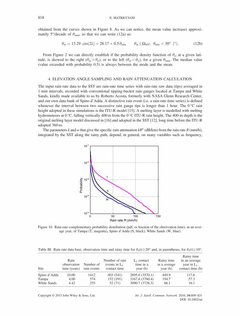
The input rain-rate data to the SST are rain-rate time series with rain-rate raw data (tips) averaged in1-min intervals, recorded with conventional tipping-bucket rain gauges located at Tampa and WhiteSands, kindly made available to us by Roberto Acosta, formerly with NASA Glenn Research Center,and our own data bank of Spino d’Adda. A distinctive rain event (i.e. a rain-rate time series) is definedwhenever the interval between two successive rain gauge tips is longer than 1 hour. The 0 °C rainheight adopted in these simulations is the ITU-R model [15]. A melting layer is modelled with meltinghydrometeors at 0 °C, falling vertically 400m from the 0 °C ITU-R rain height. The 400-m depth is theoriginal melting layer model discussed in [16] and adopted in the SST [12], long time before the ITU-Radopted 360m.

The parameters k and α that give the specific rain attenuation kRα (dB/km) from the rain rate R (mm/h),integrated by the SST along the rainy path, depend, in general, on many variables such as frequency,

0 50 100 15010-5

10-4

10-3

10-2

10-1

Rain rate R (mm/h)

Pro

babi

lity

S

W

T

Figure 10. Rain-rate complementary probability distribution (pdf, or fraction of the observation time), in an aver-age year, of Tampa (T, magenta), Spino d’Adda (S, black), White Sands (W, blue).

Table III. Rain rate data base, observation time and rainy time for θS(t) ≥ 20° and, in parentheses, for θS(t) ≥ 10°.

Site

Rainobservationtime (years)

Number ofrain events

Number of rainevents in L1

contact time

L1 contacttime in ayear (h)

Rainy timein a averageyear (h)

Rainy timein an averageyear in L1

contact time (h)

Spino d’Adda 10.00 1412 403 (541) 2695.0 (3570.1) 449.9 117.6Tampa 4.00 574 152 (191) 3167.6 (3760.4) 194.7 57.3White Sands 4.42 255 52 (71) 3090.7 (3726.3) 66.1 16.1



polarization, elevation angle, drop-size distribution, water temperature, time. For long-term studies andpredictions, we adopt values of k and α that depend only on polarization (assumed circular in this paper)and temperature, once a drop-size distribution is assumed, such as those reported in [17] at 0 °C and 20 °C,useful for modelling the melting layer and the rain layer [12, 16].We have adopted these constants, both inthis work and in the previous studies with the SST because they provide a consistent and reliable set ofdata at 0 °C and 20°C water temperatures.

Figure 10 shows the rain-rate complementary probability distribution functions exceeded in an av-erage year. These are the unconditional input pdf to all prediction methods that predict rain-attenuationpdf for long-term continuous observation time (e.g. for Earth orbits), not for a spacecraft contact time,which needs conditional statistics. We show them because large differences can be noted in the rainrate of the sites, and also because they are used by the SST at zenith paths. Other important differences,such as the number of rainstorms and the rainy time in an average year, are reported in Table III.

5 10 15 20-3

-2

-1

0

1

2

3

Time(h)

Rat

e of

Cha

nge

White Sands Winter Solstice

12 min

3 min

6 min

(a)

5 10 15 20-3

-2

-1

0

1

2

3

Time(h)

Rat

e of

Cha

nge

(b)

White Sands Summer Solstice

6 min

3 min

12 min

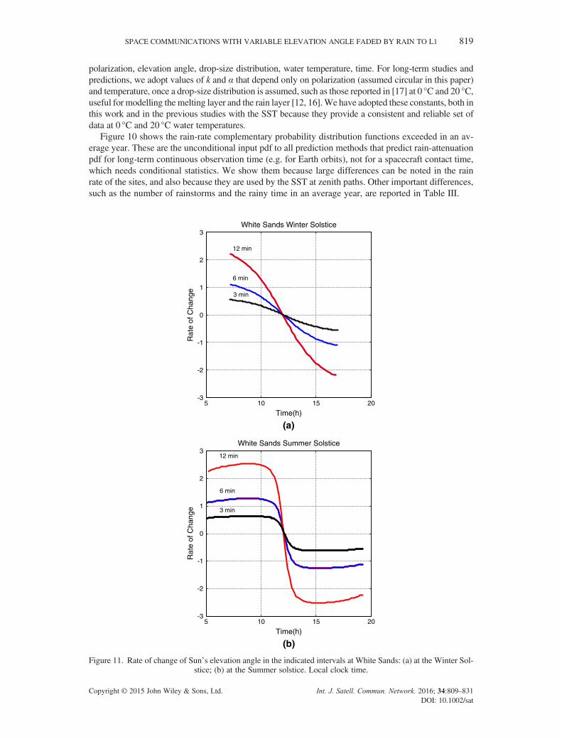
Figure 11. Rate of change of Sun’s elevation angle in the indicated intervals at White Sands: (a) at the Winter Sol-stice; (b) at the Summer solstice. Local clock time.


820 E. MATRICCIANI

The SST was developed for calculating rain-attenuation time series in terrestrial or fixed slantpaths, i.e. paths with constant elevation angle [12]. To estimate rain attenuation in a link to L1,we have to apply the SST to a path with changing elevation angle. To achieve this goal, firstwe need to sample the Sun elevation angle θs(t)≥ θmin, and keep it constant for an interval of timein which the elevation angle does not change too much for rain attenuation calculations (tenths ofdB). Notice that by using (3) we neglect the effects of the atmosphere because rain attenuation isinsensitive to small changes of the angle of arrival of the electromagnetic wave (i.e. ray bendingand defocusing).

In other words, for each interval of sampling time and corresponding elevation angle found at thebeginning of the interval, the SST transforms the complete rain-rate time series of the event occurringat that time into a rain-attenuation time series calculated with that elevation angle (the elevation angleaffects the speed of rainstorm along the slant path, which becomes infinite at zenith, see [12]). Thecomplete rain-attenuation time series, i.e. the one that simulates the rain-attenuation time series thatwould be measured in the path with a continuously changing elevation angle θs(t)≥ θmin, is thenobtained by adding all the non-overlapping (disjoint) pieces of rain-attenuation time series found ineach interval, therefore obtaining a continuous rain-attenuation time series whose elevation anglechanges in small steps, within the contact time of the day.

I have assessed empirically the length of such a fixed interval by studying the sensitivity of the longterm rain-attenuation pdf to the interval length, and have found that 6min is a good compromise, in anyday of the year, between the need to describe rain attenuation with sufficient accuracy and the need toprocess a manageable number of rain-attenuation time series at constant elevation angle for each rain-rate time series.

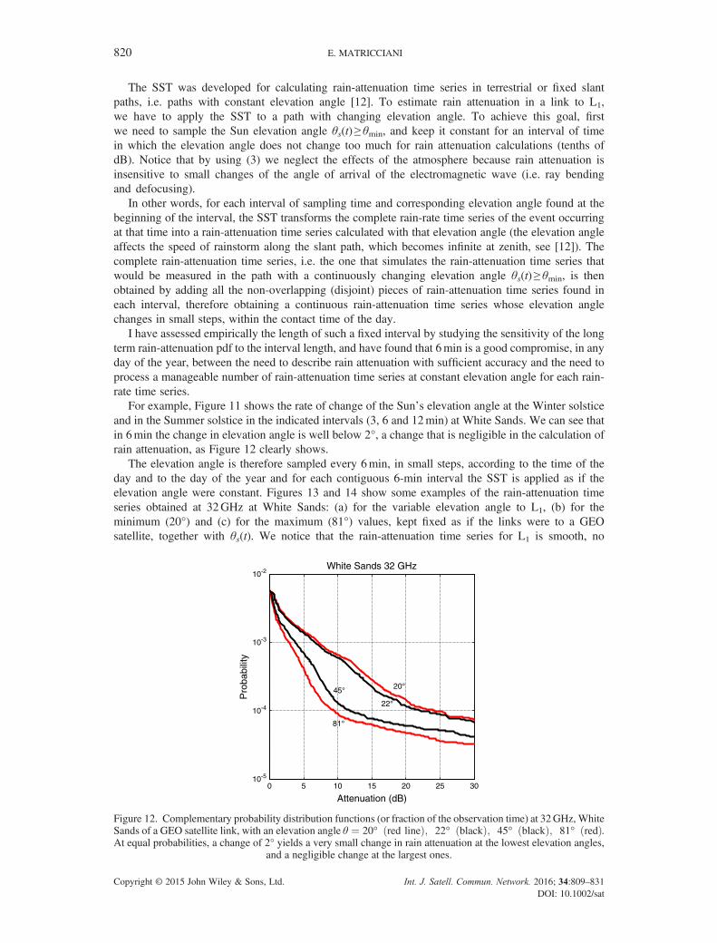
For example, Figure 11 shows the rate of change of the Sun’s elevation angle at the Winter solsticeand in the Summer solstice in the indicated intervals (3, 6 and 12min) at White Sands. We can see thatin 6min the change in elevation angle is well below 2°, a change that is negligible in the calculation ofrain attenuation, as Figure 12 clearly shows.

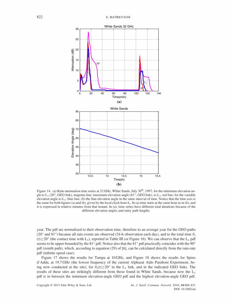
The elevation angle is therefore sampled every 6min, in small steps, according to the time of theday and to the day of the year and for each contiguous 6-min interval the SST is applied as if theelevation angle were constant. Figures 13 and 14 show some examples of the rain-attenuation timeseries obtained at 32GHz at White Sands: (a) for the variable elevation angle to L1, (b) for theminimum (20°) and (c) for the maximum (81°) values, kept fixed as if the links were to a GEOsatellite, together with θs(t). We notice that the rain-attenuation time series for L1 is smooth, no

0 5 10 15 20 25 3010-5

10-4

10-3

10-2White Sands 32 GHz

Attenuation (dB)

Pro

babi

lity

20°

22°

81°

45°

Figure 12. Complementary probability distribution functions (or fraction of the observation time) at 32GHz, WhiteSands of a GEO satellite link, with an elevation angle θ ¼ 20° red lineð Þ; 22° blackð Þ; 45° blackð Þ; 81° redð Þ.At equal probabilities, a change of 2° yields a very small change in rain attenuation at the lowest elevation angles,

and a negligible change at the largest ones.


0 20 40 60 80 100 120 140 160 180 2000

20

40

60

80

100

120

140

Time(min)

Atte

nuat

ion

(dB

)

White Sands 32 GHz

20°

81°

L1

(a)

11.5 12 12.5 13 13.5 14 14.520

30

40

50

60

70

80

90

Time(h)

Ele

vatio

n A

ngle

(de

g)

White Sands

(b)

Figure 13. (a) Rain-attenuation time series at 32GHz, White Sands, July 15th, 1996, for the minimum elevation an-gle to L1 (20°, GEO link), magenta line (the high value of the peak attenuation is because of the long path length,that the SST assumes completely filled with rain); maximum elevation angle (81°, GEO link), red line; for the variableelevation angle to L1, blue line; (b) the Sun elevation angle in the same interval of time. Notice that the time axis is thesame for both figures (a) and (b), given by the local clock hour hc. In (a) time starts at the same hour as in (b), and it isexpressed in relative minutes from that instant. In (a), time series have different total durations because of the different

elevation angles and rainy path lengths.


appreciable discontinuity is present and so I have been reassured that the 6-min sampling time iseffective for the purpose.

It is obvious that the possible contact time with a deep-space probe at L1 is less in winter than insummer (see Figure 3), and this fact will select particular rain events during the daylight, whose occur-rence depends on site climate.

5. RAIN ATTENUATION STATISTICAL RESULTS

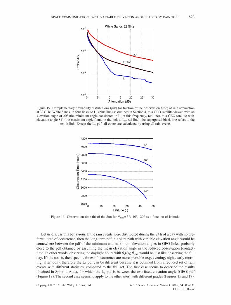
I report several rain attenuation statistical results with interesting features. Figure 15 shows the rain at-tenuation pdf at 32GHz, for White Sands, in three cases: the link to L1 as described in Section 4 duringthe contact time, the link to a GEO satellite viewed with an elevation angle 20° (the minimum angle con-sidered to L1), or 81° (the maximum angle found at White Sands in the link to L1) during an average


0 20 40 60 80 100 120 1400

5

10

15

20

25

30

Time(min)

Atte

nuat

ion

(dB

)

White Sands 32 GHz

20°

81°

L1

(a)

13.5 14 14.5 15 15.520

30

40

50

60

70

80

90

Time(h)

Ele

vatio

n A

ngle

(de

g)

White Sands

(b)

Figure 14. (a) Rain-attenuation time series at 32GHz, White Sands, July 30th, 1997, for the minimum elevation an-gle to L1 (20°, GEO link), magenta line; maximum elevation angle (81°, GEO link), to L1, red line; for the variableelevation angle to L1, blue line; (b) the Sun elevation angle in the same interval of time. Notice that the time axis isthe same for both figures (a) and (b), given by the local clock hour hc. In (a) time starts at the same hour as in (b), andit is expressed in relative minutes from that instant. In (a), time series have different total durations because of the

different elevation angles and rainy path lengths.

822 E. MATRICCIANI

year. The pdf are normalized to their observation time, therefore to an average year for the GEO paths(20° and 81°) because all rain events are observed (24-h observation each day), and to the total time θs(t)≥ 20° (the contact time with L1), reported in Table III (or Figure 16). We can observe that the L1 pdfseems to be upper-bounded by the 81° pdf. Notice also that the 81° pdf practically coincides with the 90°pdf (zenith path), which, according to equation (29) of [6], can be calculated directly from the rain-ratepdf (infinite speed case).

Figure 17 shows the results for Tampa at 10GHz, and Figure 18 shows the results for Spinod’Adda, at 19.7GHz (the lowest frequency of the current Alphasat Aldo Paraboni Experiment, be-ing now conducted at the site), for θs(t)≥ 20° in the L1 link, and in the indicated GEO links. Theresults of these sites are strikingly different from those found in White Sands, because now the L1

pdf is in between the minimum elevation-angle GEO pdf and the highest elevation-angle GEO pdf.


0 5 10 15 20 25 3010-5

10-4

10-3


Attenuation (dB)

Pro

babi

lity

81°, 90°

20°

L1

Figure 15. Complementary probability distributions (pdf) (or fraction of the observation time) of rain attenuationat 32GHz, White Sands, in four links: to L1 (blue line) as outlined in Section 4, to a GEO satellite viewed with anelevation angle of 20° (the minimum angle considered to L1 at this frequency, red line), to a GEO satellite withelevation angle 81° (the maximum angle found in the link to L1, red line); the superposed black line refers to the

zenith link. Except the L1 pdf, all others are calculated by using all rain events.

0 10 20 30 40 502600

2800

3000

3200

3400

3600

3800

4000

4200

Latitude (°)

Obs

erva

tion

Tim

e (h

ours

)

20°

10°

5°

Figure 16. Observation time (h) of the Sun for θmin = 5°, 10°, 20° as a function of latitude.


Let us discuss this behaviour. If the rain events were distributed during the 24 h of a day with no pre-ferred time of occurrence, then the long-term pdf in a slant path with variable elevation angle would besomewhere between the pdf of the minimum and maximum elevation angles in GEO links, probablyclose to the pdf obtained by assuming the mean elevation angle in the reduced observation (contact)time. In other words, observing the daylight hours with θs(t)≥ θmin would be just like observing the fullday. If it is not so, then specific times of occurrence are more probable (e.g. evening, night, early morn-ing, afternoon); therefore the L1 pdf can be different because it is obtained from a reduced set of rainevents with different statistics, compared to the full set. The first case seems to describe the resultsobtained in Spino d’Adda, for which the L1 pdf is between the two fixed elevation-angle (GEO) pdf(Figure 18). The second case seems to apply to the other sites, with different grades (Figures 15 and 17).


0 5 10 15 20 25 3010-5

10-4

10-3

10-2

10-1Tampa 10 GHz

Attenuation (dB)

Pro

babi

lity

20°

85°

90°

L1

Figure 17. Complementary probability distributions (pdf) (or fraction of the observation time) of rain attenuation at10GHz, Tampa, in four links: to L1 (blue line) as outlined in Section 4, to a GEO satellite viewed with an elevationangle of 20° (the minimum angle considered to L1 at this frequency, red line), to a GEO satellite with elevation angle85° (the maximum angle found in the link to L1, red line); the superposed black line refers to the zenith link. Except

the L1 pdf, all others are calculated by using all rain events.

0 5 10 15 20 25 3010-5

10-4

10-3

10-2

10-1Spino 19.7 GHz

Attenuation (dB)

P(A

)

L1

L120°

90°

68°

Figure 18. Complementary probability distributions (pdf) (or fraction of the observation time) of rain attenuationat 19.7GHz, Spino d’Adda, in four links: to L1 (blue line) as outlined in Section 4, to a GEO satellite viewed withan elevation angle of 20° (the minimum angle considered to L1 at this frequency, red line), to a GEO satellite withelevation angle 68° (the maximum angle found in the link to L1, red line); the superposed black line refers to the

zenith link. Except the L1 pdf, all others are calculated by using all rain events.

824 E. MATRICCIANI

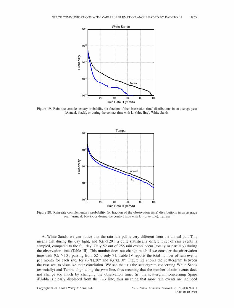
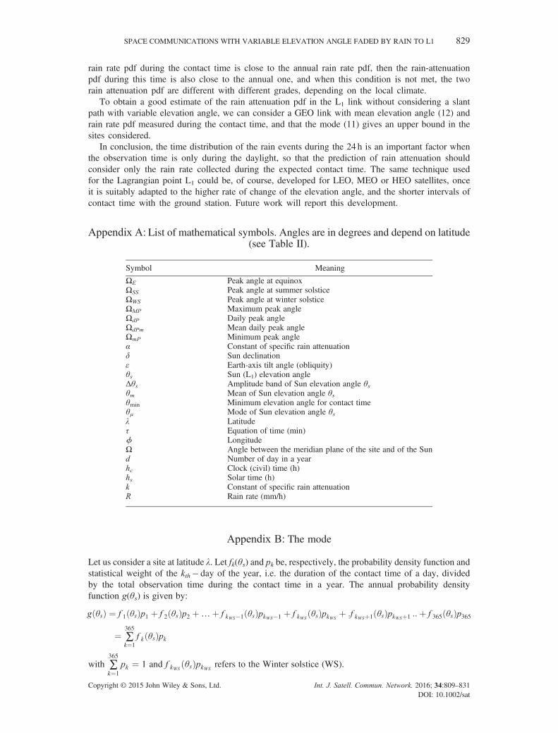
Let us discuss more deeply these results. Figures 19–21 show the rain rate pdf exceeded in anaverage year and in the observation time to L1 with θs(t)≥ 20°. As before for rain attenuation pdf, alsothese pdf are normalized to the observation time, therefore to an average year for the annual pdf, and tothe total time θs(t)≥ 20° for the links to L1.


0 20 40 60 80 10010-5

10-4

10-3

10-2

10-1

Rain Rate R (mm/h)

Pro

babi

lity

White Sands

AnnualL1

Figure 19. Rain-rate complementary probability (or fraction of the observation time) distributions in an average year(Annual, black), or during the contact time with L1 (blue line), White Sands.

0 20 40 60 80 10010-5

10-4

10-3

10-2

10-1

Rain Rate R (mm/h)

Pro

babi

lity

Tampa

L1

Annual

Figure 20. Rain-rate complementary probability (or fraction of the observation time) distributions in an averageyear (Annual, black), or during the contact time with L1 (blue line), Tampa.


At White Sands, we can notice that the rain rate pdf is very different from the annual pdf. Thismeans that during the day light, and θs(t)≥ 20°, a quite statistically different set of rain events issampled, compared to the full day. Only 52 out of 255 rain events occur (totally or partially) duringthe observation time (Table III). This number does not change much if we consider the observationtime with θs(t)≥ 10°, passing from 52 to only 71. Table IV reports the total number of rain eventsper month for each site, for θs(t)≥ 20° and θs(t)≥ 10°. Figure 22 shows the scattergram betweenthe two sets to visualize their correlation. We see that: (i) the scattergram concerning White Sands(especially) and Tampa align along the y= x line, thus meaning that the number of rain events doesnot change too much by changing the observation time; (ii) the scattergram concerning Spinod’Adda is clearly displaced from the y= x line, thus meaning that more rain events are included


Figure 21. Rain-rate complementary probability (or fraction of the observation time) distributions in an averageyear (Annual, black), or during the contact time with L1 (blue line), Spino d’Adda.

Table IV. Total number of rain events per month (1–12), for each site in the L1 contact time of Table III, accordingto the minimum elevation angle: θS(t) ≥ 20° (first line), θS(t) ≥ 10° (second line).

Site 1 2 3 4 5 6 7 8 9 10 11 12

Spino d’Adda 13 10 31 52 68 49 37 37 45 27 26 830 17 39 63 75 56 46 48 55 39 45 28

Tampa 10 8 7 14 10 14 18 23 21 9 5 1311 9 8 15 14 16 28 32 25 13 5 15

White Sands 2 4 1 2 0 2 9 9 5 7 6 54 6 1 2 0 4 13 10 6 8 9 8

Figure 22. Scattergram between the total number NR of rain events considered in the L1 pdf, for θs(t) ≥ 20°(abscissa) and θs(t) ≥ 10° (ordinate), for each month of the year. Spino d’Adda (black circles); Tampa (magenta

diamonds); White Sands (blue triangles).

826 E. MATRICCIANI



by increasing the observation time. In other words, the sampling of rain events depends on site andminimum elevation angle; therefore it must affect rain attenuation statistics, as we see next.

Figures 23–25 show the rain attenuation pdf calculated in the link to L1 by using the SST asdescribed in Section 4, and that calculated: (i) in a slant path with fixed elevation angle (a GEO link)with elevation angle equal either to the mean elevation angle during the contact time with θs(t)≥ 20°(see (12b)), or equal to the mode (see (11)), with the rain rate pdf of the contact time; (ii) by usingthe SST in a GEO link with elevation angle equal to the mean elevation angle, as in (i), but with therain rate pdf of an average year.

0 5 10 15 20 25 3010-5

10-4

10-3


Attenuation (dB)

Pro

babi

lity

L1

43.8° L1

43.8° Annual

34°

Figure 23. Complementary probability distributions (or fraction of the observation time) at 32GHz, White Sands:to L1 (blue line), to a GEO satellite viewed with an elevation angle θm = 43.8° (lower black line, L1), θμ = 34° (redline), by using only the rain events during the contact time, and θm= 43.8° (upper black line, Annual) by using all

rain events.

0 5 10 15 20 25 3010-5

10-4

10-3

10-2

10-1Tampa 10 GHz

Attenuation (dB)

Pro

babi

lity

L1

45.8°

45.8°L1

Annual

38.9°

Figure 24. Complementary probability (or fraction of the observation time) distributions at 10GHz, Tampa: to L1

(blue line), to a GEO satellite viewed with an elevation angle θm= 45.8° (lower black line, L1), θμ = 38.9°, (red line),by using only the rain events during the contact time, and θm= 45.8° (upper black line, Annual) by using all rain

events.


0 5 10 15 20 25 3010-5

10-4

10-3

10-2

10-1 Spino 19.7 GHz

Attenuation (dB)

Pro

babi

lity

L1

21.2°38°L1

38°Annual

Figure 25. Complementary probability (or fraction of the observation time) distributions at 19.7GHz, Spino d’Adda:to L1 (blue line), to a GEO satellite viewed with an elevation angle θm=38.0° (lower black line, L1), θμ =21.2°, (redline), by using only the rain events during the contact time, and θm=38.0° (magenta line, Annual) by using all

rain events.

828 E. MATRICCIANI

The comparison between the rain attenuation pdf calculated with the rain rate pdf measured onlyduring the observation (contact) time θs(t)≥ 20° and that measured with the annual rain rate pdf isstraightforward: when the two rain rate pdf are quite different (sampling does affect rain observation),as in White Sands, the two rain attenuation pdf are very different. When the two rain rate pdf are aboutthe same (sampling does not affect rain observation), the two rain attenuation pdf are very alike, as inTampa and Spino d’Adda, with different grade. Finally, notice that if the mode (11) is assumed in theGEO link, the rain attenuation pdf, at these latitudes (the mode is smaller than the mean with θm=20°,see Figure 2), is an upper bound to all predictions.

6. CONCLUSIONS

I have investigated how rain attenuation changes in slant paths with variable elevation angles, by sim-ulating rain-attenuation time series with the Synthetic Storm Technique (SST), applied to radio links toa spacecraft located at the Sun–Earth first Lagrangian point L1, viewed from three ground sites withdifferent meteorological conditions (Spino d’Adda, Tampa, White Sands, Table I). To a first approxi-mation, the results reported can be also applied to communications with spacecrafts orbiting Mercury,such as the ESA Mercury Planetary Orbiter and the Mercury Magnetospheric Orbiter, both on boardthe ESA Bepi Colombo spacecraft, because this planet, as seen from the Earth, is angularly close tothe Sun.

First, I have summarized known results on the elevation angle of the Sun, θs (°), seen at site atlatitude λ (°), but I have also found what seems to be a new and interesting result, namely that themost probable value of θs (the mode of the probability density function of θs in a year) is given by(11), therefore linked to the Sun–planet orbit. Figure 2 shows all the results concerning θs(λ), andTable II summarizes the corresponding formulae. These relationships are also valid for the elevationangle of the Sun seen from other planets, for example Mars, by assuming, in this case, the tilt angleε=25.19°.

Second, I have calculated rain-attenuation time series with the SST. The results show that thecomplementary probability distribution function (pdf) of rain attenuation in the slant path to L1,compared to GEO pdf calculated with several elevation angles at the same site, depends on therain-rate pdf during the contact time with L1, i.e. during the daylight with θs(t)>20°. When the



rain rate pdf during the contact time is close to the annual rain rate pdf, then the rain-attenuationpdf during this time is also close to the annual one, and when this condition is not met, the tworain attenuation pdf are different with different grades, depending on the local climate.

To obtain a good estimate of the rain attenuation pdf in the L1 link without considering a slantpath with variable elevation angle, we can consider a GEO link with mean elevation angle (12) andrain rate pdf measured during the contact time, and that the mode (11) gives an upper bound in thesites considered.

In conclusion, the time distribution of the rain events during the 24 h is an important factor whenthe observation time is only during the daylight, so that the prediction of rain attenuation shouldconsider only the rain rate collected during the expected contact time. The same technique usedfor the Lagrangian point L1 could be, of course, developed for LEO, MEO or HEO satellites, onceit is suitably adapted to the higher rate of change of the elevation angle, and the shorter intervals ofcontact time with the ground station. Future work will report this development.

Appendix A: List of mathematical symbols. Angles are in degrees and depend on latitude(see Table II).

Symbol Meaning

ΩE Peak angle at equinoxΩSS Peak angle at summer solsticeΩWS Peak angle at winter solsticeΩMP Maximum peak angleΩdP Daily peak angleΩdPm Mean daily peak angleΩmP Minimum peak angleα Constant of specific rain attenuationδ Sun declinationε Earth-axis tilt angle (obliquity)θs Sun (L1) elevation angleΔθs Amplitude band of Sun elevation angle θsθm Mean of Sun elevation angle θsθmin Minimum elevation angle for contact timeθμ Mode of Sun elevation angle θsλ Latitudeτ Equation of time (min)ϕ LongitudeΩ Angle between the meridian plane of the site and of the Sund Number of day in a yearhc Clock (civil) time (h)hs Solar time (h)k Constant of specific rain attenuationR Rain rate (mm/h)

Appendix B: The mode

Let us consider a site at latitude λ. Let fk(θs) and pk be, respectively, the probability density function andstatistical weight of the kth� day of the year, i.e. the duration of the contact time of a day, dividedby the total observation time during the contact time in a year. The annual probability densityfunction g(θs) is given by:

g θsð Þ ¼ f 1 θsð Þp1 þ f 2 θsð Þp2 þ…þ f kWS�1 θsð ÞpkWS�1 þ f kWSθsð ÞpkWS

þ :f kWSþ1 θsð ÞpkWSþ1 ::þ f 365 θsð Þp365

¼ ∑365

k¼1f k θsð Þpk

with ∑365

k¼1pk ¼ 1 and f kWS

θsð ÞpkWSrefers to the Winter solstice (WS).


830 E. MATRICCIANI

Because each density shows a single maximum, taking the derivative of g(θs), the mode θμ is thesolution of the equation:

g’ θsð Þ ¼ ∑365

k¼1f k’ θsð Þpk ¼ 0:

A mathematical proof should prove that:

f 1’ θμ� �

p1 þ f 2’ θμ� �

p2 þ…þ f ’kWS�1 θμ� �

pkWS�1 þ f ’kWSθμ� �

pkWSþ f ’kWSþ1 θμ

� �pkWSþ1 þ…

þf 365’ θμ� �

θμ� �

p365 ¼ f ’kWSθμ� �

pkWS¼ 0

Or, equivalently:

f 1’ θμ� �

p1 þ f 2’ θμ� �

p2…þ f ’kWS�1 θμ� �

pkWS�1 þ f ’kWSþ1 θμ� �

pkWSþ1 þ…þ f 365’ θμ� �

p365 ¼ 0

ACKNOWLEDGEMENTS

The Author wishes to thank Roberto Acosta, formerly with NASA Glenn Research Center, Cleveland (Ohio),for providing the rain-rate raw data of Tampa and White Sands, and Doriana Giammusso and NicolaPignatelli, Engineering Telecommunications students at Politecnico di Milano, for developing some basicsoftware tools used in the study.

REFERENCES

1. Wilson RW. Sun tracker measurements of rain attenuation at 16 and 30 GHz. Bell Syst Tech J 1969; 48:1383–1404.2. Davies PG, Lane JA. Statistics of tropospheric attenuation at 190GHz from observations of solar noise. Electron Lett 1970;

6:522–523.3. Wrixon GT. Measurements of atmospheric attenuation on an Earth–space path at 90 GHZ using a sun tracker. Bell Syst Tech

J 1971:103–114.4. Davies PG. Radiometer measurements of atmospheric attenuation at 19 and 37 GHz along Sun–Earth paths. Proc IEE 1973;

120:159–164.5. Lin SH, Bergmann HJ, Pursley MV. Rain attenuation on Earth–satellite paths—summary of 10 year experiments and stud-

ies. Bell Syst Tech J 1980; 59:183–228.6. Akeyama A, Morita K, Inoue T, Kikushima M. Sasakio, 11- and 18-GHz radio wave attenuation due to precipitation on a

slant path. IEEE Trans Antennas Propag 1980; 28:580–585.7. Davies PG, Mackenzie EC. Review of SHF and EHF slant path propagation measurements made near Slough (UK). IEE

Proc 1981; 128:53–65.8. International Telecommunication Union. Recommendation ITU-R P618-11 Propagation data and prediction methods for the

design of Earth–space telecommunication systems, 2013, P Series Radiowave Propagation.9. Roselló J, Martellucci A, Acosta R, Nessel J, Bråten LE, Riva C. 26-GHz data downlink for LEO satellites, 6th European

Conference on Antennas & Propagation, EuCAP 2012, 111–115, 26–30 March 2012, Prague.10. Liu W, Michelson D. Fade slope analysis of Ka-band Earth–LEO satellite links using a synthetic rain field model. IEEE

Trans Veh Technol 2009; 58:4013–4022.11. Kourogiorgas CI, Panagopoulos AD. A rain attenuation stochastic dynamic model for LEO satellite systems above 10 GHz.

IEEE Trans Veh Technol 2015; 64:829–834.12. Matricciani E. Physical–mathematical model of the dynamics of rain attenuation based on rain rate time series and two layer

vertical structure of precipitation. Radio Sci 1996; 31:281–295.13. Meeus J. Astronomical Algorithms. Willmann-Bell, Richmond: Virginia, 1991.14. Cooper PI. The absorption of radiation in solar stills. Solar Energy 1969; 12:333–346.15. ITU-R Rain height model for prediction methods, ITU-R P series recommendations—radiowave propagation. Long-term

Ka/Ku-band slant path rain attenuation and rain rate statistics. P.839–3, 2001, Geneva.16. Matricciani E. Rain attenuation predicted with a two-layer rain model. Eur Transac Telecommun 1991; 2:715–727.17. Maggiori M. Computed transmission through rain in the 1–400 GHz frequency range for spherical and elliptical drops and

any polarization. Alta Frequenza 1981; 50:262–273.



AUTHOR’S BIOGRAPHY

Copyright © 2015 John Wi

Emilio Matricciani was born in Italy, in 1952. After serving in the Italian Army, hereceived the Laurea degree in Electronics Engineering at Politecnico di Milano, Milan,Italy, in 1978. He joined Politecnico di Milano in 1978 with a research scholarship,and in 1981 he became assistant professor of Electrical Communications. In 1987, hejoined Università di Padova, Padua, Italy, as associate professor of Microwaves. In2001, he qualified as full professor of Telecommunications. Since 1991, he has beenworking with Politecnico di Milano, as professor of Telecommunications. His researchinterests include satellite communications for fixed and mobile systems, deep-spacecommunications, radio propagation at millimetre waves, rain effects on satellite systemdesign and history of science. Most of his early experimental and theoretical activitiesconcerned the propagation and communication experiments devised at Politecnicodi Milano by Francesco Carassa and Aldo Paraboni (satellites SIRIO, ITALSAT and

ALPHASAT Aldo Paraboni experiment). In the ’90s and in the 2000s, he has conducted extensive researchon communications with mobile terminals running in the rain and linked to satellites in the geostationaryorbits, or in lower orbits, and on developing rain attenuation prediction models useful to predict first order(probability distribution functions) and second order (fade durations, rates of change and unavailability duringthe time of the day) statistics for satellite systems design, such as the Synthetic Storm Technique. In additionto the institutional activities, such as lectures on Terrestrial and Satellites Radio Relays, he teaches ScientificWriting to PhD students at Politecnico di Milano and in other Italian Universities.

ley & Sons, Ltd. Int. J. Satell. Commun. Network. 2016; 34:809–831DOI: 10.1002/sat

space communications with variable elevation angle faded

Documents