Space Plasma Physics at the University of Minnesota

Faculty: Cindy Cattell, Bob Lysak, John Wygant, Paul Kellogg (emeritus)

Research Scientists: Yan Song, John Dombeck

Recent Graduates: Jim Crumley (St. John’s University), John Dombeck (University of Minnesota, AGU Scarf Award winner), Mike Johnson (Seagate), Andreas Keiling (UC Berkeley), Doug Rowland (NASA Goddard), Kris Sigsbee (U. of Iowa),

Research focus: Study of the plasmas in the Earth’s magnetosphere and interplanetary space: Aurora, Radiation Belts, Magnetic Reconnection, Field-Aligned Current Generation, Particle Acceleration, Waves: 1 mHz to 1 MHz

Space Plasma PhysicsPlasmas: Low-density gas of charged particles exhibiting collective behavior

Collective behavior: Charged particles in a plasma interact more strongly with long-range fields produced by all other particles rather than two particle collisions

How we study plasmas in space: Satellite and sounding rocket missions instrumented with electric and magnetic field detectors, energetic particle detectors, visible imagers to see aurora, etc.

Current Missions: Fast Auroral Snapshot (FAST), Polar, Wind, Ulysses, Geotail, CRRES, Cluster, STEREO, Themis

Upcoming Mission: Radiation Belt Storm Probe (launch planned 2012): John Wygant, PI for Electric Field Instrument

Theory and Modeling: Theory of magnetic reconnection, field-aligned currents, and parallel electric fields; Modeling of magnetohydrodynamic (MHD) waves, Kelvin-Helmholtz instability, localized solitary waves; Particle acceleration through test particle models; Plasma wave dispersion relations

STEREO: Solar Terrestrial Relations Observatory

Stereo is a two-spacecraft mission to study the propagation of solar disturbances, especially “Coronal Mass Ejections” or CMEs, from the Sun to the Earth.

CMEs can produce magnetic storms on Earth, leading to geomagnetic disturbances, aurora and “Space Weather” effects such as satellite and communications disruptions, GPS failures, etc.

Stereo spacecraft launched Oct. 25, 2006: used lunar assist to send one spacecraft ahead of Earth and one behind in orbit.

University of Minnesota, in collaboration with the Observatoire de Paris and UC Berkeley, provided instrument to measure plasma andradio waves produced by CMEs and Solar energetic particles.

NASA PR Movie on Stereo

Stereo positions today!

The Earth’s Magnetosphere

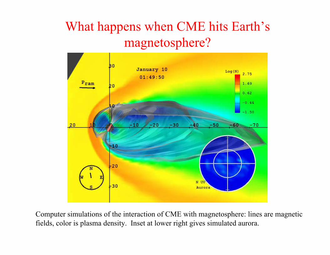
What happens when CME hits Earth’s magnetosphere?

Computer simulations of the interaction of CME with magnetosphere: lines are magnetic fields, color is plasma density. Inset at lower right gives simulated aurora.

Aurora as seen from space

Production of Auroral Light

• Auroral Spectrum consists of various emission lines: 557.7 nm (“Green line”), 1S → 1D

forbidden transition of atomic Oxygen (τ = 0.8 s)

630.0 nm (“Red line”), 1D→3P forbidden transition of Oxygen (τ = 110 s)

391.4 nm, 427.8 nm transitions in molecular Nitrogen ion N2

+ Hα (656.3 nm) and Hβ (486.1 nm) lines

due to proton precipitation

These lines are excited by electron and proton precipitation in 0.5-20 keV range. How do these particles get accelerated?

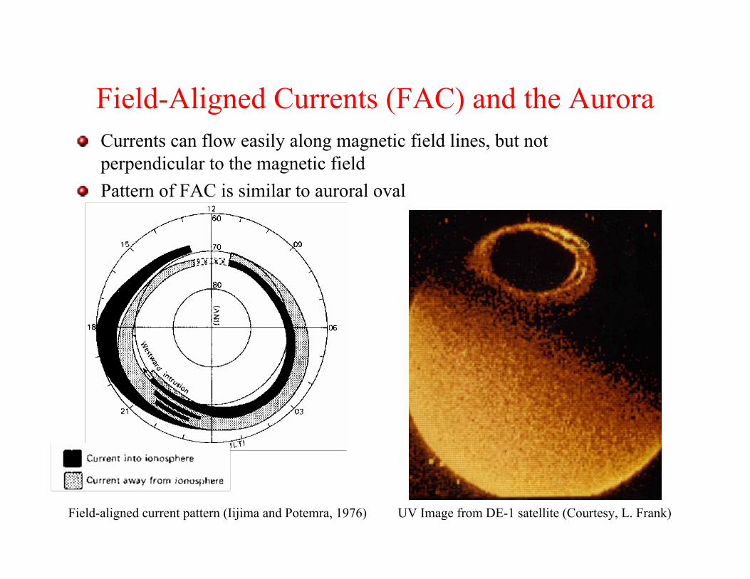
Field-Aligned Currents (FAC) and the AuroraCurrents can flow easily along magnetic field lines, but not perpendicular to the magnetic fieldPattern of FAC is similar to auroral oval

Field-aligned current pattern (Iijima and Potemra, 1976) UV Image from DE-1 satellite (Courtesy, L. Frank)

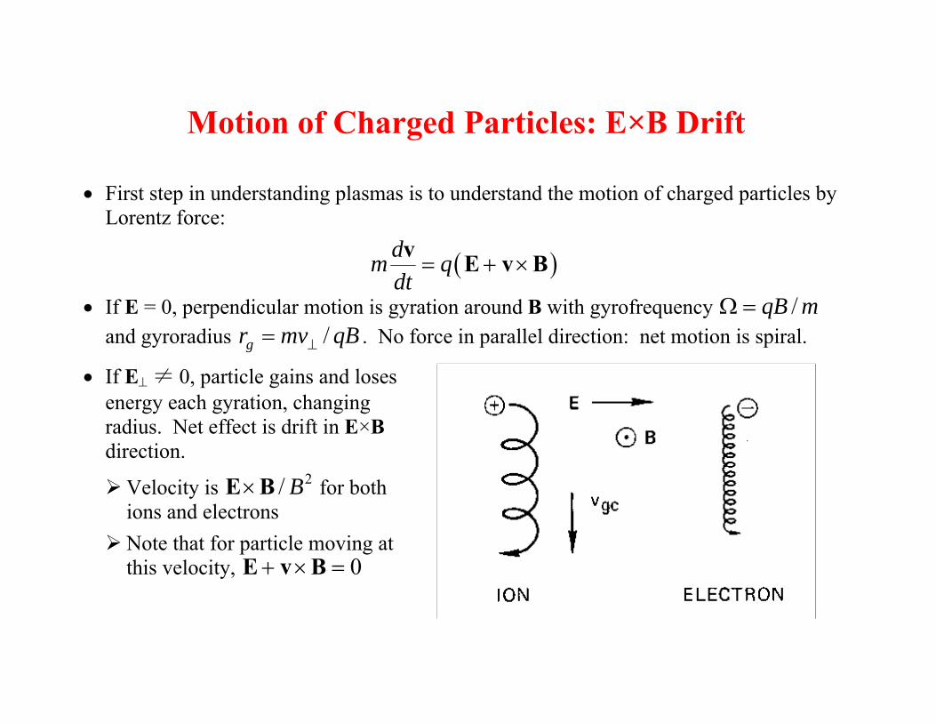
Motion of Charged Particles: E×B Drift • First step in understanding plasmas is to understand the motion of charged particles by

Lorentz force:

( )= + ×dm qdtv E v B

• If E = 0, perpendicular motion is gyration around B with gyrofrequency /Ω = qB m and gyroradius /⊥=gr mv qB . No force in parallel direction: net motion is spiral.

• If E⊥ ≠ 0, particle gains and loses energy each gyration, changing radius. Net effect is drift in E×B direction.

Velocity is 2/× BE B for both ions and electrons Note that for particle moving at this velocity, 0+ × =E v B

Motion of Charged Particles: Magnetic Mirroring

• Note that gyration of a charged particle comprises a current loop, which has a dipole moment, which is conserved during the particle’s motion:

2

2⊥μ =

mvB

• If particle moves into region of larger magnetic field, perpendicular velocity increases as well. However, total energy conservation then implies that parallel velocity must decrease. At some point, v|| → 0 and particle is reflected.

• In auroral zone, less than 1% of electrons from outer magnetosphere can precipitate into atmosphere (“diffuse aurora”). Strong auroral arcs require electric field parallel to the magnetic field.

Early evidence for E|| in Auroral Particles

“Monoenergetic Peak” in Electrons (Evans, 1974)

Proton and Electron Velocity Distributions from S3-3 satellite (Mozer et al., 1980)

Data from FAST satelliteFAST satellite is in polar orbit, apogee of 4000 km.

Overview of FAST passage through the auroral oval. Panels are (top to bottom): Magnetic field perturbation, electric field, electron energy, electron pitch angle, ion energy, and ion pitch angle.

Blue shading indicates downward current region, green is upward currents, and red is the Alfvenicacceleration region.

(Courtesy C. Carlson, from Auroral Plasma Physics, International Space Science Institute)

Electric Field Structures in the Auroral Zone

Perpendicular and parallel field observations indicate “U-shaped” or “S-shaped potential structures (R. Lysak, Ph.D. thesis, 1980)

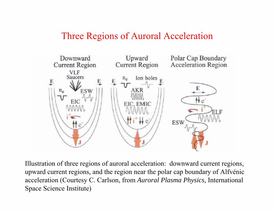
Three Regions of Auroral Acceleration

Illustration of three regions of auroral acceleration: downward current regions, upward current regions, and the region near the polar cap boundary of Alfvénic acceleration (Courtesy C. Carlson, from Auroral Plasma Physics, International Space Science Institute)

How to form and maintain parallel electric field?

Need to self-consistently maintain field with particle distributions:

0/∇ ⋅ = ρ εE• A simple such structure is the

plasma “double layer” • Note when particles are

reflected, their density increases. Thus, ion density is highest just to right of axis, and electron density to the left, making a “double layer” of charge.

• This is consistent with potential distribution

• Ions are accelerated to left, electrons to the right.

Detailed model of auroral potential structure(Ergun et al., 2000)

This model includes mirror force and 8 different particle populations.

Weak parallel electric field is found along flux tube, along with 2 strong double layers (called “Transition Layers” in the Figure).

Such models tell us that self-consistent parallel electric fields are possible, but how do they form and evolve?

In particular, where does the energy come from to support the particle acceleration?

Energy Supply for the Aurora

Downward motion of electrons and upward motion of ions gives field-aligned current.Therefore, magnetic field perturbations are also present.So auroral structure constitutes a transmission line.Energy can flow in as Poynting flux (S = E×B/μ0), and is dissipated in acceleration (j·E > 0).

Poynting’s Theorem:2 2

0

0 02 2⎛ ⎞ ⎛ ⎞ε∂ ×

+ + ∇ ⋅ = − ⋅⎜ ⎟ ⎜ ⎟∂ μ μ⎝ ⎠⎝ ⎠

E Bt

E B j E

Magnetohydrodynamics (MHD) • Evolution of plasmas can be most easily studied using MHD theory, which

describes average properties of the plasma, such as center-of-mass velocity u. Momentum equation becomes

ρ = × − ∇d pdtu j B

• Using Ampere’s Law (neglecting displacement current) we can write

2

0 0

12

⎛ ⎞ρ = ⋅∇ − ∇ +⎜ ⎟μ μ⎝ ⎠

d Bpdtu B B

• First term: Magnetic tension. Field lines “want” to be straight. Waves similar to waves on a string can be supported, called “Alfvén waves.” Alfvén waves propagate along magnetic field lines.

• Second term: Total pressure, including magnetic pressure term. Waves similar to sound waves are found, called “magnetosonic waves.” Magnetosonic waves can propagate in any direction.

Frozen-In Field Theorem • Currents in plasmas can be treated by Ohm’s Law, written in the rest frame of the

plasma ( )= σ + ×j E u B

• Magnetospheric plasma are essentially collision-free; thus, plasma has very high conductivity (except in ionosphere). As σ → ∞, Ohm’s Law becomes

0+ × =E u B

• Recall that this is condition for E×B drift! Put this into Faraday’s Law:

( )∂= −∇× = ∇× ×

∂tB E u B

• This equation leads to “Frozen-in Field Theorem”: Magnetic flux is carried along with the plasma. Can think of magnetic field lines “frozen in” plasma.

• Most MHD behavior can be treated qualitatively using these concepts: Magnetic tension Magnetic pressure Frozen-in magnetic fields

MHD Wave Modes

Linearized MHD equations give 3 wave modes:Slow mode (ion acoustic wave): • Plasma and magnetic pressure balance along magnetic field• Electron pressure coupled to ion inertia by electric field

Intermediate mode (Alfvén wave):• Magnetic tension balanced by ion inertia• Carries field-aligned current

Fast mode (magnetosonic wave):• Magnetic and plasma pressure balanced by ion inertia

• Transmits total pressure variations across magnetic field

( )/s sk c c pω = = γ ρ

( )0/A Ak V V Bω = = μ ρ

2 2 2 2A sk V k c⊥ω = +

(Note dispersion relations given are in low β limit)

Observations of Poynting flux from Polar Satellite (Wygant et al., 2000)

Left Panel: From Top to Bottom: Electric Field, Magnetic Field, Poynting Flux, Particle Energy Flux, Density

Right Panel: Particle Data. Top 3 panels are electrons, bottom 3 are ions. Panels give particles going down the field line, perpendicular to the field, and up the field line.

Alfvén Waves on Polar Map to Aurora and Accelerate Electrons

Left: Ultra-violet image of aurora taken from Polar satellite. Cross indicates footpoint of field line of Polar (Wygant et al., 2000)

Right: Electron distribution function measured on Polar. Horizontal direction is direction of magnetic field. Scale is ±40,000 km/s is both directions (Wygant et al., 2002)

How are Alfvén waves/field-aligned currents produced?

Linear mode conversion: Mode conversion can take place from a surface Alfvén wave (Hasegawa, 1976), from compressional plasma sheet waveguide modes (Allan and Wright, 1998), or from compressional waves in plasma sheet (Lee et al., 2001).

Bursty Bulk Flows: Localized flow regions can generate Alfvén waves due to the twisting and compression of magnetic field lines (Song and Lysak, 2000), perhaps associated with localized reconnection. BBF association with Alfvénic Poynting flux observed by Geotail (Angelopoulos et al., 2002).

Reconnection with two-fluid effects: Two-fluid (Hall) effects lead to a By signature and the generation of field-aligned currents. Bursty reconnection at this point will launch Alfvén waves.

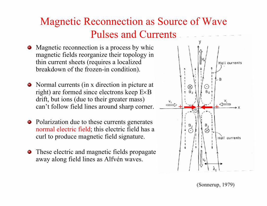
Magnetic reconnection is a process by which magnetic fields reorganize their topology in thin current sheets (requires a localized breakdown of the frozen-in condition).

Normal currents (in x direction in picture at right) are formed since electrons keep E×B drift, but ions (due to their greater mass) can’t follow field lines around sharp corner.

Polarization due to these currents generates normal electric field; this electric field has a curl to produce magnetic field signature.

These electric and magnetic fields propagate away along field lines as Alfvén waves.

(Sonnerup, 1979)

λi

+ +−

Magnetic Reconnection as Source of Wave Pulses and Currents

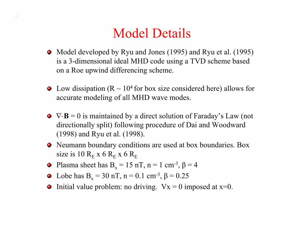
Model DetailsModel developed by Ryu and Jones (1995) and Ryu et al. (1995) is a 3-dimensional ideal MHD code using a TVD scheme based on a Roe upwind differencing scheme.

Low dissipation (R ~ 104 for box size considered here) allows for accurate modeling of all MHD wave modes.

∇⋅B = 0 is maintained by a direct solution of Faraday’s Law (not directionally split) following procedure of Dai and Woodward (1998) and Ryu et al. (1998).Neumann boundary conditions are used at box boundaries. Box size is 10 RE x 6 RE x 6 RE

Plasma sheet has Bx = 15 nT, n = 1 cm-3, β = 4Lobe has Bx = 30 nT, n = 0.1 cm-3, β = 0.25Initial value problem: no driving. Vx = 0 imposed at x=0.

Wave Speed Profilest= 0.00, x= 2.00, y= 0.00, va, cf, cs

-3 -2 -1 0 1 2Z

0

500

1000

1500

2000

2500

va, c

f, c

s (k

m/s

)

Alfvén speed

Magnetosonic speed

Sound speed

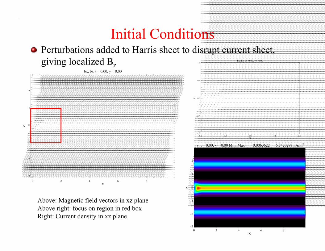
Initial ConditionsPerturbations added to Harris sheet to disrupt current sheet, giving localized Bz

bx, bz, t= 0.00, y= 0.00

0 2 4 6 8X

-3

-2

-1

0

1

2

Z

bx, bz, t= 0.00, y= 0.00

0.0 0.5 1.0 1.5 2.0X

-1.0

-0.5

0.0

0.5

1.0

Z

jy. t= 0.00, y= 0.00 Min, Max= 0.0063622 6.7420297 nA/m2

0 2 4 6 8X

-3

-2

-1

0

1

2

Z

Above: Magnetic field vectors in xz planeAbove right: focus on region in red boxRight: Current density in xz plane

Evolution of localized reconnection runV on z=0 plane Total pressure on y=0 plane

Jx on y=1.5 plane Jx on z=1.8 plane (boundary layer)

The “Auroral Transmission Line” • The propagation of Alfvén waves along auroral field lines may be

considered to be an electromagnetic transmission line. Energy is propagated in the “TEM” mode, the shear Alfvén wave at the Alfvén speed, 0/= μ ρAV B

• Transmission line is filled with a dielectric medium, the plasma, with an inhomogeneous dielectric constant 2 21 / ( )ε = + Ac V z

• Can define a characteristic admittance for the transmission line

01/Σ = μA AV

• Transmission line is “terminated” by the conducting ionosphere. In general, Alfvén waves will reflect from this ionosphere, or from strong gradients in the Alfvén speed.

Ionospheric Currents • Field-aligned currents must close in the ionosphere.

• Collisions with neutral atoms in the ionosphere can disrupt E×B motions of particles, especially for ions.

• For /in i iqB mν ≈ Ω ≡ , ions move in direction of electric field, giving Pedersen current.

• For in iν >> Ω and e eν << Ω , ions are tied to neutrals while electrons can E×B drift, giving Hall current.

• These currents flow in a thin layer (between 100 and 500 km altitude), so we can integrate over height:

P P H Hdz dzΣ = σ Σ = σ∫ ∫

B

E jP

ion

B

E elec

jH

Reflection of Alfvén Waves by the Ionosphere

Ionosphere acts as terminator for Alfvén transmission line.

But, impedances don’t match: wave is reflected

Usually ΣP >> ΣA, so electric field of reflected wave is reversed (“short-circuit”)

A complication: Electrons hitting ionosphere increase plasma density and thus, conductivity.

(Mallinckrodt and Carlson, 1978)

Resonances of Alfvén Waves

Alfvén can bounce from one ionosphere to the other: Field Line Resonance (periods 100-1000 s)

However, Alfvén speed has sharp gradient above ionosphere: wave can bounce between ionosphere and peak in speed: Ionospheric Alfvén Resonator (Periods 1-10 s)

Fluctuations in the aurora are seen in both period ranges. Feedback can structure ionosphere at these frequencies.

Profiles of Alfvén speed for high density case (solid line) and low-density case (dashed line). Ionosphere is at r/RE = 1. Sharp rise in speed can trap waves (like quantum mechanical well). Note speed can approach c in low-density case.

Simulations of Alfvén Wave Pulse along auroral field line

ExBy

r

Pea

k of

Alfv

en

spee

d

Ionosphere

Auroral movie (courtesy J. Semeter, Boston U.) Real time imaging; field of view approx. 20 km x 20 km

Alfvén wave dynamics likely responsible for this structure!

Auroral Density Cavity

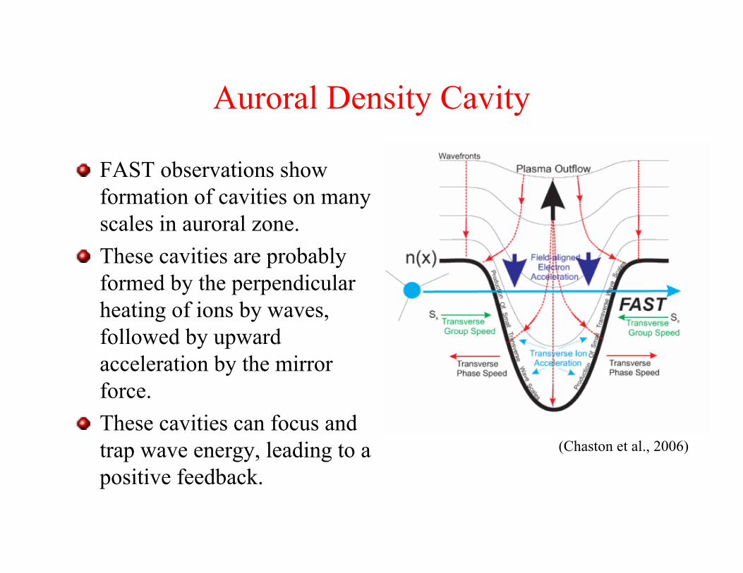
FAST observations show formation of cavities on many scales in auroral zone.These cavities are probably formed by the perpendicular heating of ions by waves, followed by upward acceleration by the mirror force.These cavities can focus and trap wave energy, leading to a positive feedback.

(Chaston et al., 2006)

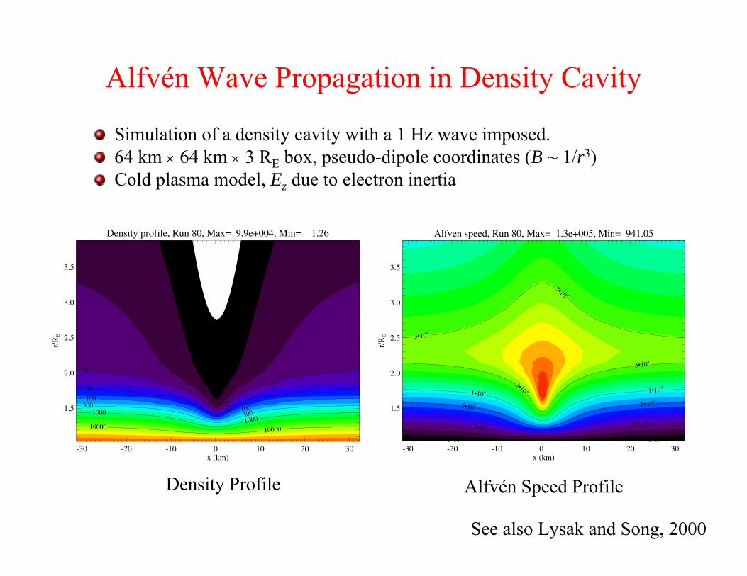
Alfvén Wave Propagation in Density Cavity

Simulation of a density cavity with a 1 Hz wave imposed.64 km × 64 km × 3 RE box, pseudo-dipole coordinates (B ~ 1/r3) Cold plasma model, Ez due to electron inertia

See also Lysak and Song, 2000

Density profile, Run 80, Max= 9.9e+004, Min= 1.26

-30 -20 -10 0 10 20 30x (km)

1.5

2.0

2.5

3.0

3.5

r/R

E

3

3

3

10

10

30

30

100

100300

30010001000

10000 10000

Alfven speed, Run 80, Max= 1.3e+005, Min= 941.05

-30 -20 -10 0 10 20 30x (km)

1.5

2.0

2.5

3.0

3.5

r/R

E

1•1031•103

2•1032•103

5•1035•103

1•104

1•104

3•104

3•10 4

3•104

3•10 4

Density Profile Alfvén Speed Profile

Evolution of Run: Ex, By at y=0

• Note structuring of Ex on density gradient due to phase mixing. By not as structured since short scale waves become electrostatic.

• Evident phase progression away from center line.• Note ΣP = 3 mho, ΣH = 0 for this run.

Structure Perpendicular to Field: Ex

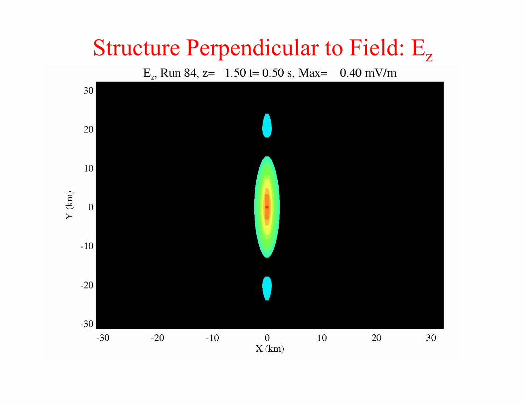
Structure Perpendicular to Field: Ez

Structure Perpendicular to Field: Poynting flux

Note Poynting flux perpendicular to field is toward center of structure (green/red: toward positive x; black/blue: toward negative x), opposite to phase motion, consistent with dispersion relation and observations.

Effects of Changing ConductanceEx, Run 81, y= -0.25 t=10.00 s, Max= 7362.89 mV/m

-30 -20 -10 0 10 20 30X (km)

1.5

2.0

2.5

3.0

3.5

r/R

E

Ex, Run 84, y= -0.25 t=10.00 s, Max= 8482.34 mV/m

-30 -20 -10 0 10 20 30X (km)

1.5

2.0

2.5

3.0

3.5

r/R

E

ΣP = 1 mho ΣP = 3 mho ΣP = 10 mho

Structuring of electric field by phase mixing closely connected with ionospheric conductance: higher conductance allows finer-scale structuring.

Hall effects: Run with ΣP = 1 mho; ΣH = 2 mho

Finite Hall conductance leads to a twisting of electric field pattern, even for low conductance case.

Ez Structure with Hall conductance

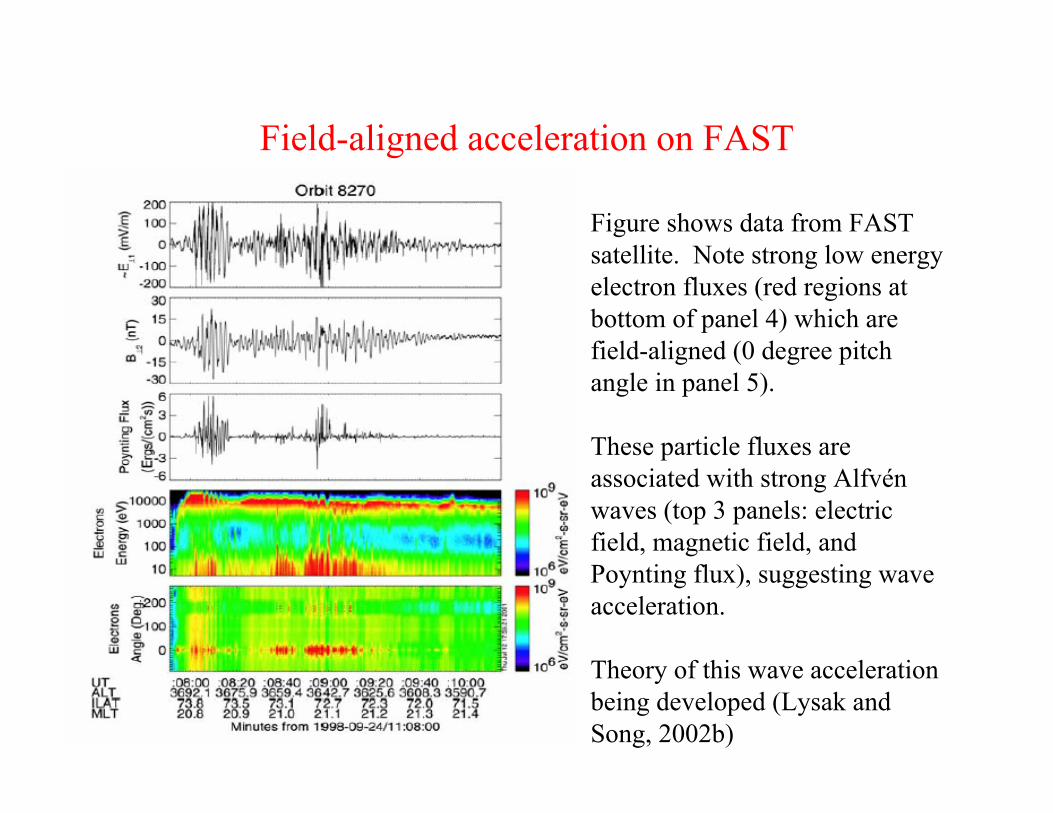
Field-aligned acceleration on FAST

Figure shows data from FAST satellite. Note strong low energy electron fluxes (red regions at bottom of panel 4) which are field-aligned (0 degree pitch angle in panel 5).

These particle fluxes are associated with strong Alfvén waves (top 3 panels: electric field, magnetic field, and Poynting flux), suggesting wave acceleration.

Theory of this wave acceleration being developed (Lysak and Song, 2002b)

Some outstanding problems in space plasma physics being studied at UM

Formation of parallel electric fields and their connection to the energy supplyStructuring of auroral arcs: some arcs are as narrow as 100 m, others are 5-10 km. How to understand all these scales?Generation of field-aligned currents and Alfvén waves. New measurements from Cluster (4 satellites) show large wave energy flows in geomagnetic tail.Development of magnetic reconnection: magnetic fields can annihilate, releasing large amounts of energy. How does this happen and how is it related to auroral particle acceleration and the overall dynamics of the magnetosphere?

So what do our grad students do?Build flight hardware. Our group specializes in building electric field instruments together with on-board processors to take data from satellite and rocket missions.

Develop software to analyze data. Satellite missions involve large amounts of raw data, and sophisticated codes are needed to organize this data into usable form so that it can be interpreted.

Develop theoretical models to understand data. New data, especially multipoint data from Cluster, requires refinement of earlier, simpler ideas.

Develop numerical simulation models. We specialize in large-scale supercomputer codes to model wave interactions with the ionosphere and within the magnetosphere.