space requirements determination of the production rate determination of batch production quantities...
TRANSCRIPT

Space Requirements
• Determination of the Production Rate
• Determination of Batch Production Quantities– Economic Order Quantity Models
– Reject Allowance Problem
• Determination of Equipment Requirements
• Determination of Employee Requirements– Manual Assembly Operators
– Machine Operators
• Determination of Space Requirements
• Tables for Aisle Allowance, Food Services and Restrooms
• Other Methods to Determine Space Requirements
• Parking Space

Determination of the Production Rate
• The production rate of a department is a major determinant of the amount of space required. The production rate of a processing station is the number of units produced per time unit. The production rate can be determined from a marketing forecast of the finished product.
• Notation: a = arrival rate of raw material.
d = demand rate of a product.
p = production rate of a processing station.
s = scrap probability of an inspection station.
r = rework probability of an inspection station.
1
1
p
s
d
a
r

Example 1
Consider the operation process chart shown in the Figure. The percentage of rejected parts at inspection stations 1, 2 and 3 are 5%, 4% and 6%, respectively. The annual operating time is 2,500 hours, and the annual demand forecast for the product is 490,000 units. Due to possible forecasting errors, 10,000 additional units per year are required. Find the production rate at each station.
1
2
1
3
4
2
5
6
3
p1 p3
p2 p4
s2
p5
p6
d
s3
s1
(1)(2)

Example 1 Solution
d units hr
490 000 10 000
2 500200
, ,
,/ .
p pd
sunits hr5 6
31
200
0 94212 76
( ) .. / .
p pp
sunits hr3 4
5
21
212 76
0 9622163
( )
.
.. / .
p pp
sunits hr1 2
5
1
2
1
2 212 76
0 95447 92
( )
.
.. / .
(good units)
1
2
1
3
4
2
5
6
3
p1 p3
p2 p4
s2
p5
p6
d
s3
s1
(1)(2)

Example 2
Consider a product that requires a single operation. After the operation is performed, each unit is inspected. A unit passes inspection with probability 0.92, is scrapped with probability 0.05, or has to be reworked with probability 0.03. If the demand for this product is 82,000 units per year and the annual operating time is 2,500 hours, determine the production rate at the processing station.
1
1
p
s
d
a
r
d units hr 82 000
2 50032 80
,
,. / .
pd
s runits hr
( )
.
.. / .
1
32 80
0 923565
a p r units hr ( ) . . . / .1 3565 0 97 34 58
(good units)
Determination of Batch Production Quantities
• In process layout, a given machine can be used to process different products. In certain product layouts, the same production (or assembly) line can be used to produce (or assemble) similar products with the same process plan. In both of these cases, jobs are produced in batches. Optimal batch production quantities can be computed using an inventory control model.
• Process layouts are also used in job shops where “one-shot” jobs are received and processed. Rather than producing for inventory, the order is processed and shipped to the customer. The reject allowance problem determines the optimal production lot size for a given order when a portion of the lot may be defective.
Economic Order Quantity (EOQ) Model
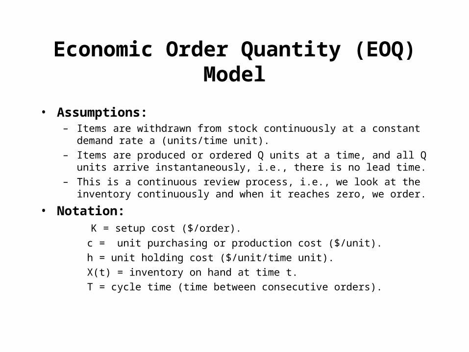
• Assumptions:– Items are withdrawn from stock continuously at a constant demand rate a
(units/time unit).
– Items are produced or ordered Q units at a time, and all Q units arrive instantaneously, i.e., there is no lead time.
– This is a continuous review process, i.e., we look at the inventory continuously and when it reaches zero, we order.
• Notation: K = setup cost ($/order).
c = unit purchasing or production cost ($/unit).
h = unit holding cost ($/unit/time unit).
X(t) = inventory on hand at time t.
T = cycle time (time between consecutive orders).

Economic Order Quantity (EOQ) Model (cont.)
• Total cost per cycle (TCC) = ordering cost + holding cost:
TCC K cQ hQ Q
aK cQ
hQ
a
2 2
2
• Total cost per unit time (TC) = TCC
T
TC
K cQhQ
aQ
a
a K
Qa c
hQ
2
2
2
X(t)
Q
T
-a
t

Economic Order Quantity (EOQ) Model (cont.)
• Minimization of TC with respect to Q:
• Solution:
d TC
d Q
a K
Q
h
2 2
0
Qa K
h*
2
TQ
a
a K
ha
K
a h*
*
22
TCa K
Qa c
hQKa h a c*
*
*
22
aKQ
hQ2
ca
Q*
TC
Q
TC*
: EOQ Formula

EOQ Model with Quantity Discounts
• Consider the EOQ model with the following unit cost structure with discount for larger amounts:
For 0 Q < M1 the unit cost is c0
M1 Q < M2 c1
…. ….
Mn-1 Q < Mn cn-1
Mn Q cn
• Mi, i = 1,…, n, represent the price break points, such that
M1 < M2 < …. < Mn.
• Assumption: unit costs are such that c0 > c1 > …. > cn.

EOQ Model with Quantity Discounts (cont.)
Algorithm to find Q*:
Step 1: Determine QKa
h
2.
Step 2: Find the interval (Mi, Mi+1), where Q falls in.
Step 3: Compare the total cost for the amount Q,
with the total cost for the amounts Mi+1, Mi+2, …, Mn,
TC a K h c ai 2 ,
TC Ma K
M
h Ma cj
j
jj( ) .
2
Step 4: Select the amount corresponding to the minimum total cost per time unit: TC* = min {TC, TC(Mi+1), TC(Mi+2), …, TC(Mn)}.

Example 3: EOQ Model
The publisher of a newspaper periodically replenishes paper for stock. Paper comes in large rolls. The demand is 32 rolls/ week. The cost of ordering is $25 and the cost per roll is $40. The cost of keeping paper is $1/roll/week. Determine the EOQ and the optimal cycle time.
a = 32 rolls/week,
K = $25/order,
h = $1/roll/week.
TQ
aweeks*
*.
40
32125
Qa K
hrolls*
2 2 32 25
140

Example 4: EOQ Model with Quantity Discounts
In the newspaper example, find Q* given the following quantity discounts:
1 - 9 rolls: $12/roll,
10 - 49 rolls: $10/roll,
50 - 99 rolls: $9.50/roll,
100 rolls or more:$9/roll.
Q rolls
2 35 25
140 TC week( ) $360 /40 2 32 25 1 10 32
TC week( ) . $345 /5032 25
50
1 50
29 5 32
TC week( ) $346 /100
32 25
100
1 100
29 32
40 (10, 49)
Min {$360, $345, $346}=$345 Q* = 50 rolls

Reject Allowance Problem
In job shops, one time jobs are received and processed. There is no production to inventory. Each batch is only produced once. If there is a defective rate, how many units must be produced? The following expected profit model is formulated to determine the optimal batch size:
max [ ( )] { ( , ) ( , )} ( )Qx
Q
QE P Q R Q x C Q x p x 0
where Q = lot size,
x = number of good parts,
pQ(x) = P{X=x : lot size is Q}, x=0,1,…,Q,
R(Q,x) = revenue for producing Q parts with exactly x good ones,
C(Q,x) = cost for producing Q parts with exactly x good ones,
P(Q,x) = R(Q,x) - C(Q,x) : profit for producing Q parts with x good ones,
E[] = expected value.

Example 5
• A company receives an order for 10 machined parts. The unit sale price is $1,000. Only one production can be made due to the long setup time required and short due date of the order. If 8 or fewer parts are acceptable, the customer will cancel the order. If 9 or 10 parts are acceptable, the customer will purchase all of them. If more than 10 parts are acceptable, the customer will only buy 10. The remaining parts, good or bad, can be sold for $25 each. The cost of producing a part is estimated to be $600. Find the optimal lot size.
• Probability mass function pQ(x):
Number of good partsLot size 7 8 9 10 11 12 13 14
10 0.2 0.3 0.3 0.211 0.2 0.3 0.3 0.212 0.1 0.2 0.3 0.2 0.213 0.2 0.2 0.3 0.2 0.114 0.2 0.2 0.3 0.2 0.1

Example 5 Solution
R Q x
Q
x Q x
Q
x
x
x Q
( , ) ( )
( )
,...,
,
,...,
25
1000 25
1000 10 25 10
0 8
9 10
11
C(Q,x) = C(Q) = 600Q
E P Q R Q x C Q x p x R Q x p x C QQ Qx
Q
x
Q[ ( )] { ( , ) ( , )} ( ) [ ( , ) ( )] ( )
00
E P Q Q p x x Q x p x Q p x Q
x p x p x Q
xQ Q
x
Q
xQ
Q Qx
Q
x
[ ( )] ( ) [ ( )] ( ) ( ( )] ( )
( ) ( )
25 1000 25 10000 25 10 600
975 9750 575
0
8
119
10
119
10

Example 5 Solution (cont.)
• E[P(10)] = 975(90.3+100.2) + 97500 - 57510 = -1167.50
• E[P(11)] = 975(90.3+100.3) + 97500.2 - 57511 = 1182.50
• E[P(12)] = 975(90.2+100.3) + 9750(0.2+0.2) - 57512 = 1680.00
• E[P(13)] = 975(90.2+100.2) + 9750(0.3+0.2+0.1) - 57513 = 2080.00
• E[P(14)] = 975(100.2) + 9750(0.2+0.3+0.2+0.1) - 57514 = 1700.00
Optimal lot size: Q* = 13 units
Expected profit: E[P(Q*)] = $2,080.00

Determination of Equipment Requirements
Given the desired production rate at each processing stage, we can determine the number of required machines:
where Pij = production rate for product i on machine j (units/period),
Tij = processing time for product i on machine j (hrs./unit),
Hij = time units available per period for the processing of product i on
machine j (hrs.),
Mj = number of machines of type j required,
n = number of products.
MP T
Hjij ij
iji
n
1

Example 5
CIN-A1 Workcenters are used to produce three types of parts, {1, 2, 3}. Production rates and unit processing times for the different items are given in the following table:
The facility operates one shift per day (8 hrs./day = 480 min./day). Determine the number of workcenters required to meet production requirements.
Hi = min. available to process item i per day (Hi = 480 min.),
MA = number of workcenters.
Item typei
Production ratePi (units/day)
Unit processing timeTi (min./unit)
1 100 62 200 93 50 12
MP T
Hworkcenters CIN AA
i i
ii
1
3 100 6 200 9 50 12
4806 25 7 1. .

Employee Requirements - Manual Assembly
In the case of manual assembly operations, the number of employees required is determined in the same way machine requirements are calculated:
where Pij = production rate for assembly operation j of product i (units/period),
Tij = standard time for assembly operation j of product i (hrs./unit),
Hij = time units available per period for assembly operation j of product i
(hrs.),
Aj = number of operators required for assembly operation j,
n = number of products.
AP T
Hjij ij
iji
n
1

0
2
4
6
8
10
12
14
16
18
20
O-1 M-1
L-1
U-1
L-1
I
I
L
R
U
L
R
O-1 M-1 M-2
I&T
I&T
I&T
L
R
U
L
R
L-1
U-1
L-1
U-2
L-2
U-2
R
R
U
L
U
L-1
I&T
U-2
L-2
I&T
I&T
U-3
L-3
I&T
U-1
L-1
I&T
U-2
L
R
L
U
R
U
L
R
R
U
U
L
R
R
O-1 M-1 M-2 M-3
LEGEND:
O : OperatorM : MachineL : LoadU : UnloadI : InspectionT : TravelR : Automatic run
: Idle time
Multiple Activity Chart Analysis of Multi-Machine Assignment

Employee Requirements - Machine Operators
• The number of machine operators required depends on the number of machines tended by one or more operators. The determination of the number of machines to be assigned to one operator can take two approaches:
deterministic, probabilistic.
• A deterministic approach is to employ the multiple activity chart. This chart shows the multiple activity relationships graphically against a time scale. The chart is useful in analyzing multiple activity relationships, specially, when non-identical machines are supervised by a single operator.
• Let a = concurrent activity time (loading, unloading, etc.),
b = independent operator activity time (inspecting, packing, etc.),
t = independent machine activity time (automatic run),
n’ = maximum number of machines that can be assigned to an operator.

Employee Req. - Machine Operators (cont.)
• Note that n’ may be non-integer.
• Let m = (integer) number of machines assigned to an operator,
Tc = repeating cycle time,
I0 = idle operator time during a repeating cycle,
Im = idle time per machine during a repeating cycle.
na t
a b'
Ta t
m a b
m n
m nc
( )
'
'
Ia t m a b m n
m n0 0
( ) ( ) '
'
(1)

Employee Req. - Machine Operators (cont.)
• Substituting (1) into (2),
Im a b a t m n
m nm
( ) ( ) '
'0
TC m c m cT
mc( ) ( ) 1 2 (2)
TC mc m c a t
mc m c a b
m n
m n( )
( )( )
( )( )
'
'
1 2
1 2
• Let c1 = cost per operator - hr.,
c2 = cost per machine - hr.,
TC(m) = cost per unit produced, based on the assignment of m machines per operator.

Employee Req. - Machine Operators (cont.)
• We want to find the value of m that minimizes TC(m).
• Note that for m n’, m () TC(m) (),and for m > n’, m () TC(m) ().
• If n’ is integer, n’ is the optimal number of machines per operator.
Otherwise, let n < n’ < n+1. In this case, TC(n) and TC(n+1) have to be compared:
TC n
TC n
c n c a t
c n c n a b
n
n
n
n
( )
( )
( )( )
[ ( ) ] ( )
'
1 1 11 2
1 2
where cc
12
.
• If <1, assign n machines per operator.
If >1, assign n+1 machines per operator.

Example 6
• Semiautomatic machines are used to produce a particular product. It takes 4 minutes to load and 3 minutes to unload a machine. A machine runs automatically for 25 minutes in producing one unit of the product. Travel time between machines is 20 seconds. While machines are automatically running, the operator inspects the unit previously produced; 75 seconds are required to inspect one unit. An operator costs $15 per hour, and a machine costs $40 per hour.
a) Determine the number of machines assigned to an operator to minimize the cost per unit produced.
a = 4 + 3 = 7 min., b = 20 + 75 = 95 sec. = 1.58 min., t = 25 min.,
c1 = $15/hr. = $0.25/min., c2 = $40/hr. = $0.67/min.
n'.
.
7 25
7 158373
m* = 3 machines/operator.TC( )
( . . )( )$24.3
0 25 3 0 67 7 25
30
TC( ) ( . . )( . ) $25.4 0 25 4 0 67 7 158 03

Example 6 (cont.)
b) For what range of values of machine cost per hour will the optimal assignment determined in part (a) be economic.
TC(3) TC(4),
( . )( )( . )( . ),
0 25 3 7 25
30 25 4 7 1582
2
c
c
(0.25 + 3c2) 1.24 (0.25 + 4c2),
0.0607 0.27c2 c2 0.225,
c2 $0.225/min. = $13.48/hr.

Space Req’s.: Workstation Specification
• A workstation consists of the fixed assets needed to perform a specific operation(s).
• The equipment space consists of space for - The equipment - Machine maintenance
- Machine travel - Plant services
• Equipment space requirements are available from machinery data sheets (provided by the supplier). If this data is not available, the following information must be obtained for each machine:
- Machine manufacturer and type - Maximum travel to the left
- Machine model and serial number - Maximum travel to the right
- Location of machine safety stops - Static depth at maximum point
- Floor loading requirement - Maximum travel towards the operator
- Static height at maximum point - Maximum travel away from the operator
- Maximum vertical travel - Maintenance requirements and areas
- Static width at maximum point - Plant service requirements and areas

Space Req’s.: Workstation Specification (cont.)
• Area requirements for a machine: Total width = (static width) + (max. travel to left) + (max. travel to right)
Total depth = (static depth) + (max. travel toward operator) + (max. travel away from operator)
Area (machine + machine travel) = (total width) * (total depth)
• The materials areas consists of space for– Receiving and storing materials
– In-process materials
– Storing and shipping materials
– Storing and shipping waste and scrap
– Tools, fixtures, jigs, dies, and maintenance materials
• The personnel areas consists of space for– The operator
– Material handling
– Operator ingress and egress

General Guidelines for Design of Workstations
• The operator should be able to pick up and discharge materials without walking or making long or awkward reaches.
• The operator should be utilized efficiently and effectively.
• The time spent manually handling materials should be minimized.
• The safety, comfort and productivity of the operator must be maximized.
• Hazards, fatigue and eye strain must be minimized.
• A workstation sketch is required to determine total area requirements.

Space Req’s.: Department Specification
• Department area requirements are not simply the sum of the areas of the individual workstations included in each department.
• Machine maintenance, plant services, incoming and outgoing materials, and operator ingress and egress areas for various workstations must be combined.
• Additional space is required for material handling within the department. Space requirements for aisles can be approximated since the relative sizes of the loads to be handled are known.

Tables for Aisle Allowance
If the Largest Load isAisle Allowance
(Percentage of NetArea Required)
Less than 6 ft2
Between 6 and 12 ft2
Between 12 and 18 ft2
Greater than 18 ft2
5 – 1010 – 2020 – 3030 - 40
Type of Flow Aisle Width(ft)
Tractors3-ton Forklift2-ton Forklift1-ton Forklift
Narrow Aisle TruckManual Platform Truck
PersonnelPersonnel with Doors Openinginto the Aisle from One Side
Personnel with Doors Openinginto the Aisle from Two Sides
12111096536
8
Table 1. Aisle Allowance EstimatesTable 2. Recommended Aisle Widths
for Various Types of Flow
In Example 7,
108 6
12 6(20 10) 13.33 %.

Example 7
A planning department for the ABC Company consists of 13 machines that perform turning operations. Five turret lathes, six automatic screw machines, and two chuckers are included in the planning department. Bar stock, in 8-ft bundles, is delivered to the machines. The footprints for the machines are 412 ft2 for the turret lathes, 414 ft2 for the screw machines, and 56 ft2 for the chuckers. Personnel space footprints of 45 ft2 are used. Materials storage requirements are estimatefd to be 20 ft2 per turret lathe, 40 ft2 per screw machine, and 50 ft2 per chucker. An aisle space allowance of 13% is used. The space calculations are summarized in the table below.
Service Requirements Area (ft2)Workstation Quantity
Power CompressedAir
OtherFloor
LoadingCeilingHeight Equipment Material Personnel Total
TurretLathe
5 440 VAC
10 CFM @100 psi
150 PSF 4’ 240 100 100 440
ScrewMachine
6 440 VAC
10 CFM @100 psi
190 PSF 4’ 336 240 120 696
Chucker 2 440 VAC
10 CFM @100 psi
150 PSF 5’ 60 100 40 200
Net Area Required13% Aisle AllowanceTotal Area Required
13361741510

Food Services
Beginning ofLunch Break
Time Sat DownIn Chair
End ofLunch Break
11:30 am11:50 am12:10 pm12:30 pm
11:40 am12:00 noon12:20 pm12:40 pm
12:00 noon12:20 pm12:40 pm1:00 pm
Classification Allowance perPerson (ft.2)
CommercialIndustrialBanquet
16 – 1812 – 1510 – 11
Table 3. Shift Timing for 30 min.Lunch Breaks
Table 4. Space Requirementsfor Cafeterias
Number ofMeals Served
AreaRequirements
(ft.2)100 – 200200 – 400400 – 800
800 – 13001300 – 20002000 – 30003000 - 5000
500 – 1000800 – 1600
1400 – 28002400 – 39003250 – 50004000 – 60005500 – 9250
Table 5. Space Requirementsfor Full Kitchens

Example 8
• Statement:
If a facility employs 600 people and they are to eat in three equal 30 min. shifts, how much space should be planned for the cafeteria with vending machines, serving lines, or a full kitchen?
• Solution:– If 36-in. square tables are to be utilized, Table 4 indicates 12 ft.2 are required for
each of the 200 employees to eat per shift. Therefore, a 2,400 ft.2 cafeteria should be planned. If a vending area is to be used in conjunction with the cafeteria, an area of 200 ft.2 should be allocated for vending machines. Thus, a vending machine food service facility would require 2,600 ft.2
– A service line may serve 70 employees in the first third of the meal shift. Therefore, three serving lines of 300 ft.2 each should be planned. A total of 3,300 ft.2 would be required for a food service facility using serving lines.
– A full kitchen will require 3,300 ft.2 for serving lines plus (from Table 5) 2,100 ft.2 for the kitchen. Therefore, a total of 5,400 ft.2 would be required for a full kitchen food service facility.

Restrooms
Maximum Number ofEmployees Presentat any One Time
Minimum Numberof Toilets Needed
1 – 1516 – 3536 – 5556 – 80
81 – 110111 – 150Over 150
123456
1 additional toiletfor each additional
40 employees
Type ofEmployment
Number ofEmployees
Minimum NumberOf Sinks
Non-industrial(Office and
Public Facilities)
1 – 1516 – 3536 – 6061 – 9091 – 125Over 125
12345
1 sink for eachadditional 45employees
Industrial(Manufacturingand warehouse
Facilities)
1 – 100
Over 100
1 sink for each10 employees
1 sink for eachadditional 15employees
Table 6. Number of Toilets Neededfor Number of Employees
Table 7. Number of Sinks Needed for Typeof Employment and Number of Employees

Other Methods to Determine Space Requirements
• Converting Method
– The present space requirements are converted to those required for the proposed layout. It is important to establish valid assumptions, because the total space required is not a linear function of the production quantity.
– This method is used to determine space requirements for supporting service, storage areas, etc.
• Roughed-out Layout Method
– Templates or models are placed on the layout to estimate the general configuration and space requirements.

Other Methods to Determine Space Req’s. (cont.)
• Space-Standards Method
– In certain cases industry standards can be used to determine space requirements.
– Standards may be established based on past successful applications.
• Ratio Trend and Projection Method
– One can establish a ratio of square feet to some other factor that can be measured and predicted for the proposed layout. For example,
square feet per machine
square feet per operator
square feet per unit produced
square feet per labor-hour

Parking Space
( angular one-way )
( 900 two-way )
( cross aisle )( cross aisle )
Parking Space (cont.)
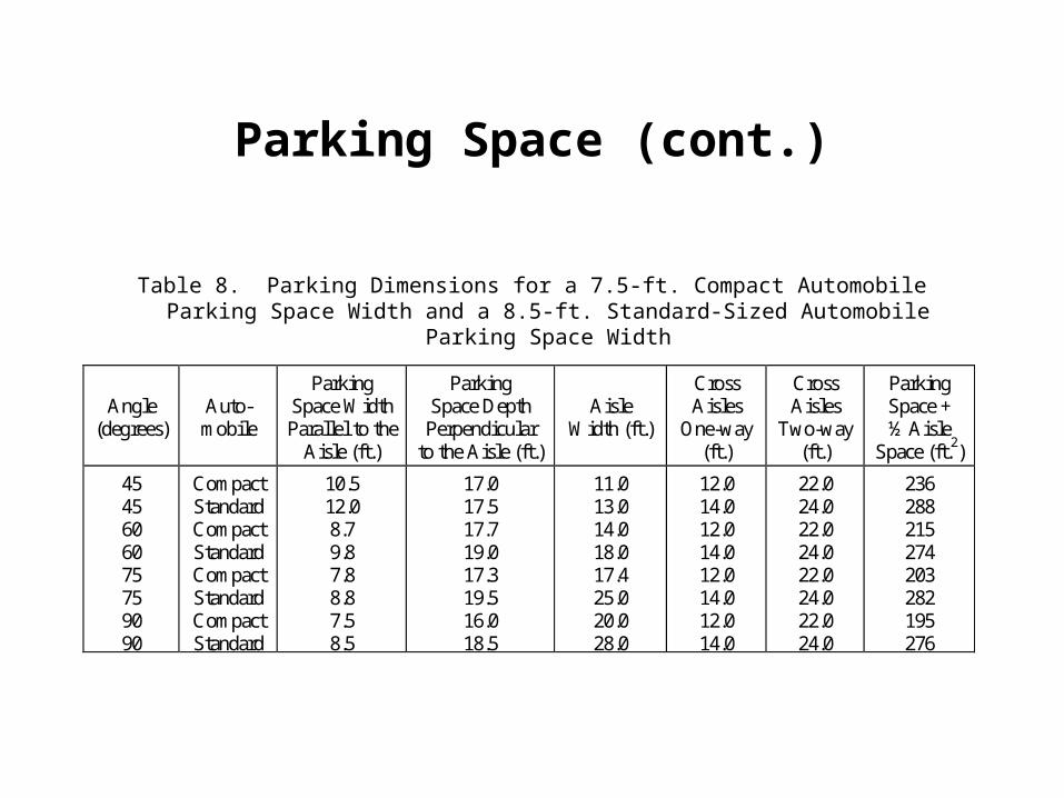
Table 8. Parking Dimensions for a 7.5-ft. Compact Automobile Parking Space Width and a 8.5-ft. Standard-Sized Automobile Parking Space Width
Angle(degrees)
Auto-mobile
ParkingSpace WidthParallel to the
Aisle (ft.)
ParkingSpace DepthPerpendicular
to the Aisle (ft.)
AisleWidth (ft.)
CrossAisles
One-way(ft.)
CrossAisles
Two-way(ft.)
ParkingSpace +½ Aisle
Space (ft.2)
4545606075759090
CompactStandardCompactStandardCompactStandardCompactStandard
10.512.08.79.87.88.87.58.5
17.017.517.719.017.319.516.018.5
11.013.014.018.017.425.020.028.0
12.014.012.014.012.014.012.014.0
22.024.022.024.022.024.022.024.0
236288215274203282195276

Parking Space (cont.)
Parking space + 1/2 aisle space (for 600 standard)
= 19.0 9.8 + 18.0 9.8 / 2 = 186.2 + 88.2 274 ft.2
Parking space Parking space
Depth perpendicular to aisle (19.0 ft.) Aisle width (18.0 ft.)
Wid
th p
aral
lel t
o
aisl
e (9
.8 f
t.)
1/2 aisle space allocated
Example 9
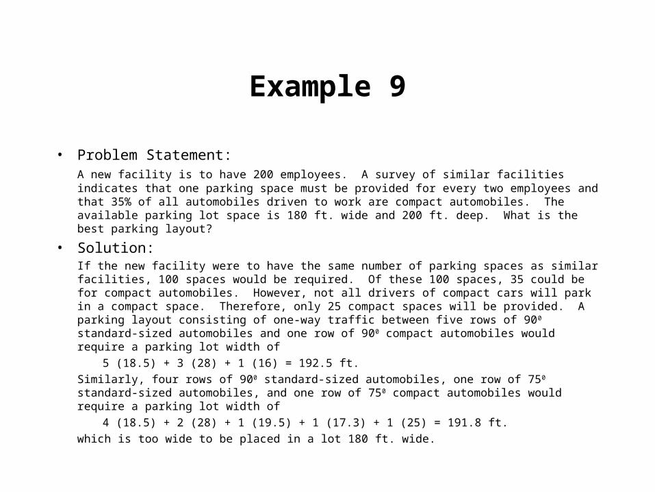
• Problem Statement:A new facility is to have 200 employees. A survey of similar facilities indicates that one parking space must be provided for every two employees and that 35% of all automobiles driven to work are compact automobiles. The available parking lot space is 180 ft. wide and 200 ft. deep. What is the best parking layout?
• Solution:If the new facility were to have the same number of parking spaces as similar facilities, 100 spaces would be required. Of these 100 spaces, 35 could be for compact automobiles. However, not all drivers of compact cars will park in a compact space. Therefore, only 25 compact spaces will be provided. A parking layout consisting of one-way traffic between five rows of 900 standard-sized automobiles and one row of 900 compact automobiles would require a parking lot width of
5 (18.5) + 3 (28) + 1 (16) = 192.5 ft.
Similarly, four rows of 900 standard-sized automobiles, one row of 750 standard-sized automobiles, and one row of 750 compact automobiles would require a parking lot width of
4 (18.5) + 2 (28) + 1 (19.5) + 1 (17.3) + 1 (25) = 191.8 ft.
which is too wide to be placed in a lot 180 ft. wide.

Example 9 (cont.)
Replacing the 750 aisle with a 600 aisle still requires 184.7 ft. Four rows of 900 standard-sized automobiles, one row of 450 standard-sized automobiles, and one row of 450 compact automobiles requires a parking lot width of
4 (18.5) + 2 (28.0) + 1 (17.5) + 1 (17.0) + 1 (13.0) = 177.5 ft.
This configuration will be utilized.
Leaving 24 ft. for two-way cross-aisle traffic at the front of the lot and 14 ft. for one-way cross-aisle traffic at the rear of the lot, the 900 standard-sized automobile rows can each accommodate
200 24 14
8 519
( )
.automobiles
The last 900 standard-sized row does not require the 14 ft. one-way cross-aisle. Therefore, it accommodates
200 24
8 520
.automobiles
The 450 standard-sized row can accommodate
200 24 14
12 013
( )
.automobiles

Example 9 (cont.)
The 450 compact automobile row is the first and does not require the 14.0 ft. one-way cross-aisle. It can accommodate
200 24
10 516
.automobiles
Hence, a total of
3 (19) + 20 + 13 + 16 = 106 automobiles
can be accommodated, with 15% being allocated to compact automobiles. The following Figure illustrates the plan for the parking lot.
If the compact automobile row is replaced by standard-sized automobiles, the lot still fits within the 180 ft. 200 ft. configuration and 104 cars may be accommodated. Therefore, a decision must be made regarding the advantages of providing compact automobile spaces versus not segmenting the parking lot.

Parking Lot for Example 9
19 Standard-sized automobiles (900)
19 Standard-sized automobiles (900)
20 Standard-sized automobiles (900)
19 Standard-sized automobiles (900)
13 Standard-sized automobiles (450)
16 Compact automobiles (450)