spacecraft design optimisation for demise and survivability

of 36

Spacecraft design optimisation for demise and survivability

Mirko Trisolinia*, Hugh G. Lewisa, Camilla Colombob

a Astronautics Research Group, University of Southampton, Southampton , SO17 1BJ, United Kingdom,

[email protected], [email protected] b Department of Aerospace Science and Technology, Politecnico di Milano, Via La Masa 34, 20133, Milan, Italy,

[email protected]

* Corresponding Author

Abstract

Among the mitigation measures introduced to cope with the space debris issue there is the de-orbiting of

decommissioned satellites. Guidelines for re-entering objects call for a ground casualty risk no higher than 10-4. To

comply with this requirement, satellites can be designed through a design-for-demise philosophy. Still, a spacecraft

designed to demise through the atmosphere has to survive the debris-populated space environment for many years.

The demisability and the survivability of a satellite can both be influenced by a set of common design choices such

as the material selection, the geometry definition, and the position of the components inside the spacecraft. Within

this context, two models have been developed to analyse the demise and the survivability of satellites. Given the

competing nature of the demisability and the survivability requirements, a multi-objective optimisation framework

was developed, with the aim to identify trade-off solutions for the preliminary design of satellites. As the problem is

nonlinear and involves the combination of continuous and discrete variables, classical derivative based approaches

are unsuited and a genetic algorithm was selected instead. The genetic algorithm uses the developed demisability and

survivability criteria as the fitness functions of the multi-objective algorithm. The paper presents a test case, which

considers the preliminary optimisation of tanks in terms of material, geometry, location, and number of tanks for a

representative Earth observation mission. The configuration of the external structure of the spacecraft is fixed. Tanks

were selected because they are sensitive to both design requirements: they represent critical components in the

demise process and impact damage can cause the loss of the mission because of leaking and ruptures. The results

present the possible trade off solutions, constituting the Pareto front obtained from the multi-objective optimisation.

Keywords: design-for-demise, survivability, multi-objective optimisation, tanks

Nomenclature

a Semi-major axis Km

A Area m2

C Speed of sound m/s

CD Drag coefficient

CF Correction factor for component mutual

shielding

Cm Heat capacity J/Kg-K

D Diameter m

d Lateral size of a component in the impact

plane

m

E0 Maximum allowed displacement from the

nominal ground track at the equator

Km

�̅�𝑞 Motion and shape averaged shape factor

for heat flux predictions

G Universal gravitational constant

g Polar component of the gravitational

acceleration

m/s2

g0 Gravitational acceleration at sea level m/s2

gR Radial component of the gravitational

acceleration

m/s2

h Altitude Km

hf Heat of fusion J/kg

Isp Specific impulse s

mailto:[email protected]



of 36

K1 Factor to account for the additional tank

volume for the pressuring gas

K2 Factor to account for the separation

between two tanks

l Distance between two tanks m

L Side length of the spacecraft m

L Length m

m Mass Kg

ME Earth’s mass, 5.97×1024 Kg

N Total number of spacecraft components

nt Number of tanks

Pp Penetration probability

r Radius m

RE Earth’s radius, 6371800 m

rn Nose radius m

S Cross-section of the spacecraft m2

s Stand-off distance m

SF Tank pressure safety factor

t Thickness m

tm Mission duration years

Tm Melting temperature K

V Velocity m/s

v Volume m3

α Cone ejecta spread angle °

γ Flight path angle °

ε Emissivity

θ Impact angle °

λ Longitude °

ρ Density Kg/m3

σ Stefan-Boltzmann constant, 5.67×10-8 W/m2/K4

σu Ultimate tensile strength MPa

σy Yield strength MPa

φ Latitude °

Debris flux 1/m2/yr

χ Heading angle °

ω Angular velocity °/s

Subscripts

0 Nominal orbit

1 Start orbit for the Hohmann transfer

2 Final orbit of the Hohmann transfer

atm Atmosphere

BLE Relative to the probability of penetrating

an internal component

C Relative to the critical diameter

comp Relative to the probability of impacting a

component after a first impact on the

vulnerable zone

decay Relative to decaying correction

manoeuvres

disp Relative to disposal manoeuvres

e Earth

ejecta Relative to the debris cone produced after

impact

f Fuel

fin Final condition

of 36

in Initial condition

inc Relative to inclination change manoeuvres

inj Relative to orbit injection errors

mat Material

p Debris particle

s Spacecraft

sec Relative to secular variations of the orbital

parameters

struct Relative to the impact on the external

structure inside the vulnerable zone

t Tank

target Target component of the impact

probability analysis

tot Total

VZ Relative to the vulnerable zone

w Wall

Abbreviation

DAS Debris Assessment Software

LMF Liquid Mass Fraction

BLE Ballistic Limit Equation

SRL Schafer-Ryan-Lambert

NSGA Non-dominated Sorting Genetic

Algorithm

PNP Probability of no-penetration

1 Introduction

In the past two decades, the attention towards a more sustainable use of outer space has increased steadily. The

major space-faring nations and international committees have proposed a series of debris mitigation measures [1, 2]

to protect the space environment. Among these mitigation measures, the de-orbiting of spacecraft at the end of their

operational life is recommended in order to reduce the risk of collisions in orbit.

However, re-entering spacecraft can pose a risk to people and property on the ground. Consequently, the re-entry

of disposed spacecraft needs to be analysed and its compliancy with international regulations has to be assessed. In

particular, the casualty risk for people on the ground related to the re-entry of a spacecraft needs to be below the limit

of 10-4 if an uncontrolled re-entry strategy is to be adopted [3, 4]. A possible strategy to limit the ground casualty risk

is to use a design-for-demise philosophy, where most (if not all) of the spacecraft will not survive the re-entry

process. The implementation of design for demise strategies [5-7] may favour the selection of uncontrolled re-entry

disposal options over controlled ones, leading to a simpler and cheaper alternative for the disposal of a satellite at the

end of its operational life [6, 7]. However, a spacecraft designed for demise still has to survive the space environment

for many years. As a large number of space debris and meteoroids populates the space around the Earth, a spacecraft

can suffer impacts from these particles, which can be extremely dangerous, damaging the spacecraft or even causing

the complete loss of the mission [8-10]. This means that the spacecraft design has also to comply with the

requirements arising from the survivability against debris impacts.

The demisability and survivability of a spacecraft are both influenced by a set of common design choices, such as

the material of the structure, its shape, dimension and position inside the spacecraft. It is important to consider such

design choices and how they influence the mission’s survivability and demisability from the early stages of the

mission design process [7]. In fact, taking into account these requirements at a later stage of the mission may cause

an inadequate integration of these design solutions, leading to a delayed deployment of the mission and to an

increased cost of the project. On the other hand, an early consideration of such requirements can favour cheaper

options such as the uncontrolled re-entry of the satellite, whilst maintaining the necessary survivability and, thus, the

mission reliability.

With these considerations, two models have been developed [11] to assess the demisability and the survivability

of simplified mission designs as a function of different design parameters. Two criteria are presented to evaluate the

degree of demisability and survivability of a spacecraft configuration. Such an analysis can be carried out on many

different kinds of missions, provided that they can be disposed through atmospheric re-entry and they experience

impacts from debris particles during their operational life. These characteristics are common to a variety of missions;

of 36

however, it was decided to focus the current analysis on Earth observation and remote sensing missions. Many of

these missions exploit sun-synchronous orbits due to their favourable characteristics, where a spacecraft passes over

any given point of the Earth’s surface at the same local solar time. Because of their appealing features, sun-

synchronous orbits have high commercial value. Alongside their value from the commercial standpoint, they are also

interesting for a combined survivability and demisability analysis. Sun-synchronous missions can in fact be disposed

through atmospheric re-entry. They are also subject to very high debris fluxes [12] making them a perfect candidate

for the purpose of this study.

Given the competing nature of the demisability and survivability requirements, a multi-objective optimisation

framework has been developed, with the aim to find trade-off solutions for the preliminary design of satellites. As

the problem is nonlinear and involves the combination of continuous and discrete variables, classical derivative

based approaches are unsuited and a genetic algorithm was selected instead. The genetic algorithm uses the

previously described demise and survivability criteria as the fitness functions of the multi-objective algorithm.

The paper presents a test case, which considers the preliminary optimisation of tanks in terms of material,

geometry, location, and number of tanks for representative sun-synchronous missions. The configuration of the

external structure of the spacecraft was fixed. Tanks were selected because they are interesting for both the

survivability and the demisability. They represent critical components in the demisability analysis as they usually

survive the atmospheric re-entry. They are also components that need particular protection from the impact against

space debris because the impact with debris particles can cause leaking or ruptures, which can compromise the

mission success. Different configurations were analysed as a function of the characteristics of the tank assembly and

of the mission itself, such as the mission duration and the mass class of the spacecraft. The results are presented in

the form of Pareto fronts, which represent the different possible trade-off solutions.

2 Demisability and Survivability Models

In order to carry out a combined demisability and survivability analysis of a spacecraft configuration it was

necessary to develop two models [11, 13-15]. One model allows the analysis of the atmospheric re-entry of a

simplified spacecraft configuration in order to evaluate its demisability. The other model carries out a debris impact

analysis and returns the penetration probability of the satellite as a measure of its survivability. As these two models

need to be implemented into an optimisation framework, much effort was made to maintain a comparable level of

detail and computational time between them.

2.1 Demisability model

The demisability model consists of an object-oriented code [16-18]. The main features of this type of code is the

fast simulation of the re-entry of a spacecraft that is schematised using primitive shapes such as spheres, cubes,

cylinders, and flat plates. These primitive shapes are used as a simplified representation of both the main spacecraft

structure and internal components. The different parts of the spacecraft are defined in a hierarchical fashion. The first

level is constituted by the main spacecraft structure (commonly referred as the parent object). Here the overall

spacecraft mass and dimensions are defined, as well as the solar panels area. The second level defines the external

panels of the main structure. This gives the opportunity to the user to specify different characteristics for the external

panels, such as the material, the thickness, and the type of panel (e.g. honeycomb sandwich panel). The third level

defines the main internal components such as tanks and reaction wheels. An additional level can also be used for the

definition of sub-components like battery cells.

The main structure of the code is represented in Figure 1. First, the software requires a set of inputs from the user,

which has to provide the initial conditions of the re-entry trajectory in the form of longitude, latitude, altitude,

relative velocity, flight path angle, and heading angle. The second required input from the user is the spacecraft

configuration. This is a file describing the characteristics of each component in the configuration. An example of the

structure of such file is represented in Table 1. Additionally, the user can specify the integration options, such as the

time step, and the relative and absolute tolerances.

Table 1: Example of spacecraft configuration to be provided to the software.

ID Name Parent Shape Mass (kg) Length (m) Radius (m) Width (m) Height (m) Quantity

0 Spacecraft n/a Box 2000 3.5 n/a 1.5 1.5 1

1 Tank 0 Sphere 15 n/a 0.55 n/a n/a 1

2 BattBox 0 Box 5 0.6 n/a 0.5 0.4 1

3 BattCell 2 Box 1 0.1 n/a 0.05 0.05 20

… … … … … … … … … …

of 36

Figure 1: Flow diagram of the main structure of the re-entry software.

After the initialisation is complete, the trajectory of the parent object is simulated. This first part of the simulation

carries on until the main break-up altitude is reached and only the parent structure can interact with the external heat

flux. The internal components do not experience any heat load during this phase. The break-up altitude is user-

defined but the default value is set to 78 km, which is the standard value used in most destructive re-entry software

[19]. During this first phase of the simulation, the software can take into account the occurrence of some specific

events, such as the detachment of the solar panels or the external panels of the main structure. It is considered that

the solar panels separate from the main structure at a fixed altitude, equal to 95 km [20, 21]. When this altitude is

reached, the solar panels are simply removed from the simulation, with the consequent change in the aerodynamics

of the structure, as the area of the solar panels is not considered anymore in the contribution to the average cross-

section of the spacecraft. The re-entry of the solar panels after detachment is not simulated, as they are considered to

always demise. The detachment of the external panels of the structure is instead triggered by the temperature of the

panels themselves. Once the temperature reaches the melting the temperature of the panel material, the panel is

considered to detach [22]. If an internal component is attached to the panel, also the component is considered to

detach from the main structure. At this point, the detachment conditions for each detached panel and component are

stored for a later use and the mass of the spacecraft is updated accordingly. The first part of the simulation ends with

of 36

the main spacecraft reaching the break-up altitude. At this point, the break-up state is also stored, as it will be used as

the initial state for all the internal components released at break-up. After the break-up event, the parent spacecraft is

removed and the re-entry of the internal components and of the external panels is simulated. To each component is

associated an initial condition that is the previously stored detachment conditions.

Figure 2: Flow diagram for the procedure used in the integration of the re-entry trajectory.

When the re-entry of the component has to be simulated, its initial condition is loaded. The simulation continues

until the component reaches the ground, or it is completely demised, or its energy is below the threshold of 15 J [3].

When one of these events occurs, the simulation is stopped and the re-entry output is stored. We store the final mass,

cross-section, landing location and impact energy of each surviving object, and the demise altitude of each demised

object. The simulation procedure is repeated for each internal component and external panel. The procedure followed

for the integration of the trajectory of the main spacecraft and the internal components is summarised in Figure 2.

The trajectory is simulated with a three degree-of-freedom ballistic dynamics, where the computation of the attitude

motion of the objects is neglected and the attitude motion is predefined and assumed random tumbling. The Earth’s

atmosphere is modelled using the 1976 U.S Standard Atmosphere [23]. The Earth’s gravitational acceleration is

modelled using a zonal harmonic gravity model up to degree four [24]. The radial and polar contributions to the

gravity vector can be expressed as

2 3

2 3

2 3

4

4 2

4

31 [3sin 1] 2 [5sin 3sin ]

2

5[35sin 30sin 3]

8

E E E

R

E

GMg

r r

R RJ

J

rJ

R

r

− − − −

− −

= −

+

(1)

of 36

2

2

3

2

2

4

2 2

1[5sin 1]

2

5[7s 1

3

in ]6

sin cosE E E

E

G RM RJ J

rr

r

R

r

J

g

+ −

+ −

=

(2)

where gR and gϕ are the radial and polar components of the gravitational acceleration. G is the universal

gravitational constant, ME is the mass of the Earth, RE is the equatorial radius of the Earth, r is the distance between

the satellite and the centre of the Earth, is the latitude. Finally, the Jks (k = 2, 3, 4) are the zonal harmonic

coefficients, which take into account the effect of the Earth’s oblateness and not uniform mass distribution.

Alongside the gravitational forces, the aerodynamic forces are needed in order to predict the trajectory of the

spacecraft and its components. The aerodynamic force acting on the object during the re-entry can be expressed as

21

2D DF V S C= (3)

where ρ is the air density, V is the air velocity, S is the cross section and CD is the drag coefficient. The drag

coefficient is computed using averages over the motion and shape of the object [25-27]. In addition, drag coefficients

for both free-molecular and continuum regimes are taken into account. During its descent, in fact, the spacecraft

encounters very rarefied air at high altitude such that the continuum flow model cannot be adopted and a free-

molecular approximation needs to be used. The free-molecular and continuum drag coefficient for each elementary

shape are summarised in Table 2.

Table 2: Free-molecular and continuum drag coefficients.

Shape Free-molecular CD Continuum CD Reference area

Sphere 2.0 0.92 D2 / 4

Box 1.0 (Ax + Ay + Az) / Ay 0.46 (Ax + Ay + Az) / Ay Ay

Cylinder 1.57+0.785 D / L 0.7198+0.326 D / L D L

Flat Plate 1.03 0.46 A

where D is the diameter of the sphere or the cylinder, L is the length of the cylinder, and Ax, Ay, and Az are the

areas of the sides of the box. The areas are ordered such that Ax ≥ Ay ≥ Az.

Similarly to the aerodynamics, even the aerothermodynamics is taken into account using motion and shape

averaged coefficients. In general, the heat flux on an object is computed as follows

av q refq F q= (4)

Where �̇�𝑎𝑣 is the average heat load on the object in W/m2, �̅�𝑞 is the averaging factor depending on the shape of

the object, its motion, and the re-entry regime (i.e. free-molecular or continuum), and �̇�𝑟𝑒𝑓 is the reference heat load

on the object. The reference heat load is different from the free-molecular and the continuum case. In the first case, is

represented by the heat rate on a flat plate perpendicular to the free-stream flow that is

3

0 011356.61556

fm

rem

a Vq

=

(5)

where a is the thermal accommodation coefficient. For metallic material the accommodation coefficient is

usually around 0.9, which was adopted as the constant in the current analysis [27]. ρ0 is the free-stream density and

V0 is the free-stream velocity. In the continuum case, instead, the reference heat load is the heat flux at the stagnation

point of a sphere, which is the Detra, Kemp and Riddel (DKR) correlation [27, 28]

300

3.15

8 0 00.30481.99876 10

7924.8

cont s w

ref

n SL s w

V h hq

r h h

− =

− (6)

of 36

where rn is the curvature radius at stagnation point, and ρSL is the air density at sea-level. hs is the stagnation point

enthalpy, hw is the wall enthalpy and hw300 is the wall enthalpy at 300 K. The averaging factors for the computation of

the heat flux are summarised in Table 3.

Table 3: Free-molecular and continuum averaging factors for the heat load computation.

Shape Free-molecular �̅�𝑞 Continuum �̅�𝑞 Reference area

Sphere 0.255 0.345 D2

Box

0.1275 / 0.785

0.5

eq eq

eq eq

box

wet

D L YD L

Z

A

+

+

0.179 0.1615 /

0.333

eq eq

eq eq

box

wet

D LD L

B

A

+

+

box

wetA

Cylinder 0.255 / 1.57

2 /

D L Y Z

D L

+ +

+

0.358 0.323 / 0.666

2 /

D L B

D L

+ +

+

2

DD L

+

Flat Plate 0.255

,

0.233d eq

wet

fp

wet

A

A fp

wetA

To compute the box shape factors an equivalent cylinder has been used [27]. 𝐷𝑒𝑞 = 2 ∙ √𝑊 ∙ 𝐻 is the equivalent

diameter and Leq = L is the equivalent length, with L, W, and H being the length, width and height of the box. 𝐴𝑤𝑒𝑡𝑏𝑜𝑥 =

2 ∙ (𝐿𝑊 + 𝐿𝐻 +𝑊𝐻)Awet is the external surface of the box, and Y, Z, and B are values dependent on the Mach

number and can be extracted from plots available at [25]. 𝐴𝑤𝑒𝑡𝑓𝑝

is the external area of the flat plate, and 𝐴𝑤𝑒𝑡𝑑,𝑒𝑞

is the

external area of an equivalent disk with an equivalent diameter of Deq = W/2.

The trajectory is described by a set of three degree-of-freedom equations of motion, where the spacecraft is

treated as a material point and its attitude motion is established a priori. As previously described, the aerodynamics

and aerothermodynamics are thus expressed using motion and shape averaged coefficients. As the aerodynamic

forces are due to the motion of the vehicle relative to the atmosphere of the planet, a reference frame fixed with the

atmosphere is required to determine the aerodynamics loads on the vehicle. Since a planet's atmosphere rotates with

it, it is possible to define a planet-fixed reference frame in order to express the equations of the atmospheric flight

(Figure 3).

Figure 3: Planet fixed (SXYZ) and local horizon (oxyz) frames [24].

The complete set of equations of motion is summarised in Eqs. (7).

of 36

( )

( )

2

2

2

sin

cos cos

cos sin

cos

/ sin cos cos cos cos cos sin sin cos

sin sin sin cos 2cos sin tan tan cos cos sin

cos cos cos

cos cos sin cos

D R

R

r V

V

r

V

r

V F m g g r

gV r

r V V

ggV r

r V V

=

=

=

= − + − − −

= + + − −

= + + + ( )cos sin cos sin cos cos 2 sin cosV

+ +

(7)

where m is the mass of the spacecraft, and V is the velocity of the spacecraft relative to the atmosphere. is the

flight path angle, is the heading angle, λ is the longitude, and ω is the Earth’s angular velocity. Finally, FD is the

drag force, which is computed using Eq. (3).

While the temperature of the object is below the melting temperature of the material, the heat load increases the

object temperature. We use a lumped mass schematisation where the object temperature is considered uniform. The

temperature variation can be expressed as

( )

4

,

w w

av w

p m

dT Aq T

dt m t C = − (8)

where Tw is the wall temperature, Aw is the wetted area (external area of the object), m is the mass of the object

and Cp,m is the specific heat at constant pressure. �̇�𝑎𝑣is the heat flux already adjusted with the shape and attitude

dependant averaging factors. krad is a coefficient that takes into account the heat re-radiation, ε is the emissivity of the

material, and σ is the Stefan-Boltzman constant. Once the melting temperature is reached, the object starts melting

and losing mass at a rate that is proportional to the net heat flux on the object and the heat of fusion of the material.

4w

av w

m

Admq T

dt h = − − (9)

where hm is the heat of fusion of the material. The material database used is the one available in the NASA Debris

Assessment Software (DAS) [17] and integrated with data from [29].

2.2 Survivability model

The survivability model analyses the satellite resistance against the impacts of untraceable space debris and

meteoroids. Standard vulnerability analysis software relies on ray tracing method in order to predict the damage on

spacecraft panels and internal components. Such methods are computationally expensive and require many

simulations in order to have a statistically meaningful result, as the impact point of each particle is randomly

generated. We here describe a novel methodology that uses a probabilistic approach capable of computing the

vulnerability of a spacecraft configuration, avoiding ray tracing methods. The method is based on the concept of

vulnerable zone. The vulnerable zone concept is associated to the vulnerability of the internal components of a

spacecraft. In fact, it is defined as the area on the external structure of the spacecraft that, if impacted, can lead to an

impact also on the component considered. In a simpler fashion, if a space debris impacts on the vulnerable zone of a

component, than it also has the possibility to impact such component. The outline of the main characteristics of the

software is summarised in the flow diagram of Figure 9.

of 36

Figure 4: Flow diagram of the main structure of the survivability software.

The procedure involves representing the spacecraft structure with a panelised schematization of its outer structure

and using simple shapes for the internal components. To each panel and object, we assign a material selected from a

predefined library and geometrical properties such as the type of shielding, the wall thickness, etc.

Figure 5: Vector flux elements

Beside the geometrical schematization of the satellite, a representation of the space environment is needed. This

is obtained using the European Space Agency (ESA) state of the art software MASTER-2009 [30] that provides a

START

Load mission scenario and geometry

Load MASTER flux data

Compute vector flux elements

Compute vulnerable zone characteristics

Compute shields properties

Compute external structure vulnerability

Compute component vulnerability

Last component?

Compute overall vulnerability

END

Store shields properties

Store vulnerable zones properties

Store survivability results

Load shield and V.Z. properties

Yes

No

of 36

description of the debris environment via flux predictions on user defined target orbit. MASTER-2009 provides a set

of 2D and 3D flux distributions as a function of the impact azimuth, impact elevation, impact velocity, and particle

diameter. The next step consists in schematizing the debris environment around the satellite using vector flux

elements [11]. The space around the satellite is subdivided in a set of angular sectors and to each sector is associated

a vector flux element containing the weighted average of the impact flux, impact direction, impact velocity, and

impact diameter [11] (Figure 5). The next step consists in computing the characteristics of the vulnerable zones

associated to each internal component. In general, an impact will be oblique (i.e. the angle between the spacecraft

face and the impact velocity is not 90 degrees) resulting in two different debris clouds being produced after the

impact [31, 32]. One cloud exits almost perpendicularly to the impacted wall, the normal debris cloud. The second

cloud closely follows the direction of the projectile and is referred to as the in-line debris cloud (see Figure 6). We

take into account the clouds assuming that the debris belonging to the two clouds are contained inside conic surfaces

so that they can be modelled using just the direction of the cone axis and the spread angle of the cone (Figure 6).

Figure 6: Secondary ejecta clouds characteristics.

The geometry of the cones can be expressed as a function of the impact characteristics (impact velocity, impact

angle, particle diameter and wall material) as follows [31, 32]:

( )

( )

( )

0.4780.086

0.5861

0.1950.907

0.3942

0.3451.096

0.738

1

0.00.049

2

0.471 cos

1.318 cos

tan 0.471 cos

tan 1.556

p

p

p

p

p

p

p

p

V t

C D

V t

C D

V t

C D

V t

C D

−−

−−

=

=

=

=

( )

54

1.134cos

(10)

where t is the shield thickness, Dp is the particle diameter, Vp is the particle velocity, and C is the speed of sound

in the shield material. θ is the impact angle, θ1 is the normal cloud axis, θ2 is the inline cloud direction, ψ1 is the

cone aperture of the normal cloud, and ψ2 is the cone aperture of the inline cloud. These equations have been

developed for impacts on Whipple shields and for a range of impact angles (θ) between 30 and 75 degrees. However,

it is here assumed that the validity of the equations can be extended to the entire range of impact angles and to other

shielding configurations such as honeycomb sandwich panels [9]. The vulnerable zone [9] is defined as the area on

the external structure of the spacecraft that, if impacted, can lead to an impact also on the component considered.

Any impact of a particle onto this area generate fragments that may hit the component in question, with a probability

that depends on the impact parameters, the satellite structure and the stand-off distance of the component from the

structure wall. The lateral extent of the vulnerable zone is expressed as

of 36

( ),2 2 tan 0.5VZ max target p maxR s d D = + +

(11)

where (Figure 7) 2RVZ is the lateral extension of the vulnerable zone, s is the spacing between the structure wall

and the component face (stand-off distance), dtarget is the lateral size of the considered component, Dp,max is the

maximum projectile diameter, and αmax is the maximum ejection angle. To compute αmax, a simplification of Eqs.

(10) is adopted as it is suggested in [9]. It is assumed that the ejection and spread angles are only a function of the

impact angle θ and that all the other parameters can be absorbed by a constant factor giving:

( ) 2

22

= + (12)

The maximum ejection angle is then αmax = 63.15º.

Figure 7: Vulnerable zone extent representation.

The parameter Dp,max is a user defined value of the projectile diameter that takes into account the contribution of

the particle to the impact probability. Suggested values for Dp.max in [9] are 10 mm for vulnerable components and 20

mm for component with higher impact resistance. An example of vulnerable zones as computed by the described

procedure is presented in Figure 8.

Figure 8: Vulnerable zones of a cylinder projected onto the faces of a cubic structure (closest faces).

After the computation of the vulnerable zones properties, the software automatically detects the characteristics of

the shielding, storing all the data that are later necessary for the computation of the probability of penetration. Such

data includes the type of panel of the external structure (i.e. single plate or sandwich panel), the thickness of panels,

their material, the material of the target object, its thickness, its distance from the respective vulnerable zones, and all

the components that can possibly shield the target object.

of 36

Once the preliminary operations are terminated, the software analyses the vulnerability of the external structure

of the spacecraft. The procedure followed is outlined in the flow diagram of Figure 9.

Figure 9: Flow diagram for the vulnerability computation of the external structure.

Once the vector flux elements are computed, the areas of the spacecraft that are susceptible to particle impacts can

be determined using a visibility role. Considering the object to be represented by a set F of faces and a vector flux

elements with a velocity vector vi, to verify if particles can impact one of the panels in the set F we check the velocity

vector vi with respect to the panel normal nj using Eq. (13).

0 j in v (13)

All the faces F representing the component are checked against all the vector flux elements following the same

visibility role. Then we can compute the probability of such impact. Assuming that debris impact events are

probabilistic independent [33], it is possible to use a Poisson statistics to compute the impact probability.

( ), 1 exp j

i m

j iimp A tP ⊥− = − (14)

where 𝑃𝑖𝑚𝑝𝑗,𝑖

is the probability of an impact on the j-th vulnerable zone by the i-th vector flux element. φi is the i-th

vector flux, 𝐴⊥𝑗

is the projected area of the j-th face considered, and tm is the mission time in years. It is then necessary

to compute the penetration probability on the panels. Ballistic limit equations [34] are used to compute the critical

diameter using the velocity and direction associated with the vector flux elements together with the geometric and

material characteristics of the panels. Once computed the critical diameter for the i-th vector flux onto the j-th the

penetration probability is given by

( ),

, 1 exp j

C i m

j ip A tP ⊥− = − (15)

where φC,i is the particle flux with a diameter greater than the computed critical diameter. With the presented

methodology, the computation of the critical flux for each vector flux element replaces the direct sampling of the debris

particles. The critical flux can be extracted from the distribution of the cumulative flux vs diameter provided by

MASTER-2009 (Figure 10)

START

END

Vector flux element impacts

panel?

Compute critical diameter

Compute critical flux

Compute panel vulnerability

Compute vulnerability

Store panel vulnerability

Load panels vulnerability

No

Yes

of 36

Figure 10: Critical flux computation methodology

As the global distribution of cumulative flux vs diameter is used, the flux extracted is the overall flux for the entire

range of azimuth and elevation, it thus cannot be directly used to compute the penetration probability relative to one

of the vector flux elements. In fact, to each vector flux is associated a value of the particle flux that is dependent upon

the directionality, i.e., impact elevation and impact azimuth, which is a fraction of the total flux. It is here assumed that

the distribution of the particles diameter is uniform with respect to the impact direction. With this assumption, the

critical flux associated to a vector flux element is considered as a fraction of the overall critical flux. If φTOT is the total

debris flux and C is the overall critical flux computed, the critical flux relative to the considered vector flux element

can be expressed as

,

C

C i i

TOT

= (16)

Finally, the penetration probability on the external structure can be computed as follows

( ),

1 1

1 1panels fluxes

p

N N

j ip

j i

P P= =

= − − (17)

with Nfluxes total number of vector fluxes elements and Npanels total number of panels composing the structure.

After the analysis of the external structure is completed, the internal components are considered. The procedure

followed for the internal components is similar to the one for the external structure; however, it directly involves the

use of the vulnerable zones. The procedure is schematised in the flow diagram of Figure 11.

of 36

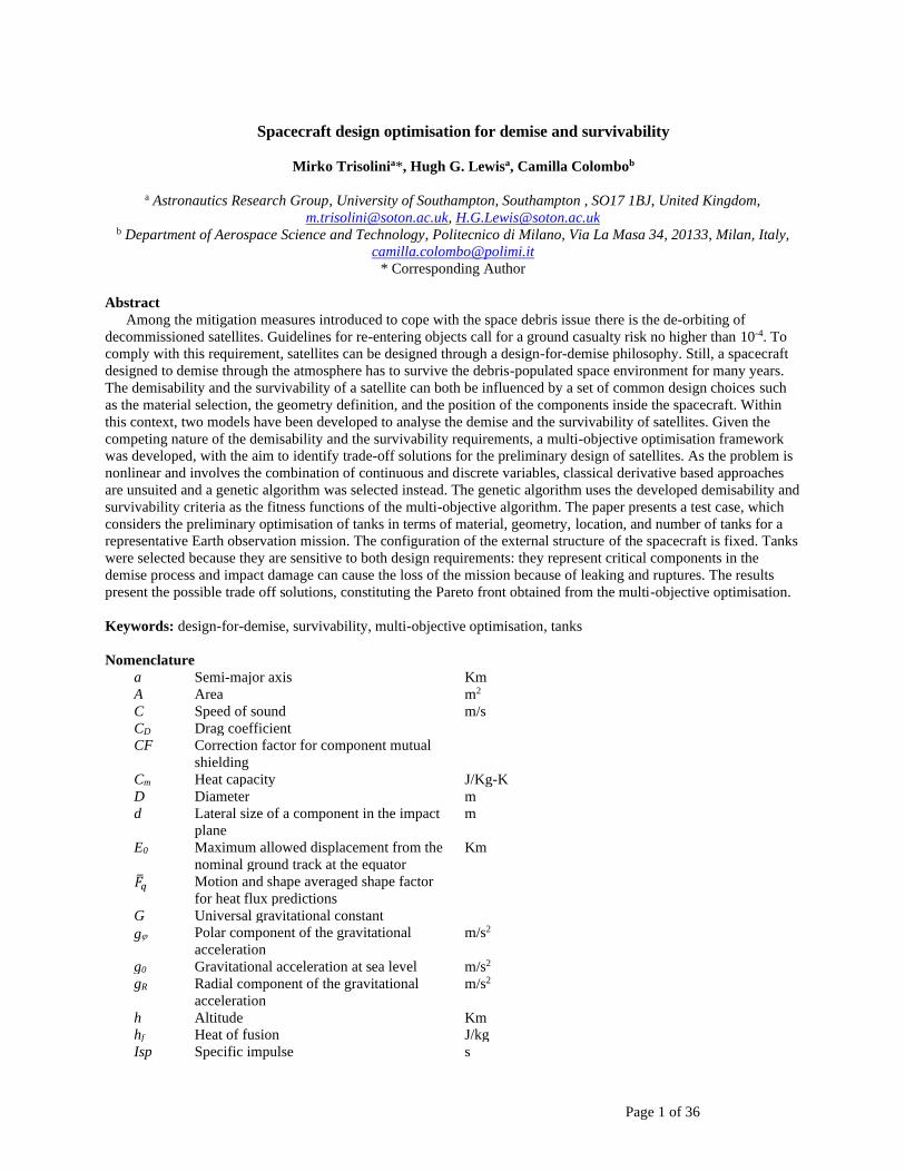
Figure 11: Flow diagram for the vulnerability computation of an internal component.

When a debris particle with sufficient size and velocity impacts onto the outer structure of the spacecraft, a

secondary debris cloud is usually generated. Particles belonging to this debris cloud can still impact internal

components and damage them. It is thus necessary to evaluate the probability that such secondary debris penetrate

the inner components. The vulnerability of an internal component can be evaluated as the product of three different

probabilities:

p struct comp BLEP P P P= (18)

where Pstruct is the probability of space debris impacting the spacecraft external structure inside the vulnerable

zone assigned to the specific spacecraft component; Pcomp is the probability that the downrange fragment cloud will

hit the component; and PBLE is the probability that the projectile in this cloud perforates the component wall.

Consequently, the entire procedure consists in computing the different terms of Eq. (18). The probability of having

an impact on the vulnerable zone is similar to the one for the external panels expressed by Eq. (14). The first

contribution in the equation 𝑃𝑠𝑡𝑟𝑢𝑐𝑡𝑗,𝑖

can thus be computed as

( ),

,1 expj i j

struct i VZ mP S t ⊥= − − (19)

where 𝑃𝑠𝑡𝑟𝑢𝑐𝑡𝑗,𝑖

is the probability of an impact on the j-th vulnerable zone by the i-th vector flux element. i is the i-

th vector flux, 𝑆𝑉𝑍,⊥𝑗

is the projected area of the j-th vulnerable zone corresponding to the component; and tm is the

mission time in years. A particle impacting the vulnerable zone or the resulting debris cloud will not necessarily

impact the inner component associated with it. It is thus necessary to take into account the probability that an impact

START

Vector flux element impacts

panel?

Compute impact probability on V.Z. (Pstruct)

Compute probability of impacting the component (Pcomp)

Compute penetration probability (PBLE)

Compute critical diameter

Compute critical flux

Ballistic impact?

Compute ballistic correction factor

Compute hypervelocity correction factor

Compute panel vulnerability Store panel vulnerability

Compute object vulnerability Load panels vulnerability

END

Next vector flux element

Next vulnerable zone

Yes

Yes

No

No

of 36

on the vulnerable zone will subsequently cause an impact on the component itself. This is taken into account by the

second term on the right end side of Eq. (18). This term (𝑃𝑐𝑜𝑚𝑝𝑗,𝑖

) depends on the type of impact: if the impact occurs

in the hypersonic regime, secondary debris clouds will form, whereas if the impact is in the ballistic regime the

projectile will pass almost intact through the outer structure. It is thus necessary to distinguish between these two

situations. In the hypervelocity regime the probability to impact the component is the ratio between the extent of the

ejecta in the component plane and the vulnerable zone of the component [9] and can be expressed as:

,

2

ejectaj i

comp j

VZ

dP

R= (20)

where 𝑃𝑐𝑜𝑚𝑝𝑗,𝑖

is the probability that the i-th vector flux element, which has already impacted the j-th vulnerable

zone, will hit the component considered. 𝑅𝑉𝑍𝑗

is the extent of the j-th vulnerable zone in the target plane. dejecta is the

extent of the debris ejecta at the target plane and is computed as follows:

( ),2 tan 1/ 2j i

ejecta max j targetd s d == +

(21)

where sj is the stand-off distance between the component and the external wall to which the j-th vulnerable area is

associated, and αmax(θj,i) is the maximum ejection angle associated with the i-th vector flux element impacting on the

i-th vulnerable zone, and can be computed with Eq. (12). In case of an impact in the ballistic regime, only the size of

the projectile needs to be considered, as no fragmentation occurs.

,

,

2

j i

p targetj i

comp j

VZ

d dP

R

+= (22)

where 𝑑𝑝𝑗,𝑖

is the particle diameter relative to the i-th vector flux element impacting on the j-th vulnerable zone.

This value is associated to each vector flux element and is extracted from the debris flux distributions obtained with

MASTER-2009 as the most probable particle diameter for the i-th vector flux element. For the scatter regime, a

linear interpolation between the ballistic and hypervelocity regime is adopted.

The described procedure still fails to take into account the mutual shielding between components that is the

capacity of a component to prevent another one from being hit by the debris particles. In order to take into account

such phenomenon, an approach using correction factors has been introduced. Given the different nature of the

impacts in the hypervelocity and in the ballistic regime, two correction factors are used. In the case of the

hypervelocity regime, the correction factor accounts for the fraction of the extent of the debris ejecta (Eq. (20)) that

can be covered by the shielding components. The expression of the correction factor for the i-th vector flux elements

is as follows:

,

1 ,

,1

sn

target

shield i

k shield k

hyp i

ejecta

sd

sCF

d

=

= −

(23)

where ns is the number of shielding components between the external face and the target component. dshield,k is the

extent of the k-th shielding component, starget is the minimum distance of the target component from the external face,

sshield,k is the minimum distance between the k-th shielding component and the external face, and dejecta is defined as in

Eq. (21). The correction factor takes into account the projection of the extent of each shielding component onto the

target plane (Figure 12). In case the extent of dshield exceeds the boundaries of the target plane, dshield is clipped with

the target plane, thus only considering the portion of the target projection that is actually inside the spacecraft

structure.

of 36

Figure 12: Representation of shielding component contribution to the correction factor.

If the correction factor is 1, no shielding is present, if is 0 the target component is not visible by the impactor. It is

possible to observe that the correction factor depends on the impact characteristics (i.e. impact angle); therefore, it

has to be computed for each vector flux element impacting the considered vulnerable zone, in case the impact is of

hypervelocity nature. In the case of the ballistic regime, the same approach cannot be used, as there is no ejecta

generation. Looking at Eq. (22), the impact probability in the ballistic regime depends only on the size of the particle

and on the extent of the target object. As the dimension of the particle cannot change, we can only act on the extent

of the target in order to correct the impact probability. In the case of a ballistic impact we thus use a corrected target

extent, which can be referred to as the visible target extent. Using an approach similar to the hypervelocity case, the

section of the shielding components is projected onto the target plane (Figure 13).

Figure 13: Perspective projection of a shielding component onto the target plane.

At this point, if the projections of the shielding components intersect the target component, they are subtracted

from the target components using Boolean operations (difference between sections).

( ), ,1 , ,, , , ,

sv i target shield shield k shield n

A A A A A= (24)

Where Av is the visible area of the target, Atarget is the target component section, and Ashield,k are the areas of the

shielding components projected onto the target plane. ¬ is the symbol for the Boolean NOT operator, which

corresponds to the difference between polygons. Again, whenever a projection of a shielding component has a

portion outside the target plane, it is clipped with the target plane itself. As lengths are used in the computation of the

impact probability, it is necessary to convert the visible area into a visible length (equivalent). The equivalent visible

length (dv,eq) is computed as follows:

,

2 /v eq v

d A = (25)

of 36

This expression corresponds to the diameter of an equivalent circle with area equal to the visible target area. The

ballistic correction factor can then be expressed as

,v eq

ball

target

dCF

d= (26)

Finally, the hypervelocity and the ballistic can be applied to the impact probabilities of Eqs. (27) and (28)

respectively as follows:

, ,

2

ejectaj i j i

comp hypj

VZ

dP CF

R=

(27)

,

,

2

j i

p ball targetj i

comp j

VZ

d CF dP

R

+ =

(28)

The last contribution in Eq. (18) comes from the computation of the penetration probability. The procedure is

analogous to the one described for the external structure, and the equation closely resemble Eq. (15).

( ),

, ,1 expj i j

BLE C i VZ mP S t ⊥= − − (29)

where 𝑃𝐵𝐿𝐸𝑗,𝑖

is the penetration probability for the j-th vector flux element on the component associated with the i-

the vulnerable zone, and C,i is the critical flux that is the flux associated to the value of the critical diameter

computed with ballistic limit equation. The adopted ballistic limit equation is the Schafer-Ryan-Lambert (SRL) [9,

34]. The SRL BLE is a triple-wall ballistic limit equation and can be used for both triple-wall and double wall-

configuration. The software uses this equation in a way that assumes the last wall of the shielding configuration is

always the face of the inner component considered, whereas the other walls represent the outer structure. The overall

penetration probability for a component can then be computed combining al the previous contributions as follows

( ), , ,

1 1

1 1panels fluxesN N

j i j i j i

p struct comp BLE

j i

P P P P= =

= − −

(30)

3 Sun-synchronous missions

As mentioned, for the presented analysis we are considering the optimisation of tank configurations of Earth

observation and remote sensing missions [35, 36]. These kinds of missions frequently exploit sun-synchronous orbits

and that is the reason why the current work focuses on these orbits. A sun-synchronous orbit is a Low Earth Orbit

(LEO) that combines altitude and inclination in order for the satellite to pass over any given point of the Earth’s

surface at the same local solar time, granting the satellite a view of the Earth’s surface at nearly the same

illumination angle and sunlight input. To estimate the size of the tank assembly it is necessary to compute the

amount of propellant needed for the mission through a delta-V budget. As sun-synchronous orbits are influenced by

atmospheric drag and by the non-uniformity of the Earth’s gravitational field, they require regular orbit correction

manoeuvres. They also need, as for most spacecraft, additional manoeuvres to correct orbit injection errors and to

perform disposal manoeuvres. The computation of the different contributions to the delta-V budget is described in

the following paragraph.

3.1 Delta-V budget

To estimate the tankage volume it is necessary to compute the amount of propellant needed by the spacecraft as a

function of the mission characteristics. The three main elements that contribute to the ΔV budget for the required

mission lifetime are the orbit maintenance, the launch injection errors, and the disposal manoeuvres.

Orbit maintenance manoeuvres are used to maintain the sun-synchronism of the orbit and to control the ground

track with a given accuracy. To do so, the orbital height and inclination need to be maintained within admissible

ranges. In LEO, atmospheric drag results in orbital decay, causing the semi-major axis and the orbit period to

decrease. The reduction in the semi-major axis δa and in the orbital period δτ for one orbit can be computed as

2

02 D

atm

s

SCa a

m = − (31)

of 36

3

s

aV

= (32)

where ρatm is the atmospheric density, S is the average cross section of the satellite, CD is the drag coefficient, ms is

the mass of the satellite, a0 is the nominal orbit semi-major axis, and Vs is the orbital velocity of the spacecraft. The

changes in the orbital height and period lead to changes in the ground track. Such variations can be controlled by

imposing a tolerance on the nominal ground track. When the spacecraft’s ground track reaches the prescribed

tolerance, a correction manoeuvre needs to be executed. To do so, the time difference from the nominal time at the

equator passage Δt0 needs to be computed:

0

e

t

= (33)

where ωe is the angular speed of the Earth and Δλ is the longitude displacement at equator passage and can be

expressed as:

02

e

E

r = (34)

re is the radius of the Earth, and E0 is the imposed tolerance on the displacement from the nominal orbit ground track

at the equator (equal to 0.7 km for this study). Using Eqs. (33) and (34) It is possible to compute the number of orbits

after which the equator crossing displacement reaches the prescribed limit as follows:

02 tk

= (35)

To control the ground track, the manoeuvre has to be executed every 2k orbits, leading to a variation in the orbit

semi-major axis (Δadecay) and orbital period (Δtdecay) of:

2

2

decay

decay

a k a

t k

=

= (36)

Δtdecay is also the time between the necessary orbit correction manoeuvres. The correction manoeuvre can be

computed with a Hohmann transfer:

2 1

,

1 1 2 2 1 2

2 21 1e e

decay i

r rV

r r r r r r

= − + − + +

(37)

where μe is the gravitational parameter of the Earth, r1 = a0 - Δadecay is the radius of the initial circular orbit, and r2 =

a0 is the radius of the final orbit after the manoeuvre. The total ΔVdecay due to the orbital height correction

manoeuvres for the entire mission lifetime is the sum of the contribution of Eq. (37) every Δtdecay so that:

,

m

decay decay i

decay

tV V

t

=

(38)

where /m decayt t represents the number of manoeuvres to be executed during the mission lifetime tm.

In addition, the orbit inclination needs to be controlled during the lifetime of a sun-synchronous spacecraft. The

variation of the orbital inclination in fact causes the drifting of the line of the nodes and affects ground track

repetition. The total ΔVinc needed to compensate for the inclination variation can be computed as:

sec2sin2

inc m

iV t

=

(39)

where Δisec is the secular variation of the inclination in one year that can be assumed equal to 0.05 deg/year, and tm is

the mission time in years.

of 36

To compute the ΔVinj needed to compensate for injection errors, we assume that the maximum errors in the orbital

parameters after launch are:

35

0.2 deg

inj

inj

a km

i

=

= (40)

The ΔVinj due to the injection errors can then be computed using a Hohmann transfer with plane change where the

initial and final orbits have a radius of r1 = a0 - Δainj and r2 = a0 respectively, and the inclination change is equal to

Δiinj. Finally, the ΔVdisp to ensure the end-of-life disposal of the satellite can be computed as follows. It is possible to

consider as a disposal manoeuvre a Hohmann transfer from the nominal orbit to a 600 km orbit, assuming that the

600 km altitude will allow a spacecraft to decay naturally within 25 years,

The sum of the previously computed delta-V values is the total ΔVtot budget of a sun-synchronous mission, which

depends on the nominal orbit of the spacecraft, the mission duration, and the characteristics of the spacecraft (mass,

cross-section, drag coefficient).

tot decay inc inj dispV V V V V = + + + (41)

3.2 Tankage volume

For the purpose of this work, it is assumed that a monopropellant hydrazine propulsion system is adequate for all

the orbit correction manoeuvres previously described. The specific impulse of hydrazine is 200 s. The propellant

mass needed by the spacecraft during its entire lifetime can be computed using the Tsiolkowsky equation [35].

0

, 1

totV

g Isp

f s inm m e

−

= −

(42)

where mf is the propellant mass needed to perform the total velocity change ΔVtot, ms,in is the initial spacecraft mass,

g0 is the gravitational acceleration at sea level (equal to 9.81 m/s2), and Isp is the specific impulse of the fuel used.

Once the propellant mass is calculated, the tankage volume can be estimated as

1f

p

f

mv K

= (43)

where ρf is the density of hydrazine (equal to 1.02 g/cm3), and K1 is a factor that takes into account the additional

volume needed for the pressurant gas. For the entire article, K1 is assumed to have a value of 1.4 (average value from

[37]). As an example, let us consider the MetOp mission [38]. MetOp is a sun-synchronous satellite with a mass of

4085 kg, and an average cross section S = 18 m2. The operational orbit of the mission is 817 km in altitude with an

inclination of 98.7 degrees. The mission design life is 5 years. Computing the mass of propellant with Eq. (42)

returns a value of 360 kg of propellant, which is 12.5% more propellant than the actual mission of 320 kg. This is a

reasonably close value considered considering the approximate delta-V budget procedure. Moreover, the value used

for the specific impulse in the article (200 s) is lower than the actual characteristics of the MetOp mission thrusters,

which ranges between 220 s and 230 s. Using these two values, the resulting propellant mass would range between

332 kg and 321 kg, a much closer value to the original mission. As another example, Cryo-Sat2 [39] is a 3 years

mission with a satellite mass of 720 kg, an average cross section of 8.8 m2, and an orbital altitude of 717 km. The

resulting propellant mass is 43 kg that is in good agreement with the value of 38 kg of the actual mission.

4 Multi-objective optimisation

The demisability and survivability models have been implemented into a multi-objective optimisation

framework. The purpose of this framework is to find preliminary, optimised spacecraft configurations, which take

into account both the survivability and the demisability requirements. In this way, a more integrated design can be

achieved from the early stages of the mission design. The requirements arising from the demisability and the

survivability are in general competing; consequently, optimised solutions represent trade-offs between the two

requirements. In its most general form, a multi-objective optimisation problem can be formulated as:

of 36

( ) ( )

Min/Max ( ), 1, 2,..., ;

Subject to ( ) 0, 1, 2,..., L

( ) 0, 1, 2,...B;

x , 1, 2,..., .

m

l

b

L U

i i i

f m M

g l

h b

x x i n

=

=

= =

=

x

x

x (44)

where x is a solution vector, fm is the set of the m objective functions used, g and h are the constraints and xi(l) and

xi(U) are the lower and upper limits of the search space. In multi-objective optimisation, no single optimal solution

exists that can minimise or maximise all the objective functions at the same time. Therefore, the concept of Pareto

optimality needs to be introduced. A Pareto optimal solution is a solution that cannot be improved in any of the

objective functions without producing a degradation in at least one of the other objectives [40, 41]. There exists a

large variety of optimisation strategies; however, for the purpose of this work and for the characteristics of the

problem in question, genetic algorithms have been selected. The Python framework Distributed Evolutionary

Algorithms in Python (DEAP) [42] was selected for the implementation of the presented multi-objective

optimisation problem. Specifically, the selection strategy used is the Non-dominated Sorting Genetic Algorithm II

(NSGAII) [41]. For the crossover mechanism, the Simulated Binary Bounded [43] operator was selected whereas for

the mutation mechanism the Polynomial Bounded [44] operator was the choice. Throughout this article, the input

parameters to the genetic algorithm that define the characteristics of the evolution were fixed: the size of the

population was set to 80 individuals, and the number of generations was set to 60. The crossover and mutation

probability were 0.9 and 0.05 respectively.

4.1 Optimisation variables and constraints

The variables (vector x in Eq. (44)) of the optimisation process relate to the internal components, specifically the

propellant tanks. The variables to be optimised were the tank material, the thickness, the shape, and the number of

tanks. The total tankage volume, which in turn influences the internal radius of the tanks, is determined using Eq.

(43) and depends on the mission scenario.

For the material, the possible options are limited to three different materials typically used in spacecraft tank

manufacturing. The possible materials are aluminium alloy Al-6061-T6, titanium alloy Ti-6Al-4V, and stainless steel

A316. The characteristics of these materials are summarised in Table 4.

Table 4: Properties of the materials used in the optimisation [45, 46].

Al-6061-T6 A316 Ti-6Al-4V

ρmat (kg/m3) 2713 8026.85 4437

Tm (K) 867 1644 1943

Cm (J/kg-K) 896 460.6 805.2

hf (J/kg) 386116 286098 393559

ε 0.141 0.35 0.3

σy (MPa) 276 415 880

σu (MPa) 310 600 950

C (m/s) 5100 5790 4987

The shape of the tanks can take two different geometries: a spherical tank or a right cylindrical tank, (represented

in the optimisation using a binary value). These geometries were chosen because they are typical of actual tank

designs.The number of tanks in which the propellant can be divided was varied from one to six units. It was assumed

that six tanks would be a reasonable upper limit for the possible number of tanks to adopt.

Lastly, the thickness of the tanks can be varied in the range 0.5 mm to 5 mm. This was considered a reasonable

range for actual spacecraft tanks. Values smaller than 0.5 mm are considered too small, and more suitable for tank

liners. Values larger than 5 mm were excluded because very thick metallic tanks would be too heavy. A summary of

the variables of the optimisation with their respective values and range is provided in Table 5

Table 5: Summary of optimisation variables.

Variable Range/Values Variable type

Tank material Al-6061-T6, Ti-6Al-

4V, A316

Integer

Tank number 1 to 6 Integer

of 36

Tank

thickness

0.0005 to 0.005 m Real

Tank shape Sphere, Cylinder Integer

4.2 Definition of fitness functions

The developed multi-objective optimisation framework uses the demisability and survivability models (see

Section 2) to compute the fitness functions. These fitness functions allow the evaluation of a certain spacecraft

configuration against the demisability and survivability. In addition, they allow the comparison between different

solutions, giving the optimiser the possibility to rank the different solutions according to their demisability and

survivability.

To evaluate the level of demisability of a certain configuration, the Liquid Mass Fraction (LMF) is introduced.

The LMF index represents the proportion of the total re-entering mass that melts during the atmospheric re-entry. In

mathematical terms, the LMF index can be expressed as:

,

1

,

1

1

N

fin j

j

N

in j

j

m

LMF

m

=

=

= −

(45)

where mfin,j and min, j are the final and initial mass of the j-th component respectively, and N is the total number of

components.

To evaluate the level of survivability, the probability of no-penetration (PNP) was selected as the survivability

fitness function. The probability of no-penetration represents the chance that a specific spacecraft configuration is

not penetrated by space debris during its mission lifetime. In this case, the penetration of a particle is assumed to

produce enough damage to the components to seriously damage them so that the PNP can be considered a sufficient

parameter to evaluate the survivability of a satellite configuration. The overall probability of no-penetration of a

spacecraft configuration is given by:

, j

1

1N

p

j

PNP P=

= − (46)

where Pp,j is the penetration probability of the j-th component. Strictly speaking, the i index could produce values

below 0. However, it is possible to observe from several impact analysis on satellite configurations [10, 47-49] that

the penetration probability on internal components is usually low. For a single internal component, it is usually under

1%. Consequently, in practical cases, a value below zero is not to be expected from the PNP index.

4.3 Optimisation setup

As the demisability and the survivability are complex and require many different inputs, it is necessary to take

into account all these different parameters. It is not only necessary to define the variables of the optimisation (see

Section 4.1), but also all the other parameters needed by the two models to carry out their computations. One of the

main aspects to define is the mission scenario (see Section 4.3.1) for both the demisability and the survivability. In

the first case, this means taking a decision about the initial conditions of the atmospheric re-entry. In the second case,

the operational orbit of the satellite and the mission duration need to be defined.

In the present work, the objective of the optimisation is to optimise tank configurations. Two aspects of the tank

configuration that are not directly taken into account by the optimisation variables is the size and position of the

tanks (see Section 4.3.3). It was decided to relate the size of the tanks, i.e. the radius, to the total tankage volume (see

Section 3.2) and to the number of tanks (see Eqs. (49) and (50)) in order to have a more realistic mission scenario.

Delta-V budgets are in fact one of the main constraints on the mission design process and the amount of propellant,

which is related to the size of the tanks, needs to be sufficient for the mission requirements. For what concerns the

tank configurations, it was decided that, for the current stage of development of the project, the introduction of the

optimisation of the positions of the tanks inside the spacecraft would have been too complex. For this reason, a

predefined set of positions for the tanks was adopted (see Section 4.3.3).

Finally, both the demisability and the survivability analysis cannot be carried out without knowing the

characteristics of the main spacecraft structure, i.e. the overall size and mass of the satellite, the material, the

thickness, and the type of shielding (see Section 4.3.2).

of 36

4.3.1 Mission scenarios

For the demisability simulation, the initial re-entry conditions are represented by the altitude, the flight path

angle, the velocity, the longitude, the latitude, and the heading angle. Standard values for these parameters [50, 51]

were selected and are presented in Table 6.

Table 6: Initial conditions for the re-entry simulations.

Parameter Symbol Value

Altitude hin 120 km

Flight path angle γin 0 deg

Velocity vin 7.3 km/s

Longitude λin 0 deg

Latitude φin 0 deg

Heading χin -8 deg

For the survivability, the mission scenario is defined by the operational orbit of the satellite. As previously

introduced (see Section 0), we are considering sun-synchronous missions. For this reason, the orbits selected need to

satisfy the sun-synchronicity requirement. Specifically, orbits with an inclination of 98 degrees and an altitude of 800

km were chosen. In addition, four different mission durations were selected: 3, 5, 7, and 10 years.

4.3.2 Spacecraft configuration

The variables of the optimisation are related to internal components; however, the external configuration of the

satellite still needs to be defined in order to perform the demisability and the survivability analysis. The first decision

concerns the shape and the dimension of the outer structure of the satellite. It was decided to adopt a cubic shaped

spacecraft in order to keep the analysis as general as possible. The dimensions of the cubic structure (i.e. its side

length) can be computed tacking into account the mass of the satellite (ms) and assuming an average density for the

satellite (ρs) as follows [35].

3 /s sL m = (47)

It was assumed that the density of the spacecraft is 100 kg/m3, which is an average value that can be used in

preliminary design computations [35].

Four classes of satellites were considered in the present analysis. The classes were defined according to the mass

of the spacecraft: 500 kg, 1000 kg, 2000 kg, and 4000 kg options were considered. The classes and the corresponding

spacecraft size, computed with Eq, (47) are summarised in Table 7.

Table 7: Mission classes analysed with respective size of the satellite.

Class Side length

500 kg 1.7 m

1000 kg 2.15 m

2000 kg 2.7 m

4000 kg 3.4 m

In addition to the size and mass of the spacecraft, the thickness and material of the external wall also need to be

defined. For the purpose of this work, and in order to maintain the same conditions for all the simulations, it was

decided to use a single wall configuration with a 3 mm wall thickness made of Aluminium alloy 6061-T6.

4.3.3 Tank configurations

To describe the possible tank configurations, a series of assumptions were made in order to limit the complexity

of the problem so that it could be analysed within the current capabilities of the demisability and survivability

models developed (Section 2). The first assumption was to limit the maximum number of tanks to six units (i.e. the

total propellant mass cannot be divided into more than six tanks). The second assumption concerns the disposition of

the tanks inside the spacecraft. Because of the limitations on the position of the centre of mass of the satellite, it was

decided to equally space the tanks around the centre of mass. The centre of each tank is placed at the vertices of a

regular polygon and the barycentre of the polygon coincides with the centre of the main spacecraft structure. For

example, three tanks would be positioned as an equilateral triangle, four tanks as a square, and so on. As the tanks

of 36

obviously cannot intersect each other, their mutual distance has to be bigger than twice their radius. With this

consideration, the side length of the polygons can be computed as:

2 2tl r K= (48)

where rt is the tank radius, and K2 is a multiplicative factor to take into account the spacing between two tanks. For

the analysis presented in this paper, K2 has a value of 1.2.

As the total tankage volume is fixed by the mission characteristics and computed through Eq. (43), the external

radius of the tank can be related to the number of tanks in the configuration as follows. For spherical tanks, we have:

33

4

p

t t

t

vr t

n= + (49)

Whereas for right cylindrical tanks

31

2

p

t t

t

vr t

n= + (50)

where rt is the outer radius of the tank, nt is the number of tanks in the configuration, and st is the thickness of the

tank. An example of a configuration with four tanks is presented in Figure 14.

Figure 14: Example of a tank configuration with four tanks equally spaced with respect to the centre of mass of the

spacecraft.

5 Results and discussion

This section presents the results obtained through the multi-objective optimisation framework previously

described (see Section 4). The results were used to analyse the influence of the spacecraft design and of the mission

characteristics on the demisability and the survivability when these factors are considered in combination. The

influence of the mission characteristics in term of the mass of the spacecraft (see Table 7) and the mission lifetime

were taken into account. The effect of the tank configuration with respect to the tank material, size, thickness, shape,

and number of vessels was also considered.

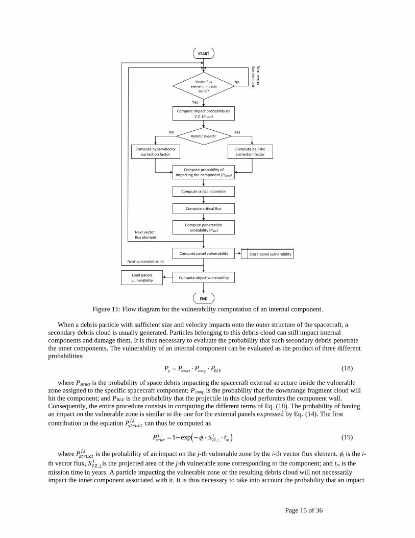
The analysis considered cylindrical and spherical tanks with varying thickness, material, and number of vessels.

The possible tank configurations ranges from one to six vessels and are positioned in a simplified fashion, as shown

in Figure 15. The circles represent the positions of the centre of each tank. The size and positioning of the tanks

follows the procedure of Section 4.3.3. In each configuration, the tanks have the same shape, i.e. they are all spheres

or cylinders.

of 36

Figure 15: Possible configuration for the positioning of the spacecraft tanks.

Different optimisation simulations were performed varying the range of the number of tanks, i.e. not just

performing the simulations with the maximum possible number of tanks.

An example of the Pareto front obtained with the optimisation is shown in Figure 16. The presented Pareto front

was obtained for a 2000 kg spacecraft in an 800 km altitude orbit, with a maximum number of tanks allowed equal to

three (configurations I, II, and III of Figure 15). The x-axis represents the survivability index, i.e. the Probability of

No-Penetration, and the y-axis represents the demisability index, i.e. the Liquid Mass Fraction. Both indices are

expressed in terms of percentage. It is possible to observe the general trend of the Pareto front, with the aluminium

solutions in the upper part (red solutions), representing the solutions with higher demisability but also a higher

vulnerability to debris impacts. The stainless steel solutions (blue solutions) are instead on the right part of the graph,

corresponding to solutions with higher survivability but lower demisability. No titanium solutions are present. This is

a common result for all the simulations performed, due to the extremely low demisability of titanium and its impact

resistance comparable to stainless steel.

of 36

Figure 16: Pareto front for a 2000 kg spacecraft and 10-year mission with a maximum allowed number of tanks equal

to three.

A gap is also observable between the aluminium and the stainless steel solutions. This is caused by the

considerable difference between the demisability of the two materials. In fact, two solutions with a slightly different

survivability coming from the different combination of material and thickness can have a remarkable difference in

the demisability because of the high influence of material properties on the demisability. All the solutions obtained

by the optimiser represent configurations with cylindrical tanks. In general, no solutions with spherical tanks were

obtained for the conditions used in this study. Another interesting consideration is the influence of the number of

tanks in the configuration. As it is possible to observe, in this case, all three configurations are viable solutions after

the optimisation. Configurations with lower amount of tanks have higher survivability and the lower demisability.

This is because the smaller the number of tanks in which to split the propellant, the bigger the tanks are and thus the

less demisable they are. However, they also have a lower external surface, which in turn means a higher

survivability. On the other hand, configurations with a higher number of tanks have smaller and more demisable

tanks but a higher external surface. They are also positioned closer to the external walls making them more

vulnerable to the debris impacts.

Figure 17 and Figure 18 represent two further examples of Pareto fronts for the previously introduced mission

scenario. In these cases, the maximum allowed number of tanks was respectively four and six. As it is possible to

observe in Figure 17 the only solutions resulting from the optimisation are those corresponding to Configuration IV,

with four tanks. Figure 18 has more variety of solutions with configurations comprising four, five, and six tanks.

However, there is a clear predominance of solutions with six tanks. In general, in all the optimisations performed, for

the different classes and mission scenarios, this trend was repeated.


to four.

The majority of the solutions were represented by the maximum allowed number of tanks. Despite the fact that a

higher number of tanks is also more exposed to debris impact, it is possible for the optimiser to find solutions with a

higher thickness to compensate for this while still maintaining a higher demisability than a solution with a lower

number of tanks. When this is no longer the case within the specified ranges of the optimisation, solutions with a

lower number of tanks become better. This behaviour is strictly correlated with how the demisability index is defined

(see Eq. (45) where the proportion of mass demised is considered. This is a reasonable choice for a demisability

index. In fact, while it is true that even a partially melted object reaches the ground and contributes to the casualty

risk, the uncertainty in re-entry simulations [52, 53] make the LMF index a good indication of how likely the

considered object will demise. It is in fact important to remember that the presented methodology involves a

preliminary assessment of many configurations. A further, more refined, analysis of the most promising

configurations can then be carried out to verify their quality. Another observable trend within Figure 16, Figure 17,

and Figure 18 is the reduction of the demisability gap between the aluminium alloy and the stainless steel solutions.

As the number of tanks increases, the maximum demisability of the stainless steel solutions also increases, closing

of 36

the gap with the aluminium alloy solutions. This indicates that to have demisable solutions for tanks made of

stainless steel, it is necessary to increase the number of vessels used, as only smaller tanks will be demisable.


to six.

As introduced in the previous paragraphs, the mission characteristics have also been taken into account. In

particular, the size of the spacecraft in terms of mass and external dimension (see Table 7), and the mission lifetime.

These aspects influenced the optimisation results, changing the shape and the features of the Pareto fronts. For

example, the minimum value of the PNP index corresponds to the configuration with the best demisability but also

the worst survivability. Such information gives an idea of how much an improved demisability can compromise the

survivability of a spacecraft, and as a function of the mission scenario. In Figure 19 it is possible to observe the

variation of the minimum survivability for each optimisation simulation as a function of the mission class and

lifetime, and for four different tank configurations.

Figure 19: Minimum survivability of the solutions in the Pareto front as a function of the mission class and lifetime.

of 36

As expected, the higher the mission lifetime, the lower the value of the minimum survivability. The same

happens as we increase the mission class. In fact, bigger spacecraft have a bigger probability of being hit by space

debris. The figure shows that for smaller spacecraft with limited lifetimes an enhanced demisability may not

compromise their survivability, giving the design team the possibility to push to more extreme solutions favouring

the demise. On the other hand, more massive and longer mission may need a more refined study because very

demisable solutions may compromise the reliability of the mission with respect to debris impacts. The difference is

in fact in the order of 2.5%, which is not negligible. In fact, the penetration probability of complete spacecraft

configurations is usually in the order of few percentage points (1-5%) [54]. Therefore, having the survivability of just

one component hampered by 1% or 2% would have a big relative impact on the overall survivability of a spacecraft.

It is true that this is a simplified simulation and many things can be changed in a spacecraft configuration to make it

less vulnerable, for instance the outer shielding. However, this study gives a first order evaluation of what the effects

can be when the survivability and the demisability are considered at the same time.

Another feature of the Pareto front that is heavily influenced by the simulation class and mission duration is the

demisability gap that is present between the aluminium solution with the smallest demisability and the steel solution

with the highest demisability. This gap provides an indication of how difficult it is for steel solutions to reach a

comparable demisability level with respect to aluminium solutions. Figure 20 shows a representation of the trend

relating to this demisability gap. As it is possible to observe, the higher the number of tanks in the configuration, the

smaller the gap for every type of mission scenario.

Figure 20: Demisability gap between the solutions in the Pareto front as a function of the mission class and lifetime.

There is a considerable gap between the solution with one tank and the other solutions with multiple tanks. It is

also possible to observe that the configurations with three and four tanks are very close and produce similar results. It

is also evident that the mission size is much more influential than the mission lifetime for this specific characteristic.

Bigger missions have larger tanks, which are of course more difficult to demise. This has a bigger impact on

solutions with less demisable materials such as the stainless steel.

5.1 Optimisation indices discussion

The optimisation framework presented in the previous paragraphs was aimed at demonstrating the

interdependence of the demisability and the survivability requirements when it comes to the design of spacecraft

components and configurations. To do so, a simplified spacecraft design with a single type of internal component

of 36

(i.e. tanks) was selected. In order to relate the results obtained to actual mission scenarios, the propellant mass and,

as a consequence, the dimensions of the tanks was related to the delta-V budget of sun-synchronous missions (see

Section 0). The optimiser is free to look for solutions inside the search space defined in Table 5. No other constraints

were added to the optimisation problem. For example, there was no limit on the overall mass of the configuration or

complexity of the propulsion regulation system, and no check if the tanks were sufficiently strong to withstand the

common storage pressures, etc. It is thus interesting to compare the obtained solutions against some of these

characteristics. In Figure 21 a Pareto front is presented for a 2000 kg class mission with seven years of mission

lifetime and a maximum allowed numbers of tanks equal to three.

To the plot is associated the variation of the ratio between the tank configuration mass and the propellant mass

for each solution. As it is possible to observe, the mass tends to increase as the solutions move from the more

vulnerable and more demisable solutions to the more survivable and less demisable solutions. However, there are

solutions corresponding to configurations with a number of tanks lower than the maximum allowed, which have a

lower mass thus producing the valleys in the graph. Usually spacecraft propellant tanks have a mass raging between

10% and 20% of the propellant mass stored, and they can reach 50% for high storage pressures [35]. In Figure 21,

such solutions are highlighted in red in both plots. It is possible to observe that only aluminium alloy solutions

belong to the typical mass range for the specific mission. However, some stainless steel solutions are not too far

away from the considered range and, considering this is a preliminary design analysis, some of them could be

included during the later stages of the mission design process. In addition, it is possible to observe that all three kinds

of configuration (one, two, and three tanks) are present in the typical range, giving a wider variety of options to the

design team.

Figure 21: Pareto front for a 2000 kg, 7 years mission with maximum 3 tanks, with variation of the ratio between the

tank configuration and the propellant mass. Highlighted (red lines and symbols) the solutions inside the typical range

for actual missions.

Another important aspect to look at is the actual feasibility of the solutions, i.e. whether the tanks are actually

able to sustain the normal operating pressures. Typically, a propellant tank has a storage pressure between 2 and 4

MPa. For cylindrical tanks, which constitute the solutions obtained in the Pareto front, the stress on the tanks’ walls

can be computed as follows:

t

w

t

pr

t = (51)

of 36

where σw is the stress on the walls of the tank, and p is the storage pressure. The computed tension has to be lower

than the ultimate tensile strength of the material of the tank. This in turn imposes a limit on the maximum pressure

that a tank with a certain radius, thickness and material can withstand, which is [35]:

max

u t

t

tp

r SF

=

(52)

where σu is the ultimate tensile strength of the material, and SF is a safety factor assumed equal to 1.5 for the current

study. In Figure 22 the same Pareto front as before is presented. In this case the second plot represent the maximum

sustainable storage pressure of the solutions belonging to the Pareto front and computed with Eq. (52). Even in this

case, the solutions within the common limits (2-4 MPa) have been highlighted in red. As it is possible to observe,

both aluminium alloy and stainless steel solutions belong to the highlighted range. Obviously, all the stainless steel

solutions would be viable as they can resist a storage pressure higher than the 4 MPa limit. The aluminium alloy

solutions outside the range, on the other hand, would be too thin to withstand the operating pressures normally used.

Figure 22: Pareto front for a 2000 kg, 7 years mission with maximum 3 tanks, with variation of the maximum storage

pressure. Highlighted (red lines and symbols) the solutions inside the typical range of propellant storage pressures.

Finally, we can consider a more casualty risk related parameter that is the on-ground impact energy. As was

mentioned, the demisability index adopted in this study has some limitations because it only considers the percentage

of demised mass. However, it is also important to know the mass that actually lands on the surface, and even more

important is to know the impact energy of the re-entering object. In fact, the NASA standard [3] states that a

surviving object does not pose a risk for people on the ground if it has an impact energy below 15 J. This means the

impact energy is an important parameter when considering the demisability of spacecraft components. In Figure 23,

the impact energy of each solution in the Pareto front is represented.

of 36

Figure 23: Pareto front for a 2000 kg, 7 years mission with maximum 3 tanks, with variation of the final energy of

the re-entering object. Highlighted (red lines and symbols) the solutions below the 15 J threshold.

There are many solutions below the 15-joule threshold; however, all of them are made of aluminium alloy. Stainless

steel solutions reaching the surface are usually too heavy to have such a low impact energy. However, the 15-joule

limit is quite specific and, given the uncertainty intrinsic to re-entry simulations, it probably should not constitute a

hard boundary to the validity of a solution, especially during a preliminary design phase. It is evident from this analysis

of the solutions obtained from the optimisation that some improvements need to be introduced to the formulation of

the optimisation itself. In fact, it is more efficient and more useful to obtain solutions that already take into account

mission related constraints such as the overall mass of the system or its strength, as well as the casualty risk

requirements. This can be obtained through a different definition of the fitness functions. For example, by changing

the demisability index so that it includes a way to take into account the impact energy of the re-entering components.

Moreover, a set of constraints can be introduced during the optimisation to take into account the limitations such as

the maximum allowed storage pressure.

5.2 Multi-objective optimisation discussion

As introduced at the beginning of Section 4, the strategy proposed for the development of the multi-objective

optimisation framework described in the paper is the one of evolutionary algorithms. The selection of these types of

algorithms has been based on the characteristics they present with respect to the problem in exam. Given their

population-based approach, genetic algorithms are well suited to solve multi-objective optimisation problems such as

the one we are considering [55]. In addition, they allow the simultaneous search of different regions of the search

space, making it possible to find a very diverse set of solutions for difficult problems were the search space is

discontinuous. This is particularly true for the type of problem presented in the paper, where the search space is

composed of both continuous and discrete variables. Moreover, the aim of the optimisation framework under

development is the exploration of the large design space of preliminary spacecraft configuration in order to be able to

find viable solutions that can be studied more in depth in later stages of the mission design process. This is exactly one

of the situations where evolutionary algorithms excel. However, given their stochastic nature, evolutionary algorithms

can only find an approximation of the Pareto front and not the actual front. Nonetheless, for the purpose of the

developed framework, the aim is to find a set of preliminary solutions and the approximate nature of evolutionary

algorithms can thus be accepted.

of 36

5.2.1 Models and optimisation computational costs

When looking at optimisation it is also important to look at the computational cost of the simulation. The developed

code is entirely written in Python and the simulations for the article have been performed on an 8-core Intel i7 at 3.4

GHz PC with 16 GB of RAM. A summary of the average simulation times for a single simulation of both the

demisability and survivability models are shown in Table 8, together with the average time for an optimisation

simulation. The single simulations are not parallelised, whereas the optimisation cost is for a simulation parallelised

on the 8 cores of the PC.

Table 8: Computational cost of the demisability model, survivability model, and optimisation simulation. The values

in the table are the average over the different simulations performed in the study.

Demisability model Survivability model

Avg. single simulation time (s) 2.46 1.6

Avg. optimisation execution time (s) 3557.2

The simulation times for the models are not constant; they depend on the characteristics of the spacecraft

configuration. For example, it is possible to observe from Figure 24 that the demisability model cost is influenced by

both the thickness and size (number of vessels) of the tanks. This is a consequence of the different ballistic coefficients

resulting for the different tanks configurations, which influence the shape of the trajectory. The survivability model

(Figure 25) instead is more influenced by the number of vessels, as for each vessel the penetration probability as to be

computed separately.

Figure 24: Demisability model computational cost for

cylindrical aluminium alloy tanks as a function of the

thickness and number of vessels.

Figure 25: Survivability model computational cost for

cylindrical aluminium alloy tanks as a function of the

thickness and number of vessels.

5.2.2 Indices behaviour

A further justification supporting the use of an evolutionary algorithm to explore the search space under the

requirements of the demisability and of the survivability is given by the behaviour of the two indices as a function of

the optimisation variables. An example of the discontinuous and nonlinear behaviour of the indices as a function of

the tank thickness and material type is given in Figure 26 and Figure 27. The example refers to a two vessels cylindrical

tank configuration. It is possible to observe how both indices have different values when changing the material,

especially the demisability index. In addition, even the behaviour of the indices with respect to the thickness is not

linear and can still have discontinuity. In the case of the demisability index, it follows an almost logarithmic trend. On

the other end, the demisability index shows a very different behaviour depending on the material. For the titanium

alloy a constant value of zero, for the stainless steel a dogleg curve with a maximum around 1.5 mm, and for the

aluminium alloy, an initial flat curve shows a discontinuity around 3.6 mm.

of 36

Figure 26: Demisability index trends as a function of the

tank thickness and material for a two vessels assembly

with cylindrical tanks.

Figure 27: Survivability index trends as a function of the

tank thickness and material for a two vessels assembly

with cylindrical tanks.

5.2.3 Future developments of the optimisation framework

The optimisation framework has been applied to a simplified example, which was selected to illustrate the

capabilities of the framework. It is meant to demonstrate the applicability and the efficacy of multi-objective

optimisation using genetic algorithms to the wide exploration of preliminary spacecraft design solutions under the

requirements of the demisability and of the survivability. The introduced optimisation framework is being developed

in order to be able to analyse more complete satellite configurations, which include several components, of different

types (e.g. tanks, reaction wheels, batteries, payloads, external panels, etc.). Not only the characteristics of the single

components such as dimensions, thickness, material, and shape will be optimisable; also, their position inside the

spacecraft and their possible attachment to the panels of the main structure will be considered. It will also be possible

to handle component specific constraints and associate them with mission specific characteristics. For example, the

minimum thickness required by a tank with given shape, material, size, and given the propellant required by the mission

and the maximum specified storage pressure; or the minimum radius of a reaction wheel given its material, rotation

speed, and mission required angular momentum.

Despite the dimensionality of the presented test case is low with only 4 optimisation variables, with the

development of the framework, the complexity of the optimisation problem will quickly increase. For example, if we

consider 4 optimisable components similar to the one used in the test case (i.e. 4 variables, 3 discrete and 1 continuous)

and we add the possibility to optimise the position (3 continuous variables for each component), we pass from 4 to 28

variables (12 discrete and 16 continuous). We decided to use genetic algorithm with in mind the necessity to explore

such large search spaces [56], characterised by both continuous and discrete variables. The example presented is used

to demonstrate the applicability of the framework and shows the competing nature of the demisability and survivability

requirements.

6 Conclusions

An optimisation framework that analyses preliminary spacecraft design options against the requirements posed

by the demisability and the survivability has been proposed and described. The framework has then been applied to a

simplified test case in order to demonstrate its characteristics and applicability, as well as the influence of the

demisability and survivability requirements on the design choices. The test cases considered spacecraft in sun-

synchronous missions and a specific type of internal component to optimise (tank assemblies). Two fitness functions

describing the demisability and the survivability have been presented, and different tank configurations have been

analysed as a function of their material, geometry, and configuration. The optimiser is able to provide a wide range

of solutions for different types of mission scenarios. Some trends could be observed in the output of the optimisation

for the different scenarios as a function of the mission class, lifetime and of the maximum allowed number of tanks

in the configuration. For example, no titanium solutions were observed, nor were configurations with spherical tanks

obtained.

A more in depth analysis of the solutions obtained showed that only a subset of the solutions belonged to typical

configurations with respect to the mass and strength of the configuration. Moreover, only certain solutions in the

Pareto front could satisfy the casualty risk criterion of the 15-joule threshold. This means that a further effort needs

to be made in the definition of the optimisation problem through a more tailored definition of the demisability and

survivability indices and through the application of constraints during the optimisation. Considering these additional

of 36

properties may lead to a different set of solutions. For example, spherical tanks may be present because of their

capability to withstand higher storage pressures with respect to cylindrical tanks with the same volume.

The developed optimisation framework has been introduced and tested on a simplified example. Future

development of the framework will allow the optimisation of more complex spacecraft configurations, with many

types of components (tanks, reaction wheels, batteries, etc.). In addition, the definition of mission and component

specific constraints will be possible.

Acknowledgments

Part of this work was funded by EPSRC DTP/CDT through the grant EP/K503150/1. All data supporting this

study are openly available from the University of Southampton repository at https://doi.org/10.5258/SOTON/D0036.

References

[1] B. O'Connor 2008. Handbook for Limiting Orbital Debris. NASA Handbook 8719.14. National Aeronautics

and Space Administration, Washington, DC.

[2] F. Schäfer, M. Lambert, E. Christiansen et al. The inter-agency space debris coordination committee (IADC)

protection manual. 4th European Conference on Space Debris, 2005.

[3] NASA 2012. Process for Limiting Orbital Debris. Washington, DC USA.

[4] European Space Agency 2008. Requirements on Space Debris Mitigation for ESA Projects.

[5] R. L. Kelley. Using the Design for Demise Philosophy to Reduce Casualty Risk Due to Reentering Spacecraft.

63rd International Astronautical Congress, 1-5 October 2012 Naples, Italy.

[6] P. M. Waswa, and J. A. Hoffman 2012. Illustrative NASA Low Earth Orbit spacecraft subsystems design-

for-demise trade-offs, analyses and limitations. International Journal of Design Engineering, 5, 21-40.

[7] P. M. B. Waswa, M. Elliot, and J. A. Hoffman 2013. Spacecraft Design-for-Demise implementation strategy

& decision-making methodology for low earth orbit missions. Advances in Space Research, 51, 1627-1637.

[8] E. Christiansen 2009. Handbook for Designing MMOD Protection. Huston, Texas USA.

[9] R. Putzar, and F. Schäfer, Vulnerability of spacecraft equipment to space debris and meteoroids impacts,

Final Report, vol. 1, European Space Agency, 2006.

[10] L. Grassi, F. Tiboldo, R. Destefanis et al. 2014. Satellite vulnerability to space debris – an improved 3D risk

assessment methodology. Acta Astronautica, 99, 283-291.

[11] M. Trisolini, H. G. Lewis, and C. Colombo. Survivability and Demise Criteria for Sustainable Spacecraft

Design. 66th International Astronautical Conference, 2015 Jerusalem.

[12] H. Schaub, L. E. Jasper, P. V. Anderson et al. 2015. Cost and risk assessment for spacecraft operation

decisions caused by the space debris environment. Acta Astronautica, 113, 66-79.

[13] M. Trisolini, H. G. Lewis, and C. Colombo. Demise and Survivability Criteria for Spacecraft Design

Optimisation. International Association for the Avancement of Space Safety Conference, 18-20 May 2016

Melbourne, Florida.

[14] M. Trisolini, H. G. Lewis, and C. Colombo. Demisability and survivability multi-objective optimisation for

preliminary spacecraft design 68th International Astronautical Congress, 25-30 September 2017 Adelaide,

Australia.

[15] M. Trisolini, H. G. Lewis, and C. Colombo 2016. Demise and survivability criteria for spacecraft design

optimization. Journal of Space Safety Engineering, 3, 83-93.

[16] NASA. 2009. ORSAT [Online]. NASA Orbital Debris Program Office. Available:

http://orbitaldebris.jsc.nasa.gov/reentry/orsat.html [Accessed July 14 2015].

[17] NASA. 2015. Debris Assessment Software [Online]. NASA Orbital Debris Program Office. Available:

http://orbitaldebris.jsc.nasa.gov/mitigate/das.html [Accessed July 14 2015].

[18] T. Lips, and B. Fritsche 2005. A comparison of commonly used re-entry analysis tools. Acta Astronautica,

57, 312-323.

[19] E. Minisci. 2015. Space Debris and Asteroids (Re)Entry Analysis Methods and Tools [Online]. Glasgow, UK:

University of Strathclyde. Available: https://www.mat.uniroma2.it/Astro/slides/SSTS/SSTS-Minisci.pdf.

[20] J. Gelhaus, C. Kebschull, V. Braun et al., DRAMA Final Report - Upgrade of ESA's Space Debris Mitigation

Analysis Tool Suite, European Space Agency, 2014.

[21] C. Martin, J. Cheeses, N. Sanchez-Ortiz et al. 2005. Introducing the ESA DRAMA tool. Science and

Technology Series, 110, 219-233.

https://doi.org/10.5258/SOTON/D0036

http://orbitaldebris.jsc.nasa.gov/reentry/orsat.html

http://orbitaldebris.jsc.nasa.gov/mitigate/das.html

https://www.mat.uniroma2.it/Astro/slides/SSTS/SSTS-Minisci.pdf

of 36

[22] G. Koppenwallner, B. Fritsche, T. Lips et al. Scarab-a Multi-Disciplinary Code for Destruction Analysis of

Space-Craft during Re-Entry. Fifth European Symposium on Aerothermodynamics for Space Vehicles, 2005.

281.

[23] NASA 1976. U.S. Standard Atmosphere 1976. Washington, D.C.

[24] A. Tewari 2007. Atmospheric and Space Flight Dynamics: Modeling and Simulation with MATLAB® and

Simulink®, Birkhäuser.

[25] R. D. Klett, Drag Coefficients and Heating Ratios for Right Circular Cylinder in Free-Molecular and

Continuum Flow from Mach 10 to 30, Technical Report SC-RR-64-2141, Sandia Report, SC-RR-64-2141,

Albuquerque, 1964.

[26] W. P. Hallman, and D. M. Moody, Trajectory Reconstruction and Heating Analysis of Columbia Composite

Debris Pieces, The Aerospace Corporation, Cambridge, MA, USA, 2005.

[27] T. M. Owens. 2014. Aero-Thermal Demise of Reentry Debris: A Computational Model. Master of Science,

Florida Insititute of Technology.

[28] J. Beck. May 5 2015. RE: Personal Communication.

[29] MatWeb LLC. 2015. MatWeb - Material Property Data [Online]. Available: http://www.matweb.com/

[Accessed February 2015].

[30] S. Flegel 2011. MASTER-2009 Software User Manual. Institute of Aerospace Systems (ILR).

[31] W. P. Schonberg 2001. Characterizing secondary debris impact ejecta. International Journal of Impact

Engineering, 26, 713-724.

[32] D. Depczuk, and W. Schonberg 2003. Characterizing debris clouds created in oblique orbital debris particle

impact. Journal of Aerospace Engineering, 16, 177-190.

[33] N. Welty, M. Rudolph, F. Schäfer et al. 2013. Computational methodology to predict satellite system-level

effects from impacts of untrackable space debris. Acta Astronautica, 88, 35-43.

[34] S. Ryan, and E. Christiansen 2011. A ballistic limit analysis programme for shielding against micrometeoroids

and orbital debris. Acta Astronautica, 69, 245-257.

[35] J. R. Wertz, and W. J. Larson 1999. Space Mission Analysis and Design, Springer Netherlands.

[36] S. Platnick. 2016. NASA's Earth Observing System [Online]. National Aeronautics and Space Administration.

Available: http://eospso.nasa.gov/mission-category/3 [Accessed January 2016].

[37] Airbus Safran Launchers GmbH. 2003. Space Propulsion [Online]. Bremen, Germany. Available:

http://www.space-propulsion.com/index.html [Accessed July 2016].

[38] European Space Agency. 2012. Metop - meteorological missions [Online]. European Space Agency.

Available:

http://www.esa.int/Our_Activities/Observing_the_Earth/The_Living_Planet_Programme/Meteorological_m

issions/MetOp/Overview14 [Accessed January 2016].

[39] European Space Agency. 2016. CryoSat-2 (Earth Explorer Opportunity Mission-2) [Online]. eoPortal

Directory. Available: https://eoportal.org/web/eoportal/satellite-missions/c-missions/cryosat-2 [Accessed

July 2016].

[40] K. Deb 2001. Multi-objective optimization using evolutionary algorithms, John Wiley & Sons.

[41] K. Deb, A. Pratap, S. Agarwal et al. 2002. A fast and elitist multiobjective genetic algorithm: NSGA-II.

Evolutionary Computation, IEEE Transactions on, 6, 182-197.

[42] F. A. Fortin, F. M. De Rainville, M. A. Gardner et al. 2012. DEAP: Evolutionary Algorithms Made Easy.

Journal of Machine Learning Research, 13, 2171-2175.

[43] K. Deb, and R. B. Agrawal 1995. Simulated binary crossover for continuous search space. Complex systems,

9, 115-148.

[44] K. Deb, and D. Deb 2014. Analysing mutation schemes for real-parameter genetic algorithms. International

Journal of Artificial Intelligence and Soft Computing, 4, 1-28.

[45] J. N. Opiela, E. Hillary, D. O. Whitlock et al., Debris Assessment Software Version 2.0 - User's Guide, Lyndon

B. Johnson Space Center, Huston, Texas, 2012.

[46] ASM Aerospace Specification Metals Inc. 2016. ASM Aerospace Specification Metals [Online]. Pompano

Beach, Florida. Available: http://www.aerospacemetals.com/contact-aerospace-metals.html [Accessed July

2016].

[47] H. Stokes, C. Cougnet, J. Gelhaus et al., “A Detailed Impact Risk Assessment of Two Low Earth Orbiting

Satellites,” in International Astronautical Congress, Naples, Italy, 2012.

[48] W. Kuiper, G. Drolshagen, and R. Noomen 2010. Micro-meteoroids and space debris impact risk assessment

for the ConeXpress satellite using ESABASE2/Debris. Advances in Space Research, 45, 683-689.

http://www.matweb.com/

http://eospso.nasa.gov/mission-category/3

http://www.space-propulsion.com/index.html

http://www.esa.int/Our_Activities/Observing_the_Earth/The_Living_Planet_Programme/Meteorological_missions/MetOp/Overview14

http://www.esa.int/Our_Activities/Observing_the_Earth/The_Living_Planet_Programme/Meteorological_missions/MetOp/Overview14

https://eoportal.org/web/eoportal/satellite-missions/c-missions/cryosat-2

http://www.aerospacemetals.com/contact-aerospace-metals.html

of 36

[49] H.-G. Reimerdes, and W. Wohlers. Optimization of micrometeoroid and space debris protection systems.

Third European Conference on Space Debris, 2001 Darmstadt, Germany. 655-660.

[50] J. Beck, J. Merrifield, I. Holbrough et al. 2015. Application of the SAM Destructive Re-Entry Code to the

Spacecraft Demise Integration Test Cases. 8th European Symposium on Aerothermodynamics of Space

Vehicles, 2-6 March 2015 Lisbon.

[51] B. Fritsche, T. Lips, and G. Koppenwallner 2007. Analytical and numerical re-entry analysis of simple-shaped

objects. Acta Astronautica, 60, 737-751.

[52] J. Merrifield, J. Beck, G. Markelov et al. Aerothermal Heating Methodology in the Spacecraft Aerothermal

Model (SAM). 7th IAASS Conference, 2014.

[53] J. Merrifield, J. Beck, G. Markelov et al. Simplified Aerothermal Models for Destructive Entry Analysis. 8th

European Symposium and Aerothermodynamics for Space Vehicles, 2015.

[54] K. Bunte, R. Destefanis, and G. Drolshagen. Spacecraft Shielding Layout and Optimisation Using

ESABASE2/Debris. 5th European Conference on Space Debris, 30 March - 2 April 2009 ESOC, Darmstadt,

Germany.

[55] A. Konak, D. W. Coit, and A. E. Smith 2006. Multi-objective optimization using genetic algorithms: A

tutorial. Reliability Engineering & System Safety, 91, 992-1007.

[56] P. H. Stokes, and G. G. Swinerd 2004. The implementation of cost effective debris protection in unmanned

spacecraft. Advances in Space Research, 34, 1090-1096.

spacecraft design optimisation for demise and survivability

Documents