The University of Manchester Research

Spacecraft drag modelling

DOI:10.1016/j.paerosci.2013.09.001

Document VersionAccepted author manuscript

Link to publication record in Manchester Research Explorer

Citation for published version (APA):Mostaza Prieto, D., Graziano, B. P., & Roberts, P. C. E. (2014). Spacecraft drag modelling. Progress in AerospaceSciences, 64, 56-65. https://doi.org/10.1016/j.paerosci.2013.09.001

Published in:Progress in Aerospace Sciences

Citing this paperPlease note that where the full-text provided on Manchester Research Explorer is the Author Accepted Manuscriptor Proof version this may differ from the final Published version. If citing, it is advised that you check and use thepublisher's definitive version.

General rightsCopyright and moral rights for the publications made accessible in the Research Explorer are retained by theauthors and/or other copyright owners and it is a condition of accessing publications that users recognise andabide by the legal requirements associated with these rights.

Takedown policyIf you believe that this document breaches copyright please refer to the University of Manchester’s TakedownProcedures [http://man.ac.uk/04Y6Bo] or contact uml.scholarlycommunications@manchester.ac.uk providingrelevant details, so we can investigate your claim.

Download date:16. Mar. 2020

Spacecraft Drag Modelling

David Mostaza Prieto; Benjamin P. Graziano; Peter C. E. Roberts

Space Research Centre, Cranfield University

Abstract

This paper reviews currently available methods to calculate drag coefficients

of spacecraft traveling in low Earth orbits (LEO). Aerodynamic analysis of satel-

lites is necessary to predict the drag force perturbation to their orbital trajectory,

which for LEO orbits is the second in magnitude after the gravitational distur-

bance due to the Earth’s oblateness. Historically, accurate determination of the

spacecraft drag coefficient (CD) was rarely required. This fact was justified by

the low fidelity of upper atmospheric models together with the lack of experi-

mental validation of the theory. Therefore, the calculation effort was a priori

not justified. However, advances on the field, such as new atmospheric models

of improved precision, have allowed for a better characterization of the drag

force. They have also addressed the importance of using physically consistent

drag coefficients when performing aerodynamic calculations to improve analysis

and validate theories. We review the most common approaches to predict these

coefficients.

Keywords: Spacecraft drag; Free Molecular Flow; Rarefied Aerodynamics

1. Introduction

The study of the upper atmosphere is a key issue on the determination

and prediction of spacecraft trajectories. The drag force resulting from the

interchange of momentum between the upper atmosphere and spacecraft reduces

the orbital energy. The result is a change of the eccentricity towards a more

circular orbit, together with a reduction of the semi major axis until the eventual

re-entry of the spacecraft.

Preprint submitted to Progress in Aerospace Sciences September 7, 2016

Although it is known that in LEO orbits the drag force is the biggest source

of perturbation after the J2 coefficient of the gravitational potential function

of the Earth, an accurate prediction and determination of its magnitude is still

challenging. A common approach to calculate the drag acceleration experienced

by a body is:

adrag =1

2ρV 2CD

S

m(1)

Where ρ represents the atmospheric density, V is the relative velocity of the

vehicle with respect to the atmosphere, CD is the drag coefficient, S is the

reference surface area and m the mass of the body. A good estimation of adrag

is often difficult to obtain. This is due to the large uncertainties associated with

three of the above parameters: density, drag coefficient and velocity of the body

with respect to the atmosphere:

• Neutral density of the upper atmosphere, ρ, is the major source of error

in the determination of the drag force. The atmosphere is a moving mass

of air, and its density varies with time, altitude and geographical loca-

tion. The main driver of these changes at satellite altitudes is the varying

extreme ultraviolet (EUV) radiation from the sun since temperature and

hence density are affected by the amount of energy absorbed in the upper

atmosphere. The result is a long term trend related to the 11 years solar

cycle together with more transient and localised effects due to diurnal, sea-

sonal, longitudinal, and latitudinal variations in atmospheric conditions.

Also geomagnetic fluctuations caused by solar storms, which take place

more frequently during periods of peak solar activity, have been shown to

increase thermospheric density several factors [14]. Historically few data

have been available and, as a consequence, upper atmosphere neutral den-

sity models are not precise. Its current accuracy is lies between 10% and

15% in mean activity conditions [38], however it can go up to 100% for

short term and local variations [1]. The early upper atmospheric models

2

were derived from orbit tracking of different satellites, with the density

computed assuming a constant CD and neglecting winds [22]. For a good

review of available atmospheric models and atmospheric modelling issues

refer to [11, 16, 17, 22, 38].

• Relative velocity, V . A common assumption to calculate relative velocity

is to consider that the atmosphere rotates with the Earth. The presence of

wind adds uncertainty to the problem. In-track winds can either increase

or decrease the drag force depending on the blowing direction. It has been

demonstrated that strong winds of several hundred meters per second can

take place in the upper atmosphere (specially at high latitudes) and very

little prediction capability is available to date [12, 20].

• Drag coefficient, CD. It has been a common practice to assume a constant

CD equal to 2.2 for low earth orbit flying satellites. Due to the lack of

precision of existing atmospheric density models, any modelling effort to

refine the drag coefficient was normally considered of little advantage,

since it does not compensate for the imprecise density model. Nowadays,

it is widely accepted that the drag coefficient is not constant and can

present very different values depending on the spacecraft shape and the

atmospheric temperature and composition at the flying altitude. Note that

atmospheric density models obtained from satellite observations, directly

incorporate any error on the drag coefficient as density biases.

Despite the described difficulties, in recent times there has been an increased

interest in spacecraft drag modelling. We have entered the 21st century inside

a Golden Age of Satellite Drag [17] mainly due to new dedicated space missions

together with more and more available data and a better understanding of the

solar phenomena. Many research groups have become interested in the topic

in the last few years, and even more interest is foreseen in the future. Any

improvement on the knowledge of this disturbance will directly impact the ac-

curacy of mission analysis and orbital predictions. This will result, for instance,

3

in better orbit determination and tracking of space objects (allowing for ex-

ample optimum and precise collision avoidance manoeuvres), in more accurate

determination of re-entry windows and debris footprints or in finer optimisation

of fuel budgets. A comprehensive aerodynamic characterization of the space-

craft is also needed to study new mission concepts in which the aerodynamic

force plays an active roll, such as drag compensation, sub-orbital flights, drag

optimization, or trajectory and attitude control by means of aerodynamic forces

and torques.

This paper is focused on the numerical and analytical calculation of CD (and

associated aerodynamic coefficients) for bodies traveling in low Earth orbit.

2. Characterising the environment

The neutral atmospheric region of interest in the study of satellite aerody-

namics is the thermosphere, a high-altitude layer that exist above around 85

km. The thermosphere absorbs the EUV energy from the Sun resulting in a

temperature profile increasing rapidly with altitude at its lower part (below

around 200 km). In its upper region, the temperature increase reaches a lim-

iting value (exospheric temperature) and remains constant with altitude due

to the the infrequency of intermolecular collisions that occur as a result of the

very low density. The temperature and neutral density vary with the amount

of energy received by the the thermosphere. The main energy sources affecting

its structure are the the solar flux and the geomagnetic activity.

The biggest variation in solar flux is due to the 11 years solar cycle, tem-

perature and neutral density tend to follow the same trend. Variations in mean

density profiles for low, mean, and high levels of solar and geomagnetic activi-

ties, as defined by [1], are illustrated in Fig. 1. Density variations increase with

altitude; notice that for an altitude of 600 km, the atmospheric density varies

by up to almost two orders of magnitude. This density increase during high

solar activity periods is the dominant factor affecting spacecraft aerodynamic

performance [41]. One well-known consequence of this variation is that during

4

100 200 300 400 500 60010

−14

10−13

10−12

10−11

10−10

10−9

10−8

10−7

10−6

Altitude [km]

ρ [

kg

/m3]

Mean

High

Low

Figure 1: Variation of the mean atmospheric density with altitude for low, moderate and high

solar and geomagnetic activities as defined by JB2006 model. Reproduced from [1]

these periods, satellites in low Earth orbit deorbit more quickly and have their

operational lifetimes reduced as a result.

Two indices are generally used to measure the solar radiation and geomag-

netic activity levels:

• F10.7 index for solar flux: It is a measure of the solar flux emitted at

a wavelength of 10.7 cm. Since the EUV radiation is absorbed in the

thermosphere it is difficult to obtain a measurement of the solar flux at

these wavelengths using instruments at the Earth’s surface. It has been

found that the F10.7 index presents a good correlation with solar activity

[36]. Currently it is used as a proxy for EUV radiation in atmospheric

models.

• Ap index for geomagnetic activity: This index is a measure of the general

level of geomagnetic activity on the Earth for a given day. It is obtained

from measurements of the magnetic field variations made at different lo-

5

100 200 300 400 500 600 700 800 90010

4

106

108

1010

1012

1014

1016

1018

Altitude [km]

num

ber d

ensit

y [m

−3]

HeON2O2

ArHN

Figure 2: Variation of the Earth’s atmospheric composition with altitude as defined by NRLM-

SISE00 model. Reproduced from [1]

cations. Geomagnetic storms are characterized by a sudden increase of

this index.

At the considered altitudes, the composition of the atmospheric gas mixture

varies with altitude, as illustrated in Fig. 2. Lighter molecules are faster, due to

acquiring the same energy as heavier molecules on average from collisions. The

faster molecules have a different scale height and are also lost to space more

easily. In addition to these variations, atmospheric composition with altitude

will fluctuate as the atmosphere expands and contracts under the influence of

the solar cycle or geomagnetic activity.

Several models to predict atmospheric characteristics at spacecraft altitudes

have been published since the 1960s. They provide values for neutral density

and temperature as a function of the spacecraft position, solar radiation and

geomagnetic activity. Two of the most modern models are briefly presented

6

here: the NRLMSISE00 and the JB2006.

• NRLMSISE00 [28]. This model provides temperature and gas species

number densities (for He,O,N2, O2, Ar,H and N) covering all the range

from sea level up to the exosphere. Inputs to the model are altitude,

latitude, longitude and the two indices F10.7 andAp. A component named

”anomalous oxygen” is introduced in the model for drag estimation. It

accounts for the contribution of non thermospheric species to the drag

at high altitudes, such as O+ and hot oxygen (energetic oxygen atoms

resulting from photochemical processes in the upper atmosphere [42]).

• JB2006 [6]. This models provides neutral density and temperature from

120 km to the exosphere. Input parameters are F10.7 and Ap, however,

it also incorporates new solar indices (S10 and Mg10) to obtain better

density variation correlations with UV radiation together with a model

of the semi annual density variation [4]. A further improvement in the

modeling and results is the JB2008 version [5].

According to the ECSS standard on Space environment [1], the NRLM-

SISE00 model shall be used for calculating neutral temperature, detailed com-

position and total density below 120 km, whereas the JB2006 model shall be

used for calculating the total density above 120 km. It is worth mentioning

that atmospheric models up to date only predict slow time variations and large

scales.

2.1. Free Molecular Flow

The highly rarefied atmosphere of low Earth orbit requires a different ap-

proach to aerodynamics than that employed in the continuum regime that exists

at aircraft flight altitudes. Due to the low density, the flow regime of low Earth

orbit spaceflight is commonly described as free molecular. This means that

the mean-free path (the mean distance between consecutive collisions, which

is illustrated in Fig. 3) is many times greater than the characteristic dimen-

sion of a body immersed in the flow. Therefore, collisions between molecules

7

Spacecraft Aerodynamics

18

Humanity’s influence on the upper atmosphere will benefit some spacecraft missions. For example, low Earth orbiting satellites will require fewer aerodynamic drag correction manoeuvres and have an increased lifespan.

Unfortunately, the anthropogenic effects on the upper atmosphere will also cause post-operational spacecraft debris to remain in orbit longer. Thus strengthening the case for all future low Earth orbit satellites to incorporate some means of eliminating their own debris threat over shorter timescales than today’s spacecraft.

2.2 Free Molecular Flow

The highly rarefied atmosphere of low Earth orbit requires a different approach to aerodynamics than that employed in the continuum regime that exists at aircraft flight altitudes and below. The following sections will define the regime of low Earth orbit spaceflight and then provide details of the various characteristics and mathematical parameters of the regime that are of interest to the spacecraft aerodynamicist.

2.2.1 Regime Definition

The flow regime of low Earth orbit spaceflight is commonly described as free molecular. This means that the mean-free path between atmospheric gas molecules (the mean distance between consecutive collisions), which is illustrated in Figure 2-8, is many times greater than the characteristic dimension of a body immersed in the flow. Therefore, collisions between molecules are extremely rare in the flow field around the body, such that the flow can be assumed collisionless.

Figure 2-8 - Molecular Mean Free Path (!!!!) A non-dimensional parameter known as a Knudsen number (Kn), given by

Equation 2-1, is commonly used to define low-density flow regimes. It indicates the

Figure 3: Molecular Mean Free Path (λ)

are extremely rare in the flow field around the body, such that the flow can

be assumed collisionless and it cannot be considered as a continuum medium

anymore. Instead it is particulate in nature.

To quantify the validity of the collisionless assumption a non-dimensional

parameter known as Knudsen number is used.

Kn =λ

lref(2)

The term lref is the characteristic dimension of the spacecraft and λ is the

mean free path. A high Kn indicates that the flow is particulate in nature

(i.e. free molecular) and that the collisionless Boltzmann equation should be

employed, a low Kn indicates that the flow is continuum in nature and should

be analysed using the Navier-Stokes equations. It is generally assumed in most

rarefied gas dynamics literature that the free molecular flow assumption is valid

for Kn ≥ 10 [25]. Fig. 4 shows the Knudsen number variation with altitude

and Fig. 5 illustrates how Knudsen number can be used to describe rarefied

flow regimes.

Another important parameter in free molecular flow is the molecular speed

8

100 200 300 400 500 60010

1

102

103

104

105

106

107

Altitude [km]

Kn

ud

se

n

Mean

High

Low

Figure 4: Knudsen number variation with altitude for low, moderate and high solar and

geomagnetic activities using NRLMSISE-00, and a characteristic dimension of 1 m

Spacecraft Aerodynamics

19

degree of rarefaction and hence the difference between continuum and non-continuum flow.

reflKn != 2-1

The term lref is the characteristic dimension of the spacecraft and the mean-free path ! can be approximated in rarefied flow by the semi-empirical Equation 2-2 [18].

pdkT

avg22"

! = 2-2

The term k is the Boltzmann constant (1.3807 ! 10-23 J K-1), T is the kinetic gas temperature (in Kelvin), davg is the mean collision diameter, and p is the ambient pressure (in N m-2).

A high Kn indicates that the flow is particulate in nature (i.e. free molecular) and that the collisionless Boltzmann equation should be employed, a low Kn indicates that the flow is continuum in nature and should be analysed using the Navier-Stokes equations. Figure 2-9 illustrates how Knudsen number can be used to describe rarefied flow regimes.

Figure 2-9 - Classification of Rarefied Flow Regimes Using Knudsen Number Reproduced from [27]

Figure 2-10 shows the trend of free stream Knudsen number (Kn) with altitude for some selected spacecraft dimensions. The graph illustrates how spacecraft size determines the applicability of the free-molecular flow assumption at lower altitudes.

Figure 5: Classification of flow regimes using Knudsen number. Reproduced from [2]

9

ratio:

s =V

Va(3)

Where Va is the thermal speed, which defines temperature as a measure of the

most probable molecular speed of a gas (moving in a reference frame with the

gas at its bulk velocity, V ). It can be shown, using the kinetic theory of gases

and the Boltzmann equation, that for an equilibrium gas, with a Maxwellian

distribution of velocities, the most probable molecular speed of the gas is given

by Eq. (4) [2] .

Va =√

2RspT (4)

The term Rsp is the specific gas constant in J kg−1 K−1 and T is the temperature

in K. The molecular speed ratio s provides an indication of the extent to which

the flow behaves like a collimated beam of molecules (hyperthermal flow) where

the bulk velocity of the gas is many times greater than the thermal velocity of

the gas, (Fig. 6 top), or a chaotic drifting Maxwellian flow (hypothermal flow),

where the high random thermal motion of the atmospheric gas constituents

means that the free stream gas flow cannot be treated as collimated beam of

molecules anymore (Fig. 6 bottom).

At higher altitudes, the thermal velocity of the atmosphere increases with

temperature towards the thermopause, and then continues to increase with al-

titude through the exosphere as mean molar mass decreases. In this scenario,

thermal speed increases such that the molecular speed ratio decreases (s <<∞)

and the flow may be described as hypothermal.

For practical implementations, it is generally assumed in most texts that the

hyperthermal flow assumption is valid for s > 5, such that the molecular Mach

angle is less than 11 deg (see, for example, [8]).

In hypothermal flow (s < 5), all surfaces may be impinged by molecules due

10

Figure 6: Hyperthermal (s→ ∞) and hypothermal (s <<∞) flows

V Va

Figure 7: Impact on parallel surface due to random thermal motion of the flow molecules

to their random thermal motion regardless of whether they are forward facing

or not. In practice, most molecules arrive at forward facing surfaces (shown in

dark in Fig. 7 ), and a smaller amount of momentum is imparted to aft facing

surfaces and surfaces parallel to the flow due to the random thermal motion of

molecules. This is particularly important for slender bodies.

11

δ

n

t!

dA"

pi"

τi"

pr"

τr"

Vi dQ"

Vr dQ"

x1"

x2"

x3"

Figure 8: Incident and reflected fluxes on a convex element of area

3. Interaction between the body and the flow

As it was mentioned previously, in the free molecular flow regime, collisions

between molecules are extremely rare, even between incident and reflected par-

ticles. Consequently, reflected particles will have a negligible influence on the

incident flow. The gas particles impact the surface transferring energy and mo-

mentum to the body. Therefore, free molecular flow is dominated by the nature

of the Gas-Surface Interactions (GSIs) that takes place.

Assuming gas-surface interaction only, the force on the surface is equal to

the rate of change of momentum of the gas (incident−reflected). For a convex

body the force per unit area is related to the incident and reflected momentum

fluxes as follows (Fig. 8):

d~f

dA= (pi + pr)~n+ (τi − τr)~t (5)

Normal momentum flux is represented by p and tangential momentum flux by τ .

12

The subscripts i and r refer to incident and reflected flux respectively. Normal

and tangential incident momentum fluxes (pi, τi) depend on the incident velocity

and the mass flux (dQ). The reflected momentum flux is −pr~n+ τr~t.

The mathematical description of the incident fluxes, even in hypothermal

flow, is a well-known and solved problem [30, 33, 2]. In the case of hyperthermal

flow assumption (i.e. no thermal motion of the molecules) pi = V cos δdQ and

τi = V sin δdQ, where dQ = ρV cos δ. The most common solution for the

hypothermal case considers a Maxwellian flow, where the thermal velocities of

the molecules of the gas are specified by the Maxwellian velocity distribution

function. Representing the thermal velocity of the molecules in the cartesian

system defined in Fig. 8 by ~u = (u1, u2, u3), the incident momentum fluxes are

given by:

pi =

∫ ∞0

∫ ∞−∞

∫ ∞−∞

mu21F (~u)du1du2du3 (6)

τi =

∫ ∞0

∫ ∞−∞

∫ ∞−∞

mu1u2F (~u)du1du2du3 (7)

Where m is the mass of a single gas molecule and F (~u) is a Maxwellian distri-

bution function given by [30]:

F (~u) = n(2πRT )3/2exp{−[(u1 − V cos δ)2 + (u2 + V sin δ)2 + u3

]/2RT

}(8)

Integrating Eqs. (6) and (7) the incident fluxes are:

pi =1

2

ρV 2i

s2Γ1(s cos δ) (9)

τi =1

2

ρV 2i

ssin δ Γ2(s cos δ) (10)

Where:

Γ1(x) =1√π

[x exp(−x2) +

√π

2(1 + 2x2)(1 + erf x)

](11)

13

Γ2(x) =1√π

[exp(−x2) +

√πx(1 + erf x)

](12)

erf x =2√π

∫ x

0

e−t2

dt (13)

Having solved the incident fluxes, the key point of the problem is to de-

termine the reflected fluxes. This is a very difficult problem. The gas-surface

interaction that takes place is driven by extremely complex phenomena that

are not yet well understood. Therefore, the different analyses methods avail-

able for calculating aerodynamic quantities in rarefied flow rely upon simplified

mathematical models of gas-surface interactions (GSIMs).

In simple terms, the challenge of developing a successful GSIM is to model

the exchange of energy and momentum between molecules and surfaces due to

impact and reemission. In practice, this means that in rarefied flow at satellite

speeds a number of factors must be considered, including:

• Gas properties (chemical composition, molar mass, ratio of specific heats,

number of degrees of freedom, density, temperature, bulk speed).

• Surface properties (chemical composition, roughness, cleanliness, and tem-

perature).

• Angle of incidence between the flow vector and the surface.

Several GSIMs have been published in the literature with different levels of

complexity, some reviews can be found in [34, 27]. We present hereafter the

most simple and widely used: Maxwell, Schamberg and Schaaf and Chambre.

Notice that the first two models describe the scattering geometry of the reflected

molecules, while the Schaaf and Chambre model does not provide (or need) such

characterization.

3.1. Maxwell Model

The Maxwellian model is the most popular gas-surface interaction model for

analysing spacecraft in the free molecular flow regime [40]. It is the reduction

14

Gas-Surface Interaction Models

53

collision (incident speed equals reemitted speed), the molecules therefore impart twice their normal momentum to the surface, but no tangential momentum or energy.

Maxwell assumed that the collision between the remaining molecules and the surface is inelastic and that the molecules impart all of their incident normal and tangential (shear) momentum to the surface. The molecules lose all knowledge of their incoming direction and are then reemitted with a Maxwellian velocity distribution as if having issued from a fictitious stationary gas behind the surface (the gas having no bulk velocity relative to the surface). Maxwell did not assume that the diffusely reemitted molecules would be in thermal equilibrium with the surface.

Figure 3-2 - Schematic of the Maxwellian Gas-Surface Interaction Model A gas with a Maxwellian distribution of velocities contains molecules that

are moving randomly due to their thermal energy, such that all possible thermal velocities of an individual molecule are equally likely. Therefore, Maxwell’s diffusely reemitted molecules do not impart a shear stress to the surface as they leave, but they do impart the equal and opposite of their normal momentum to it.

3.2.2 Schaaf and Chambre’s Improved Model

Shortly after Maxwell published his work, Smoluchowski [72] postulated that the extent of energy transfer to a surface by an incident molecular flux can be described by the thermal accommodation coefficient !a, given by Equation 3-5.

wi

ria EE

EE"#""#"=! 3-5

Figure 9: Specular and diffuse reflected fluxes

of the highly complex gas-surface interaction to apparently simple parameters

that underpins the popularity of the Maxwellian model in the fields of both

theoretical analysis and experiment. It is presented in various forms in [19, 29,

18] and elsewhere. In 1879 Maxwell developed a GSIM in which he postulated

that a portion f of every unit area of surface reflects molecules diffusely, and a

portion (1− f) specularly, as illustrated in Fig. 9.

In specular reemission, the angle of the reemitted particle equals the angle of

incidence, whereas in diffuse reemission the molecule is reflected with a random

distribution of speed and a direction which follows the Knudsen cosine law

distribution (the number of molecules emitted between the angles θ and θ + δθ

from the normal to the surface is proportional to cos θδθ).

According to Maxwell whereas the specular portion perfectly reflects the

molecules, in the case of diffuse reflection the surface absorbs all the incident

molecules allowing them to evaporate afterwards with velocities corresponding

to a gas at the temperature of the surface. In other words, the diffuse reflected

molecules are completely accommodated to the surface temperature before being

reemitted. The average velocity of the diffuse reflected molecules is offered in Eq.

(14), calculated by means of the Maxwell-Boltzman speed distribution function

[34].

15

Vw =√πRTw/2 (14)

Where R is the gas constant, and Tw the surface temperature.

A further step in the model is the concept of incomplete thermal accommo-

dation, in which the reflected molecule has a different average velocity with re-

spect to the accommodated case [39]. The extent of energy transfer to a surface

by an incident molecular flux can be described by the energy accommodation

coefficient α, given by Eq. (15).

α =Ei − ErEi − Ew

(15)

The terms Ei and Er are the incident and reflected energy fluxes respectively.

The term Ew is the energy flux that would be carried away if all the molecules

were reemitted diffusely in thermal equilibrium with the surface, such that they

have the same temperature as the surface Tw. Complete thermal accommoda-

tion implies α = 1, whereas and no energy exchange implies α = 0. Diffuse

reflection without complete thermal accommodation is sometimes referred as

quasi-diffuse and specular reflection with α > 0 as quasi-specular. Notice that

the magnitude of the average reflected velocity depends on the amount of energy

transferred and thus on the value of the accommodation coefficient.

3.2. Schamberg Model

Schamberg [32] proposes a more general model of gas-surface interaction.

After striking the surface the molecules are reemitted with the scattering pattern

of a half cone, obeying the reflected angles the Knudsen cosine distribution (Fig.

10), Vi and θi are the incident velocity and angle of incidence and Vr and θr are

the reemitted velocity and the angle of the mean reemitted beam. The shape of

the beam is characterized by the function Φ (φ0) given by Eq. (16) for a conical

beam. Incident and reflected angles are related by the parameter ν (Eq. (17)).

16

ϕ0

Φ"

Vi" Vr

θi θr

ϕ0

Axis of the beam"

Figure 10: Schamberg’s GSIM

Φ (φ0) =1− (2φ0/π)

2

1− 4 (2φ0/π)2 ·

12 sin 2φ0 − (2φ0/π)

sinφ0 − (2φ0/π)(16)

cos θr = (cos θi)ν (17)

Specular reflection is obtained when ν = 1 and φ0 = 0 (Φ (0) = 0) , for

diffuse reflection ν = ∞ and φ0 = π/2 (Φ (π/2) = 3/2) . Schamberg’s model

assumes uniform reemission speed for all directions.

3.3. Schaaf and Chambre model

A slightly different approach to the problem was proposed by Schaaf and

Chambre [30]. They introduced two coefficients to describe the extent of nor-

mal and tangential momentum transfer to the surface. Their phenomenological

coefficients, provided by Eqs. (18 - 19), separate the effects of incomplete normal

and tangential momentum transfer. These coefficients allow for a characterisa-

tion of the force on the surface, which can be obtained by experiments without

any assumption on the scattering of the reflected molecules.

σN =pi − prpi − pw

(18)

σT =τi − τrτi − τw

=τi − τrτi

; (τw = 0) (19)

17

The term σN is usually referred to as the normal momentum accommodation

coefficient and σT as the tangential momentum accommodation coefficient, pw

is the accommodated normal momentum which only depends on surface tem-

perature. By definition of diffuse reflection τw = 0, since the speed distribution

is symmetrical around the surface normal. Consequently, for complete specular

reflection with no energy exchange (elastic collision) σN = σT = 0. Whereas,

for complete diffuse reflection, in which the energy of the molecules completely

accommodates to the surface σN = σT = 1. Diffuse reflection only implies

σT = 0, while σN remains unspecified.

3.4. Angular Distribution and Accommodation Coefficient in Space Environ-

ment

In the space environment the angular distribution of reemitted molecules and

the accommodation are mainly affected by the molar mass of the incident gas

and a process known as adsorption. Adsorption describes the process by which

satellite surfaces in low Earth orbit become covered by atmospheric molecules

that are trapped close to the surface. Due to the surface contamination caused

by adsorption more energy is lost to the surface by incident molecules on im-

pact. Therefore, the effects of adsorption are a broader angular distribution of

reemitted molecules, which is closer to the diffuse case, and a higher accom-

modation of the incident molecules to the surface [22]. Also, while for clean

surfaces the accommodation coefficient is strongly dependent on surface mate-

rial, laboratory experiments had shown that the accommodation coefficient for

contaminated surfaces is almost constant regardless of the material [23].

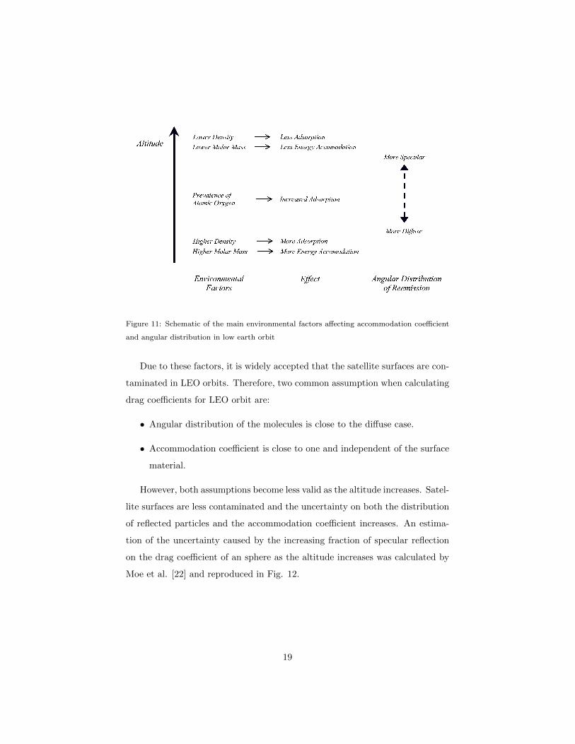
Angular distribution and accommodation coefficient vary with altitude due

to changes in atmospheric composition and, in the case of adsorption, changes

in density (Fig. 11). Adsorption is more pronounced at some altitudes since

some atmospheric constituents are more likely to be adsorbed than others. The

prime case of this is atomic oxygen [37], which is prevalent at altitudes between

approximately 200 and 700 km in mean solar conditions.

18

Gas-Surface Interaction Models

64

Laboratory experiments have shown that heavier molecules with a higher kinetic energy experience greater accommodation of momentum and energy than lighter molecules [17][19]. Therefore, heavier molecules are reemitted more diffusely. Consequently, the effect of increased molar mass at lower altitudes is to increase the extent of diffuse reflection.

Adsorption describes the process by which satellite surfaces in low Earth orbit become covered by atmospheric molecules that are trapped close to the surface [19]. The surface contamination caused by adsorption leads to an increase in energy accommodation (more energy is lost to the contaminated surface by incident molecules on impact). Therefore, the effect of adsorption is a broader angular distribution of reemitted molecules, which is closer to the diffuse case.

Figure 3-10 - Schematic of the Main Environmental Factors Affecting Accommodation Coefficients in Low Earth Orbit

Furthermore, laboratory experiments have demonstrated that in general,

clean, smooth surfaces produce a more specular distribution of reemitted molecules than rough, or contaminated surfaces, especially at higher incidences [17][74]. It is also worth noting that some authors have found that specular reemission is more likely with increasing surface temperature [15].

The effects of adsorption are more pronounced at some altitudes. There are two main reasons for this. Firstly, at higher altitudes, where the atmosphere is more rarefied, surface interaction is less frequent, such that fewer molecules are likely to be adsorbed. Secondly, atmospheric composition varies with altitude and some atmospheric constituents are more likely to be adsorbed than others.

Atomic oxygen is particularly likely to be adsorbed. This is because it is highly reactive with a wide variety of materials, causing corrosion by oxidisation and

Figure 11: Schematic of the main environmental factors affecting accommodation coefficient

and angular distribution in low earth orbit

Due to these factors, it is widely accepted that the satellite surfaces are con-

taminated in LEO orbits. Therefore, two common assumption when calculating

drag coefficients for LEO orbit are:

• Angular distribution of the molecules is close to the diffuse case.

• Accommodation coefficient is close to one and independent of the surface

material.

However, both assumptions become less valid as the altitude increases. Satel-

lite surfaces are less contaminated and the uncertainty on both the distribution

of reflected particles and the accommodation coefficient increases. An estima-

tion of the uncertainty caused by the increasing fraction of specular reflection

on the drag coefficient of an sphere as the altitude increases was calculated by

Moe et al. [22] and reproduced in Fig. 12.

19

molecules with the long sides, as a consequence of therandom thermal components of the incoming velocityvector.

The computed drag coefficients of compact satelliteshave a large dependence on altitude (Fig. 1) because thespeed ratio decreases with increasing altitude, while thedecreasing surface coverage causes the accommodationcoefficients to decrease. Drag coefficients also have asmall dependence on time in the sunspot cycle (Moe etal., 1995) through the temperature and mean molecularmass. Table 2 indicates the effects of accommodationcoefficient, local temperature, and mean molecular masson the drag coefficient of a short cylinder capped by aflat plate that faces the airstream. The incident velocityvector is along the axis of the cylinder which has a lengthto diameter ratio of 1. The reemission is assumed to beentirely diffuse (Moe et al., 1995).

5. Gas–surface interactions at higher altitudes

If we want to improve the calculation of dragcoefficients at higher altitudes, we must have informa-tion on how gas–surface interactions change characteras the amount of atomic oxygen adsorbed on satellitesurfaces decreases with increasing altitude. We know

from laboratory experiments that as the surfacecontamination decreases, the energy accommodationcoefficients decrease and the angular distribution ofreemitted molecules has an increasingly importantquasi-specular component (Saltsburg et al., 1967). Anestimate of the uncertainty in drag coefficient caused bythe quasi-specular component is shown in Fig. 2. Thiscomponent was estimated by using Schamberg’s(1959a, b) model, in which the quasi-specular compo-nent was chosen to be twice the quasi-specularcomponent measured by Gregory and Peters (1987), inorder to obtain an upper bound. However, themomentum transfer caused by the incoming streamwas still taken from Sentman’s analysis. The completelydiffuse case was calculated entirely from Sentman’s(1961a) model, as in Fig. 1.

To use a model of drag coefficients above 300 km, weneed data on accommodation coefficients from satellitesat higher altitudes. In a pioneering effort, Harrison andSwinerd (1995) performed a multiple satellite analysis at800–1000 km. Using satellites of various shapes andorientations, they found evidence of lower energyaccommodation and more quasi-specular reemissionthan measured at the lower altitudes. In a similarmanner, the data on many satellites such as thosecollected by the USAF High-Accuracy Satellite Drag

ARTICLE IN PRESS

Table 2Drag coefficients of a short cylinder capped by a flat plate (L/D ! 1)

Local temperature (K) Atmospheric mean molecular mass (amu) Accommodation coefficient

a ! 1:00 a ! 0:95 a ! 0:90

500 18 2.33 2.55 2.68500 22 2.30 2.53 2.661000 18 2.42 2.65 2.771000 22 2.38 2.61 2.741500 18 2.50 2.72 2.851500 22 2.45 2.68 2.81

Fig. 2. Uncertainties in drag coefficient caused by quasi-specular reemission. The solid curves represent drag coefficients calculated using Sentman’smodel, which assumes completely diffuse reemission. The dashed curves represent our estimated upper bound on the effect of a quasi-specularcomponent of reemission on the drag coefficient. As in Fig. 1, 2.2 has been widely used for all compactly shaped satellites.

K. Moe, M.M. Moe / Planetary and Space Science 53 (2005) 793–801 797

Figure 12: Uncertainties in drag coefficient caused by quasi-specular remission. Reproduced

from [22]

.

4. Solving the problem

4.1. Analytical Methods

Two common approaches are presented here, Schamberg [32] and Schaaf

and Chambre [30] . They represent two different ways of obtaining analytical

expressions for the drag and lift coefficients of convex bodies in FMF . To some

extent, almost all the derivations and applications of spacecraft aerodynamic

modelling in the literature are based on one of these two models.

4.1.1. Schamberg’s derivation

Schamberg [32] derives analytical expressions for the drag coefficient for

different elementary shapes in hyperthermal flow based on his GSIM (presented

in section 3.2). The resulting expressions are complex and depend upon the

GSIM coefficients. The resulting reflected fluxes for a flat plate can be obtained

with the help of Fig. 10:

pr = ρV 2i sin2 θiΦ(φ0)

VrVi

sin θrsin θi

(20)

τr = ρV 2i sin θi cos θiΦ(φ0)

VrVi

sin θrsin θi

(21)

20

Eq. (22) presents the general form of Schamberg’s hyperthermal drag coefficient

for all shapes based on projected area.

CD = 2

[1 + Φ(φ0)

VrVif(ν, shape)

](22)

The parameters ν and Φ(φ0) are the same ones defined in section 3.2. The

ratio Vr/Vi (reflected and incident molecule velocities) can be related with the

accommodation coefficient as follows [26] (notice the constant reflected velocity

assumption):

α =Ei − ErEi − Ew

=12mV

2i − 1

2mV2r

12mV

2i − Ew

(23)

Assuming that the ratio Ew/(1/2mV2i ) is numerically negligible we can relate

the velocity ratio (r) and the accommodation coefficient:

r =VrVi

=√

1− α (24)

Generally, for practical applications, the definition of ν and φ0 is difficult and

some further simplifications are needed. We can fix these values to their diffuse

and specular extremes resulting in two different expressions for quasi-specular

and quasi-diffuse reflections, since they will still depend on the accommodation

coefficient. Shamberg’s quasi-diffuse model based on the hyperthermal assump-

tion has been very popular. Cook [8] used this model in what has become a

key reference to calculate satellite drag coefficients. He calculates r in a sightly

different way:

r =VrVi

=

(ErEi

)1/2

=

{1 + α

(EwEi− 1

)}1/2

(25)

EwEi

=TwTk,i

(26)

Where Tw is the already defined wall temperature and Tk,i = 1/(3R)V 2i is

21

SATELLITE DRAG COEFFICIENTS 937

of 50-60 eV being quoted for most materials. With the more accurate measuring techniques now available, very small yields have been measured at lower energies. Extrapolation of these results(l*) suggests that sputtering is insignificant at energies below 20-25 eV. It is therefore reasonable to conclude that sputtering will have a negligible effect on drag, both directly through the removal of momentum by sputtered material, and indirectly through the modification of ,LJ by the removal of adsorbed atoms. McKeown and his collaboratorsug) claim to have measured sputtering on two Discoverer satellites at a height of about 200 km. The erosion rates were found to be O-1 5 0.05 A/day for gold and O-15 & 0.05 A/day for silver, corresponding to sputtering yields of 10d6 atoms/molecule and 2 x 1OP atoms/mole- cule respectively. These values have recently been disputed,(20) however.

4. DRAG OF SIMPLE SHAPES IN HYPERTHERMAL FREE-MOLECULE FLOW From equation (5) the ratio of the speed of a re-emitted molecule v, to the speed of an

incident molecule vi is related to the thermal accommodation coefficient by the equations

;=(y=(l++l))” ] and (8)

Es _ Tw E,-Ti'

where Ti is the kinetic temperature of incidence and T, is the surface temperature. Since we are unable to make any statement about the variation of tc with the angle of incidence of a surface element, all reflected molecules are assumed to have the same value of v,. After making this assumption, there is little point in taking into account the random thermal motion in detail for molecular speed ratios above 5.

The drag of satellites in hyperthermal free-molecule flow has been studied by Schamberg(5) and his results for certain simple shapes are quoted in Table 1. The drag coefficient C, is defined by

D c,=-, &p v2s

TABLE 1. DRAG IN HYPERTHERMAL FREE-MOLECULE FLOW

Drag coefficient

Shape (based on projected area perpendicular to direction

of motion)

Diffuse re-emission Accommodated specular

reflexion Flat plate

(normal to flow) 2(1 + fr) 2(1 + r)

Flat plate at incidence 0 2 ( 1 +irsinO 1

21+$ ( 1 Cylinder perpendicular

to flow Cone of semi vertex

angle y with vertex forwards and axis parallel to flow

2 . 2(1 +?rsmy 2(1 - r cos 2yr)

Figure 13: Schamberg’s quasi-specular and quasi diffuse drag coefficients for simple geometries

(based on projected area). Reproduced from [8]

the kinetic temperature. Fig. 13 offers drag coefficients for different shapes

for quasi-diffuse and quasi-specular reflections under hyperthermal conditions.

Notice that this model provides with a description of the angular distribution

of the reflected particles. Schamberg’s model is a very adaptive model capable

of describing a wide range of different scattering patterns. However, besides

the two extreme cases, diffuse and specular, it is not straightforward to define

the parameters of the model when trying to predict real satellite conditions,

moreover it assumes a constant speed distribution. Therefore, calculations of

satellite drag using this model are restricted to one of the two limiting cases, and

although intuitive, the validity of such an assumption is not clear [26]. Some

practical applications of the Schamberg’s model can be found in [35] and [21].

4.1.2. Schaaf and Chambre derivation

From Eqs. (18) and (19) we can obtain the reflected fluxes by means of the

momentum accommodation coefficients as follows:

pr = (1− σN )pi + σNpw (27)

τr = (1− σT )τi (28)

Using the above relations together with Eqs. (9 - 10) it is possible to derive a

general expression for the pressure and shear stress coefficients for a flat plate

22

with one side exposed to the flow. For the complete derivation, including the

calculation of pw refer to [30]. The coefficients are given by (the reference area

is the total area of the plate):

Cp =1

s2

{(2− σN ) Γ1(s cos δ) +

σN2

(TwTinf

)1/2√π Γ2(s cos δ)

}(29)

Cτ =σT sin δ

sΓ2(s cos δ) (30)

Where Tw is the surface temperature and Tinf the ambient temperature, the

Γ functions are the ones defined in Eqs. (11 - 12). Notice that there is no

restriction on the angle of incidence δ therefore it may take values greater than

90 deg. In this scenario, the surface is aft facing. However, it may still be

impacted by molecules that have large lateral thermal velocities in comparison

to the bulk velocity vector.

Eqs. (29) and (30) depend on the two momentum accommodation coeffi-

cients (σN , σT ). They are meant to be determined by experiments, however,

this approach is also far from being perfect: orbital conditions are hard to re-

produce on earth facilities and orbital experiments are expensive and difficult

to carry out. The reality is that little data have been gathered in representa-

tive conditions and a number of assumptions have to be made in order to give

values to the coefficients. For a review of some experimental and theoretical

approaches to determine these coefficients for different gases, surfaces and an-

gles of incidence refer to [12, 13] . Two practical cases, the determination of

the CHAMP and ANS-1 aerodynamic databases, and the assumptions made to

calculate the accommodation coefficients can be found in [26] and [18].

Alternative expressions for the force coefficients can be found in the liter-

ature. Storch [34] provides a very clear and easy to follow derivation of these

equations, Sentman [33] assumes diffuse reflection and uses the temperature of

the reflected molecules (Tr) to account for incomplete thermal accommodation.

Moe et al [24] modify Sentman’s expressions to include the thermal accommo-

dation coefficient instead of Tr. The different analytical formulations in the

23

literature cannot always be reconciled. Care must be taken since it is criti-

cal to understand the basic assumptions under each of the formulas prior to

producing any result. Some mistakes have been reported in the calculation of

drag coefficients: confusion of kinetic and atmospheric temperatures in Cook’s

formula or incorrect hyperthermal assumption for certain flight conditions and

body shapes [15].

Whereas the pressure coefficient has a unique definition, the drag and lift

coefficients depend on the reference area chosen for the calculation. It is a

common practice to use the projected area that varies with the incidence angle

instead of a fixed area (however, the product SCD and hence the drag force are

still the same regardless of the reference area chosen). A fixed reference area is

preferred when building aerodynamic databases for dynamic simulations since it

simplifies the calculation to retrieve the force. A projected reference area gives

a better idea of the aerodynamic performance since it excludes the variation of

projected area from CD. It allows the comparison of CD for different vehicles

or configurations.

An important comment is that different accommodation coefficients are as-

sociated with different gas-species, since different gas-surface interation is ex-

pected depending on the molecular characteristics of the gas. The atmosphere

is a mixture of gases, and the drag coefficient is different for each constituent.

Therefore, the drag force should be calculated taking into account a different

drag coefficient for each species [12]. In practice, a different drag coefficient

for each gas species introduces further uncertainties in the problem, a common

approach being to use the mean molecular mass at the altitude of interest.

Besides the simple flat plate formula, it is also possible to derive analytical

solutions of the force coefficients for some simple geometric shapes. The deriva-

tion consists on integrating the coefficients equations for an element of area over

the surface of the body; see [34, 33, 31]. The analytical solutions are therefore

limited to simple convex bodies such as spheres, cones, cylinders, etc.

24

4.2. Numerical Methods

For more complex bodies, the aerodynamic coefficients have to be calculated

by means of numeric methods. There are four main computational methods for

analysing the aerodynamics of a body in free molecular flow:

• Panel Method

• Ray-Tracing Panel Method (RTP)

• Test-Particle Monte Carlo (TPMC)

• Direct Simulation Monte Carlo (DSMC)

They are compared in Fig. 14, along with the Computational Fluid Dynamics

(CFD) method that is used in continuum flow. The right-hand axes of Fig. 14

represent both the free stream molecular speed ratio s and free stream Knudsen

number Kn. The Knudsen number is based on a spacecraft with a characteristic

dimension of 5 m. The different regimes of rarefied flow are indicated using the

Knudsen number scale.

4.2.1. Panel Method

A body may be idealised as being made up of a number of discrete panels

that can each be modelled as a flat plate with one side exposed to the flow. The

pressure and shear stress for each panel can then be calculated using any of the

available forms of the expressions for CP and Cτ for a flat plate in FMF. Then,

adding the contributions of the n panels all together it is possible to calculate

the body force coefficient [29]:

CF =

n∑i=1

CPi(−~ni) + Cτi

~ni × ~V∣∣∣~V ∣∣∣ × ~ni

AiAref

(31)

In hyperthermal flow only forward facing panels (0 ≤ δ ≤ π/2) contribute to

the body force coefficients. In contrast in hypothermal flow all panels may be

impacted regardless of whether they are forward facing or not (0 ≤ δ ≤ π). This

25

Spacecraft Aerodynamics

34

Figure 2-16 - Comparison of Existing Computational Approaches to Spacecraft Aerodynamics in Low Earth Orbit

Assumes mean solar conditions (as defined by [18]) and a free stream Knudsen number (Kn) based upon a spacecraft characteristic dimension of 5 m. The term h refers to Earth altitude

and s refers to the free stream molecular speed ratio. The Computing Time, Developer Expertise Required, and User Expertise Required scales are based upon a qualitative survey of numerous rarefied gas dynamics texts (see, for example, [27]). They are provided as a “rule of

thumb,” without quantative explanations save those given in the following sections and chapters.

Other aspects of Figure 2-16, including the different terms and various computational analysis methods depicted, will be described in more detail in the following sections.

2.6.1 Panel Method

As explained in previous sections, in free molecular flow, intermolecular collisions can be neglected, such that a body may be seen as having no influence on its upstream flow field.

Therefore, a body may be idealised as being made up of a number of discrete panels that can each be modelled as a flat plate subject to a chosen Gas-Surface

Figure 14: Comparison of existing computational approaches to spacecraft aerodynamics in

low earth orbit

26

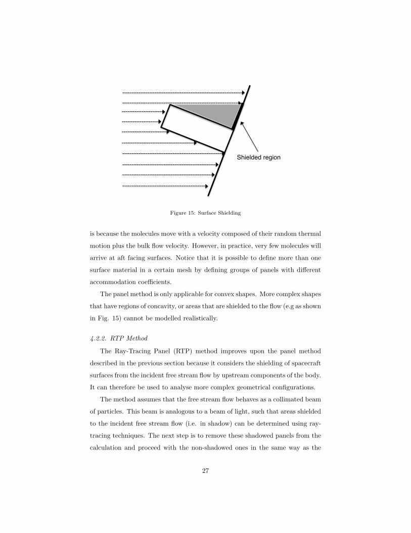
Shielded region!

Figure 15: Surface Shielding

is because the molecules move with a velocity composed of their random thermal

motion plus the bulk flow velocity. However, in practice, very few molecules will

arrive at aft facing surfaces. Notice that it is possible to define more than one

surface material in a certain mesh by defining groups of panels with different

accommodation coefficients.

The panel method is only applicable for convex shapes. More complex shapes

that have regions of concavity, or areas that are shielded to the flow (e.g as shown

in Fig. 15) cannot be modelled realistically.

4.2.2. RTP Method

The Ray-Tracing Panel (RTP) method improves upon the panel method

described in the previous section because it considers the shielding of spacecraft

surfaces from the incident free stream flow by upstream components of the body.

It can therefore be used to analyse more complex geometrical configurations.

The method assumes that the free stream flow behaves as a collimated beam

of particles. This beam is analogous to a beam of light, such that areas shielded

to the incident free stream flow (i.e. in shadow) can be determined using ray-

tracing techniques. The next step is to remove these shadowed panels from the

calculation and proceed with the non-shadowed ones in the same way as the

27

panel method described above.

This method is only generally valid under hyperthermal conditions (s > 5).

When modelling convex bodies with no shielded surfaces in hypothermal flow

the random thermal motion of molecules is accounted for at the panel level in

the GSIM. However, when modelling complex bodies with shielded surfaces,

these are identified and removed from the calculation. Such a simplification as-

sumption is no longer valid in hypothermal flow, so this method looses accuracy

in this regime.

4.2.3. TPMC Method

The Test-Particle Monte Carlo (TPMC) is a step further with respect to

panel methods. It was first proposed by Davis in 1961 [10]. In TPMC, the

model is surrounded by a control tube into which a number of representative

particles are sequentially fired. Each particle represents many thousands of real

molecules. These test-particles, or simulated molecules, can be emitted from all

sides of the control tube to mimic the characteristics of the real flow. Therefore,

TPMC can be used to model the effects of multiple reflections and different

flow conditions. The particles can reflect off the surfaces of the model, but

do not interact with one another. Notice that this method needs a model of

the scattering pattern of the reflected molecules (such as the ones developed by

Maxwell or Schamberg).

The consequences of neglecting the effects of multiple reflections can be

visualised with the help of Fig. 16; using the Panel or the RTP methods, the

calculation of the force exerted on Surface A would yield the same result as

the calculation of the force exerted on Surface B (assuming equivalent surface

areas). Yet, in reality, the force exerted on Surface B would be less than the

force exerted on Surface A because the surfaces of Surface A would be impacted

by reflected flow in addition to free stream flow.

28

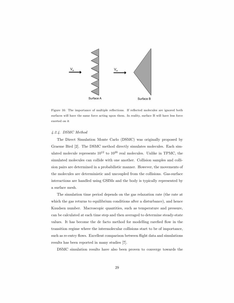
Surface A Surface B

Va Va

Figure 16: The importance of multiple reflections. If reflected molecules are ignored both

surfaces will have the same force acting upon them. In reality, surface B will have less force

exerted on it

4.2.4. DSMC Method

The Direct Simulation Monte Carlo (DSMC) was originally proposed by

Graeme Bird [2]. The DSMC method directly simulates molecules. Each sim-

ulated molecule represents 1012 to 1020 real molecules. Unlike in TPMC, the

simulated molecules can collide with one another. Collision samples and colli-

sion pairs are determined in a probabilistic manner. However, the movements of

the molecules are deterministic and uncoupled from the collisions. Gas-surface

interactions are handled using GSIMs and the body is typically represented by

a surface mesh.

The simulation time period depends on the gas relaxation rate (the rate at

which the gas returns to equilibrium conditions after a disturbance), and hence

Knudsen number. Macroscopic quantities, such as temperature and pressure,

can be calculated at each time step and then averaged to determine steady-state

values. It has become the de facto method for modelling rarefied flow in the

transition regime where the intermolecular collisions start to be of importance,

such as re-entry flows. Excellent comparison between flight data and simulations

results has been reported in many studies [7].

DSMC simulation results have also been proven to converge towards the

29

Boltzmann equation [3]. Therefore, in theory, DSMC could be used to model

flow in the continuum regime too. However, its computational load is directly

proportional to the density of the gas. In the lower transition regime and con-

tinuum regime, this makes it prohibitively expensive in computational terms at

the current time, especially for complex three dimensional bodies.

5. Conclusion

Although more than 60 years have passed since the first satellite was put in

orbit, the drag force prediction of an orbiting spacecraft is still a challenging

problem. There is still a requirement to improve our knowledge of the upper

atmosphere environment and our understanding of the gas-surface interaction

phenomena. An increase on the interest in the topic is noticeable in recent

years, both in the number of scientific missions with dedicated payloads and

the number of published papers. Different methods of different complexity and

accuracy have been reviewed in this paper to predict drag coefficients. Although

they all depend on the accuracy of the gas-surface interaction model which is

not always known, a comprehensive aerodynamic analysis of the spacecraft is of

indubitable value to analyse and interpret gathered experimental data, as well

as to study new ideas and proposals.

[1] Space engineering: Space environment, ECSS Std. ECSS-E-10-04A. ESA-

ESTEC, Noordwijk, The Netherlands, 2008.

[2] G. A. Bird. Molecular gas dynamics and the direct simulation of gas flows,

volume 42. Clarendon Press, Oxford, 1994.

[3] G. A. Bird. Forty years of DSMC, and now? In Rarefied Gas Dynamics:

22nd International Symposium, volume 585, page 372. American Institute

of Physics, 9/7/2000 2000.

[4] B. R. Bowman. The semiannual thermospheric density variation from 1970

to 2002 between 200-1100 km. In Advances in the Astronautical Sciences,

volume 119, pages 1135–1154, 2005.

30

[5] B. R. Bowman, W. K. Tobiska, F. A. Marcos, C. Y. Huang, C. S. Lin,

and W. J. Burke. A new empirical thermospheric density model JB2008

using new solar and geomagnetic indices. In AIAA/AAS Astrodynamics

Specialist Conference and Exhibit, 2008.

[6] B. R. Bowman, W. Kent Tobiska, F. A. Marcos, and C. Valladares. The

JB2006 empirical thermospheric density model. Journal of Atmospheric

and Solar-Terrestrial Physics, 70(5):774–793, 2008.

[7] I. D. Boyd. Direct simulation Monte Carlo for atmospheric entry: Code de-

velopment and application results. Technical Report EN-AVT-162, NATO

RTO Report, 2009.

[8] G. E. Cook. Satellite drag coefficients. Planetary and Space Science,

13(10):929–946, 1965.

[9] R. Crowther and J. Stark. The determination of the gas-surface interaction

from satellite orbit analysis as applied to ANS-1 (1975-70a). Planetary and

Space Science, 39(5):729–736, 1991.

[10] D. H. Davis. Monte Carlo calculation of molecular flow rates through a

cylindrical elbow and pipes of other shapes. Journal of Applied Physics,

31(7):1169–1176, 1960.

[11] E. Doornbos and H. Klinkrad. Modelling of space weather effects on satel-

lite drag. Advances in Space Research, 37(6):1229–1239, 2006.

[12] E. M. Gaposchkin and Coster A.J. Analysis of satellite drag. Lincoln

Laboratory Journal, 1:203–224, 1988.

[13] E. D. Knechtel and W. C. Pitts. Normal and tangential momentum accom-

modation for earth satellite conditions. Astronautica Acta, 18(3):171–184,

1973.

[14] S. H. Knowles, J. M. Picone, S. E. Thonnard, and A. C. Nicholas. The

effect of atmospheric drag on satellite orbits during the Bastille Day Event.

Solar Physics, 204(1-2):387–397, 2001.

31

[15] G. Koppenwallner. Comment on special section: New perspectives on the

satellite drag environments of Earth, Mars, and Venus. Journal of Space-

craft and Rockets, 45(6):1324–1327, 2008.

[16] F. A. Marcos, B. R. Bowman, and R. E. Sheehan. Accuracy of Earth’s

thermospheric neutral density models. In Collection of Technical Papers

- AIAA/AAS Astrodynamics Specialist Conference, 2006, volume 1, pages

422–441, 2006.

[17] F. A. Marcos, W. J. Burke, and S. T. Lai. Thermospheric space weather

modeling. In Collection of Technical Papers - 38th AIAA Plasmadynamics

and Lasers Conference, volume 2, pages 999–1010, 2007.

[18] D. D. Mazanek, R. R. Kumar, M. Qu, and H. Seywald. Aerothermal analy-

sis and design of the Gravity Recovery and Climate Experiment (GRACE)

spacecraft. NASA Technical Memorandum, (210095):XI–42, 2000.

[19] D. D. Mazanek, R. R. Kumar, and H. Seywald. GRACE mission design:

Impact of uncertainties in disturbance environment and satellite force mod-

els. In AAS/AIAA Space Flight Mechanics Meeting, volume AAS 00, page

163, 2000 2000.

[20] K. Moe. Six reasons why thermospheric measurements and models disagree.

In M. H. Davis, Smith R.E., and Johnson D.L., editors, NASA Conference

Publication, volume 2460, pages 291–303, feb 1987.

[21] K. Moe and B. R. Bowman. The effects of surface composition and treat-

ment on drag coefficients of spherical satellites. In Advances in the Astro-

nautical Sciences, volume 123 I, pages 137–152, 2006.

[22] K. Moe and M. M. Moe. Gas-surface interactions and satellite drag coeffi-

cients. Planetary and Space Science, 53(8):793–801, 2005.

[23] K. Moe and M. M. Moe. Gas-Surface Interactions in Low-Earth Orbit. In

American Institute of Physics Conference Series, volume 1333 of American

Institute of Physics Conference Series, pages 1313–1318, May 2011.

32

[24] K. Moe, M. M. Moe, and C. J. Rice. Simultaneous analysis of multi-

instrument satellite measurements of atmospheric density. Journal of

Spacecraft and Rockets, 41(5):849–853, 2004.

[25] Oliver Montenbruck and Eberhard Gill. Satellite orbits: models, meth-

ods, and applications. Springer, Berlin, 2000. by Oliver Montenbruck and

Eberhard Gill.; AERO.

[26] P. Moore and A. Sowter. Application of a satellite aerodynamics model

based on normal and tangential momentum accommodation coefficients.

Planetary and Space Science, 39(10):1405–1419, 1991.

[27] J. F. Padilla. Assessment of gas-surface interaction models for computation

of rarefied hypersonic flows, 2008.

[28] J. M. Picone, A. E. Hedin, D. P. Drob, and A. C. Aikin. NRLMSISE-00

empirical model of the atmosphere: Statistical comparisons and scientific

issues. Journal of Geophysical Research A: Space Physics, 107(A12), 2002.

[29] F. J. Regan and Satya M. Anandakrishnan. Dynamics of atmospheric re-

entry. American Institute of Aeronautics and Astronautics, Washington,

DC, 2 edition, 1993. Frank J. Regan, Satya M. Anandakrishnan.; SPEC-

BOOKS; ASE.

[30] S. A. Schaaf and P. L. Chambre. Flow of rarefied gases, volume 8. Princeton

University Press, Princeton, NJ, 1961.

[31] S. A. Schaaf and L. Talbot. Mechanics of rarefied gases, volume 5 of Hand-

book of Supersonic Aerodynamics, chapter 16. Bureau of Naval Weapons

U.S Navy, 1959.

[32] R. Schamberg. A new analytic representaticn of surface interaction with

hypothermal free molecule flow with application to neutral-particle drag

estimates of satellites. Technical Report RM-2313, RAND Research Mem-

orandum, 1959.

33

[33] L. H. Sentman. Free Molecule Flow Theory and Its Application to the Deter-

mination of Aerodynamic Forces. Lockheed Missiles and Space Company,

Lockheed Aircraft Corporation, 1961.

[34] J. A. Storch. Aerodynamic disturbances on spacecraftin free-molecular flow

(monograph). Technical report, The Aerospace Corporation, 2002.

[35] B. D. Tapley, J. C. Ries, S. Bettadpur, and M. Cheng. Neutral density

measurements from the grace accelerometers. In Collection of Technical

Papers - AIAA/AAS Astrodynamics Specialist Conference, 2006, volume 1,

pages 484–494, 2006.

[36] K. F. Tapping. Recent solar radio astronomy at centimeter wavelengths:

The temporal variability of the 10.7-cm flux. Journal of Geophysical Re-

search, 92:829–838, January 1987.

[37] R. C. Tennyson. Atomic oxygen and its effect on materials in space. In

International Symposium on Rarefied Gas Dynamics, volume 160, page

461, Vancouver, Canada, 31/7/1992 1992. AIAA, Rarefied Gas Dynamics:

Space Science and Engineering.

[38] D. A. Vallado and D. Finkleman. A critical assessment of satellite drag and

atmospheric density modeling. In AIAA/AAS Astrodynamics Specialist

Conference and Exhibit, 2008.

[39] H. Y. Wachman. The thermal accommodation coefficient: A critical survey.

Technical report, Space Sciences Laboratory, Missile and Space Vehicle

Department, General Electric, 1961.

[40] Dean C. Wadsworth, Douglas B. Vangilder, and Virendra K. Dogra. Gas-

surface interaction model evaluation for DSMC applications. In Rarefied

Gags Dynamics: 23rd International Symposium, volume 663, page 965.

American Institute of Physics, 20/7/2002 2003.

[41] R. L. Walterscheid. Solar cycle effects on the upper atmosphere - implica-

tions for satellite drag. In AIAA, Aerospace Engineering Conference and

34

Show, volume 26, pages 439–444. Journal of Spacecraft and Rockets, Feb.

14-16, 1989 1989.

[42] M. D. Zettergren, W. L. Oliver, P. L Blelly, and D. Alcayd. Modeling the

behavior of hot oxygen ions. Annales Geophysicae, 24(6):1625–1637, 2006.

35

List of Figures

1 Variation of the mean atmospheric density with altitude for low,

moderate and high solar and geomagnetic activities as defined by

JB2006 model. Reproduced from [1] . . . . . . . . . . . . . . . . 5

2 Variation of the Earth’s atmospheric composition with altitude

as defined by NRLMSISE00 model. Reproduced from [1] . . . . . 6

3 Molecular Mean Free Path (λ) . . . . . . . . . . . . . . . . . . . 8

4 Knudsen number variation with altitude for low, moderate and

high solar and geomagnetic activities using NRLMSISE-00, and

a characteristic dimension of 1 m . . . . . . . . . . . . . . . . . . 9

5 Classification of flow regimes using Knudsen number. Repro-

duced from [2] . . . . . . . . . . . . . . . . . . . . . . . . . . . . . 9

6 Hyperthermal (s→∞) and hypothermal (s <<∞) flows . . . . 11

7 Impact on parallel surface due to random thermal motion of the

flow molecules . . . . . . . . . . . . . . . . . . . . . . . . . . . . . 11

8 Incident and reflected fluxes on a convex element of area . . . . . 12

9 Specular and diffuse reflected fluxes . . . . . . . . . . . . . . . . 15

10 Schamberg’s GSIM . . . . . . . . . . . . . . . . . . . . . . . . . . 17

11 Schematic of the main environmental factors affecting accommo-

dation coefficient and angular distribution in low earth orbit . . . 19

12 Uncertainties in drag coefficient caused by quasi-specular remis-

sion. Reproduced from [22] . . . . . . . . . . . . . . . . . . . . . 20

13 Schamberg’s quasi-specular and quasi diffuse drag coefficients for

simple geometries (based on projected area). Reproduced from [8] 22

14 Comparison of existing computational approaches to spacecraft

aerodynamics in low earth orbit . . . . . . . . . . . . . . . . . . . 26

15 Surface Shielding . . . . . . . . . . . . . . . . . . . . . . . . . . . 27

16 The importance of multiple reflections. If reflected molecules are

ignored both surfaces will have the same force acting upon them.

In reality, surface B will have less force exerted on it . . . . . . . 29

36