spacecraft dynamics and control - an introduction exercises · spacecraft dynamics and control - an...
TRANSCRIPT
Spacecraft Dynamics and Control- An Introduction
EXERCISES
Anton H.J. de Ruiter, Christopher J. Damaren and James R. Forbes

This document contains exercises to accompany the book. Theauthors welcome anyfeedback. Please send any comments, corrections or suggestions to [email protected].
CONTENTS
1 Chapter 1 Exercises 5
2 Chapter 2 Exercises 27
3 Chapter 3 Exercises 33
4 Chapter 4 Exercises 39
5 Chapter 5 Exercises 43
6 Chapter 6 Exercises 45
7 Chapter 7 Exercises 49
8 Chapter 9 Exercises 55
9 Chapter 10 Exercises 59
10 Chapter 12 Exercises 61
11 Chapter 13 Exercises 65
12 Chapter 14 Exercises 67
13 Chapter 15 Exercises 69
14 Chapter 16 Exercises 71
15 Chapter 17 Exercises 73
16 Chapter 18 Exercises 77
17 Chapter 19 Exercises 79
18 Chapter 20 Exercises 81
19 Bias Momentum Control Design Exercises - Chapters 17 to 20 83

4 CONTENTS
20 Chapter 21 Exercises 89
21 Chapter 22 Exercises 91
22 Chapter 25 Exercises 95

1Chapter 1 Exercises
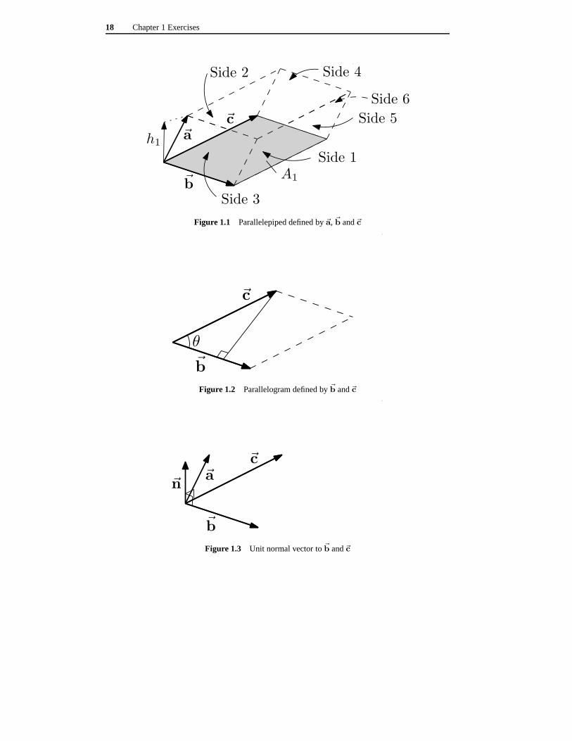
1. Consider three non-coplanar vectors~a, ~b and~c, as shown in Figure 1.1, which definea parallelepiped.
Note that all sides are parallelograms, and that opposing sides are parallel. Note thatas drawn, the vector~a points above the plane defined by vectors~b and~c. The volumeof the parallelepiped is given by the area of any one of its sides, multiplied by theperpendicular distance to the opposing side. In terms of figure 1.1,
V = A1h1 (1.1)
(a) Consider the parallelogram defined by vectors~b and~c, as shown in Figure 1.2.
Determine the areaA1 in terms of~b and~c.
(b) Referring to figure 1.3, determine the vector~n of unit magnitude (|~n| = 1) thatis perpendicular to the parallelogram defined by~b and~c, and points to the sameside of it as the vector~a.
(c) Using the result from (b), determine the perpendicular distance from side 1 to theopposing side 4, in terms of the vectors~a and~n.
(d) Using equation (1.1), compute the volume,V of the parallelepiped in terms ofthe vectors~a, ~b and~c.
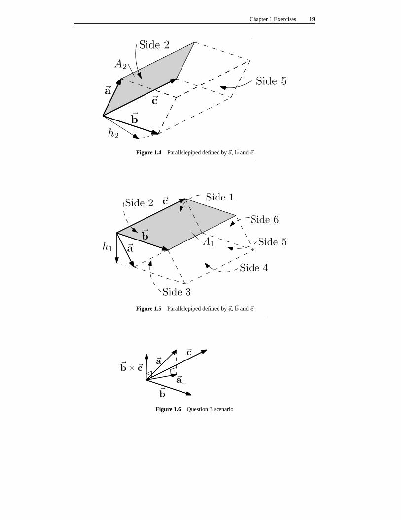
(e) Referring to figure 1.4, compute the volume using the areaof side 2 (A2),multiplied it by the perpendicular distance (h2) from side 2 to side 5, that isV = A2h2.
(f) Combine the results of (d) and (e).
2. Consider again three non-coplanar vectors~a, ~b and~c, as shown in Figure 1.5, whichdefine a parallelepiped. Note that unlike in Figure 1.1, the vector~a points below theplane defined by vectors~b and~c.
(a) Repeat parts (a) to (f) of Question 1, using the parallelepiped shown in Figure1.5.
(b) Now, consider three co-planar vectors~a, ~b and~c. Compute~a · (~b× ~c) and~b · (~c× ~a). What can you conclude from this and part (f) in Question 1 andpart (a) in this question?
Spacecraft Dynamics and Control - An Introduction,Anton H.J. de Ruiter, Christopher J. Damaren and James R. Forbes,c© 2013 John Wiley & Sons, Ltd. Published 2013 by John Wiley & Sons, Ltd.
Companion Website: http://www.wiley.com/go/deruiter/spacecraft

6 Chapter 1 Exercises
3. Consider the vectors~a, ~b and~c. In this problem, you are going to find an alternativeexpression for~a× (~b× ~c). It is assumed that~a, ~b and~c are non-zero, and non parallel(see figure 1.6).
It has been shown that~a× (~b× ~c) = ~a⊥ × (~b× ~c), where~a⊥ is the component of~athat is perpendicular to~b× ~c, such that~a = ~a⊥ + ~a‖ (where~a‖ is parallel to~b× ~c).
The vectors~b and~c define the plane that is perpendicular to~b× ~c. Therefore,~a⊥ mustlie in that plane.
(a) Consider the vectors~b and~c. Referring to figure 1.7, find~c‖b, the component of~cthat is parallel to~b. Using this, find~c⊥b, the component of~c that is perpendicularto ~b. Finally, find|~c⊥b| in terms of|~b× ~c| and|~b|.
(b) Since~b and~c⊥b are perpendicular, we may obtain the unit perpendicular vectors
~n1 =~b
|~b|, ~n2 =
~c⊥b|~c⊥b|
.
These vectors can also be used to define the plane containing~b and~c.
Use your solution to part (a) to find~n2 in terms of~b,~c, |~b| and|~b× ~c|.(c) The projection of the vector~a onto the plane defined by~b and~c is given by
~aproj = (~a · ~n1)~n1 + (~a · ~n2)~n2. (1.2)
Clearly,~aproj is perpendicular to~b× ~c, since it lies in the plane defined by~band~c.Show that the vector~a− ~aproj is perpendicular to the plane, and hence is parallelto ~b× ~c. Hint: Check(~a− ~aproj) · ~n1 and(~a− ~aproj) · ~n2.
Conclude from this that the component of~a parallel to ~b× ~c is given by~a‖ = ~a− ~aproj , while the component of~a perpendicular to~b× ~c is given by~a⊥ = ~aproj .
(d) Since~a⊥ is perpendicular to~b× ~c, the cross-product~a⊥ × (~b× ~c) is obtainedby rotating~a⊥ by 90o about~b× ~c, and then scaling by|~b× ~c|. That is,
~a⊥ × (~b× ~c) = ~a⊥rot|~b× ~c|, (1.3)
where~a⊥rot is the vector~a⊥ rotated by 90o in the direction indicated in Figure1.8.Consider the vectors~n1 and~n2. What are~n1rot and~n2rot, the vectors obtainedby rotating~n1 and~n2 by 90o respectively, as indicated in figure 1.9?Using this and (1.2), find~a⊥rot.
(e) Substitute the results from part (b) into~a⊥rot obtained in part (d), and finallyobtain the expression for~a× (~b× ~c) = ~a⊥ × (~b× ~c), using (1.3).
4. We have seen that for a right-handed reference frameF , the cross-product of twovectors~a = ~FTa and~b = ~FTb, is
~a× ~b = ~FTa×b,

Chapter 1 Exercises 7
where
a =
axayaz
, b =
bxbybz
, a×∆=
0 −az ayaz 0 −ax−ay ax 0
.
Determine the expression for~a× ~b if the frameF is left-handed (see figure 1.10). Youmay start from the expression
~a× ~b =[
ax ay az]
~x× ~x ~x× ~y ~x× ~z~y × ~x ~y × ~y ~y × ~z~z× ~x ~z× ~y ~z× ~z
bxbybz
.
5. A five-link robotic manipulator is being designed, with a hand at the end (see Figure1.11). Each of the links have the same length, given byr. Each of the joints allows arotation about a single axis. The vector~rij denotes the position of jointj relative tojoint i. The vector~rH denotes the position of the hand relative to the base of the robot(joint 1). Refer to Figure 1.11.
We attach a reference frame to the room, denoted byFr. This frame is defined with the~xr and~yr axes in the plane of the floor, and the~zr axis pointing vertically upwards.Refer to Figure 1.12.
It will also be useful to attach a reference frame to each link, denoted by~Fi, fori = 1, ..., 5. The reference frame attached to each link is defined such that the~zi axispoints along the length of the link from jointi to joint i+ 1. Refer to Figure 1.13. Thejoint rotations are:- Joint 1 allows a rotationθ1 about the~yr axis. See figure 1.14.- Joint 2 allows a rotationθ2 about the~x1 axis. See figure 1.15.- Joint 3 allows a rotationθ3 about the~z2 axis.- Joint 4 allows a rotationθ4 about the~y3 axis.- Joint 5 allows a rotationθ5 about the~z4 axis.
(a) Determine the vectors~r12,~r23,~r34,~r45,~r5H , in their respective link frames,F1,F2, F3, F4, F5.
(b) What is the orientation of the hand relative to the room coordinates? (Find therotational transformation fromFr to F5).
(c) Determine the position of the hand relative to the robot base,~rH , in roomcoordinatesFr. Note: leave your answer in terms of products of principal rotationmatrices.
The results from parts (b) and (c) will allow the robot user todetermine the requiredjoint anglesθ1, θ2, θ3, θ4, θ5 required to pick up an object with a given location andorientation.
6. Earth orbiting spacecraft problems often require the conversion between differentreference frames. Three frames that are often used are the Earth-Centered-Inertial(ECI) frame (denotedFG), the Earth-Centered-Earth-Fixed (ECEF) frame (denotedFF ) and the local Topocentric frame (denotedFT ). The ECI frame is an inertiallyfixed frame (does not rotate with the earth), with thez-axis is aligned with the earth’s

8 Chapter 1 Exercises
spin axis, and therefore thex- andy-axes lie in the equatorial plane. The origin of theECI frame is at the center of the earth. The ECEF frame also hasits origin at the centerof the earth, and thez-axis aligned with the earth’s spin axis. Thex-axis points to thelocation on the equator with zero longitude. Since the ECEF frame is fixed to the earth,thex- andy-axes rotate with the earth. The Topocentric frame depends on the locationon the surface of the earth, given by longitudeλ and latitudeδ. The origin is at thesurface of the earth, at the location of it’s definition. Itsx-axis points south along thelocal horizon, and it’sy-axis points toward the east along the local horizon. This frameis important, because it is within this frame that observations of a satellite are madefrom the Earth (with a telescope or radar for example).
The ECEF frame is obtained by a rotationθGMT = ωearth(t− t0) (called theGreenwich Mean Time) about the ECIz-axis. Note thatωearth is the earth’s rate ofrotation. See Figure 1.17.
The Topocentric frame is obtained by a rotationλ about the ECEFz-axis, followed bya rotation90o − δ about the transformedy-axis. See Figure 1.18.
(a) Determine the rotation matrix defining the transformation from ECEF to ECIcoordinates, and from Topocentric to ECI coordinates, thatis, determineCGF
andCGT . Hint: You may use the fact thatCz(a)Cz(b) = Cz(a+ b).(b) A ground satellite monitoring station with coordinatesλ, δ measures the position
of a satellite in local topocentric coordinates as~ρ = ~FTT ρ (see Figure 1.19).
Assuming that the Earth is a sphere with radiusRearth, show that the inertialposition~r = ~FT
Gr in ECI coordinates is given by:
r =
x sin δ cos(λ+ θGMT )− y sin(λ + θGMT ) + (Rearth + z) cos δ cos(λ + θGMT )x sin δ sin(λ+ θGMT ) + y cos(λ+ θGMT ) + (Rearth + z) cos δ sin(λ+ θGMT )
(Rearth + z) sin δ − x cos δ
whereρ =
xyz
.
Hint: You may use the fact thatRearth, λ+ θGMT andδ form spherical coor-dinates for the ground station in ECI coordinates.
(c) The ground station measures the velocity of the satellite relative to the topocentriccoordinates as~vT = ~FT
T ρ. Denoting the station position relative to the center ofthe earth by~Rs, show that the satellite’s inertial velocity~v = ~FT
G r satisfies
~v = ~vT + ~ωFG × ~Rs + ~ωFG × ~ρ,
where~ωFG is the Earth’s inertial angular velocity vector, given by
~ωFG = ~FTG
00
ωearth
.
7. A spacecraft is orbiting the Earth in a circular equatorial orbit. The spacecraft orbit isshown in Figure 1.19, looking down on the orbit from above thenorth pole (lookingdown~zG).
Chapter 1 Exercises 9
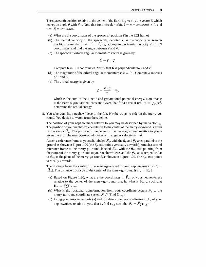
The spacecraft position relative to the center of the Earth is given by the vector~r, whichmakes an angleθ with ~xG. Note that for a circular orbit,θ = n = constant > 0, andr = |~r| = constant.
(a) What are the coordinates of the spacecraft position~r in the ECI frame?
(b) The inertial velocity of the spacecraft, denoted~v, is the velocity as seen inthe ECI frame, that is~v = ~r = ~FT
G rG. Compute the inertial velocity~v in ECIcoordinates, and find the angle between~r and~v.
(c) The spacecraft orbital angular momentum vector is givenby
~h = ~r× ~v.
Compute~h in ECI coordinates. Verify that~h is perpendicular to~r and~v.
(d) The magnitude of the orbital angular momentum ish = |~h|. Computeh in termsof r andn.
(e) The orbital energy is given by
E =~v · ~v2
− µ
r,
which is the sum of the kinetic and gravitational potential energy. Note thatµis the Earth’s gravitational constant. Given that for a circular orbitn =
√
µ/r3,determine the orbital energy.
8. You take your little nephew/niece to the fair. He/she wants to ride on the merry-go-round. You decide to watch from the sideline.
The position of your nephew/niece relative to you may be described by the vector~rn.The position of your nephew/niece relative to the center of the merry-go-round is givenby the vector~Rn. The position of the center of the merry-go-round relative to you isgiven bye~rm. The merry-go-round rotates with angular velocityω = θ.
Attach a reference frame to yourself, labeledFy, with the~xy and~yy axes parallel to theground as shown in Figure 1.20 (the~zy axis points vertically upwards). Attach a secondreference frame to the merry-go-round, labeledFm, with the~xm axis pointing fromthe center of the merry-go-round to your nephew/niece, and the~ym axis perpendicularto~xm, in the plane of the merry-go-round, as shown in Figure 1.20.The~zm axis pointsvertically upwards.
The distance from the center of the merry-go-round to your nephew/niece isRn =|~Rn|. The distance from you to the center of the merry-go-round isrm = |~rm|.
(a) Based on Figure 1.20, what are the coordinates in~Fm of your nephew/niecerelative to the center of the merry-go-round, that is, what is Rn,m such that~Rn = ~FT
mRn,m?
(b) What is the rotational transformation from your coordinate systemFy to themerry-go-round coordinate systemFm? (FindCmy).
(c) Using your answers to parts (a) and (b), determine the coordinates inFy of yournephew/niece relative to you, that is, findrn,y such that~rn = ~FT
y rn,y.

10 Chapter 1 Exercises
You may take~rm = ~FTy
xm,yym,yzm,y
.
(d) Using your answer to part (c), determine the velocity of your nephew/niece asseen by you.
(e) Using your answer to part (a), determine the velocity of your nephew/niece asseen by another person on the merry-go-round.
9. This problem puts some numbers to question 7.
A spacecraft is in a circular equatorial orbit about the earth with altitude600 km. Youwill need the following information:Earth’s gravitational parameter:µ = 3.986× 10⁵ km3/s2.Earth’s radius:Re = 6378 km.(Note that altitude means height above the earth’s surface).
(a) Referring to part 7(a), what is the spacecraft position in ECI coordinates whenθ = 30o?
(b) Using 7(b), what is the spacecraft velocity as seen in theECI frame? Note thatθ = n =
√
µ/r3. Also, compute the orbital speed,v = |~v|.(c) Referring to 7(c), compute the spacecraft orbital angular momentum vector in
ECI coordinates.
(d) Referring to 7(e), compute the spacecraft orbital energy.
10. The orientation of a reference frameF2 is obtained from the reference frameF1 bya 2-3-1 Euler rotation sequence, with anglesθy, θz andθx. Specifically, frameF2 isobtained from frameF1 by:- A rotationθy about they-axisof frameF1,- A rotationθz about thez-axisof the intermediate frameFi,- A rotationθx about thex-axisof the transformed frameFt.
(a) Obtain the rotation matrixC21.
(b) Using the result in (a), obtain expressions for computing θx, θy andθz from therotation matrix.
(c) Where is the singularity of the 2-3-1 rotation sequence?What does this physicallymean?
(d) Given that frameF2 rotates with angular velocity~ω21 = ~FT2 ω21 relative to frame
F1, obtain the kinematical relationship betweenω21 and
θxθyθz
.
(e) Using the result in (d), what happens to the kinematical relationship if the anglesθx, θy andθz and ratesθx, θy andθz are very small? Hints: for a small angleθ,you can setsin θ ≈ θ andcos θ ≈ 1. For very small quantitiesa andb, you canneglect productsab.

Chapter 1 Exercises 11
11. The orientation of a reference frameF2 is obtained from the reference frameF1 bya 3-2-3 Euler rotation sequence, with anglesθ1, θ2 andθ3. Specifically, frameF2 isobtained from frameF1 by:- A rotationθ1 about thez-axisof frameF1,- A rotationθ2 about they-axisof the intermediate frameFi,- A rotationθ3 about thez-axisof the transformed frameFt.
(a) Obtain the rotation matrixC21.(b) Given that frameF2 rotates with angular velocity~ω21 = ~FT
2 ω21 relative to frame
F1, obtain the kinematical relationship betweenω21 and
θ1θ2θ3
.
(c) Invert the result in part (b) to obtain
θ1θ2θ3
as a function ofω21. Hint: For a
general block lower triangular matrix,[
A 0B C
]−1
=
[
A−1 0−C−1BA−1 C−1
]
.
(d) Where is the singularity of the 3-2-3 rotation sequence?What does this physicallymean?
12. Hooke’s joint is shown in Figure 1.21. It can be used in machinery to transmit rotationalpower when the axis of rotation needs to change slightly. As shown in Figure 1.21,Hooke’s joint consists of three components. An input shaft,an output shaft and a crossin the middle. The cross is connected to each shaft such one axis of the cross rotateswith the input shaft and the other axis of the cross rotates with the output shaft.
It can be seen from Figure 1.21 that the output shaft has an angle α with respect tothe input shaft, with|α| < 90o. We define two fixed (non-rotating) reference framesFi andFo, such that
• thex-axis ofFi is parallel to the axis of rotation of the input shaft,• thex-axis ofFo is parallel to the axis of rotation of the output shaft and• they-axes ofFi andFo coincide.
The rotational angle of the input shaft is labeledθi and the rotational angle of theoutput shaft is labeledθo.
We also attach a reference frameFc to the cross, as shown in Figures 1.21 and 1.22.
(a) Write down the rotation matrixCoi corresponding to the transformation fromFitoFo.
(b) We further attach reference framesF2 andF3 to the input and output shaftsrespectively, as shown in Figures 1.23 and 1.24. Write down the rotation matricesC2i andC3o. You may assume that~Fi = ~F2 when θi = 0 and that ~Fo = ~F3
whenθo = 0.

12 Chapter 1 Exercises
(c) What is the rotational transformation fromF3 to Fc? Write down thecorresponding rotation matrixCc3.
(d) By considering the rotational transformationsFc → F3 → Fo andFc → F2 →Fi → Fo, obtain two expressions for thez-axis ofFc in Fo coordinates. Hint:You may use the fact that~zc = ~z2.
(e) Using the expressions obtained in part (d), show that theinput and outputrotational angles are related by
sin θo =sin θi
(
1− sin2 α cos2 θi)
1
2
,
cos θo =cosα cos θi
(
1− sin2 α cos2 θi)
1
2
.
13. Show that for any unit column matrixa ∈ R3 with aTa = 1,
a×a×a× = −a×.
14. Making use of the scalar-triple product and vector-triple product identities, show that(
~a× ~b)
·(
~c× ~d)
= (~a · ~c)(
~b · ~d)
−(
~a · ~d)(
~b · ~c)
.
15. Consider the axis-angle parameters,a andφ.
(a) Starting with the expression for the rotation matrix given in (1.26) in the book,obtain an approximate expression for the rotation matrix when the angle ofrotationφ is very small. The quantityφ = aφ will be useful (this is sometimescalled therotation vector).
(b) Show that the axis-angle parameters(a3, φ3) equivalent to successive rotations(a1, φ1) followed by(a2, φ2) are given by
a3 =1
sin(φ3/2)
[
sinφ12
cosφ22a1 + sin
φ22
cosφ12a2 + sin
φ12
sinφ22a×1 a2
]
,
cosφ32
= cosφ12
cosφ22
− sinφ12
sinφ22aT1 a2.
(c) Show that their kinematical equations are given by
a =1
2
(
a× − 1
tan(φ/2)a×a×
)
ω,
φ = aTω.
(d) Show that the inverse kinematics are given by
ω =(
sinφ1− (1− cosφ)a×)
a+ aφ.
What does this reduce to when the rotation is about a fixed axis?

Chapter 1 Exercises 13
(e) Is there a singularity associated with these parameters?
(f) Starting with the inverse kinematics obtained in part (d), obtain an approximateexpression forω when the angle of rotationφ is very small. The quantityφ = aφwill again be useful.
16. Consider the rotation vectorφ = aφ, introduced in Question 15.
(a) Show that the rotation matrix associated withφ is given by
C = 1+(1− cosφ)
φ2φ×φ× − sinφ
φφ×,
whereφ = ‖φ‖.
(b) Show that the kinematical equations for the rotation vector are
φ =
(
1+φ×
2+
1
φ2
[
1− φ/2
tan(φ/2)
]
φ×φ
×
)
ω.
(c) Show that the inverse kinematics are given by
ω =
(
1− (1− cosφ)
φ2φ× +
(φ− sinφ)
φ3φ×φ×
)
φ.
(d) Where is the singularity associated with these parameters? Careful, it is not atφ = 0.
17. Consider the following parameterization of the rotation matrix
p = a tanφ
2.
These are called the Euler-Rodrigues parameters.
(a) Show that the rotation matrix associated withp is given by
C =(1− pTp)1+ 2ppT − 2p×
1 + pTp.
(b) Starting with the expression for the rotation matrix obtained in part (a), obtain anapproximate expression for the rotation matrix whenp is very small.
(c) Show that the Euler-Rodriguez parameters may be obtained from a rotationmatrix by
p =1
1 + C11 + C22 + C33
C23 − C32
C31 − C13
C12 − C21
.
(d) Show that the rotationp3 equivalent to successive rotationsp1 followed byp2 isgiven by
p3 =p1 + p2 + p×
1 p2
1− pT1 p2.

14 Chapter 1 Exercises
(e) Show that the kinematical equations for the Euler-Rodrigues parameters are
p =1
2(1+ ppT + p×)ω.
(f) Show that the inverse kinematics are given by
ω =2(1− p×)p
1 + pTp.
(g) Starting with inverse kinematics obtained in part (f), obtain an approximateexpression forω whenp andp are very small.
(h) Where is the singularity associated with these parameters?
18. Consider the following parameterization of the rotation matrix
σ = a tanφ
4.
These are called the modified Euler-Rodrigues parameters.
(a) Show that the rotation matrix associated withσ is given by
C = 1+8σ×σ× − 4(1− σTσ)σ×
(1 + σTσ)2.
(b) Starting with the expression for the rotation matrix obtained in part (a), obtain anapproximate expression for the rotation matrix whenσ is very small.
(c) Setting s = C11 + C22 + C33, show that the modified Euler-Rodriguesparameters may be obtained from a rotation matrix by
σ =1
1 + s+ 2√1 + s
C23 − C32
C31 − C13
C12 − C21
,
when‖σ‖ < 1,
σ =1
1 + s− 2√1 + s
C23 − C32
C31 − C13
C12 − C21
,
when‖σ‖ > 1, andσ = a (the principal axis of rotation) when‖σ‖ = 1.(d) Show that the rotationσ3 equivalent to successive rotationsσ1 followed byσ2
is given by
σ3 =(1 − σT2 σ2)σ1 + (1 − σT1 σ1)σ2 + 2σ×
1 σ2
1 + (σT1 σ1)2(σT2 σ2)2 − 2σT1 σ2.
(e) Show that the kinematical equations for the modified Euler-Rodrigues parametersare
σ =1
4
(
(1 − σTσ)1+ 2σσT + 2σ×)
ω.

Chapter 1 Exercises 15
(f) Show that the inverse kinematics are given by
ω =4
(1 + σTσ)2(
(1− σTσ)1+ 2σσT − 2σ×)
σ.
(g) Starting with inverse kinematics obtained in part (f), obtain an approximateexpression forω whenσ andσ are very small.
(h) Where is the singularity associated with these parameters? What are theadvantages of the modified Euler-Rodrigues parameters compared to the Euler-Rodrigues parameters (introduced in Question 17)?
19. In this question, we consider a reference frameF1 defined by three non-coplanar unitvectors,~11, ~12 and~13, which are not necessarily orthogonal. Note that we reservethe notation~x, ~y and~z for the basis vectors of orthogonal right-handed frames ofreference, which is why we do not use them here. Just as in Section 1.2 of the book,since the basis vectors,~11, ~12 and ~13 are non-coplanar, we may represent everyphysical vector~r as
~r = ~FT1 r1,
where
~F1 =
~11
~12
~13
,
is the vectrix containing the basis vectors defining frameF1, and
r1 =
r1,1r2,1r3,1
,
is the column matrix containing the coordinates of~r in frameF1. Note that for twophysical vectors~a = ~FT
1 a1 and~b = ~FT1 b1, it is easy to verify that
~a+ ~b = ~FT1 (a1 + b1),
and that for any scalarc,
c~a = ~FT1 (ca1).
(a) Show that for any two physical vectors~a = ~FT1 a1 and~b = ~FT
1 b1, the scalarproduct obeys
~a · ~b = aT1 W1b1,
where
W1 =
~11 · ~11~11 · ~12
~11 · ~13
~12 · ~11~12 · ~12
~12 · ~13
~13 · ~11~13 · ~12
~13 · ~13
.
Furthermore, verify that the matrixW1 is symmetric and positive definite.
16 Chapter 1 Exercises
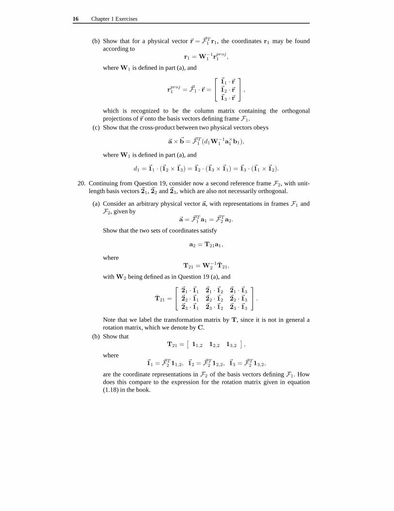
(b) Show that for a physical vector~r = ~FT1 r1, the coordinatesr1 may be found
according tor1 = W−1
1 rproj1 ,
whereW1 is defined in part (a), and
rproj1 = ~F1 ·~r =
~11 ·~r~12 ·~r~13 ·~r
,
which is recognized to be the column matrix containing the orthogonalprojections of~r onto the basis vectors defining frameF1.
(c) Show that the cross-product between two physical vectors obeys
~a× ~b = ~FT1 (d1W
−11 a×1 b1),
whereW1 is defined in part (a), and
d1 = ~11 · (~12 × ~13) = ~12 · (~13 × ~11) = ~13 · (~11 × ~12).
20. Continuing from Question 19, consider now a second reference frameF2, with unit-length basis vectors~21, ~22 and~23, which are also not necessarily orthogonal.
(a) Consider an arbitrary physical vector~a, with representations in framesF1 andF2, given by
~a = ~FT1 a1 = ~FT
2 a2.
Show that the two sets of coordinates satisfy
a2 = T21a1,
whereT21 = W−1
2 T21,
with W2 being defined as in Question 19 (a), and
T21 =
~21 · ~11~21 · ~12
~21 · ~13
~22 · ~11~22 · ~12
~22 · ~13
~23 · ~11~23 · ~12
~23 · ~13
.
Note that we label the transformation matrix byT, since it is not in general arotation matrix, which we denote byC.
(b) Show thatT21 =
[
11,2 12,2 13,2
]
,
where~11 = ~FT
2 11,2, ~12 = ~FT2 12,2, ~13 = ~FT
2 13,2,
are the coordinate representations inF2 of the basis vectors definingF1. Howdoes this compare to the expression for the rotation matrix given in equation(1.18) in the book.

Chapter 1 Exercises 17
(c) Noting thatT21 = TT12, show that
T21 = W−12 TT
12W1.
(d) Leta2 = T21a1. Show that
a×2 =
(
d1d2
)
TT12a
×1 T12.
whered1 andd2 are defined as in Question 19 (c). How does this compare toequation (1.21) in the book?
21. Define the derivative of a physical vector~r = ~FT1 r1 as seen in a not-necessarily
orthogonal frameF1 by·1
~r∆= ~FT
1 r1.
Show that the rules for differentiation obtained in Section1.4 of the book hold in thiscase also. Note that we assume that the basis vectors ofF1 are fixed relative to eachother.
22. Consider the framesF1 andF2 from question 19. Define right-handed orthogonalframesF1o andF2o such thatF1 is fixed inF1o, andF2 is fixed inF2o. Define theangular velocity~ω21 of frameF2 relative to frameF1 by
~ω21 = ~ω2o,1o.
Note that this is well defined, since any choice of orthogonalright-handed framesF1o andF2o would lead to the same angular velocity vector. Indeed, letF1o′ andF2o′ be another pair of right-handed orthogonal reference frames such thatF1 isfixed in F1o′ , andF2 is fixed inF2o′ . Then,~ω1o′,1o = ~ω2o′,2o = ~0, which leads to~ω2o,1o = ~ω2o′,1o′ .
(a) Consider~r = ~FT1 r1 = ~FT
1or1o. Show that
·1
~r=·1o
~r .
(b) Making use of the Transport Theorem for right-handed orthogonal referenceframes (equation (1.52) in the book), and part (a), show thatthe TransportTheorem also holds for non-orthogonal reference frames. That is, show
·1
~r=·2
~r +~ω21 ×~r.
(c) Let ~ω21 = ~FT2 ω21. Show that the rotational kinematics are given by
T21 = −d2W−12 ω×
21T21,
whereT21 was introduced in Question 20 (a), andd2, W2 were defined inQuestion 19. How does this compare to Poisson’s equation (equation (1.55) inthe book)?
18 Chapter 1 Exercises
~c
~b
~ah1
A1
Side 1
Side 2
Side 3
Side 4
Side 5
Side 6
Figure 1.1 Parallelepiped defined by~a, ~b and~c
~c
~b
θ
Figure 1.2 Parallelogram defined by~b and~c
~c
~b
~a~n
Figure 1.3 Unit normal vector to~b and~c
Chapter 1 Exercises 19
~c
~b
~a
Side 2
Side 5
h2
A2
Figure 1.4 Parallelepiped defined by~a, ~b and~c
~c
~b
~ah1
A1
Side 1Side 2
Side 3
Side 4
Side 5
Side 6
Figure 1.5 Parallelepiped defined by~a, ~b and~c
~c
~b
~a~b× ~c
~a⊥
Figure 1.6 Question 3 scenario

20 Chapter 1 Exercises
~c
~b
θ
~c‖b
~c⊥b
Figure 1.7 Components of~c relative to~b
~b× ~c
~a⊥
~a⊥rot
90o
Figure 1.8 Rotation of~a⊥
90o
~n2
~n1
Figure 1.9 Rotation of~n1 and~n2

Chapter 1 Exercises 21
~x
~y
~z
Figure 1.10 Left-handed reference frame
Base
Joint 1
Joint 2
Joint 3
Joint 4Joint 5
Link 1
Link 2
Link 3Link 4
Link 5
Hand
~r12
~r23
~r34~r45
~r5H
~rH
Figure 1.11 5-link robotic manipulator
Base attached to room
~xr
~yr
~zr
Figure 1.12 Room Frame Definition

22 Chapter 1 Exercises
Joint i
Joint i+1
Link i
~xi
~yi
~zi
Figure 1.13 Robot link frame definition
~xr
~yr, ~y1
~zr~z1
~x1
θ1
θ1
Figure 1.14 Joint 1 rotation
Joint 1
Joint 2Link 1
~x1~y1
~z1
Link 2
~x1, ~x2 ~y1
~z1
~z2
~y2
θ2
θ2
Figure 1.15 Joint 2 rotation

Chapter 1 Exercises 23
~xG
~yG
~zG,~zF
Equator
ωearth
~xF
~yF
θGMT
Figure 1.16 ECI and ECEF frame definitions
~zF
~yFδ
λ
~xF
~xT
~zT
~yT
Figure 1.17 Topocentric frame definition
~zF
~xF
~yF
Satellite
Ground Station
δ
λ
~Rs
~r~ρ
Figure 1.18 Ground station and satellite geometry

24 Chapter 1 Exercises
Spacecraft
Earth
~xG
~yG
Orbit
~r
~v
θ
Figure 1.19 Circular Equatorial Orbit
~xG~ym
~Rn
~rn
~rm
ω
θ
Merry-go-round
Nephew/Niece
You
~yy
~xy
Figure 1.20 Merry-go-round scenario
α
~zc ~yc
~zi ~yi
~xi
θi
Fi ~zo~yo
~xo
Fo
θo
Figure 1.21 Hooke’s joint

Chapter 1 Exercises 25
~zc ~yc
~xcFc
Figure 1.22 Hooke’s joint cross
~y2
~x2
~z2
F2
Figure 1.23 Hooke’s joint input shaft
~z2
~y2
~x2
F2
Figure 1.24 Hooke’s joint output shaft


2Chapter 2 Exercises
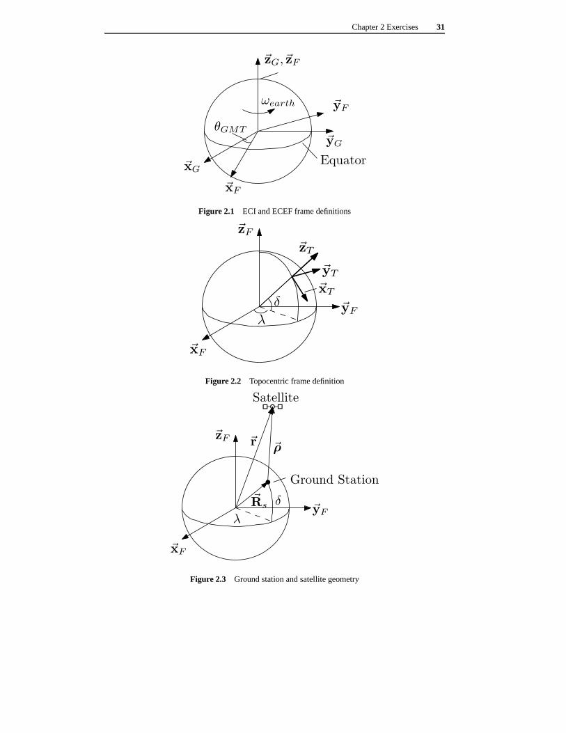
1. This question makes use of the Earth-Centered-Inertial (ECI) FG, Earth-Centered-Earth-Fixed (ECEF)FF and TopocentricFT reference frames. The figures definingthe frames are reproduced in Figures 2.1 and 2.2. Figure 2.3 shows the location ofa ground station, which is tracking a satellite. For Earth-Orbiting satellites, the ECIframe can be considered to be inertial.
The position of the satellite relative to the center of the earth is given by the vector~r. The position of the satellite relative to the ground station is given by the vector~ρ.The position of the ground station relative to the center of the earth is given by thevector ~Rs. The Topocentric frame has it’s origin at the ground stationlocation. Theangular velocity of the Earth (angular velocity of frameFF relative toFG) is given bythe vector~ωFG, and is constant as seen in the ECI and ECEF frames.
The mass of the satellite ism, and the sum of all external forces acting on the satelliteis given by the vector~F.
(a) Show that the vector equation of motion of the satellite as seen by an observer atthe ground station (as seen inFT ) is given by
m
~ρ= −2m~ωFG×
~ρ −m~ωFG × (~ωFG × ~Rs)−m~ωFG × (~ωFG × ~ρ) + ~F,
where() denotes time differentiation as seen in frameFT .
(b) Given the coordinates of the~ρ in F , the coordinates of~ωFG, ~Rs anFF , and thecoordinates of~F in FG, that is, given
~ρ = ~FTT ρ, ~ωFG = ~FT
F ωFG,~Rs = ~FT
FRs, ~F = ~FTGF,
show that in topocentric coordinates, the equation of motion obtained in part (a)is given by
mρ = −2mCTFω×FGC
TTF ρ−mCTFω
×FGω
×FGRs −mCTFω
×FGω
×FGC
TTFρ+CTGF,
whereCTF is the transformation fromFF to FT coordinates andCTG is thetransformation fromFG toFT coordinates.
Spacecraft Dynamics and Control - An Introduction,Anton H.J. de Ruiter, Christopher J. Damaren and James R. Forbes,c© 2013 John Wiley & Sons, Ltd. Published 2013 by John Wiley & Sons, Ltd.
Companion Website: http://www.wiley.com/go/deruiter/spacecraft
28 Chapter 2 Exercises
2. Consider the moment of inertia matrix
J =
Jxx Jxy JxzJxy Jyy JyzJxz Jyz Jzz
.
Show that for any three-dimensional body
Jxx − Jyy + Jzz > 0
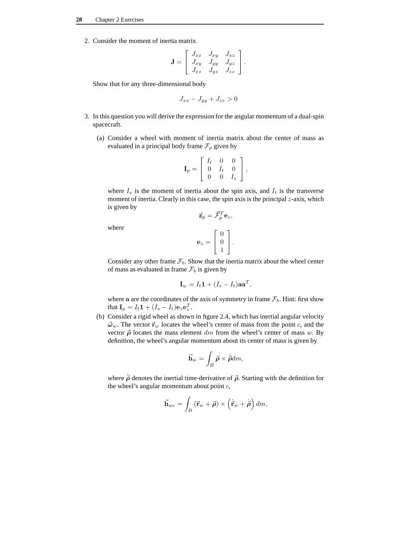
3. In this question you will derive the expression for the angular momentum of a dual-spinspacecraft.
(a) Consider a wheel with moment of inertia matrix about the center of mass asevaluated in a principal body frameFp given by
Ip =
It 0 00 It 00 0 Is
,
whereIs is the moment of inertia about the spin axis, andIt is the transversemoment of inertia. Clearly in this case, the spin axis is the principalz-axis, whichis given by
~zp = ~FTp ez,
where
ez =
001
.
Consider any other frameFb. Show that the inertia matrix about the wheel centerof mass as evaluated in frameFb is given by
Iw = It1+ (Is − It)aaT ,
wherea are the coordinates of the axis of symmetry in frameFb. Hint: first showthatIp = It1+ (Is − It)eze
Tz .
(b) Consider a rigid wheel as shown in figure 2.4, which has inertial angular velocity~ωw. The vector~rw locates the wheel’s center of mass from the pointc, and thevector~ρ locates the mass elementdm from the wheel’s center of massw. Bydefinition, the wheel’s angular momentum about its center ofmass is given by
~hw =
∫
B
~ρ× ~ρdm,
where~ρ denotes the inertial time-derivative of~ρ. Starting with the definition forthe wheel’s angular momentum about pointc,
~hwc =
∫
B
(~rw + ~ρ)×(
~rw + ~ρ)
dm,

Chapter 2 Exercises 29
show that the wheel’s angular momentum about the pointc is given by
~hwc = mw~rw × ~rw + ~hw,
wheremw is the total mass of the wheel.
(c) Consider the dual-spin spacecraft as shown in figure 2.5.We divide the spacecraftinto two parts: the wheel (labeledW ), and the rest of the spacecraft, called theplatform (labeledP ). The pointc denotes the center of mass of the spacecraft(the combined platform and wheel). The vector~rw = ~FT
b rw locates the center ofmass of the wheel from the center of mass of the spacecraft. Let Fb be a body-fixed reference frame attached to the platform. The platformhas inertial angularvelocity ~ω = ~FT
b ω. The wheel has angular velocity~ωs = ωs ~FTb a relative to the
platform, where~a = ~FTb a is the wheel spin axis, andωs is the wheel spin-rate
relative to the platform. The wheel moment of inertia about the spin axis is labeledIs, and the wheel transverse moment of inertia is labeledIt.
Show that the wheel angular momentum vector about the wheel center of mass isgiven by
~hw = ~FTb [Iwω + hsa] ,
wherehs = Isωs is the wheel relative angular momentum, and
Iw = It1+ (Is − It)aaT .
(d) Given that the wheel has massmw, use the result in part (b) to show that thewheel angular momentum about the spacecraft center of massc is given by
~hwc = ~FTb [Jwcω + hsa] ,
whereJwc = Iw −mwr×wr
×w is the wheel moment of inertia matrix about the
spacecraft center of massc evaluated inFb.(e) Finally, show that the total angular momentum of the spacecraft (platform plus
wheel) about the spacecraft center of mass is given by
~hc = ~FTb [Iω + hsa] ,
whereI = Jpc + Jwc is the moment of inertia matrix of the spacecraft about thecenter of massc, andJpc is the platform moment of inertia about the spacecraftcenter of massc.
4. Consider again the dual-spin satellite from Question 3, shown in Figure 2.5. Let~vc = ~FT
b vc be the inertial velocity of pointc, which as we recall is the center of massof the spacecraft (combined platform and wheel).
(a) Show that the kinetic energy of the wheel is given by
Tw =1
2mwv
2c + vTc ω
×(mwrw) +1
2ωTJwcω + Isωsa
Tω +1
2Isω
2s ,
wherevc = ‖vc‖, and all other quantities are defined in Question 3.

30 Chapter 2 Exercises
(b) Show that the platform kinetic energy is given by
Tp =1
2mpv
2c + vTc ω
×cp +1
2ωTJpcω,
wherecp =∫
pρdm is the platform first moment of mass about pointc, andmp
is the total platform mass.
(c) Combining the results from parts (a) and (b), show that the total spacecraft kineticenergy is given by
T = Tt + Tr,
whereTt =
1
2mv2c ,
is the spacecraft translational kinetic energy, andm = mp +mw is the totalspacecraft mass, and
Tr =1
2ωT Iω + Isωsa
Tω +1
2Isω
2s ,
is the spacecraft rotational kinetic energy. Hint:mprw is the first moment of massof the wheel about the pointc.
Chapter 2 Exercises 31
~xG
~yG
~zG,~zF
Equator
ωearth
~xF
~yF
θGMT
Figure 2.1 ECI and ECEF frame definitions
~zF
~yFδ
λ
~xF
~xT
~zT
~yT
Figure 2.2 Topocentric frame definition
~zF
~xF
~yF
Satellite
Ground Station
δ
λ
~Rs
~r~ρ
Figure 2.3 Ground station and satellite geometry

32 Chapter 2 Exercises
c
~rw
dm
~ρ
Figure 2.4 Wheel
c
~rwFb
W
P
~a
Figure 2.5 Dual-spin satellite

3Chapter 3 Exercises
For some of the following questions, you will need the Earth’s gravitational constant
µ⊕ = 3.986× 10⁵ km3/s2,
the Sun’s gravitational constant
µ⊙ = 1.3271244× 10¹¹ km3/s2,
and
1 AU = 1.4959787× 10⁸ km.
1. A spacecraft is observed with inertial position and velocity vectors relative to the centerof the Earth, given in ECI coordinates by
~r = ~FTG =
1670.63191670.63196491.2735
km, ~v = ~FTG =
−5.3429−5.34293.3788
km/s.
The Earth’s gravitational constant is given byµ⊕ = 3.986× 10⁵ km3/s2.
(a) Compute the orbital angular momentum vector~h in ECI coordinates.
(b) Compute the orbital energy,E . What type of orbit is it?
(c) Compute the eccentricity vector~e in ECI coordinates.
(d) Compute the eccentricity,e and the semi-latus rectump.
(e) Compute the true anomaly,θ, noting thatθ is measured positive from~e as aright-hand rotation about~h.
(f) Compute the radius at periapsisrmin.
(g) Compute the spacecraft position vector at periapsis in ECI coordinates.
(h) Compute the orbital speed at periapsis.
(i) Compute the angle,i, between the orbital plane and the Earth’s equatorial plane,noting that~h is a vector normal to the orbit, and~zG is a vector normal to theequator.
Spacecraft Dynamics and Control - An Introduction,Anton H.J. de Ruiter, Christopher J. Damaren and James R. Forbes,c© 2013 John Wiley & Sons, Ltd. Published 2013 by John Wiley & Sons, Ltd.
Companion Website: http://www.wiley.com/go/deruiter/spacecraft

34 Chapter 3 Exercises
2. A geosynchronousorbit has semi-major axis and eccentricity:
a = 42241.08007 km,e = 0.
(a) Compute the orbital period in hours. What can you conclude about a satellite ina geosynchronous orbit?
(b) A geostationaryorbit is a geosynchronous orbit with zero inclinationi = 0.What is the plane of the orbit? What can you conclude about a satellite in ageosynchronous orbit in relation to an observer on the ground?
3. Halley’s comet last passed perihelion on February 9, 1986. It has a semimajor axisof 17.9564 AU and eccentricitye = 0.967298 (one AU is the semimajor axis of theearth’s orbit around the sun). Predict the date of its next return.
4. A satellite is in a geocentric Keplerian (two-body) orbitwith a period of 270 minutesand eccentricitye = 0.5. It has passed perigee and is now at a point in which the orbitalradius is the same as the semi-latus rectum. How much time (inminutes) has elapsedsince perigee passage?
5. An earth-orbiting spacecraft has classical orbital elements
a = 8000 km,e = 0.1,i = 45o,ω = 0o,Ω = 90o.
The spacecraft currently has true anomalyθ = 30o.
(a) Determine the spacecraft position and velocity vectorsin perifocal coordinates.
(b) Determine the transformation from perifocal to ECI coordinatesCGp.
(c) Determine the spacecraft position and velocity vectorsin ECI coordinates.
6. At timet = 0, the position and velocity vectors for an earth-orbiting satellite are givenin ECI coordinates as:
~r = ~FTG
−3718.81602.96517.7
km,
~v = ~FTG
−4.8991−5.4428−0.6659
km/s.
(a) Find the classical orbital elements
(b) Thirty minutes later, what are~r and~v? (Express your answers in ECI coordinates)
7. An earth-orbiting satellite has orbital radius and speedat perigee
rp = 7000 km, vp = 8 km/s.
Chapter 3 Exercises 35
(a) Determine the orbital period,T in minutes.(b) Determine the orbital speed twenty minutes after perigee passage.
8. At timet = 0, the position and velocity vectors for an earth-orbiting satellite are givenin ECI coordinates as:
~r = ~FTG
1.703× 10⁵
0.0426× 10⁵
0.638× 10⁵
km,
~v = ~FTG
0.09721.2711.465
km/s.
(a) Find the classical orbital elements(b) Twenty minutes later, what are~r and ~v? (Express your answers in ECI
coordinates)
9. By starting with the polar solution for an orbit, and the equation for the orbital angularmomentum, show that the time-of-flight equation for a parabolic orbit is given by
6
√
µ
p3(t− t0) = 3 tan
θ
2+ tan3
θ
2,
wheret− t0 denotes the time since periapsis passage.
10. In this question you are going to derive the time-of-flight equation for a hyperbolicorbit.
First, we need to discuss hyperbolic functions. The hyperbolic sine, cosine and tangentare defined as
sinhx∆=ex − e−x
2and coshx
∆=ex + e−x
2, tanhx
∆=
sinhx
coshx,
respectively. From these definitions, the following property can readily be shown.
cosh2 x− sinh2 x = 1.
The derivatives are readily obtained as
d
dxsinhx = coshx,
d
dxcoshx = sinhx,
d
dxtanhx =
1
cosh2 x.
Similar to the trigonometric functions, the following “double-angle” formulae can alsoreadily be found
coshx = 2 cosh2x
2− 1, sinhx = 2 sinh
x
2cosh
x
2.
Consider the hyperbola satisfying
x2
a2− y2
b2= 1, with a < 0, b < 0.
36 Chapter 3 Exercises
As shown in figure 3.1, the hyperbola has two branches. The left-hand branch of thehyperbola can be represented parametrically by
x = a coshP, y = −b sinhP
We now consider a hyperbolic orbit with eccentricitye > 1, a < 0 andb = a√e2 − 1.
Since a hyperbolic orbit corresponds to the left-hand branch of a hyperbola, we canrepresent thex andy components of the orbital position in perifocal coordinates by
xp = −ae+ a coshH, yp = −b sinhH,
where we callH the “hyperbolic eccentric anomaly”.
(a) Show that the orbital radius satisfies
r = a(1− e coshH).
(b) Show that
cos θ =a [coshH − e]
r,
and
sin θ =−a
√e2 − 1 sinhH
r.
(c) By applying trigonometric and hyperbolic double angle formulae to the results inpart (b), show that
cos2θ
2=
−a(e− 1) cosh2 H2r
,
and
sinθ
2cos
θ
2=
−a√e2 − 1 sinh H
2 cosh H2
r.
(d) Using the results from part (c), show that the true anomaly and the hyperboliceccentric anomaly are related by
tanθ
2=
√
e+ 1
e− 1tanh
H
2.
(e) By differentiating the result in part (d), and making useof the first result in part(c), show that
dθ
dH= −a
√e2 − 1
r.
(f) Let t0 be the time of periapsis passage. Evaluate the integral∫ t
t0
hdτ =
∫ θ
0
r2dθ
to obtain the hyperbolic form of Kepler’s equation
e sinhH −H =
√
µ
−a3 (t− t0) .

Chapter 3 Exercises 37
11. The inertial position and velocity of a spacecraft over the Earth are observed in the ECIframe to be
~r = ~FTG
900090000
km, ~v = ~FTG
007
km/s.
Calculate:
(a) The angular momentum vector~h.
(b) The inclinationi,
(c) the right ascension of the ascending node,Ω.
12. Consider the circle of radiusa as shown in figure 3.2. The wedge bounded by a radiuswith angleE from thex-axis and thex-axis itself may be divided into two parts: atriangular part with areaAt and the remaining part with areaAo. Therefore, the areaof the wedge is given by
Aw = At +Ao.
(a) Show that the areaAo is given by
Ao =1
2a2 [E − sinE cosE] .
(b) Referring to figure 3.3, it can be seen that the area of an orbit swept out by theradius vector from periapsis at timet0 to the current timet, can be divided intotwo parts: a triangular part with areaA2 and the remaining part with areaA1.Show that
A2 =ab
2[sinE cosE − e sinE] ,
whereb is the semi-minor axis, ande is the eccentricity.
(c) Given thatA1 = (b/a)A0, whereA0 was found in part (a), show that the areaswept out by the radius vector is given by
A(t) =ab
2[E − e sinE] .
(d) Using the result from part (c), make use of Kepler’s second law to derive Kepler’sequation.
13. A spacecraft is in a geocentric Keplerian orbit. It has passed perigee, and is currently ata position where the orbital radius is equal to the semi-latus rectum. The current orbitalradius and speed are
r = 7000 km, v = 7.5555 km/s.
How much time has elapsed since perigee passage?

38 Chapter 3 Exercises
x
y
Figure 3.1 Left and right branches of a hyperbola
x
y
a
E
At
Ao
Figure 3.2 Segment of bounding circle
x
y
a
E
r
θ
A1
A2
yp
ae xp
periapsis
Figure 3.3 Area swept out by orbital radius

4Chapter 4 Exercises
For some of the following questions, you will need the Earth’s gravitational constant
µ⊕ = 3.986× 10⁵ km3/s2,
the Sun’s gravitational constant
µ⊙ = 1.3271244× 10¹¹ km3/s2,
Earth’s heliocentric orbital radius
R⊕ = 1.49598023× 10⁸ km,
and Mars’ heliocentric orbital radius
RMars = 2.27939186× 10⁸ km.
1. Radar observations have provided the following successive position vectors of anobject orbiting the earth:
~r1 = ~FTG
700000
km,
~r2 = ~FTG
5846.85846.8
0
km,
~r3 = ~FTG
0147000
km.
(a) Determine whether the orbit is elliptic, parabolic or hyperbolic.
(b) Determine the radius at perigee.
(c) Determine the orbital speed at perigee.
Spacecraft Dynamics and Control - An Introduction,Anton H.J. de Ruiter, Christopher J. Damaren and James R. Forbes,c© 2013 John Wiley & Sons, Ltd. Published 2013 by John Wiley & Sons, Ltd.
Companion Website: http://www.wiley.com/go/deruiter/spacecraft

40 Chapter 4 Exercises
2. Radar observations have provided the following successive position vectors of anobject orbiting the earth:
~r1 = ~FTG
3467.33467.34903.5
km,
~r2 = ~FTG
00
7425.0
km,
The time between observations ist2 − t1 = 740.6 seconds. You may assume that theobject is in an elliptical orbit. For simplicity, you may take η = ηH as the sector-triangle area ratio.
(a) Determine the orbital period.(b) Determine the eccentricity of the orbit.
3. It is desired to perform an interplanetary transfer from Earth to Mars. It is determinedthat a Hohmann transfer requires too much time. Assume that the Earth and Mars bothpossess coplanar circular orbits. At timet = 0, the Earth has true anomalyθE(0) = 0,and Mars has true anomalyθM (0) = 30o. The spacecraft is desired to arrive at Marswhen Mars has a true anomalyθM = 45o. See Figure 4.1.
(a) Determine the time of flight of the transfer in days.(b) Determine the required heliocentric velocity vector for the spacecraft upon
departing the Earth’s sphere of influence. Use the coordinate system shown inFigure 4.1. You may takeη = ηH for the sector to triangle area ratio of thetransfer orbit.
4. Radar observations have provided the following successive position vectors of anobject orbiting the earth:
~r1 = ~FTG
−1568.39984895.65164570.7746
km,
~r2 = ~FTG
−3090.78663963.61074988.2121
km,
~r3 = ~FTG
−5431.07551739.93145070.6676
km.
Determine the semi-major axis, eccentricity and radius of perigee of the orbit.
5. Suppose that you are an astronaut onboard the International Space Station. You receivea radio message from Canadian Space Surveillance (CSS) thata previously undetectedasteroid is on a collision course with the Earth, and will likely impact somewhere nearOttawa. You are asked to fire a missile (which is kept onboard for such emergencies)

Chapter 4 Exercises 41
at the asteroid, which will break it into pieces small enoughto burn up upon entry intothe atmosphere. CSS informs you that the last point on the trajectory of the asteroidthat such an intercept is possible has ECI coordinates
~r2 = ~FTG
−2102.02476528.324286941.38176
km,
which is where the asteroid will be in precisely 12 minutes time. It will take you 2minutes to prepare the missile, at which time your location in ECI coordinates will be
~r1 = ~FTG
1668.390973624.995495163.39798
km.
What inertial velocity vector should the missile have upon being fired, in order to inter-cept the asteroid at~r2? Express your result in ECI coordinates.
Note: Upon firing, the missile has an impulsive (instantaneous) thrust to give it therequired velocity, after which it is in free orbital flight until intercept with the target.
6. Radar observations have provided the following successive position vectors of anobject orbiting the earth:
~r1 = ~FTG
1955.29484646.01215227.4178
km,
~r2 = ~FTG
107.88483469.94556531.6767
km,
~r3 = ~FTG
−2316.97371373.06327168.8558
km.
(a) Determine the position vector at perigee~rp in ECI coordinates.
(b) Determine the velocity vector at perigee~vp in ECI coordinates.
(c) Determine the time since perigee passaget2 − t0 for ~r2.
7. Verify the velocity vector at perigee obtained in 6(b), bysolving Lambert’s problemgiven~rp obtained in 6(a),~r2 and the time of flightt2 − t0 obtained in 6(c).

42 Chapter 4 Exercises
θM
SunEarth
Mars
~x
~y
Figure 4.1 Earth to Mars transfer

5Chapter 5 Exercises
For some of these questions, you will need the earth’s gravitational constant
µ⊕ = 3.986× 10⁵ km3/s2.
1. It is desired to change an initially elliptical orbit of semimajor axisa1 and eccentricitye1 to a larger elliptical orbit with semimajor axisa2 > a1, with the same radius ofperigeerp, but different argument of perigee (ω2 = ω1 +∆ω). Note that both orbitslie in the same plane. See Figure 5.1.
(a) Describe a double tangential maneuver that can accomplish this.
(b) Obtain an expression for the total∆v for the maneuver.
(c) Obtain an expression for the total time taken to execute the maneuver.
2. Two spacecraft are in the same geocentric elliptical orbit with semi-major axisa =10, 000 km and eccentricitye = 0.2, as shown in Figure 5.2. At the current time, theyhave true anomalies
θ1 = 45o andθ1 = 90o,
respectively. Determine the∆v spacecraft 1 must apply at periapsis if it is to catchspacecraft 2 with a single tangential maneuver.
3. A spacecraft is initially in a geocentric circular orbit of radiusrc = 7, 000 km. It isdesired to place the spacecraft in an elliptical orbit in thesame plane, of semi-majoraxisa = 20, 000 km and eccentricitye = 0.665.
Suggest a double-impulse maneuver to accomplish the transfer. Compute the total∆vand the time of flightTOF .
4. A spacecraft is launched into a circular orbit of radiusr1 = 8, 000 km with inclination,i = 45o. Compute the total∆v required to transfer the spacecraft into a geostationaryorbit (which has radiusr2 = 42, 221 km), assuming the inclination change isperformed at apoapsis of the transfer orbit.
5. A satellite leaves a circular parking orbit at inclination i and executes a Hohmanntransfer to a larger circular orbit in the equatorial plane.Part of the required inclinationchange∆i1 is performed during the first maneuver, and the remaining∆i2 = i−∆i1is done during the second maneuver.
Spacecraft Dynamics and Control - An Introduction,Anton H.J. de Ruiter, Christopher J. Damaren and James R. Forbes,c© 2013 John Wiley & Sons, Ltd. Published 2013 by John Wiley & Sons, Ltd.
Companion Website: http://www.wiley.com/go/deruiter/spacecraft

44 Chapter 5 Exercises
(a) If the speeds in the circular orbits arevc1 andvc2 respectively, and the perigeeand apogee speeds in the Hohmann transfer orbit arevp andva respectively, showthat the total∆v for both maneuvers is given by
∆v =[
v2c1 + v2p − 2vc1vp cos∆i1]
1
2 +[
v2c2 + v2a − 2vc2va cos (i−∆i1)]
1
2 .
(b) Obtain an expression ford∆v
d∆i1.
(c) Using the result from part (b), show that performing the entire inclination changeat apogee of the Hohmann transfer orbit (that is∆i1 = 0) is not optimal.
∆ω
rp
rp
Orbit 1
Orbit 2
Figure 5.1 Desired orbit change
θ1
θ2
Spacecraft 1
Spacecraft 2
Periapsis
Figure 5.2 Question 2 Scenario
6Chapter 6 Exercises
For the following exercises, you will need the Earth’s gravitational constant
µearth = 3.986× 10⁵ km3/s2,
the Sun’s gravitational constant
µsun = 1.3271244× 10¹¹ km3/s2,
Mars’ gravitational constant
µmars = 4.305× 10⁴ km3/s2,
Venus’ gravitational constant
µvenus = 3.257× 10¹⁴ m3/s2,
Jupiter’s gravitational constant,
µJup = 1.268× 10⁸ km3/s2,
Earth’s orbital radius about the sun
Rearth = 149.598023× 10⁶ km,
Mars’ orbital radius about the sun
Rmars = 227.939186× 10⁶ km,
Venus’ orbital radius about the sun
Rvenus = 108.208601× 10⁶ km,
Jupiter’s orbital radius about the sun,
RJup = 777.8× 10⁶ km,
and Saturn’s orbital radius about the sun,
RSat = 1486× 106 km.
Spacecraft Dynamics and Control - An Introduction,Anton H.J. de Ruiter, Christopher J. Damaren and James R. Forbes,c© 2013 John Wiley & Sons, Ltd. Published 2013 by John Wiley & Sons, Ltd.
Companion Website: http://www.wiley.com/go/deruiter/spacecraft

46 Chapter 6 Exercises
1. As part of a preliminary study for an exploration trip to Mars, it has been decided thata Hohmann transfer will be used to travel from the Earth to Mars. You may assumethat the orbits of the Earth and Mars are circular and lie in the same plane.
The spacecraft is initially in a circular parking orbit around the Earth of radiusrpark = 100, 000 km. It is desired to place the spacecraft in a circular orbit aroundMars of radiusrcapture = 50, 000 km.
(a) Compute the semi-major axis of the Hohmann transfer orbit.
(b) Compute the time-of-flight for the Hohmann transfer.
(c) Assuming that the Earth, Mars the Sun lie on the same line at t = 0, with Earthand Mars on opposite sides of the Sun, compute the timet in days of the requireddeparture from Earth.
(d) Compute the required hyperbolic excess speedv∞,dep upon exiting the Earth’ssphere of influence, and the hyperbolic excess speedv∞,arr upon entering Mars’sphere of influence.
(e) Determine the location and magnitude of the∆vdep required for Earth departure.
(f) Determine the required arrival hyperbola asymptote offset−b, and compute themagnitude of the∆varr required for Mars capture.
(g) Compute the total∆v for the trip.
2. As part of a preliminary study for an exploration trip to Venus, it has been decided thata Hohmann transfer will be used to travel from the Earth to Venus. You may assumethat the orbits of the Earth and Venus are circular and lie in the same plane.
The spacecraft is initially in a circular parking orbit around the Earth of radiusrpark = 100, 000 km. It is desired to place the spacecraft in a circular orbit aroundVenus of radiusrcapture = 50, 000 km.
(a) Compute the semi-major axis of the Hohmann transfer orbit.
(b) Compute the time-of-flight for the Hohmann transfer.
(c) Assuming that the Earth, Venus and the Sun lie along the same line att = 0 (onthe same side of the sun), compute the timet in days of the required departurefrom Earth.
(d) Compute the required hyperbolic excess speedv∞,dep upon exiting the Earth’ssphere of influence, and the hyperbolic excess speedv∞,arr upon entering Venus’sphere of influence.
(e) Determine the location and magnitude of the∆vdep required for Earth departure.
(f) Determine the required arrival hyperbola asymptote offset−b, and compute themagnitude of the∆varr required for Venus capture.
(g) Compute the total∆v for the trip.
3. Four incredibly lonely and homesick astronauts who got suckered into making a one-way trip to Mars, have found a resource (on Mars) that can be refined to create rocketfuel. However, this resource is limited, so they need to minimize the fuel required toget back to Earth. This necessitates a Hohmann transfer.

Chapter 6 Exercises 47
(a) The astronauts desperately want to return to Earth as soon as possible, so they donot want to miss the next launch window. Given that the current true anomaliesof Mars and the Earth areθMars = 45o and θEarth = 90o, how long do theastronauts have to make preparations?
(b) Assuming that they can make the next launch window, how long will it be untilthe astronauts are reunited with their families?
(c) The astronauts will initially launch into a circular parking orbit around Marsof radiusrpark = 30, 000 km, where they will perform a final check-out of alltheir systems before embarking on the return journey to the Earth. What is themagnitude of the∆v they must apply to get on the required escape hyperbola,and at what location relative to the velocity vector of Mars must it be applied?
4. It is desired to perform an interplanetary transfer from Mars to Jupiter. Assumethat Mars and Jupiter possess circular coplanar orbits and make other appropriatesimplifying assumptions.
(a) Calculate the required heliocentric velocities near Mars and near Jupiter.
(b) What is the required hyperbolic excess speed,v∞,dep, upon leaving Mars’ sphereof influence?
(c) If the approach distance at Jupiter is−b = 1, 050, 000 km, calculate theperijovian distance.
(d) Calculate the∆v to be applied at periapsis of the arrival hyperbola to capture thespacecraft into a circular orbit about Jupiter.
(e) If Mars and Jupiter are currently aligned on the oppositesides of the Sun, howmuch time until the next launch window?
5. A spacecraft on a Hohmann transfer from the Earth to Saturn, flies unexpectedlythrough the sphere of influence of Jupiter. The spacecraft approaches Jupiter on anentry asymptote offset of−b = 900, 000 km. Assume circular coplanar orbits forEarth, Jupiter and Saturn.
(a) What is the perijovian distance?
(b) What is the angle between the entrance and exit velocity vectors relative toJupiter?
(c) What will the spacecraft’s heliocentric energy gain be if the spacecraft passesbehind Jupiter?


7Chapter 7 Exercises
For the following questions, you will need the Earth’s gravitational constant
µ⊕ = 3.986× 10⁵ km3/s2,
J2 for the EarthJ2 = 0.001082,
and the equatorial radius of the Earth
Re = 6378.1363 km.
1. The perturbing gravitational potential for the Earth maysometimes be approximatedby
φp = −µr
[
J2
(
Rer
)2
P2(sin δ) + J3
(
Rer
)3
P3(sin δ)
]
whereRe is the equatorial radius,J2 andJ3 are zonal harmonic coefficients,P2(x) =32x
2 − 12 andP3(x) =
52x
3 − 32x are Legendre polynomials.
(a) Find the perturbing force per unit mass due to the above perturbing potential inthe spherical coordinate system (see Figure 7.1). The~∇ operator in sphericalcoordinates is given by
~∇(·) = ∂
∂r(·)~xs +
1
r cos δ
∂
∂λ(·)~ys +
1
r
∂
∂δ(·)~zs
Note that in Section 7.3.1 in the book, we obtained an expression for theacceleration due to theJ2 term directly in ECI coordinates. Strictly speaking, theEarth’s gravitational potential is fixed in a frame attachedto the Earth, namelythe ECEF frame. The reason the acceleration due toJ2 could be evaluateddirectly in the ECI frame is because it depends only on latitude (δ), and noton longitude (λ). Under the assumption that the ECI and ECEFz-axes areequal (~zG = ~zF ), the latitudeδ is the same in both ECI and ECEF frames,and the gravitational potential due toJ2 becomes identical in both frames. Inreality, there is a slight difference between~zG and ~zF . However, by makingthe approximation that~zG = ~zF , the analytical expressions for the effects ofJ2
Spacecraft Dynamics and Control - An Introduction,Anton H.J. de Ruiter, Christopher J. Damaren and James R. Forbes,c© 2013 John Wiley & Sons, Ltd. Published 2013 by John Wiley & Sons, Ltd.
Companion Website: http://www.wiley.com/go/deruiter/spacecraft

50 Chapter 7 Exercises
on the orbital elements in Section 7.3.4 in the book could be obtained. Strictlyspeaking, in the final equation for the acceleration due toJ2 (equation (7.40)),~zG should be replaced by~zF .
(b) Noting that the spherical coordinate frame is obtained from the ECEF frame bya rotationλ about the~zF axis, followed by a rotation−δ about the~ys axis, findthe perturbing force per unit mass due to theJ2 term in ECEF coordinates, andverify that this is the same as that presented in equation (7.40) in the book.
(c) By transforming the perturbing force per unit mass due totheJ3 term to ECEFcoordinates, show that the force per unit mass in terms of physical vectors is
~fp,J3=µJ3R
3e
2r5
[
5(~r · ~zF )r2
(
7(~r · ~zF )2
r2− 3
)
~r+ 3
(
1− 5(~r · ~zF )2
r2
)
~zF
]
2. Consider the perturbing potential for a non-spherical primary due to zonal terms only
φp(~r) = −µr
∞∑
n=2
Jn
(
Rer
)n
Pn(sin δ).
Show that the associated perturbing force/unit mass is given by
~fp =µ
r3
∞∑
n=2
Jn
(
Rer
)n
[((n+ 1)Pn(sin δ) + sin δP ′n(sin δ))~r− rP ′
n(sin δ)~zF ] ,
whereP ′n(x) = dPn(x)/dx and~zF is thez-axis of the ECEF frame.
3. A satellite is initially in a close-to-circular Earth orbit (very small eccentricity), asshown in Figure 7.2. However, a small disturbing force due tosolar radiation pressureacts continuously on the spacecraft in an inertially fixed direction, as shown. Assumethe solar radiation pressure force per unit mass is in the plane of the orbit, and hasmagnitudef .
(a) Express the tangential force componentfθ and the radial force componentfr interms off and the true anomaly,θ.
(b) Show that for the initially close-to-circular orbit, the evolutionary equations forthe semi-major axisa and the eccentricitye are (approximate by settinge = 0)
da
dt=
2a2√µaf cos θ
de
dt=
√
a
µf[
1 + cos2 θ]
(c) For a circular orbit, the angular rate is approximately constant, withθ =√
µa3
.Show that the evolutionary equations fora ande with respect to true anomaly,θare
da
dθ=
2f
n2cos θ
de
dθ=
f
an2
[
1 + cos2 θ]
wheren =√
µa3
is the orbital mean motion.

Chapter 7 Exercises 51
(d) As shown in Figure 7.3, only the lit portion of the orbit isaffected by the solarpressure force. The portion of the orbit shadowed by the Earth has a range of trueanomaliesθv ≤ θ ≤ 180o − θv as shown in the figure. Using the result in part(c), show that the changes ina ande over one orbit are given by
∆a = 0
∆e =f
an2
[
3(
θv +π
2
)
+sin(2θv)
2
]
4. (a) Show that for a sun-synchronous frozen orbit with semi-major axis,a, theeccentricitye is given by
e =
[
1−(
3J2R2e
2〈Ω〉ss
√
µ
5a7
)
1
2
]
1
2
,
where〈Ω〉ss = 360o/year.
(b) Compute the eccentricities and radii of perigee for a geocentric sun-synchronousfrozen orbits with semi-major axesa = 10, 000 km, a = 15, 000 km anda =20, 000 km. Conclude that there is a range of semi-major axes for which ageocentric sun-synchronous frozen orbit is possible.
(c) Sketch a plot of semi-major axis vs. radius of perigee fora geocentric sun-synchronous frozen orbit.
(d) Find the minimum value ofa for which a geocentric sun-synchronous frozenorbit is possible.
(e) Using an iterative procedure, determine the maximum value of a for which ageocentric frozen orbit is possible, given that the orbit should stay at least 200km above the earth.
5. For this question, make use of the impulsive form of Gauss’variational equations.
(a) Consider a circular orbit. Suppose that it is desired to simultaneously change theinclinationi, and the right ascension of the ascending nodeΩ, by a small amountδi andδΩ respectively.
i. What should be the magnitude of the impulsive velocity change?ii. Where in the orbit should it be applied (at what value ofθ)? (You may take
ω = 0)
(b) Consider an elliptical orbit (0 < e < 1). Suppose that it is desired to change theright ascension of the ascending nodeΩ by a small amountδΩ, while keeping allother elements unaffected.
Describe a double-impulse maneuver that accomplishes this. That is, specifyδ~v1
andδ~v2, and their locations of application in the orbit(θ). Hint: Consider theδΩchange first.
(c) Given a spacecraft in a sun-synchronous orbit of semi-major axisa = 7000 km,and eccentricitye = 0.05.
52 Chapter 7 Exercises
i. Compute the secular rate of change of the argument of perigee〈ω〉 due toJ2effects.
ii. It is desired to keep the secular part ofω within a rangeωmin ≤ ω ≤ ωmax,whereωmax − ωmin = 2o. How often does the orbit need to be corrected?
iii. Assuming thatδω = 2o, what is the requiredδ~v, and where should it beapplied in the orbit such that the other elements are not affected?
6. Atmospheric drag has a significant impact upon the lifetime of a space mission. Theforce per unit mass due to atmospheric drag is given by
~fp = −C~v,
whereC = 12cdAmρv, and cd is the drag coefficient,A the cross-sectional area of
the spacecraft,m the spacecraft mass,ρ the atmospheric density, andv = |~v| themagnitude of the spacecraft velocity vector.
(a) Starting from the energy equation for an orbit, show thatthe effect of atmosphericdrag on the semi-major axis is given by
a = −2Ca2v2
µ.
(b) Given that the atmospheric drag does not affect the eccentricity for circular orbits,what does the result in part (a) mean for a spacecraft in a circular orbit?
(c) The atmospheric density decreases exponentially with radial distance from theearth surface (altitude). As such, highly elliptical orbits can be considered underthe influence of atmospheric drag only near perigee. That is,the effect of atmo-spheric drag on highly elliptical orbits may be approximated by a tangential∆vnear perigee of every orbit.
Based upon this, what is the long-term effect of atmosphericdrag on highly ellip-tical orbits?
(d) Starting from the definition of the semi-latus rectum, show that the effect ofatmospheric drag on the semi-major semi-latus rectum is given by
p = −2Cp.
(e) Show that the effect of atmospheric drag on the eccentricity is given by
e =Cp
e
(
2
a− 2
r
)
.
Hint: You will need the vis-viva equation.
(f) Using the result from part (e), what happens to the eccentricity at apogee? Whathappens at perigee? Hint: Substitute the expression for theradii at apogee andperigee into the result from part (e).
(g) Can you provide a physical explanation for the phenomenaobserved in part (f)?
Chapter 7 Exercises 53
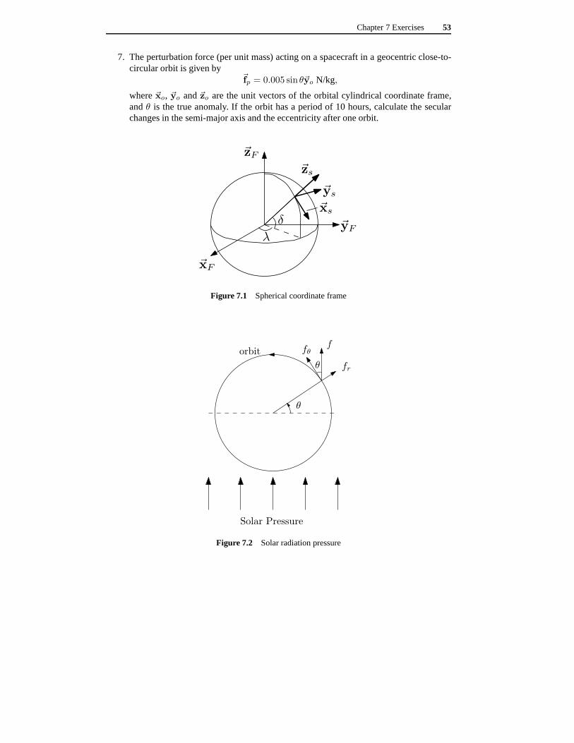
7. The perturbation force (per unit mass) acting on a spacecraft in a geocentric close-to-circular orbit is given by
~fp = 0.005 sin θ~yo N/kg,
where~xo, ~yo and~zo are the unit vectors of the orbital cylindrical coordinate frame,andθ is the true anomaly. If the orbit has a period of 10 hours, calculate the secularchanges in the semi-major axis and the eccentricity after one orbit.
~zF
~yFδ
λ
~xF
~xs
~zs
~ys
Figure 7.1 Spherical coordinate frame
θ
fr
ffθorbit
Solar Pressure
θ
Figure 7.2 Solar radiation pressure

54 Chapter 7 Exercises
orbit
Solar Pressure
θvθv
Earth
Figure 7.3 Shadowing by Earth

8Chapter 9 Exercises
For some of the following questions, you will need the Earth’s gravitational constant
µ = 3.986× 10⁵ km3/s2.
1. Prove the expressions in (9.29) in the book.
2. Prove the expression in (9.32) in the book.
3. Consider a geocentric leader-follower spacecraft formation, with the leader in acircular orbit of radiusrl = 7000 km. Determine the initial conditions for the followerspacecraft (in the Hill frame), if it is to be in a Projected Circular Orbit about theleader of radiusR = 100 m, with initial phase angleφ0 = 45o. Numerically simulatethe relative orbit using Hill’s equations to validate the initial conditions.
4. Repeat the development in Section 9.3.2 to obtain the initial conditions for a translatedProjected Elliptical Orbit, where everything is the same asin Section 9.3.2, except thatthe Projected Elliptical Orbit is to be centered at a pointx = xd, z = 0, wherexd isnon-zero.
5. Specialize the results from Question 4 to the case of a translated Projected CircularOrbit of radiusR.
6. Repeat Question 3 for a translated Projected Circular Orbit of the same dimension, butwith center atxd = 200 m.
7. Consider a geocentric leader-follower spacecraft formation, with the leader in a circularorbit of radiusrl = 7200 km. At the current time, the follower has position and velocityrelative to the leader given by (in Hill frame coordinates)
x = 234.2020 m, y = 70.7107 m, z = 66.9846 m,
x = −0.1281 m/s, y = 0.0731 m/s, z = 0.0177 m/s.
Determinex, z, P , φ,Q andα (using the notation from Sections 9.2.4 and 9.2.5 in thebook). Is the relative motion bounded?
8. In Sections 9.2.4 and 9.2.5 in the book, the following transformations were providedfrom x, y, z, x, y, z to x, z, P, φ,Q, α:
x = x− 2z
ωo,
Spacecraft Dynamics and Control - An Introduction,Anton H.J. de Ruiter, Christopher J. Damaren and James R. Forbes,c© 2013 John Wiley & Sons, Ltd. Published 2013 by John Wiley & Sons, Ltd.
Companion Website: http://www.wiley.com/go/deruiter/spacecraft

56 Chapter 9 Exercises
z = 4z +2x
ωo,
P =
(
(
3z +2x
ωo
)2
+
(
z
ω0
)2)
1
2
,
sinφ =−(
3z + 2xωo
)
P,
cosφ =z
ωoP,
Q =
(
y2 +
(
y
ω0
)2)
1
2
,
sinα =y
Q,
cosα =y
ωoQ.
Using only the expressions given above, prove the inverse transformations given below,from x, z, P, φ,Q, α to x, y, z, x, y, z:
x = x+ 2P cosφ,
z = z + P sinφ,
x = −ωo2
(3z + 4P sinφ) ,
z = ωoP cosφ,
y = Q sinα,
y = ωoQ cosα.
9. In Chapter 3 in the book, it was shown that the classical orbital elements provide muchgreater physical insight into an orbit than do the inertial position and velocity vectors.Likewise, for a leader-follower formation, the quantitiesx, z, P, φ,Q, α provide muchgreater physical insight into the relative motion of a leader-follower formation than dox, y, z, x, y, z. The physical meanings ofx, z, P, φ,Q, α, were investigated in Sections9.2.3 to 9.2.5 in the book.
However,x, z, P, φ,Q, α were defined on the basis of natural formation motion, thatis, without any disturbances or spacecraft control forces.It was shown that under theseconditions,z, P,Q are constant, andx = −3ω0z/2 and φ = α = ωo. However, inpractise, just as for a geocentric orbit, there will be disturbances or intentional controlforces which will causez, P,Q to vary with time, and the rates of˙x, φ, α to also vary.Therefore, similar to the Gauss variational equations for the orbital elements, it will beuseful to obtain dynamic equations forx, z, P, φ,Q, α, when the follower spacecraft isunder the influence of external forces.

Chapter 9 Exercises 57
As shown in Question 8, by simply taking as definitions the transformations fromx, y, z, x, y, z to x, z, P, φ,Q, α (without any consideration of physical meaning,or whether or not there are disturbance forces), the inversetransformation fromx, z, P, φ,Q, α to x, y, z, x, y, z is also well-defined, and takes the same formregardless of whether or not there are disturbance forces.
Now, considering the forced equations of relative motion (equations (9.11) and (9.12)in the book)
x = −2ωoz + fx,
z = 2ωox+ 3ω2oz + fz,
y = −ω2oy + fy,
show that the dynamics forx, z, P, φ,Q, α are given by
˙x = −3ωo2z − 2
ωofz,
˙z =2
ωofx,
P = −2 sinφ
ωofx +
cosφ
ωofz,
φ = ωo −2 cosφ
ωoPfx −
sinφ
ωoPfz,
Q =cosα
ωofy,
α = ωo −sinα
ωoQfy.


9Chapter 10 Exercises
1. Determine the extension of Equations (10.4) and (10.5) whenm3 is no longer confinedto the plane of the orbit ofm1 andm2.
2. Using numerical root-finding software, validate the locations ofL1, L2, andL3 for theEarth-Moon system.
3. Consider Equations (10.13) and (10.14) and adopt the nondimensionalizations
δx = δx/r12
δy = δy/r12
( ˙ ) =d( )
dτ, τ = ωt
(We have redefined the symbol( ˙ )). Show that the equations for the triangleequilibrium pointsL4 andL5 become
δ¨x − 2δ ˙y − 3
4δx− 3
√3
2
(
ρ− 1
2
)
δy = 0
δ¨y + 2δ ˙x− 3√3
2
(
ρ− 1
2
)
δx− 9
4δy = 0
for L4 and
δ¨x − 2δ ˙y − 3
4δx+
3√3
2
(
ρ− 1
2
)
δy = 0
δ¨y + 2δ ˙x+3√3
2
(
ρ− 1
2
)
δx− 9
4δy = 0
for L5, whereρ = m2/(m1 +m2). Determine the range of mass ratiosρ leading tostability of the triangle points. In particular, verify that they are stable for the Earth-Moon system whereρ = 0.01215.
Spacecraft Dynamics and Control - An Introduction,Anton H.J. de Ruiter, Christopher J. Damaren and James R. Forbes,c© 2013 John Wiley & Sons, Ltd. Published 2013 by John Wiley & Sons, Ltd.
Companion Website: http://www.wiley.com/go/deruiter/spacecraft


10Chapter 12 Exercises
1. A spacecraft with a principal axes body-fixed frameFb, has corresponding principalmoments of inertiaIx = 100 kg·m2, Iy = 120 kg·m2, Iz = 80 kg·m2. The spacecraftattitude relative to the Earth centered inertial frameFG is described by a yaw-pitch-roll(3-2-1) Euler sequence, represented by the rotation matrix
CbG(φ, θ, ψ) =
cθcψ cθsψ −sθsφsθcψ − cφsψ sφsθsψ + cφcψ sφcθcφsθcψ + sφsψ cφsθsψ − sφcψ cφcθ
wheresb = sin b andcb = cos b. Whereφ, θ andψ are the roll, pitch and yaw angles,respectively. Currently, the attitude is represented byφ = θ = ψ = π
4 rad, and thespacecraft orbital position (in ECI coordinates) is
~Ro = ~FTG
00Ro
km.
Determine the gravity-gradient torque acting on the spacecraft. Express the resultin spacecraft body coordinates. Note thatµ = 3.986× 10⁵ km3/s2 is the Earth’sgravitational constant.
2. The International Geomagnetic Reference Field (IGRF) isa global model of the Earth’smagnetic field. The IGRF model gives the Earth magnetic field vector at the spacecraftposition~r in spherical coordinates, where the spherical coordinate frameFs is definedas shown in Figure 10.1. That is, the IGRF model providesBr, Bθ andBλ such that
~B = ~FTs Bs = Bθ~xs +Bλ~ys +Br~zs.
The magnetic field componentsBr, Bθ andBλ are functions of the spacecraft orbitalradiusr, the spacecraft geocentric longitudeλ and the spacecraft geocentric co-latitudeθ = 90o − δ (δ is the geocentric latitude), as shown in Figure 10.2. For example, thefirst set of terms of the IGRF model are given by the dipole approximation
Br = 2(
Re
r
)3 [g01 cos θ +
(
g11 cosλ+ h11 sinλ)
sin θ]
,
Bθ =(
Re
r
)3 [g01 sin θ −
(
g11 cosλ+ h11 sinλ)
cos θ]
,
Bλ =(
Re
r
)3 [g11 sinλ− h11 cosλ
]
,
Spacecraft Dynamics and Control - An Introduction,Anton H.J. de Ruiter, Christopher J. Damaren and James R. Forbes,c© 2013 John Wiley & Sons, Ltd. Published 2013 by John Wiley & Sons, Ltd.
Companion Website: http://www.wiley.com/go/deruiter/spacecraft

62 Chapter 12 Exercises
where Re is the Earth’s equatorial radius, andg01 , g11 and h11 are given IGRFcoefficients.
Let the spacecraft have residual magnetic dipole moment~m = ~FTb mb, where the com-
ponentsmb in the spacecraft body frame are given. Also given are the spacecraftinertial attitudeCbG, and the spacecraft orbital position vector in ECI coordinates~r = ~FT
Gr.
Write down the equations required to compute the residual magnetic disturbancetorque in spacecraft body coordinates, using only the giveninformationmb, CbG andr (as well as the magnetic field parametersg01 , g11 andh11 and the Earth’s equatorialradius,Re, and rate of rotationωearth).
Note: As shown in Figure 10.2, the Earth Centered Earth Fixed(ECEF) frameFFis obtained from the Earth Centered Inertial (ECI) frameFG by a rotation about thez-axis through an angleαG = ωearth(t− t0), which is known as the right ascensionof the Greenwich meridian, andωearth is the rate of rotation of the earth. It is clear thatthe spacecraft geocentric longitude is given byλ = α− αG, whereα is the spacecraftright ascension.
3. Consider a flat surfaceS illuminated by the sun as shown in Figure 10.3. The surfacehas normal vector~n, and the unit vector pointing from the surface to the sun is~s.
(a) Show that the torque about the pointc due to the solar pressure on the side ofSwith outward normal~n is given by
~TS =
~ρA × ~FS , ~n ·~s ≥ 0,~0, ~n ·~s < 0.
where~ρA =
∫
S
~ρdSA
is the center of area ofS, A =∫
SdS is the area ofS,
~FS = −pA(~n ·~s)~s is the total solar pressure force onS andp is the solar pressuremagnitude.
(b) The surface of a spacecraft may be approximated by a number of flat surfacesS1, S2,....Sn. Each surface has areaAi, outward pointing normal vector given inbody coordinates as~ni = ~FT
b ni, and center of area located from the spacecraftcenter of mass also given on body coordinates as~ρA,i = ~FT
b ρA,i for i = 1, ..., n.
If the sun pointing vector is given in inertial coordinates as~s = ~FTI sI , obtain
the expression required to compute the total solar pressuretorque about thespacecraft center of mass in body coordinates.
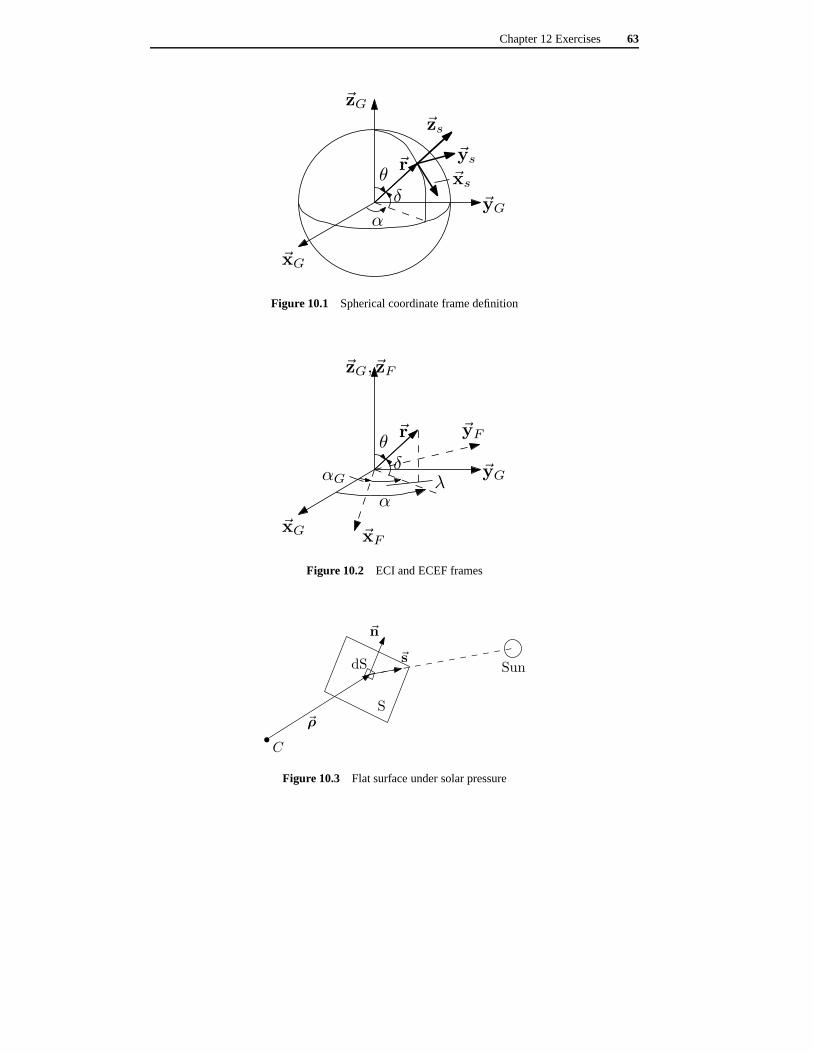
Chapter 12 Exercises 63
~zG
~yGδ
α
~xG
~xs
~zs
~ys
θ~r
Figure 10.1 Spherical coordinate frame definition
~zG,~zF
~yGδ
α
~xG
θ~r
~xF
~yF
λαG
Figure 10.2 ECI and ECEF frames
dS
S
~n
~s
~ρ
C
Sun
Figure 10.3 Flat surface under solar pressure


11Chapter 13 Exercises
1. A spacecraft is launched into a low Earth orbit. The spacecraft principal moments ofinertia areIx = 98 kg·m2, Iy = 102 kg·m2, Iz = 150 kg·m2. For stability, the launchvehicle deploys the spacecraft such that it is in a major axisspin when released, withωz = 0.5 rad/s. Because no deployment is perfect, the spacecraft also has some angularvelocity about the other two principal axes, given byωx = 0.1 rad/s,ωy = 0.02 rad/s.Making appropriate approximations:
(a) Describe the resulting spacecraft attitude motion if there are no disturbancetorques.
(b) Determine the nutation angle.
(c) Determine the precession rate.
2. A uniform thin disk is thrown into the air, and is observed to wobble such that its axisof symmetry traces out a cone with half angle 60o, once per second.
(a) Show that the transverse and axial moments of inertia of an uniforminfinitesimally thin disk satisfy
It =1
2Ia.
Assume that the disk has uniform mass per unit areaσ.
(b) Determine the relative spin-rate of the disk.
(c) Determine the disk angular velocity vector in inertial coordinates.
Spacecraft Dynamics and Control - An Introduction,Anton H.J. de Ruiter, Christopher J. Damaren and James R. Forbes,c© 2013 John Wiley & Sons, Ltd. Published 2013 by John Wiley & Sons, Ltd.
Companion Website: http://www.wiley.com/go/deruiter/spacecraft


12Chapter 14 Exercises
1. Consider a spacecraft with principal inertias satisfying Ix > Iz > Iy. Sometimes itmay be necessary to spin the spacecraft about the intermediate axis (in this case theprincipal z-axis). One method to accomplish this could be to apply control torquesTcx = −kωx, Tcy = −kωy andTcz = −ks (ωz − ν), whereν is the desired spin-rateabout the bodyz-axis. The equations of motion become
Ixωx + (Iz − Iy)ωyωz = Tcx,Iyωy + (Ix − Iz)ωxωz = Tcy,Izωz + (Iy − Ix)ωxωy = Tcz.
(a) Find the values ofk and ks that make a spin about the intermediate axisasymptotically stable.
(b) Is the feedbackTcz = −ks (ωz − ν) necessary to stabilize the intermediate axisspin?
2. Consider a rigid axisymmetric spinning body with principal moments of inertiaIx =Iy = It andIa = Iz.
(a) Show that the rotational kinetic energy is given by
T =h2
2
(
sin2 γ
It+
cos2 γ
Ia
)
,
whereh is the magnitude of the total angular momentum andγ is the anglebetween the axis of symmetry (~zb) and the angular momentum vector~h.Note: for a rigid body, the rotational kinetic energy is given by T = 1
2Ixω2x +
12Iyω
2y +
12Izω
2z .
(b) Under the Energy Sink Hypothesis, internal energy dissipation results in areduction in rotational kinetic energy, while the angular momentum is conserved.That is,T < 0 andh = constant. Show that under the energy-sink hypothesisfor an axisymmetric quasi-rigid body,
T =h2 sin 2γ
2IaIt(Ia − It) γ < 0,
for γ 6= 0, 90o.
Spacecraft Dynamics and Control - An Introduction,Anton H.J. de Ruiter, Christopher J. Damaren and James R. Forbes,c© 2013 John Wiley & Sons, Ltd. Published 2013 by John Wiley & Sons, Ltd.
Companion Website: http://www.wiley.com/go/deruiter/spacecraft

68 Chapter 14 Exercises
(c) Noting that we can always choose the~zb-axis such that0 ≤ γ ≤ 90o, explainhow the result obtained in part (b) is consistent with the major axis rule.

13Chapter 15 Exercises
1. Find all equilibrium solutions for a dual-spin satellitewith dynamics given by
Ixωx + (Iz − Iy)ωyωz + hsωy = 0,Iyωy + (Ix − Iz)ωxωz − hsωx = 0,Izωz + (Iy − Ix)ωxωy = 0.
2. Consider an axisymmetric dual-spin satellite, with principal inertiasIx = Iy = It andIz = Ia. The wheel spin axis coincides with the satellite axis of symmetry, namely theprincipalz-axis. The wheel has a positive constant spin angular momentum relative tothe spacecrafths > 0. The spacecraft is nominally non-spinning, that isωz(0) = 0.
(a) Obtain the solution for the resulting torque-free attitude motion.
(b) Provide a physical interpretation of the resulting torque-free attitude motion,analogous to that obtained in Section 13.2 in the book.
(c) Supposehs = 1 Nms,It = 10 kg·m2 andIa = 12 kg·m2, and the spacecraftz-axis is observed to trace out a cone in inertial space with half-angle 30o. Howlong does it take to trace out a single cone?
3. Consider a nominally non-spinning dual-spin spacecraftwith principal inertiasIx, IyandIz . The wheel axis coincides with the~zb axis of a body-fixed principal axes frame.The wheel relative angular momentum is given byhs > 0.
(a) Show that this situation corresponds to an equilibrium for torque-free motion.
(b) Show that small perturbations to the spacecraft angularvelocity lead to purelyoscillatory behavior inωx andωy with frequency
Ωp =hs
√
IxIy.
4. A spacecraft with principal axes body frameFb, has corresponding principal momentsof inertiaIx = 8 kg·m2, Iy = 12 kg·m2, Iz = 10 kg·m2.
It is desired to spin the spacecraft about the principal z-axis with angular velocityωz = 0.1 rad/s. Assuming that the spacecraft has a momentum wheel with spin-axis aligned with the principal z-axis, determine the required relative wheel angular
Spacecraft Dynamics and Control - An Introduction,Anton H.J. de Ruiter, Christopher J. Damaren and James R. Forbes,c© 2013 John Wiley & Sons, Ltd. Published 2013 by John Wiley & Sons, Ltd.
Companion Website: http://www.wiley.com/go/deruiter/spacecraft

70 Chapter 15 Exercises
momentumhs to make the desired attitude motion passively stable under torque-freeconditions.
5. Chapter 2, Question 3.
6. Chapter 2, Question 4.

14Chapter 16 Exercises
1. Chapter 2, Question 2
2. Consider an arbitrary spacecraft body frameFb (not necessarily a principal axesframe). That is, the spacecraft inertia matrix evaluated inFb has the form
I =
Ixx Ixy IxzIxy Iyy IyzIxz Iyz Izz
.
Let the spacecraft body-frameFb coincide with the orbiting reference frameFo for acircular orbit about earth. That is, the spacecraft has angular velocity
~ωbI = ~FTb ωbI , ωbI =
0−ωo0
,
whereωo =√
µ/r3 is the orbital angular velocity,µ is Earth’s gravitational constantandr is the spacecraft orbital radius.
(a) Show that the gravity-gradient torque vector in spacecraft body coordinates isgiven by
Tg = 3ω2o
−IyzIxz0
.
(b) Evaluateω×bIIωbI .
(c) Making use of parts (a) and (b) in the equations of motion,what are therequirements on the inertia matrixI for an earth-pointing equilibrium (Fb = Fo)in the presence of gravity-gradient torque? What does this say aboutFb?
3. Consider the spacecraft shown in Figure 14.1. The spacecraft hub is a solid cubic blockof mass 100 kg and side 1 m. To provide gravity-gradient stability, the spacecraft inertiais augmented by the addition of four lump masses of equal massm, located from thespacecraft center of mass by massless rods of lengthl.
(a) Determine the moment of inertia matrix for the spacecraft in terms ofm andl.
Spacecraft Dynamics and Control - An Introduction,Anton H.J. de Ruiter, Christopher J. Damaren and James R. Forbes,c© 2013 John Wiley & Sons, Ltd. Published 2013 by John Wiley & Sons, Ltd.
Companion Website: http://www.wiley.com/go/deruiter/spacecraft

72 Chapter 16 Exercises
(b) Based on the result of part (a), is the spacecraft gravity-gradient stabilized?
(c) In addition to the gravity-gradient torque, there is a constant solar pressure torqueabout the pitch axis given byTd,y = 10−5 Nm. Assuming that the spacecraft isin a circular orbit, andθ(0) = θ(0) = 0, find the solution for the pitch angleθ(t)in terms of the orbital rateωo, the massm and the rod lengthl.
(d) Assume now that the spacecraft is in a circular orbit witha period of 6 hours.How long must the rods be to ensure that the maximum excursionin pitch islimited to5o? Assume thatm = 2 kg.
m m
m m
l l
ll
60o
60o
60o
60o
~xb
~zb
appendage 1appendage 2
appendage 3 appendage 4
Figure 14.1 Satellite with inertia augmentation for Question 3

15Chapter 17 Exercises
1. Consider a spin-stabilized spacecraft nominally spinning about the principalz-axiswith spin-rateν. The desired angular velocities are thereforeωx = 0, ωy = 0 andωz = ν. It may be desirable to control the spin-rate. The equationsof motion are (asusual)
Ixωx + (Iz − Iy)ωyωz = Tcx + Tdx,Iyωy + (Ix − Iz)ωxωz = Tcy + Tdy,Izωz + (Iy − Ix)ωxωy = Tcz + Tdz.
whereTc. are control torques, andTd. are disturbance torques. The principal momentsof inertia areIx = 10 kg·m2, Iy = 12 kg·m2, Iz = 8 kg·m2.
(a) Assuming small angular velocitiesωx = ǫx, ωy = ǫy, obtain the linearizedequation for the spin-rateωz.
(b) Given that the output of interest isy = ωz, and the control input isu = Tcz, findthe plant transfer functionGp(s) such that
Y (s) = Gp(s)[
U(s) + Tdz(s)]
.
(c) The reference signal is the desired spin-rater = ν. Therefore, the spin-rate erroris e = ν − ω = r − y. Assuming proportional control
u(t) = Kpe(t),
Draw a block-diagram for the closed-loop system.(d) Find the closed-loop transfer function relationships from the reference signal
R(s) to the errorE(s) and from the disturbanceTdz(s) to the errorE(s). Whatrestriction must be placed on the proportional gainKp to ensure asymptoticstability?
(e) Find the responsee(t) to a step disturbanceTdz(t) = Tdz. What restriction mustbe placed on the proportional gainKp if the steady-state error to a disturbance ofmagnitudeTdz = 10−5Nm is to be kept below 1 deg/s?
(f) Find the responsee(t) to a step reference signalr(t) = ν. What restriction mustbe placed on the proportional gainKp if the spin-ratey(t) is to be within 2% ofthe desired spin-rateν within 10 seconds?
Spacecraft Dynamics and Control - An Introduction,Anton H.J. de Ruiter, Christopher J. Damaren and James R. Forbes,c© 2013 John Wiley & Sons, Ltd. Published 2013 by John Wiley & Sons, Ltd.
Companion Website: http://www.wiley.com/go/deruiter/spacecraft

74 Chapter 17 Exercises
2. Consider the spacecraft attitude control problem for a single axis. The attitudedynamics are given by
Iθ = u+ Td,
whereI is the related moment of inertia,θ is the related attitude angle,u is the controltorque applied about the axis by an actuator, andTd is a disturbance torque. Theactuator has dynamics
u = − 1
Ta(u− uc) ,
whereu is the control torque applied by the actuator,Ta is the actuator time constant,anduc is the control torque commanded by the control law.
(a) Find the actuator transfer function.
(b) The control law is chosen to be a modified PD control law
uc = Kpe(t)−Kdy(t),
where the plant output is the attitude angle (y(t) = θ(t)), the reference signal isthe desired attitude angle (r(t) = θd), ande(t) = r(t) − y(t) is the attitude error.
Draw a block diagram representation of the closed-loop system.
(c) Find the transfer function from reference signalR(s) to outputY (s), and thetransfer function from disturbanceTd(s) to outputY (s).
3. Consider the spacecraft attitude control problem for a single axis. Neglecting thedisturbance torque, the attitude dynamics are given by
Iθ = u,
whereu is the control torque. The moment of inertia isI = 1 kg·m2.
The following transient specifications are given for the closed-loop step response:
• Maximum overshoot requirement,Mp = 20%
• Settling time requirement,ts = 60 seconds
Design a modified PD control law such that the transient specifications are satisfied.
4. Consider the modified proportional-derivative attitudecontrol about a single spacecraftaxis as shown in Figure 15.1, whereI = 10 kg ·m2 is the corresponding moment ofinertia,y = θ is the corresponding attitude angle,r = θd is the desired attitude angle,Kp = 0.1 is the proportional gain andKd = 0.5 is the derivative gain. With regards toa unit step input:
(a) Determine the settling time.
(b) Determine the percent overshoot.
(c) Determine the rise time.
(d) Is it possible to reduce both the settling time and percent overshoot withoutchanging the proportional gain? Illustrate your reasoningwith a diagram.
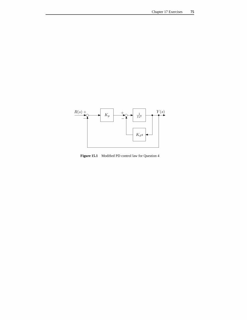
Chapter 17 Exercises 75
R(s) +
−
Kp
Y (s)+
−
Kds
1
Is2
Figure 15.1 Modified PD control law for Question 4


16Chapter 18 Exercises
1. A plant has transfer function
Gp(s) =Y (s)
U(s)=
1
s (s3 + s2 + 2s+ 1).
The plant is to be controlled using a controllerU(s) = Gc(s)E(s), as shown in Figure16.1.
(a) A proportional controlGc(s) = Kp is proposed. Determine the range ofproportional gain,Kp over which the closed-loop system is asymptotically stable.
(b) What is the system type with proportional control?(c) What are the steady-state errors of the closed-loop system to unit step and ramp
inputs whenKp =12? What are they whenKp = 2?
2. A plant has transfer function
Gp(s) =Y (s)
U(s)=
s+ 1
s2 (s2 + 2s+ 2).
The plant is to be controlled using a controllerU(s) = Gc(s)E(s), as shown in Figure16.1.
(a) Determine the closed-loop transfer functionY (s)R(s) , when the control is
proportional, that is whenGc(s) = Kp.(b) Using a Routh analysis, determine if it is possible to asymptotically stabilize the
system using proportional control only. If it can, determine the range ofKp thatmakes it asymptotically stable.
(c) Determine the closed-loop transfer functionY (s)R(s) when the control is
proportional-derivative, that is whenGc(s) = Kp + sKd.(d) Using a Routh analysis, determine conditions on the proportional gainKp to
asymptotically stabilize the system if the derivative gainisKd = 1.
3. Consider the small-angle roll-yaw equations for a nominally non-spinning dual-spinsatellite,
Ixφ− hsψ = Tx,
Izψ + hsφ = Tz.
Spacecraft Dynamics and Control - An Introduction,Anton H.J. de Ruiter, Christopher J. Damaren and James R. Forbes,c© 2013 John Wiley & Sons, Ltd. Published 2013 by John Wiley & Sons, Ltd.
Companion Website: http://www.wiley.com/go/deruiter/spacecraft

78 Chapter 18 Exercises
with proportional-derivative control for each axis
Tx = −Ix(
kpφ+ kdφ)
,
Tz = −Iz(
kpψ + kdψ)
.
(a) Show that the closed-loop roll and yaw poles satisfy the characteristic equation
s4 + 2kds3 +
(
2kp + k2d +h2sIxIz
)
s2 + 2kpkds+ k2p = 0.
(b) Using a Routh analysis, show that ifkp > 0 andkd > 0, the closed-loop roll andyaw equations are asymptotically stable.
R(s) E(s)+
−
U(s)Gc(s) Gp(s)
Y (s)
Figure 16.1 Feedback control system

17Chapter 19 Exercises
1. Consider the feedback control system in Figure 17.1. Assuming proportional controlGc(s) = K with K ≥ 0, sketch the root locus plots when the plant transfer functionsare:
(a)
Gp(s) =10
(s+ 1)(s+ 2)(s+ 3)
(b)
Gp(s) =1
(s+ 1)(s2 + 2s+ 2)
(c)
Gp(s) =s+ 2
(s+ 1)(s+ 3)(s+ 4)
(d)
Gp(s) =s+ 1
s2 + 2s+ 2
(e)
Gp(s) =s+ 3
(s+ 1)(s+ 2).
(f)
Gp(s) =1
(s+ 1)(s+ 2)(s2 + 2s+ 2)
(g)
Gp(s) =s2 + 4s+ 5
(s+ 1)(s+ 2)(s2 + 2s+ 2)
Spacecraft Dynamics and Control - An Introduction,Anton H.J. de Ruiter, Christopher J. Damaren and James R. Forbes,c© 2013 John Wiley & Sons, Ltd. Published 2013 by John Wiley & Sons, Ltd.
Companion Website: http://www.wiley.com/go/deruiter/spacecraft

80 Chapter 19 Exercises
Note: If there are asymptotes, compute the angles and center. Do not computebreakaway and break-in points or imaginary axis crossings.
2. Consider the small-angle roll-yaw equations for a nominally non-spinning dual-spinsatellite,
Ixφ− hsψ = Tx,
Izψ + hsφ = Tz.
with proportional-derivative control for each axis
Tx = −Ix(
kpφ+ kdφ)
,
Tz = −Iz(
kpψ + kdψ)
.
As found in Question 3, Chapter 18, the closed-loop roll and yaw poles satisfy thecharacteristic equation
s4 + 2kds3 +
(
2kp + k2d +h2sIxIz
)
s2 + 2kpkds+ k2p = 0.
(a) Show that the characteristic equation can be rewritten equivalently as
1 +h2sIxIz
s2
(s2 + kds+ kp)2 = 0.
(b) Assume that the gainskp andkd are chosen according tokd = 2ζωn andkp =ω2n, where0 < ζ < 1 is the desired damping ratio andωn is the desired undamped
natural frequency. Sketch a root-locus plot for the closed-loop poles as the wheel
angular momentum changes, that is, forh2
s
IxIz≥ 0. Compute the asymptote angles
and center, but do not compute any other details.
R(s) E(s)+
−
U(s)Gc(s) Gp(s)
Y (s)
Figure 17.1 Feedback control system

18Chapter 20 Exercises
Consider the feedback control system in Figure 18.1.
1. The plant has transfer function
Gp(s) =a
(s+ 1)(s+ 2)(s+ 3),
wherea > 0. Suggest a controllerGc(s) if the closed-loop system is to exhibit nooscillatory behavior (no complex closed-loop poles) regardless of the value ofa.
2. Consider again the plant with transfer function
Gp(s) =a
(s+ 1)(s+ 2)(s+ 3),
wherea > 0. What are the minimum number of zeros that must be contained in thecontrollerGc(s) such that the closed-loop system will never go unstable, regardless ofthe value ofa? Where must it be placed?
3. The plant has transfer function
Gp(s) =1
s+ 1.
The control lawGc(s) is to be designed such that the closed-loop system has dominantpoles ats = −3± j3, and a zero steady-state error to a step inputr(t) = 1.
(a) Can the control objective be met with pure integral control, Gc(s) = Ks
? Hint:do the desired dominant poles lie on the root locus?
(b) Design a combined lead-integral control
Gc(s) = K
(
s+ 1T
)
s(
s+ 1αT
) ,
with T > 0 and0 < α < 1. such that the closed-loop requirements are met. Youmay takeT = 1
3 . Hint: you may augment the plant with the integrator.
Spacecraft Dynamics and Control - An Introduction,Anton H.J. de Ruiter, Christopher J. Damaren and James R. Forbes,c© 2013 John Wiley & Sons, Ltd. Published 2013 by John Wiley & Sons, Ltd.
Companion Website: http://www.wiley.com/go/deruiter/spacecraft

82 Chapter 20 Exercises
R(s) E(s)+
−
U(s)Gc(s) Gp(s)
Y (s)
Figure 18.1 Feedback control system

19Bias Momentum Control DesignExercises - Chapters 17 to 20
The following exercises will involve the design of an attitude control system for a biasmomentum satellite, and ties together the subjects of Chapters 17 to 20.
BackgroundA bias momentum satellite is an earth-pointing dual-spin satellite, with attitude controlledrelative to an orbiting reference frameFo as shown in Figure 19.1. The momentum wheelspin axis is aligned with the orbit normal (an inertially fixed direction for a two-body orbit),making it a pitch wheel. We describe the spacecraft attituderelative to the orbiting frame by ayaw-pitch-roll (3-2-1) Euler sequence, whereφ, θ andψ denote the roll, pitch and yaw anglesrespectively. For small rotations,φ constitutes a rotation about~xo, θ is a rotation about~yoandψ is a rotation about~zo (as shown in Figure 19.1).
For many bias momentum satellites, the only attitude sensoris an Earth sensor. An Earthsensor gives the direction of the center of earth from the spacecraft (−~r) in body coordinates.The roll and pitch anglesφ andθ can be determined from this measurement. However, ascan be seen from Figure 19.1, if the spacecraft undergoes a pure yaw rotation, the rotationis about−~r, so it does not change in body coordinates. Therefore, the yaw angle cannot bemeasured by an earth sensor.
Bias momentum stabilization for an earth pointing satellite has the following benefits:
• Coupling between the roll and yaw axes due to the bias momentum. This means thatthe yaw angle can be stabilized without using a yaw sensor.
• Gyroscopic stability of the roll and yaw angles due to the bias momentum.
• The pitch wheel can be used to control the pitch angle (by changing it’s speed)
• The pitch wheel can be used to control roll and yaw angles (by making small changesto the spin axis (aka control moment gyro))
The equations of motion are given by
Iω + hsa+ ω× [Iω + hsa] = Tc +Td +Tg,
whereTc is the control torque,Td is the external disturbance torque,Tg is the gravity-gradient torque, and all other symbols have the same meaningas in the book. We take the
Spacecraft Dynamics and Control - An Introduction,Anton H.J. de Ruiter, Christopher J. Damaren and James R. Forbes,c© 2013 John Wiley & Sons, Ltd. Published 2013 by John Wiley & Sons, Ltd.
Companion Website: http://www.wiley.com/go/deruiter/spacecraft

84 Bias Momentum Control Design Exercises - Chapters 17 to 20
wheel spin-axis to be
a =
0−10
.
Assuming that the body frame is a principal axes frame, the spacecraft is in a circular orbit,and that the angles and rates are small, the equations of motion relative to the orbiting framebecome
Ixφ− [(Ix + Iz − Iy)ωo − hs] ψ +[
4(Iy − Iz)ω2o + ωohs
]
φ = Tcx + Tdx,
Iy θ + 3(Ix − Iz)ω2oθ = Tcy + Tdy,
Izψ + [(Ix + Iz − Iy)ωo − hs] φ+[
(Iy − Ix)ω2o + ωohs
]
ψ = Tcz + Tdz,
whereTcy = −hs if the momentum wheel is used to control the pitch, andωo =√
µ/r3 isthe orbital angular rate. These equations may be compared toequations (16.14) to (16.16) inthe book, for a gravity-gradient stabilized spacecraft.
Finally, we make the approximation that|Ixωo|, |Iyωo|, |Izωo| << |hs|, greatlysimplifying the equations of motion to
Ixφ+ hsψ + ωohsφ = Tcx + Tdx,
Iy θ + kgθ = Tcy + Tdy,
Izψ − hsφ+ ωohsψ = Tcz + Tdz,
wherekg = 3(Ix − Iz)ω2o . It can be seen that the pitch equation is decoupled from the roll
and yaw equations.
Spacecraft and Orbital ParametersThe spacecraft principal inertias areIx = 0.4 kg·m2, Iy = 0.5 kg·m2, Iz = 0.6 kg·m2. Thespacecraft is in a circular orbit with altitude600 km, such that the orbital angular rate isωo = 0.001083 rad/s. The expected maximum disturbance torques areTdx,max = Tdy,max =Tdz,max = 5× 10⁻⁶ Nm.
Control System Requirements
• The maximum allowable steady-state errors in response to constant disturbances areφss ≤ 0.1 deg,θss ≤ 0.1 deg andψss ≤ 4 deg.
• The closed-loop poles for the roll/yaw loop are to have damping ratiosζ = 0.7.
The spacecraft is expected to be capable of making pitch maneuvers, with transientspecification for a pitch step response:
• Settling-time,ts ≤ 200 seconds.
• Percent overshoot,Mp ≤ 30 %.
You will need the Earth’s gravitational constant
µ = 3.986× 10⁵ km3/s2,
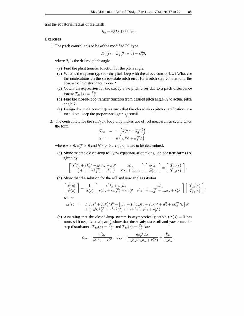
Bias Momentum Control Design Exercises - Chapters 17 to 2085
and the equatorial radius of the Earth
Re = 6378.1363 km.
Exercises
1. The pitch controller is to be of the modified PD type
Tcy(t) = kpp(θd − θ)− kpd θ,
whereθd is the desired pitch angle.
(a) Find the plant transfer function for the pitch angle.(b) What is the system type for the pitch loop with the above control law? What are
the implications on the steady-state pitch error for a pitchstep command in theabsence of a disturbance torque?
(c) Obtain an expression for the steady-state pitch error due to a pitch disturbancetorqueTdy(s) =
Tdy
s.
(d) Find the closed-loop transfer function from desired pitch angleθd to actual pitchangleθ.
(e) Design the pitch control gains such that the closed-looppitch specifications aremet. Note: keep the proportional gainkpp small.
2. The control law for the roll/yaw loop only makes use of rollmeasurements, and takesthe form
Tcx = −(
kryp φ+ kryd φ)
,
Tcz = a(
kryp φ+ kryd φ)
,
wherea > 0, kryp > 0 andkryd > 0 are parameters to be determined.
(a) Show that the closed-loop roll/yaw equations after taking Laplace transforms aregiven by[
s2Ix + skryd + ωohs + kryp shs−(
s(hs + akryd ) + akryp)
s2Iz + ωohs
] [
φ(s)
ψ(s)
]
=
[
Tdx(s)
Tdz(s)
]
.
(b) Show that the solution for the roll and yaw angles satisfies[
φ(s)
ψ(s)
]
=1
∆(s)
[
s2Iz + ωohs −shss(hs + akryd ) + akryp s2Ix + skryd + ωohs + kryp
] [
Tdx(s)
Tdz(s)
]
,
where
∆(s) = IxIzs4 + Izk
ryd s
3 +[
(Ix + Iz)ωohs + Izkryp + h2s + akryd hs
]
s2
+[
ωohskryd + ahsk
ryp
]
s+ ωohs(ωohs + kryp ).
(c) Assuming that the closed-loop system is asymptoticallystable (∆(s) = 0 hasroots with negative real parts), show that the steady-stateroll and yaw errors forstep disturbancesTdx(s) = Tdx
sandTdz(s) = Tdz
sare
φss =Tdx
ωohs + kryp, ψss =
akryp Tdx
ωohs(ωohs + kryp )+
Tdzωohs
.

86 Bias Momentum Control Design Exercises - Chapters 17 to 20
(d) Typically, the control system shall be designed such that a < 1 and kryp >>ωohs. Therefore, the yaw error may be upper-bounded by
|ψss| ≤|Tdx|+ |Tdz|
ωo|hs|.
Using this approximation, and the expression forφss from part (c), determine therequired bias momentumhs and the proportional gainkryp such that the roll andyaw steady-state specifications are satisfied. Note: takehs, k
ryp > 0.
(e) Having selectedhs andkryp , all that remains is to selectkryd anda such that theclosed-loop poles have the required damping ratio. This is done as follows. Frompart (b), the closed-loop poles satisfy the characteristicequation
∆(s) = 0.
We would like the closed-loop poles to bes = −ζωn1 ± jωn1√
1− ζ2,−ζωn2 ±jωn2
√
1− ζ2, whereζ is the required damping ratio of the poles, andωn1 andωn2 are the undamped natural frequencies of the poles. Therefore, the character-istic equation should have the form
(s2 + 2ζωn1s+ ω2n1)(s
2 + 2ζωn2s+ ω2n2) = 0.
To find the requiredkryd anda, we equate
∆(s) = IxIz(s2 + 2ζωn1s+ ω2
n1)(s2 + 2ζωn2s+ ω2
n2).
Equating the coefficients of powers ofs, leads to four equations in fourunknowns, namelykryd , a, ωn1 andωn2 (the damping rationζ is given). We areonly interested in the first two.
i. Show that the solutions forkryd anda are
kryd =
√
E (B − (4ζ2 − 2)F )
EA2 − C(AF −D),
a =(AF −D)
Ekryd ,
where
A =1
2ζIx, B =
(Ix + Iz)hsωoIxIz
+krypIx
+h2sIxIz
,
C =hsIxIz
, D =ωohs2ζIxIz
, E =hsk
ryp
2ζIxIz,
F =
√
ωohs(ωohs + kryp )
IxIz.
ii. Find kryd anda.

Bias Momentum Control Design Exercises - Chapters 17 to 2087
3. The pitch control command obtained in question 1 is to be applied by an actuator withdynamics
Tcy(s) =1
Ts+ 1Uc(s),
whereT > 0 is the actuator time constant,Uc(s) is the control torque commandedby the control law given in Question 1, andTcy(s) is the pitch torque applied to thespacecraft by the actuator.
(a) Show that the characteristic equation for the closed-loop system is
IyTs3 + Iys
2 + (kgT + kpd)s+ kg + kpp = 0.
(b) Determine the condition that the actuator time-constant T must satisfy for theclosed-loop system to be asymptotically stable.
(c) Sketch a root locus for the closed-loop poles for1T≥ 0. It does not need to
be to scale. Do not determine details like breakaway points and imaginary axiscrossings. Note: Be mindful of the sign ofkg. What can you conclude from theroot locus?
4. The pitch actuator is much slower than you had originally specified as the controlsystem designer, with a time constantT = 5 seconds. Is it possible to redesign thePD controller obtained in Question 1 so that the closed-loopsystem (when actuatordynamics are included) has the dominant poles you obtained in Question 1? If it ispossible, redesign the PD controller.
To simplify the problem, you may setkg = 0. To save some effort in finding the open-loop transfer function, note that the characteristic equation in part (a) of Question 3may be rewritten as (withkg = 0)
1 +kpdIyT
(s+kppkp
d
)
s2(s+ 1T)= 0.
From this, we can identify
Go(s) =kpdIyT
(s+kppkp
d
)
s2(s+ 1T),
as the open-loop transfer function,kp
d
IyTas the open-loop gain, ands = −kpp
kp
d
as the PDzero.
Hint for solving the problem: Check the maximum possible angle 6
(
s+kppkp
d
)
that thePD zero can provide, and compare it to what is required.

88 Bias Momentum Control Design Exercises - Chapters 17 to 20
~xo
~yo~zo
~h
~r
Earthorbit
φ
θψ
Figure 19.1 Orbiting Reference Frame

20Chapter 21 Exercises
1. Sketch the frequency responses (Bode plots) for the systems with transfer functions:
(a)
G(s) =10
(s+ 0.1)(s+ 1)(s+ 10)
(b)
G(s) =s+ 1
(s+ 0.1)(s+ 10)
(c)
G(s) =(s+ 1)(s+ 10)
(s+ 0.1)(s+ 100).
2. If a filterH(s) is to be designed such that low frequency inputs are passed, but highfrequency inputs are blocked, what is the requirement on thenumber of zeros and polesof H(s)?
Spacecraft Dynamics and Control - An Introduction,Anton H.J. de Ruiter, Christopher J. Damaren and James R. Forbes,c© 2013 John Wiley & Sons, Ltd. Published 2013 by John Wiley & Sons, Ltd.
Companion Website: http://www.wiley.com/go/deruiter/spacecraft

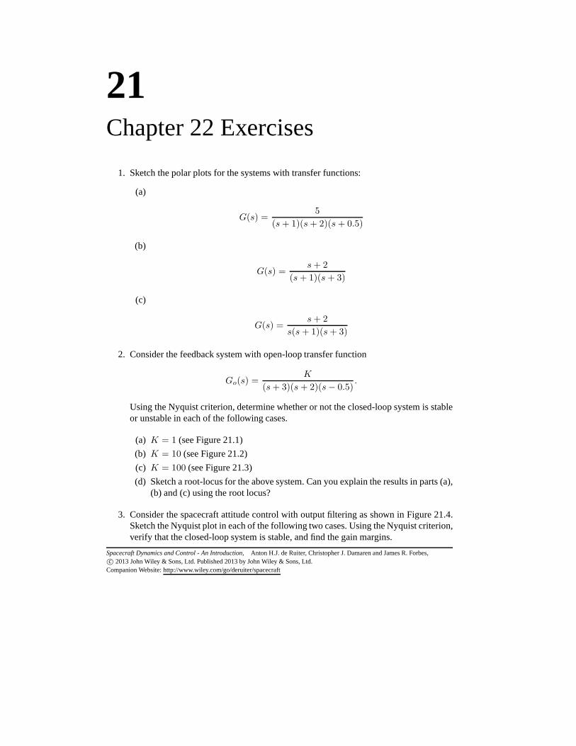
21Chapter 22 Exercises
1. Sketch the polar plots for the systems with transfer functions:
(a)
G(s) =5
(s+ 1)(s+ 2)(s+ 0.5)
(b)
G(s) =s+ 2
(s+ 1)(s+ 3)
(c)
G(s) =s+ 2
s(s+ 1)(s+ 3)
2. Consider the feedback system with open-loop transfer function
Go(s) =K
(s+ 3)(s+ 2)(s− 0.5).
Using the Nyquist criterion, determine whether or not the closed-loop system is stableor unstable in each of the following cases.
(a) K = 1 (see Figure 21.1)
(b) K = 10 (see Figure 21.2)
(c) K = 100 (see Figure 21.3)
(d) Sketch a root-locus for the above system. Can you explainthe results in parts (a),(b) and (c) using the root locus?
3. Consider the spacecraft attitude control with output filtering as shown in Figure 21.4.Sketch the Nyquist plot in each of the following two cases. Using the Nyquist criterion,verify that the closed-loop system is stable, and find the gain margins.
Spacecraft Dynamics and Control - An Introduction,Anton H.J. de Ruiter, Christopher J. Damaren and James R. Forbes,c© 2013 John Wiley & Sons, Ltd. Published 2013 by John Wiley & Sons, Ltd.
Companion Website: http://www.wiley.com/go/deruiter/spacecraft

92 Chapter 22 Exercises
(a) PD controlGc(s) = Kp +Kds.
Low pass filter
H(s) =1
Ts+ 1
System parameters:
I = 1, T = 1, Kp = 0.01, Kd = 0.1.
(b) PID control
Gc(s) = Kp +Kds+Ki
s.
Double low pass filter
H(s) =1
(Ts+ 1)2
System parameters:
I = 1, T = 1, Kp = 0.01, Kd = 0.1, Ki = 10−4.
4. Sketch the Bode plot corresponding to part (a) of Question3. Estimate the phasemargins and the allowable time-delay in the feedback loop.
5. Figure 21.5 shows the Bode plot corresponding to part (b) of Question 3. Estimate allstability margins.
−1 −0.8 −0.6 −0.4 −0.2 0−0.1
−0.08
−0.06
−0.04
−0.02
0
0.02
0.04
0.06
0.08
0.1
Nyquist Diagram
Real Axis
Imag
inar
y A
xis
Figure 21.1 Nyquist plot for Question 2(a),K = 1
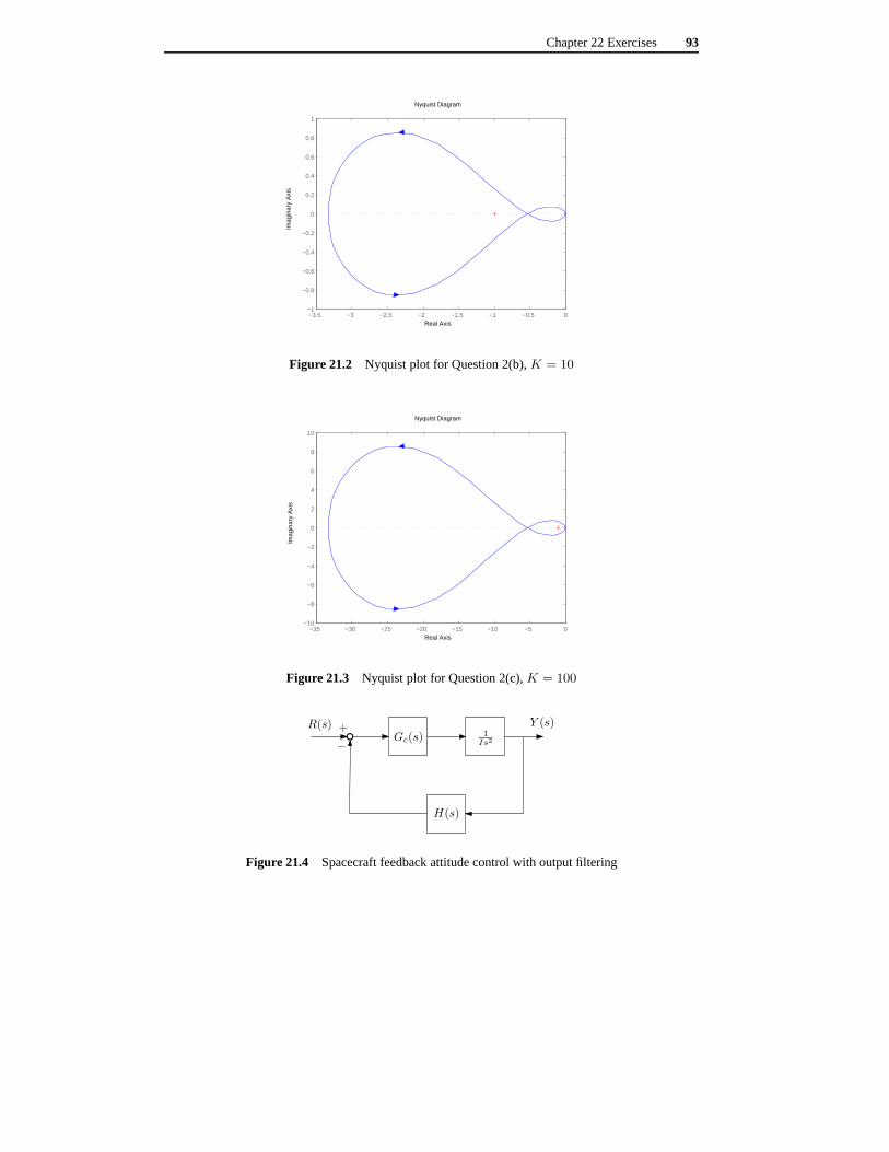
Chapter 22 Exercises 93
−3.5 −3 −2.5 −2 −1.5 −1 −0.5 0−1
−0.8
−0.6
−0.4
−0.2
0
0.2
0.4
0.6
0.8
1
Nyquist Diagram
Real Axis
Imag
inar
y A
xis
Figure 21.2 Nyquist plot for Question 2(b),K = 10
−35 −30 −25 −20 −15 −10 −5 0−10
−8
−6
−4
−2
0
2
4
6
8
10
Nyquist Diagram
Real Axis
Imag
inar
y A
xis
Figure 21.3 Nyquist plot for Question 2(c),K = 100
1
Is2Gc(s)
H(s)
Y (s)R(s) +
−
Figure 21.4 Spacecraft feedback attitude control with output filtering
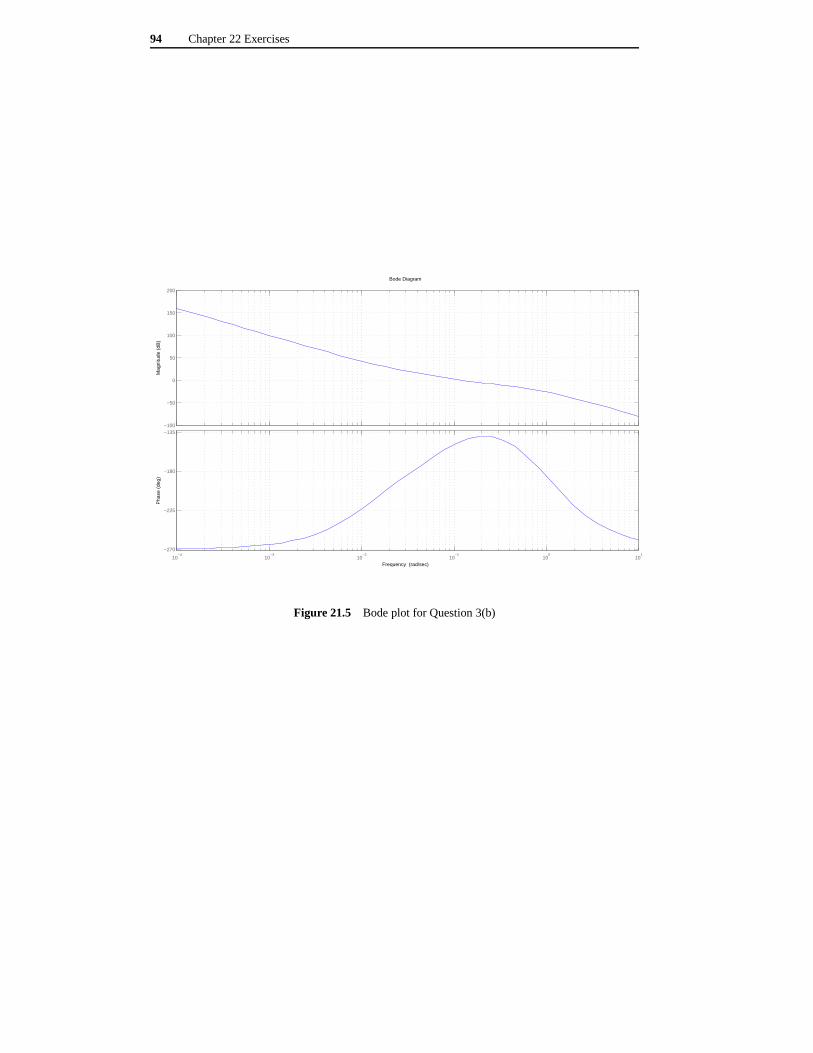
94 Chapter 22 Exercises
Bode Diagram
Frequency (rad/sec)10
−410
−310
−210
−110
010
1−270
−225
−180
−135
Pha
se (
deg)
−100
−50
0
50
100
150
200
Mag
nitu
de (
dB)
Figure 21.5 Bode plot for Question 3(b)
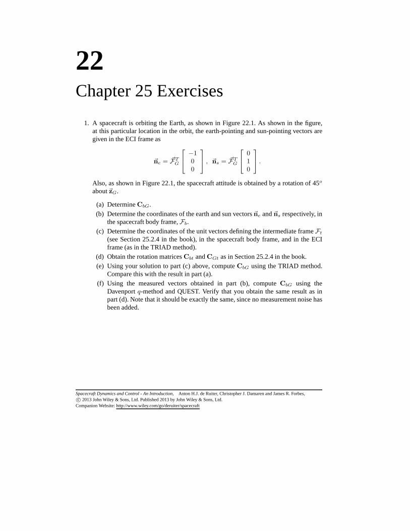
22Chapter 25 Exercises
1. A spacecraft is orbiting the Earth, as shown in Figure 22.1. As shown in the figure,at this particular location in the orbit, the earth-pointing and sun-pointing vectors aregiven in the ECI frame as
~ne = ~FTG
−100
, ~ns = ~FTG
010
.
Also, as shown in Figure 22.1, the spacecraft attitude is obtained by a rotation of 45o
about~zG.
(a) DetermineCbG.
(b) Determine the coordinates of the earth and sun vectors~ne and~ns respectively, inthe spacecraft body frame,Fb.
(c) Determine the coordinates of the unit vectors defining the intermediate frameFt(see Section 25.2.4 in the book), in the spacecraft body frame, and in the ECIframe (as in the TRIAD method).
(d) Obtain the rotation matricesCbt andCGt as in Section 25.2.4 in the book.
(e) Using your solution to part (c) above, computeCbG using the TRIAD method.Compare this with the result in part (a).
(f) Using the measured vectors obtained in part (b), computeCbG using theDavenportq-method and QUEST. Verify that you obtain the same result as inpart (d). Note that it should be exactly the same, since no measurement noise hasbeen added.
Spacecraft Dynamics and Control - An Introduction,Anton H.J. de Ruiter, Christopher J. Damaren and James R. Forbes,c© 2013 John Wiley & Sons, Ltd. Published 2013 by John Wiley & Sons, Ltd.
Companion Website: http://www.wiley.com/go/deruiter/spacecraft

96 Chapter 25 Exercises
Sun
Earth
Spacecraft
~yG
~xG ~ne
~yb~ns
~xb
45o
Figure 22.1 Attitude determination question