sparse reconstruction using distribution agnostic bayesian matching pursuit

5298 IEEE TRANSACTIONS ON SIGNAL PROCESSING, VOL. 61, NO. 21, NOVEMBER 1, 2013

Sparse Reconstruction Using DistributionAgnostic Bayesian Matching Pursuit

Mudassir Masood, Student Member, IEEE, and Tareq Y. Al-Naffouri, Member, IEEE

Abstract—A fast matching pursuit method using a Bayesian ap-proach is introduced for sparse signal recovery. This method per-forms Bayesian estimates of sparse signals even when the signalprior is non-Gaussian or unknown. It is agnostic on signal statisticsand utilizes a priori statistics of additive noise and the sparsity rateof the signal, which are shown to be easily estimated from data ifnot available. Themethod utilizes a greedy approach and order-re-cursive updates of its metrics to find themost dominant sparse sup-ports to determine the approximate minimum mean-square error(MMSE) estimate of the sparse signal. Simulation results demon-strate the power and robustness of our proposed estimator.

Index Terms—Basis selection, Bayesian, compressed sensing,greedy algorithm, linear regression, matching pursuit, minimummean-square error (MMSE) estimate, sparse reconstruction.

I. INTRODUCTION

S PARSITY is a feature that is abundant in both naturaland man-made signals. Some examples of sparse signals

include those from speech, images, videos, sensor arrays (e.g.,temperature and light sensors), seismic activity, galactic ac-tivities, biometric activity, radiology, and frequency hopping.Given the vast existence of signals, their sparsity is an attrac-tive property because the exploitation of this sparsity may beuseful in the development of simple signal processing systems.Some examples of systems in which a priori knowledge ofsignal sparsity is utilized include motion estimation [1], mag-netic resonance imaging (MRI) [2], impulse noise estimationand cancellation in DSL [3], network tomography [4], andpeak-to-average-power ratio reduction in OFDM [5], [25]. All

Manuscript received June 11, 2012; revised November 23, 2012, June23, 2013, and July 30, 2013; accepted July 31, 2013. Date of publicationAugust 15, 2013; date of current version September 23, 2013. The associateeditor coordinating the review of this manuscript and approving it for publi-cation was Dr. Piotr Indyk. This work was funded in part by a CRG2 grantCRG\_R2\_13\_ALOU\_KAUST\_2 from the Office of Competitive Research(OCRF) at King Abdullah University of Science and Technology (KAUST).The work of T.Y. Al-Naffouri was also supported by King Abdulaziz City forScience and Technology (KACST) through the Science & Technology Unitat King Fahd University of Petroleum & Minerals (KFUPM) through ProjectNo. 09-ELE763-04 as part of the National Science, Technology and InnovationPlan.M. Masood is with the Department of Electrical Engineering, King Abdullah

University of Science & Technology, Thuwal 23955-6900, Saudi Arabia(e-mail: [email protected]).T. Y. Al-Naffouri is with the Department of Electrical Engineering, King

Abdullah University of Science & Technology, Thuwal 23955-6900, SaudiArabia, and also with the Department of Electrical Engineering, King FahdUniversity of Petroleum and Minerals, Dhahran 31261, Saudi Arabia (e-mail:[email protected]).Color versions of one or more of the figures in this paper are available online

at http://ieeexplore.ieee.org.Digital Object Identifier 10.1109/TSP.2013.2278814

of these systems are based on sparsity-aware estimators such asLasso [6], basis pursuit [7], structure-based estimator [8], [26],fast Bayesian matching pursuit [9], and estimators related tothe relatively new area of compressed sensing [10]–[12].Compressed sensing (CS), otherwise known as compressive

sampling, has found many applications in the fields of commu-nications, image processing, medical imaging, and networking.CS algorithms have been shown to recover sparse signals fromunderdetermined systems of equations that take the form

(1)

where , and are the unknown sparse signal andthe observed signal, respectively. Furthermore, isthe measurement matrix and is the additive Gaussiannoise vector. Here, the number of unknown elements, , ismuch larger than the number of observations, . CS uses linearprojections of sparse signals that preserve structure of signals;furthermore, these projections are used to reconstruct the sparsesignal using -optimization with high probability.

(2)

where . -optimization is a convex op-timization problem that conveniently reduces to a linear pro-gram known as basis pursuit, which has the high computationalcomplexity of . Other more efficient algorithms such asorthogonal matching pursuit (OMP) [13] and the algorithm pro-posed by Haupt et al. [14] have been proposed. These algo-rithms fall into the category of greedy algorithms that are rel-atively faster than basis pursuit. However, it should be notedthat the only a priori information utilized by these systems isthe sparsity information.1

Another category of methods based on the Bayesian approachconsiders complete a priori statistical information of sparsesignals. The fast Bayesian matching pursuit (FBMP) [9], [15]adopts such an approach and assumes a Bernoulli-Gaussianprior on the unknown vector . This method performs sparsesignal estimation via model selection and model averaging. Thesparse vector is described as a mixture of several components,the selection of which is based on successive model expansion.FBMP obtains an approximate MMSE estimate of the unknownsignal with high accuracy and low complexity. It was shownto outperform several sparse recovery algorithms, includingOMP [13], StOMP [16], GPSR-Basic [17], Sparse Bayes [18],BCS [19] and a variational-Bayes implementation of BCS

1The advantage of these approaches is that they are distribution agnostic andhence demonstrate robust performance.

1053-587X © 2013 IEEE

MASOOD AND AL-NAFFOURI: SPARSE RECONSTRUCTION USING DISTRIBUTION AGNOSTIC BAYESIAN MATCHING PURSUIT 5299

[20]. However, there are several drawbacks associated withthis method. The assumption that the support distribution2 isGaussian is not realistic, because, in most real-world scenarios,it is not Gaussian, or it is unknown. In addition, its performanceis dependent on the knowledge of parameters of the Gaussianand Bernoulli priors, which are usually difficult to compute.Although a parameter estimation process is proposed, it isdependent on knowledge of the initial estimates of these signalparameters. The estimation process, in turn, has a negativeimpact on the complexity of the method.Another popular Bayesian method proposed by Larsson

and Selén [21] computes the MMSE estimate of the unknownvector, . Its approach is similar to that of FBMP in the sensethat the sparse vector is described as a mixture of several com-ponents that are selected based on successive model reduction.It also requires knowledge of the noise and signal statistics.However, it was found that the MMSE estimate is insensitiveto the a priori parameters and therefore an empirical-Bayesianvariant that does not require any a priori knowledge of the datawas devised.Babacan et al. [22] have also proposed a greedy algorithm

based on a Bayesian framework. They utilize a hierarchical formof the Laplace prior to model the sparsity of unknown signal.Their fast approach is fully automatic and does not require userintervention. They have also shown that their technique outper-forms several sparse recovery algorithms. The list includes all ofthe algorithmswhich FBMP used to compare their performance.The Bayesian approaches mentioned above in [9], [15] and

[21] assume Gaussian prior on the non-zero elements of the un-known sparse vector3 , while the Bayesian approach of [22]assumes a Laplace prior. It is reasonable to assume that any ad-ditive noise, generated at the sensing end, is Gaussian. How-ever, assuming the signal statistics to be Bernoulli-Gaussian orLaplacian does not always reflect reality. Moreover, regardlessof whether the actual prior is Gaussian or not, the parameters(mean and variance) of the Gaussian prior to be used need tobe estimated, which is challenging especially when the signalstatistics are not i.i.d. In that respect, one can appreciate convexrelaxation approaches that are agnostic to signal statistics.In this paper, we pursue a Bayesian approach for sparse

signal reconstruction that combines the advantages of the twoapproaches summarized above. On the one hand, the approachis Bayesian, acknowledging the noise statistics and the signalsparsity rate, while on the other hand, the approach is agnosticto the support distribution. While the approach depends on thesparsity rate and the noise variance, it does not require estimatesof the parameters but is able to estimate these parameters in arobust manner. Specifically, the advantages of our approach areas follows1) The approach provides a Bayesian estimate of the sparsesignal even when the signal support prior is non-Gaussianor unknown.

2) The approach is agnostic to the support distribution and sothe parameters of this distribution whether Gaussian or not

2In the paper we use the term support distribution to refer to the distributionof the active elements of .3While the Bayesian approaches of [9], [15], and [21] assume a Gaussian

prior, these approaches continued to work when this assumption is violated.

need not be estimated. This is particularly useful when thesignal support priors are not i.i.d. Therefore, it is agnosticto variations in distributions.

3) The approach utilizes the prior Gaussian statistics of theadditive noise and the sparsity rate of the signal. The ap-proach is able to estimate the noise variance and sparsityrate in a robust manner from the data.

4) The approach enjoys low complexity thanks to its greedyapproach and the order-recursive update of its metrics.

The fact that our approach is agnostic to support distributionmotivates us to call it Support Agnostic Bayesian MatchingPursuit (SABMP). The remainder of this paper is organized asfollows. In Section II, we formulate the problem and presentthe MMSE setup in the non-Gaussian/unknown statistics case.In Section III, we describe our greedy algorithm that is able toobtain the approximate MMSE estimate of the sparse vectorfollowed by a description of our hyperparameter estimationprocess. Section IV demonstrates how the greedy algorithmcan be made faster by calculating various metrics in a recursivemanner. This is followed by Section V in which we present oursimulation results and in Section VI, we conclude the paper.

A. Notation

We denote scalars with small-case letters (e.g., ), vectorswith small-case, bold-face letters (e.g., ), matrices with upper-case, bold-face letters (e.g., ), and we reserve calligraphic no-tation (e.g., ) for sets. We use to denote the th column ofmatrix , to denote the th entry of vector , and to de-note a subset of a set .We also use to denote the sub-matrixformed by the columns , indexed by set . Finally,we use , , , and to respectively denote the estimate,conjugate, transpose, and conjugate transpose of the vector .

II. PROBLEM FORMULATION AND MMSE SETUP

A. The Signal Model

The analysis in this paper considers estimating ansparse vector, , from an observations vector, . Theseobservations obey the linear regression model

(3)

where is a known regression matrix andis the additive white Gaussian noise

vector.We shall assume that has a sparse structure and is modeled

as where indicates Hadamard (element-by-el-ement) multiplication. The vector consists of elements thatare drawn from some unknown distribution and the entries of

are drawn i.i.d. from a Bernoulli distribution with successprobability . We observe that the sparsity of vector is con-trolled by and, therefore, we call it the sparsity parameter/rate.Typically, in Bayesian estimation, the signal entries are assumedto be drawn from a Gaussian distribution but here we would liketo emphasize that the distribution of the entries of does notmatter.4

4The distribution may be unknown or known with unknown parameters oreven Gaussian. Our developments are agnostic with regard to signal statistics.


B. MMSE Estimation of

To determine , we compute the MMSE estimate of givenobservation . This estimate is formally defined by

(4)

where the sum is executed over all possible support sets of. In the following, we explain how the expectation ,the posterior and the sum in (4) can be evaluated.Given the support , (3) becomes

(5)

where is a matrix formed by selecting columns of indexedby support . Similarly, is formed by selecting entries ofindexed by . Since the distribution of is unknown, it is dif-ficult or even impossible to compute the expectation .Thus, the best we can do is to use the best linear unbiasedestimate (BLUE)5 as an estimate of . Therefore, we replace

by the BLUE as follows,

(6)

The posterior in (4) can be written using the Bayes rule as

(7)

The probability, , is a factor common to all posterior prob-abilities that appear in (7) and hence can be ignored. Since theelements of are activated according to the Bernoulli distribu-tion with success probability , we have

(8)

It remains to evaluate the likelihood . If is Gaussian,would also be Gaussian and that is easy to evaluate.

On the other hand, when the distribution of is unknown oreven when it is known but non-Gaussian, determiningis in general very difficult. To go around this, we note thatis formed by a vector in the subspace spanned by the columnsof plus a Gaussian noise vector, . This motivates us toeliminate the non-Gaussian component by projecting ontothe orthogonal complement space of . This is done by mul-tiplying by the projection matrix

. This leaves us with , whichis Gaussian with a zero mean and covariance

(9)

5This is essentially minimum-variance unbiased estimator (MVUE) whichrenders the estimate (6) itself an MVU estimate. The linear MMSE would havebeen a more faithful approach of the MMSE but that would depend on thesecond-order statistics of the support, defying our support agnostic approach.

Thus we have,6

(10)Simplifying and dropping the pre-exponential factor yields,

(11)

Substituting (8) and (11) into (7) finally yields an expression forthe posterior probability. In this way, we have all the ingredientsto compute the sum in (4). Computing this sum is a challengingtask when is large because the number of support sets canbe extremely large and the computational complexity can be-come unrealistic. To have a computationally feasible solution,this sum can be computed over a few support sets correspondingto significant posteriors. Let be the set of supports for whichthe posteriors are significant. Hence, we arrive at an approxima-tion to the MMSE estimate given by,

(12)

In the next section, we propose a greedy algorithm to find .Before proceeding, for ease of representation and convenience,we represent the posteriors in the log domain. In this regard, wedefine a dominant support selection metric, , to be used bythe greedy algorithm as follows:

(13)

III. SUPPORT AGNOSTIC BAYESIAN MATCHING PURSUIT(SABMP)

A. A Greedy Algorithm

We now present a greedy algorithm to determine the set ofdominant supports, , required to evaluate in (12).We search for the optimal support in a greedy manner. We firststart by finding the best support of size 1, which involves eval-uating for , i.e., a total of searchpoints. Let be the optimal support. Now, we lookfor the optimal support of size 2. Ideally, this involves a searchover a space of size . To reduce the search space, how-ever, we pursue a greedy approach and look for the pointsuch that maximizes . This involves

search points (as opposed to the optimal search overpoints). We continue in this manner by forming

and searching for in the remaining points

6Results in Section V show that indeed this approximation is justified. More-over, to provide the reader a feel of the quality of this approximation, we aremotivated to provide a relevant discussion in Appendix.


Fig. 1. An example run of the greedy algorithm for and .

and so on until we reach . The value ofis selected to be slightly larger than the expected number ofnonzero elements in the constructed signal such thatis sufficiently small.7 An example run of this algorithm for

and is presented in Fig.1.One point to note here is that in our greedy move from

to , we need to evaluate around times,which can be done in an order-recursive manner starting fromthat of . Specifically, we note that every expansion,

, from requires a calculation of using(13). This translates to appending a column to in thecalculations of (13), which can be done in an order-recursivemanner. We summarize these calculations in Section IV. Thisorder-recursive approach reduces the calculation in each searchstep to an order of operations down from inthe direct (non-recursive) approach. Since, we are searching forthe best support of size up to , we need to repeat this processtimes and so the complexity we incur is of the order .The nature of our greedy algorithm allows us to output not

just the set of dominant supports but also the ingredients neededto compute in (12) without any additional cost. Specifi-cally, since is simply , we do not need to computethe posteriors separately. Similarly, the form of in (6)lends itself as an intermediate computation performed to calcu-late . We now present a formal algorithmic description ofour greedy algorithm in Table I.

B. Refined Greedy Search

One of the advantages of the proposed greedy algorithm isthat it is agnostic to the support distribution; the only parame-ters required are the noise variance, , and the sparsity rate,. However, the proposed SABMP method can bootstrap itselfand does not require the user to provide any initial estimate ofand . Instead the method starts by finding initial estimates ofthese parameters which are used to compute the dominant sup-port selection metric in (13). Since the decisions made

7 , i.e., support of the constructed signal, follows the binomial dis-tribution , which can be approximated by the Gaussian distribu-tion if . For this case,

.

TABLE ITHE GREEDY ALGORITHM

TABLE IISUPPORT AGNOSTIC BAYESIAN MATCHING PURSUIT (SABMP)

by our greedy algorithm in support selection are influenced bythe values of these parameters, we expect that refining these pa-rameters will improve our chances of selecting the right sup-port. The refinement demands that the greedy algorithm men-tioned above be repeated with new estimates of sparsity rateand noise variance. In this way both the hyperparameters ( and) and support are refined simultaneously. The repetition con-

tinues until a predetermined criterion has been satisfied. A de-scription of the SABMP algorithm which repeatedly calls thegreedy algorithm to estimate the hyperparameters and the un-known signal is provided in Table II.

C. Estimation and Refinement of the Hyperparameters and

When the hyperparameters and are unknown, we needto calculate them iteratively. This starts from some initial esti-mate usually supplied by the user. Here, we show how we caninitialize the process from the observed data.To calculate the initial estimate of the sparsity rate , we

project the observation vector onto the basis vectors ,


(columns of ).We observe that these projections tendto be higher for those which determine the actual support ofthe unknown signal. However, because of the underdeterminednature of the problem at hand, other projections could also besufficiently high. Therefore, to start with, we could use this ob-servation to find a rough estimate of as follows:

where is the in-finity-norm, is the initial estimate of the sparsity rate andthe outer-most refers to the cardinality of set bounded by it.Note that our algorithm is robust enough to find the right sup-port even if is initialized badly. This feature of our algorithmhas been demonstrated in Experiment 1 of the Results section.We would also like to point out that the projections performedabove are required by the first step of the greedy algorithm and,therefore, do not require any additional computation. As for thenoise variance, our experimental results show that using an ini-tial estimate as rough as is good enough. Wewould like to point out that our method is robust to this initialestimate and performs quite well in estimating the actual noisevariance.In order to refine these parameters we might opt for finding

themaximum-likelihood (ML) ormaximum a posteriori (MAP)estimates using the expectation maximization (EM) algorithm.However, this will add to the computational complexity and isunnecessary as a fairly accurate estimation could be performedin a very simple manner as follows.Recall that, our greedy algorithm returns a set of dominant

supports along with the corresponding posteriorsand expectations . These are used to compute theapproximate MMSE from (12). Similarly, by deter-mining we are able to determine

. Based on these quantities we updateand as follows:

(14)

(15)

The greedy algorithm is called again with this new set of param-eters. The output of which is then used to update and againusing (14) and (15). This process continues until the estimateof changes by less than a prespecified factor (eg., we use 2%in simulations), or until a predetermined maximum number ofiterations have been performed. The process is effective as thesimulation results show that, in most case, converges rapidlyand the corresponding estimate of is also close to the actualnoise variance (for example, see Fig. 6).We would also like to highlight that the nature of our algo-

rithm allows us to penalize the growth of support, thus encour-aging sparser estimated signal. More specifically, since the de-scription of includes factors which grow as the supportsize grows, the metric has an inherent capability of discour-aging denser solutions. As explained in Section III-A, we com-pute the dominant support selection metric at each stage ofour greedy algorithm and based on the values of we select

the best supports. Therefore, unlike normal matching pursuit al-gorithms, our algorithm could select supports of varying sizesbased on the values of .In Section III-A, we mentioned that the greedy algorithm

incurs a complexity of order . However, in therefinement process the algorithm is repeated a number oftimes. Therefore, the computational complexity will increaseto an order of , where is the maximumnumber of times the greedy algorithm was repeated. For adetailed description of the steps followed by the method thealgorithms are provided in Tables I and II. The MATLAB codefor our algorithm, called support agnostic Bayesian matchingpursuit (SABMP), is provided on the author’s website.8

Remarks: While we use a greedy approach similar to thoseproposed by [9], [15], [21], [22], we would like to point out thedistinctive features of our approach in the following.1) Our approach is agnostic to the distribution of active ele-ments of the sparse signal.

2) The updates required in the Bayesian matching pursuitwith Gaussian prior (FBMP) are essentially those of orderrecursive least squares [23]. However, our method dependson the projection matrix which is not commonly en-countered in signal processing algorithms. So the recur-sions required for updates in our algorithm had to be de-veloped from scratch.

3) Since the method is support distribution agnostic, we donot need to estimate the parameters of distribution.

4) Our greedy algorithm still requires the sparsity rate andnoise variance. That said, the nature of the algorithm doesnot change whether we know these parameters perfectlyor not. In addition, the performance of the algorithm isrobust to the initial estimates of these parameters (whichare supplied directly from the data with no need for userintervention). In other words, our algorithm is automaticand is able to bootstrap itself. Contrast this with GaussianBayesian matching pursuit (FBMP) in which the algorithmneeds to run many more times when the parameters areunknown and might actually not lead to satisfactory resultsif not initialized properly.9

IV. EFFICIENT COMPUTATION OF THE DOMINANT SUPPORTSELECTION METRIC

As explained in Section III-A, requires extensive com-putation to determine the dominant supports. The computationalcomplexity of the proposed algorithm is therefore largely de-pendent upon the way is computed. In this section, a com-putationally efficient procedure to calculate this quantity is pre-sented.We note that the efficient computation of de-

pends mainly on the efficient computation of the term

. Ourfocus is therefore on computing efficiently.

8The MATLAB code of the SABMP algorithm and the results from var-ious experiments discussed in this paper are provided at http://faculty.kfupm.edu.sa/ee/naffouri/publications.html.9See in particular Figs. 2(a) and 3(a) in Experiment 1 for the effect of initial

and Fig. 6(b) in Experiment 4 for the effect of parameter estimation on the runtime.


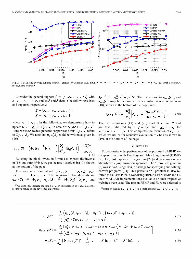
Fig. 2. NMSE and average runtime versus graphs for Gaussian-i.i.d. input. , , , . (a) NMSE versus .(b) Runtime versus .

Consider the general support withand let and denote the following subset

and superset, respectively:

where . In the following, we demonstrate how to

update to obtain10 .Here, we use to designate the supports and thus refersto . We note that could be written as given in(16).

(16)By using the block inversion formula to express the inverse

of (16) and simplifying, we get the result as given in (17), shownat the bottom of the page.

This recursion is initialized byfor . The recursion also depends on

, and

10We explicitly indicate the size of in this notation as it elucidates therecursive nature of the developed algorithms.

. The recursions for , andmay be determined in a similar fashion as given in

(18), shown at the bottom of the page, and11

(20)

The two recursions (18) and (20) start at andare thus initialized by and for

. This completes the recursion ofwhich we utilize for recursive evaluation of as shown in(19), at the bottom of the page.

V. RESULTS

To demonstrate the performance of the proposed SABMP, wecompare it here with Fast Bayesian Matching Pursuit (FBMP)[9], [15], Fast Laplace (FL) algorithm [22] and the convex relax-ation-based -optimization approach. The problem given in(2) was solved using CVX, a package for specifying and solvingconvex programs [24]. This particular problem is also re-ferred to as Basis Pursuit Denoising (BPDN). For FBMP and FLtheir MATLAB implementations available on their respectivewebsites were used. The reason FBMP and FL were selected is

11Notation such as is a short hand for .

(17)

(18)

(19)


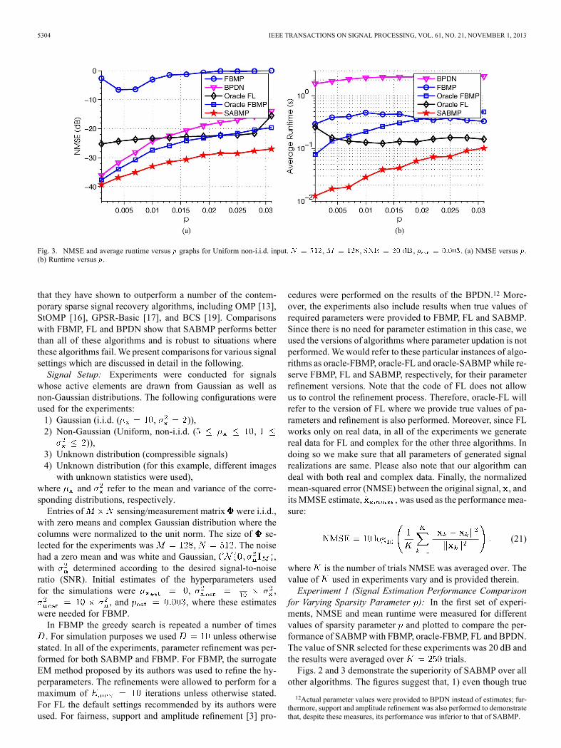
Fig. 3. NMSE and average runtime versus graphs for Uniform non-i.i.d. input. , , , . (a) NMSE versus .(b) Runtime versus .

that they have shown to outperform a number of the contem-porary sparse signal recovery algorithms, including OMP [13],StOMP [16], GPSR-Basic [17], and BCS [19]. Comparisonswith FBMP, FL and BPDN show that SABMP performs betterthan all of these algorithms and is robust to situations wherethese algorithms fail. We present comparisons for various signalsettings which are discussed in detail in the following.Signal Setup: Experiments were conducted for signals

whose active elements are drawn from Gaussian as well asnon-Gaussian distributions. The following configurations wereused for the experiments:1) Gaussian (i.i.d. ( , )),2) Non-Gaussian (Uniform, non-i.i.d. ( ,

)),3) Unknown distribution (compressible signals)4) Unknown distribution (for this example, different imageswith unknown statistics were used),

where and refer to the mean and variance of the corre-sponding distributions, respectively.Entries of sensing/measurement matrix were i.i.d.,

with zero means and complex Gaussian distribution where thecolumns were normalized to the unit norm. The size of se-lected for the experiments was , . The noisehad a zero mean and was white and Gaussian, ,with determined according to the desired signal-to-noiseratio (SNR). Initial estimates of the hyperparameters usedfor the simulations were , ,

, and , where these estimateswere needed for FBMP.In FBMP the greedy search is repeated a number of times. For simulation purposes we used unless otherwise

stated. In all of the experiments, parameter refinement was per-formed for both SABMP and FBMP. For FBMP, the surrogateEM method proposed by its authors was used to refine the hy-perparameters. The refinements were allowed to perform for amaximum of iterations unless otherwise stated.For FL the default settings recommended by its authors wereused. For fairness, support and amplitude refinement [3] pro-

cedures were performed on the results of the BPDN.12 More-over, the experiments also include results when true values ofrequired parameters were provided to FBMP, FL and SABMP.Since there is no need for parameter estimation in this case, weused the versions of algorithms where parameter updation is notperformed. We would refer to these particular instances of algo-rithms as oracle-FBMP, oracle-FL and oracle-SABMPwhile re-serve FBMP, FL and SABMP, respectively, for their parameterrefinement versions. Note that the code of FL does not allowus to control the refinement process. Therefore, oracle-FL willrefer to the version of FL where we provide true values of pa-rameters and refinement is also performed. Moreover, since FLworks only on real data, in all of the experiments we generatereal data for FL and complex for the other three algorithms. Indoing so we make sure that all parameters of generated signalrealizations are same. Please also note that our algorithm candeal with both real and complex data. Finally, the normalizedmean-squared error (NMSE) between the original signal, , andits MMSE estimate, , was used as the performance mea-sure:

(21)

where is the number of trials NMSE was averaged over. Thevalue of used in experiments vary and is provided therein.Experiment 1 (Signal Estimation Performance Comparison

for Varying Sparsity Parameter ): In the first set of experi-ments, NMSE and mean runtime were measured for differentvalues of sparsity parameter and plotted to compare the per-formance of SABMPwith FBMP, oracle-FBMP, FL and BPDN.The value of SNR selected for these experiments was 20 dB andthe results were averaged over trials.Figs. 2 and 3 demonstrate the superiority of SABMP over all

other algorithms. The figures suggest that, 1) even though true

12Actual parameter values were provided to BPDN instead of estimates; fur-thermore, support and amplitude refinement was also performed to demonstratethat, despite these measures, its performance was inferior to that of SABMP.


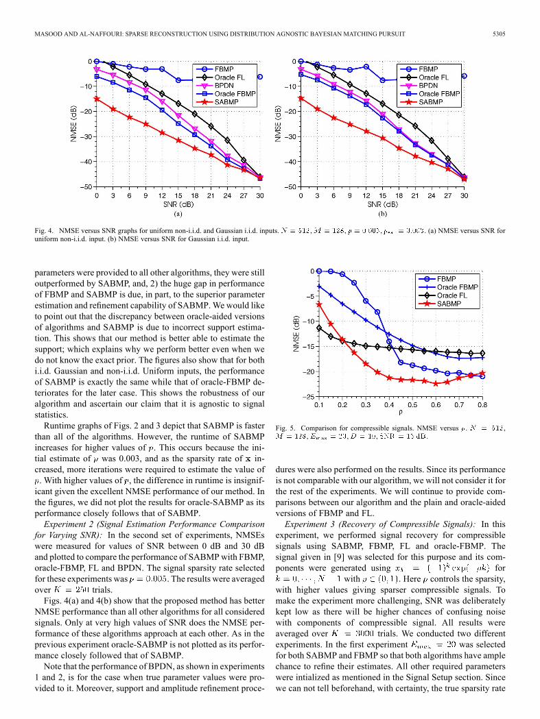
Fig. 4. NMSE versus SNR graphs for uniform non-i.i.d. and Gaussian i.i.d. inputs. , , , . (a) NMSE versus SNR foruniform non-i.i.d. input. (b) NMSE versus SNR for Gaussian i.i.d. input.

parameters were provided to all other algorithms, they were stilloutperformed by SABMP, and, 2) the huge gap in performanceof FBMP and SABMP is due, in part, to the superior parameterestimation and refinement capability of SABMP.We would liketo point out that the discrepancy between oracle-aided versionsof algorithms and SABMP is due to incorrect support estima-tion. This shows that our method is better able to estimate thesupport; which explains why we perform better even when wedo not know the exact prior. The figures also show that for bothi.i.d. Gaussian and non-i.i.d. Uniform inputs, the performanceof SABMP is exactly the same while that of oracle-FBMP de-teriorates for the later case. This shows the robustness of ouralgorithm and ascertain our claim that it is agnostic to signalstatistics.Runtime graphs of Figs. 2 and 3 depict that SABMP is faster

than all of the algorithms. However, the runtime of SABMPincreases for higher values of . This occurs because the ini-tial estimate of was 0.003, and as the sparsity rate of in-creased, more iterations were required to estimate the value of. With higher values of , the difference in runtime is insignif-icant given the excellent NMSE performance of our method. Inthe figures, we did not plot the results for oracle-SABMP as itsperformance closely follows that of SABMP.Experiment 2 (Signal Estimation Performance Comparison

for Varying SNR): In the second set of experiments, NMSEswere measured for values of SNR between 0 dB and 30 dBand plotted to compare the performance of SABMPwith FBMP,oracle-FBMP, FL and BPDN. The signal sparsity rate selectedfor these experiments was . The results were averagedover trials.Figs. 4(a) and 4(b) show that the proposed method has better

NMSE performance than all other algorithms for all consideredsignals. Only at very high values of SNR does the NMSE per-formance of these algorithms approach at each other. As in theprevious experiment oracle-SABMP is not plotted as its perfor-mance closely followed that of SABMP.Note that the performance of BPDN, as shown in experiments

1 and 2, is for the case when true parameter values were pro-vided to it. Moreover, support and amplitude refinement proce-

Fig. 5. Comparison for compressible signals. NMSE versus . ,, , , .

dures were also performed on the results. Since its performanceis not comparable with our algorithm, we will not consider it forthe rest of the experiments. We will continue to provide com-parisons between our algorithm and the plain and oracle-aidedversions of FBMP and FL.Experiment 3 (Recovery of Compressible Signals): In this

experiment, we performed signal recovery for compressiblesignals using SABMP, FBMP, FL and oracle-FBMP. Thesignal given in [9] was selected for this purpose and its com-ponents were generated using for

with . Here controls the sparsity,with higher values giving sparser compressible signals. Tomake the experiment more challenging, SNR was deliberatelykept low as there will be higher chances of confusing noisewith components of compressible signal. All results wereaveraged over trials. We conducted two differentexperiments. In the first experiment was selectedfor both SABMP and FBMP so that both algorithms have amplechance to refine their estimates. All other required parameterswere intialized as mentioned in the Signal Setup section. Sincewe can not tell beforehand, with certainty, the true sparsity rate


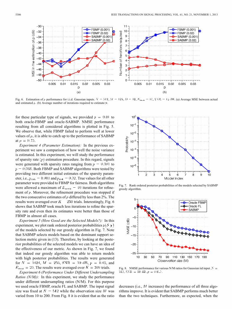
Fig. 6. Estimation of performance for i.i.d. Gaussian inputs. , , , , . (a) Average MSE between actualand estimated . (b) Average number of iterations required to estimate .

for these particular type of signals, we provided toboth oracle-FBMP and oracle-SABMP. NMSE performanceresulting from all considered algorithms is plotted in Fig. 5.We observe that, while FBMP failed to perform well at lowervalues of , it is able to catch up to the performance of SABMPat .Experiment 4 (Parameter Estimation): In the previous ex-

periment we saw a comparison of how well the noise varianceis estimated. In this experiment, we will study the performanceof sparsity rate estimation procedure. In this regard, signalswere generated with sparsity rates ranging from to

. Both FBMP and SABMP algorithms were tested byproviding two different initial estimates of the sparsity param-eter, i.e., and . True values for all otherparameter were provided to FBMP for fairness. Both algorithmswere allowed a maximum of iterations for refine-ment of . Moreover, the refinement procedure was stopped ifthe two consecutive estimates of differed by less than 2%. Theresults were averaged over trials. Interestingly, Fig. 6shows that SABMP took much less iterations to refine the spar-sity rate and even then its estimates were better than those ofFBMP in almost all cases.Experiment 5 (How Good are the Selected Models?): In this

experiment, we plot rank ordered posterior probabilitiesof the models selected by our greedy algorithm in Fig. 7. Notethat SABMP selects models based on the dominant support se-lection metric given in (13). Therefore, by looking at the poste-rior probabilities of the selected models we can have an idea ofthe effectiveness of our metric. As shown in Fig. 7, we foundthat indeed our greedy algorithm was able to return modelswith high posterior probabilities. The results were generatedfor , , , , and

. The results were averaged over trials.Experiment 6 (Performance Under Different Undersampling

Ratios (N/M)): In this experiment, we study the performanceunder different undersampling ratios (N/M). For this purposewe used oracle FBMP, oracle FL and SABMP. The input signalsize was fixed at while the observation size wasvaried from 10 to 200. From Fig. 8 it is evident that as the ratio

Fig. 7. Rank ordered posterior probabilities of the models selected by SABMPgreedy algorithm.

Fig. 8. NMSE performance for various N/M ratios for Gaussian iid input., , .

decreases (i.e., increases) the performance of all three algo-rithms improve. It is evident that SABMP performs much betterthan the two techniques. Furthermore, as expected, when the


Fig. 9. SABMP performance for Gaussian, Laplacian and Uniform noise. , , . (a) NMSE versus sparsity rate . .(b) NMSE versus SNR. .

number of observations decreased the performance of all algo-rithms deteriorated. trials were performed to generatethe graphs.Experiment 7 (Performance Under Non-Gaussian Noise As-

sumption): In this experiment, we study the performance ofSABMPwhen the assumption of Gaussian noise is not valid.Weperformed this experiment for the Laplacian and Uniform noiseand compared it with the Gaussian noise case. Noise were con-sidered to be zero-mean and the noise power adjusted accordingto the desired SNR. Fig. 9(a) shows the performance for varyingsparsity rate . In this case the SNR was kept at 20 dB. Simi-larly, in Fig. 9(b), a comparison is performed for varying SNRwhile the sparsity rate was fixed at 0.015. Both figures showthat the performance is same irrespective of the noise distribu-tion and thus highlight the robustness of SABMP against noisedistribution.Experiment 8 (Comparison of Multiscale Image Recovery

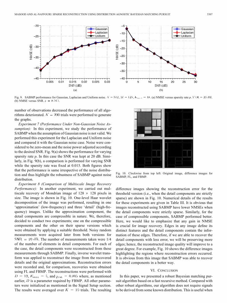
Performance): In another experiment, we carried out mul-tiscale recovery of Mondrian image of 128 128 pixels insize. The image is shown in Fig. 10. One-level Haar waveletdecomposition of the image was performed, resulting in one‘approximation’ (low-frequency) and three ‘detail’ (high-fre-quency) images. Unlike the approximation component, thedetail components are compressible in nature. We, therefore,decided to conduct two experiments; one on the compressiblecomponents and the other on their sparse versions whichwere obtained by applying a suitable threshold. Noisy randommeasurements were acquired later from both versions for

. The number of measurements taken were 1/4of the number of elements in detail components. For each ofthe case, the detail components were reconstructed from thesemeasurements through SABMP. Finally, inverse wavelet trans-form was applied to reconstruct the image from the recovereddetails and the original approximations. Reconstruction errorswere recorded and, for comparison, recoveries were obtainedusing FL and FBMP. The reconstructions were performed with

, , and where, as mentionedearlier, is a parameter required by FBMP. All other parame-ters were initialized as mentioned in the Signal Setup section.The results were averaged over trials. The resulting

Fig. 10. Clockwise from top left: Original image, difference images forSABMP, FL, and FBMP.

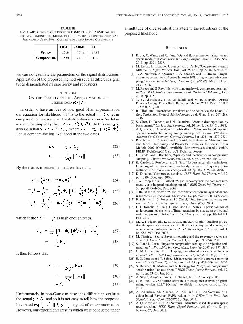
difference images showing the reconstruction error for thethreshold version (i.e., when the detail components are strictlysparse) are shown in Fig. 10. Numerical details of the resultsfor these experiments are given in Table III. It is obvious thatimages reconstructed using SABMP have lower NMSEs whenthe detail components were strictly sparse. Similarly, for thecase of compressible components, SABMP performed better.Here, we would like to emphasize that any gain in NMSEis crucial for image recovery. Edges in any image define itsdistinct features and the detail components contain the infor-mation of these edges. Therefore, if we are able to recover thedetail components with less error, we will be preserving moreedges; hence, the reconstructed image quality will improve to agreat degree. For example, Fig. 10 shows the difference imageshighlighting the regions where reconstruction errors occurred.It is obvious from this image that SABMP was able to recoverthe detail components in a better way.

VI. CONCLUSION

In this paper, we presented a robust Bayesian matching pur-suit algorithm based on a fast recursive method. Compared withother robust algorithms, our algorithm does not require signalsto be derived from some known distribution. This is useful when


TABLE IIINMSE (dB) COMPARISONS BETWEEN FBMP, FL AND SABMP FOR THETEST IMAGE (MONDRIAN) SHOWN IN FIG. 10 WHEN RECONSTRUCTION WASPERFORMED USING BOTH COMPRESSIBLE AND SPARSE COMPONENTS

we can not estimate the parameters of the signal distributions.Application of the proposed method on several different signaltypes demonstrated its superiority and robustness.

APPENDIXON THE QUALITY OF THE APPROXIMATION OF

LIKELIHOOD

In order to have an idea of how good of an approximationour equation for likelihood (11) is to the actual , let uscompare it to the case when the distribution is known. So, let usassume for simplicity that . In this case isalso Gaussian , where .Let us compare the log likelihood in the two cases

(22)

(23)

By the matrix inversion lemma, we have that

(24)

(25)

(26)

which if the is high enough reads,

(27)

(28)

It thus follows that

(29)

(30)

(31)

Unfortunately in non-Gaussian case it is difficult to evaluatethe actual and so it is not easy to tell how the proposed

likelihood is good of an approximation.However, our experimental results which were conducted under

a multitude of diverse situations attest to the robustness of theproposed likelihood.

REFERENCES

[1] K. Jia, X. Wang, and X. Tang, “Optical flow estimation using learnedsparse model,” in Proc. IEEE Int. Conf. Comput. Vision (ICCV), Nov.2011, pp. 2391–2398.

[2] M. Lustig, D. Donoho, J. Santos, and J. Pauly, “Compressed sensingMRI,” IEEE Signal Process. Mag., vol. 25, no. 2, pp. 72–82,Mar. 2008.

[3] T. Al-Naffouri, A. Quadeer, F. Al-Shaalan, and H. Hmida, “Impul-sive noise estimation and cancellation in DSL using compressive sam-pling,” in Proc. IEEE Int. Symp. Circuits Syst. (ISCAS), May 2011, pp.2133–2136.

[4] M. Firooz and S. Roy, “Network tomography via compressed sensing,”in Proc. IEEE Global Telecommun. Conf. (GLOBECOM 2010), Dec.2010, pp. 1–5.

[5] T. Y. Al-Naffouri, E. B. Al-Safadi, and M. E. Eltayeb, “OFDMPeak-to-Average Power Ratio Reduction Method,” U.S. Patent 2011/0122 930, May 2011.

[6] R. Tibshirani, “Regression shrinkage and selection via the Lasso,” J.Roy. Statist. Soc. Series B-Methodological, vol. 58, no. 1, pp. 267–288,1996.

[7] S. Chen, D. Donoho, and M. Saunders, “Atomic decomposition bybasis pursuit,” SIAM J. Sci. Comput., vol. 20, no. 1, pp. 33–61, 1998.

[8] A. Quadeer, S. Ahmed, and T. Al-Naffouri, “Structure based bayesiansparse reconstruction using non-gaussian prior,” in Proc. 49th Annu.Allerton Conf. Commun., Control, Comput., Sep. 2011, pp. 277–283.

[9] P. Schniter, L. C. Potter, and J. Ziniel, Fast Bayesian Matching Pur-suit: Model Uncertainty and Parameter Estimation for Sparse LinearModels 2009 [Online]. Available: http://www.ece.osu.edu/~zinielj/FBMP_TechRep.pdf, OSU ECE Technical Report

[10] E. Candes and J. Romberg, “Sparsity and incoherence in compressivesampling,” Inverse Problems, vol. 23, no. 3, pp. 969–985, Jun. 2007.

[11] E. Candes, J. Romberg, and T. Tao, “Robust uncertainty principles:Exact signal reconstruction from highly incomplete frequency infor-mation,” IEEE Trans. Inf. Theory, vol. 52, pp. 489–509, Feb. 2006.

[12] D. Donoho, “Compressed sensing,” IEEE Trans. Inf. Theory, vol. 52,pp. 1289–1306, Apr. 2006.

[13] J. A. Tropp and A. C. Gilbert, “Signal recovery from random measure-ments via orthogonal matching pursuit,” IEEE Trans. Inf. Theory, vol.53, pp. 4655–4666, Dec. 2007.

[14] J. Haupt and R. Nowak, “Signal reconstruction from noisy random pro-jections,” IEEE Trans. Inf. Theory, vol. 52, pp. 4036–4048, Sep. 2006.

[15] P. Schniter, L. C. Potter, and J. Ziniel, “Fast bayesian matching pur-suit,” in Proc. Workshop Inform. Theory Appl. (ITA), 2008.

[16] D. L. Donoho, Y. Tsaig, I. Drori, and J.-L. Starck, “Sparse solution ofunderdetermined systems of linear equations by stagewise orthogonalmatching pursuit,” IEEE Trans. Inf. Theory, vol. 58, pp. 1094–1121,Feb. 2012.

[17] M. A. T. Figueiredo, R. D. Nowak, and S. J. Wright, “Gradient projec-tion for sparse reconstruction: Application to compressed sensing andother inverse problems,” IEEE J. Sel. Topics Signal Process., vol. 1,pp. 586–597, Dec. 2007.

[18] M. Tipping, “Sparse Bayesian learning and the relevance vector ma-chine,” J. Mach. Learning Res., vol. 1, no. 3, pp. 211–244, 2001.

[19] S. Ji and L. Carin, “Bayesian compressive sensing and projection opti-mization,” in Proc. 24th Int. Conf. Mach. Learning, 2007, pp. 377–384.

[20] C. M. Bishop and M. E. Tipping, “Variational relevance vector ma-chines,” in Proc. 16th Conf. Uncertainty Artif. Intell., 2000, pp. 46–53.

[21] E. G. Larsson and Y. Selén, “Linear regression with a sparse parametervector,” IEEE Trans. Signal Process., vol. 55, pp. 451–460, Feb. 2007.

[22] S. Babacan, R. Molina, and A. Katsaggelos, “Bayesian compressivesensing using Laplace priors,” IEEE Trans. Image Process., vol. 19,no. 1, pp. 53–63, Jan. 2010.

[23] A. Sayed, Adaptive Filters. Hoboken, NJ, USA: Wiley, 2008.[24] C. R. Inc., “CVX: Matlab software for disciplined convex program-

ming, version 1.22,” [Online]. Available: http://cvxr.com/cvx Feb.2012

[25] A. Al-Rabah, M. Masood, A. Ali, and T.Y. Al-Naffouri, “Re-ceiver-based Bayesian PAPR reduction in OFDM,” in Proc. Eur.Signal Process. Conf. (EUSIPCO), Sep. 2013.

[26] A. Quadeer and T. Y. Al-Naffouri, “Structure-based Bayesian sparsereconstruction,” IEEE Trans. Signal Process., vol. 60, no. 12, pp.6354–6367, Dec. 2012.


Mudassir Masood (S’13) received the B.E. degreefrom NED University of Engineering and Tech-nology, Karachi, Pakistan, in 2001, and the M.S.degree in electrical engineering from King Fahd Uni-versity of Petroleum and Minerals, Dhahran, SaudiArabia, in 2005. He is currently working toward thePh.D. degree in electrical engineering from KingAbdullah University of Science and Technology,Thuwal, Saudi Arabia. His research interests lie inthe areas of signal processing, compressed sensingand its applications.

Mr. Masood is the recipient of a Best Student Poster Award at the ICCSPA2013 and the KAUST Fellowship and Academic Excellence Award in 2010.

Tareq Y. Al-Naffouri (M’10) received the B.S.degree in mathematics and electrical engineering(with first honors) from King Fahd University ofPetroleum and Minerals, Dhahran, Saudi Arabia, in1994, the M.S. degree in electrical engineering fromthe Georgia Institute of Technology, Atlanta, GA,USA, in 1998, and the Ph.D. degree in electricalengineering from Stanford University, Stanford, CA,USA, in 2004.Hewas aVisiting Scholar at the California Institute

of Technology, Pasadena, CA, USA, from January toAugust 2005 and during the summer of 2006. He was a Fulbright Scholar at theUniversity of Southern California from February to September 2008. He heldinternship positions at NEC Research Labs, Tokyo, Japan, in 1998, AdaptiveSystems Lab., University of California, Los Angeles, CA, USA, in 1999, Na-tional Semiconductor, Santa Clara, CA, USA, in 2001 and 2002, and BeceemCommunications Santa Clara, CA, USA, in 2004. He is currently an AssociateProfessor in the Electrical Engineering Department, King Fahd University ofPetroleum and Minerals, Saudi Arabia, and jointly at the Electrical EngineeringDepartment, King Abdullah University of Science and Technology. He has over80 publications in journal and conference proceedings, 9 standard contributions,and four issued and four pending patents. His research interests lie in the areas ofadaptive and statistical signal processing and their applications to wireless com-munications, seismic signal processing, and in multiuser information theory. Hehas recently been interested in compressive sensing and random matrix theoryand their applications.Dr.Al-Naffouri has been serving as an Associate Editor of IEEE

TRANSACTIONS ON SIGNAL PROCESSING since August 2013. He is the re-cipient of a Best Student Paper Award at the 2001 IEEE-EURASIP Workshopon Nonlinear Signal and Image Processing for his work on adaptive filteringanalysis, the IEEE Education Society Chapter Achievement Award in 2008,and the Al-Marai Award for innovative research in communication in 2009.

sparse reconstruction using distribution agnostic bayesian matching pursuit

Documents