spatial chaining in international comparisons of prices ... · preferable to compare the usa and...
TRANSCRIPT

Gra
zEco
nomicsPapers
–GEP
GEP 2018–03
Spatial Chaining in International
Comparisons of Prices and Real Incomes
Reza Hajargasht, Robert J. Hill, D. S. Prasada Rao, andSriram Shankar
February 2018
Department of Economics
Department of Public Economics
University of Graz
An electronic version of the paper may be downloaded
from the RePEc website: http://ideas.repec.org/s/grz/wpaper.html

Spatial Chaining in International Comparisons ofPrices and Real Incomes
Reza Hajargasht1, Robert J. Hill2, D. S. Prasada Rao3, and Sriram Shankar4
1 Swinburne Business School, Swinburne University of Technology, Australia
([email protected])2Department of Economics, University of Graz, Austria ([email protected])3School of Economics, University of Queensland, Australia ([email protected])
4ANU Centre for Social Research and Methods & Research School of Economics,
Australian National University, Australia ([email protected])
February 7, 2018
Abstract:
Multilateral international comparisons of the purchasing power of currencies and
real income often use as building blocks bilateral comparisons between all possible
pairs of countries. The standard approach in the literature weights all these bilaterals
equally. One problem with this approach is that some bilaterals are typically of lower
quality, and their inclusion therefore can undermine the integrity of the multilateral
comparison. Formulating multilateral comparisons as a graph theory problem, we
show how quality can be improved by replacing bilateral comparisons with their
shortest path spatially chained equivalents. We consider a few variants on this
approach, and illustrate these multilateral methods using data from the 2011 round
of the International Comparisons Program (ICP). Using some novel bounds criteria,
we demonstrate how spatial chaining improves the quality of the overall multilateral
comparison. (JEL: C43; E31; O47)
Keywords: International Comparisons Program (ICP); Price Index; Spatial Chain-
ing; Weighted GEKS; Graph Theory; Shortest Path; Spanning tree; Weighted
Relative Price Dissimilarity; Laspeyres-Paasche Spread; Afriat Multilateral Index;
Country-Product-Dummy (CPD) Method
Drafts of this paper have been presented at the International Comparisons of Income,
Prices and Production Conference at Princeton University, May 25-26 2017, the GGDC
25th Anniversary Conference, Groningen, 30th June 2017, and the Society for Economic
Measurement Conference at MIT, on 28th July 2017. The authors are grateful to the
Development Economics Data Group (DECDG) of the World Bank for making available
the detailed international comparison data used in the paper.

1 Introduction
International comparisons of prices and real income are used to motivate and test theories
of international trade, growth, development, and convergence. The main coordinator
of such comparisons at the global level, based on micro-level data, is the International
Comparisons Program (ICP) (see Deaton and Heston 2010). ICP is led by the World
Bank in collaboration with the Organization for Economic Cooperation and Development
(OECD), Eurostat, International Monetary Fund (IMF) and United Nations (UN). ICP
results are used in the Penn World Table (see Feenstra, Inklaar and Timmer 2015), the
World Bank’s World Development Indicators, the IMF’s World Economic Outlook, and
the UN’s Human Development Index (HDI). The World Bank uses the ICP results to
measure regional and global poverty, providing estimates of the number of people living
on less than US$1 or $2 per day, and by the World Health Organization (WHO) and
United Nations Educational, Scientific and Cultural Organization (UNESCO) to compare
expenditures on health and education respectively across countries (see Rao 2013). ICP
results are also used by the IMF when computing its special drawing rights (SDRs), which
determine member country budget contributions and voting power (see Silver 2010). Even
projections of greenhouse gas emissions rely on ICP results, since these projections depend
on both current and future estimates of global inequality (see Castles and Henderson 2004).
Since 2005, ICP uses the Gini-Elteto-Koves-Szulc (GEKS) method (see Gini 1931,
Elteto-Koves 1964, and Szulc 1964) to compare prices and real income across countries.
GEKS is also used by the OECD in its triennial comparisons (see World Bank 2008),
and by Eurostat in its annual comparisons (see Eurostat 2012). The building blocks of
the GEKS method are bilateral Fisher price index comparisons between all possible pairs
of countries. The GEKS formula then averages these Fisher indexes to obtain a set of
internally consistent (i.e. transitive) multilateral price indexes. Each bilateral comparison
is given equal weight in the GEKS transitivization formula.
156 countries participated fully in the 2011 round of ICP.1 A sample of 156 countries
yields a total of 12 090 distinct bilateral comparisons between pairs of countries. GEKS
1A number of other countries, including many Caribbean and Pacific islands, also participated in alimited way in ICP 2011 (see World Bank 2015)
1

gives equal weight to each of these in determining the overall results. Some of these 12 090
bilateral comparisons, however, are likely to be more reliable than others (see Aten and
Heston 2009). It should therefore be possible to improve on GEKS by either excluding
less reliable bilateral comparisons, or by giving greater weight to those bilaterals that are
deemed more reliable. The question is how best to do this?
When attempting to answer this question it is useful to reinterpret international
comparisons in a graph theory setting. Each country is denoted by a vertex and each
bilateral comparison by an edge connecting two vertices. In a comparison between K
countries, the minimum number of bilaterals (represented by edges) needed is K − 1
configured as a spanning tree (i.e. the K−1 edges connect the K vertices without creating
any cycles). Hill (1999) proposes a method based on minimum spanning trees (MSTs)
along these lines. Hill’s MST method, however, is too extreme in terms of the information
it discards, and is generally not robust to slight changes in the data or the distance metric
used.
What is needed is a method that lies somewhere in between the GEKS and MST
methods. More reliable bilateral comparisons should be given greater weight, but the
weighting scheme should not be as extreme as that employed by the MST method, which
effectively gives K − 1 bilaterals a weight of 1 and all others a weight of zero.
Such an “in-between” method already exists: namely the weighted-GEKS method of
Rao (1999, 2009). Rao shows that GEKS is a special case of weighted-GEKS. We show
here in section 3 that the same is true of the MST method.
The problem with weighted-GEKS is that it requires cardinal weights to be assigned
to each bilateral comparison, and it is not clear how much weight should be given to one
bilateral comparison versus another.
We show how this problem can be resolved by combining weighted-GEKS with spatial
chaining methods. Consider the question of how to compare a pair of countries? The
standard answer is that the best way is a direct bilateral comparison. One can imagine
situations, however, where indirect comparisons could be useful. For example, it might be
preferable to compare the USA and Honduras indirectly via Mexico rather than directly.
Such indirect comparisons across space are what we mean by spatial chaining.
2

In time series comparisons it is well recognized that chronological chaining can reduce
the sensitivity of the comparison to the choice of price index formula (see Diewert 2001).
For example, it is quite standard say to compare 2010 and 2015 by chaining through 2011,
2012, 2013, and 2014. No such natural ordering, though, exists for spatial comparisons.
Given a suitable distance metric, however, we show that spatial paths between pairs of
countries can be constructed that reduce the price index variance. In some cases the
shortest path is a direct comparison.
It follows that one way to potentially improve on GEKS is to replace all direct bilat-
erals by their shortest path equivalents, prior to application of the GEKS transitivization
formula. A second approach is to construct a shortest path spanning tree for each country
and then combine these spanning trees to construct a weights matrix for insertion into
the weighted-GEKS formula. We consider two different ways in which this can be done.
We also consider the Afriat multilateral index proposed by Dowrick and Quiggin (1997)
which, although different in its conception, is closely related to one of the spatial chaining
methods proposed here.
All of our shortest path methods delete the most egregious bilateral comparisons and
replace them with their shortest path equivalents, thus improving the overall quality of the
multilateral comparison. While a distance metric is still required to compute the shortest
paths, the weights in the GEKS or weighted GEKS formula emerge naturally from the
shortest paths. Hence the main weakness of weighted GEKS – the arbitrariness in the
choice of weights – is avoided.
We show that shortest path bilateral comparisons and shortest path GEKS multi-
lateral methods, based on a suitable distance metric, have desirable axiomatic properties.
We then compare GEKS, the MST method, and our three multilateral spatial chaining
methods empirically using ICP 2011 data. The sensitivity of the results to the choice of
method and distance metric is assessed. In some cases, the differences are quite substantial
and economically significant.
One further problem is developing criteria to establish which method is performing
best. We take a novel approach to this question by focusing on the bilateral comparisons
subsumed within a broader multilateral comparison, and specifying bounds for these bi-
3
laterals. In the case of ICP 2011, as was noted above, there are 12 090 such bilaterals.
The performance of each method can then be measured by counting how many of these
bilaterals subsumed within a multilateral comparison satisfy the bounds. We also consider
bounds derived from an approach developed by Afriat (1967, 1981). Using three different
sets of bounds criteria, we find that all three of our multilateral spatial chaining methods
outperform GEKS when the distance metric used to compute the shortest paths belongs
to the weighted relative price dissimilarity (WRPD) class.
The remainder of the paper is structured as follows. In section 2 we outline the GEKS
and weighted-GEKS methods. In section 3 we introduce our distance metrics, explain the
MST method and show that it is a special case of weighted GEKS. Section 4 focuses on
shortest paths and introduces our shortest path variants on GEKS and weighted GEKS.
Section 5 explains Afriat’s approach to spatial chaining, and the derivation of Afriat bounds
and the Afriat multilateral index. Section 6 applies the multilateral methods discussed in
sections 2-5 to ICP 2011 data. Our performance bounds criteria are explained in section
7, and then are used to evaluate the competing multilateral methods using the ICP 2011
data. Section 8 summarizes our main findings.
2 The GEKS and Weighted-GEKS Methods
2.1 The problem of intransitivity in multilateral comparisons
The bilateral price index literature focuses on the problem of finding the best price index
formula for measuring the difference in the price level between two time periods or countries
j and k. Henceforth we will assume that j and k denote countries. Alternative ways of
answering this question are provided by the economic approach (see Diewert 1976, 1999)
and the axiomatic approach (see Balk 1995 and Diewert 1999) to index numbers. Both end
up favoring the same formulas (Fisher, Tornqvist, Walsh and Sato-Vartia). Empirically
these formulas tend to approximate each other closely, and hence for most data sets it does
not matter much which is actually used (see Diewert 1978). Here we will focus mainly
on the Fisher price index P Fjk. Fisher, which is the geometric mean of Paasche P P
jk and
4

Laspeyres PLjk, is defined as follow:
P Fjk ≡
√P Pjk × PL
jk ≡
√√√√(∑N
n=1 pk,nqk,n∑Nn=1 pj,nqk,n
)×(∑N
n=1 pk,nqj,n∑Nn=1 pj,nqj,n
), (1)
where n = 1, . . . , N indexes the headings over which the comparison is being made (e.g.,
rice, bread, cereal, milk, etc), and pk,n denotes the price and qk,n the quantity purchased
of heading n in country k.
As soon as the comparison is extended to three or more countries (i.e., the comparison
switches from being bilateral to multilateral) we have a whole matrix of Fisher price
indexes:
F =
1 P F12 · · · P F
1K
P F21 1 · · · P F
2K
......
...
P FK1 P F
K2 · · · 1
. (2)
The lead diagonal of F consists of ones since when a country is compared with itself
the price index must equal one (i.e., Pkk = 1 for all k). All superlative price index
formulas (including Fisher and Tornqvist) satisfy the country reversal test, which states
that Pjk = 1/Pkj.2
An extra requirement of transitivity arises in multilateral comparisons: Pjl = Pjk ×Pkl, where Pjk denotes a price index comparison between countries j and k, and l denotes
a third country. It implies that direct and indirect comparisons give the same answer, as
is required to obtain an internally consistent set of multilateral results.
All bilateral price index formulas that are functions of the price and quantity vectors
of only the two countries being compared are intransitive, except in certain special cases
such as when the quantity or expenditure weights all equal one (see van Veelen 2002). One
solution to this problem is provided by the GEKS transitivization formula.
2The concept of a superlative price index is defined in Diewert (1976, 1978).
5

2.2 The GEKS Method
A number of approaches exist in the price index literature for obtaining transitive mul-
tilateral price indexes (see Balk 1996, Hill 1997, and Diewert 1999). The GEKS method
starts from the premise that the best comparison between a pair of countries is a bilateral
comparison. It alters the matrix of bilateral Fisher price indexes by the logarithmic least
squares amount necessary to impose transitivity. Algebraically, this least squares problem
can be written as follows:
minlnPj ,lnPk
I∑
j=1
I∑
k=1
(lnPk − lnPj − lnP Fj,k)2, (3)
where Pk denotes a multilateral price index for country k, and the normalization P1 = 1
is imposed. The solutions, ˆlnP j, ˆlnP k are the ordinary least squares (OLS) estimators of
lnPj, lnPk in the regression model:
lnP Fj,k = lnPk − lnPj + εj,k, (4)
where εj,k is a random error term.
The GEKS price indexes take the following form:
PGEKSk
PGEKSj
= exp(
ˆlnP k − ˆlnP j
)=
I∏
i=1
(P Fik
P Fij
)1/I
, (5)
where PGEKSk denotes the GEKS price index for country k, and i = 1, . . . , I indexes
the countries included in the multilateral comparison. While the GEKS transitivization
formula is usually applied to Fisher price indexes, it has also been applied to Tornqvist
price indexes (see Caves, Christensen, and Diewert 1982).
The GEKS formula can also be derived from a graph theoretic perspective. An
undirected graph consists of a set of vertices and edges, where each edge connects two
vertices. Some examples of undirected graphs (i.e., where the edges do not have directional
arrows) defined on a set of five vertices are shown in Figure 1. In our context, vertices
correspond to countries in the comparison, and edges to bilateral comparisons between
6

pairs of countries. A star comparison shown in Figure 1 places one country (say country
i) at the center of a star graph and then makes bilateral comparisons between all other
countries and country i. The price indexes now take the following form:
P star−ik
P star−ij
=P Fik
P Fij
, (6)
where P star−ik denotes the price index for country k obtained when country i is placed at
the center of the star.
Figure 1: Examples of Graphs
ttttt
tt t t
t
tt t t
t�����
@@@@@
@@
@@@
��
���
Star Graph Complete GraphChain Graph
It can now be seen that GEKS takes the geometric mean of K sets of star-graph
results, each having a different country at the center of the star. Since Fisher satisfies the
country reversal test, there is no need to specify directional arrows on the edges in the star
graph.
The GEKS method treats all countries symmetrically. In a comparison between K
countries there are a total of K(K−1)/2 possible bilateral comparisons. GEKS gives equal
weight to each of these bilateral comparisons when calculating the overall multilateral (i.e.,
transitive) results.
A problem with such an approach is that some bilateral comparisons are more reliable
than others. We consider in what follows some ways of dealing with this problem.
7

2.3 The Weighted-GEKS Method
The weighted-GEKS method (see Rao 1999, 2009) and Rao and Timmer (2003) gives
greater weight to those bilateral comparisons that are deemed more reliable. It is an
extension of (3) that solves a weighted version of the logarithmic least squares problem:
minlnPj ,lnPk
[K∑
j=1
K∑
k=1
wjk
(lnPk − lnPj − P F
jk
)2],
where the weights, wjk, measure the reliability of the bilateral comparison between coun-
tries j and k. This amounts to assuming that the errors are heteroscedastic as follows:
var(εjk) = σ2/wjk, for j 6= k. (7)
The choice of the weights formula is discussed in section 3. The complete matrix of weights
is denoted here by W . The matrix W is symmetric with zeros on the lead diagonal.
Also, if a particular bilateral comparison is assigned a weight of zero, in equation (7) this
comparison should be interpreted as having an infinite variance. Hence it plays no part in
the determination of the weighted-GEKS price indexes.
W =
0 w12 · · · w1K
w21 0 · · · w2K
......
...
wK1 wK2 · · · 0
(8)
The weighted-GEKS prices indexes, Pk, can be estimated using OLS once the model
has been transformed as follows:
√wjk lnP F
jk =√wjk lnPk −
√wjk lnPj + εjk. (9)
This approach is akin to an M-estimator that estimates parameters by minimizing a
weighted sum of squares irrespective of the covariance matrix of the disturbances (see
for example Wooldridge 2002, chapter 12).
8

OLS log price indexes on the transformed model are calculated as follows:
lnP2
lnP3
...
lnPK
=
∑Kj=1w2j −w23 · · · −w2K
−w32
∑Kj=1w3j · · · −w3K
......
...
−wK2 −wK3 · · · ∑Kj=1wKj
−1
−∑Kj=1w2j lnP F
2j
−∑Kj=1w3j lnP F
3j
...
−∑Kj=1wKj lnP F
Kj
.
(10)
The price index for country 1, P1, is again normalized to 1. In the case where wjk = w for
all j, k, the weighted-GEKS method reduces to the standard GEKS formula in (5).
In sections 3 and 4 we will consider some ways in which spatial chaining can be used
to determine the weights in (8).
3 Distance Metrics and Minimum-Spanning Trees
3.1 Distance metrics for measuring the reliability of bilateral
comparisons
Let Djk denote a distance metric for measuring the reliability of a bilateral comparison
between a pair of countries j and k. The smaller the value of Djk the more reliable the
bilateral comparison is deemed to be. We consider below some axioms for Djk.
A1: Djj = 0;
A2: Djk = Djk;
A3: Djk ≥ 0;
A4: Djk = 0 when pk,i = λpj,i for all i, (where λ > 0);
A5: Djk = 0 if and only if pk,i = λpj,i for all i (where λ > 0).
A1 states that if a country is compared with itself we know the result with certainty.
The price index must equal 1. A2 states that the way the countries are ordered does not
affect the reliability of the comparison. A3 states that the distance metric is bounded from
below by zero. A4 states that maximum reliability is assigned to bilateral comparisons that
satisfy the Hicks (1946) aggregation condition, while A5 states that maximum reliability
9
is assigned if and only if the Hicks (1946) aggregation condition is satisfied.
Here we focus on four distance metrics. The first is the Laspeyres-Paasche spread
defined as follows:
LPSjk ≡∣∣∣∣∣ln(PLjk
P Pjk
)∣∣∣∣∣ , (11)
where P Pjk and PL
jk are Paasche and Laspeyres price indexes defined in (1).3
The remaining three metrics are all examples of weighted relative price dissimilarity
(WRPD) measures denoted by W1, W2, and W3 (see Diewert 2002, 2009).
W1jk ≡N∑
n=1
(sj,n + sk,n
2
)(
pk,nP Fjk × pj,n
− 1
)2
+
(P Fjk × pj,npk,n
− 1
)2 , (12)
W2jk ≡N∑
n=1
{(sj,n + sk,n
2
)[(pk,n
P Fjk × pj,n
)+
(P Fjk × pj,npk,n
)− 2
]}, (13)
W3jk ≡N∑
n=1
(sj,n + sk,n
2
)[ln
(pk,n
P Tjk × pj,n
)]2 , (14)
where
sj,n =pj,nqj,n∑Kk=1 pk,nqk,n
, (15)
denotes the expenditure share of heading n in country j, and P Tjk, in (14), is the Tornqvist
price index formula defined as follows:
P Tjk ≡
N∏
n=1
(pk,npj,n
) sj,n+sk,n2
.
While in general we prefer to use Fisher over Tornqvist in the WRPD formula (since
Fisher satisfies the factor reversal test while Tornqvist does not – see for example Diewert
1976), we make an exception in W3. This is because when Tornqvist is used, W3 can
be interpreted as the weighted variance of the log price relatives. In practice, the choice
between Fisher and Tornqvist in the WRPD formulas has virtually no impact on our
3The ratio of a Laspeyres price index divided by a Paasche price index is equal to the ratio of aLaspeyres quantity index divided by a Paasche quantity index. Hence the LPS distance measure couldequally well be defined in terms of quantity indexes.
10
empirical results in sections 6 and 7.
The WRPD metrics satisfy all five axioms, while LPS violates A5. For example,
Djk = 0 under LPS when the Leontief (1936) aggregation conditions are satisfied (i.e.,
qk,i = µqj,i for all i, where µ > 0 is a scalar). Alternatively, it is possible that Djk =
0, under LPS, even when neither the Hicks or Leontief conditions are satisfied. In an
international comparisons context, the price data are generally less affected by noise than
the expenditure data. For this reason, given the objective of ranking bilateral comparisons
in terms of reliability, we give precedence to the Hicks aggregation condition. This leads
us to prefer the three WRPD metrics over LPS.
3.2 Spanning trees and minimum spanning trees (MSTs)
A spanning tree is a graph in which all the vertices are connected and only one path exists
between each pair of vertices. In our context again each vertex denotes a country, and
an edge linking two vertices a bilateral comparison between two countries. The star and
chain graphs in Figure 1 are examples of spanning trees. A spanning tree defined on K
countries contains exactly K − 1 edges. A total of KK−2 different spanning trees can be
constructed for a set of K countries. The minimum spanning tree (MST) is the one with
the minimum sum of weights on the edges, where the weights in our context are defined
as the distance metrics LPS or one of the WRPD metrics. In other words, unlike with
weighted GEKS, lower weights are desirable in this context.
The MST can be computed using Kruskal’s algorithm, which at each iteration selects
the edge with the smallest weight subject to the constraint that its inclusion in the graph
does not create a cycle.4 The selection of edges continues until K − 1 have been selected,
and the K countries are connected. The selected graph is the MST (see Kruskal 1956).
The MST therefore is invariant to monotonic transformations of the weights, and hence is
determined by the ordinal rankings of the weights on the edges.
Hill (1999) proposes LPS as a distance metric for computing the MST, and then
chains Fisher price indexes across the MST to obtain a set of multilateral price indexes.
4We assume there are no ties. In the presence of ties, the computation of the MST is more complicated.In our empirical comparison we use enough decimal places to ensure that ties do not arise.
11

3.3 Examples of MSTs
The empirical comparisons using ICP 2011 data in section 6 include 156 countries. Span-
ning trees defined on 156 countries are hard to visually interpret. As an illustrative ex-
ample, therefore, we provide here MSTs computed using the LPS and W1 metrics for a
sample of 14 countries drawn from all six participating regions in ICP 2011. The coun-
tries included are: 1 = AUS (Australia); 2 = BRA (Brazil); 3 = DEU (Germany); 4 =
IND (India); 5 = JPN (Japan); 6 = KAZ (Kazakhstan); 7 = MAR (Morocco); 8 = NGA
(Nigeria); 9 = PER (Peru); 10 = RUS (Russia); 11 = SAU (Saudi Arabia); 12 = THA
(Thailand); 13 = TZA (Tanzania); 14 = USA (United States).
The MSTs are shown in Figure 2. Only six of the 13 edges are common to both
MSTs. If the set of countries is more similar (e.g., all European) then it is probable that
the number of common links would be even lower. This example illustrates two problems
with the MST method. First, it is not very robust to changes in the distance metric. Also
Hill (1999) shows that it is not stable over time (i.e., from one cross-section to the next).
Second, some of the chain paths within the MST are long and not necessarily plausible.
Consider for example the path from Nigeria (NGA) to Saudi Arabia (SAU) under the W1
WRPD metric. It is partly for these reasons that we prefer multilateral methods derived
from shortest paths (see section 4) to MSTs.
3.4 Chaining across a spanning tree using the weighted GEKS
formula
A spanning tree defined on K countries can be represented as a symmetric weights matrix
W with zeroes on the lead diagonal, and 2(K − 1) elements that take the value one, and
the rest the value zero. For example, the matrix representation of the W1 MST in Figure
2b, denoted here by WMSTW1 , is depicted below.
Multilateral price indexes derived by chaining Fisher price indexes across a spanning
tree can be computed by inserting the spanning tree’s weights matrix (e.g. WMSTW1 ) into
the weighted GEKS formula in (10). The weighted GEKS formula therefore provides a fast
and elegant method for computing the multilateral price indexes derived from a spanning
12

Figure 2: Minimum Spanning Trees (MSTs)– 14 Country Example (ICP 2011)
(a) LPS Metric
(b) W1 WRPD Metric
tree. This idea is formalized by the following proposition.
Proposition 1: Suppose weights wjk are defined such that wjk = 1 if country j is
directly connected to country k in a spanning tree and zero otherwise. Then the indexes
obtained by chaining across the spanning tree are equal to the indexes obtained using a
weighted GEKS framework with weights wjk.
Proof : See Appendix A.
13

1 2 3 4 5 6 7 8 9 10 11 12 13 14
WMSTW1 =
1234567891011121314
0 0 0 0 1 0 0 0 0 0 0 0 0 10 0 1 0 0 0 0 0 1 0 0 0 0 00 1 0 0 1 0 0 0 0 0 0 0 0 00 0 0 0 0 0 0 0 0 0 0 1 0 01 0 1 0 0 0 0 0 0 0 0 0 0 00 0 0 0 0 0 0 0 1 0 0 0 0 00 0 0 0 0 0 0 0 0 0 0 1 0 00 0 0 0 0 0 0 0 0 0 0 0 1 00 1 0 0 0 1 0 0 0 1 0 1 0 00 0 0 0 0 0 0 0 1 0 0 0 0 00 0 0 0 0 0 0 0 0 0 0 0 0 10 0 0 1 0 0 1 0 1 0 0 0 1 00 0 0 0 0 0 0 1 0 0 0 1 0 01 0 0 0 0 0 0 0 0 0 1 0 0 0
.
3.5 The MST as a special case of weighted GEKS
Suppose that the weights in the weighted GEKS formula in (10) are calculated as follows:
wjk =
[1
rank(Djk)
]x, (16)
where rank(Djk) denotes the rank of the distance metric between countries j and k in
the overall distance matrix. For example, if Djk is the smallest element of the matrix
(excluding the lead diagonal), then Djk = 1. To simplify matters we assume in what
follows that there are no ties. The term x is a positive parameter.
Proposition 2: As x rises, the weighted-GEKS method based on the weights ma-
trix in (16) converges on the MST method defined on the distance metric Djk, or any
monotonically increasing function of Djk.
Proof : See Appendix B.
A counterintuitive implication of Proposition 2 is that it is possible to compute MST
price indexes using the weighted-GEKS formula without ever actually computing the MST.
In section 6 we compute MSTs defined on the 156 countries that participated in ICP 2011.
A value of x of 5 is sufficient in the weighted-GEKS formula to obtain a good approximation
to the MST method.
14
4 Shortest Path Methods
4.1 The shortest path between a pair of countries
In the context of an international spatial comparison, there is no natural ordering of
countries corresponding to the chronological ordering of time periods. Given the objective
of comparing countries j and k, the question is whether it is possible to find countries
that lie in some economically meaningful way between these two countries. If the bilateral
comparison is between the USA and Canada the answer is likely to be no. If, however,
the comparison is between USA and Tanzania it does seem plausible that one or more
intermediate link countries might be found that improve the comparison.
These ideas can be made more precise. Returning again to a graph theory context,
we define a path between countries j and k as a sequence of edges starting at the vertex
of country j and ending at the vertex of country k. The shortest path between a pair of
countries j and k is defined here as the path with the minimum sum of weights. No edge
or vertex appears more than once along the shortest path, when the weights on the edges
are all strictly positive. While in theory the shortest path is not necessarily unique, ties
are highly unlikely when the weights are computed to a few decimal places.
Let SPb→k denote the shortest path between countries b and k. It is calculated as
follows:
SPb→k = minj,l,...,m{Dbj +Djl + · · ·+Dmk}, (17)
where Djk denotes the weight on the edge connecting j and k. The shortest path can be
calculated using Dijkstra’s (1959) algorithm. A shortest path Fisher price index, SP (P Fbk),
is obtained by chaining along the shortest path derived from (17) as follows:
SP (P Fbk) = P F
bj × P Fjl × · · · × P F
mk. (18)
4.2 Economically meaningful distance metrics for shortest paths
Conceptually the choice of distance metric for computing shortest paths is not equivalent
to the choice of distance metric for a MST. In the case of a MST, following Kruskal’s
15
algorithm, the MST is determined purely by the ordinal ranking of the edges. In a shortest
path context, it has to be economically meaningful to sum the distance weights along a
chain path.
Consider again the chained Laspeyres-Paasche spread. As a result of the substitution
effect, Laspeyres is typically larger than Paasche. For example, Laspeyres is bigger than
Paasche for Household Consumption in 11 994 out of 12 090 bilateral comparisons in our
ICP 2011 data set. Inspection of the 96 cases where Paasche exceeds Laspeyres, these
bilaterals involve countries with lower quality data. In other words, these violations of
the standard Laspeyres greater than Paasche inequality can more likely be attributed to
noise in the data rather than income effects. Hence a case can be made for excluding these
bilateral comparisons.
The chained Laspeyres-Paasche Spread can be defined as follows:
ch(LPS)bk =
∣∣∣∣∣ln(PLbj
P Pbj
×PLjl
P Pjl
× · · · × PLmk
P Pmk
)∣∣∣∣∣ , (19)
where b and k are the two countries being compared. The chained comparison links through
the intermediate countries (j, l, . . . ,m). If we impose the restriction that each Laspeyres
price index PLjk is greater than its Paasche counterpart P P
jk, then it follows that (19) can
be rewritten as:
ch(LPS)bk = LPSbj + LPSjl + · · ·+ LPSmk. (20)
This implies that, when the LPS distance metric is used, chaining Paasche and Laspeyres
price indexes along the shortest path will minimize the chained Laspeyres-Paasche spread.
A more general result is provided in Proposition 3.
Proposition 3: Under plausible assumptions, chaining along the shortest path de-
fined on either the LPS or WRPD metrics reduces the variance of a bilateral comparison.
Proof : See Appendix C.
It follows therefore that LPS and WRPD are economically meaningful criteria for
computing shortest paths. Empirically, the WRPD metrics are more conservative than
16

LPS, in the sense that the shortest paths tend to include less edges.
4.3 Shortest path spanning trees
In a comparison between K countries, a shortest path can be computed between country k
and each of the other K − 1 countries in the comparison. Taking the union of these K − 1
shortest paths yields a shortest path spanning tree. Each country has its own shortest path
spanning tree. The shortest path spanning trees for India and Brazil for our 14 country
example based on the W1 WRPD metric are shown in Figure 3.
As can be seen in Figure 3, the shortest path between two countries is sometimes a
direct comparison. Conversely, sometimes the shortest path contains a number of inter-
mediate links. For example, the shortest path from India to Australia in Figure 3 passes
through Thailand, Peru, Brazil, and the USA.
Axiomatic properties of shortest path Fisher price indexes
Consider the following five axioms satisfied by a direct bilateral Fisher price index:
M1: Identity : P (p, p, qb, qk) = 1.
M2: Proportionality in Current Prices : P (pb, λpk, qb, qk) = λP (pb, pk, qb, qk) for λ > 0.
M2′: Inverse Proportionality in Base Period Prices : P (λpb, pk, qb, qk) = λ−1P (pb, pk, qb, qk)
for λ > 0.
M3: Commensurability : (Invariance to Changes in the Units of Measurement)
M4: Monotonicity in Current Prices : P (pb, pk, qb, qk) < P (pb, pj, qb, qk) if pk < pj.
M4′: Monotonicity in Base Prices : P (pb, pk, qb, qk) > P (pj, pk, qb, qk) if pb < pj.
M5: Factor reversal : P (pb, pk, qb, qk)× P (qb, qk, pb, pk) =∑N
n=1 pk,nqk,n/∑N
n=1 pb,nqb,n.
Proposition 4: Let prices and quantities be strictly positive for all commodities in
all countries. Then the shortest path Fisher price index defined by (18) using WRPD or
LPS as the distance metric satisfies M1-M5.
Proof : See Appendix D.
17
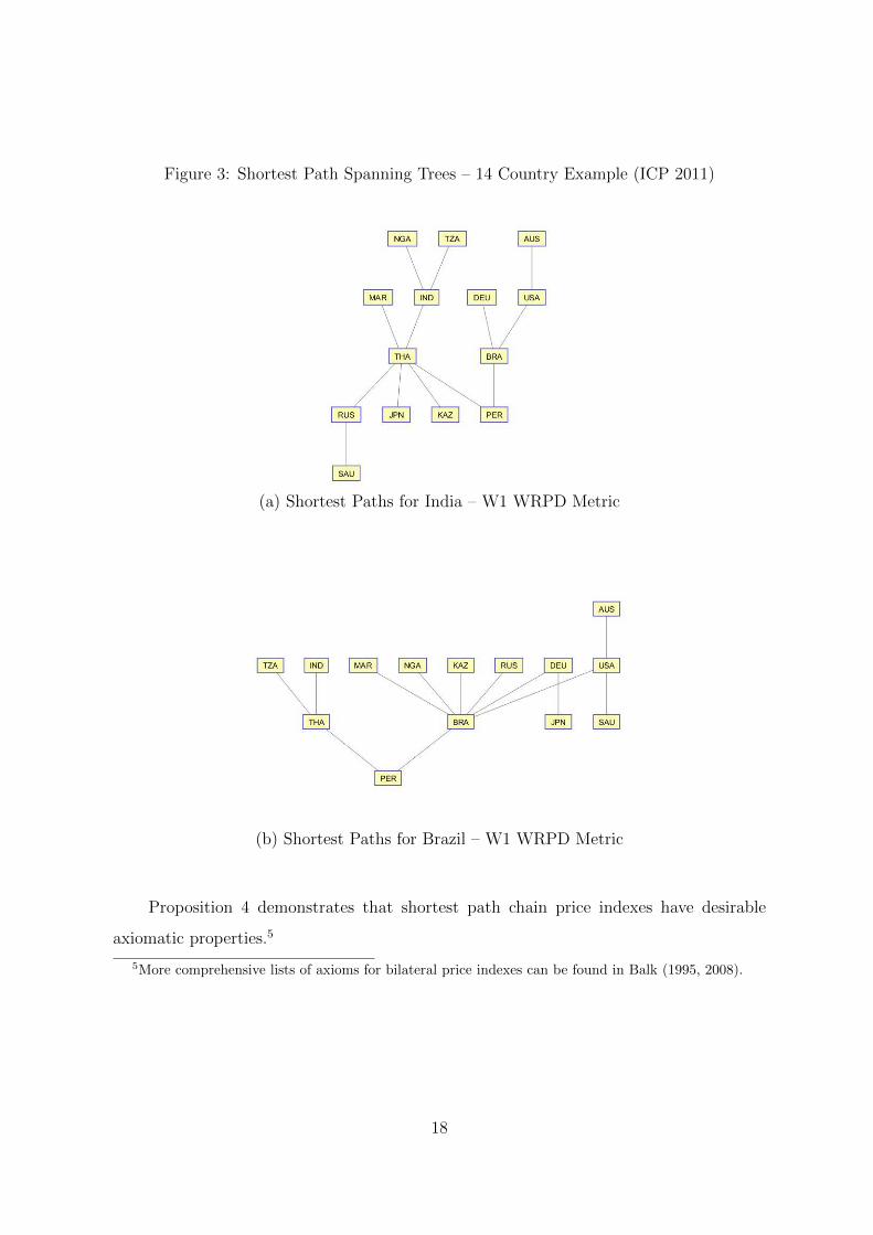
Figure 3: Shortest Path Spanning Trees – 14 Country Example (ICP 2011)
(a) Shortest Paths for India – W1 WRPD Metric
(b) Shortest Paths for Brazil – W1 WRPD Metric
Proposition 4 demonstrates that shortest path chain price indexes have desirable
axiomatic properties.5
5More comprehensive lists of axioms for bilateral price indexes can be found in Balk (1995, 2008).
18
4.4 Shortest path GEKS
Shortest path spanning trees can be used to make multilateral comparisons. The results
should be invariant to the choice of base country. Given that each country in a multilat-
eral comparison has its own shortest path spanning tree, it follows that a shortest path
multilateral method should use all the shortest path spanning trees.
All our shortest path multilateral methods are generalizations of GEKS. The first
of these methods replaces each direct Fisher in the F matrix in (2) by its shortest path
Fisher price index SP (P F ) to produce a shortest path Fisher matrix SP (F ). The GEKS
transitivization algorithm can now be applied to this shortest path Fisher matrix. This
method, therefore, replaces the most egregious direct bilaterals by shortest path chained
comparisons prior to the application of the GEKS transitivization formula.
Axiomatic properties of shortest path GEKS multilateral index
Let k = 1, . . . , K index the countries, pk and qk be vectors of the prices and quantities
for the kth country. Let P and Q be matrices containing all prices and quantities and
P (pj, pk, qj, qk) be the shortest path price index between countries j and k. Define the
associated quantity index to be
Q(pj, pk, qj, qk) =pkqk/P (pj, pk, qj, qk)
pjqj. (21)
Shortest path GEKS price and quantity indexes can be defined as follows
P kG =
∏Kj=1 P (pj, pk, qj, qk)1/K Qk
G =∏K
j=1Q(pj, pk, qj, qk)1/K
and shortest path GEKS quantity shares as
SkG =
QkG∑K
j=1QjG
. (22)
Diewert (1999) (see also Balk 1996) lists 12 test properties for multilateral indexes in terms
of quantity shares and shows that the conventional GEKS satisfies 10 of those properties.
Here we consider these 10 axioms.
T1 -Share Test : There exist K continuous, positive functions SkG(P,Q), k = 1, . . . , K such
19
that∑K
k=1 SkG(P,Q) = 1 for all P and Q in the appropriate domain of definition.
T2 -Proportional Quantities Test : Suppose that qk = βkq for some q � 0N and k =
1, . . . , K such that βk > 0 and∑K
k=1 βk = 1. Then SkG(P,Q) = βk for k = 1, . . . , K .
T3 -Proportional Prices Test : Suppose that pk = αkp for some p � 0N and αk > 0 for
k = 1, . . . , K. Then SkG(P,Q) = pqk/[p
∑Kk=1 q
k] for k = 1, . . . , K.
T4 - Commensurability Test : Let δn > 0 for n = 1, . . . , N and let ∆ denote an N by
N diagonal matrix with δn on the main diagonal. Then SkG(∆P,∆−1Q) = Sk
G(P,Q) for
k = 1, . . . , K.
T5 -Commodity Reversal Test : Let Π denote an N by N permutation matrix. Then
SkG(ΠP,ΠQ) = Sk
G(P,Q) for k = 1, . . . , K .
T6 -Country Reversal Test : Let SG(P,Q) denote a K dimensional column vector that has
the country shares S1G(P,Q), . . . , SK
G (P,Q) as components, and let Π∗ be a K by K per-
mutation matrix. Then SkG(PΠ∗, QΠ∗) = Sk
G(P,Q).
T7 -Monetary Unit Test : Let αk > 0 for k = 1, . . . , K then SkG(α1p
1, . . . , αKpK , Q) =
SkG(p1, . . . , pK , Q) for k = 1, . . . , K.
T8 -Homogeneity in Quantities Test : for i = 1, . . . , 1, let λi > 0 and let j denote another
country different from country i. Then SiG(P, q1, . . . , λiq
i, . . . , qK)/SjG(P, q1, . . . , λiq
i, . . . , qK) =
λiSiG(P,Q)/Sj
G(P,Q).
T9 -Monotonicity in Quantities Test : for each k = 1, . . . , K, SkG(P, q1, . . . , qk, . . . , qK) is
increasing in components of qk.
T10 -Bilateral Consistency in Aggregation: Let A and B be nonempty disjoint partitions
of the country indexes {1, 2, . . . , K}. Suppose that for every k ∈ A, pk = αkpa and
qk = βkqa, αk > 0, pa � 0N , q
a � 0N , βk > 0 with∑
k∈A βk = 1 and that for j ∈ B,
pj = γjpb and qj = δjq
b, γj > 0, pb � 0N , qb � 0N , δj > 0 with
∑j∈B δj = 1 . Then
∑j∈B S
jG(P,Q)/
∑k∈A S
iG(P,Q) = QF (pa, pb, qa, qb) where QF is the Fisher quantity index
defined as QF (pa, pb, qa, qb) =
√paqb
paqapbqb
pbqa.
Proposition 5: Let prices and quantities be strictly positive for all commodities in
20

all countries. Then shortest path GEKS quantity shares defined by (22) using the LPS or
WRPD distance metrics satisfy T1-T10.
Proof : See Appendix D.
Proposition 5 demonstrates that shortest path GEKS has good axiomatic properties.
4.5 Weighted-GEKS applied to the union of shortest paths
It was noted above that each country has its own shortest-path spanning tree. If we take
the union of all these shortest-path spanning trees we obtain a graph that contains cycles
(except in the special case where all the shortest path spanning trees are the same). The
union of the shortest path spanning trees, based on both the LPS and W1 WRPD metrics,
for our 14 country example are graphed in Figure 4. The union-of-shortest-paths graph in
Figure 4b for example contains 38 edges, as compared with the complete graph used by
GEKS which contains 91 edges.
The weighted-GEKS method can now be applied to this union of shortest paths graph.
Each edge that is omitted from the union of shortest paths graph is now assigned a weight
of zero, while those edges that are represented in the union of shortest paths graphs are
assigned a weight of 1.
wjk = 1 if the edge connecting countries j and k appears in at least one shortest-path
spanning tree.
wjk = 0 otherwise.
In our 14 country example, the graph in Figure 4(b) for the W1 WRPD metric can
be represented as a weights matrix. Again we use the country codes from section 3.3:
Using this weights matrix in the weighted GEKS formula in (10) yields the method
denoted here by Shortest Path Union (SP-Union). This method like the Shortest Path
GEKS method ensures that the most egregious bilaterals are removed prior to the appli-
cation of the transitivization procedure.
21

Figure 4: Union of Shortest Path Spanning Trees – 14 Country Example (ICP 2011)
(a) LPS Metric
(b) W1 WRPD Metric
22

1 2 3 4 5 6 7 8 9 10 11 12 13 14
WSP−UnionW1 =
1234567891011121314
0 0 1 0 1 0 0 0 0 0 0 0 0 10 0 1 0 0 1 1 1 1 1 0 0 0 11 1 0 0 1 0 0 0 0 0 0 0 0 10 0 0 0 0 0 0 1 0 0 0 1 1 01 0 1 0 0 1 1 1 0 1 0 1 0 00 1 0 0 1 0 0 1 1 1 1 1 0 00 1 0 0 1 0 0 1 1 1 0 1 0 00 1 0 1 1 1 1 0 1 1 1 1 1 00 1 0 0 0 1 1 1 0 1 0 1 0 00 1 0 0 1 1 1 1 1 0 1 1 0 00 0 0 0 0 1 0 1 0 1 0 0 0 10 0 0 1 1 1 1 1 1 1 0 0 1 00 0 0 1 0 0 0 1 0 0 0 1 0 01 1 1 0 0 0 0 0 0 0 1 0 0 0
.
4.6 Weighted-GEKS applied to the sum of shortest paths
An alternative weighting scheme is to count how many times each bilateral comparison
(i.e., edge) appears in the shortest path spanning trees. There is a shortest path spanning
tree for each country. Hence, given K countries, the maximum possible count for an edge
is K and the minimum is zero. The weights matrix therefore consists of integer values
ranging between 0 and K.
wjk = z where z is the number of shortest path spanning trees that contain the edge
connecting countries j and k.
This method is denoted here by Shortest Path Sum (SP-Sum). In our 14 country
example and using the same country codes as above, this method entails using the following
weights matrix in the weighted GEKS formula in (10):
When the shortest path for all bilateral comparisons is the direct comparison, then all
the shortest path spanning trees have a star configuration. The weights matrixWSP−Union
reduces to a matrix with zeroes on the lead diagonal and ones everywhere else, while the
weights matrix WSP−Sum reduces to a matrix with zeroes on the lead diagonal and the
number two everywhere else.6 It follows that under this scenario, both SP-Union and
6This latter result is observed since the edge connecting countries j and k appears in the shortest path
23

SP-Sum reduce to simple GEKS (since all edges in the weighted-GEKS formula receive
the same weight). The same is true also for SP-GEKS. In other words, all three methods
include GEKS as a special case, and only depart from GEKS when the shortest paths
between bilateral comparisons cease to be direct comparisons.
1 2 3 4 5 6 7 8 9 10 11 12 13 14
WSP−SumW1 =
1234567891011121314
0 0 2 0 5 0 0 0 0 0 0 0 0 120 0 11 0 0 4 5 5 9 5 0 0 0 122 11 0 0 4 0 0 0 0 0 0 0 0 30 0 0 0 0 0 0 2 0 0 0 12 2 05 0 4 0 0 3 2 3 0 2 0 3 0 00 4 0 0 3 0 0 3 4 2 3 3 0 00 5 0 0 2 0 0 2 3 3 0 4 0 00 5 0 2 3 3 2 0 2 2 3 2 5 00 9 0 0 0 4 3 2 0 2 0 8 0 00 5 0 0 2 2 3 2 2 0 5 5 0 00 0 0 0 0 3 0 3 0 5 0 0 0 60 0 0 12 3 3 4 2 8 5 0 0 9 00 0 0 2 0 0 0 5 0 0 0 9 0 012 12 3 0 0 0 0 0 0 0 6 0 0 0
.
5 Afriat’s Approach to Spatial Chaining
5.1 Afriat’s bounds
In a series of papers Afriat derived conditions under which a data set of prices and expen-
diture shares is consistent with the utility maximizing behavior of a representative agent
under homothetic preferences (see particularly Afriat 1967, 1981).
The starting point is the Konus (1924) cost of living index:
PK(pb, pk, u) ≡ e(pk, u)
e(pb, u),
where b and k are countries, and e(p, u) is an expenditure function measuring the mini-
mum cost of reaching the utility level u given the price vector p. When preferences are
spanning trees of countries j and k, and in none of the other shortest path spanning trees.
24

homothetic, the Konus index does not depend on the reference utility level.
PK(pb, pk) =e(pk)
e(pb),
where e(pk) ≡ e(pk, 1) is the unit expenditure function.
The Konus index is transitive when it does not depend on the reference utility level.
Under homothetic preferences it is also the case that Paasche and Laspeyres price indexes
bound the Konus index as follows:
P Pbk ≤ PK(pb, pk) ≤ PL
bk. (23)
Combining these two insights, under homotheticity, all possible Laspeyres chaining paths
between country b and country k are upper bounds on the Konus index between countries
b and k (see also Varian 1983, and Dowrick and Quiggin 1997). Similarly, all possible
Paasche chaining paths are lower bounds. Taking the minimum of the upper bounds and
the maximum of the lower bounds it will in general be possible to construct tighter bounds
on the Konus index than the direct Paasche and Laspeyres bounds in (23).
maxj,l,...,m{P PbjP
Pjl · · ·P P
mk} ≤ PK(pb, pk) ≤ minj,l,...,m{PLbjP
Ljl · · ·PL
mk}. (24)
Afriat (1981) shows that a necessary and sufficient condition for the data to be consistent
with utility maximizing behavior under homothetic preferences is that these bounds exist
(i.e., maxj,l,...,m{P PbjP
Pjl · · ·P P
mk} < minj,l,...,m{PLbjP
Ljl · · ·PL
mk}).Noting that PL
bj = 1/P Pjb , these bounds can be rewritten as follows:
1
minj,l,...,m{PLkjP
Ljl · · ·PL
mb}≤ PK(pb, pk) ≤ minj,l,...,m{PL
bjPLjl · · ·PL
mk}. (25)
Now following Dowrick and Quiggin (1997) we define Mbk as:
Mbk = minj,l,...,m{lnPLbj + lnPL
jl + · · · lnPLmk}. (26)
25

It follows from (25) that
−Mkb ≤ ln[PK(pb, pk)] ≤Mbk. (27)
To compute the upper bound in (27) a directed graph (henceforth a digraph), denoted
by G, can be constructed, where the directed edge from country b to country k has a weight
equal to ln(PLbk). The upper bound Mbk in (27) is now given by the sum of the weights
on the shortest path from country b to country k. The lower bound is the negative of the
sum of the weights on the shortest path from k to b.
Some of the weights in G are negative. However, the shortest path and Afriat bounds
exist as long as there are no negative cycles in G. A negative cycle arises when there exists
a country k such that Mkk < 0. Dijkstra’s algorithm cannot be used here to compute the
shortest paths since some of the weights are negative. The Floyd-Warshall algorithm can
be used instead. While it is slower than Dijkstra’s algorithm, it computes shortest paths
in the presence of negative weights as long as there are no negative cycles.
5.2 Afriat’s bounds as performance criteria
In section 7 we use Laspeyres-Paasche bounds and the Afriat bounds in (27) in a novel way
as a performance criterion to evaluate the performance of competing multilateral methods.
First it is necessary to determine whether there are any negative cycles in the graph
G. If so, the Afriat bounds can only be used on a subset of countries for which G does
not contain any negative cycles. The simplest case of a negative cycle is when PLbk < P P
bk
(i.e., Laspeyres is smaller than Paasche). This corresponds to lnPLbk + lnPL
kb < 0. This
situation arises for 96 of the 12 090 bilateral comparisons in the ICP data set. Hence it
follows immediately that the graph G in the case of ICP 2011 contains negative cycles.
Dowrick and Quiggin (1997) were able to find a subsample of 17 OECD countries for which
in both 1980 and 1990 there are no negative cycles in G. We are able to find a subsample
of 19 OECD countries within ICP 2011 for which a graph G can be found containing no
negative cycles. In section 7 we compute the Afriat bounds defined on all possible bilateral
pairings of these 19 countries.
26

5.3 The Afriat multilateral index
Afriat’s approach can also be used to derive a multilateral method that is related to some
of the shortest path methods proposed in section 4. The bilateral bounds in (27) are
generally not transitive. Rather, we have that Mbk ≤ Mbj + Mjk. This implies that the
indirect Afriat upper bound on the price index Pbk, obtained by chaining via country j,
is Mbj + Mjk, which in general is greater than the direct Afriat upper bound Mbk. These
bounds can be transitivized as follows:
Mbk =1
K
I∑
l=1
(Mbl −Mkl),
where l = 1, . . . , I indexes the countries in the comparison. It can be verified that Mbk =
Mbj + Mjk. Hence multilateral Afriat bounds satisfying transitivity are provided by:
−Mkb ≤ ln[PK(pb, pk)] ≤ Mbk. (28)
These bounds are not as tight as the bilateral Afriat bounds as a result of the constraints
imposed by transitivity.
Following Dowrick and Quiggin (1997), a natural choice for an Afriat type multilateral
index for country k with b as the base is
PAk
PAb
=Mbk − Mkb
2.
In general, the Afriat upper and lower bounds in (24) will be constructed from different
shortest path chains (i.e., the list of linking countries will be different). In the special case
where for each bilateral comparison the upper and lower bounds exist and use the same
chain path, the Afriat multilateral index reduces to the shortest path GEKS method with
the LPS distance metric [i.e., SP-GEKS(LPS)]. This can be seen by noting that, when the
upper and lower bounds in (27) are constructed from the same chain paths, then
1
2(Mbk −Mkb) = ln[SP (P F
bk)],
27

where SP (P Fbk) is the shortest path chained Fisher index defined in (18) based on the LPS
criterion. Applying the GEKS transitivization formula then turns (Mbk − Mkb)/2 into
(Mbk − Mkb)/2, and hence the latter corresponds to SP-GEKS(LPS).
6 An Application to ICP 2011
6.1 The country product dummy (CPD) method as a form of
spatial chaining
Each country in ICP 2011 provides price data for product categories within 155 basic
heading that together cover the components of GDP. A basic heading is the lowest level of
aggregation for which expenditure data are available from the National Accounts for each
country. Examples of basic headings include Rice, Women’s footwear, Dental services,
and Postal services. In our empirical comparisons we focus on the 110 basic headings in
Household Consumption.
Each basic heading has its own product list. For example the list for the basic
heading “Rice” could consist of Long grain rice, Jasmine rice, Basmati rice, White rice,
Medium grain, Brown rice, and Short-grained rice. To ensure the prices are comparable
across outlets and countries in ICP, the physical characteristics (e.g., the weight of the
bag of rice) and the economic characteristics (e.g., whether it is a brand) are specified.
Each country collects multiple price quotes from different locations on the products in a
heading. These are then combined to produce a product average price in each country.
The country-product-dummy (CPD) method of Summers (1973) is then used to con-
struct price indexes at basic heading level. In an ICP context the CPD method estimates
a hedonic model separately for each basic heading as follows:
ln pk,n = Dkδk +Gnγn + εk,n,
where n indexes the products within the basic heading, k the countries, and Dk and Gn
country and product dummy variables, respectively. The price index for each country for
that basic heading is obtained by exponentiating the estimated parameters on the country
28
dummy variables: pk = exp(δk). No dummy variable is included for the base country
(k = 1), and its price index p1 is normalized to 1.
A product can be included in the CPD regression when it is priced by at least two
countries. In cases where the price tableau is complete (i.e., every country prices every
product), which rarely happens in ICP, CPD generates transitive Jevons price indexes:
Pk
Pb
=N∏
n=1
(pk,npb,n
)1/N
,
where b and k are countries, and n again indexes the products in the comparison.
When there are gaps in the price tableau, things are more complicated. The bilateral
Jevons indexes are now each defined on a different mix of products, and hence they are
no longer transitive. Here we will focus on one specific case, where the product overlaps
exhibit a chain structure as shown in Figure 5. For this case, we obtain the following
result:
Proposition 6: The basic heading PPP exchange rates derived from Figure 5 using
the country product dummy (CPD) method are the same as those obtained by chaining
across a spanning tree with the countries arranged in numerical order.
Proof : See Appendix E.
When there are gaps in the price tableau, CPD combines direct Jevons indexes with
spatially chained Jevons indexes. While the example considered in Proposition 6 is very
specific, it illustrates how the CPD method, which plays such a fundamental role in ICP,
exhibits some aspects of spatial chaining.
6.2 Comparing real incomes computed using different purchas-
ing power parity (PPP) exchange rates methods
The multilateral methods compared here are listed below. We focus on the distance metrics
LPS and W1. The reason for focusing on W1 as an example of a WRPD metric is that it
performs on average slightly better than W2 and W3 in section 7.
29

Figure 5: An Overlapping Chain of Products Across Countries
• MST(LPS) = Minimum Spanning Tree using LPS metric;
• SP-GEKS(LPS) = Shortest path GEKS using LPS metric;
• SP-Union(LPS) = Shortest path union weighted GEKS using LPS metric;
• SP-Sum(LPS) = Shortest path sum weighted GEKS using LPS metric;
• MST(W1) = Minimum Spanning Tree using WRPD metric;
• SP-GEKS(W1) = Shortest path GEKS using WRPD metric;
• SP-Union(W1) = Shortest path union weighted GEKS using WRPD metric;
• SP-Sum(W1) = Shortest path sum weighted GEKS using WRPD metric;
• GEKS;
• Official ICP 2011 Results.
The purchasing power parity (PPP) exchange rates and real per capita household consump-
tion for each method are shown in Appendix G. The results for a selection of countries are
provided in Table 1.
30

Table 1: Per Capita Consumption in 2011 in US Dollars for Selected Countries
LPS SP-GEKS MST SP-Union GEKS
P.R. China 3388.1 3434.7 3303.7 3362.7Hong Kong 28642.8 28340.5 29847.5 30914.5India 2626.4 2657.5 2634.8 2664.3Australia 22207.7 21913.5 22693.7 23225.6Japan 19369.2 19164.4 19340.1 18936.7Luxembourg 24608.6 24598.4 23325.3 23829.4Ethiopia 865.6 628.2 848.6 878.1
W1 SP-GEKS MST SP-Union GEKS
P.R. China 3214.3 3284.7 3244.8 3362.7Hong Kong 29748.7 29986.2 29912.8 30914.5India 2631.3 2648.3 2608.8 2664.3Australia 22013.4 22246.4 22143.0 23225.6Japan 18766.6 19435.9 18955.7 18936.7Luxembourg 25724.1 26089.2 25821.2 23829.4Ethiopia 821.3 838.8 835.7 878.1
Source: Authors’ calculations.
Table 2 shows average differences in per capita consumption between GEKS and each
of the spatial chaining multilateral methods. For all spatial chaining methods, average per
capita consumption measured in US dollars is smaller than under GEKS, on average by
4.1 percent according to SP-Union(W1). The corresponding average absolute difference
is only slightly larger at 4.2 percent. Given we are making the comparison in US dollars,
per capita consumption for the USA by construction is the same for all methods in Table
2. Since per capita consumption in US dollars for other countries is on average higher
under GEKS, it follows that the gap between the USA per capita consumption and that
of poorer countries is bigger when spatial chaining methods are used. This relationship is
graphed in Figure 5 for the SP-Union(LPS) and SP-Union(W1) methods. It can be seen
that the difference between GEKS and the spatial chaining results decreases slightly as
per capita income rises.
The aggregate effect of these differences at the global and regional level is shown in
Table 3. Focusing on SP-Union(W1), consumption falls most in Western Asia (lower by 5.5
percent), followed by Latin America and Africa (lower by 4.9 and 4.3 percent respectively).
31

Table 2: Percentage Differences in Per Capita Consumption Relative to GEKS(with USA as Base)
Average Diff. Average Absolute Diff.
SP-GEKS(LPS) 4.90 5.59MST(LPS) 7.62 8.42SP-Union(LPS) 2.64 3.12SP-GEKS(W1) 5.61 5.72MST(W1) 4.36 4.88SP-Union(W1) 4.09 4.21
Notes: The percentage differences are calculated as follows. First, per capita consumption in US dollars is
computed for each country for each multilateral method. Then the difference or absolute difference in per
capita consumption for each multilateral method relative to GEKS is computed as follows: 100(GEKS -
PPP Method)/GEKS or 100|GEKS - PPP Method|/GEKS. The average difference across all 156 partici-
pating countries are reported above (with all countries weighted equally).
Table 3: Percentage Differences in World and Regional Consumption Relativeto GEKS (with USA as Base)
SP-GEKS(LPS) MST(LPS) SP-Union(LPS)
World consumption 2.30 3.11 1.45Africa 2.30 4.61 2.98Asia-Pacific 1.23 1.22 1.79CIS 6.49 5.67 4.25OECD-Eurostat 2.37 3.13 1.06Latin America 2.58 5.33 -0.52Western Asia 2.38 7.07 2.59
SP-GEKS(W1) MST(W1) SP-Union(W1)
World consumption 3.63 2.81 2.90Africa 4.74 3.34 4.29Asia-Pacific 3.56 2.27 3.21CIS 5.54 6.69 2.96OECD-Eurostat 2.97 2.21 2.27Latin America 6.48 5.47 4.88Western Asia 5.95 5.80 5.51
Notes: The percentage differences are calculated as follows. First, total consumption measured in US
dollars is computed for each country in US dollars using each multilateral method. Then consumption is
summed across all countries in the region. The average difference in consumption for each multilateral
method relative to GEKS is computed as follows: 100 (GEKS - PPP Method)/GEKS.
Let P ibk denote the price index for country k with b as the base country, computed
using PPP method i. The dissimilarity in the results of methods i and j can be measured
32

by:
Zij =
√√√√√ 1
K(K − 1)
K∑
b=1
K∑
k=1
(P jbk
P ibk
− 1
)2
+
(P ibk
P jbk
− 1
)2.
The Z statistic uses the same basic formula as the distance metric W1, except now that
it compares a pair of multilateral methods rather than a pair of countries. Z is essentially
a symmetric version of the more familiar root mean squared error.
Figure 6: Difference with GEKS as a Function of Per Capita Consumption
-10
-5
0
5
10
15
6 7 8 9 10 11
Pe
rce
nta
ge d
iffe
ren
ce f
rom
GEK
S
Log of per capita expenditure in US dollars
SP-Union(LPS)
-10
-5
0
5
10
15
6 7 8 9 10 11
Pe
rce
nta
ge d
iffe
ren
ce f
rom
GEK
S
Log of per capita expenditure in US dollars
SP-Union(W1)
LUX MDV
Notes: The horizontal axis is the log of real per capita income calculated using the PPP method stated
at the top of the graph. The vertical axis is the percentage differences from GEKS calculated as follows:
100(GEKS - PPP Method)/GEKS.
The matrix of Z statistics is presented in Table 4. Of particular interest is how each
method differs from the basic GEKS method. First, each WPRD is closer to GEKS than
its LPS counterpart. Second, the MST method is the most different from GEKS. Third,
the method that is closest to GEKS is SP-Union(W1). Fourth, the three shortest path
W1 methods all generate quite similar results.7
Also of interest are the results in the final column of Table 4. The official ICP 2011
results were computed separately for six regions. The six regions are OECD-Eurostat,
7The robustness of the results for each method to the deletion of a country is considered in AppendixF.
33

Latin America, Asia-Pacific, Western Asia, Africa, and the CIS).8 The results for these
regions were linked in a way that ensured that the inclusion of countries from other regions
did not affect the within-region results (see World Bank 2015). The official ICP 2011 results
in Table 4 are more similar to the three shortest path chaining W1 methods than to GEKS.
This indicates that the regional fixity requirement in ICP 2011 acts to move GEKS slightly
in the direction of spatial chaining.
Table 4: Differences in the ICP 2011 Purchasing Power Parity (PPP) ExchangeRates as Measured by the Z Statistic
A B C D E F G H I J
A 0.000 0.109 0.121 0.108 0.162 0.141 0.143 0.141 0.148 0.117B 0.109 0.000 0.069 0.025 0.110 0.093 0.094 0.092 0.096 0.168C 0.121 0.069 0.000 0.054 0.087 0.062 0.055 0.060 0.059 0.087D 0.108 0.025 0.054 0.000 0.105 0.085 0.085 0.084 0.086 0.111E 0.162 0.110 0.087 0.105 0.000 0.056 0.068 0.056 0.081 0.055F 0.141 0.093 0.062 0.085 0.056 0.000 0.032 0.011 0.051 0.067G 0.143 0.094 0.055 0.085 0.068 0.032 0.000 0.028 0.046 0.058H 0.141 0.092 0.060 0.084 0.056 0.011 0.028 0.000 0.050 0.056I 0.148 0.096 0.059 0.086 0.081 0.051 0.046 0.050 0.000 0.063J 0.117 0.168 0.087 0.111 0.055 0.067 0.058 0.056 0.063 0.000
Notes: The multilateral PPP methods are as follows: A = MST(LPS); B = SP-GEKS(LPS); C = SP-
Union(LPS); D = SP-Sum(LPS); E = MST(W1); F = SP-GEKS(W1); G = SP-Union(W1); H = SP-
Sum(W1); I = GEKS; J = Official ICP 2011 Results.
6.3 Chain paths
As a general rule, countries in the same region tend to have more similar economic struc-
tures. This tendency is reinforced in ICP 2011 by its regionalized structure. Therefore, it
is generally desirable that the shortest path between a pair of countries in the same region
stays within that region. Table 5 shows the number of shortest paths and MST paths
between pairs of countries in the same region for which this is true. For example, there are
50 participating countries in Africa in ICP 2011. This means that there are 1225 distinct
bilateral pairings of African countries. Of these, based on the LPS criterion, only 150 of
8CIS stands for Confederation of Independent States, and covers the countries of the former SovietUnion.
34

the shortest paths between pairs of African countries stay in Africa (i.e., do not involve
countries from other regions). For W1 the number of within-region shortest paths between
pairs of African countries is much higher at 564. Similar results are obtained for the other
five regions. In all cases, the number of within-region shortest paths are higher for W1.
Part of the explanation for this finding is that the W1 measure is more conservative than
LPS in the sense that it is less likely to replace a direct comparison with a chained one.
In a comparison across all shortest path spanning trees, on average 30 out of 155 of the
shortest paths are direct comparisons for W1, as compared with only 8 for LPS.
Table 5: Within and Between Region Links in Shortest Path and MinimumSpanning Trees
Total bilaterals Shortest paths without MST paths withoutLPS external countries external countriesAfrica 1225 150 29Asia Pacific 253 43 14CIS 36 6 0EU-OECD 1035 101 42Latin America 120 53 7West Asia 55 14 6W1Africa 1225 564 47Asia Pacific 253 127 22CIS 36 15 5EU-OECD 1035 324 45Latin America 120 75 12West Asia 55 22 8
As with the shortest paths, more of the MST paths stay within region for W1 than
for LPS. It is also noticeable that there are far less within-region paths in the MSTs than
in the shortest path spanning trees. This is because there is only one MST, while each
country has its own shortest path spanning tree.
It is also illuminating to consider a few actual examples of chain paths. Focusing on
the W1 metric, shortest paths and MST paths between pairs of countries are shown below.
The country codes are provided in Appendix G in Table G2. As can be seen, the MST
paths tend to be longer and less intuitive than their shortest path counterparts.
35
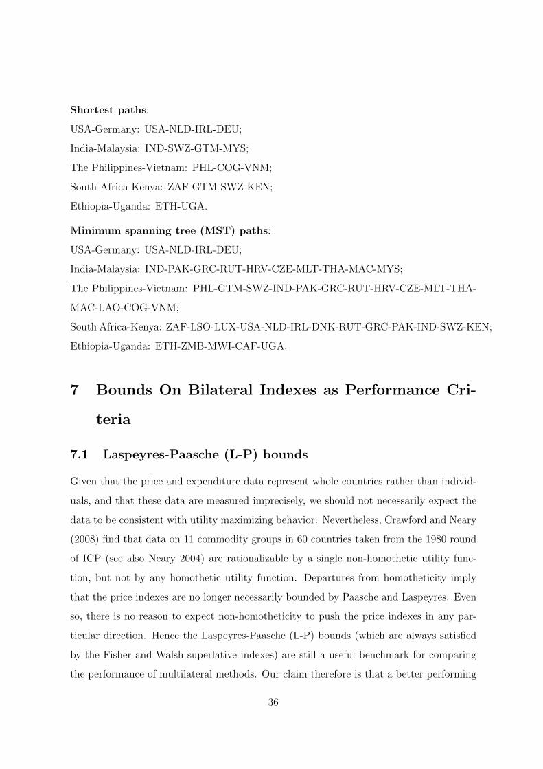
Shortest paths:
USA-Germany: USA-NLD-IRL-DEU;
India-Malaysia: IND-SWZ-GTM-MYS;
The Philippines-Vietnam: PHL-COG-VNM;
South Africa-Kenya: ZAF-GTM-SWZ-KEN;
Ethiopia-Uganda: ETH-UGA.
Minimum spanning tree (MST) paths:
USA-Germany: USA-NLD-IRL-DEU;
India-Malaysia: IND-PAK-GRC-RUT-HRV-CZE-MLT-THA-MAC-MYS;
The Philippines-Vietnam: PHL-GTM-SWZ-IND-PAK-GRC-RUT-HRV-CZE-MLT-THA-
MAC-LAO-COG-VNM;
South Africa-Kenya: ZAF-LSO-LUX-USA-NLD-IRL-DNK-RUT-GRC-PAK-IND-SWZ-KEN;
Ethiopia-Uganda: ETH-ZMB-MWI-CAF-UGA.
7 Bounds On Bilateral Indexes as Performance Cri-
teria
7.1 Laspeyres-Paasche (L-P) bounds
Given that the price and expenditure data represent whole countries rather than individ-
uals, and that these data are measured imprecisely, we should not necessarily expect the
data to be consistent with utility maximizing behavior. Nevertheless, Crawford and Neary
(2008) find that data on 11 commodity groups in 60 countries taken from the 1980 round
of ICP (see also Neary 2004) are rationalizable by a single non-homothetic utility func-
tion, but not by any homothetic utility function. Departures from homotheticity imply
that the price indexes are no longer necessarily bounded by Paasche and Laspeyres. Even
so, there is no reason to expect non-homotheticity to push the price indexes in any par-
ticular direction. Hence the Laspeyres-Paasche (L-P) bounds (which are always satisfied
by the Fisher and Walsh superlative indexes) are still a useful benchmark for comparing
the performance of multilateral methods. Our claim therefore is that a better performing
36

multilateral method should generate bilaterals that more often lie within the L-P bounds.9
As has been noted previously, a multilateral comparison between K countries contains
K(K−1)/2 distinct bilateral comparisons. Here given K = 156, we have 12 090 bilaterals.
Laspeyres exceeds Paasche for 11 994 of these. Focusing on these 11 994 bilaterals we count
the number of times the bilaterals contained within each multilateral method lie between
these L-P bounds. The results are shown in Table 6.
7.2 Geometric Laspeyres and Paasche (GL-GP) bounds
Geometric Laspeyres (GL) and geometric Paasche (GP) price indexes are defined as fol-
lows:
PGLjk ≡
N∏
n=1
(pk,npj,n
)sj,n
, PGPjk ≡
N∏
n=1
(pk,npj,n
)sk,n
,
where again sj,n and sk,n denote the expenditures shares of heading n in countries j and
k, as defined in (15).
We should necessarily expect that PGLjk > PGP
jk even under the assumption of util-
ity maximizing behavior. For example, under constant elasticity of substitution (CES)
preferences, which is larger out of PGLjk and PGP
jk depends on whether the elasticity of sub-
stitution is greater or less than one. In our data set, for about two-thirds of our bilateral
comparisons, PGLjk < PGP
jk .
GL and GP bound the Konus cost of living index when preferences are described by
the homothetic translog utility function, which is a flexible function form (see Diewert
1976). Also, GL and GP bound the superlative Tornqvist index. Again, though, in
general there is no reason to expect the bilateral price indexes subsumed within a broader
multilateral comparison to always lie within the GL and GP bounds. Indeed, the GL and
GP bounds are tighter than the Laspeyres-Paasche bounds. Nevertheless, our previous
9An alternative approach would be to estimate a demand system, which would allow Konus cost ofliving indexes to be computed for reference utility levels (see Neary 2004). One problem with such anapproach is that a demand system cannot be easily estimated for 156 countries over 110 basic headings.Typically the headings are first aggregated to a much smaller number. Oulton (2012), however, hasdeveloped an innovative method that avoids the need to aggregate headings. His method arranges thecountries in a spatial chain from poorest to richest, as measured by GEKS, and then estimates only partsof the expenditure function (primarily the income elasticities). The results, however, are sensitive to thespatial ordering of the countries, which brings us back to the theme of this paper.
37
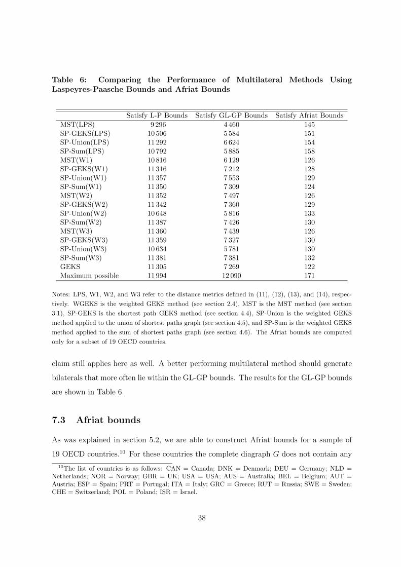
Table 6: Comparing the Performance of Multilateral Methods UsingLaspeyres-Paasche Bounds and Afriat Bounds
Satisfy L-P Bounds Satisfy GL-GP Bounds Satisfy Afriat Bounds
MST(LPS) 9 296 4 460 145SP-GEKS(LPS) 10 506 5 584 151SP-Union(LPS) 11 292 6 624 154SP-Sum(LPS) 10 792 5 885 158MST(W1) 10 816 6 129 126SP-GEKS(W1) 11 316 7 212 128SP-Union(W1) 11 357 7 553 129SP-Sum(W1) 11 350 7 309 124MST(W2) 11 352 7 497 126SP-GEKS(W2) 11 342 7 360 129SP-Union(W2) 10 648 5 816 133SP-Sum(W2) 11 387 7 426 130MST(W3) 11 360 7 439 126SP-GEKS(W3) 11 359 7 327 130SP-Union(W3) 10 634 5 781 130SP-Sum(W3) 11 381 7 381 132GEKS 11 305 7 269 122Maximum possible 11 994 12 090 171
Notes: LPS, W1, W2, and W3 refer to the distance metrics defined in (11), (12), (13), and (14), respec-
tively. WGEKS is the weighted GEKS method (see section 2.4), MST is the MST method (see section
3.1), SP-GEKS is the shortest path GEKS method (see section 4.4), SP-Union is the weighted GEKS
method applied to the union of shortest paths graph (see section 4.5), and SP-Sum is the weighted GEKS
method applied to the sum of shortest paths graph (see section 4.6). The Afriat bounds are computed
only for a subset of 19 OECD countries.
claim still applies here as well. A better performing multilateral method should generate
bilaterals that more often lie within the GL-GP bounds. The results for the GL-GP bounds
are shown in Table 6.
7.3 Afriat bounds
As was explained in section 5.2, we are able to construct Afriat bounds for a sample of
19 OECD countries.10 For these countries the complete diagraph G does not contain any
10The list of countries is as follows: CAN = Canada; DNK = Denmark; DEU = Germany; NLD =Netherlands; NOR = Norway; GBR = UK; USA = USA; AUS = Australia; BEL = Belgium; AUT =Austria; ESP = Spain; PRT = Portugal; ITA = Italy; GRC = Greece; RUT = Russia; SWE = Sweden;CHE = Switzerland; POL = Poland; ISR = Israel.
38
negative cycles. Focusing on the 171 bilaterals between these 19 countries we count the
number of times the bilaterals contained within each multilateral method lie within the
Afriat bounds. The results are also shown in Table 6.
7.4 Interpreting the bounds results
A few themes emerge from Table 6. First, the shortest path methods outperform MST
methods. Second, according to both the L-P and GL-GP bounds, shortest path methods
based on the WRPD metrics (W1, W2 and W3) outperform methods based on the LPS
metric. The reverse result is obtained for the Afriat bounds. However, the Afriat bounds
can only be computed over a sample of 19 countries, rather than the whole data set of
156 countries. Hence we attach greater importance to the L-P and GL-GP results. The
shortest path WRPD methods mostly outperform the basic GEKS method. GEKS lies
within the L-P bounds 11 305 times, and within the GL-GP bounds 7 269 times. Seven
of the nine WRPD shortest path methods achieve higher counts than GEKS for the L-P
bounds, while six out of nine achieve higher counts for the GL-GP bounds. For the Afriat
bounds, all twelve shortest path methods (i.e., LPS as well as WRPD) outperform the
GEKS count of 122.
This leaves the question of which combination of shortest path method and WRPD
metric is best. Focusing on performance relative to both the L-P and GL-GP bounds, the
best performing combination (as measured by the sum of the L-P and GL-GP counts) is
SP-Union(W1) followed by SP-Sum(W2). These methods outperform GEKS according to
all three bounds criteria.
8 Conclusion
GEKS is currently the most widely used method for making multilateral international
comparisons of prices and real incomes. GEKS starts from the assumption that the best
way to compare two countries is by a direct bilateral comparison. Transitivity is imposed
on the matrix of direct bilaterals by altering them by the least squares amount necessary to
achieve transitivity. In contrast, our starting point has been to question this assumption,
39

and consider how transitivity can be imposed instead using shortest-path methods.
To compute shortest paths, a distance metric is required. We consider Laspeyres-
Paasche spreads (LPS) and weighted-relative-price-dissimilarity (WRPD) metrics for this
purpose, and show that each can be justified in terms of minimizing the variance of the
resulting price indexes.
Spatial chaining is already used indirectly to some extent in international comparisons.
Imposing regional fixity in ICP brings in a degree of spatial chaining. Also, the country-
product-dummy (CPD) method used in ICP to construct the basic heading price indexes
can be interpreted under certain conditions as a form of spatial chaining. The Afriat
multilateral index represents another variant on spatial chaining, that is closely related to
one of our methods considered here.
Spatial chaining methods lead to significant differences in real per capita consumption
compared to GEKS. In particular, the world comes out poorer (measured in US dollars).
Based on our preferred method, total consumption falls most in Western Asia (lower by
5.5 percent), Latin America (lower by 4.9 percent) and Africa (lower by 4.3 percent). This
finding has implications for poverty analysis.
More generally, we have developed an analytical framework for constructing shortest
path spatial chains across countries, and for then using these spatial chains to make mul-
tilateral international comparisons. In terms of performance, based on three different sets
of novel bounds criteria, we find that our shortest path multilateral methods outperform
the benchmark GEKS method used by the ICP. The SP-Union method described in sec-
tion 4.6 used in combination with the W1 distance metric is our preferred shortest path
based multilateral method. SP-Union constructs the union of all shortest-path spanning
trees and assigns a weight of 1 to all edges that appear in this union, and zero other-
wise. Multilateral price indexes are then obtained by inserting this weights matrix into
the weighted-GEKS formula.
There is scope to further extend our framework, for example, to consider other ways of
constructing a weights matrix from the set of shortest path spanning trees. Other distance
metrics, and alternative performance criteria might also be used. These issues warrant
closer scrutiny. Further research notwithstanding, we have shown here that SP-Union
40

based on the W1 distance metric is a viable and attractive alternative to the widely used
GEKS method for making international comparisons of prices and real incomes.
References
Afriat, S. N. (1967), “The Construction of Utility Functions from Expenditure Data,”
International Economic Review 8, 67-77.
Afriat, S. N. (1981), “On the Constructability of Consistent Price Indices Between Several
Periods Simultaneously,” in A. Deaton, ed., Essays in the Theory and Measurement of
Consumer Behaviour. Cambridge: Cambridge University Press, 133-161.
Aten, B. and A. Heston (2009), “Are All Fishers Equal?” Mimeo.
Balk, B. M. (1995), “Axiomatic Price Index Theory: A Survey,” International Statistical
Review 63, 69-93.
Balk, B. M. (1996), “A Comparison of Ten Methods for Multilateral International Price
and Volume Comparisons,” Journal of Official Statistics 12, 199-222.
Balk, B. M. (2008), Price and Quantity Index Numbers: Models for Measuring Aggregate
Change and Difference. New York: Cambridge University Press.
Castles, I. and D. Henderson (2004), “Economics, Emissions Scenarios and the Work of the
IPCC,” Energy and Environment 14(4), 415-435.
Caves, D. W., L. R. Christensen, and W. E. Diewert (1982), “Multilateral Comparisons of
Output, Input, and Productivity Using Superlative Index Numbers,” Economic Journal
92(365), 73-86.
Crawford, I. and J. P. Neary (2008), “Testing for a Reference Consumer in International
Comparisons of Living Standards,” American Economic Review 98(4), 1731-1732.
Deaton, A. and A. Heston (2010), “Understanding PPPs and PPP-Based National Ac-
counts,” American Economic Journal: Macroeconomics 2(4), 1-35.
Diewert, W. E. (1976), “Exact and Superlative Index Numbers,” Journal of Econometrics
4, 115-145.
41

Diewert, W. E., (1978), “Superlative Index Numbers and Consistency in Aggregation,”
Econometrica 46, 883-900.
Diewert, W. E. (1999), “Axiomatic and Economic Approaches to International Compar-
isons,” in Heston, A., and R. E. Lipsey (ed.), International and Interarea Comparisons
of Income, Output and Prices, NBER, University of Chicago Press: Chicago, 13-87.
Diewert, W. E. (2001), “The Consumer Price Index and Index Number Theory: A Survey,”
Discussion Paper 01-02, Department of Economics, University of British Columbia,
Vancouver, Canada.
Diewert, W. E. (2002), “Similarity and Dissimilarity Indexes: An Axiomatic Approach,”
Discussion Paper 02-10, Department of Economics, University of British Columbia,
Vancouver, Canada.
Diewert, W. E. (2009), “Similarity Indexes and Criteria for Spatial Linking,” in Purchasing
Power Parities of Currencies: Recent Advances in Methods and Applications, D. S. P.
Rao (ed.). Edward Elgar: Cheltenham, UK, . Chapter 8, 183-216.
Dijkstra, E. W. (1959), “A Note on Two Problems in Connexion with Graphs,” Numerische
Mathematik 1, 269271.
Dowrick, S. and J. Quiggin (1997), “True Measures of GDP and Convergence,” American
Economic Review 87(1), 41-64.
Elteto, O. and P. Koves (1964), “On a Problem of Index Number Computation Relating
to International Comparison,” Statisztikai Szemle 42, 507-518.
Eurostat (2012), Eurostat-OECD Methodological Manual on Purchasing Power Parities,
Eurostat, Luxembourg.
Feenstra, R. C., R. Inklaar and M. P. Timmer (2015), “The Next Generation of the Penn
World Table,” American Economic Review 105(10), 3150-3182.
Gini, C. (1931), “On the Circular Test of Index Numbers”, International Review of Statis-
tics, Vol.9, No.2, 3-25.
Hicks, J. R., (1946), Value and Capital, Second Edition, Oxford: Clarendon Press.
42

Hill, R. J. (1997), “A Taxonomy of Multilateral Methods for Making International Com-
parisons of Prices and Quantities,” Review of Income and Wealth 43(1), 49-69.
Hill, R. J. (1999), “Comparing Price Levels Across Countries using Minimum Spanning
Trees,” Review of Economics and Statistics 81(1), 135-142
Konus, A. A. (1924), “The Problem of the True Index of the Cost of Living,” translated in
Econometrica 7 (1939), 10-29.
Kruskal, J. B. (1956), “On the Shortest Spanning Subtree of a Graph and the Travelling
Salesman Problem,” Proceedings of the American Mathematical Society 7(1), 48-50.
Leontief, W. (1936) “Composite Commodities and the Problem of Index Numbers,” Econo-
metrica 4, 39-59.
Neary, J. P. (2004), “Rationalizing the Penn World Table: True Multilateral Indices for
International Comparisons of Real Income,” American Economic Review 94(5), 1411-
1428.
Oulton, N. (2012), “The Wealth and Poverty of Nations: True PPPs for 141 Countries,”
CEP Discussion Paper No. 1080.
Rao, D. S. P. (1999), “Weighted EKS Method for Aggregation Below Basic Heading Level
Accounting for Representative Commodities,” Short Note Prepared for the ICP Unit
at the OECD.
Rao, D. S. P. (2009), “Generalised Elteto-Koves-Szulc and Country-Product-Dummy Meth-
ods for International Comparisons,” in Rao D. S. P. (ed.), Purchasing Power Parities of
Currencies: Recent Advances in Methods and Applications. Edward Elgar: Cheltenham.
Rao, D. S. P. (2013), “The Framework of the International Comparison Program,” Chapter
1 in the Measuring the Real Size of the World Economy. World Bank: Washington DC.
Rao, D. S. P. and M. Timmer (2003), “Purchasing Power Parities for Industry Comparisons
using Weighted Elteto-Koves-Szulc (EKS) Methods,” Review of Income and Wealth
49(4), 491-511.
Silver, M. (2010), “IMF Applications of Purchasing Power Parity Estimates,” IMF Working
Paper WP/10/253, International Monetary Fund. Washington DC.
43

Summers, R. (1973), “International Price Comparisons Based upon Incomplete Data,”
Review of Income and Wealth 19(1), 1-16.
Szulc, B. J. (1964), “Indices for Multiregional Comparisons”, Przeglad Statystyczny 3, Sta-
tistical Review 3, 239-254.
van Veelen, M. (2002), “An Impossibility Theorem Concerning Multilateral International
Comparison of Volumes,” Econometrica 70 (1), 369-375.
Varian, H. R. (1983), “Non-Parametric Tests of Consumer Behaviour,” Review of Economic
Studies 50(1), 99-110.
Wooldridge, J. M. (2002), Econometric Analysis of Cross Section and Panel Data. MIT
Press: Cambridge MA.
World Bank (2008), Global Purchasing Power Parities and Real Expenditures: 2005 In-
ternational Comparison Program. International Bank for Reconstruction and Develop-
ment/World Bank: Washington DC.
World Bank (2015), Purchasing Power Parities and the Real Size of World Economies: A
Comprehensive Report of the 2011 International Comparison Program. World Bank:
Washington DC.
44

Appendix For Online Publication
A: Proof of Proposition 1 in Section 3.4
We prove this proposition by induction. Suppose that we have 3 countries, without loss
of generality we can assume that the spanning tree is of the form shown in Figure A1.
Figure A1: A Spanning Tree Defined on Three Countries
1 2 3t t t
Based on this spanning tree, the indexes are defined as
lnP12 = lnP F12
lnP23 = lnP F23
lnP13 = lnP F12 + lnP F
23
(29)
where Pjk is the purchasing power parity exchange rate of country k with respect to country
j and P Fjk denotes the Fisher price index.
Weighted GEKS using the spanning tree weights is defined as follows
MinlnP1,lnP2,lnP3 Σ3j=1Σ
3k=1[wjk(lnP F
jk − lnPj + lnPk)2] (30)
where wjk = 1 if country j is directly connected to country k and zero otherwise. To see
that the indexes by chaining across the spanning tree and from weighted GEKS for the
above problem are the same, note that we can write (30) as
MinlnP1,lnP2,lnP3
{2[lnP F
12 − (lnP2 − lnP1)]2 + 2[lnP F
23 − (lnP3 − lnP2)]2}. (31)
45

Taking derivatives with respect to lnP1, lnP2 and lnP3 we can write
−2[lnP F12 − (lnP2 − lnP1)] = 0
2[lnP F12 − (lnP2 − lnP1)]− 2[lnP F
23 − (lnP3 − lnP2)] = 0
2[lnP F23 − (lnP3 − lnP2)] = 0
(32)
From the first and the last equations in (32) we have
lnP12 = lnP2 − lnP1 = lnP F12 (33)
lnP23 = lnP3 − lnP2 = lnP F23. (34)
Adding (33) and (34) results in
lnP13 = lnP3 − lnP1 = lnP F12 + lnP F
23 (35)
which proves the claim for 3 countries.
Now assume that the claim is true for any spanning tree defined on K − 1 countries,
then we can prove that the claim is true for K countries. We start with the fact that if
we have a spanning tree for K countries, there must be a country that is only connected
to one other country, and the remaining K − 1 countries are connected by a spanning tree
defined on this subset. Without loss of generality assume that this country is country-1
that is connected to country-2 and let country l be the base country. Then the equivalent
weighted GEKS indexes can be written as
MinlnP1,...,lnPK
{ΣK
j=2ΣKk=2wjk[lnP F
jk − lnPk + lnPj]2 + [lnP F
12 − lnP2 + lnP1]2}. (36)
46

Taking derivatives with respect to lnPk for k = 1, ..., K we have
−2[lnP F12 − (lnP1 − lnPl) + (lnP2 − lnPl)] = 0
∂∂ lnP2
ΣKj=2Σ
Kk=2wjk[lnP F
jk − lnPj + lnPk]2 + 2[lnP F12 − lnP2 + lnP1] = 0
∂∂ lnP3
ΣKj=2Σ
Kk=2wjk[lnP F
jk − lnPk + lnPj]2 = 0
...
∂∂ lnPK
ΣKj=2Σ
Kk=2wjk[lnP F
jk − lnPk + lnPj]2 = 0
(37)
Note that from the first equation in (37), we can write 2(lnP F12 − lnP2 + lnP1)
2 = 0.
Therefore equations 2 to K are first order conditions of the following weighted GEKS
problem (independent of lnP1).
MinlnP2,...,lnPKΣK
j=2ΣKj=2wjk[lnP F
jk − lnPk + lnPj]2 (38)
But we know that there is a path in the spanning tree that connects countries 2 to K and
therefore the claim is true for lnPl2 to lnP1N . It only remains to show that the proposition
is also true for lnP1l. Note that from the first of the first order conditions in (37) we can
write
lnP F12 − (lnP1 − lnPl) + (lnP2 − lnPl)] = 0⇒ lnPl2 = lnP F
12 (39)
which proves the proposition because country 1 is only connected to country 2 and the
claim is true for lnPl2.
B: Proof of Proposition 2 in Section 3.5
The weighted-GEKS method starts from a complete undirected graph consisting of K
vertices and K(K − 1)/2 edges, where K is the number of countries in the comparison.
Each country is represented by a vertex and a bilateral comparison between a pair of
countries by an edge. The weight on the edge connecting countries j and k is wjk. Let
the edges be ordered by the size of their weights from largest e1 to smallest eK(K−1)/2.
Suppose the edge connecting j and k has the ith largest weight. Hence ei = wjk. Given
47

the formulation of wjk in (16), it follows that:
eiei+m
=
[rank(Djk)
rank(Djk) +m
]x, where m ≥ 1 is an integer.
This ratio can be made arbitrarily small by increasing x.
Here a cycle is defined as a path that begins and ends at the same vertex and passes
through two or more edges with no repetitions of edges or vertices other than the repetition
of the starting and ending vertex. Consider now any cycle within the complete graph that
includes the edge with the smallest weight, eK(K−1)/2. By increasing x, the weight attached
to eK(K−1)/2 in the weighted-GEKS formula can be made arbitrarily small relative to that of
the other edges in that same cycle. Hence as x rises, eK(K−1)/2’s impact on the comparison
between the countries in the cycle tends to zero. The same holds for any other cycles
involving eK(K−1)/2. In the limit as x rises, therefore, the deletion of the edge with weight
eK(K−1)/2 from the graph will not affect the weighted GEKS price indexes. The same
reasoning can now be applied to the second smallest edge e(K(K−1)/2)−1, and then to the
third smallest e(K(K−1)/2)−2, etc. As long as there exists a cycle containing edge ek, and
ek is the smallest remaining edge in the graph, then in the limit as x rises edge ek can
be deleted without affecting the weighted GEKS price indexes. If ek does not appear in
any cycles then it cannot be deleted from the graph since it is required to keep all the
vertices connected. The edge with weight ek is retained, and the focus then shifts to the
next smallest edge ek−1.
Eventually a point is reached at which all cycles have been removed from the graph.
The resulting graph contains exactly K − 1 edges. For example, supposing there are 5
countries in the comparison, the outcome could be a graph with the weights matrixWA in
(40). In WA, the edge connecting countries 1 and 2 has a weight of a, the edge connecting
countries 1 and 4 has a weight of b, etc. In the weighted-GEKS formula, once there are
no longer any cycles in the graph, the weights on the remaining edges are irrelevant (as
long as they are positive). In other words, WA and WB in (40), when inserted into the
weighted-GEKS formula, will generate exactly the same price indexes, irrespective of the
48
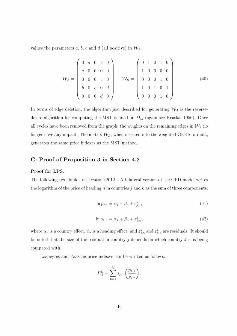
values the parameters a, b, c and d (all positive) in WA.
WA =
0 a 0 b 0
a 0 0 0 0
0 0 0 c 0
b 0 c 0 d
0 0 0 d 0
WB =
0 1 0 1 0
1 0 0 0 0
0 0 0 1 0
1 0 1 0 1
0 0 0 1 0
. (40)
In terms of edge deletion, the algorithm just described for generating WA is the reverse-
delete algorithm for computing the MST defined on Djk (again see Kruskal 1956). Once
all cycles have been removed from the graph, the weights on the remaining edges inWA no
longer have any impact. The matrixWA, when inserted into the weighted-GEKS formula,
generates the same price indexes as the MST method.
C: Proof of Proposition 3 in Section 4.2
Proof for LPS:
The following text builds on Deaton (2012). A bilateral version of the CPD model writes
the logarithm of the price of heading n in countries j and k as the sum of three components:
ln pj,n = αj + βn + εkj,n, (41)
ln pk,n = αk + βn + εjk,n, (42)
where αk is a country effect, βn is a heading effect, and εkj,n and εjk,n are residuals. It should
be noted that the size of the residual in country j depends on which country k it is being
compared with.
Laspeyres and Paasche price indexes can be written as follows:
PLjk =
N∑
n=1
sj,n
(pk,npj,n
),
49
P Pjk =
[N∑
n=1
sk,n
(pj,npk,n
)]−1,
where sj,n and sk,n are the expenditure shares of heading n in countries j and k defined in
(15). It follows from (41) and (42) that
pk,npj,n
=exp(αk) exp(εjk,n)
exp(αj) exp(εkj,n). (43)
Substituting this expression into the Laspeyres and Paasche formulas, the logarithm of the
Laspeyres-Paasche spread can be written as follows:
ln(PLjk/P
Pjk) = ln
[N∑
n=1
sj,n exp(εjk,n − εkj,n)
]+ ln
[N∑
n=1
sk,n exp(εkj,n − εjk,n)
].
Taking a second order expansion of exp(εjk,n − εkj,n) yields the following:
ln(PLjk/P
Pjk) ≈ ln
[1 +
N∑
n=1
sj,n(εkj,n − εjk,n) +N∑
n=1
sj,n(εkj,n − εjk,n)2
2
]
+ ln
[1 +
N∑
n=1
sk,n(εjk,n − εkj,n) +N∑
n=1
sk,n(εkj,n − εjk,n)2
2
]
≈ ln
[1 +
N∑
n=1
(sj,n − sk,n)(εjk,n − εkj,n) +
∑Nn=1(sj,n + sk,n)(εkj,n − εjk,n)2
2
+N∑
m=1
N∑
n=1
sj,msk,m(εkj,m − εjk,m)(εkj,n − εjk,n)
]
≈N∑
n=1
(sj,n − sk,n)(εjk,n − εjj,n) +
∑Nn=1(sj,n + sk,n)(εkj,n − εjk,n)2
2.
This same formula is derived by Deaton (2012) except that the residuals in Deaton’s
formulation are not explicitly bilateral in nature.
Taking expectations we obtain that
E[ln(PL
jk/PPjk)]≈ (σk
j )2 + (σjk)2 − 2σjk, (44)
50

where it is assumed that the errors are independently and identically distributed across
headings n.
Consider now the superlative Tornqvist price index formula:
P Tjk =
N∏
n=1
(pk,npj,n
)(sj,n+sk,n)/2
.
If we assume again the CPD price structure in (41) and (42), then
ln(P Tjk) =
[N∑
n=1
(sj,n + sk,n
2
)] [(αk − αj) + (εjk,n − εkj,n)
].
Assuming again that the errors are independently and identically distributed across
headings, the variance of the logarithm of the Tornqvist index can be written as follows:
var[ln(P Tjk)] = zjk
[(σk
j )2 + (σjk)2 − 2σjk
]= zjkE
[ln(PL
jk/PPjk)], (45)
where
zjk =
[N∑
n=1
(sj,n + sk,n
2
)2].
The variance of a chained Tornqvist index that links countries j and l via k can be
written as
var[ln(P Tjk) + ln(P T
kl)] = var(lnP Tjk) + var(lnP T
kl) + 2 cov(lnP Tjk, lnP
Tkl). (46)
Suppose the PPP-exchange rate for country k is low (e.g., the USA). In other words, one
unit of this currency has the same purchasing power as many units of other currencies. In
this case, lnPjk will tend to be negative and lnPkl positive. Conversely, when the PPP-
exchange rate for country k is high, lnPjk will tend to be positive and lnPkl negative.
It follows that the covariance term in (46) should be negative. Assuming a negative
covariance and using (45), the following sufficient condition is obtained:
zjkE[ln(PLjk/P
Pjk)]+zjkE[ln(PL
kl/PPkl )] < zjlE[ln(PL
jl/PPjl )]⇒ var[ln(P T
jk)+ln(P Tkl)] < var(lnP T
jl ).
51
There is no reason to expect any particular pattern in the z coefficients. As an approx-
imation, assuming zjk = zkl = zjl, we obtain that the chained LPS being smaller than
the direct LPS is a sufficient condition for a chained Tornqvist comparison having a lower
variance than its direct counterpart.
Proof for WRPD:
Our three weighted relative price dissimilarity (WRPD) metrics described in section 3 are
defined as follows:
W1jk =N∑
n=1
(sj,n + sk,n
2
)(
pk,nP Fjk × pj,n
− 1
)2
+
(P Fjk × pj,npk,n
− 1
)2 ,
W2jk =N∑
n=1
{(sj,n + sk,n
2
)[(pk,n
P Fjk × pj,n
)+
(P Fjk × pj,npk,n
)− 2
]},
W3jk =N∑
n=1
(sj,n + sk,n
2
)[ln
(pk,n
P Fjk × pj,n
)]2 .
Using the CPD price structure in (43), the ratio of the true price indexes αj and αk
can be approximated by a superlative price index such as Fisher or Tornqvist (see Diewert
1976, 1978). We have that
exp(αk − αj) ≈ P Fjk ≈ P T
jk.
Using Fisher as our reference, rearranging (43) yields the following expression:
pk,nP Fjk × pj,n
= exp(εjk,n − εkj,n).
Again taking a second order expansion of exp(εjk,n − εkj,n), we now obtain that
pk,nP Fjk × pj,n
− 1 ≈ (εjk,n − εkj,n) +(εjk,n − εkj,n)2
2. (47)
52

Similarly, a second order expansion of exp(εkj,n − εjk,n) yields
P Fjk × pj,npk,n
− 1 ≈ (εkj,n − εjk,n) +(εkj,n − εjk,n)2
2. (48)
Substituting (47) and (48) into the W1jk formula
W1jk ≈N∑
n=1
(sj,n + sk,n
2
)(
(εjk,n − εkj,n) +(εjk,n − εkj,n)2
2
)2
+
((εkj,n − εjk,n) +
(εkj,n − εjk,n)2
2
)2
=N∑
n=1
[(sj,n + sk,n
2
)(εjk,n − εkj,n)2 +R(3+)
],
where R(3+) denotes the sum of all terms (εjk,n − εkj,n)n for n ≥ 3. Setting R(3+) = 0, we
obtain that
W1jk ≈ 2N∑
n=1
[(sj,n + sk,n
2
)(εjk,n − εkj,n)2
]. (49)
Substituting (47) and (48) into the W2jk formula
W2jk ≈N∑
n=1
{(sj,n + sk,n
2
)[((εjk,n − εkj,n) +
(εjk,n − εkj,n)2
2
)+
((εkj,n − εjk,n) +
(εkj,n − εjk,n)2
2
)]}
=N∑
n=1
[(sj,n + sk,n
2
)(εjk,n − εkj,n)2
]. (50)
With regard to W3 for reasons that are explained in section 3 we use Tornqvist
rather than Fisher as our reference superlative price index. In addition, we make use of
the following second order approximation result:
[ln
(pk,n
P Tjk × pj,n
)]2≈[(
pk,nP Tj,n × pj,n
− 1
)− 1
2
(pk,n
P Tj,n × pj,n
− 1
)2]2.
Now using (47) it follows that
W3jk ≈N∑
n=1
(sj,n + sk,n
2
)(
(εjk,n − εkj,n) +(εjk,n − εkj,n)2
2
)− 1
2
((εkj,n − εjk,n) +
(εkj,n − εjk,n)2
2
)22 ,
53

=N∑
n=1
{(sj,n + sk,n
2
)[(εjk,n − εkj,n)2 +R(3+)]2
}.
Again setting E(3+) = 0, we obtain that
W3jk ≈N∑
n=1
[(sj,n + sk,n
2
)(εjk,n − εkj,n)2
]. (51)
Comparing (49), (50), and (51), it can be seen that
W1jk
2≈ W2jk ≈ W3jk.
This is consistent with Diewert’s (2009) finding that W1, W2, and W3 approximate each
other to the second order.
Taking expectations and comparing with (44) we obtain that
E(W1jk)
2≈ E(W2jk) ≈ E(W3jk) ≈ E
[ln(PL
jk/PPjk)]≈ (σk
j )2 + (σjk)2 − 2σjk.
Hence we obtain an expression analogous to (45). The remainder of the proof is the same
as for LPS.
D: Proofs of Axiomatic Properties of Shortest Path Indexes
Proof of Proposition 4 on the properties of shortest path Fisher price indexes
M1: Identity : P (p, p, qb, qk) = 1.
By construction, the distance metric Dbk = 0 for each of the distance metrics LPS, W1,
W2, and W3. Hence the shortest path is a direct comparison: SP (P Fbk) = P F
bk. Given that
P Fbk satisfies M1, it follows that SP (P F
bk) does likewise.
M2: Proportionality in Current Prices : P (pb, λpk, qb, qk) = λP (pb, pk, qb, qk) for λ > 0.
Define country j as having the price vector pj = λpk, and the quantity vector qj = qk.
For LPS, W1, W2, and W3 it holds that Dlj = Dlk for any country l. It follows that
the shortest path route between country b and country k will be the same as the shortest
54

path route between b and j, and hence that SP (Pbk) and SP (Pbj) will differ only in the
final bilateral price index in the chain. Let i denote the final intermediate link country in
the chain. It follows that: SPbj/SPbk = P Fij /P
Fik = λ. Again the result holds since Fisher
satisfies proportionality.
M2′: Inverse Proportionality in Base Period Prices : P (λpb, pk, qb, qk) = λ−1P (pb, pk, qb, qk)
for λ > 0.
The proof is analogous to M2.
M3: Commensurability : (Invariance to Changes in the Units of Measurement)
The distance metrics LPS, W1, W2, and W3 are all invariant to changes in the units of
measurement.
M4: Monotonicity in Current Prices : P (pb, pk, qb, qk) < P (pb, pj, qb, qk) if pk < pj.
Replacing the price vector pk with the price vector pj may cause the chain path to
change. If this happens, then monotonicity may be violated. In cases where the chain
path does not change, then M4 is satisfied. This is because, in this case, the price
indexes P (pb, pk, qb, qk) and P (pb, pj, qb, qk) will differ only in the last bilateral compari-
son in the chain. Hence the condition P (pb, pk, qb, qk) < P (pb, pj, qb, qk) is equivalent to
P F (pi, pk, qi, qk) < P F (pi, pj, qi, qk). where i is the last intermediate country in the chain.
Given that Fisher satisfies monotonicity, the shortest path price index will do likewise.
M4′: Monotonicity in Base Prices : P (pb, pk, qb, qk) > P (pj, pk, qb, qk) if pb < pj.
The proof is analogous to M4.
M5: Factor reversal : P (pb, pk, qb, qk)× P (qb, qk, pb, pk) =∑N
n=1 pk,nqk,n/∑N
n=1 pb,nqb,n.
Since Fisher satisfies M5, it follows that any chain path using Fisher also satisfies M5.
Shortest path price indexes constructed using Fisher bilateral links, therefore, satisfy
all these axioms. Monotonicity (M4 and M4′) is violated when the change in the price
vector triggers a change in the shortest path chain route.
55
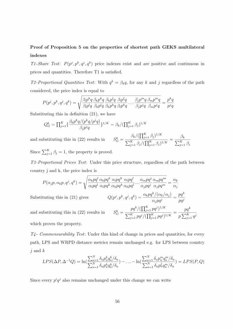
Proof of Proposition 5 on the properties of shortest path GEKS multilateral
indexes
T1 -Share Test : P (pj, pk, qj, qk) price indexes exist and are positive and continuous in
prices and quantities. Therefore T1 is satisfied.
T2 -Proportional Quantities Test : With qk = βkq, for any k and j regardless of the path
considered, the price index is equal to
P (pj, pk, qj, qk) =
√βlp
kq
βlplq
βkpkq
βkplq
βhplq
βhphq
βlplq
βlphq. . .
βjpmq
βjpjq
βmpmq
βmpjq=pkq
pjq
Substituting this in definition (21), we have
QkG =
∏Kj=1{
βkpkq/(pkq/pjq)
βjpjq}1/K = βk/(
∏Kj=1 βj)
1/K
and substituting this in (22) results in SkG =
βk/(∏K
j=1 βj)1/K
∑Kj=1 βj/(
∏Kj=1 βj)
1/K=
βk∑Kj=1 βj
Since∑K
j=1 βj = 1, the property is proved.
T3 -Proportional Prices Test : Under this price structure, regardless of the path between
country j and k, the price index is
P (αjp, αkp, qj, qk) =
√αkpq
l
αlpqlαkpq
k
αlpqkαlpq
h
αhpqhαlpq
l
αhpql....αmpq
j
αjpqjαmpq
m
αjpqm=αk
αj
Substituting this in (21) gives Q(pj, pk, qj, qk) =αkpq
k/(αk/αj)
αjpqj=pqk
pqj
and substituting this in (22) results in SkG =
pqk/(∏K
j=1 pqj)1/K
∑Kj=1 pq
j/(∏K
j=1 pqj)1/K
=pqk
p∑K
j=1 qj
which proves the property.
T4 - Commensurability Test : Under this kind of change in prices and quantities, for every
path, LPS and WRPD distance metrics remain unchanged e.g. for LPS between country
j and k
LPS(∆P,∆−1Q) = ln(
∑Nn=1 δnp
knq
hn/δn∑N
n=1 δnphnq
hn/δn
)− . . .− ln(
∑Nn=1 δnp
mn q
mn /δn∑N
n=1 δnpjnqmn /δn
) = LPS(P,Q)
Since every piqj also remains unchanged under this change we can write
56

P (∆pj,∆pk,∆−1qj,∆−1qk) = P (pj, pk, qj, qk)
Q(∆pj,∆pk,∆−1qj,∆−1qk) = Q(pj, pk, qj, qk)
and therefore SkG(∆P,∆−1Q) = Sk
G(P,Q)
T5 and T6 -Commodity Reversal Test and Country Reversal Test : These tests are satisfied
since LPS and WRPD metrics as well as chains are independent of the order of countries
or commodities.
T7 -Monetary Unit Test : Under this change in prices, for any Path, LPS and WRPD met-
rics are unchanged e.g. for LPS we have
LPSAfter = ln(αkp
kqh
αhphqh)− ln(
αkpkqk
αhphqk) + . . .+ ln(
αmpmqj
αjpjqj)− ln(
αmpmqm
αjpjqm) = LPSBefore
Therefore
P (αjpj, αkp
k, qj, qk) =
√αkp
kql
αlplqlαkp
kqk
αlplqkαlp
lqh
αhphqhαlp
lql
αhphql. . .
αmpmqj
αjpjqjαmp
mqm
αjpjqm=αk
αj
P (pj, pk, qj, qk)
Substituting in the definition (21) we have
Q(αjpj, αkp
k, qj, qk) =
αkpkqk/
αk
αj
P (pk, pj, qk, qj)
αjpjqj= Q(pj, pk, qj, qk)
Since Q(pj, pk, qj, qk) remain unchanged we must have
SkG(α1p
1, . . . , αKpK , Q) = Sk
G(p1, . . . , pK , Q)
T8 -Homogeneity in Quantities Test : First note that after this change in quantity, LPS
and WRPD metrics are unchanged since either country i is not in the chain or it is in the
chain. If it is not then clearly the chain is unaffected but even if it is, λi appears both
in numerators and denominators and will be cancelled. Similarly, for shortest path price
indexes, either country i is not in the chain or even if it is, λi will be cancelled. Therefore
Q(pj, pk, qj, qk) =pkqk/P (pj, pk, qj, qk)
pjqj= Q(pj, pk, qj, qk) if k, j 6= i
Q(pi, pk, λiqi, qk) =
pkqk/P (pi, pk, qi, qk)
λipiqi= λ−1i Q(pi, pk, qi, qk) if k 6= i
Q(pj, pi, qj, λiqi) =
λipiqi/P (pj, pi, qj, qi)
pjqj= λiQ(pj, pi, qj, qi) if j 6= i
Q(pi, pi, λiqi, λiq
i) =λip
iqi/P (pi, pi, qi, qi)
λipiqi= Q(pi, pi, qi, qi)
57

Let k = 1 and j = 2 then substituting from above in (22) and defining α = 1/∑K
j=1QjG
we can see that
S1G(P, λ1q
1, q2, . . . , qK)
S2G(P, λ1q1, q2, . . . , qK)
=α(Q(p2, p1, λ1q
1, λ1q1)∏K
j=2Q(pj, pl, λ1qj, ql))1/K
α(Q(p1, p2, λ1q1, q2)∏K
j=2Q(pj, p2, qj, q2))1/K
=(λK−1
∏Kj=1Q(pj, pl, qj, ql))1/K
(λ−1∏K
j=1Q(pj, p2, qj, q2))1/K= λ1
S1G(P,Q)
S2G(P,Q)
A similar argument can be used to prove the property for k 6= 1 and j 6= 2.
T9 -Monotonicity in Quantities Test : If the shortest path does not change after increasing
qk to q∗k we can show that
Q(pj, pk, qj, qk)
Q(pj, pk, q∗j, qk)=
pkqk
pjqj/
√pkql
plqlpkqk
plqkplqh
phqhplql
phql. . .
pmqj
pjqjpmqm
pjqm
pkq∗kpjqj
/
√pkql
plqlpkq∗kplq∗k
plqh
phqhplql
phql. . .
pmqj
pjqjpmqm
pjqm
=
√pkqk
pkq∗kplqk
plq∗k < 1
Given that QkG =
∏Kj=1Q(pj, pk, qj, qk)
1K it is easy to see that Qk
G increases with the in-
crease in components of qk. Similarly, it is possible to show that QkG is decreasing in
components of qj for j 6= k by showing
Q(pj, pk, qj, qk)
Q(pj, pk, q∗j, qk)=
√pjq∗jpjqj
pmq∗jpmqj
> 1
Given the above two facts, it can be shown that SkG = Qk
G/∑K
j=1QjG is increasing in com-
ponents of qk.
T10 -Bilateral Consistency in Aggregation: Under the conditions of this test on prices and
quantities, for any j and k irrespective of the path, the quantity index is equal to the
bilateral Fisher index (this can be checked by direct computations for any chosen path).
Given this fact, the rest of the proof is similar to the proof in Diewert (1999, see proof of
Proposition 8).
E: Proof of Proposition 6 from Section 6.1
Consider the case of K countries indexed by k = 1, . . . , K, and n = 1, . . . , N products. It
is assumed that only every adjacent pair of countries [k, k+1] shares Nk products together.
This situation is depicted in Figure 5. Let pk,n be the price of the n-th product in the
58

k-th country, Pn, the logarithm of the world average price for the n-th product and πk the
logarithm of the PPP -exchange rate of the k-th country. Then we can write the CPD
model as
ln pk,n = Pn + πk + εk,n, n = 1, . . . , N, k = 1, . . . , K. (52)
Without loss of generality, consider the K-th country as the base (which implies πK =
0). Rao and Hajargasht (2016) show that the least square estimate for P = [P1, . . . , PN ]′
and π = [π1, . . . , πK−1]′ can be obtained as
P
π
= (R′WR)−1R′W ln p
where R′ =
i′K
⊗IN
[IK−1 0K−1]⊗
i′N
, W = Diag(dkn) is an KN ×KN diagonal matrix with
dkn equal to 1 if the n-th product is priced in country k, and equal to 0 otherwise. i and 0
are column vectors of ones and zeros respectively, I is an identity matrix and⊗
denotes
the Kronecker product. Rao and Hajargasht (2016) also show that
R′WR =
K1 0 0 . . . 0... d1,1 . . . dK−1,1
0 K2 0 . . . 0... d1,2 . . . dK−1,2
0 0 0 . . . KN... d1,N . . . dK−1,N
. . . . . . . . . . . . . . . . . . . . . . . . . . . . . . . . . . . . . . . . . . . . . . . . . . . . . . . . . . . . . . . . .
d1,1 . . . d1,N... N1 0 . . . 0
d2,1 . . . d2,N... 0 N1 +N2 . . . 0
dK−1,1 . . . dK−1,N... 0 . . . NK−2 +NK−1
For definition of Nks see Figure-5 and K1 = K2 = · · · = KN = 2 given the assumed set-up
59

here. Using the formula for the inverse of partitioned matrices it can be shown that
(R′WR)−1 =
D−11 −AD−12
−D−12 A′ D−12
See Rao and Hajargasht (2016) page 421 for definition of matrices D1, D2 and A. It is
also straightforward to show that
R′W ln p =
ΣKk=1dk,1 ln pk,1
...
ΣKk=1dk,N ln pK,N
. . . . . . . . . . . . . . . . . . . .
ΣNn=1d1,n ln p1,n
...
ΣNn=1dK−1,n ln pK−1,n
Define Gj,j+1 = 1Nj
Σn∈Nj,j+1ln(
pj,npj+1,n
) as the geometric index of country j with respect to
country j + 1 where Nj,j+1 is the set of products that are priced in both country j and
j + 1. Using some tedious algebra it can be shown that for the CPD model
π1 = ΣK−1j=1 Gj,j+1 π2 = ΣK−1
j=2 Gj,j+1 ..... πK−1 = GK−1,K (53)
Note that given the way we have set-up the countries, the only possible spanning tree is
by connecting countries 1 to 2 to 3 . . . to M −1 to M and therefore based on the spanning
tree method we also have
π1 = ΣK−1j=1 Gj,j+1 π2 = ΣK−1
j=2 Gj,j+1 . . . πK−1 = GK−1,K , (54)
which proves that the indexes obtained through CPD and the spanning tree are equal for
this problem indicating that the CPD method also uses chaining while computing indexes
for countries that do not have products in common.
60

F: Robustness to country deletion – Jackknife standard errors
The robustness of a method to deletion of countries can be checked by computing Jackknife
standard errors. First, a base country b is selected. Then a country j 6= b is deleted from
the comparison, and then price indexes for the remaining K − 2 countries are computed.
Then a different country j is deleted, and price indexes are recomputed. In this way, K−2
distinct price indexes and an associated standard error can be computed for each country
k. We denote this standard error by Jbk.
Here we use the USA as the base country. The Jackknife results in Table F1 are av-
erages across all countries, where the average is computed as an arithmetic mean, median,
and geometric mean. Also shown is the standard deviation of the Jackknife estimates
for each method. Three main results emerge from Table F1. First, the results for each
method are highly skewed, as evidenced by the arithmetic means being much larger than
the medians and geometric means. This means that the results for a few countries are far
more sensitive than the rest to the deletion of countries from the comparison. Most of
these highly sensitive countries are in Africa and the Asia-Pacific regions. Second, irrespec-
tive of which average we consider, the GEKS method generates results that are the least
sensitive to the deletion of countries. The MST method is the most sensitive to country
deletion. Third, the spatial chaining methods are less sensitive to country deletion when
the distance metric W1 is used in preference to LPS. Other things equal, less sensitivity
to country deletion is desirable, although we consider the bounds criteria in section 7 to
be more important for judging the performance of multilateral methods.
Table F1: Jackknife Results
A B C D E F G H IMean 60.718 28.062 11.418 19.461 39.611 9.328 6.648 8.536 2.190Median 0.972 0.523 0.359 0.398 0.639 0.186 0.161 0.196 0.046Geomean 0.473 0.752 0.446 0.577 0.573 0.280 0.220 0.298 0.073St.Dev. 202.276 94.667 35.996 63.727 141.261 31.262 21.783 27.175 7.297
Notes: The PPP methods are again as follows: A = MST(LPS); B = Shortest path GEKS(LPS); C =
Weighted GEKS on union of shortest paths(LPS); D = Weighted GEKS on sum of shortest paths(LPS);
E = MST(W1); F = Shortest path GEKS(W1); G = Weighted GEKS on union of shortest paths(W1); H
= Weighted GEKS on sum of shortest paths(W1); I = GEKS.
61

G: PPP Exchange Rates and Real Incomes
Table G1: ICP 2011 Purchasing Power Parity (PPP) Exchange Rates forHousehold Consumption (USA=1)
A B C D E F G H I JDZA 32.70 33.14 33.98 32.84 33.96 37.11 33.00 34.51 31.80 31.77AGO 79.15 87.38 76.37 77.94 76.37 70.18 76.53 76.83 74.62 73.83BEN 246.44 258.84 233.36 241.96 237.36 233.23 232.65 237.61 228.34 224.92BWA 4.68 5.09 4.65 4.66 4.74 4.45 4.68 4.76 4.47 4.44BFA 244.71 229.92 229.26 240.62 235.31 226.79 231.30 234.47 230.13 222.24BDI 616.23 599.35 553.18 603.18 533.87 557.91 504.26 532.76 494.77 487.33CMR 254.16 266.59 244.95 255.62 252.17 250.24 242.84 251.69 235.09 230.38CPV 49.19 50.52 49.20 48.48 50.91 48.54 49.60 51.08 47.45 47.57CAF 293.37 323.47 276.46 288.88 286.95 282.94 274.68 280.97 270.71 267.87TCD 269.63 291.54 260.24 266.94 268.93 262.75 258.28 266.70 250.09 251.30COM 236.46 258.29 230.28 236.55 235.65 225.35 231.53 234.38 214.55 220.57COG 322.57 306.12 302.55 307.85 316.57 316.59 307.52 315.03 290.40 296.50COD 559.09 545.39 554.57 556.97 573.48 573.42 559.87 575.13 531.26 537.73CIV 271.00 284.26 253.64 265.27 249.92 242.40 243.46 251.67 234.78 235.69DJI 111.01 130.95 109.38 111.16 104.97 98.76 104.10 105.46 99.65 101.48EGY 1.64 1.64 1.76 1.61 1.77 1.77 1.84 1.78 1.74 1.80GNQ 347.11 333.33 326.75 332.95 340.79 343.24 331.76 339.83 306.09 321.35ETH 5.42 7.47 5.53 5.46 5.71 5.59 5.62 5.70 5.34 5.44GAB 351.60 372.79 355.08 351.65 379.72 383.01 368.56 379.15 351.71 359.22GMB 10.67 11.87 11.26 10.73 11.35 11.39 11.22 11.43 10.33 10.83GHA 0.77 0.83 0.79 0.77 0.84 0.85 0.81 0.84 0.75 0.79GIN∗ 2.62 3.09 2.59 2.62 2.79 2.89 2.65 2.75 2.47 2.57GNB 258.52 289.13 259.01 257.86 261.96 258.86 255.81 263.20 243.91 248.24KEN 36.42 36.86 36.19 36.35 36.60 35.16 36.54 37.07 35.28 35.43LSO 4.03 4.00 4.03 4.06 4.08 3.79 4.02 4.10 3.87 3.86LBR 0.66 0.73 0.60 0.65 0.59 0.59 0.58 0.59 0.54 0.57MDG 763.19 842.28 717.32 740.54 735.99 732.03 728.43 738.96 722.13 704.91MWI 82.06 96.80 80.54 81.87 82.93 77.78 80.80 83.23 76.52 78.02MLI 235.24 234.42 232.58 237.91 240.65 229.76 231.44 240.57 224.16 221.87MRT 124.67 128.60 120.59 122.94 121.22 115.14 117.48 120.66 114.73 112.81MUS 20.44 21.10 19.54 20.15 19.34 17.34 19.23 19.33 18.35 18.29MAR 4.35 4.15 4.27 4.28 4.36 4.04 4.33 4.38 4.14 4.19MOZ 16.23 14.96 15.91 16.08 16.56 16.45 16.09 16.63 15.75 15.53NAM 5.16 5.23 5.17 5.14 5.40 5.41 5.25 5.40 4.97 5.13NER 251.03 264.54 236.73 246.26 246.96 239.74 237.76 245.56 228.48 228.75NGA 83.43 89.00 82.24 82.23 83.85 85.42 81.26 83.83 76.77 79.53RWA 314.69 306.08 282.50 308.03 264.83 284.91 264.46 266.86 249.73 246.83STP∗ 11.26 11.48 10.58 10.74 10.83 10.76 10.54 10.85 10.21 10.19SEN 266.69 277.84 253.63 260.37 261.93 248.76 254.40 260.55 245.73 246.11SYC 8.31 8.57 7.82 8.19 8.20 7.85 8.14 8.19 7.90 7.90SLE∗ 1.72 1.93 1.81 1.70 1.89 1.85 1.83 1.89 1.66 1.77ZAF 5.15 5.04 5.08 5.16 5.28 5.05 5.26 5.32 5.07 5.07SDN 1.50 1.51 1.47 1.48 1.54 1.50 1.50 1.54 1.45 1.49SWZ 4.30 4.29 4.19 4.25 4.25 4.09 4.21 4.24 4.05 4.05TZA 648.57 657.43 630.48 643.49 616.51 594.00 608.26 618.95 593.20 585.52TGO 262.76 294.07 241.23 255.81 251.42 241.54 242.98 249.64 228.20 232.21TUN 0.70 0.70 0.69 0.69 0.71 0.69 0.70 0.71 0.68 0.70UGA 1045.84 1177.77 996.31 1040.55 1001.86 986.21 989.64 1018.45 943.12 946.89ZMB∗ 2.70 3.26 2.63 2.69 2.67 2.50 2.60 2.68 2.54 2.51ZWE 0.62 0.67 0.58 0.59 0.58 0.55 0.56 0.58 0.55 0.54BGD 24.94 26.84 24.54 24.80 23.92 24.80 24.48 23.97 23.68 24.85BTN 16.39 16.33 16.71 16.58 17.29 17.07 17.02 17.27 16.51 16.96BRN 0.88 0.83 0.87 0.87 0.88 0.86 0.89 0.88 0.86 0.85KHM∗ 1.50 1.51 1.52 1.49 1.60 1.55 1.55 1.59 1.48 1.53CHN 3.58 3.53 3.67 3.59 3.77 3.69 3.73 3.77 3.60 3.70
62
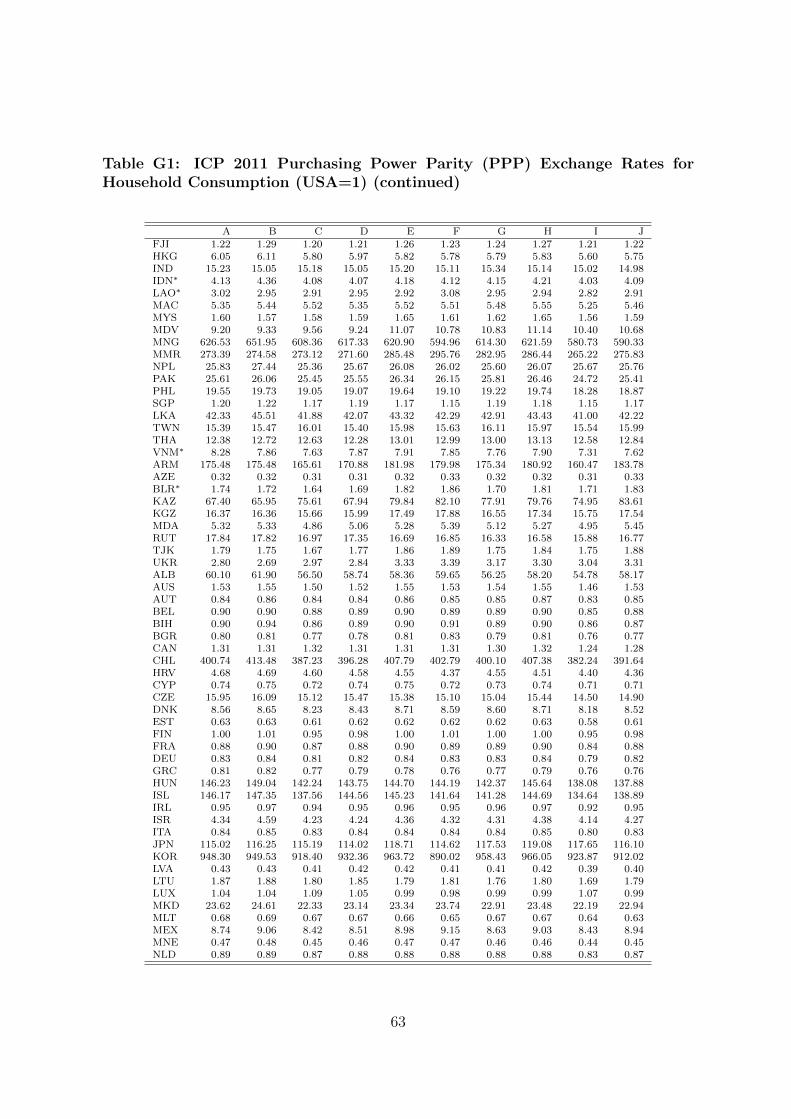
Table G1: ICP 2011 Purchasing Power Parity (PPP) Exchange Rates forHousehold Consumption (USA=1) (continued)
A B C D E F G H I JFJI 1.22 1.29 1.20 1.21 1.26 1.23 1.24 1.27 1.21 1.22HKG 6.05 6.11 5.80 5.97 5.82 5.78 5.79 5.83 5.60 5.75IND 15.23 15.05 15.18 15.05 15.20 15.11 15.34 15.14 15.02 14.98IDN∗ 4.13 4.36 4.08 4.07 4.18 4.12 4.15 4.21 4.03 4.09LAO∗ 3.02 2.95 2.91 2.95 2.92 3.08 2.95 2.94 2.82 2.91MAC 5.35 5.44 5.52 5.35 5.52 5.51 5.48 5.55 5.25 5.46MYS 1.60 1.57 1.58 1.59 1.65 1.61 1.62 1.65 1.56 1.59MDV 9.20 9.33 9.56 9.24 11.07 10.78 10.83 11.14 10.40 10.68MNG 626.53 651.95 608.36 617.33 620.90 594.96 614.30 621.59 580.73 590.33MMR 273.39 274.58 273.12 271.60 285.48 295.76 282.95 286.44 265.22 275.83NPL 25.83 27.44 25.36 25.67 26.08 26.02 25.60 26.07 25.67 25.76PAK 25.61 26.06 25.45 25.55 26.34 26.15 25.81 26.46 24.72 25.41PHL 19.55 19.73 19.05 19.07 19.64 19.10 19.22 19.74 18.28 18.87SGP 1.20 1.22 1.17 1.19 1.17 1.15 1.19 1.18 1.15 1.17LKA 42.33 45.51 41.88 42.07 43.32 42.29 42.91 43.43 41.00 42.22TWN 15.39 15.47 16.01 15.40 15.98 15.63 16.11 15.97 15.54 15.99THA 12.38 12.72 12.63 12.28 13.01 12.99 13.00 13.13 12.58 12.84VNM∗ 8.28 7.86 7.63 7.87 7.91 7.85 7.76 7.90 7.31 7.62ARM 175.48 175.48 165.61 170.88 181.98 179.98 175.34 180.92 160.47 183.78AZE 0.32 0.32 0.31 0.31 0.32 0.33 0.32 0.32 0.31 0.33BLR∗ 1.74 1.72 1.64 1.69 1.82 1.86 1.70 1.81 1.71 1.83KAZ 67.40 65.95 75.61 67.94 79.84 82.10 77.91 79.76 74.95 83.61KGZ 16.37 16.36 15.66 15.99 17.49 17.88 16.55 17.34 15.75 17.54MDA 5.32 5.33 4.86 5.06 5.28 5.39 5.12 5.27 4.95 5.45RUT 17.84 17.82 16.97 17.35 16.69 16.85 16.33 16.58 15.88 16.77TJK 1.79 1.75 1.67 1.77 1.86 1.89 1.75 1.84 1.75 1.88UKR 2.80 2.69 2.97 2.84 3.33 3.39 3.17 3.30 3.04 3.31ALB 60.10 61.90 56.50 58.74 58.36 59.65 56.25 58.20 54.78 58.17AUS 1.53 1.55 1.50 1.52 1.55 1.53 1.54 1.55 1.46 1.53AUT 0.84 0.86 0.84 0.84 0.86 0.85 0.85 0.87 0.83 0.85BEL 0.90 0.90 0.88 0.89 0.90 0.89 0.89 0.90 0.85 0.88BIH 0.90 0.94 0.86 0.89 0.90 0.91 0.89 0.90 0.86 0.87BGR 0.80 0.81 0.77 0.78 0.81 0.83 0.79 0.81 0.76 0.77CAN 1.31 1.31 1.32 1.31 1.31 1.31 1.30 1.32 1.24 1.28CHL 400.74 413.48 387.23 396.28 407.79 402.79 400.10 407.38 382.24 391.64HRV 4.68 4.69 4.60 4.58 4.55 4.37 4.55 4.51 4.40 4.36CYP 0.74 0.75 0.72 0.74 0.75 0.72 0.73 0.74 0.71 0.71CZE 15.95 16.09 15.12 15.47 15.38 15.10 15.04 15.44 14.50 14.90DNK 8.56 8.65 8.23 8.43 8.71 8.59 8.60 8.71 8.18 8.52EST 0.63 0.63 0.61 0.62 0.62 0.62 0.62 0.63 0.58 0.61FIN 1.00 1.01 0.95 0.98 1.00 1.01 1.00 1.00 0.95 0.98FRA 0.88 0.90 0.87 0.88 0.90 0.89 0.89 0.90 0.84 0.88DEU 0.83 0.84 0.81 0.82 0.84 0.83 0.83 0.84 0.79 0.82GRC 0.81 0.82 0.77 0.79 0.78 0.76 0.77 0.79 0.76 0.76HUN 146.23 149.04 142.24 143.75 144.70 144.19 142.37 145.64 138.08 137.88ISL 146.17 147.35 137.56 144.56 145.23 141.64 141.28 144.69 134.64 138.89IRL 0.95 0.97 0.94 0.95 0.96 0.95 0.96 0.97 0.92 0.95ISR 4.34 4.59 4.23 4.24 4.36 4.32 4.31 4.38 4.14 4.27ITA 0.84 0.85 0.83 0.84 0.84 0.84 0.84 0.85 0.80 0.83JPN 115.02 116.25 115.19 114.02 118.71 114.62 117.53 119.08 117.65 116.10KOR 948.30 949.53 918.40 932.36 963.72 890.02 958.43 966.05 923.87 912.02LVA 0.43 0.43 0.41 0.42 0.42 0.41 0.41 0.42 0.39 0.40LTU 1.87 1.88 1.80 1.85 1.79 1.81 1.76 1.80 1.69 1.79LUX 1.04 1.04 1.09 1.05 0.99 0.98 0.99 0.99 1.07 0.99MKD 23.62 24.61 22.33 23.14 23.34 23.74 22.91 23.48 22.19 22.94MLT 0.68 0.69 0.67 0.67 0.66 0.65 0.67 0.67 0.64 0.63MEX 8.74 9.06 8.42 8.51 8.98 9.15 8.63 9.03 8.43 8.94MNE 0.47 0.48 0.45 0.46 0.47 0.47 0.46 0.46 0.44 0.45NLD 0.89 0.89 0.87 0.88 0.88 0.88 0.88 0.88 0.83 0.87
63

Table G1: ICP 2011 Purchasing Power Parity (PPP) Exchange Rates forHousehold Consumption (USA=1) (continued)
A B C D E F G H I JNZL 1.57 1.57 1.57 1.57 1.63 1.59 1.61 1.62 1.52 1.59NOR 10.13 10.18 9.68 9.82 10.21 10.02 10.01 10.17 9.32 9.80POL 2.01 2.04 1.91 1.97 1.97 1.94 1.92 1.97 1.85 1.94PRT 0.72 0.71 0.68 0.70 0.72 0.70 0.71 0.72 0.67 0.70ROU 2.11 2.15 1.99 2.07 2.09 2.12 2.03 2.09 1.95 2.00SRB 47.10 47.92 44.88 46.38 47.08 46.81 46.51 47.42 44.54 45.37SVK 0.60 0.61 0.57 0.59 0.59 0.58 0.58 0.59 0.55 0.57SVN 0.70 0.69 0.70 0.70 0.70 0.69 0.69 0.70 0.67 0.68ESP 0.78 0.79 0.76 0.77 0.79 0.77 0.78 0.79 0.76 0.78SWE 9.35 9.40 8.88 9.10 9.31 9.25 9.17 9.32 8.82 9.11CHE 1.58 1.60 1.54 1.55 1.59 1.59 1.58 1.59 1.55 1.61TUR 1.23 1.26 1.17 1.20 1.21 1.23 1.20 1.21 1.15 1.16GBR 0.77 0.78 0.76 0.77 0.77 0.78 0.77 0.77 0.73 0.76USA 1.00 1.00 1.00 1.00 1.00 1.00 1.00 1.00 1.00 1.00BOL 2.75 3.34 2.86 2.71 3.04 2.95 2.97 3.05 2.83 2.91BRA 1.65 1.71 1.58 1.61 1.74 1.73 1.70 1.74 1.63 1.66COL∗ 1.17 1.16 1.19 1.17 1.22 1.22 1.21 1.23 1.15 1.20CRI 356.68 380.01 347.10 352.21 361.42 356.01 354.97 362.32 345.84 343.79DOM 21.43 22.91 20.53 20.75 21.37 20.81 20.94 21.38 20.03 20.74ECU 0.57 0.61 0.54 0.56 0.56 0.54 0.56 0.57 0.54 0.55SLV 0.56 0.59 0.53 0.54 0.55 0.54 0.55 0.55 0.52 0.53GTM 4.07 4.08 3.93 3.99 4.13 3.95 4.05 4.12 3.92 3.87HTI 22.11 22.73 20.92 21.69 21.55 21.83 21.13 21.62 20.82 20.71HND 10.24 11.14 10.03 9.99 10.50 10.25 10.26 10.50 9.95 10.08NIC 9.44 10.27 9.17 9.20 9.67 9.21 9.59 9.66 8.91 9.16PAN 0.58 0.62 0.55 0.56 0.57 0.56 0.56 0.57 0.54 0.55PRY∗ 2.42 2.59 2.30 2.36 2.40 2.40 2.33 2.38 2.27 2.31PER 1.56 1.63 1.57 1.54 1.63 1.60 1.61 1.64 1.54 1.57URY 16.51 17.81 16.40 16.19 17.06 16.71 16.89 17.13 16.06 16.42VEN 3.32 3.02 3.11 3.28 3.35 3.35 3.36 3.37 2.97 2.92BHR 0.23 0.25 0.23 0.23 0.22 0.23 0.23 0.23 0.21 0.22IRQ 592.91 593.93 570.13 580.02 608.97 617.19 591.90 606.03 570.58 573.42JOR 0.32 0.32 0.32 0.32 0.34 0.34 0.33 0.34 0.32 0.32KWT 0.19 0.21 0.19 0.19 0.19 0.19 0.20 0.19 0.18 0.18OMN 0.22 0.24 0.21 0.21 0.21 0.22 0.21 0.21 0.20 0.20PSE 2.43 2.45 2.35 2.40 2.49 2.50 2.44 2.49 2.37 2.52QAT 2.88 3.12 2.83 2.85 2.85 2.81 2.90 2.88 2.82 2.64SAU 1.84 1.99 1.83 1.81 1.87 1.86 1.87 1.88 1.77 1.79ARE 2.68 3.01 2.82 2.68 2.86 2.86 2.85 2.86 2.71 2.72YEM 78.96 79.79 79.51 78.22 85.81 85.23 85.05 85.79 79.42 82.09IRN∗ 4.79 4.84 4.78 4.74 5.03 5.01 4.98 5.00 4.70 5.00GEO 0.80 0.80 0.76 0.78 0.81 0.82 0.79 0.81 0.71 0.84
Notes: (i) The PPP methods are as follows: A = MST(LPS); B = SP-GEKS(LPS); C = SP-Union(LPS);
D = SP-Sum(LPS); E = MST(W1); F = SP-GEKS(W1); G = SP-Union(W1); H = SP-Sum(W1); I =
GEKS; J = Official ICP 2011 Results.
(ii) The country codes are shown in Table G2.
(iii) ∗ The PPP has been divided by 1 000.
64
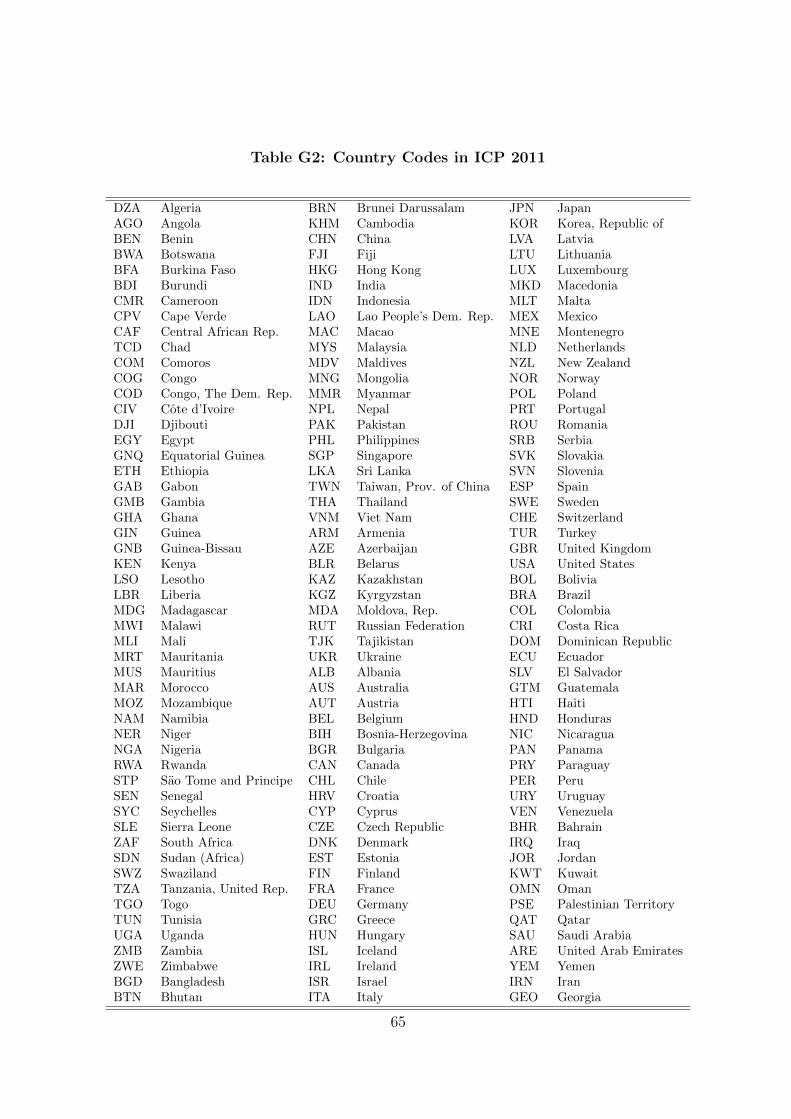
Table G2: Country Codes in ICP 2011
DZA Algeria BRN Brunei Darussalam JPN JapanAGO Angola KHM Cambodia KOR Korea, Republic ofBEN Benin CHN China LVA LatviaBWA Botswana FJI Fiji LTU LithuaniaBFA Burkina Faso HKG Hong Kong LUX LuxembourgBDI Burundi IND India MKD MacedoniaCMR Cameroon IDN Indonesia MLT MaltaCPV Cape Verde LAO Lao People’s Dem. Rep. MEX MexicoCAF Central African Rep. MAC Macao MNE MontenegroTCD Chad MYS Malaysia NLD NetherlandsCOM Comoros MDV Maldives NZL New ZealandCOG Congo MNG Mongolia NOR NorwayCOD Congo, The Dem. Rep. MMR Myanmar POL PolandCIV Cote d’Ivoire NPL Nepal PRT PortugalDJI Djibouti PAK Pakistan ROU RomaniaEGY Egypt PHL Philippines SRB SerbiaGNQ Equatorial Guinea SGP Singapore SVK SlovakiaETH Ethiopia LKA Sri Lanka SVN SloveniaGAB Gabon TWN Taiwan, Prov. of China ESP SpainGMB Gambia THA Thailand SWE SwedenGHA Ghana VNM Viet Nam CHE SwitzerlandGIN Guinea ARM Armenia TUR TurkeyGNB Guinea-Bissau AZE Azerbaijan GBR United KingdomKEN Kenya BLR Belarus USA United StatesLSO Lesotho KAZ Kazakhstan BOL BoliviaLBR Liberia KGZ Kyrgyzstan BRA BrazilMDG Madagascar MDA Moldova, Rep. COL ColombiaMWI Malawi RUT Russian Federation CRI Costa RicaMLI Mali TJK Tajikistan DOM Dominican RepublicMRT Mauritania UKR Ukraine ECU EcuadorMUS Mauritius ALB Albania SLV El SalvadorMAR Morocco AUS Australia GTM GuatemalaMOZ Mozambique AUT Austria HTI HaitiNAM Namibia BEL Belgium HND HondurasNER Niger BIH Bosnia-Herzegovina NIC NicaraguaNGA Nigeria BGR Bulgaria PAN PanamaRWA Rwanda CAN Canada PRY ParaguaySTP Sao Tome and Principe CHL Chile PER PeruSEN Senegal HRV Croatia URY UruguaySYC Seychelles CYP Cyprus VEN VenezuelaSLE Sierra Leone CZE Czech Republic BHR BahrainZAF South Africa DNK Denmark IRQ IraqSDN Sudan (Africa) EST Estonia JOR JordanSWZ Swaziland FIN Finland KWT KuwaitTZA Tanzania, United Rep. FRA France OMN OmanTGO Togo DEU Germany PSE Palestinian TerritoryTUN Tunisia GRC Greece QAT QatarUGA Uganda HUN Hungary SAU Saudi ArabiaZMB Zambia ISL Iceland ARE United Arab EmiratesZWE Zimbabwe IRL Ireland YEM YemenBGD Bangladesh ISR Israel IRN IranBTN Bhutan ITA Italy GEO Georgia
65

Table G3: ICP 2011 Real Per Capita Household Income (Based on PPP-Exchange Rates for Household Consumption) in US Dollars
A B D D E F G H I JDZA 3870 3818 3724 3853 3725 3410 3834 3667 3979 3983AGO 3193 2892 3309 3242 3309 3601 3302 3289 3387 3423BEN 1173 1117 1239 1195 1218 1240 1243 1217 1266 1286BWA 5111 4703 5154 5135 5054 5386 5112 5033 5359 5396BFA 763 812 815 776 794 824 807 797 812 840BDI 425 437 473 434 490 469 519 491 529 537CMR 1870 1783 1940 1859 1885 1899 1957 1888 2022 2063CPV 3778 3678 3777 3833 3650 3828 3747 3638 3917 3907CAF 703 638 746 714 719 729 751 734 762 770TCD 1226 1134 1271 1239 1230 1259 1280 1240 1322 1316COM 525 481 539 525 527 551 536 530 579 563COG 1163 1225 1240 1218 1185 1185 1220 1191 1292 1265COD 378 388 382 380 369 369 378 368 398 393CIV 1519 1448 1623 1552 1647 1698 1691 1635 1753 1746DJI 1354 1148 1375 1353 1432 1522 1444 1426 1509 1482EGY 7913 7952 7403 8071 7355 7371 7091 7303 7469 7218GNQ 4018 4184 4268 4189 4092 4063 4204 4104 4556 4340ETH 866 628 849 859 821 839 836 824 878 863GAB 5215 4918 5164 5214 4828 4787 4975 4836 5213 5104GMB 1066 959 1010 1060 1002 999 1014 995 1101 1051GHA 1906 1765 1853 1901 1752 1735 1822 1753 1954 1868GIN 688 583 697 687 645 624 681 655 730 701GNB 778 695 776 780 767 776 786 764 824 810KEN 1521 1503 1531 1524 1513 1575 1516 1494 1570 1563LSO 2011 2029 2013 1995 1987 2138 2018 1977 2097 2098LBR 475 427 522 483 529 530 537 527 584 551MDG 1096 993 1166 1130 1137 1143 1148 1132 1158 1187MWI 842 713 857 844 833 888 855 830 903 885MLI 854 857 863 844 834 874 868 835 896 905MRT 1537 1490 1589 1559 1581 1664 1631 1588 1670 1699MUS 8882 8602 9291 9007 9388 10469 9440 9391 9889 9927MAR 3366 3528 3428 3427 3365 3625 3382 3343 3539 3495MOZ 748 812 763 756 733 739 755 730 771 782NAM 4665 4602 4651 4684 4459 4449 4582 4452 4843 4689NER 581 551 616 592 590 608 613 594 638 637NGA 1685 1580 1709 1710 1677 1646 1730 1677 1831 1768RWA 924 950 1029 944 1098 1020 1099 1089 1164 1178STP 2592 2544 2758 2719 2695 2714 2771 2691 2860 2864SEN 1560 1497 1640 1598 1588 1673 1635 1597 1693 1691SYC 9600 9303 10198 9740 9728 10163 9799 9735 10098 10102SLE 1085 963 1031 1096 986 1004 1016 987 1119 1053ZAF 6670 6807 6751 6645 6495 6789 6530 6455 6767 6772SDN 2047 2037 2085 2075 1996 2045 2056 1998 2122 2069SWZ 4854 4864 4979 4907 4913 5099 4960 4925 5148 5152TZA 828 817 852 834 871 904 883 867 905 917TGO 912 815 993 936 953 992 986 960 1050 1031TUN 5716 5713 5792 5846 5667 5846 5699 5674 5906 5758UGA 1046 929 1098 1052 1092 1109 1106 1074 1160 1156ZMB 1442 1194 1480 1446 1457 1557 1497 1453 1535 1555ZWE 977 914 1043 1024 1043 1100 1078 1051 1101 1134BGD 1916 1781 1947 1927 1998 1927 1952 1994 2018 1923BTN 3236 3248 3173 3199 3068 3107 3117 3072 3212 3127BRN 11846 12483 12008 11906 11787 12152 11616 11804 12041 12190KHM 1945 1929 1916 1959 1820 1881 1874 1834 1966 1907CHN 3388 3435 3304 3372 3214 3285 3245 3210 3363 3277FJI 4579 4344 4686 4649 4441 4559 4538 4414 4632 4611HKG 28643 28341 29847 29001 29749 29986 29913 29696 30914 30104
66

Table G3: ICP 2011 Real Per Capita Household Income (Based on PPP-Exchange Rates for Household Consumption) in US Dollars (continued)
A B C D E F G H I JIND 2626 2657 2635 2659 2631 2648 2609 2642 2664 2672IDN 4071 3857 4122 4128 4023 4086 4054 3994 4175 4110LAO 1905 1951 1980 1954 1968 1869 1952 1956 2040 1975MAC 20297 19977 19693 20317 19676 19717 19825 19574 20679 19887MYS 9027 9201 9134 9103 8753 8956 8899 8760 9256 9105MDV 3403 3358 3275 3388 2830 2905 2892 2812 3012 2934MNG 4102 3942 4225 4163 4139 4320 4184 4135 4425 4354MMR 1742 1735 1744 1754 1668 1610 1683 1663 1796 1727NPL 1629 1533 1659 1639 1613 1617 1644 1614 1639 1633PAK 3464 3404 3486 3473 3368 3392 3437 3353 3588 3491PHL 3875 3839 3975 3971 3855 3965 3940 3837 4144 4013SGP 20856 20663 21461 21100 21434 21863 21151 21191 21904 21444LKA 5171 4810 5227 5203 5053 5176 5101 5040 5339 5185TWN 23047 22921 22147 23020 22191 22687 22015 22208 22811 22169THA 7259 7068 7118 7321 6911 6920 6914 6847 7146 6998VNM 2252 2373 2443 2371 2359 2376 2404 2362 2550 2446ARM 5973 5973 6329 6134 5760 5824 5978 5794 6532 5704AZE 6649 6647 6964 6806 6605 6481 6634 6620 6902 6507BLR 8577 8716 9124 8847 8197 8046 8770 8268 8720 8160KAZ 10566 10800 9419 10482 8921 8674 9141 8929 9503 8518KGZ 2770 2772 2896 2836 2593 2537 2741 2615 2880 2586MDA 4198 4189 4598 4416 4231 4144 4358 4237 4509 4097RUT 10742 10756 11292 11048 11483 11374 11735 11556 12071 11429TJK 2334 2384 2490 2362 2246 2202 2389 2263 2379 2215UKR 6853 7116 6447 6749 5757 5659 6048 5806 6307 5785ALB 6049 5874 6436 6190 6230 6096 6463 6248 6638 6251AUS 22208 21913 22694 22360 22013 22246 22143 21944 23226 22288AUT 23249 22845 23212 23344 22609 23049 22876 22585 23455 23049BEL 19728 19610 20190 19835 19651 19908 19831 19652 20985 20173BIH 6406 6148 6691 6526 6397 6373 6526 6402 6747 6667BGR 8030 7934 8257 8192 7874 7665 8047 7854 8383 8358CAN 21662 21664 21611 21665 21694 21664 21781 21598 22904 22127CHL 10752 10421 11127 10873 10566 10697 10769 10577 11272 11002HRV 9877 9871 10059 10100 10164 10580 10179 10257 10518 10616CYP 19287 19077 19792 19359 18869 19666 19488 19109 20089 19999CZE 11562 11461 12191 11916 11991 12209 12258 11943 12717 12372DNK 18304 18103 19032 18584 17982 18244 18216 17994 19157 18379EST 9785 9708 9989 9902 9844 9875 9896 9762 10460 10051FIN 19619 19407 20650 19997 19530 19408 19545 19504 20567 19917FRA 20064 19740 20331 20119 19679 19966 19896 19702 20999 20167DEU 22197 21915 22571 22416 21848 22111 22086 21852 23247 22398GRC 17095 16782 17978 17345 17556 18014 17812 17536 18029 18156HUN 10099 9909 10383 10273 10206 10242 10372 10140 10695 10710ISL 18117 17972 19251 18319 18234 18697 18745 18303 19668 19066IRL 17918 17681 18223 18041 17816 17950 17793 17683 18612 17949ISR 15709 14842 16113 16083 15631 15791 15827 15564 16472 15963ITA 18881 18648 19189 19040 18908 18928 18984 18842 19922 19311JPN 19369 19164 19340 19538 18767 19436 18956 18708 18937 19188KOR 13884 13866 14336 14121 13662 14793 13737 13628 14251 14436LVA 10055 9984 10514 10260 10378 10402 10570 10318 11051 10700LTU 11863 11777 12303 11996 12359 12271 12593 12308 13088 12416LUX 24609 24598 23325 24210 25724 26089 25821 25732 23829 25804MKD 7100 6815 7512 7249 7185 7064 7320 7144 7558 7313MLT 14202 14072 14506 14569 14625 14952 14575 14530 15236 15455MEX 9536 9196 9901 9790 9283 9105 9662 9229 9888 9322MNE 9218 9011 9565 9265 9235 9225 9357 9254 9723 9565NLD 18354 18245 18784 18454 18464 18522 18509 18491 19536 18732
67

Table G3: ICP 2011 Real Per Capita Household Income (Based on PPP-Exchange Rates for Household Consumption) in US Dollars (continued)
A B C D E F G H I JNZL 17641 17641 17641 17641 17037 17413 17218 17051 18168 17425NOR 22550 22445 23608 23276 22384 22801 22820 22468 24515 23322POL 12051 11872 12667 12303 12335 12479 12608 12298 13074 12519PRT 14703 14915 15607 15273 14736 15157 15070 14751 15945 15112ROU 7855 7686 8303 7981 7921 7811 8152 7902 8474 8274SRB 7222 7099 7580 7335 7226 7267 7315 7174 7638 7498SVK 12241 11970 12888 12575 12528 12609 12740 12474 13300 12981SVN 14501 14570 14525 14475 14417 14705 14610 14365 15132 14856ESP 16972 16877 17587 17184 16713 17151 17013 16788 17513 17101SWE 18915 18814 19911 19429 18996 19112 19278 18977 20060 19424CHE 26945 26614 27766 27417 26770 26731 26994 26788 27469 26418TUR 10172 9913 10672 10445 10291 10148 10441 10316 10896 10729GBR 20485 20363 20923 20598 20450 20398 20444 20434 21767 20912USA 34329 34329 34329 34329 34329 34329 34329 34329 34329 34329BOL 3637 2991 3494 3687 3282 3383 3361 3269 3522 3436BRA 7897 7576 8218 8071 7476 7518 7639 7472 7971 7833COL 6919 6977 6825 6897 6620 6642 6714 6603 7055 6765CRI 8276 7768 8504 8381 8167 8292 8316 8147 8535 8586DOM 8528 7974 8901 8805 8551 8779 8724 8547 9124 8810ECU 5636 5266 5892 5742 5656 5957 5703 5630 5950 5832SLV 6198 5810 6504 6350 6260 6369 6244 6223 6579 6503GTM 5301 5289 5482 5399 5219 5463 5320 5226 5504 5565HTI 1509 1468 1595 1539 1548 1528 1579 1543 1603 1612HND 3269 3005 3338 3351 3188 3267 3262 3189 3364 3321NIC 3022 2777 3109 3099 2950 3096 2973 2953 3199 3113PAN 8721 8199 9218 8967 8832 8987 8934 8828 9311 9154PRY 4635 4344 4873 4753 4681 4679 4811 4709 4956 4862PER 6364 6090 6336 6431 6085 6218 6178 6065 6434 6332URY 10905 10109 10978 11122 10551 10775 10658 10513 11207 10962VEN 7652 8401 8152 7742 7577 7589 7551 7534 8561 8710BHR 15187 14040 15620 15441 15804 15605 15239 15532 17138 16419IRQ 3858 3851 4012 3944 3756 3706 3865 3774 4009 3989JOR 7320 7243 7372 7387 6960 6912 6987 6943 7371 7328KWT 17617 16288 17784 17892 17535 18124 17228 17505 19165 18653OMN 11381 10241 11513 11483 11608 11383 11752 11519 12357 12252PSE 3329 3309 3448 3374 3251 3233 3312 3250 3414 3209QAT 15694 14508 15975 15876 15857 16125 15620 15687 16043 17140SAU 13074 12089 13115 13280 12870 12890 12825 12797 13570 13457ARE 29913 26588 28405 29904 27970 27979 28076 27973 29510 29459YEM 2430 2405 2413 2453 2236 2251 2256 2237 2416 2337IRN 7106 7032 7113 7177 6770 6799 6829 6804 7245 6804GEO 5015 5015 5290 5137 4972 4890 5105 4979 5683 4789
Notes: (i) The PPP methods are again as follows: A = MST(LPS); B = SP-GEKS(LPS); C = SP-
Union(LPS); D = SP-Sum(LPS); E = MST(W1); F = SP-GEKS(W1); G = SP-Union(W1); H = SP-
Sum(W1); I = GEKS; J = Official ICP 2011 Results.
(ii) The country codes are shown in Table G2.
68

Additional Appendix References
Deaton A. (2012), “Calibrating Measurement Uncertainty in Purchasing Power Parity Ex-
change Rates,” Paper Presented to the World Bank’s ICP Technical Advisory Group.
Rao, D. S. P. and G. Hajargasht (2016), “Stochastic approach to computation of pur-
chasing power parities in the International Comparison Program (ICP),” Journal of
Econometrics 191(2), 414-425.
69

Graz Economics PapersFor full list see:
http://ideas.repec.org/s/grz/wpaper.html
Address: Department of Economics, University of Graz,
Universitatsstraße 15/F4, A-8010 Graz
04–2018 Robert J. Hill, Alicia N. Rambaldi, and Michael Scholz: Higher Frequency
Hedonic Property Price Indices: A State Space Approach
03–2018 Reza Hajargasht, Robert J. Hill, D. S. Prasada Rao, and Sriram Shankar:
Spatial Chaining in International Comparisons of Prices and Real Incomes
02–2018 Christoph Zwick: On the origin of current account deficits in the Euro area
periphery: A DSGE perspective
01–2018 Michael Greinecker and Christopher Kah: Pairwise stable matching in large
economies
15–2017 Florian Brugger and Jorn Kleinert: The strong increase of Austrian government
debt in the Kreisky era: Austro-Keynesianism or just stubborn forecast errors?
14–2017 Jakob Mayer, Gabriel Bachner and Karl W. Steininger: Macroeconomic
implications of switching to process-emission-free iron and steel production in Europe
13–2017 Andreas Darmann, Julia Grundner and Christian Klamler: Consensus in the
2015 Provincial Parliament Election in Styria, Austria: Voting Rules,Outcomes, and
the Condorcet Paradox
12–2017 Robert J. Hill, Miriam Steurer and Sofie R. Waltl: Owner Occupied Housing
in the CPI and Its Impact On Monetary Policy During Housing Booms and Busts
11–2017 Philipp Kohlgruber and Christoph Kuzmics: The distribution of article quality
and inefficiencies in the market for scientific journals

10–2017 Maximilian Goedl: The Sovereign-Bank Interaction in the Eurozone Crisis
09–2017 Florian Herold and Christoph Kuzmics: The evolution of taking roles
08–2017 Evangelos V. Dioikitopoulos, Stephen J. Turnovsky and Ronald Wendner:
Dynamic Status Effects, Savings, and Income Inequality
07–2017 Bo Chen, Yu Chen and David Rietzke: Simple Contracts under Observable and
Hidden Actions
06–2017 Stefan Borsky, Andrea Leiter and Michael Paffermayr: Product Quality and
Sustainability: The Effect of International Environmental Agreements on Bilateral
Trade
05–2017 Yadira Mori Clement and Birgit Bednar-Friedl: Do Clean Development
Mechanism projects generate local employment? Testing for sectoral effects across
Brazilian municipalities
04–2017 Stefan Borsky, Alexej Parchomenko: Identifying Phosphorus Hot Spots: A
spatial analysis of the phosphorus balance as a result of manure application
03–2017 Yu Chen, Yu Wang, Bonwoo Koo: Open Source and Competition Strategy
Under Network Effects
02–2017 Florian Brugger: The Effect of Foreign and Domestic Demand on U.S. Treasury
Yields
01–2017 Yu Chen: Simplifiability of Contingency Plans with Applications to Optimal
Mechanism Design
13–2016 Jan de Haan, Rens Hendriks, Michael Scholz: A Comparison of Weighted
Time-Product Dummy and Time Dummy Hedonic Indexes
12–2016 Katja Kalkschmied: Complementary Institutional Elements and Economic
Outcomes

11–2016 Dieter Balkenborg, Josef Hofbauer, Christoph Kuzmics: The refined best
reply correspondence and backward induction
10–2016 Karl W. Steininger, Wolf D. Grossmann, Iris Grossmann: The economic
value of dispatchable solar electricity: a Post-Paris evaluation
09–2016 Sofie R. Waltl: Estimating aggregate quantile-specific gross rental yields for
residential housing in Sydney
08–2016 Karl Farmer: Financial integration and house price dynamics in equilibrium
modeling of intra-EMU and global trade imbalances
07–2016 Gabriel Bachner, Birgit Bednar-Friedl: Counterbalancing the Effects of Climate
Change Adaptation on Public Budgets: Factor Taxes, Transfers, or Foreign Lending?
06–2016 Margareta Kreimer, Ricardo Mora: Segregated Integration: Recent Trends in
the Austrian Gender Division of Labor
05–2016 Karl Farmer, Bogdan Mihaiescu: Credit constraints and differential growth in
equilibrium modeling of EMU and global trade imbalances
04–2016 Daniel Eckert, Frederik Herzberg: The birth of social choice theory from the
spirit of mathematical logic: Arrow’s theorem in the framework of model theory
03–2016 Christoph Kuzmics, Jan-Henrik Steg: On public good provision mechanisms
with dominant strategies and balanced budget
02–2016 Florian Gauer, Christoph Kuzmics: Cognitive Empathy in Conflict Situations
01–2016 Thomas Aronsson, Olof Johansson-Stenman, Ronald Wendner:
Redistribution Through Charity, and Optimal Taxation when People are Concerned
with Social Status
09–2015 Sofie R. Waltl: Variation across price segments and locations: A comprehensive
quantile regression analysis of the Sydney housing market
08–2015 Karl Farmer, Bogdan Mihaiescu: Pension systems and financial constraints in a
three-country OLG model of intra-EMU and global trade imbalances
07–2015 Javier Lopez Prol, Karl W. Steininger: Photovoltaic self-consumption
regulation in Spain: profitability analysis and alternative regulation schemes.
06–2015 Miriam Steurer, Caroline Bayr: Quantifying Urban Sprawl using Land Use Data
05–2015 Porfirio Guevara, Robert J. Hill, Michael Scholz: Hedonic Indexes for Public
and Private Housing in Costa Rica
04–2015 Sofie R. Waltl: A Hedonic House Price Index in Continuous Time
03–2015 Ronald Wendner: Do Positional Preferences for Wealth and Consumption Cause
Inter-Temporal Distortions?
02–2015 Maximilian Godl, Christoph Zwick: Stochastic Stability of Public Debt: The
Case of Austria
01–2015 Gabriel Bachner: Land Transport Systems under Climate Change: A
Macroeconomic Assessment of Adaptation Measures for the Case of Austria