spatial interpolation - salisbury universityspatial interpolation inverse distance weighting the...

© Arthur J. Lembo, Jr.Salisbury University

Spatial InterpolationInverse Distance Weighting

The VariogramKriging

Much thanks to Bill Harper for his insights in Practical Geostatistics 2000 and personal conversation


Geostatistics• Includes a wide variety of techniques, including IDW,

nearest neighbor analysis and linear or nonlinear kriging, using one or more variables.

• Commonly used to identify and map spatial patterns across a landscape.

• Can be used to determine if spatial autocorrelation exists between data points. For this, the most common function used is the (semi)variogram. The variogram is a mathematical description of the relationship between the variance of pairs of observations (data points) and the distance separating these observations (h).

• Spatial autocorrelation can then be used to make better estimates for unsampled data points (inference = kriging).


Objectives• In this session we will evaluate a dataset and

attempt to:– Explore the theory and implementation of inverse

distance weighting– Evaluate issues with IDW interpolation– Explore the theory and implementation of the

semi-variogram and it’s applicability to interpolation

– Explore the theory and implementation of kriging and it’s applicability to interpolation


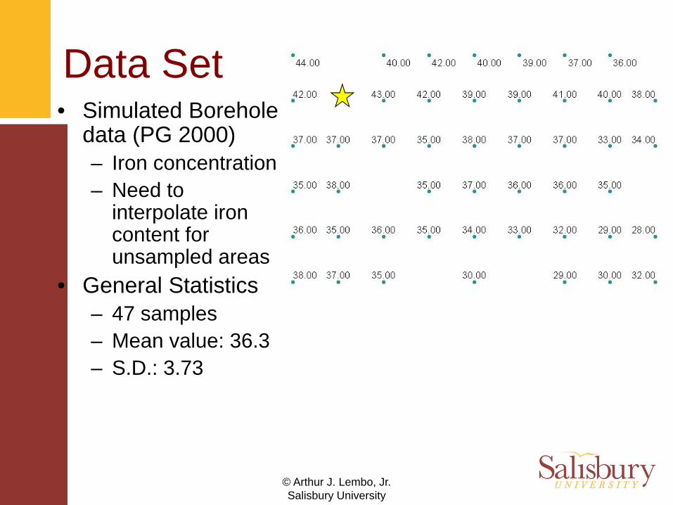
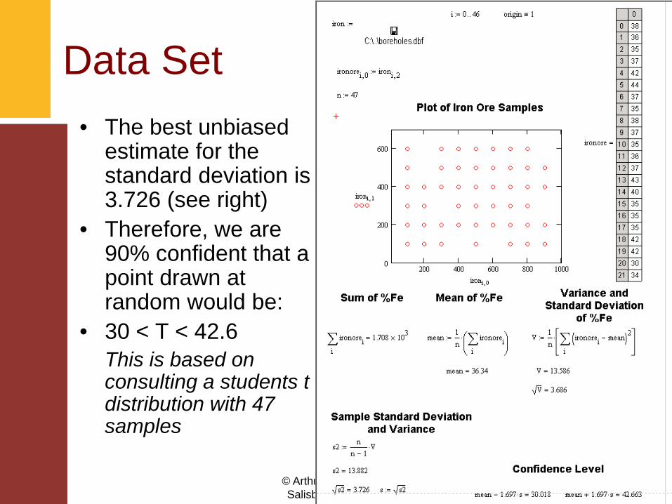
Data Set• Simulated Borehole

data (PG 2000)– Iron concentration– Need to

interpolate iron content for unsampled areas

• General Statistics– 47 samples– Mean value: 36.3– S.D.: 3.73


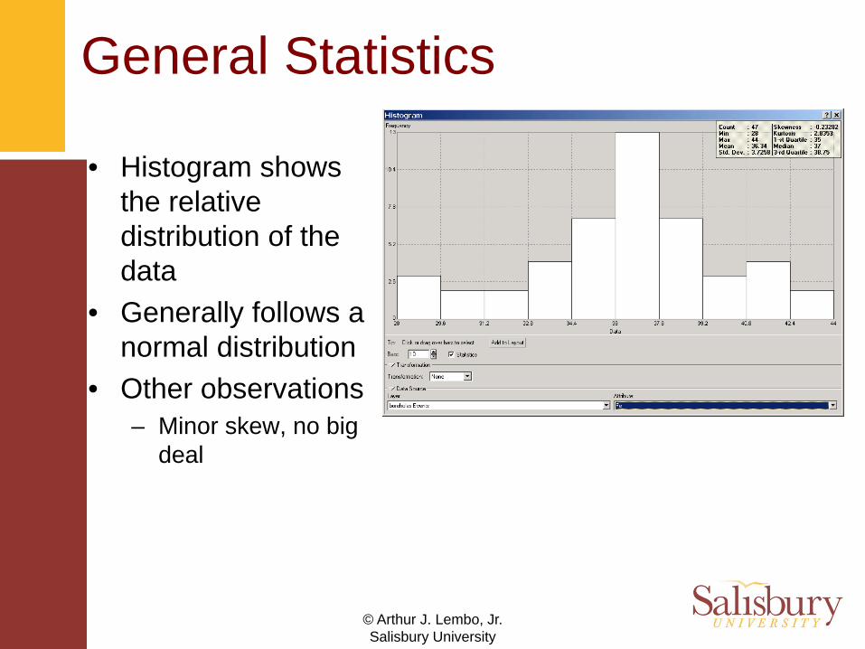
General Statistics

• Histogram shows the relative distribution of the data

• Generally follows a normal distribution

• Other observations– Minor skew, no big

deal


Data Set• The best unbiased

estimate for the standard deviation is 3.726 (see right)

• Therefore, we are 90% confident that a point drawn at random would be:

• 30 < T < 42.6This is based on consulting a students t distribution with 47 samples


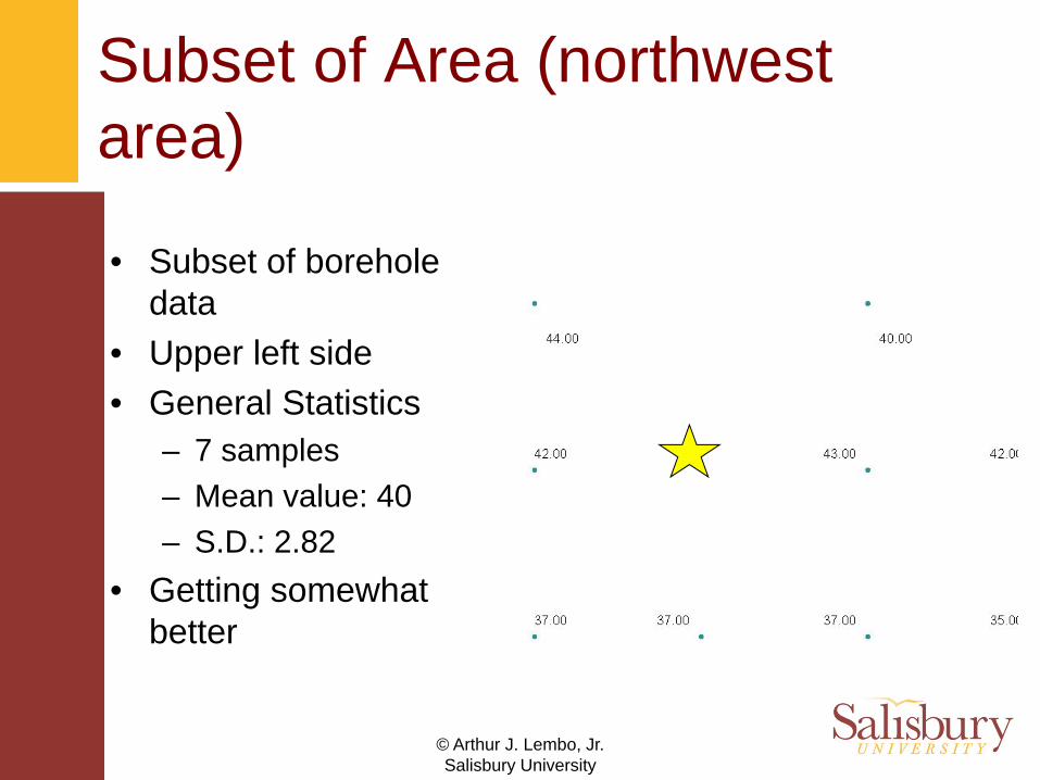
Subset of Area (northwest area)

• Subset of borehole data

• Upper left side• General Statistics

– 7 samples– Mean value: 40– S.D.: 2.82

• Getting somewhat better


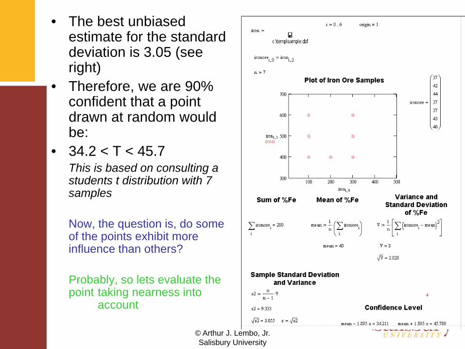
• The best unbiased estimate for the standard deviation is 3.05 (see right)


• 34.2 < T < 45.7This is based on consulting a students t distribution with 7 samples

Now, the question is, do some of the points exhibit more influence than others?

Probably, so lets evaluate the point taking nearness into

account


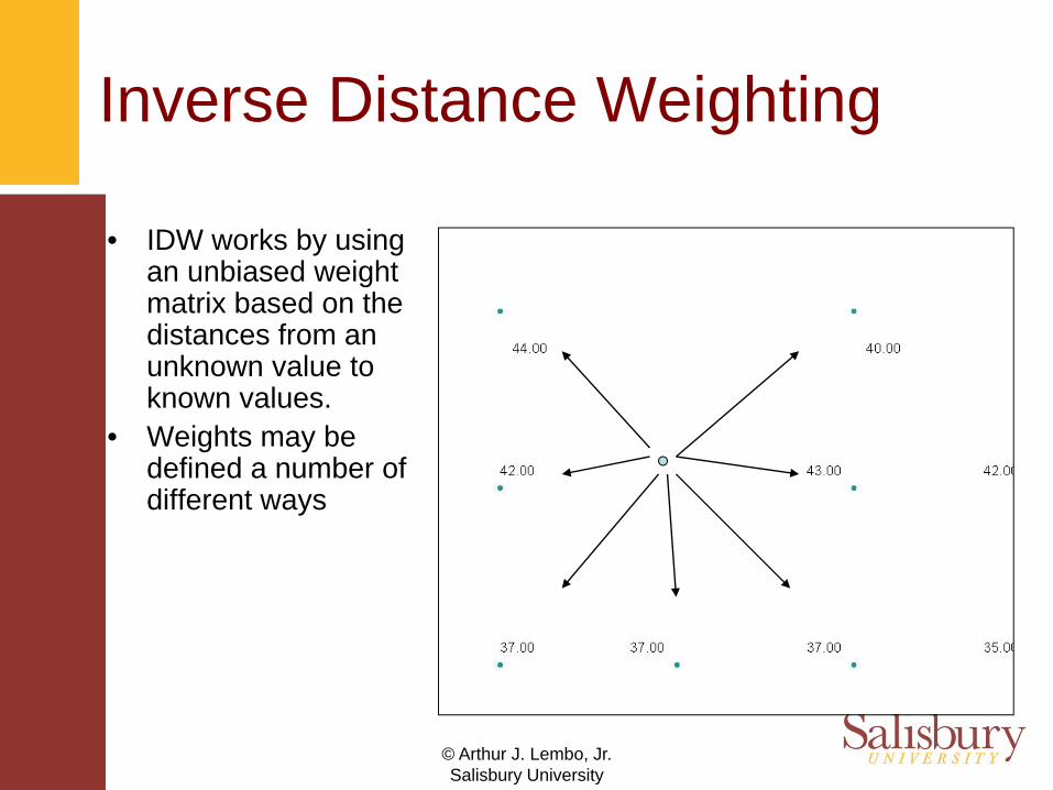
Inverse Distance Weighting

• IDW works by using an unbiased weight matrix based on the distances from an unknown value to known values.

• Weights may be defined a number of different ways


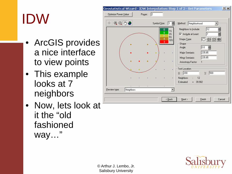
IDW• ArcGIS provides

a nice interface to view points

• This example looks at 7 neighbors

• Now, lets look at it the “old fashioned way…”


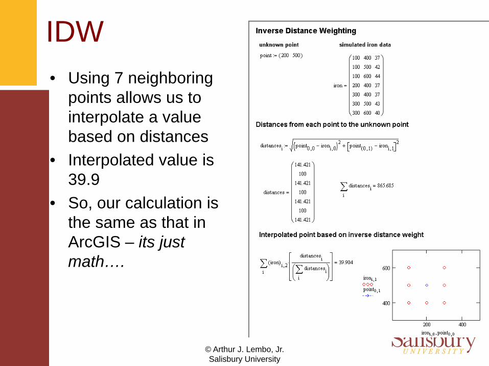
IDW• Using 7 neighboring

points allows us to interpolate a value based on distances

• Interpolated value is 39.9

• So, our calculation is the same as that in ArcGIS – its just math….


IDW –standard Error

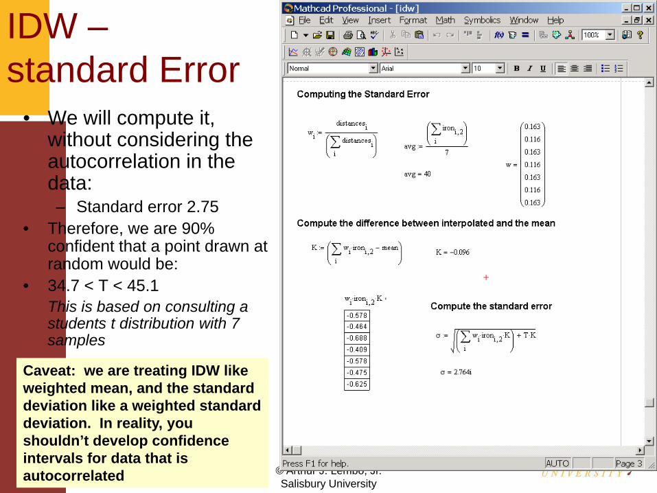
• We will compute it, without considering the autocorrelation in the data:– Standard error 2.75


• 34.7 < T < 45.1This is based on consulting a students t distribution with 7 samples

Caveat: we are treating IDW like weighted mean, and the standard deviation like a weighted standard deviation. In reality, you shouldn’t develop confidence intervals for data that is autocorrelated


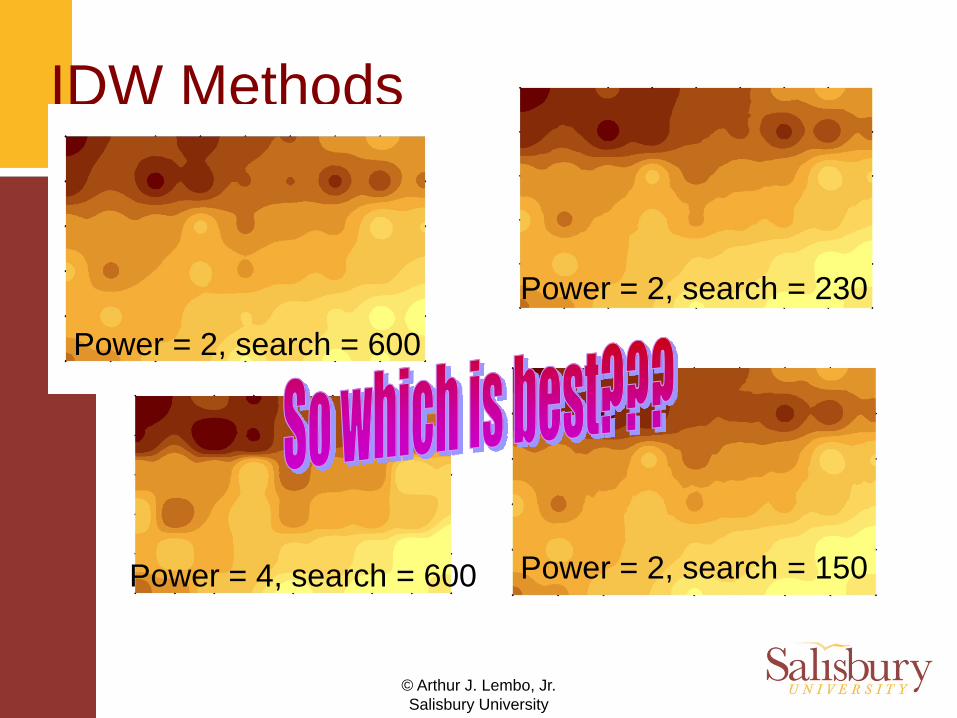
IDW Methods

Power = 2, search = 150





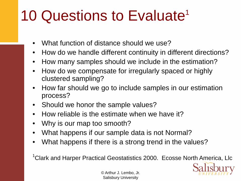
10 Questions to Evaluate1

• What function of distance should we use?• How do we handle different continuity in different directions?• How many samples should we include in the estimation?• How do we compensate for irregularly spaced or highly

clustered sampling?• How far should we go to include samples in our estimation

process?• Should we honor the sample values?• How reliable is the estimate when we have it?• Why is our map too smooth?• What happens if our sample data is not Normal?• What happens if there is a strong trend in the values?

1Clark and Harper Practical Geostatistics 2000. Ecosse North America, Llc


Answering the 10 Questions

The Variogram


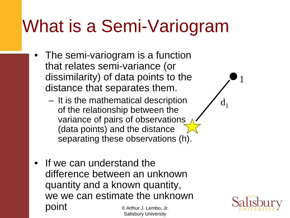
What is a Semi-Variogram• The semi-variogram is a function

that relates semi-variance (or dissimilarity) of data points to the distance that separates them. – It is the mathematical description

of the relationship between the variance of pairs of observations (data points) and the distance separating these observations (h).

• If we can understand the difference between an unknown quantity and a known quantity, we we can estimate the unknown point

1

d1


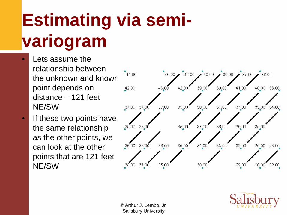
Estimating via semi-variogram• Lets assume the

relationship between the unknown and known point depends on distance – 121 feet NE/SW

• If these two points have the same relationship as the other points, we can look at the other points that are 121 feet NE/SW


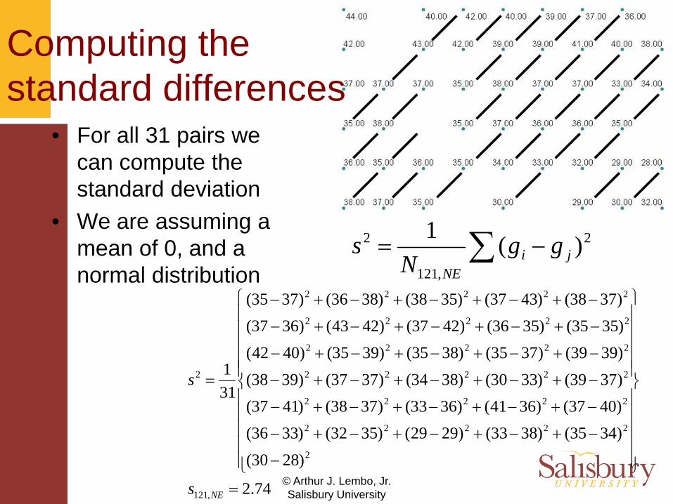
Computing the standard differences

• For all 31 pairs we can compute the standard deviation

• We are assuming a mean of 0, and a normal distribution

∑ −= 2

,121

2 )(1ji

NE

ggN

s

74.2

)2830()3435()3833()2929()3532()3336()4037()3641()3633()3738()4137()3739()3330()3834()3737()3938()3939()3735()3835()3935()4042()3535()3536()4237()4243()3637()3738()4337()3538()3836()3735(

311

,121

2

22222

22222

22222

22222

22222

22222

2

=

⎪⎪⎪⎪⎪

⎭

⎪⎪⎪⎪⎪

⎬

⎫

⎪⎪⎪⎪⎪

⎩

⎪⎪⎪⎪⎪

⎨

⎧

−

−+−+−+−+−

−+−+−+−+−

−+−+−+−+−

−+−+−+−+−

−+−+−+−+−

−+−+−+−+−

=

NEs

s


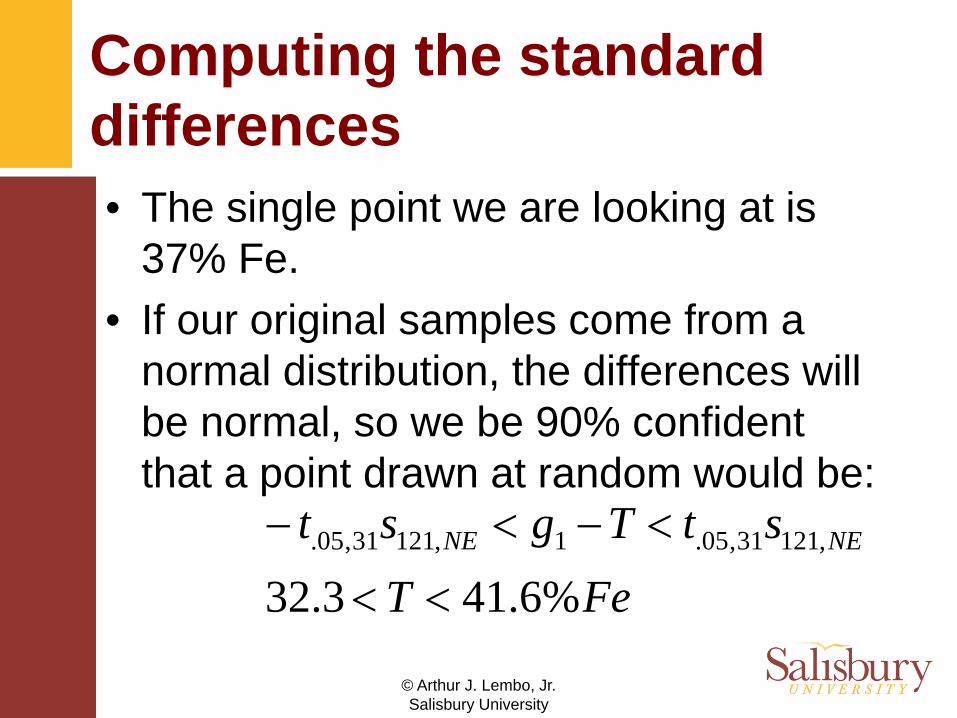
Computing the standard differences• The single point we are looking at is

37% Fe.• If our original samples come from a

normal distribution, the differences will be normal, so we be 90% confident that a point drawn at random would be:

FeTstTgst NENE

%6.413.32,12131,05.1,12131,05.

<<

<−<−


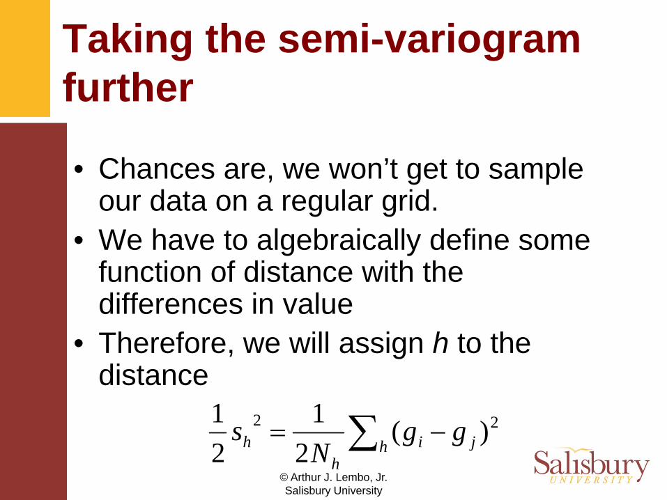
Taking the semi-variogram further

• Chances are, we won’t get to sample our data on a regular grid.

• We have to algebraically define some function of distance with the differences in value

• Therefore, we will assign h to the distance

∑ −=h ji

hh gg

Ns 22 )(

21

21


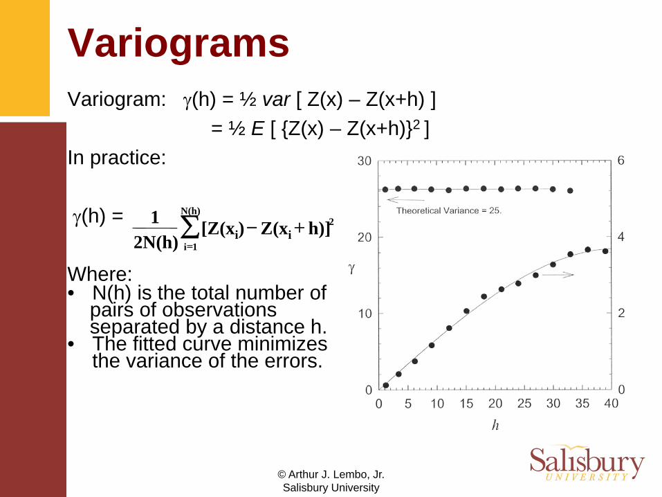
VariogramsVariogram: γ(h) = ½ var [ Z(x) – Z(x+h) ]

= ½ E [ {Z(x) – Z(x+h)}2 ]In practice:

γ(h) =

Where:• N(h) is the total number of

pairs of observations separated by a distance h.

• The fitted curve minimizes the variance of the errors.

∑=

+−N(h)

1i

2h)] Z(xi[Z(xi)2N(h)1


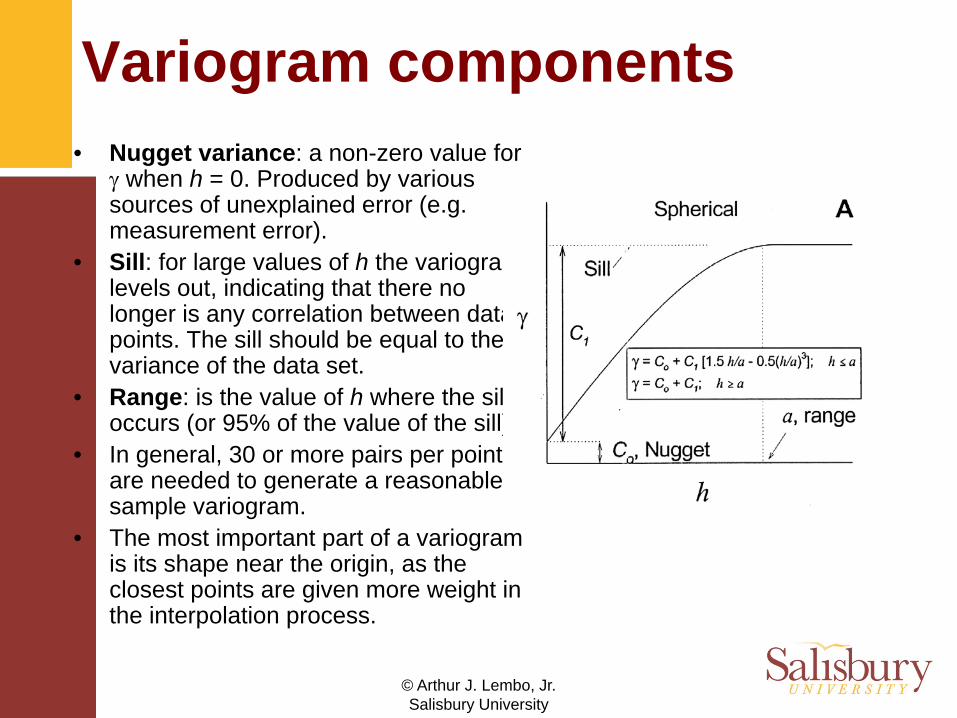
Variogram components• Nugget variance: a non-zero value for

γ when h = 0. Produced by various sources of unexplained error (e.g. measurement error).

• Sill: for large values of h the variogram levels out, indicating that there no longer is any correlation between data points. The sill should be equal to the variance of the data set.

• Range: is the value of h where the sill occurs (or 95% of the value of the sill).

• In general, 30 or more pairs per point are needed to generate a reasonable sample variogram.

• The most important part of a variogram is its shape near the origin, as the closest points are given more weight in the interpolation process.


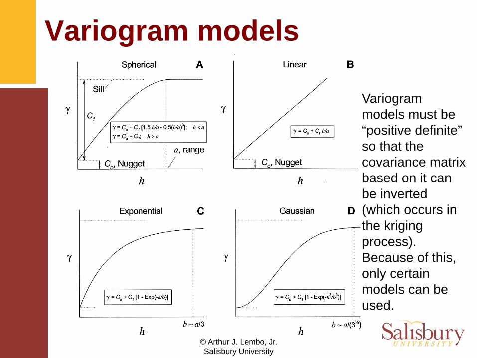
Variogram models

Variogram models must be “positive definite” so that the covariance matrix based on it can be inverted (which occurs in the kriging process). Because of this, only certain models can be used.


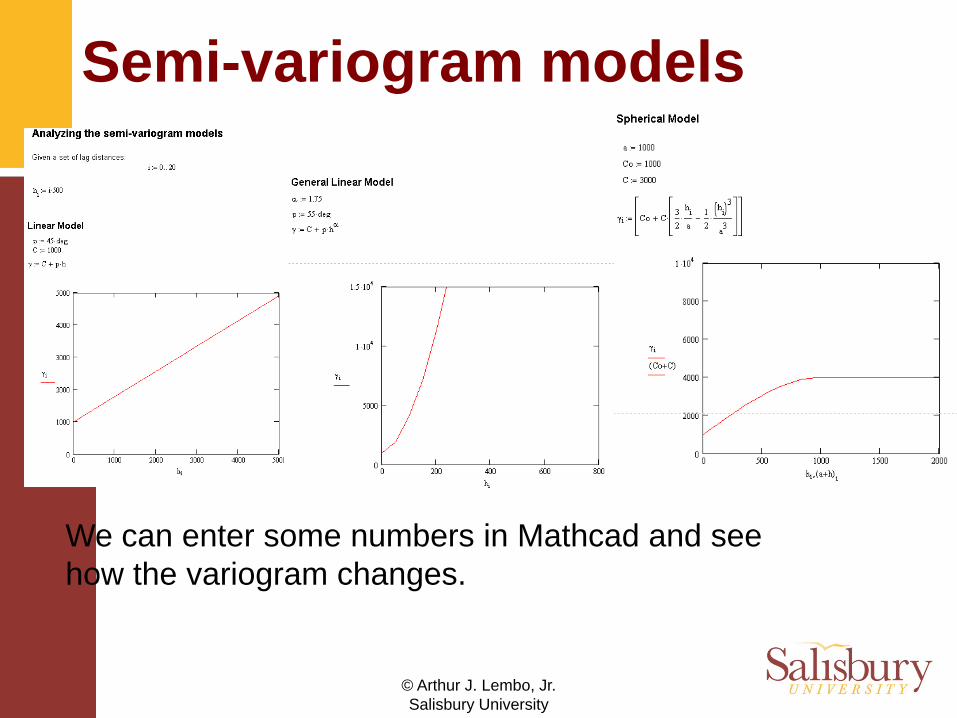
Semi-variogram models

We can enter some numbers in Mathcad and see how the variogram changes.


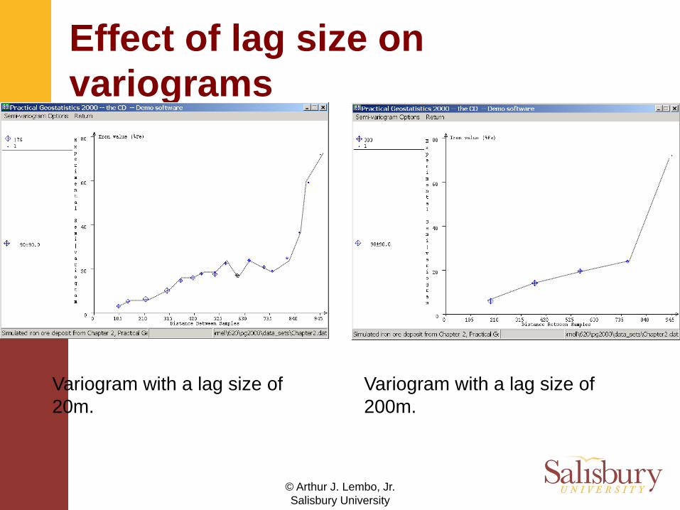
Effect of lag size on variograms

Variogram with a lag size of 20m.

Variogram with a lag size of 200m.


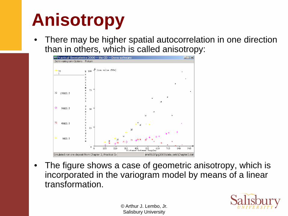
Anisotropy• There may be higher spatial autocorrelation in one direction

than in others, which is called anisotropy:

• The figure shows a case of geometric anisotropy, which is incorporated in the variogram model by means of a linear transformation.


Semi-variogram tips

• We are assuming a normal distribution• Gives us a picture of the relationship of

data values with distance.• If you don’t have a good spatial

structure in the semi-variogram, don’t revert to IDW – this is stupid!!!


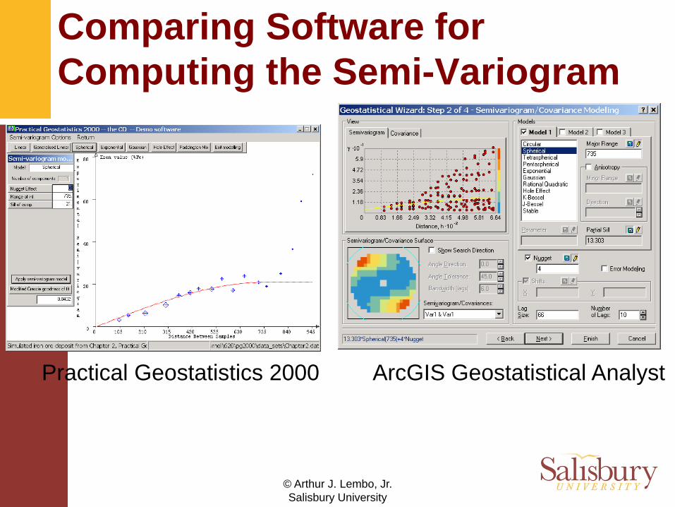
Comparing Software for Computing the Semi-Variogram

ArcGIS Geostatistical AnalystPractical Geostatistics 2000


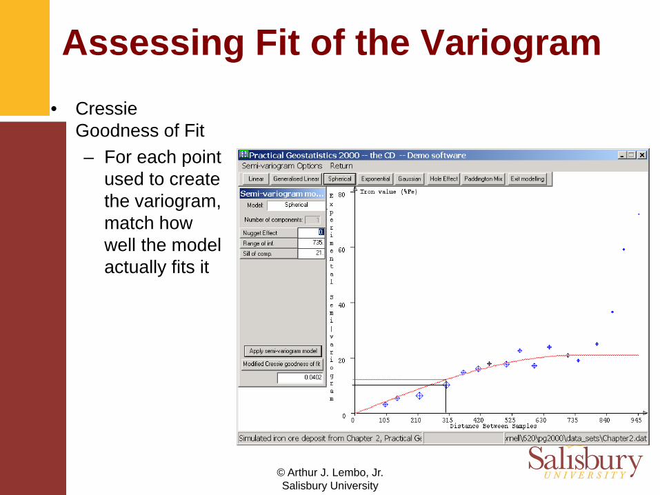
Assessing Fit of the Variogram• Cressie

Goodness of Fit– For each point

used to create the variogram, match how well the model actually fits it


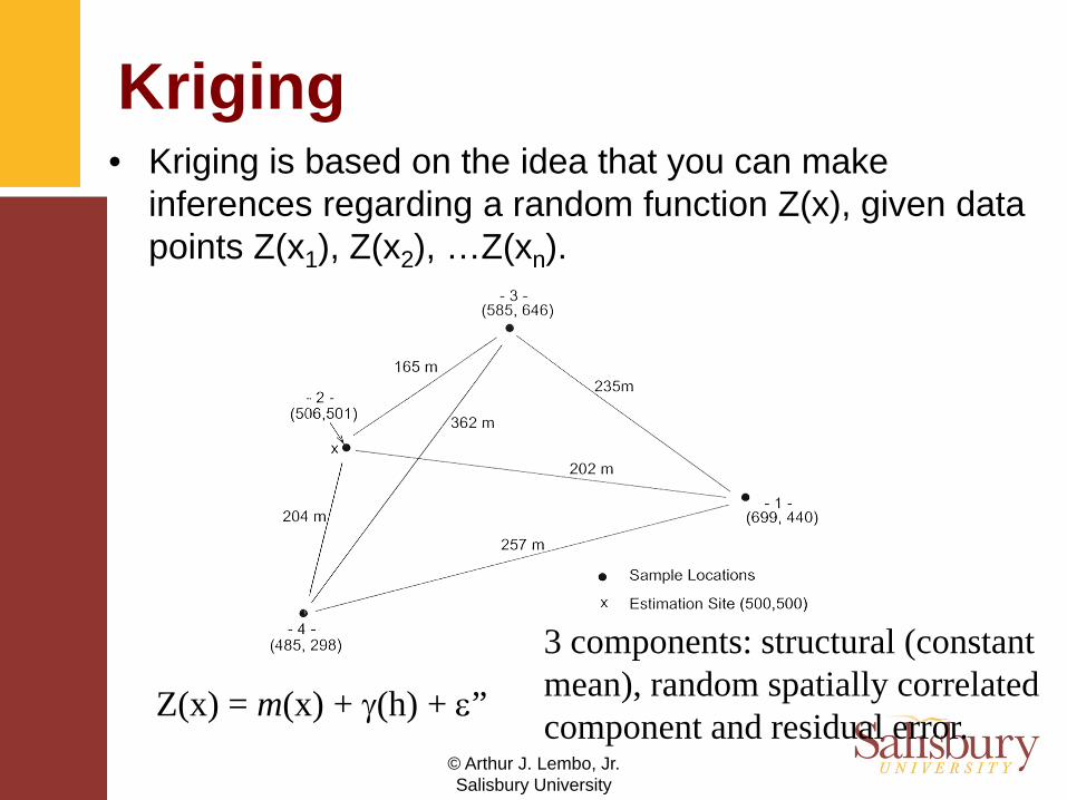
Kriging• Kriging is based on the idea that you can make

inferences regarding a random function Z(x), given data points Z(x1), Z(x2), …Z(xn).

Z(x) = m(x) + γ(h) + ε”

3 components: structural (constant mean), random spatially correlated component and residual error.


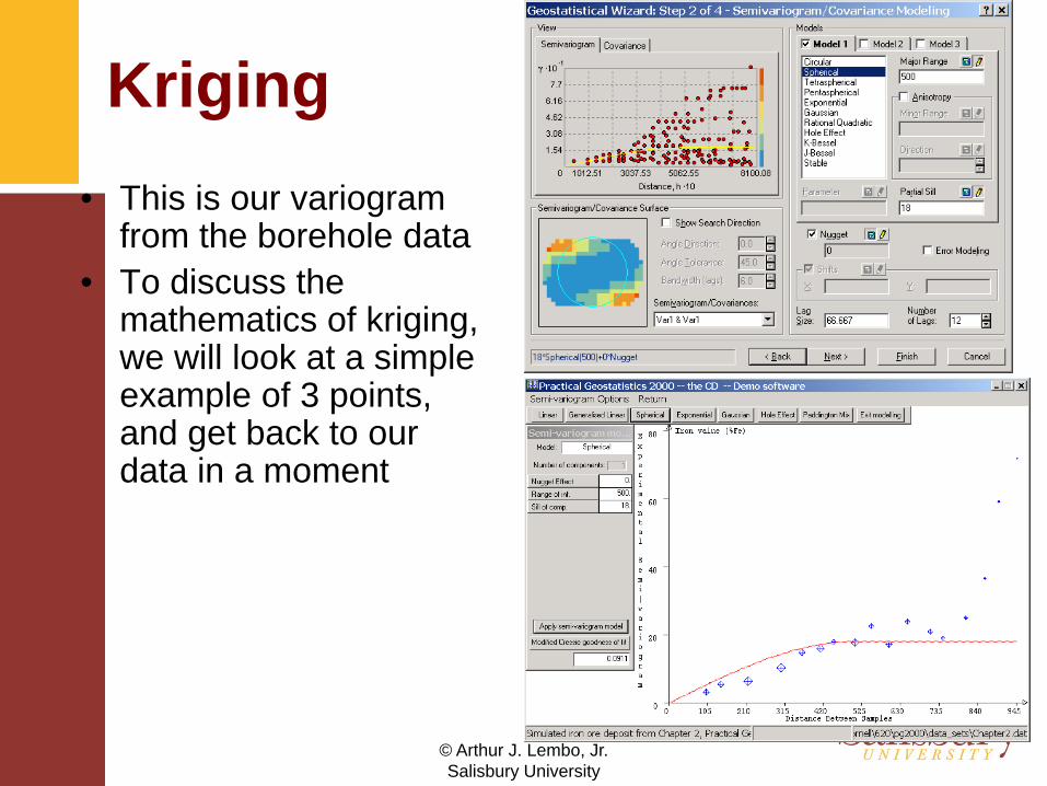
Kriging• This is our variogram

from the borehole data• To discuss the

mathematics of kriging, we will look at a simple example of 3 points, and get back to our data in a moment


Kriging

Numerical Exampleof Iron Ore Data

From Practical Geostatistics 2000


Data Set• Iron Ore Data, based on sample

set from PG 2000• Three point example for

simplicity


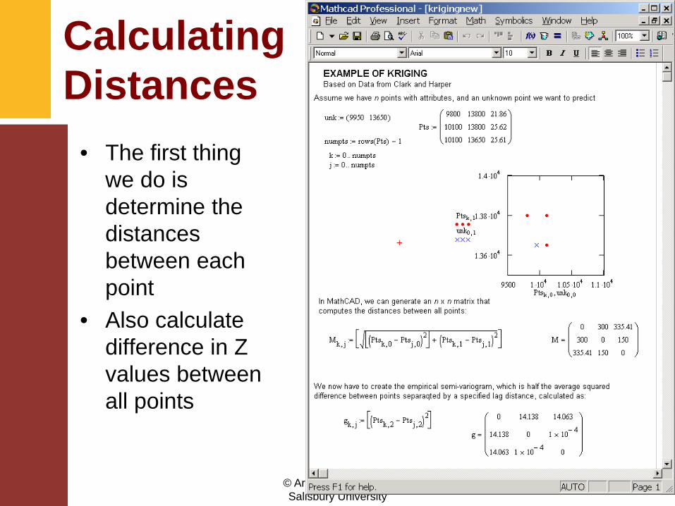
Calculating Distances

• The first thing we do is determine the distances between each point

• Also calculate difference in Z values between all points


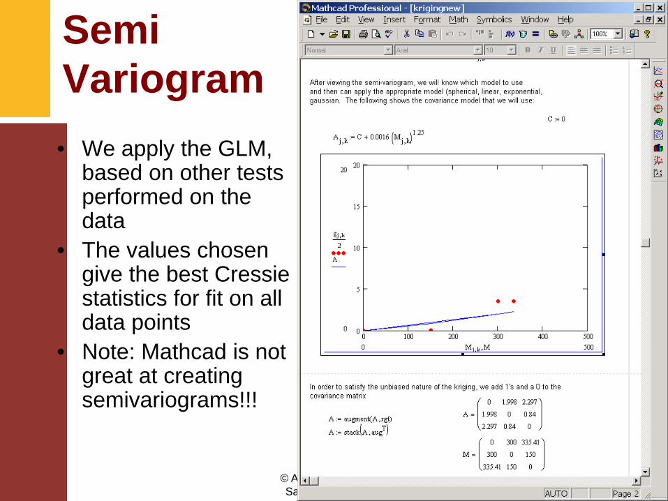
Semi Variogram• We apply the GLM,

based on other tests performed on the data

• The values chosen give the best Cressie statistics for fit on all data points

• Note: Mathcad is not great at creating semivariograms!!!


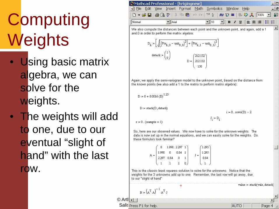
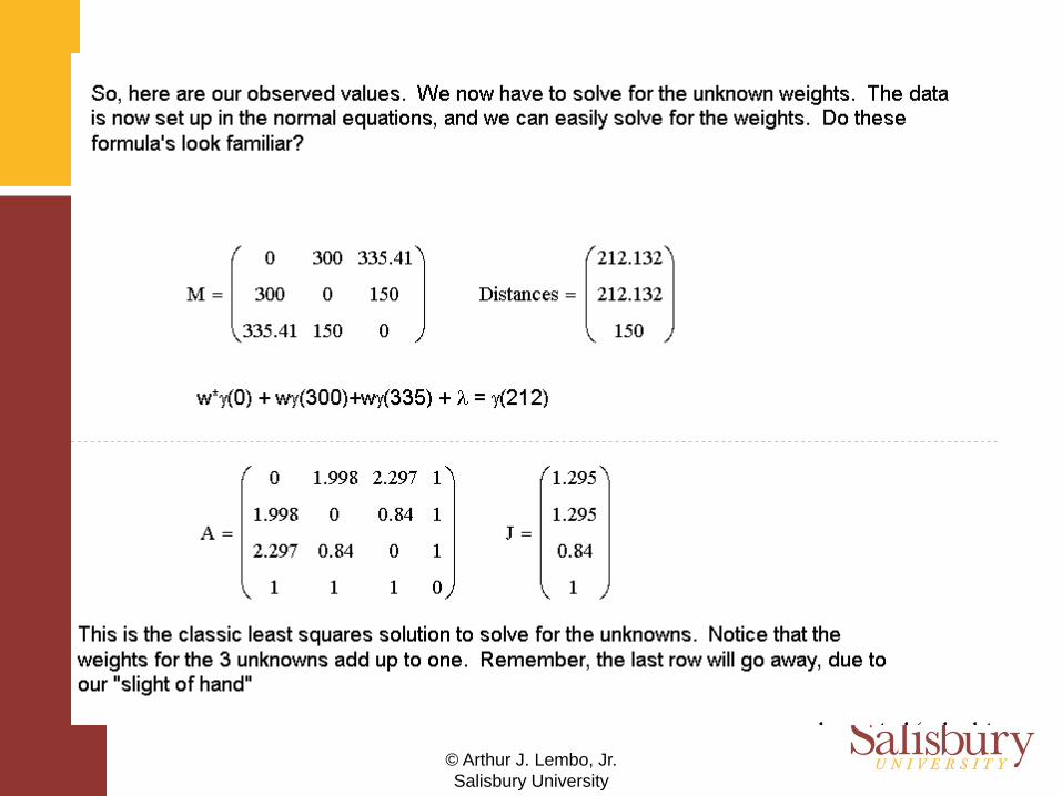
ComputingWeights• Using basic matrix

algebra, we can solve for the weights.

• The weights will add to one, due to our eventual “slight of hand” with the last row.


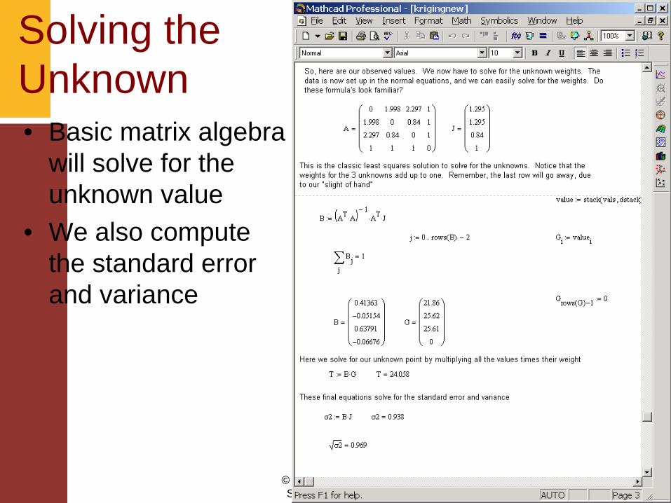
Solving theUnknown• Basic matrix algebra

will solve for the unknown value

• We also compute the standard error and variance


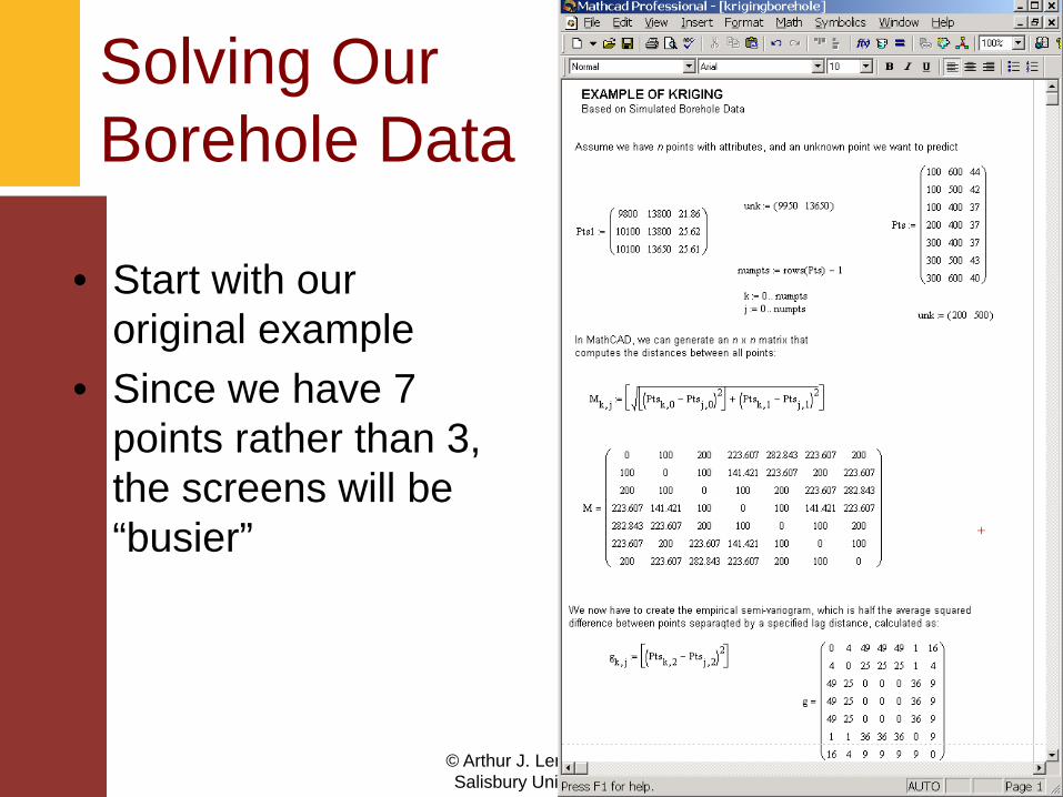
Solving OurBorehole Data

• Start with our original example

• Since we have 7 points rather than 3, the screens will be “busier”


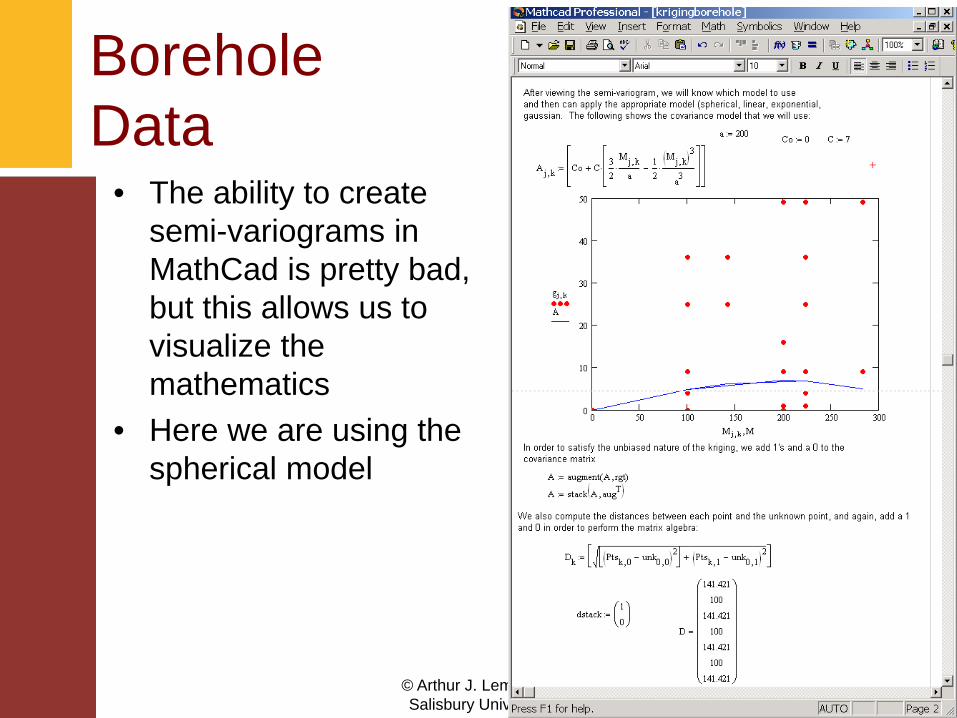
Borehole Data

• The ability to create semi-variograms in MathCad is pretty bad, but this allows us to visualize the mathematics

• Here we are using the spherical model


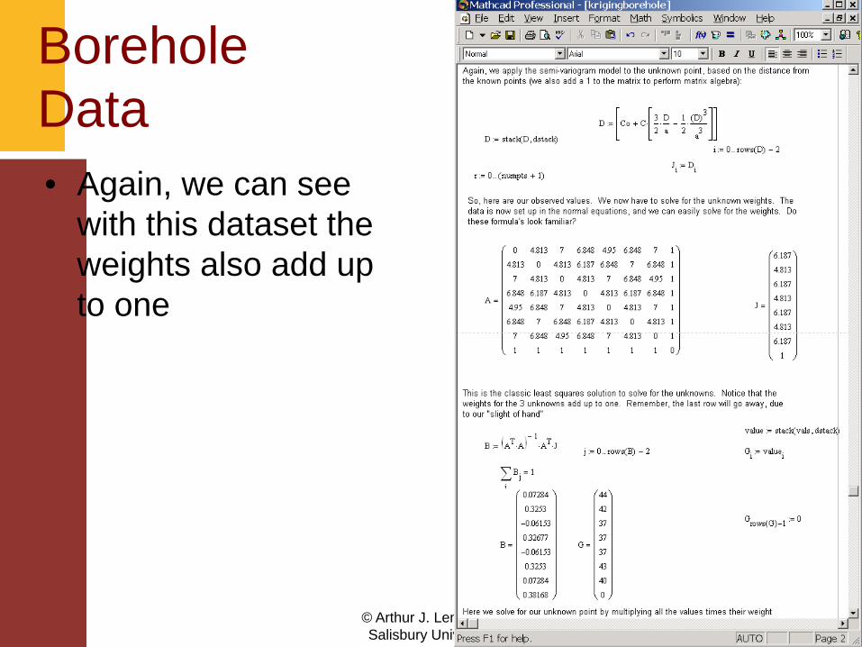
Borehole Data• Again, we can see

with this dataset the weights also add up to one


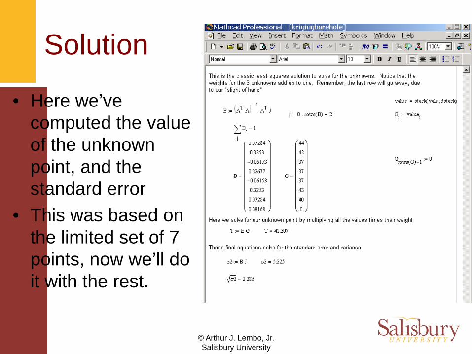
Solution

• Here we’ve computed the value of the unknown point, and the standard error

• This was based on the limited set of 7 points, now we’ll do it with the rest.


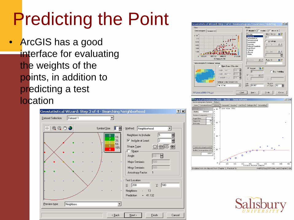
Predicting the Point• ArcGIS has a good

interface for evaluating the weights of the points, in addition to predicting a test location


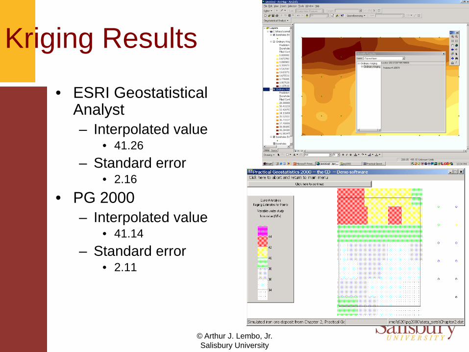
Kriging Results

• ESRI Geostatistical Analyst– Interpolated value

• 41.26– Standard error

• 2.16

• PG 2000– Interpolated value

• 41.14– Standard error

• 2.11


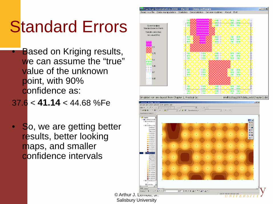
Standard Errors• Based on Kriging results,

we can assume the “true” value of the unknown point, with 90% confidence as:

37.6 < 41.14 < 44.68 %Fe

• So, we are getting better results, better looking maps, and smaller confidence intervals


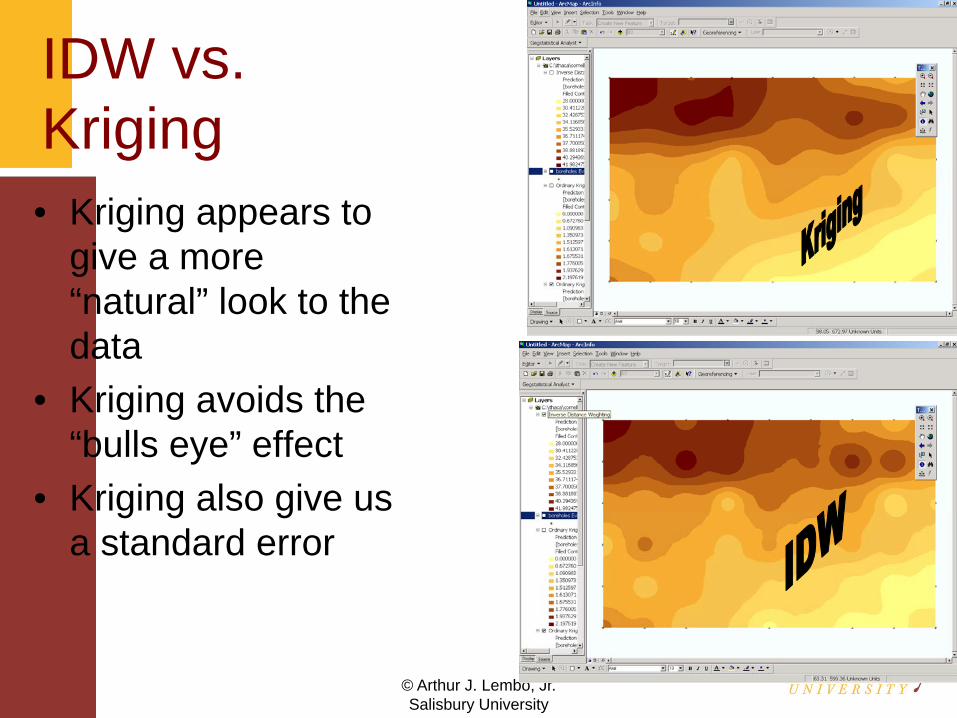
IDW vs. Kriging• Kriging appears to

give a more “natural” look to the data

• Kriging avoids the “bulls eye” effect

• Kriging also give us a standard error


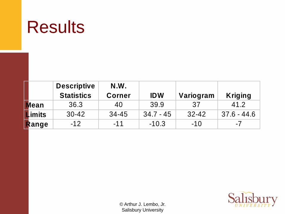
Results

Descriptive Statistics

N.W. Corner IDW Variogram Kriging

Mean 36.3 40 39.9 37 41.2Limits 30-42 34-45 34.7 - 45 32-42 37.6 - 44.6Range -12 -11 -10.3 -10 -7


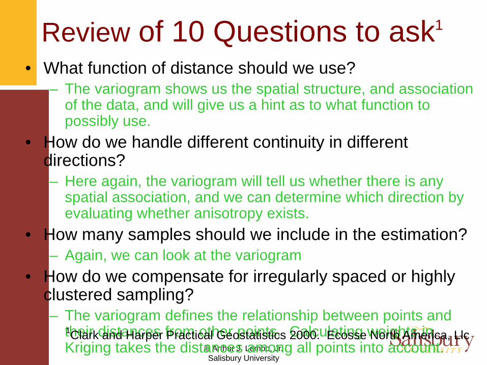
Review of 10 Questions to ask1

• What function of distance should we use?– The variogram shows us the spatial structure, and association

of the data, and will give us a hint as to what function to possibly use.

• How do we handle different continuity in different directions?– Here again, the variogram will tell us whether there is any

spatial association, and we can determine which direction by evaluating whether anisotropy exists.

• How many samples should we include in the estimation?– Again, we can look at the variogram

• How do we compensate for irregularly spaced or highly clustered sampling?– The variogram defines the relationship between points and

their distances from other points. Calculating weights in Kriging takes the distances among all points into account. 1Clark and Harper Practical Geostatistics 2000. Ecosse North America, Llc


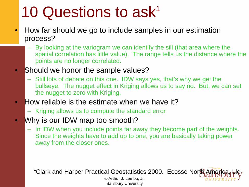
10 Questions to ask1

• How far should we go to include samples in our estimation process?– By looking at the variogram we can identify the sill (that area where the

spatial correlation has little value). The range tells us the distance where the points are no longer correlated.

• Should we honor the sample values?– Still lots of debate on this one. IDW says yes, that’s why we get the

bullseye. The nugget effect in Kriging allows us to say no. But, we can set the nugget to zero with Kriging.

• How reliable is the estimate when we have it?– Kriging allows us to compute the standard error

• Why is our IDW map too smooth?– In IDW when you include points far away they become part of the weights.

Since the weights have to add up to one, you are basically taking power away from the closer ones.

1Clark and Harper Practical Geostatistics 2000. Ecosse North America, Llc


10 Questions to Ask

•What happens if our sample data is not Normal?–Basically, make the data normal…

•What happens if there is a strong trend in the values?

–First, remove the trend, then re-interpolate the points (see ESRI Calif. Ozone example, or Clark and Harper Wolfcamp Data)


Conclusions• It is possible to interpolate an unknown point

based on other points in a data set• While it can be done with descriptive

statistics, other methods are clearly better• The variogram helps answer many questions

related to our data, and provides a wealth of information related to the spatial structure of the data

• More robust (geostatistical) methods for interpolation appear to provide better results

spatial interpolation - salisbury universityspatial interpolation inverse distance weighting the...

Documents