spatial patterns in stage-structured populations with...
TRANSCRIPT

Spatial Patterns in Stage-StructuredPopulations with Density Dependent Dispersal
Item Type text; Electronic Dissertation
Authors Robertson, Suzanne Lora
Publisher The University of Arizona.
Rights Copyright © is held by the author. Digital access to this materialis made possible by the University Libraries, University of Arizona.Further transmission, reproduction or presentation (such aspublic display or performance) of protected items is prohibitedexcept with permission of the author.
Download date 08/07/2018 23:27:36
Link to Item http://hdl.handle.net/10150/194472
Spatial Patterns in Stage-Structured
Populations with Density Dependent Dispersal
by
Suzanne Lora Robertson
A Dissertation Submitted to the Faculty of the
Graduate Interdisciplinary Programin Applied Mathematics
In Partial Fulfillment of the RequirementsFor the Degree of
Doctor of Philosophy
In the Graduate College
The University of Arizona
2 0 0 9
2
THE UNIVERSITY OF ARIZONAGRADUATE COLLEGE
As members of the Final Examination Committee, we certify that we have read thedissertation prepared by Suzanne Lora Robertson entitledSpatial Patterns in Stage-Structured Populations with Density
Dependent Dispersal
and recommend that it be accepted as fulfilling the dissertation requirement for theDegree of Doctor of Philosophy.
Date: 24 April 2009
J. M. Cushing
Date: 24 April 2009
Michael Tabor
Date: 24 April 2009
Joseph Watkins
Final approval and acceptance of this dissertation is contingent upon the candidate’ssubmission of the final copies of the dissertation to the Graduate College.
I hereby certify that I have read this dissertation prepared under my direction andrecommend that it be accepted as fulfilling the dissertation requirement.
Date: 24 April 2009
Dissertation Director: J. M. Cushing

3
STATEMENT BY AUTHOR
This dissertation has been submitted in partial fulfillment of requirements for anadvanced degree at The University of Arizona and is deposited in the UniversityLibrary to be made available to borrowers under rules of the Library.
Brief quotations from this dissertation are allowable without special permission,provided that accurate acknowledgment of source is made. Requests for permissionfor extended quotation from or reproduction of this manuscript in whole or in partmay be granted by the head of the major department or the Dean of the GraduateCollege when in his or her judgment the proposed use of the material is in the interestsof scholarship. In all other instances, however, permission must be obtained from theauthor.
SIGNED: Suzanne Lora Robertson

4
Acknowledgments
I would like to thank my advisor, Jim Cushing, for being a wonderful mentor. Hehas taught me so much and I am grateful for the opportunity to work with him.
Thanks to my committee members, Joseph Watkins and Michael Tabor, for all oftheir professional guidance and support during my time as a graduate student.
I am grateful to Bob Costantino for providing much of the biological data for thiswork and for his insight during our many research discussions.
I gratefully acknowledge Shandelle Henson, my undergraduate mentor, for inspiringme to pursue a graduate degree in Applied Mathematics.
Finally, I wish to thank my family and friends for their love and encouragement.

5
Dedication
For Mom

6
Table of Contents
List of Figures . . . . . . . . . . . . . . . . . . . . . . . . . . . . . . . . . 8
List of Tables . . . . . . . . . . . . . . . . . . . . . . . . . . . . . . . . . . 11
Abstract . . . . . . . . . . . . . . . . . . . . . . . . . . . . . . . . . . . . . 12
Chapter 1. Introduction . . . . . . . . . . . . . . . . . . . . . . . . . . 13
1.1. Life Cycle Stage Interactions and Spatial Structure . . . . . . . . . . 131.2. Life Cycle Stages and Spatial Patterns in Flour Beetles . . . . . . . . 15
1.2.1. Tribolium castaneum and Tribolium confusum . . . . . . . . . 151.2.2. Tribolium brevicornis . . . . . . . . . . . . . . . . . . . . . . . 16
1.3. Density Dependent Dispersal . . . . . . . . . . . . . . . . . . . . . . . 221.4. Spatial Models and Prior Investigations . . . . . . . . . . . . . . . . . 23
Chapter 2. A Bifurcation Analysis of Stage-StructuredDensity-Dependent Integrodifference Equations . . . . . . . . . 28
2.1. Definitions and Preliminaries . . . . . . . . . . . . . . . . . . . . . . . 292.2. Model Development and Existence of Equilibria . . . . . . . . . . . . 312.3. Equilibrium Stability . . . . . . . . . . . . . . . . . . . . . . . . . . . 37
2.3.1. Extinction Equilibrium . . . . . . . . . . . . . . . . . . . . . . 372.3.2. Stability and Direction of Bifurcation . . . . . . . . . . . . . . 38
2.4. Examples of Bifurcation Theory . . . . . . . . . . . . . . . . . . . . . 402.4.1. Example 1: Uniform dispersal . . . . . . . . . . . . . . . . . . 402.4.2. Example 2: Spatially dependent dispersal . . . . . . . . . . . . 442.4.3. Example 3: A more complex spatially dependent kernel . . . . 47
2.5. Appendix . . . . . . . . . . . . . . . . . . . . . . . . . . . . . . . . . 512.5.1. The Krein-Rutman Theorem . . . . . . . . . . . . . . . . . . . 512.5.2. Relationship between n and λ0 . . . . . . . . . . . . . . . . . 512.5.3. Compactness of T + nΦ . . . . . . . . . . . . . . . . . . . . . 53
Chapter 3. Juvenile-Adult (Toy) Models . . . . . . . . . . . . . . . 55
3.1. Hostile Boundary Conditions . . . . . . . . . . . . . . . . . . . . . . . 563.1.1. Application of Theory . . . . . . . . . . . . . . . . . . . . . . 63
3.2. Mixed Boundary Conditions . . . . . . . . . . . . . . . . . . . . . . . 663.3. Role of Domain Size . . . . . . . . . . . . . . . . . . . . . . . . . . . 69
Table of Contents—Continued
7
Chapter 4. Case Studies Using Models for Flour Beetles (Tri-
bolium) . . . . . . . . . . . . . . . . . . . . . . . . . . . . . . . . . . . . . 73
4.1. Spatial Patterns in Tribolium castaneum . . . . . . . . . . . . . . . . 734.1.1. The LPA Model . . . . . . . . . . . . . . . . . . . . . . . . . 734.1.2. The Spatial LPA Model . . . . . . . . . . . . . . . . . . . . . 74
4.2. Spatial Patterns in Tribolium brevicornis . . . . . . . . . . . . . . . . 784.2.1. The SLPA Model . . . . . . . . . . . . . . . . . . . . . . . . 794.2.2. Parametrization . . . . . . . . . . . . . . . . . . . . . . . . . . 814.2.3. The Spatial SLPA Model . . . . . . . . . . . . . . . . . . . . 85
Chapter 5. Concluding Remarks . . . . . . . . . . . . . . . . . . . . . 100
5.1. Future Investigations . . . . . . . . . . . . . . . . . . . . . . . . . . . 105
References . . . . . . . . . . . . . . . . . . . . . . . . . . . . . . . . . . . . 108
8
List of Figures
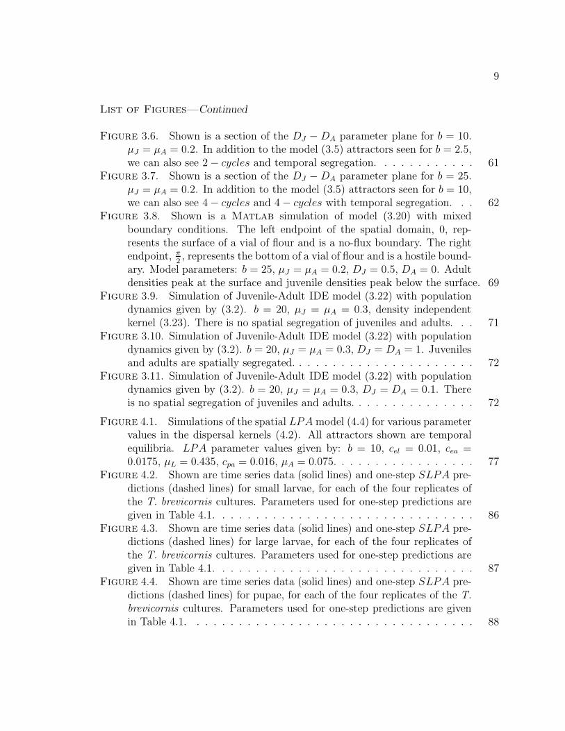
Figure 1.1. Data from Ghent [14]. 0 represents the surface of the vial and 1represents the bottom. . . . . . . . . . . . . . . . . . . . . . . . . . . . . 18
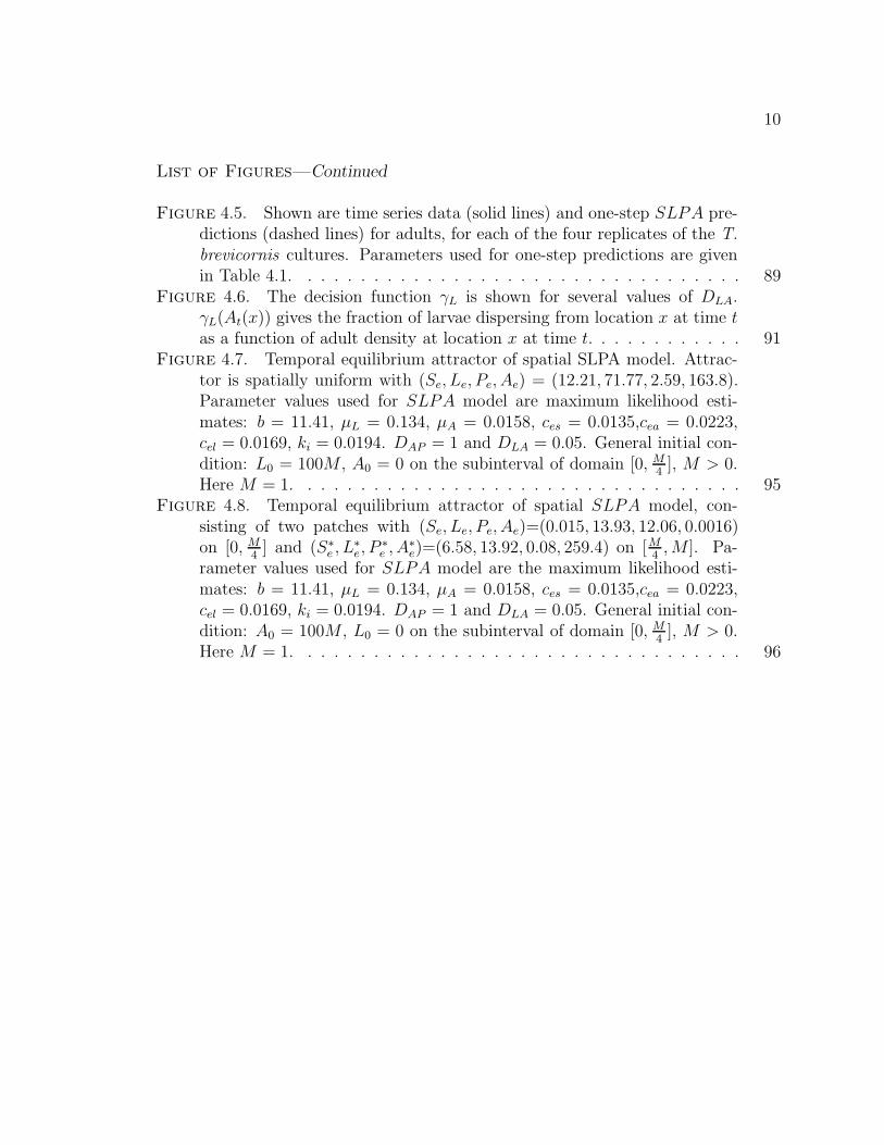
Figure 1.2. Cultures of T. brevicornis showing segregation of adults andother life stages. Photo 1.2b by R. F. Costantino. . . . . . . . . . . . . . 19
Figure 1.3. Aerial view of Tribolium castaneum adults on surface of rectan-gular box of flour. There are some adults near the edges of the box butno distinct pattern or segregation of life cycle stages. . . . . . . . . . . . 20
Figure 1.4. Aerial view of Tribolium brevicornis. Each of three rows showsegregation of adults and pupae, illustrating the pupal nest on the left.Each row was started with large larvae and adults on the left side. Theywere restrained in this subhabitat for 6 weeks, then a panel was removedand they were allowed to disperse throughout the entire row. This photowas taken a week after the door was opened. Photo by R. F. Costantino. 20
Figure 1.5. New callow adults emerging from nest in (b) indicate large larvaereturn to nest to pupate. Photos are 6 weeks apart. Photos by R. F.Costantino. . . . . . . . . . . . . . . . . . . . . . . . . . . . . . . . . . . 21
Figure 1.6. Aerial view of Tribolium brevicornis. Doors are open at ends ofrows to allow beetles to move throughout entire box. Culture started with100 adults at upper right corner, immediately permitted to disperse. Nopupal nest is established. . . . . . . . . . . . . . . . . . . . . . . . . . . 21
Figure 3.1. Time-equilibrium attractor of Juvenile-Adult IDE model (3.5).b = 25, µL = µA = 0.2. There is no density dependence in the dispersalkernels: DJ = DA = 0 . . . . . . . . . . . . . . . . . . . . . . . . . . . . 58
Figure 3.2. Time-equilibrium attractor for Juvenile-Adult IDE model (3.5),showing spatial segregation of juveniles and adults. b = 25, µL = µA =0.2. DJ = 0.5, DA = 0. . . . . . . . . . . . . . . . . . . . . . . . . . . . 59
Figure 3.3. 2-cycle attractor of Juvenile-Adult IDE model (3.5), with tem-poral segregation of juveniles and adults. b = 25, µL = µA = 0.2. DJ = 0,DA = 0.5 . . . . . . . . . . . . . . . . . . . . . . . . . . . . . . . . . . . 59
Figure 3.4. 4-cycle attractor of Juvenile-Adult IDE model (3.5), with tem-poral segregation of juveniles and adults. b = 25, µL = µA = 0.2.DJ = DA = 0.5 . . . . . . . . . . . . . . . . . . . . . . . . . . . . . . . 60
Figure 3.5. Shown is a section of the DJ − DA parameter plane for b = 2.5.µJ = µA = 0.2. We look at 0 ≤ DJ ≤ 1 and 0 ≤ DA ≤ 1. Allcombinations of DJ and DA in this range result in equilibrium dynamicsfor model (3.5). Spatial segregation is possible for large enough DJ andsmall enough DA. . . . . . . . . . . . . . . . . . . . . . . . . . . . . . . 61
List of Figures—Continued
9
Figure 3.6. Shown is a section of the DJ − DA parameter plane for b = 10.µJ = µA = 0.2. In addition to the model (3.5) attractors seen for b = 2.5,we can also see 2 − cycles and temporal segregation. . . . . . . . . . . . 61
Figure 3.7. Shown is a section of the DJ − DA parameter plane for b = 25.µJ = µA = 0.2. In addition to the model (3.5) attractors seen for b = 10,we can also see 4 − cycles and 4 − cycles with temporal segregation. . . 62
Figure 3.8. Shown is a Matlab simulation of model (3.20) with mixedboundary conditions. The left endpoint of the spatial domain, 0, rep-resents the surface of a vial of flour and is a no-flux boundary. The rightendpoint, π
2, represents the bottom of a vial of flour and is a hostile bound-
ary. Model parameters: b = 25, µJ = µA = 0.2, DJ = 0.5, DA = 0. Adultdensities peak at the surface and juvenile densities peak below the surface. 69
Figure 3.9. Simulation of Juvenile-Adult IDE model (3.22) with populationdynamics given by (3.2). b = 20, µJ = µA = 0.3, density independentkernel (3.23). There is no spatial segregation of juveniles and adults. . . 71
Figure 3.10. Simulation of Juvenile-Adult IDE model (3.22) with populationdynamics given by (3.2). b = 20, µJ = µA = 0.3, DJ = DA = 1. Juvenilesand adults are spatially segregated. . . . . . . . . . . . . . . . . . . . . . 72
Figure 3.11. Simulation of Juvenile-Adult IDE model (3.22) with populationdynamics given by (3.2). b = 20, µJ = µA = 0.3, DJ = DA = 0.1. Thereis no spatial segregation of juveniles and adults. . . . . . . . . . . . . . . 72
Figure 4.1. Simulations of the spatial LPA model (4.4) for various parametervalues in the dispersal kernels (4.2). All attractors shown are temporalequilibria. LPA parameter values given by: b = 10, cel = 0.01, cea =0.0175, µL = 0.435, cpa = 0.016, µA = 0.075. . . . . . . . . . . . . . . . . 77
Figure 4.2. Shown are time series data (solid lines) and one-step SLPA pre-dictions (dashed lines) for small larvae, for each of the four replicates ofthe T. brevicornis cultures. Parameters used for one-step predictions aregiven in Table 4.1. . . . . . . . . . . . . . . . . . . . . . . . . . . . . . . 86
Figure 4.3. Shown are time series data (solid lines) and one-step SLPA pre-dictions (dashed lines) for large larvae, for each of the four replicates ofthe T. brevicornis cultures. Parameters used for one-step predictions aregiven in Table 4.1. . . . . . . . . . . . . . . . . . . . . . . . . . . . . . . 87
Figure 4.4. Shown are time series data (solid lines) and one-step SLPA pre-dictions (dashed lines) for pupae, for each of the four replicates of the T.
brevicornis cultures. Parameters used for one-step predictions are givenin Table 4.1. . . . . . . . . . . . . . . . . . . . . . . . . . . . . . . . . . 88
List of Figures—Continued
10
Figure 4.5. Shown are time series data (solid lines) and one-step SLPA pre-dictions (dashed lines) for adults, for each of the four replicates of the T.
brevicornis cultures. Parameters used for one-step predictions are givenin Table 4.1. . . . . . . . . . . . . . . . . . . . . . . . . . . . . . . . . . 89
Figure 4.6. The decision function γL is shown for several values of DLA.γL(At(x)) gives the fraction of larvae dispersing from location x at time tas a function of adult density at location x at time t. . . . . . . . . . . . 91
Figure 4.7. Temporal equilibrium attractor of spatial SLPA model. Attrac-tor is spatially uniform with (Se, Le, Pe, Ae) = (12.21, 71.77, 2.59, 163.8).Parameter values used for SLPA model are maximum likelihood esti-mates: b = 11.41, µL = 0.134, µA = 0.0158, ces = 0.0135,cea = 0.0223,cel = 0.0169, ki = 0.0194. DAP = 1 and DLA = 0.05. General initial con-dition: L0 = 100M , A0 = 0 on the subinterval of domain [0, M
4], M > 0.
Here M = 1. . . . . . . . . . . . . . . . . . . . . . . . . . . . . . . . . . 95Figure 4.8. Temporal equilibrium attractor of spatial SLPA model, con-
sisting of two patches with (Se, Le, Pe, Ae)=(0.015, 13.93, 12.06, 0.0016)on [0, M
4] and (S∗
e , L∗e, P
∗e , A∗
e)=(6.58, 13.92, 0.08, 259.4) on [M4, M ]. Pa-
rameter values used for SLPA model are the maximum likelihood esti-mates: b = 11.41, µL = 0.134, µA = 0.0158, ces = 0.0135,cea = 0.0223,cel = 0.0169, ki = 0.0194. DAP = 1 and DLA = 0.05. General initial con-dition: A0 = 100M , L0 = 0 on the subinterval of domain [0, M
4], M > 0.
Here M = 1. . . . . . . . . . . . . . . . . . . . . . . . . . . . . . . . . . 96

11
List of Tables
Table 4.1. Maximum likelihood parameter estimates for the stochastic SLPAmodel (4.8). . . . . . . . . . . . . . . . . . . . . . . . . . . . . . . . . . 85
Table 4.2. Residual Analysis. Means and variances for the square root resid-uals for stages S, L, P and A. Untransformed residuals can be seen inFigures 4.2-4.5, as the difference between the model prediction and ob-served stage vector at each time-step. Maximum likelihood estimates forthe variances of the transformed residuals are given in Table 4.1. . . . . 90
Table 4.3. Comparison of population vectors and total population size forspatially uniform versus spatially segregated (patchy) attractors for vary-ing degrees of inhibition on the spatial domain [0, 1]. All other parametervalues used were: b = 11.41, µL = 0.134, µA = 0.0158, ces = 0.0135,cea =0.0223, cel = 0.0169, DAP = 1 and DLA = 0.05. Simulations with initialcondition a were started with 25 large larvae on the left 1
4of the spa-
tial domain (an initial distribution of L0(x) = 100, A0(x) = 0 on [0, 14]).
Each simulation started with this initial condition went to the spatiallyuniform attractor illustrated in Figure 4.7. Simulations with initial con-dition b were started with 25 adults on the left 1
4of the spatial domain
(an initial distribution of L0(x) = 0, A0(x) = 100 on [0, 14]). With the
exception of ki = 0, simulations with initial condition b led to the patchyattractor illustrated in Figure 4.8. For each value of ki, the total numberof small larvae, large larvae, pupae, adults and total population size (thesum of all stages) are calculated for each attractor (by integrating eachequilibrium distribution from 0 to 1 with respect to the spatial variablex). The greater number is shown in bold. . . . . . . . . . . . . . . . . . 94
12
Abstract
Spatial segregation among life cycle stages has been observed in many stage-structured
species, including species of the flour beetle Tribolium. Patterns have been observed
both in homogeneous and heterogeneous environments. We investigate density depen-
dent dispersal of life cycle stages as a mechanism responsible for this separation. By
means of mathematical analysis and numerical simulations, we explore this hypothe-
sis using stage-structured, integrodifference equation (IDE) models that incorporate
density dependent dispersal kernels.
In Chapter 2 we develop a bifurcation theory approach to the existence and sta-
bility of (non-extinction) equilibria for a general class of structured integrodifference
equation models on finite spatial domains with density dependent kernels. We show
that a continuum of such equilibria bifurcates from the extinction equilibrium when it
loses stability as the net reproductive number n increases through 1. We give several
examples to illustrate the theory.
In Chapter 3 we investigate mechanisms that can lead to spatial patterns in two
dimensional Juvenile-Adult IDE models. The bifurcation theory shows that such
patterns do not arise for n near 1. For larger values of n we show, via numerical
simulation, that density dependent dispersal can lead to the segregation of life cycle
stages in the sense that each stage peaks in a different spatial location.
Finally, in Chapter 4, we construct spatial models to describe the population
dynamics of T. castaneum, T. confusum and T. brevicornis and use them to assess
density dependent dispersal mechanisms that are able to explain spatial patterns that
have been observed in these species.
13
Chapter 1
Introduction
1.1 Life Cycle Stage Interactions and Spatial Structure
Spatial dispersal can be an important component that affects the dynamics of popula-
tions. There are many factors that may cause an organism to move between different
spatial locations, including quality of the environment, crowding and competition for
resources (between and within species). If space is not homogenous, mobile organisms
can take advantage of these spatial heterogeneities to develop their own spatial niche.
For example, similar species may prefer slightly different environments or types of
resources. The resulting non-uniform density distribution can allow similar species to
coexist through spatial segregation in situations where one species would otherwise
go extinct (competitive exclusion).
Interactions among life cycle stages may also promote non-uniform spatial struc-
ture. For example, spatial heterogeneities can give cannibalized (prey) stages an
opportunity to seek refuge from the cannibalistic (predator) stages, resulting in the
spatial segregation of life cycle stages. In some cannibalistic species, such as the
freshwater isopod Thermosphaeroma thermophilum [22], there is evidence that the
observed intraspecific habitat segregation is the result of an adaptation to cannibalism
as a stage-specific predation risk rather than other factors such as stage-specific re-
source preferences. Laboratory experiments have shown that juveniles actively avoid
the adults (both sexes, but more so the cannibalistic adult males) by taking advantage

14
of available refuges to keep from being eaten.
Even if spatial refuges are not available, cannibalized stages may still try to avoid
the cannibals. This phenomenon has been observed in the isopod Saduria entomon
[28, 43]. Larger isopods will cannibalize the smaller ones until they reach a critical
size of about 12 mm. Sparrevik and Leonardsson [43] experimentally demonstrated
that the smaller isopods will avoid swimming into an area of water that has passed
through a population of larger isopods, and the severity of the avoidance behavior
increases with the density of the larger conspecifics. Furthermore, a negative cor-
relation between densities of large and small isopods has been found in the field,
indicating that cannibalism (along with density dependent avoidance adaptations)
plays an important role in spatial structure as well as in density regulation for this
species.
The spatial separation of different age classes or life cycle stages has also been
documented in many other cannibalistic species, serving to reduce predation mortal-
ity. A study of the cave-dwelling mysids Hemimysis speluncola [40] found juveniles
near the cave entrance, while adults inhabited the innermost parts of the cave. Juve-
niles of the amphipod species Pallasea quadrispinosa tend to occupy shallow waters
while adults are mainly found in deeper, cooler waters. This is very similar to the
phototactic response noted by Hunte and Myers [20] in gammarid amphipods, which
they hypothesize is an evolutionary adaptation to reduce cannibalism of juveniles by
adults. These examples show heterogeneous environments, together with life cycle
stage interactions, can lead to differences in spatial distributions among conspecifics.
Life cycle stage interactions alone are sometimes sufficient for the formation of
non-uniform spatial distributions, as spatial patterns have also been observed in ho-
mogenous environments with no refuges available. Specifically, spatial segregation of
15
larvae and adults have been documented in the cannibalistic flour beetles Tribolium
confusum, T. castaneum, and T. brevicornis in homogeneous habitats of flour. While
cannibalism can be a mechanism that drives spatial segregation of life cycle stages,
other types of density dependent inter-stage interactions can also play a role. For
example, for one species of Tribolium, density related larval inhibition by adults can
enhance spatial patterns, as we will see in section 1.2 and in Chapter 4.
1.2 Life Cycle Stages and Spatial Patterns in Flour Beetles
1.2.1 Tribolium castaneum and Tribolium confusum
The flour beetle (genus Tribolium) progresses through four stages over the course of
its life cycle: egg, larva, pupa, and adult. Spatial patterns have been observed in
several species of flour beetles in which the larval and adult stages are mobile and can
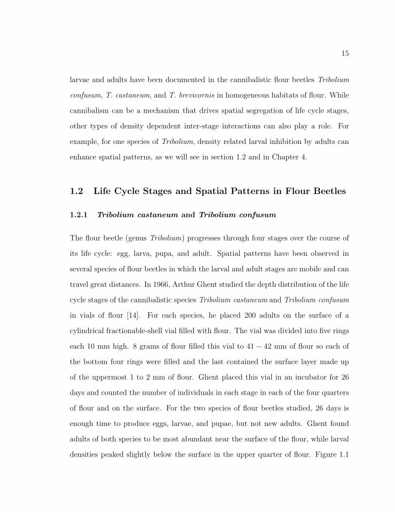
travel great distances. In 1966, Arthur Ghent studied the depth distribution of the life
cycle stages of the cannibalistic species Tribolium castaneum and Tribolium confusum
in vials of flour [14]. For each species, he placed 200 adults on the surface of a
cylindrical fractionable-shell vial filled with flour. The vial was divided into five rings
each 10 mm high. 8 grams of flour filled this vial to 41 − 42 mm of flour so each of
the bottom four rings were filled and the last contained the surface layer made up
of the uppermost 1 to 2 mm of flour. Ghent placed this vial in an incubator for 26
days and counted the number of individuals in each stage in each of the four quarters
of flour and on the surface. For the two species of flour beetles studied, 26 days is
enough time to produce eggs, larvae, and pupae, but not new adults. Ghent found
adults of both species to be most abundant near the surface of the flour, while larval
densities peaked slightly below the surface in the upper quarter of flour. Figure 1.1
16
shows the observed depth distributions for various life stages of Tribolium castaneum
and Tribolium confusum. We note that surface patterns involving the segregation
of juveniles and adults have not been observed in T. castaneum or T. confusum,
although Neyman, Park and Scott [37] documented a general trend of increasing
density of adults towards the edges of a square container (and along edges towards
the corners).
1.2.2 Tribolium brevicornis
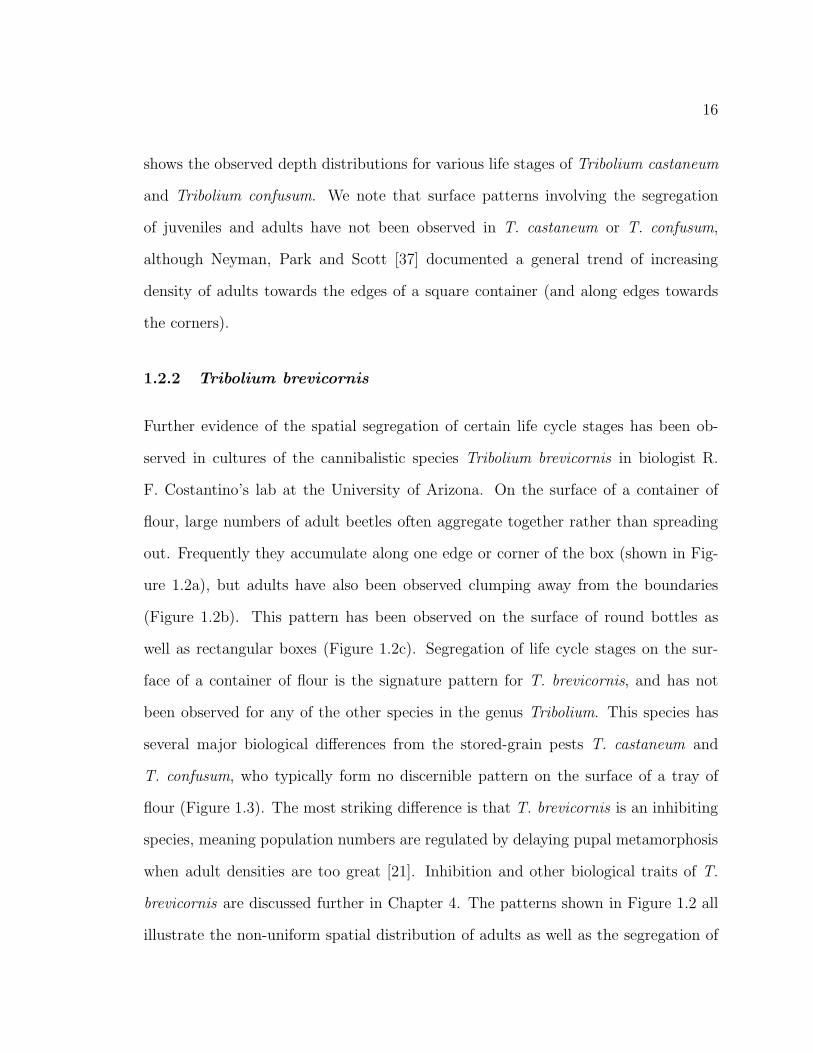
Further evidence of the spatial segregation of certain life cycle stages has been ob-
served in cultures of the cannibalistic species Tribolium brevicornis in biologist R.
F. Costantino’s lab at the University of Arizona. On the surface of a container of
flour, large numbers of adult beetles often aggregate together rather than spreading
out. Frequently they accumulate along one edge or corner of the box (shown in Fig-
ure 1.2a), but adults have also been observed clumping away from the boundaries
(Figure 1.2b). This pattern has been observed on the surface of round bottles as
well as rectangular boxes (Figure 1.2c). Segregation of life cycle stages on the sur-
face of a container of flour is the signature pattern for T. brevicornis, and has not
been observed for any of the other species in the genus Tribolium. This species has
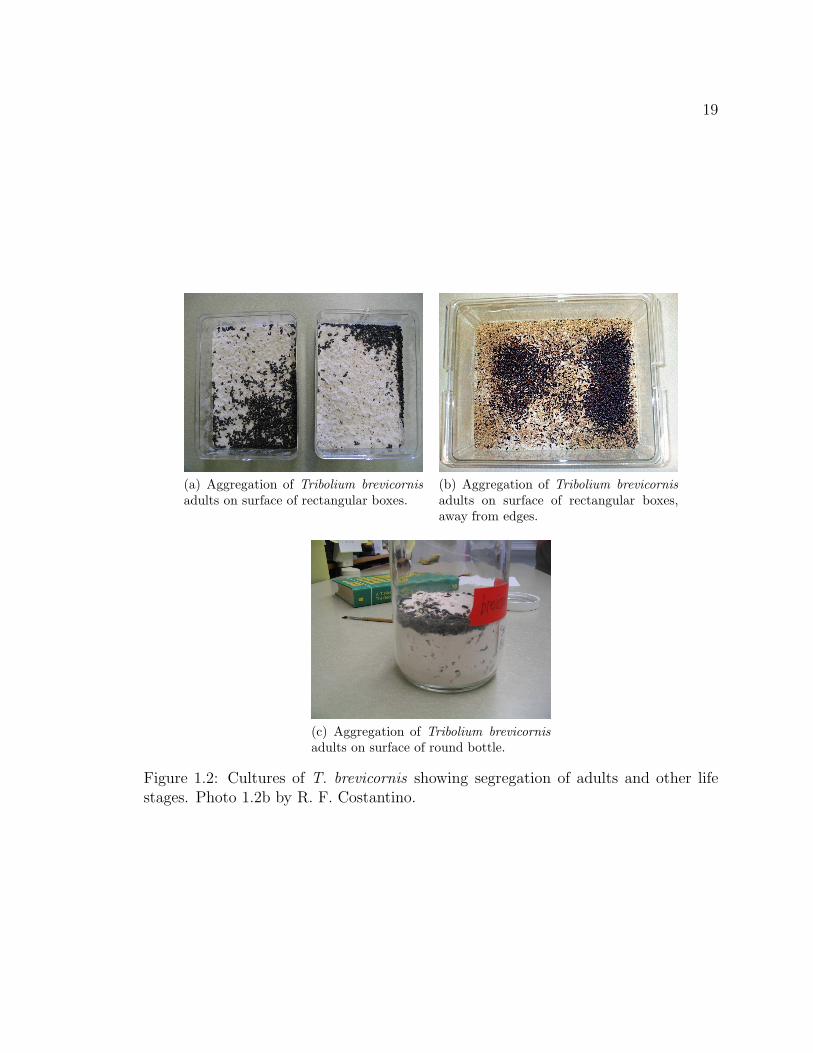
several major biological differences from the stored-grain pests T. castaneum and
T. confusum, who typically form no discernible pattern on the surface of a tray of
flour (Figure 1.3). The most striking difference is that T. brevicornis is an inhibiting
species, meaning population numbers are regulated by delaying pupal metamorphosis
when adult densities are too great [21]. Inhibition and other biological traits of T.
brevicornis are discussed further in Chapter 4. The patterns shown in Figure 1.2 all
illustrate the non-uniform spatial distribution of adults as well as the segregation of

17
adults and other life stages. However, the specific location of the adults varies greatly
among cultures, even among containers of the same size and shape.
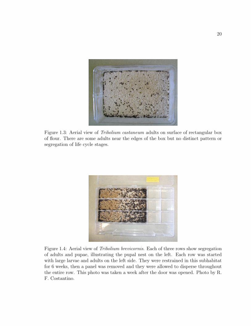
In one container, Costantino noticed that patterns were more reproducible than in
the containers shown in Figure 1.2. He used a box similar in size to the one in Figure
1.2b, but that could be subdivided into smaller rectangles by inserting removable
panels. Figure 1.4 shows three replicates of cultures in domains with about two-
thirds the length as those in Figure 1.2b but only about a quarter of the width. We
see the formation of a pupal “nest” on the left side of each of the three rows. Figure
1.5 provides evidence that this pupal nest persists over time. Figure 1.5b was taken
6 weeks after Figure 1.5a, and new callow (light brown) adults can be seen emerging
from the pupal nest, indicating large larvae return there to pupate. The pupal nest
is not seen in all cultures of T. brevicornis. Rather, the pattern formed depends on
the initial condition of the culture and whether the pupal nest has had a chance to
establish itself before widespread dispersal takes place. Figure 1.6 shows a culture of
T. brevicornis in which a pupal nest was never established and exhibits no surface
pattern.

18
0 1/4 1/2 3/4 10
20
40
60
80
100
120
Space
AdultsLarvaePrepupaePupae
(a) Depth distribution of larvae, pre-pupae, pupae and adults in Tribolium
castaneum.
0 1/4 1/2 3/4 10
10
20
30
40
50
60
70
80
90
Space
AdultsLarvae
(b) Depth distribution of larvae and adults in Tribolium confusum.
Figure 1.1: Data from Ghent [14]. 0 represents the surface of the vial and 1 representsthe bottom.
19
(a) Aggregation of Tribolium brevicornis
adults on surface of rectangular boxes.(b) Aggregation of Tribolium brevicornis
adults on surface of rectangular boxes,away from edges.
(c) Aggregation of Tribolium brevicornis
adults on surface of round bottle.
Figure 1.2: Cultures of T. brevicornis showing segregation of adults and other lifestages. Photo 1.2b by R. F. Costantino.
20
Figure 1.3: Aerial view of Tribolium castaneum adults on surface of rectangular boxof flour. There are some adults near the edges of the box but no distinct pattern orsegregation of life cycle stages.
Figure 1.4: Aerial view of Tribolium brevicornis. Each of three rows show segregationof adults and pupae, illustrating the pupal nest on the left. Each row was startedwith large larvae and adults on the left side. They were restrained in this subhabitatfor 6 weeks, then a panel was removed and they were allowed to disperse throughoutthe entire row. This photo was taken a week after the door was opened. Photo by R.F. Costantino.

21
(a)
(b) Six weeks after (a)
Figure 1.5: New callow adults emerging from nest in (b) indicate large larvae returnto nest to pupate. Photos are 6 weeks apart. Photos by R. F. Costantino.
Figure 1.6: Aerial view of Tribolium brevicornis. Doors are open at ends of rowsto allow beetles to move throughout entire box. Culture started with 100 adults atupper right corner, immediately permitted to disperse. No pupal nest is established.
22
1.3 Density Dependent Dispersal
Many stage-structured species have density dependent dispersal mechanisms. For
example, aphid larvae can develop into one of two adult morphs - winged or wingless.
The ability to fly aids in dispersal of the population. Studies have shown that the
proportion of adults having the winged morph is density dependent, depending on
the number of tactile encounters larvae have with other aphids [17]. Density may
also affect the proportion of winged adults with the ability to fly. Another example
of a polymorphism affecting dispersal ability is wing length in the brown planthopper
Nilaparvata lugens [24]. Nymphs developing under crowded conditions leads to a
greater fraction of long-winged adults.
The above examples provide evidence that density can affect the proportion of
a population able to disperse and the degree of dispersal ability. In sections 1.1
and 1.2 we noted some experimental evidence for the density dependent avoidance
of cannibals by the cannibalized stages in stage-structured species, showing density
can affect the locations to which individuals disperse. In this dissertation I will use
certain types of models for the dynamics of structured populations to explore the role
of density dependent dispersal as a mechanism for the spatial segregation of life cycle
stages. I will focus on observed spatial patterns in species of Tribolium for which we
believe density dependent dispersal is the main causal mechanism.
There is substantial evidence that density plays a role in the dispersal of both
T. castaneum and T. confusum [33, 48]. Naylor documented an inter-stage density
dependent avoidance response in T. confusum [34]. When presented with a choice
between unoccupied flour and flour occupied by medium-sized larvae, adult females
tended to choose the unoccupied flour. Furthermore, the number of adults found

23
in vials of flour decreased with increasing larval density. Naylor also observed larvae
leaving crowded vials of flour with high larval densities. The tendency of T. confusum
to move to locations of unoccupied flour over occupied flour was also observed by
Naylor [32].
Further evidence of the avoidance of larvae by adults comes from an experiment
conducted by Prus [38] to look at emigration ability and surface numbers of adult
beetles of different strains and sexes. All cultures were composed of a single sex
of adults, except for one replicate where several males accidentally were mixed in a
culture of females. This resulted in the appearance of larvae, and a notable increase in
the surface numbers and emigration ability of this replicate [38]. Later investigations
confirmed the effect of the presence of larvae in increasing adult surface numbers. In
adult only cultures, the intensity of emigration was found to depend on the relation
of the current density of beetles to the maximum possible density [49].
T. confusum and T. castaneum are major pests of stored flour and thus of great
economic importance. As a result, they have been extensively studied for over a
century. The species T. brevicornis is considered a minor pest. These beetles have
been found in the western United States, in nests of bees and decaying logs [42].
There is significantly less literature and laboratory work on T. brevicornis than on
T. castaneum and T. confusum, but some key characteristics have been documented
[21, 42] and will be discussed further in Chapter 4.
1.4 Spatial Models and Prior Investigations
Population dynamics of T. castaneum and T. confusum are very well described by the
three-dimensional stage-structured difference equation model known as the Larva −
24
Pupa − Adult, or LPA model (model (4.1)). The LPA model is one of the most
successful models in mathematical biology in the sense that it has been parameterized
and well-validated with laboratory data, and laboratory experiments have verified its
predicted dynamics, attractors and bifurcations (including a route to chaos) [10, 11].
Many modifications of the LPA model have also been successful over the last decade
in investigations of numerous other phenomena, such as competition between flour
beetle species [13] and population dynamics in a periodically fluctuating habitat [3].
A spatial extension of the LPA model is logical since adult beetles and larvae are very
mobile. For example, the studies of Prus [38] confirmed that both sexes of multiple
strains of T. castaneum and T. confusum are able and willing to emigrate from their
container given the slightest opportunity.
To take full advantage of the success of the LPA model, we base our spatial models
for structured populations on discrete time matrix models. We consider habitats
that are continuous in space, so the appropriate class of models are integrodifference
equations (first introduced in population ecology by Kot and Schaffer [26]) with stage-
structure. Since we are interested in the role of density dependent dispersal on spatial
patterns, we need to allow for density dependent dispersal kernels. We also allow for
density to affect the fraction of individuals undergoing dispersal, which results in an
extra non-spatial term being added to the integrodifference equations. This method of
incorporating density dependence into integrodifference equations was used by Dwyer
and Morris [12], who studied the effect of resource density on consumer dispersal and
invasion speeds by looking at traveling wave solutions on infinite spatial domains.
Many previous studies of integrodifference equation models focus on traveling wave
solutions on infinite domains, with applications to the speed of population invasions
[12, 25, 36, 45, 46]. Integrodifference equations on finite domains are considered by

25
Van Kirk and Lewis [44] to investigate when populations can persist in fragmented
habitats. In their study, dispersers may emigrate from the spatial domain, but they
may not return.
For long range dispersers, the form of the dispersal kernel may be derived from
first principles. An assumption of diffusive dispersal with a constant rate a of settling
leads to the Laplace kernel [35, 44]
k(x, y) =a
2exp(−a|x − y|) (1.1)
where the probability of moving to a location x depends on its distance from the
starting location y. In our applications, however, the domain will be small enough
for individuals to traverse the entire habitat in one time step.
Hassel, Comins and May [18] showed spatial segregation of hosts and parasitoids to
be a mechanism that promotes coexistence in uniform patchy environments with local
diffusive, density independent dispersal (results are not seen with global dispersal).
The spatial segregation can occur via spiral waves, chaotic spatial patterns, or a
temporally static “crystal lattice” pattern with patches of varying densities. These
results were later extended to include two competing host species in addition to the
parasitoid with similar results [19]. In order for these self-organizing patterns to
occur, individual patch dynamics must be unstable [2].
Levin [30] considered a system of two competing species and two patches in con-
tinuous time. Population dynamics were such that in any one patch, one species
would exclude the other depending on initial conditions. Allowing a limited amount
of dispersal, or migration, between the patches led to the existence of a coexistence
equilibrium with one species dominant in each patch. Density dependence was not a
26
factor in dispersal rates.
Shigesada et al. [41] also showed that (under certain conditions) spatial segre-
gation can allow for coexistence of two competing species in heterogeneous habitats,
even when both species had the same environmental preferences. Partial differential
equations were used with density dependent (cross-diffusion) dispersal. The system
considered by Shigesada et al. does not exhibit any diffusion-induced Turing insta-
bilities in the absence of cross-diffusion.
The systems we consider here are different from these previous studies in several
ways. First of all, we consider multiple stages of a single species (rather than hosts
and parasitoids or predators and prey, which involve multiple species). In our mod-
els, single individuals can transit between classes. (In contrast, a parasitoid never
becomes a host and a predator never becomes its prey.) Second, we focus on den-
sity dependent dispersal and spatially segregated stages rather than invasion speeds.
Finally, we consider finite spatial domains (heterogeneous and homogeneous) as op-
posed to infinite domains. Our boundary conditions will differ from those of Van Kirk
and Lewis [44] in that dispersers may not leave the spatial domain.
In his doctoral dissertation, M. Alzoubi [1] analyzed general stage-structured in-
tegrodifference equation models with density independent kernels. His analysis built
upon that of Van Kirk and Lewis [44], Hardin, Takac and Webb [16], and Kot and
Schaffer [26] by adding stage-structure. In Chapter 2 we extend and generalize the
theoretical results of Alzoubi so as to incorporate density dependent dispersal and
partial dispersal. In that chapter the focus is on a basic bifurcation theory for struc-
tured integrodifference equations that addresses the basic question of extinction ver-
sus (equilibrium) persistence. This theory generalizes the theory of Cushing [6] for
structured population dynamics in a non-spatial setting. In Chapter 3 we use the

27
theory (along with simulations) to examine some simple toy models that illustrate
mechanisms that can result in spatially segregated life cycle stages. In Chapter 4 we
study more complicated models designed to explain observed spatial patterns among
life cycle stages in Tribolium, as discussed above.
28
Chapter 2
A Bifurcation Analysis of Stage-Structured
Density-Dependent Integrodifference
Equations
In this chapter, we examine the existence and stability of the extinction equilibrium
and of positive equilibria for stage-structured density dependent integrodifference
equation (IDE) models. We do this using bifurcation theory based on the inherent
net reproductive number n. We relate the stability of positive equilibria near the
extinction state to the direction of bifurcation at the critical value n = 1. This work
extends and generalizes that of M. Alzoubi in his doctoral dissertation, A Dispersal
Model for Structured Populations [1]. Alzoubi looked at stage-structured integrodif-
ference equations, which are used to model the dynamics of structured populations
that have distinct reproduction and dispersal stages (of one or more classes). He
extended the modeling methodology of Cushing [6] to include a spatial component.
Here we improve upon Alzoubi’s results by extending the stage-structured integrod-
ifference equation models to allow dispersal to depend on the density of one or more
life cycle stages.
In our models, density may affect dispersal in two different ways: whether or
not an organism disperses, or given it does disperse, density may affect the distance
dispersed. The latter results in a density dependent kernel in the IDE model, while the
former results in an added non-integral term to the model (combining the modeling

29
methodologies of Cushing [6] and Alzoubi [1]).
2.1 Definitions and Preliminaries
In this section we gather together some preliminaries. The following definitions are
from Zeidler [47].
Definition 1. : Let E1 and E2 be Banach spaces, and F : D(F ) ⊆ E1 → E2 an
operator. F is called compact if and only if:
(i) F is continuous
(ii) F maps bounded sets into relatively compact (precompact) sets.
Definition 2. : Let E be a Banach space and let K be a subset of E. Then K is
called an order cone iff:
(i) K is closed, nonempty, and K 6= 0
(ii) a, b ∈ R, a, b ≥ 0, x, y ∈ K ⇒ ax + by ∈ K
(iii) x ∈ K and −x ∈ K ⇒ x = 0
We say x ≤ y iff y − x ∈ K, x < y iff x ≤ y and x 6= y, and x ≪ y iff y − x ∈ int(K).
An ordered Banach space refers to a Banach space together with an order cone.
Consider the operator equation where E is a Banach space:
F (µ, x) = 0, µ ∈ R, x ∈ E (2.1)
Definition 3. : The point (µ0, x0) is called a bifurcation point of equation (2.1) if
(i) F (µ0, x0) = 0
(ii) for i = 1, 2, . . . there are two sequences, (µi, xi) and (µi, yi), of solutions of
30
equation (2.1) which converge to (µ0, x0) as i → ∞. These are distinct sequences
with xi 6= yi for all i.
The equilibrium equations of the models we are interested in will take the general
form
x = A(λ, x) (2.2)
where λ ∈ R, E is a real Banach space with norm || · || and A : R×E → E is compact
and continuous. Let S be the closure of the set of nontrivial solution pairs (λ, x) of
equation (2.2). Assume G ⊆ E is an open subset that contains the closure of the
positive cone K. Note that 0 ∈ K. For each λ, A(λ, ·) is compact and continuous on
G. We assume the operator A can be written as
A(λ, x) = λLx + H(λ, x) (2.3)
where H(λ, x) is o(||x||) for x near 0 uniformly on bounded λ intervals and L is a
compact linear operator on E. We note that A(λ, 0) = 0 for all λ ∈ R. Solutions of
equation (2.2) of the form (λ, 0), λ ∈ R are called trivial solutions. We denote the set
of all reciprocals of the real nonzero eigenvalues of L by r(L) = µ ∈ R|ν = µLν
where ν ∈ E \ 0. If µ ∈ r(L), we call µ a characteristic value of L. All potential
bifurcation points from the trivial curve of solutions of x = A(λ, x) must be from the
set (µ, 0) : µ ∈ r(L). If µ is a characteristic value of odd (geometric) multiplicity,
then (µ, 0) is a bifurcation point [27].
Theorem 1. (Rabinowitz [39]) If µ is a characteristic value of odd (geometric) mul-
tiplicity, then S has a (maximal) subcontinuum Cλ ⊂ R × G such that (µ, 0) ∈ Cλ
and Cλ either
31
(i) meets ∂(R × G) or
(ii) meets (µ, 0), where µ 6= µ ∈ r(L).
In case (i), meeting ∂G includes the case of meeting infinity in R× E.
In many applications, the characteristic values of the linear operator L will be
simple (of multiplicity one). If µ is a simple characteristic value, and A(λ, x) is
Frechet differentiable in x near (µ, 0), then Cλ can be written as (λ(ǫ), x(ǫ)) = (µ +
o(1), ǫν + o(|ǫ|)) for ǫ ≈ 0, where ν ∈ K is an eigenvector corresponding to µ.
2.2 Model Development and Existence of Equilibria
Let Ω ⊆ Rn be a compact subset of Rn representing the spatial habitat of a species
that can be divided into distinct categories, or classes. These classes may be age
groups, size categories or different life-stages. We assume that population dynamics
(reproduction and class transitions) occur first, followed by dispersal. Dispersing
individuals cannot leave Ω. Let xi(t, s), i = 1, 2, . . . , m represent the density of
individuals at the location s ∈ Ω who are in the ith class at time t (unit of time
equal to dispersal period) and let ~x(t, s) = (x1(t, s), · · · , xm(t, s))T . Let tij(~x(t, ·), v)
be the expected fraction of individuals in class j at spatial position v who survive
and transfer to class i in one unit of time. This notation indicates (as it similarly
does in subsequent occurrences) that tij is a functional acting on ~x(t, s) as a function
of s. Surviving individuals might also disperse, and we let kij(s, v, ~x(t, ·)) denote the
dispersal kernel, or the fraction of individuals at position v at time t that settle at
position s by the end of the dispersal period. As indicated, these quantities may
depend on the density of any or all classes at any or all spatial locations.
Let fij(~x(t, ·), v) be the expected number of surviving i-class offspring at position
32
v per j-class individual per unit of time. Let the dispersal kernel lij(s, v, ~x(t, ·)) denote
the fraction of i-class offspring of a j-class individual at position v settling at position
s after one time unit. The total number of i-class individuals at position s at time
t + 1 is
xi(t + 1, s) =m
∑
j=1
∫
Ω
kij(s, v, ~x(t, ·))tij(~x(t, v), v)xj(t, v)dv
+
m∑
j=1
∫
Ω
lij(s, v, ~x(t, ·))fij(~x(t, v), v)xj(t, v)dv
(2.4)
or
xi(t + 1, s) =
∫
Ω
m∑
j=1
[kij(s, v, ~x(t, ·))tij(~x(t, v), v)
+ lij(s, v, ~x(t, ·))fij(~x(t, v), v)]xj(t, v)dv.
(2.5)
To be more general, we can also consider the case where only a fraction of the popula-
tion disperses at any given time. This fraction may be spatially or density dependent,
and we denote it by γij(~x(t, ·), v). The number of i-class individuals at spatial location
s at time t + 1 is now
xi(t + 1, s) =
∫
Ω
m∑
j=1
[kij(s, v, ~x(t, ·))tij(~x(t, v), v)
+ lij(s, v, ~x(t, ·))fij(~x(t, v), v)]γij(~x(t, ·), v)xj(t, v)dv
+
m∑
j=1
(1 − γij(~x(t, ·), s))[tij(~x(t, s), s)xj(t, s) + fij(~x(t, s), s)xj(t, s)].
Using the m × m matrices T = (kijtijγij), F = (lijfijγij), T ∗ = (tij(1 − γij)) and
33
F ∗ = (fij(1 − γij)), we can write the above equation in matrix form:
~x(t + 1, s) =
∫
Ω
[T (s, v, ~x(t, ·)) + F (s, v, ~x(t, ·))]~x(t, v)dv
+ [T ∗(s, ~x(t, ·)) + F ∗(s, ~x(t, ·))]~x(t, s).
(2.6)
The equilibrium equations are then given by
~x(s) =
∫
Ω
[T (s, v, ~x(·)) + F (s, v, ~x(·))]~x(v)dv + [T ∗(s, ~x(·)) + F ∗(s, ~x(·))]~x(s). (2.7)
We are interested only in biologically relevant solutions of the equilibrium equation
(2.7). We want to look at solutions in the closure K+ of a cone K+ of positive valued
functions from a Banach space E of functions defined on Ω (such as C(Ω)). We will
assume the domain of the operator defined by the right hand side of the equilibrium
equation above is an open set G ⊆ E containing K+. In certain applications it is
appropriate to impose boundary conditions on our problem. Rather than working in
a restrictive subspace of E, we will carefully choose our kernel in these applications
so as to hold the boundary conditions invariant.
We denote the integral operators with kernels T (s, v, ~x(·)) and F (s, v, ~x(·)) by T
and F respectively. We denote the last two operators on the right side of equation
(2.7) by T ∗ and F ∗, respectively.
Assumption 1. Let E be an ordered Banach space that has a (positive) cone K+
and G be an open set G ⊆ E containing the closure K+. The operators T, F, T ∗, F ∗ :
G → G are continuous and Frechet differentiable.
34
Our goal is to write the equilibrium equations
~x = (T + T ∗)~x + (F + F ∗)~x (2.8)
in the form studied by Rabinowitz [39]. Expand T , F , T ∗ and F ∗ around ~x = ~0 and
rewrite the equilibrium equation as follows:
~x(s) − T ∗(~0)~x(s) −∫
Ω
T (s, v,~0)~x(v)dv =
∫
Ω
F (s, v,~0)~x(v)dv + F ∗(~0)~x(s) + h(~x(s))
(2.9)
where h(~x) ≡ o(‖~x‖) for ~x ≈ ~0.
Define F (~y) =∫
ΩF (s, v,~0)~y(v)dv and T (~y) =
∫
ΩT (s, v,~0)~y(v)dv. We make the
following assumptions:
Assumption 2. The operator (I − T ∗(~0) − T )−1 exists and is continuous on E.
Assumption 3. The operator (I − T ∗(~0) − T )−1(F + F ∗(0)) has a simple, positive,
strictly dominant eigenvalue n with a positive eigenvector ν ∈ K+. Furthermore, no
other eigenvalue corresponds to a nonnegative eigenvector ν ∈ K+.
Note 1. Following [1, 6] we called n the inherent net reproductive number. It is also
commonly denoted by R0.
Note 2. The Krein-Rutman Theorem (see appendix) can be invoked to verify As-
sumption 3 under certain conditions, namely when we have a strongly positive opera-
tor. An operator A is strongly positive if its kernel is of positive type, or if there exists
an integer n such that An maps any vector in the cone into the interior of the cone
[27]. It is not true in general that the linear operator L in our applications is strongly
positive. In fact, L cannot be strongly positive if we work on a space such as L2(Ω)
35
where the positive cone does not have a nonempty interior. However, Assumption 3 is
still often true in applications and can be shown directly in certain cases, eliminating
the need to use sufficiency theorems such as the Krein-Rutman Theorem. Examples
are given in section 2.4.
Note 3. Assumptions 2 and 3 are generalizations of those used in [6] for nonspatial
models.
Following [6], we choose n as our bifurcation parameter. To do this we use n to
normalize the fij . Let fij = nφij , so F = nΦ and F ∗ = nΦ∗. With this normalization
(I − T ∗(~0) − T )−1(Φ + Φ∗(~0)) has a dominant eigenvalue equal to one.
The equilibrium equations (2.9) can be written as
~x(s)−T ∗(~0)~x(s)−∫
Ω
T (s, v,~0)~x(v)dv = n
∫
Ω
Φ(s, v,~0)~x(v)dv+nΦ∗(~0)~x(s)+h(n, ~x(s))
(2.10)
where h(n, ~x) ≡ o(‖~x‖) for ~x ≈ ~0 uniformly on bounded n intervals, or by Assumption
2 as
~x = nL~x + H(n, ~x) (2.11)
where
L~x = (I − T ∗(~0) − T )−1
∫
Ω
Φ(~0)~x(u)du + (I − T ∗(~0) − T )−1Φ∗(~0)~x
and
H(n, ~x) = (I − T ∗(~0) − T )−1h(n, ~x).
Equation (2.11) has the form of the nonlinear eigenvalue problem studied by Rabi-
nowitz [39]. In order to apply Rabinowitz theory, we need the operator on the right

36
hand side of equation (2.11) to be compact and continuous on G. Sufficient for this
is the following:
Assumption 4. The operators T , F , T ∗ and F ∗ are compact on G.
We give theorems from Krasnoselsk’ii [27] in the appendix that may be used to
verify Assumptions 1 and 4 in applications when working in certain Banach spaces
(such as L2(Ω) or C(Ω)). For example, if all the terms tij, fij , etc. are continuous
functions of their arguments, then these assumptions hold on the Banach space E =
C(Ω). By Assumption 1, (I − T ∗(~0) − T )−1 is continuous, and it follows that L and
H are completely continuous (i.e. continuous and compact). Moreover, H(n, ~x) is
o(||~x||) near 0 uniformly on bounded n intervals. In summary, under Assumptions 1
- 4, equation (2.11) satisfies the conditions needed to apply the bifurcation theory of
Rabinowitz. The following theorem is a generalization to (2.11) of Alzoubi [1].
Theorem 2. Consider equation (2.11) under Assumptions 1 − 4. There exists a
continuum C+ of solution pairs (n, ~x) such that (1,~0) ∈ C+ and one of the following
alternatives holds:
1. C+ is unbounded in R × K+ (and thus contains only positive solutions ~x ∈ K+.
2. C+ contains a non-extinction solution (n∗, ~x∗) ∈ R × ∂K+, ~x∗ 6= ~0.
Proof. We have shown that equation (2.10) satisfies the conditions of Theorem 1
(Rabinowitz [39]) which guarantees the existence of the bifurcating continuum C+.
Suppose alternative 2 does not occur. Then C+ lies in R×K+ and, according to the
alternatives of Theorem 1, is either unbounded in R×K+ or connects to (i.e. contains
in its closure) a point (n,~0) where n 6= 1 is a characteristic value of L. But the latter
case implies n has an associated eigenvector ν ∈ K+ which contradicts Assumption
3. Thus, alternative 1 holds if alternative 2 does not hold.

37
In applications, one can often rule out alternative 2 of Theorem 2. For example if
we are working in a space with a solid positive cone, and can show L is a strongly
positive operator (maps vectors on the closure of the cone to the interior of the cone),
then there cannot be an equilibrium ~x 6= ~0 on the boundary of the positive cone,
∂K+.
2.3 Equilibrium Stability
2.3.1 Extinction Equilibrium
We have been looking at the integrodifference equation (2.6)
~x(t + 1, s) =
∫
Ω
[T (s, v, ~x(t, ·)) + nΦ(s, v, ~x(t, ·)]~x(t, v)dv
+ [T ∗(s, ~x(t, s)) + nΦ∗(s, ~x(t, s))]~x(t, s).
(2.12)
The equilibrium equation is
~x(s) = A(~x(s), n)
where
A(~x(s), n) =
∫
Ω
[T (s, v, ~x(·)) + nΦ(s, v, ~x(·)]~x(v)dv
+ [T ∗(s, ~x(s)) + nΦ∗(s, ~x(s))]~x(s).
(2.13)
~x = ~0 is a solution for all n. In this section we investigate the stability of ~x = ~0.
The Frechet derivative of A at ~x = ~0 has the following matrix form:
A′(~0, n)(~h)(s) =
∫
Ω
(T (s, v,~0) + nΦ(s, v,~0))~h(v)dv + [T ∗(~0) + nΦ∗(~0)]~h(s). (2.14)

38
Assumption 5. The linear operator A′(~0, n) has a simple, positive, strictly dominant
eigenvalue λ0 associated with a unique and positive eigenvector ϕ0 ∈ G.
In certain applications, the Krein-Rutman theorem may be used to prove the
existence of λ0.
The extinction equilibrium is locally asymptotically stable if the dominant eigen-
value of A′(~0, n), λ0 < 1, and unstable if λ0 > 1 (this is the familiar linearization
principle; see [15]). We proved in the previous section that a continuous branch of
positive equilibria bifurcates from the extinction equilibrium at n = 1. In the ap-
pendix, we relate the inherent net reproductive number n to the dominant eigenvalue
λ0 of A′(~0, n) (Theorem 6). That theorem asserts n > 1 (n < 1) if and only if λ0 > 1
(λ0 < 1). So n = 1 if and only if λ0 = 1. From this relationship between n and λ0,
we obtain the following theorem.
Theorem 3. Under Assumptions 1-5, the extinction state is stable for n < 1 and
unstable for n > 1.
2.3.2 Stability and Direction of Bifurcation
In this section we examine the stability of the branch of positive equilibria whose
existence was proved in Theorem 2. Finding a formula for these positive equilibria
is in general impossible. However, it is usually possible to relate stability to the
direction of bifurcation, at least near the bifurcation point. That relationship follows
from the exchange of stability principle for transcritical bifurcations [23].
The following formula provides the relationship between the stability of equilibria
and direction of bifurcation near the bifurcation point (~x, n) = (~0, 1), where the
branch of nontrivial equilibria is parameterized by (x(ǫ), n(ǫ)), for |ǫ| small. Let λ(ǫ)

39
denote the dominant eigenvalue of the linearization at the nontrivial equilibrium.
Then the eigenvalue perturbation along the branch of equilibria is given by λ(ǫ), and
λ′(n0)n(0) = − ˙λ(0) (2.15)
where ′ = ddn
and · = ddǫ
(see [23], p. 27). In equation (2.15), n(0) determines the
direction of bifurcation. If n(0) > 0, then the bifurcation parameter n increases as ǫ
increases and we say the bifurcation is to the right (also called supercritical or forward
bifurcation). If n(0) < 0, n decreases as ǫ increases and the bifurcation is to the left
(also called subcritical or backward bifurcation). The sign of λ′(n0) tells us whether
the dominant eigenvalue λ0 increases or decreases through 1 as n increases through
the bifurcation point n = 1. The signs of these two quantities determines the sign of
˙λ(0) in (2.15).
The linearization of the system at the positive equilibrium (~x(ǫ), n(ǫ)) gives the
positive operator A′(~x(ǫ), n(ǫ))(h(v)) where A′(~x(ǫ), n(ǫ)) is the Frechet derivative of
the nonlinear operator A. λ(ǫ) is the dominant eigenvalue of A′(~x(ǫ), n(ǫ)) along the
bifurcating branch of positive equilibria. The sign of˙λ(0) tells us if the branch of
equilibria gains or loses stability as ǫ increases through 0. Since the extinction state
loses stability as n increases through 1, we get the following result from equation
(2.15) and the exchange of stability principle (see [23], p. 29).
Theorem 4. Assume Assumptions 1-5 hold. If the bifurcation is to the right (n(0) >
0), then the branch of positive equilibria are stable near the bifurcation point (˙λ(0) <
0). If the bifurcation is to the left (n(0) < 0), then the branch of positive equilibria
are unstable (˙λ(0) > 0).
40
2.4 Examples of Bifurcation Theory
In this section we look at three example integrodifference equation models with dif-
ferent dispersal kernels and apply the theory developed in this chapter. We consider
populations whose life cycles consist of two stages, and let ~x(t, s) = col(x1(s), x2(s)).
These stages can be considered to be juveniles and adults. We assume individuals are
born into stage x1 at a rate dependent on the density of x2 and let f21 = b1+x2
. Thus
b represents the maximum birthrate of the species. Individuals transit from stage x1
to stage x2 at a rate s1 (t12 = s1) and from stage x2 to x2 at a rate s2 (t22 = s2).
For each of the next three examples, we need to show that Assumptions 1-4
needed for Theorem 2 are satisfied. In all cases we use E = C(Ω) where Ω is a
finite interval [0, M ]. All terms fij , tij , etc. are continuous in their arguments. As
a result we need only verify Assumption 3, i.e. we need to show that the operator
(I − T ∗(0) − T )−1(F + F ∗(0)) has a simple, positive, strictly dominant eigenvalue
n with a positive eigenvector and no other eigenvalue corresponds to a nonnegative
eigenvector. In order to apply Theorems 3 and 4, we must also show that Assumption
5 is satisfied for each example, i.e. that the operator T+F+T ∗(0)+F ∗(0) has a simple,
positive, strictly dominant eigenvalue λ0 with an associated positive eigenvector.
2.4.1 Example 1: Uniform dispersal
For each stage (in the absence of the other) we take our dispersal kernel to be the
uniform distribution on the one dimensional interval Ω = [0, M ], with the entire
population dispersing every time step (γij = 1, 1 ≤ i, j ≤ 2). In addition, we
assume that the presence of one stage at a given location decreases the fraction of
individuals of the other stage who move to that location at the next time step. Then

41
k21 = k22 = exp(−D2x1(s))1M
and l12 = exp(−D1x2(s))1M
. Under these assumptions
the operators T and F are
T (s, v, ~x(t, ·)) =
0 0
s11M
exp(−D2x1(s)) s21M
exp(−D2x1(s))
, (2.16)
F (s, v, ~x(t, ·)) =
0 b1+x2(v)
1M
exp(−D1x2(s))
0 0
. (2.17)
All entries of T ∗ and F ∗ are zero since all individuals are dispersing at all times. Then
T (s, v,~0) =
0 0
s11M
s21M
(2.18)
and
F (s, v,~0) =
0 b 1M
0 0
(2.19)
We want to find the dominant eigenvalue n of (I − T )−1F . We start by calculating
the resolvent of T .
(I − T ) :
x1(s)
x2(s)
→
x1(s)
x2(s)
−
∫ M
0
0 0
s1
Ms2
M
x1(v)
x2(v)
dv.
To calculate the inverse of (I − T ) we need to solve the following for x1(s) and x2(s):
x1(s)
x2(s)
−
0
s1
M
∫ M
0x1(v)dv + s2
M
∫ M
0x2(v)dv
=
y1(s)
y2(s)
.
42
Clearly x1(s) = y1(s) and we need to solve the following integral equation for x2(s):
x2(s) −s1
M
∫ M
0
x1(v)dv − s2
M
∫ M
0
x2(v)dv = y2(s) (2.20)
Integrating both sides from 0 to M , we have
(1 − s2)
∫ M
0
x2(σ)dσ = s1
∫ M
0
y1(v)dv +
∫ M
0
y2(σ)dσ. (2.21)
Thus∫ M
0
x2(σ)dσ =s1
1 − s2
∫ M
0
y1(v)dv +1
1 − s2
∫ M
0
y2(σ)dσ, (2.22)
which, when substituted into equation (2.20) gives
x2(s) = y2(s) +1
M
[
s1
1 − s2
∫ M
0
y1(v)dv +s2
1 − s2
∫ M
0
y2(σ)dσ
]
.
Thus
(I − T )−1 :
y1(s)
y2(s)
→
y1(s)
y2(s) + 1M
[
s1
1−s2
∫ M
0y1(v)dv + s2
1−s2
∫ M
0y2(σ)dσ
]
and
F~x :
x1(s)
x2(s)
→
∫ M
0
0 bM
0 0
x1(v)
x2(v)
dv =
∫ L
0bM
x2(v)dv
0
.

43
Returning to our original problem, we see (I − T )−1F is given by
(I − T )−1F :
x1(s)
x2(s)
→
∫ M
0b
Mx2(v)dv
1M
bs1
1−s2
∫ M
0
∫ M
0x2(σ)dσdv
=
∫ M
0bM
x2(v)dv
bs1
1−s2
∫ M
0x2(σ)dσ
.
(2.23)
The eigenvalue problem (I − T )−1F x = nx is thus
∫ M
0b
Mx2(v)dv
bs1
1−s2
∫ M
0x2(σ)dσ
= n
x1(v)
x2(v)
.
We see the eigenvector must be a vector of constant functions, since the left hand
side of the system of equations is constant. Since x2 6= 0 (because x2 = 0 ⇒ x1 = 0),
the second equation implies n = bs1
1−s2. An eigenvector is
x1(s)
x2(s)
=
1
s1
1−s2
. (2.24)
The net reproductive number n = bs1
1−s2is a simple, strictly positive eigenvalue with
positive eigenvector (2.40), and Assumption 3 is satisfied.
Straightforward calculations show that the dominant eigenvalue of the linear op-
erator T + F is λ0 = s2
2+ 1
2
√
s22 + 4bs1, with associated eigenvector
x1(s)
x2(s)
=
1
s2
2b+ 1
2b
√
s22 + 4bs1
. (2.25)

44
Thus Assumption 5 is satisfied.
From Theorem 3 we know the extinction equilibrium ~x(s) = ~0 will be stable for
bs1
1−s2< 1 and unstable for bs1
1−s2> 1, and Theorem 2 guarantees that a continuum
of non-extinction equilibria bifurcates from the extinction equilibrium at bs1
1−s2= 1.
Theorem 4 tells us that the stability of this branch of equilibria is determined by the
direction of bifurcation.
2.4.2 Example 2: Spatially dependent dispersal
As an example of a kernel with spatial dependence, consider the density independent
kernel k(s, v) = l(s, v) = 12sin s on Ω = [0, π]. Movement of individuals of one
stage to any given location s is completely determined by its position in space in
the absence of the other stage. Starting position v does affect dispersal. Note that
the integral over s is equal to one, which indicates that individuals are not lost or
gained during dispersal, simply redistributed in space. We make the dispersal kernel
density dependent the same way as in Example 1. Let l12 = exp(−D1x2(s))sin s2C1
and k21 = k22 = exp(−D2x1(s))sin s2C2
, where C1 and C2 are normalization constants
to ensure the integral over s remains 1. As in Example 1, we assume the entire
population always disperses (γij = 1, 1 ≤ i, j ≤ 2). Under these assumptions the
operators T and F are
T (s, v, ~x(t, ·)) =
0 0
s1sin s2C2
exp(−D2x1(s)) s2sin s2C2
exp(−D2x1(s))
, (2.26)
F (s, v, ~x(t, ·)) =
0 b1+x2(v)
sin s2C1
exp(−D1x2(s))
0 0
. (2.27)

45
All entries of T ∗ and F ∗ are again zero since all individuals are dispersing at all times.
Then
T (s, v,~0) =
0 0
s1sin s
2s2
sin s2
(2.28)
and
F (s, v,~0) =
0 b sin s2
0 0
(2.29)
We again calculate the resolvent of T .
(I − T ) :
x1(s)
x2(s)
→
x1(s)
x2(s)
−
∫ π
0
0 0
s1 sin s2
s2 sin s2
x1(v)
x2(v)
dv.
To do this we solve the following for x1(s) and x2(s):
x1(s)
x2(s)
−
0
s1 sin s2
∫ π
0x1(v)dv + s2 sin s
2
∫ π
0x2(v)dv
=
y1(s)
y2(s)
.
Clearly x1(s) = y1(s) and we need to solve the following integral equation for x2(s):
x2(s) −s1 sin s
2
∫ π
0
x1(v)dv − s2 sin s
2
∫ π
0
x2(v)dv = y2(s). (2.30)
Integrate both sides from 0 to π. Since∫ π
0sin s
2ds = 1, we have
∫ π
0
x2(s)ds − s2
∫ π
0
x2(v)dv =
∫ π
0
y2(s)ds + s1
∫ π
0
y1(v)dv (2.31)
and∫ π
0
x2(s)ds =1
1 − s2
∫ π
0
y2(s)ds +s1
1 − s2
∫ π
0
y1(v)dv. (2.32)
46
We can now find an expression for x2 in terms of y1 and y2:
x2(s) = y2(s) +sin s
2
s1
1 − s2
∫ π
0
y1(v)dv +sin s
2
s2
1 − s2
∫ π
0
y2(s)ds.
It follows that:
(I − T )−1 :
y1(s)
y2(s)
→
y1(s)
y2(s) + sin s2
[
s1
1−s2
∫ π
0y1(v)dv + s2
1−s2
∫ π
0y2(s)ds
]
(2.33)
and since F~x =
∫ π
0b sin s
2x2(s)ds
0
we obtain
(I − T )−1F :
x1(s)
x2(s)
→
b sin s2
∫ π
0x2(v)dv
sin s2
s1
1−s2
∫ π
0b sin v
2
∫ π
0x2(σ)dσdv
(2.34)
Our eigenvalue equation is given by
b sin s2
∫ π
0x2(v)dv
sins2
s1
1−s2b∫ π
0x2(v)dv
= n
x1(s)
x2(s)
The system of equations decouples and we can solve for n from the second equa-
tion. Integrating both sides from 0 to π with respect to s, we see again that
n = bs1
1−s2
∫ π
0sin s
2ds = bs1
1−s2.1 The dominant eigenvalue n is simple and positive. Since
the left side of the eigenvalue equation is a multiple of sin s, the eigenvector must be
1In general, for these population dynamics, any dispersal kernel that is a function of s with∫ π
0k(s)ds = 1 will have this same eigenvalue.
47
a multiple of sin s. An eigenvector is given by
sin(s)
s1
1−s2sin(s)
This eigenvector is nonnegative on the spatial domain [0, π], satisfying Assumption
3.
Straightforward calculations show that the operator T + F has a unique dominant
eigenvalue given by λ0 = s2
2+ 1
2
√
s22 + 4bs1, with associated eigenvector
x1(s)
x2(s)
=
sin s
( s2
2b+ 1
2b
√
s22 + 4bs1) sin s
. (2.35)
Thus Assumption 5 is satisfied.
From Theorem 3, the extinction equilibrium ~x(s) = ~0 will be stable for bs1
1−s2<
1 and unstable for bs1
1−s2> 1, and from Theorem 2 we know a continuum of non-
extinction equilibria bifurcates from the extinction equilibrium at bs1
1−s2= 1. Theorem
4 asserts that the stability of this branch of equilibria is determined by the direction
of bifurcation.
2.4.3 Example 3: A more complex spatially dependent kernel
Next we consider a kernel for which dispersal of each stage (in the absence of the
other) depends on both starting location (v) and ending location (s). Specifically, let
k(s, v) =1
2sin s sin v +
1
8sin 2s sin 2v

48
on [0, π]. The coefficients 12
and 18
are chosen so that∫ π
0k(s, v)ds = 1, and k(s, v) ≥ 0
for all s, v ∈ [0, π]. We let the population dynamics be the same as for Examples
1 and 2. Here we assume that the first stage, x1, is sedentary and cannot disperse.
We assume x2 is mobile and the entire population disperses at all times. We in-
corporate density dependence to the dispersal kernel for x2, letting k21 = k22 =
1C
exp(−D2x1(s))(12sin s sin v + 1
8sin 2s sin 2v) where C is a normalization constant
(we assume dispersal related mortality is zero). The operator T is
T (s, v, ~x(t, ·)) =
0 0
s1
Ce−D2x1(s)(
1
2sin s sin v
+1
8sin 2s sin 2v)
s2
Ce−D2x1(s)(
1
2sin s sin v
+1
8sin 2s sin 2v)
(2.36)
F is zero since x1 does not disperse. All entries of T ∗ are also zero since all individuals
of x2 disperse, and F ∗ is
0 b1+x2(s)
0 0
(2.37)
Then
T (s, v,~0) =
0 0
s1(12sin s sin v + 1
8sin 2s sin 2v) s2(
12sin s sin v + 1
8sin 2s sin 2v)
(2.38)
and
F ∗(s, v,~0) =
0 b
0 0
(2.39)

49
We need to solve the following equation for x1 and x2:
x1(s)
x2(s)
−
0
sin s
2
∫ π
0
(sin v)(s1x1(v) + s2x2(v))dv
+sin 2s
8
∫ π
0
(sin 2v)(s1x1(v) + s2x2(v))dv
=
y1(s)
y2(s)
The first equation gives x1(s) = y1(s). The second equation gives
x2(s) =2s1
4 − s2πsin s
∫ π
0
(sin v)y1(v)dv +2s1
4 − s2πsin 2s
∫ π
0
(sin 2v)y1(v)dv + f(y2)
where f(0) = 0. Since newborns do not disperse, and
(I − T )−1F ∗(~0)~x = (I − T )−1
bx2(s)
0
,
we have
(I − T )−1F ∗(~0)~x =
bx2(s)
2s1
4−s2πsin s
∫ π
0(sin v)x1(v)dv + 2s1
4−s2πsin 2s
∫ π
0(sin 2v)x1(v)dv
Our eigenvalue equation is
bx2(s)
2s1
4−s2πsin s
∫ π
0(sin v)x1(v)dv + 2s1
4−s2πsin 2s
∫ π
0(sin 2v)x1(v)dv
= n
x1(s)
x2(s)
.
The second component of the eigenvector x2(s) must have the form x2(s) = c1 sin s+
c2 sin 2s with c1, c2 ∈ R. Substituting this back into the eigenvalue equation, we see
either c1 or c2 must be 0. If c1 = 0, then n = bs1π16−s2π
and the eigenvector is a multiple
50
of sin 2s. An eigenvector is given by
sin 2s
s1π16−s2π
sin 2s
.
If c2 = 0, n = bs1π4−s2π
and the eigenvector is a multiple of sin s. An eigenvector is given
by
sin s
s1π4−s2π
sin s
.
The dominant eigenvalue here is n = bs1π4−s2π
. This eigenvalue is also simple and
positive. The eigenvector corresponding to this dominant eigenvalue is the only non-
negative eigenvector on [0, π], so Assumption 3 is met.
Straightforward calculations show that the dominant eigenvalue of the linear op-
erator T + F ∗ is λ0 = s2π8
+ 18
√
(s2π)2 + 16bs1π, with associated eigenvector
x1(s)
x2(s)
=
sin s
( s2π8b
+ 18b
√
(s2π)2 + 16bs1π) sin s
, (2.40)
satisfying Assumption 5.
By Theorem 3, the extinction equilibrium is stable for bs1π4−s2π
< 1 and unstable
for bs1π4−s2π
> 1, and by Theorem 2 a continuum of non-extinction equilibria bifurcates
from the extinction equilibrium at bs1π4−s2π
= 1. Theorem 4 tells us the stability of these
equilibria is determined by the direction of bifurcation.

51
2.5 Appendix
2.5.1 The Krein-Rutman Theorem
Let E be a real Banach space with a total ordered cone K+, and L : E → E be a
linear operator. L is a strongly positive operator if Lx ≫ 0 whenever x > 0 ([47]).
That is, L maps all non-zero x ∈ K+ into the interior of the cone, int(K+). We
note that in order for an operator to be strongly positive, the cone K+ must have a
non-empty interior.
Theorem 5. (Krein-Rutman [47]) Let E be a real Banach space with an order cone
K+ having a non-empty interior. Then a linear, compact, and strongly positive
operator T : E → E has the following properties:
(1) T has exactly one eigenvector with x > 0 and ||x|| = 1. The corresponding
eigenvalue is the spectral radius ρ(T ) and this is algebraically simple. Furthermore,
x ≫ 0.
(2) The dual operator T ∗ has ρ(T ) as an algebraically simple eigenvalue with a strictly
positive eigenvector x∗.
Corollary 1. (Comparison Principle [47]) If S : E → E is a compact linear operator
with Sx ≥ Tx for all x ≥ 0, then ρ(S) ≥ ρ(T ). If Sx > Tx for all x > 0, then
ρ(S) > ρ(T ).
2.5.2 Relationship between n and λ0
For linear operators A, B : E → E on a Banach space E, we have the following
properties from Zeidler [47]:
(a) (AB)∗ = B∗A∗
52
(b) (A + B)∗ = A∗ + B∗
(c) (A−1)∗ = (A∗)−1
Theorem 6. [1, 8, 31] Let E be a real Banach space with an order cone K+ having
a non-empty interior and F, T : E → E are compact linear operators with I − T
invertible. Assume
1. F (I − T )−1 and its dual have a simple, positive, dominant eigenvalue n associated
with positive eigenvectors y > 0 and w∗ > 0.
2. T + cF is strongly positive for all real numbers c > 0.
Then one of the following holds:
1. r = n = 1
2. 1 < r < n
3. 0 < n < r < 1 where r = ρ(T + F ).
Proof. From assumption 1, (F (I − T )−1)∗w∗ = nw∗. Then (I − T ∗)−1F ∗w∗ = nw∗.
Apply I−T ∗ to both sides of this equation and divide by n. Then 1nF ∗w∗ = (I−T ∗)w∗
or (T ∗ + 1nF ∗)w∗ = w∗. This is equivalent to
(T +1
nF )∗w∗ = w∗. (2.41)
We see 1 is the dominant eigenvalue of the strongly positive operator (T + 1nF )∗ and
also T + 1nF . So ρ(F
n+ T ) = 1 We consider three cases.
1. Assume n = 1. Then 1 = ρ(Fn
+ T ) = ρ(F1
+ T ) = ρ(F + T ) = r.
2. Assume n > 1. Then using Corollary 1 we have T + Fn
< F + T < nT + F and
1 = ρ(Fn
+ T ) < ρ(F + T ) = r < ρ(nT + F ) = n. So 1 < r < n.
3. Assume 0 < n < 1. Then using Corollary 1 we have T + Fn
> F + T > nT + F

53
and 1 = ρ(Fn
+ T ) > ρ(F + T ) = r > ρ(nT + F ) = n. So 0 < n < r < 1.
2.5.3 Compactness of T + nΦ
The integral operator∫
ΩT (s, v, ~x(·))~x(v)+nΦ(s, v, ~x(·))~x(v)dv has the form of a non-
linear Urysohn operator. The following theorem of Krasnoselsk’ii [27] gives conditions
under which Urysohn’s operator is completely continuous in the space of continuous
functions E = C(Ω):
Theorem 7. (Krasnoselskii) Let the function K(s, v, ~x) be continuous with respect
to all the variables in the set s, v ∈ Ω, |x| ≤ a. Then the operator∫
ΩK(s, v, ~x)dv is
defined in the ball of radius a in the space C and is completely continuous.
If we want to work in the Banach space E = L2(Ω), we can use the following
theorem to satisfy Assumption 4 of Theorem 2 in an application.
Theorem 8. (Krasnoselskii) Assume
K(s, v, ~x) = T (s, v, ~x(·))~x(v) + nΦ(s, v, ~x(·)~x(v))
is continuous with respect to ~x and satisfies the inequality
|K(s, v, ~x)| ≤ R(s, v)(a + b|~x|α)
where s, v ∈ Ω, with∫
Ω
∫
Ω|R(s, v)|α+1dsdv < ∞, where a, b > 0, α > 0. Then
Urysohn’s operator∫
ΩK(s, v, ~x)dv acts in the space Lα+1 and is a completely contin-
uous operator.

54
To work in L2(Ω), we need α = 1, and thus require a linear bound on |K(s, v, ~x)|
for the operator T + nΦ to be compact and continuous.
55
Chapter 3
Juvenile-Adult (Toy) Models
We hypothesize density dependent dispersal as a mechanism that potentially is re-
sponsible for the segregation of life cycle stages observed in populations of T. cas-
taneum and T. confusum. Before investigating more realistic models for Tribolium,
we study in this section some lower dimensional stage-structured IDE models with
density dependent dispersal kernels on closed domains, to explore if and when density
dependent dispersal can lead to such spatial patterns.
We consider Juvenile-Adult population dynamics models of the general form
Jt+1 = f(Jt, At)
At+1 = g(Jt, At)
(3.1)
Specifically we look at the following model:
Jt+1 =bAt
1 + At
At+1 = (1 − µJ)Jt + (1 − µA)At
(3.2)
We use a rational function, or Beverton-Holt, nonlinearity for density regulation
rather than an exponential, or Ricker, nonlinearity in order to keep population dynam-
ics tame. We want to isolate the effects of density dependent dispersal on the model
behavior. Complex population dynamics would make it more difficult to untangle ef-
fects of density dependent dispersal from non-spatial model behavior. In model (3.2),
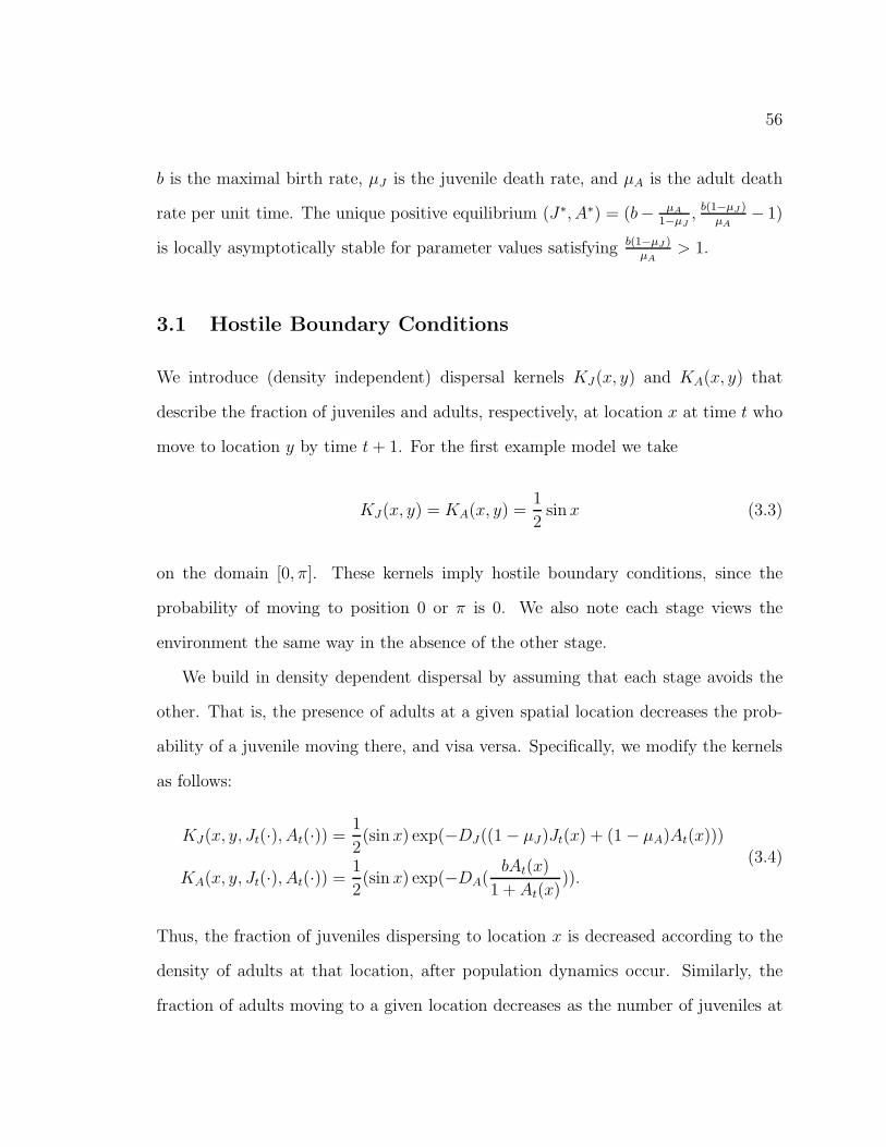
56
b is the maximal birth rate, µJ is the juvenile death rate, and µA is the adult death
rate per unit time. The unique positive equilibrium (J∗, A∗) = (b− µA
1−µJ, b(1−µJ )
µA− 1)
is locally asymptotically stable for parameter values satisfying b(1−µJ )µA
> 1.
3.1 Hostile Boundary Conditions
We introduce (density independent) dispersal kernels KJ(x, y) and KA(x, y) that
describe the fraction of juveniles and adults, respectively, at location x at time t who
move to location y by time t + 1. For the first example model we take
KJ(x, y) = KA(x, y) =1
2sin x (3.3)
on the domain [0, π]. These kernels imply hostile boundary conditions, since the
probability of moving to position 0 or π is 0. We also note each stage views the
environment the same way in the absence of the other stage.
We build in density dependent dispersal by assuming that each stage avoids the
other. That is, the presence of adults at a given spatial location decreases the prob-
ability of a juvenile moving there, and visa versa. Specifically, we modify the kernels
as follows:
KJ(x, y, Jt(·), At(·)) =1
2(sin x) exp(−DJ((1 − µJ)Jt(x) + (1 − µA)At(x)))
KA(x, y, Jt(·), At(·)) =1
2(sin x) exp(−DA(
bAt(x)
1 + At(x))).
(3.4)
Thus, the fraction of juveniles dispersing to location x is decreased according to the
density of adults at that location, after population dynamics occur. Similarly, the
fraction of adults moving to a given location decreases as the number of juveniles at
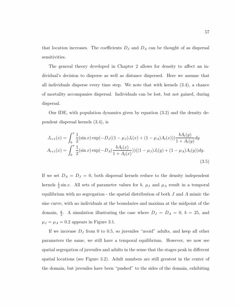
57
that location increases. The coefficients DJ and DA can be thought of as dispersal
sensitivities.
The general theory developed in Chapter 2 allows for density to affect an in-
dividual’s decision to disperse as well as distance dispersed. Here we assume that
all individuals disperse every time step. We note that with kernels (3.4), a chance
of mortality accompanies dispersal. Individuals can be lost, but not gained, during
dispersal.
Our IDE, with population dynamics given by equation (3.2) and the density de-
pendent dispersal kernels (3.4), is
Jt+1(x) =
∫ π
0
1
2(sin x) exp(−DJ((1 − µJ)Jt(x) + (1 − µA)At(x)))
bAt(y)
1 + At(y)dy
At+1(x) =
∫ π
0
1
2(sin x) exp(−DA(
bAt(x)
1 + At(x)))((1 − µJ)Jt(y) + (1 − µA)At(y))dy.
(3.5)
If we set DA = DJ = 0, both dispersal kernels reduce to the density independent
kernels 12sin x. All sets of parameter values for b, µJ and µA result in a temporal
equilibrium with no segregation - the spatial distribution of both J and A mimic the
sine curve, with no individuals at the boundaries and maxima at the midpoint of the
domain, π2. A simulation illustrating the case where DJ = DA = 0, b = 25, and
µJ = µA = 0.2 appears in Figure 3.1.
If we increase DJ from 0 to 0.5, so juveniles “avoid” adults, and keep all other
parameters the same, we still have a temporal equilibrium. However, we now see
spatial segregation of juveniles and adults in the sense that the stages peak in different
spatial locations (see Figure 3.2). Adult numbers are still greatest in the center of
the domain, but juveniles have been “pushed” to the sides of the domain, exhibiting
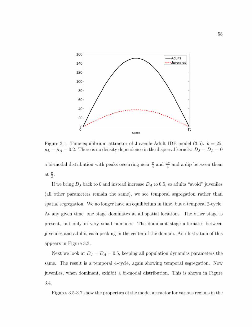
58
0 0
20
40
60
80
100
120
140
160
Space
AdultsJuveniles
π
Figure 3.1: Time-equilibrium attractor of Juvenile-Adult IDE model (3.5). b = 25,µL = µA = 0.2. There is no density dependence in the dispersal kernels: DJ = DA = 0
a bi-modal distribution with peaks occurring near π4
and 3π4
and a dip between them
at π2.
If we bring DJ back to 0 and instead increase DA to 0.5, so adults “avoid” juveniles
(all other parameters remain the same), we see temporal segregation rather than
spatial segregation. We no longer have an equilibrium in time, but a temporal 2-cycle.
At any given time, one stage dominates at all spatial locations. The other stage is
present, but only in very small numbers. The dominant stage alternates between
juveniles and adults, each peaking in the center of the domain. An illustration of this
appears in Figure 3.3.
Next we look at DJ = DA = 0.5, keeping all population dynamics parameters the
same. The result is a temporal 4-cycle, again showing temporal segregation. Now
juveniles, when dominant, exhibit a bi-modal distribution. This is shown in Figure
3.4.
Figures 3.5-3.7 show the properties of the model attractor for various regions in the
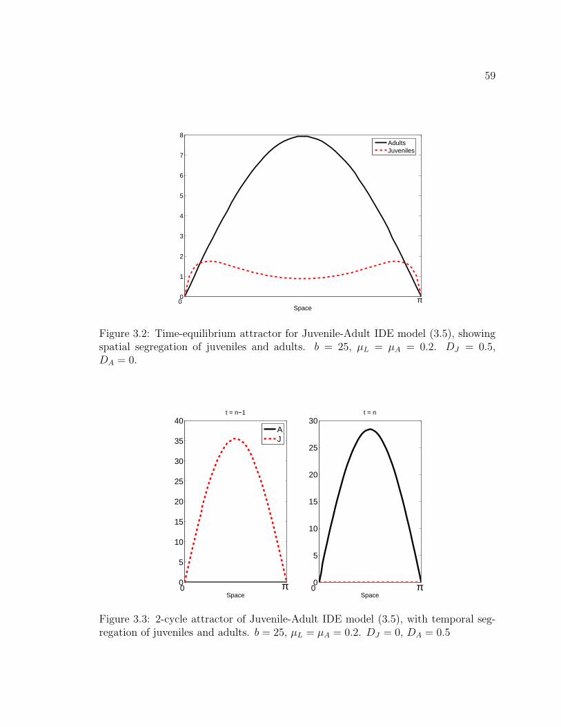
59
0 0
1
2
3
4
5
6
7
8
Space
AdultsJuveniles
π
Figure 3.2: Time-equilibrium attractor for Juvenile-Adult IDE model (3.5), showingspatial segregation of juveniles and adults. b = 25, µL = µA = 0.2. DJ = 0.5,DA = 0.
0 0
5
10
15
20
25
30
35
40
Space
t = n−1
0 0
5
10
15
20
25
30
Space
t = n
AJ
π π
Figure 3.3: 2-cycle attractor of Juvenile-Adult IDE model (3.5), with temporal seg-regation of juveniles and adults. b = 25, µL = µA = 0.2. DJ = 0, DA = 0.5
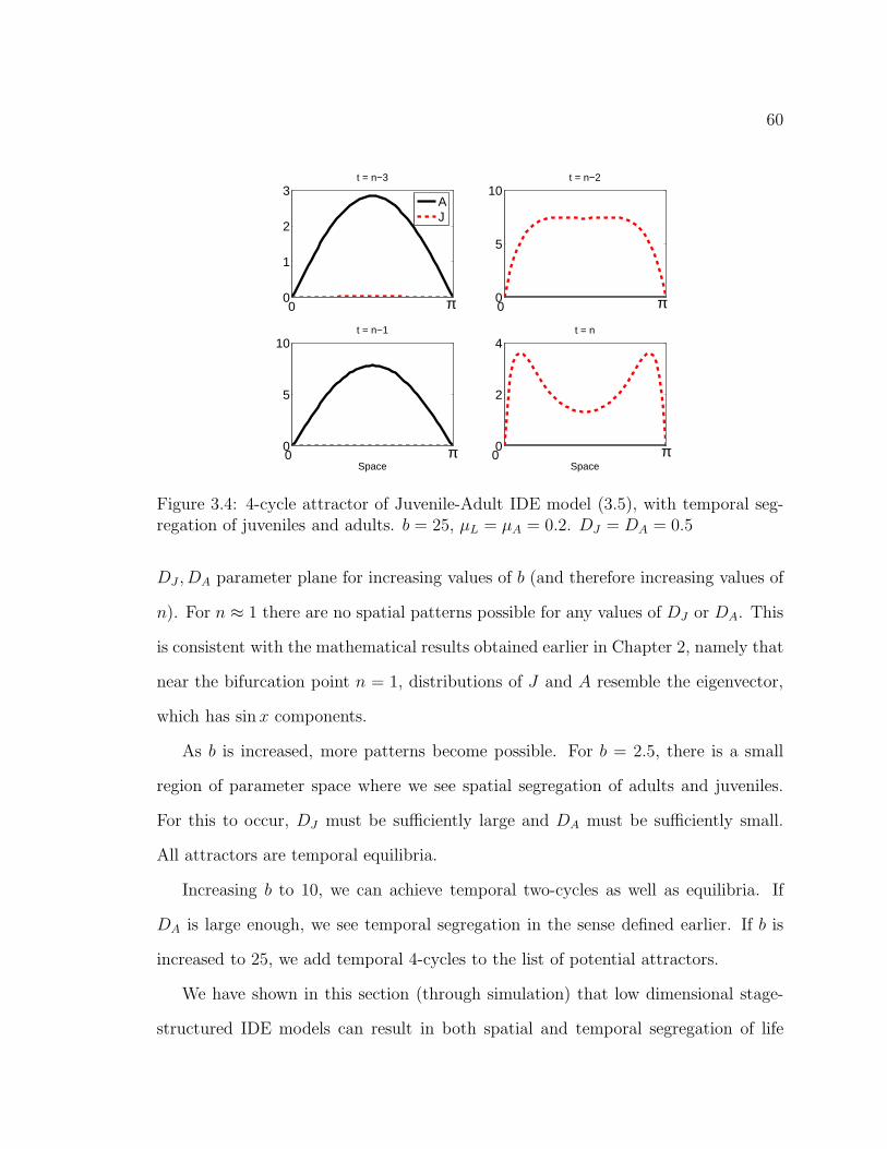
60
00
1
2
3t = n−3
0 0
5
10t = n−2
0 0
5
10
Space
t = n−1
0 0
2
4
Space
t = n
AJ
π
π
π
π
Figure 3.4: 4-cycle attractor of Juvenile-Adult IDE model (3.5), with temporal seg-regation of juveniles and adults. b = 25, µL = µA = 0.2. DJ = DA = 0.5
DJ , DA parameter plane for increasing values of b (and therefore increasing values of
n). For n ≈ 1 there are no spatial patterns possible for any values of DJ or DA. This
is consistent with the mathematical results obtained earlier in Chapter 2, namely that
near the bifurcation point n = 1, distributions of J and A resemble the eigenvector,
which has sin x components.
As b is increased, more patterns become possible. For b = 2.5, there is a small
region of parameter space where we see spatial segregation of adults and juveniles.
For this to occur, DJ must be sufficiently large and DA must be sufficiently small.
All attractors are temporal equilibria.
Increasing b to 10, we can achieve temporal two-cycles as well as equilibria. If
DA is large enough, we see temporal segregation in the sense defined earlier. If b is
increased to 25, we add temporal 4-cycles to the list of potential attractors.
We have shown in this section (through simulation) that low dimensional stage-
structured IDE models can result in both spatial and temporal segregation of life

61
Figure 3.5: Shown is a section of the DJ − DA parameter plane for b = 2.5. µJ =µA = 0.2. We look at 0 ≤ DJ ≤ 1 and 0 ≤ DA ≤ 1. All combinations of DJ and DA
in this range result in equilibrium dynamics for model (3.5). Spatial segregation ispossible for large enough DJ and small enough DA.
Figure 3.6: Shown is a section of the DJ − DA parameter plane for b = 10. µJ =µA = 0.2. In addition to the model (3.5) attractors seen for b = 2.5, we can also see2 − cycles and temporal segregation.
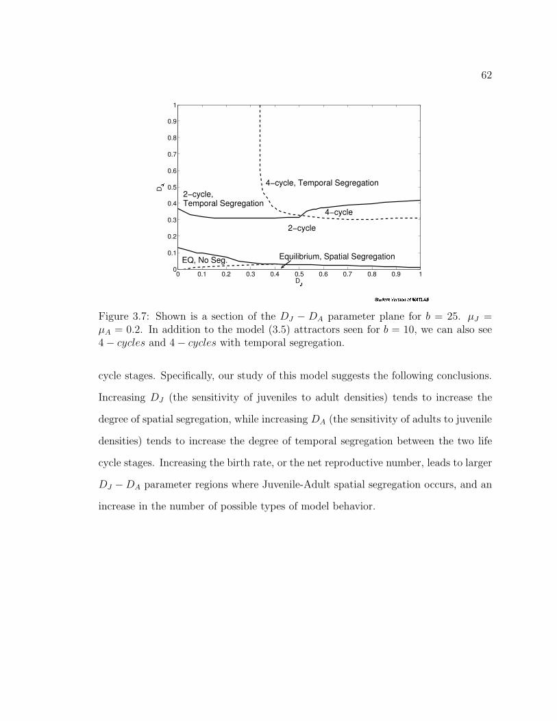
62
Figure 3.7: Shown is a section of the DJ − DA parameter plane for b = 25. µJ =µA = 0.2. In addition to the model (3.5) attractors seen for b = 10, we can also see4 − cycles and 4 − cycles with temporal segregation.
cycle stages. Specifically, our study of this model suggests the following conclusions.
Increasing DJ (the sensitivity of juveniles to adult densities) tends to increase the
degree of spatial segregation, while increasing DA (the sensitivity of adults to juvenile
densities) tends to increase the degree of temporal segregation between the two life
cycle stages. Increasing the birth rate, or the net reproductive number, leads to larger
DJ − DA parameter regions where Juvenile-Adult spatial segregation occurs, and an
increase in the number of possible types of model behavior.

63
3.1.1 Application of Theory
Here we apply the theory developed in Chapter 2 to the Juvenile-Adult IDE model
(3.5). We let ~x(t, s) = (Jt(s), At(s)). Then
T (s, v, ~x(t, ·)) =
0 0
(1 − µJ) sin s2
exp(−DAJJt(s)) (1 − µA) sin s2
exp(−DAJJt(s))
(3.6)
and
F (s, v, ~x(t, ·)) =
0 b1+At(v)
sin s2
exp(−DJAAt(s))
0 0
. (3.7)
T (s, v,~0) =
0 0
(1 − µJ) sin s2
(1 − µA) sin s2
(3.8)
and
F (s, v,~0) =
0 b sin s2
0 0
(3.9)
so the operators T and F are the same as in Example 2.4.2 with s1 = (1 − µJ) and
s2 = (1 − µA).
The resolvent of T is the same as for Example 2.4.2 (equation (2.33)). The operator
(I − T )−1F is
(I − T )−1F :
J(s)
A(s)
→
b sin s2
∫ π
0A(v)dv
sin s2
(1−µJ )µA
∫ π
0b sin v
2
∫ π
0A(σ)dσdv
(3.10)
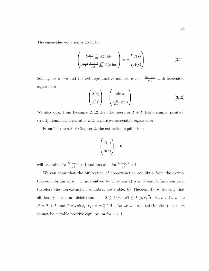
64
The eigenvalue equation is given by
b sin s2
∫ π
0A(v)dv
b sin s2
(1−µJ )µA
∫ π
0A(σ)dσ
= n
J(s)
A(s)
(3.11)
Solving for n, we find the net reproductive number is n = b(1−µJ )µA
with associated
eigenvector
J(s)
A(s)
=
sin s
1−µJ
µAsin s
. (3.12)
We also know from Example 2.4.2 that the operator T + F has a simple, positive,
strictly dominant eigenvalue with a positive associated eigenvector.
From Theorem 3 of Chapter 2, the extinction equilibrium
J(s)
A(s)
= ~0
will be stable for b(1−µJ )µA
< 1 and unstable for b(1−µJ )µA
> 1.
We can show that the bifurcation of non-extinction equilibria from the extinc-
tion equilibrium at n = 1 (guaranteed by Theorem 2) is a forward bifurcation (and
therefore the non-extinction equilibria are stable, by Theorem 4) by showing that
all density effects are deleterious, i.e. 0 ≤ P (s, v, ~x) ≤ P (s, v,~0) ∀s, v ∈ Ω, where
P = T + F and ~x = col(x1, x2) = col(J, A). As we will see, this implies that there
cannot be a stable positive equilibrium for n < 1.
65
For our model,
P (s, v, ~x(t, ·)) =
0 b1+x2(t,v)
sin s2
exp(−D12x2(t, s))
(1 − µ1)sin s2
exp(−DAJJt(s)) (1 − µ2)sin s
2exp(−D21x1(t, s))
(3.13)
where D12 = DJA, D21 = DAJ , µ1 = µJ and µ2 = µA.
P (s, v,~0) =
0 b sin s2
(1 − µ1)sin s
2(1 − µ2)
sin s2
(3.14)
Since 11+x2(t,v)
≤ 1, exp(−D12x2(t, s)) ≤ 1 and exp(−D21x1(t, s)) ≤ 1, it follows
that
0 ≤ P (s, v, ~x(t, ·)) ≤ P (s, v,~0) ∀s, v ∈ Ω.
Let
~y(t + 1, s) =
∫
Ω
0 b sin s2
(1 − µJ) sin s2
(1 − µA) sin s2
~y(t, v)dv, ~y(0, s) = ~x(0, s). (3.15)
Assume ~x(t, s) ≤ ~y(t, s) ∀s ∈ Ω. Then
~x(t + 1, s) =
b sin s2
e−D12x2(s)∫
Ωx2(t,v)
1+x2(t,v)dv
sin s2
e−D21x1(s)∫
Ω(1 − µ1)x1(v) + (1 − µ2)x2(v)dv
≤
b sin s2
∫
Ωy2(t, v)dv
sin s2
∫
Ω(1 − µ1)x1(v) + (1 − µ2)x2(v)dv
= ~y(t + 1, s)
(3.16)
By induction,
~x(t + 1, s) ≤ ~y(t + 1, s) ∀s ∈ Ω, ∀t (3.17)
66
and
|y| → 0 ⇒ |x| → 0. (3.18)
Let λ0 denote the dominant eigenvalue of P (s, v,~0). By Theorem 6, if n < 1 then
λ0 < 1 and |y| → 0 as t → ∞. Thus the extinction equilibrium ~x = ~0 is a global
attractor for n < 1 and the bifurcation cannot be to the left. This result is shown by
Cushing [6] for non-spatial models.
The equilibria of model (3.5) can be approximated by the eigenvector (3.12) for
values of n near 1. Since both components of the eigenvector are multiples of sin s,
there is no spatial segregation of juveniles and adults for n ≈ 1. Figures 3.5-3.7 show
the spatial patterns for model attractors in a region of DJ , DA parameter space for
n = 10,n = 40, and n = 100. The smallest n shown, n = 10 gives rise to spatial
segregation of juveniles and adults in a small region of parameter space. For n ≈ 1,
the only attractor seen is a temporal equilibrium with no spatial segregation. As
n increases, we found, however, that the effects of density dependence can cause
segregation of life cycle stages to occur.
3.2 Mixed Boundary Conditions
The spatial pattern observed by Arthur Ghent in T. castaneum [14] in a cylindrical
vial of flour can be looked at as one-dimensional in space, where the spatial dimension
is depth. Due to gravity, there is a gradient of increasing flour density from the surface
to bottom of the bottle [14]. Individuals can live on the surface but cannot pass above
it. We model this environment as a one-dimensional domain with mixed boundary
conditions, where the bottom of the bottle is a hostile boundary and the surface is a
no-flux boundary.
67
We are interested in the behavior of a Juvenile-Adult IDE model with these bound-
ary conditions. Ghent’s study was done with an organism best modeled with three
life-stages, but here we investigate what qualitative aspects of his observations can
be captured by a two life-stage model.
For this Juvenile-Adult IDE model with mixed boundary conditions, we use the
population dynamics model (3.2) and again build our boundary conditions into the
kernel. The kernels we use are
KJ(x, Jt(x), At(x)) = exp(−DJ ((1 − µJ)Jt(x) + (1 − µA)At(x))) cos x
KA(x, Jt(x), At(x)) = exp(−DA(bAt(x)
1 + At(x))) cosx.
(3.19)
Here KJ gives the fraction of juveniles at position y at time t who move to posi-
tion x by time t + 1. The spatial domain is the interval [0, π2]. The left endpoint,
0 (representing the surface of the bottle), is the no-flux boundary. The right end-
point, π2
(representing the bottom of the bottle), is the hostile boundary. Again this
kernel assumes that juveniles avoid adults and adults avoid juveniles. The juvenile-
adult integrodifference equation model (3.5) with these mixed boundary conditions
becomes:
Jt+1(x) =
∫ π2
0
1
2exp(−DJ((1 − µJ)Jt(x) + (1 − µA)At(x)))(cos x)
bAt(y)
1 + At(y)dy
At+1(x) =
∫ π2
0
1
2exp(−DA(
bAt(x)
1 + At(x)))(cos x)((1 − µJ)Jt(y) + (1 − µA)At(y))dy
(3.20)
Matlab simulations of model (3.20) for reasonable parameters for Tribolium show
model dynamics qualitatively similar to behavior observed by Ghent. For example
the simulation shown in Figure 3.8 shows juveniles moving to avoid high densities
68
of adults, and adult movement uninfluenced by the presence of juveniles. Adult
densities peak near the surface, and juveniles peak below the surface (closer to the
bottom of the bottle). While we don’t expect to be able to compare, accurately
or quantitatively, observations from Tribolium cultures with simulations from simple
Juvenile-Adult toy models, we note that lower dimensional IDE models with density
dependent dispersal can give rise to patterns qualitatively similar to those observed
in Tribolium. In Chapter 4 we will investigate a spatial extension of the biologically
more accurate three-dimensional LPA model and study what spatial patterns are
possible in that model.
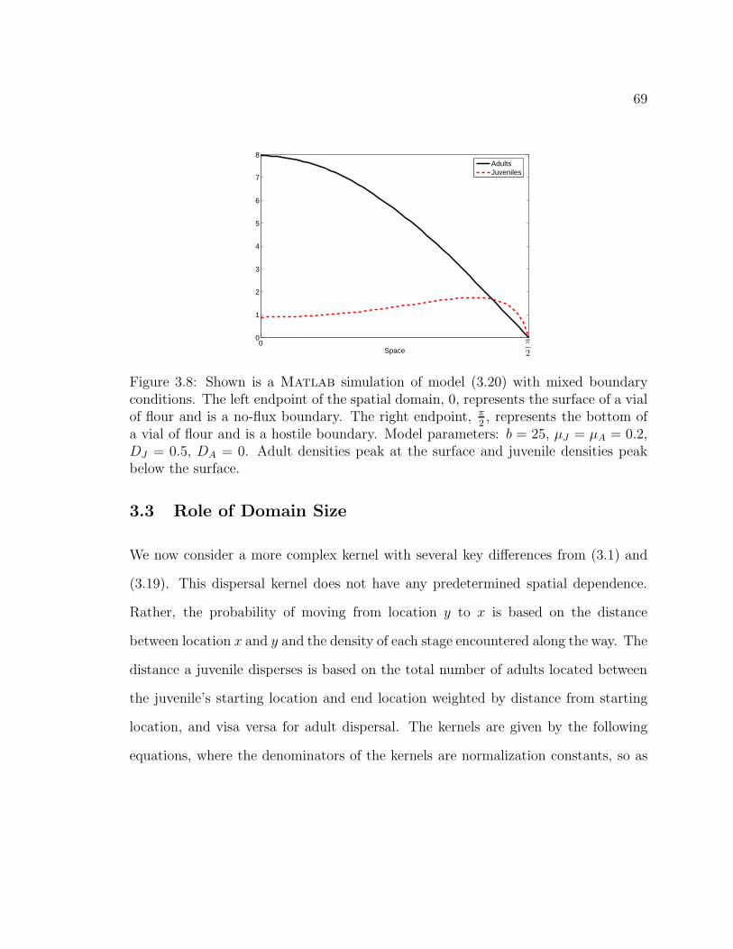
69
0 0
1
2
3
4
5
6
7
8
Space
AdultsJuveniles
π
2
Figure 3.8: Shown is a Matlab simulation of model (3.20) with mixed boundaryconditions. The left endpoint of the spatial domain, 0, represents the surface of a vialof flour and is a no-flux boundary. The right endpoint, π
2, represents the bottom of
a vial of flour and is a hostile boundary. Model parameters: b = 25, µJ = µA = 0.2,DJ = 0.5, DA = 0. Adult densities peak at the surface and juvenile densities peakbelow the surface.
3.3 Role of Domain Size
We now consider a more complex kernel with several key differences from (3.1) and
(3.19). This dispersal kernel does not have any predetermined spatial dependence.
Rather, the probability of moving from location y to x is based on the distance
between location x and y and the density of each stage encountered along the way. The
distance a juvenile disperses is based on the total number of adults located between
the juvenile’s starting location and end location weighted by distance from starting
location, and visa versa for adult dispersal. The kernels are given by the following
equations, where the denominators of the kernels are normalization constants, so as
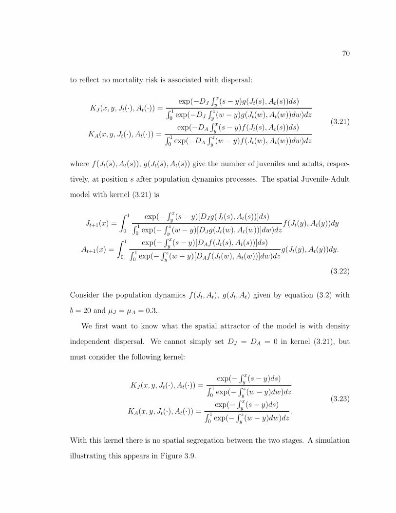
70
to reflect no mortality risk is associated with dispersal:
KJ(x, y, Jt(·), At(·)) =exp(−DJ
∫ x
y(s − y)g(Jt(s), At(s))ds)
∫ 1
0exp(−DJ
∫ z
y(w − y)g(Jt(w), At(w))dw)dz
KA(x, y, Jt(·), At(·)) =exp(−DA
∫ x
y(s − y)f(Jt(s), At(s))ds)
∫ 1
0exp(−DA
∫ z
y(w − y)f(Jt(w), At(w))dw)dz
(3.21)
where f(Jt(s), At(s)), g(Jt(s), At(s)) give the number of juveniles and adults, respec-
tively, at position s after population dynamics processes. The spatial Juvenile-Adult
model with kernel (3.21) is
Jt+1(x) =
∫ 1
0
exp(−∫ x
y(s − y)[DJg(Jt(s), At(s))]ds)
∫ 1
0exp(−
∫ z
y(w − y)[DJg(Jt(w), At(w))]dw)dz
f(Jt(y), At(y))dy
At+1(x) =
∫ 1
0
exp(−∫ x
y(s − y)[DAf(Jt(s), At(s))]ds)
∫ 1
0exp(−
∫ z
y(w − y)[DAf(Jt(w), At(w))]dw)dz
g(Jt(y), At(y))dy.
(3.22)
Consider the population dynamics f(Jt, At), g(Jt, At) given by equation (3.2) with
b = 20 and µJ = µA = 0.3.
We first want to know what the spatial attractor of the model is with density
independent dispersal. We cannot simply set DJ = DA = 0 in kernel (3.21), but
must consider the following kernel:
KJ(x, y, Jt(·), At(·)) =exp(−
∫ x
y(s − y)ds)
∫ 1
0exp(−
∫ z
y(w − y)dw)dz
KA(x, y, Jt(·), At(·)) =exp(−
∫ x
y(s − y)ds)
∫ 1
0exp(−
∫ z
y(w − y)dw)dz
.
(3.23)
With this kernel there is no spatial segregation between the two stages. A simulation
illustrating this appears in Figure 3.9.
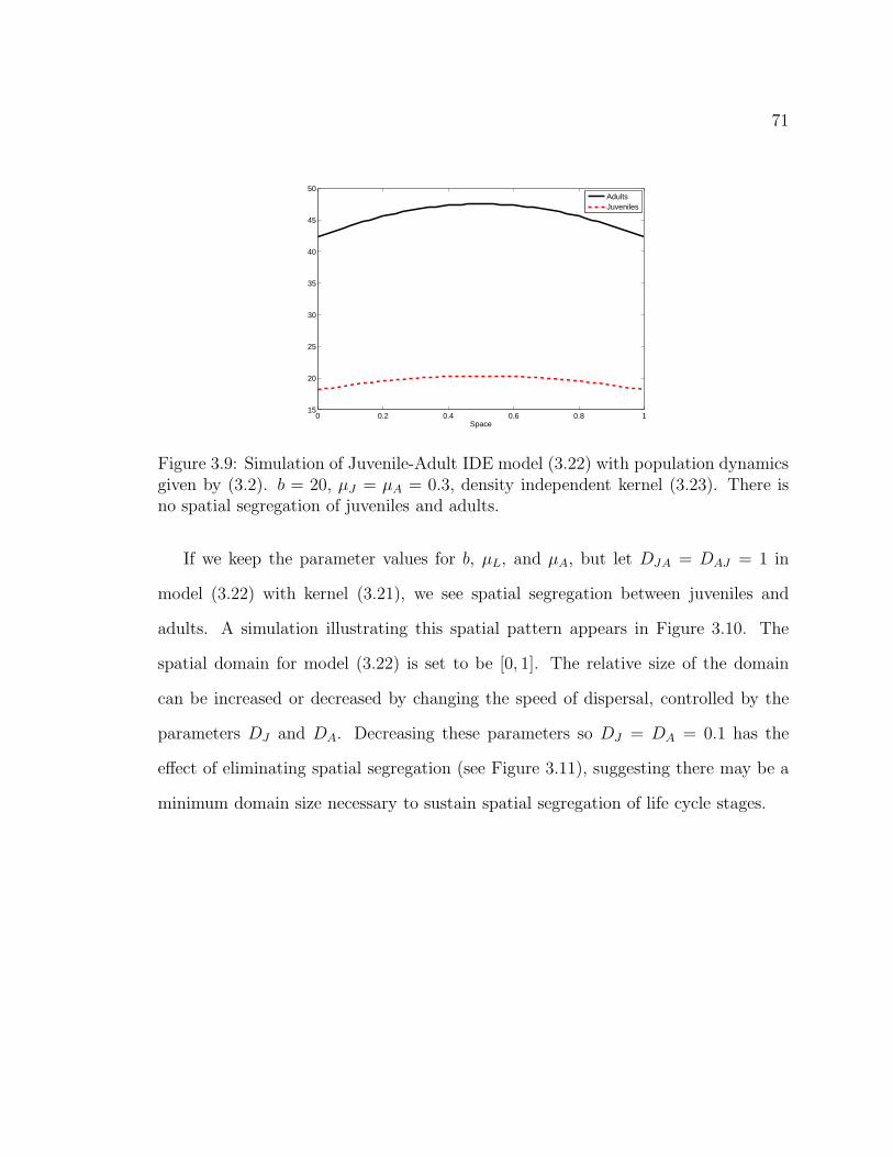
71
0 0.2 0.4 0.6 0.8 115
20
25
30
35
40
45
50
Space
AdultsJuveniles
Figure 3.9: Simulation of Juvenile-Adult IDE model (3.22) with population dynamicsgiven by (3.2). b = 20, µJ = µA = 0.3, density independent kernel (3.23). There isno spatial segregation of juveniles and adults.
If we keep the parameter values for b, µL, and µA, but let DJA = DAJ = 1 in
model (3.22) with kernel (3.21), we see spatial segregation between juveniles and
adults. A simulation illustrating this spatial pattern appears in Figure 3.10. The
spatial domain for model (3.22) is set to be [0, 1]. The relative size of the domain
can be increased or decreased by changing the speed of dispersal, controlled by the
parameters DJ and DA. Decreasing these parameters so DJ = DA = 0.1 has the
effect of eliminating spatial segregation (see Figure 3.11), suggesting there may be a
minimum domain size necessary to sustain spatial segregation of life cycle stages.
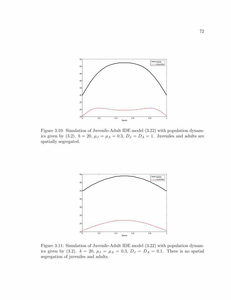
72
0 0.2 0.4 0.6 0.8 115
20
25
30
35
40
45
50
55
Space
AdultsJuveniles
Figure 3.10: Simulation of Juvenile-Adult IDE model (3.22) with population dynam-ics given by (3.2). b = 20, µJ = µA = 0.3, DJ = DA = 1. Juveniles and adults arespatially segregated.
0 0.2 0.4 0.6 0.8 115
20
25
30
35
40
45
50
Space
AdultsJuveniles
Figure 3.11: Simulation of Juvenile-Adult IDE model (3.22) with population dynam-ics given by (3.2). b = 20, µJ = µA = 0.3, DJ = DA = 0.1. There is no spatialsegregation of juveniles and adults.

73
Chapter 4
Case Studies Using Models for Flour Beetles
(Tribolium)
4.1 Spatial Patterns in Tribolium castaneum
4.1.1 The LPA Model
As discussed in Chapter 1, one of the most heavily analyzed and well-validated mod-
els in mathematical ecology is the “Larva-Pupa-Adult” (LPA) model, a three dimen-
sional system of nonlinear difference equations designed to describe the population
dynamics of Tribolium castaneum and Tribolium confusum [5]:
Lt+1 = bA(t)e−celL(t)−ceaA(t)
Pt+1 = (1 − µL)L(t)
At+1 = Pte−cpaAt + (1 − µA)At
(4.1)
L(t) represents the number of larvae at time t, P (t) gives the number of individuals
in the “P stage” (which includes non-feeding larvae, pupae, and callow adults) at
time t, and A(t) gives the number of sexually mature adults at time t. Animals
transit to the next class in two weeks, and we use this as the time step for the model.
Upon reaching the adult class, animals remain there until death. Larval recruitment
in the absence of egg cannibalism occurs at an inherent rate b. Eggs must survive
74
cannibalism by larvae and adults in order to become larvae, and the exponential
exp(−celL(t) − ceaA(t)) represents the survival per unit time. cel ≥ 0 and cea ≥ 0
are cannibalism coefficients of eggs by larvae and eggs by adults, respectively. It
is assumed that cannibalism occurs as a result of random encounters of larvae and
adults with eggs, which accounts for the exponential nonlinearities used [7]. Larvae
die at a rate µL, 0 < µL < 1, and so a fraction (1 − µL) survive to become pupae.
The natural death rate of pupae is negligible, so there is no µP term included in the
model. Pupae must escape cannibalism by adults (cpa) to become adults. Adults die
at a rate µA, 0 < µA < 1, and so at each census, the fraction of surviving adults is
(1 − µA).
4.1.2 The Spatial LPA Model
Our goal in this section is to construct a spatial extension of the LPA model in
order to explain the spatial patterns in T. castaneum and T. confusum observed by
Ghent [14] and detailed in Chapter 1. In order to construct the spatial LPA model,
we need to make assumptions regarding the dispersal behavior of the two mobile
life-stages, larvae and adults (pupae are immobile). We assume adults prefer areas
with lower larval densities than their current location and larvae prefer areas with
lower adult densities than their current location. Thus the fraction of large larvae
that move from location y to location x depends on the difference in adult densities,
after population dynamics occur, between the two locations. Adult dispersal depends
similarly on density of large larvae. We take our spatial domain Ω to be the finite
interval [0, π2] representing depth in a cylindrical vial, with 0 corresponding to the
surface of a cylindrical and 1 corresponding to the bottom of the vial. We assume
both larvae and adults view the environment in the same way, preferring flour near

75
the surface over the more dense flour near the bottom, as described earlier in section
3.2. We model this with mixed boundary conditions, assuming a no-flux boundary at
the surface and a hostile boundary at the bottom. The kernels for larval and adult
spatial redistribution are given by the following, respectively:
KL =1
C1
e−DLA(e−cpaAt(x)Pt(x)+(1−µA)At(x))−(e−cpaAt(y)Pt(y)+(1−µA)At(y))(cosm x)
KA =1
C2
e−DAL(bAt(x)e−ceaAt(x)−celLt(x))−(bAt(y)e−ceaAt(y)−celLt(y))(cosm x)
(4.2)
where C1 and C2 are the following normalization constants:
C1 =
∫ π2
0
e−DLA(e−cpaAt(x′)Pt(x′)+(1−µA)At(x′))−(e−cpaAt(y)Pt(y)+(1−µA)At(y))(cosm x′)dx′
C2 =
∫ π2
0
e−DAL(bAt(x′)e−ceaAt(x′)−celLt(x
′))−(bAt(y)e−ceaAt(y)−celLt(y))(cosm x′)dx′
(4.3)
The term cosm x in the dispersal kernel incorporates density independent spatial
preference. As the parameter m increases, the undesirable region at the bottom
of the bottle grows in size.
After simplification, the spatial LPA model becomes
Lt+1(x) =
∫ π2
0
1
c1
e−DLA(e−cpaAt(x)Pt(x)+(1−µA)At(x))(cosm x)(bAt(y)e−celLt(y)−ceaAt(y))dy
Pt+1(x) =(1 − µL)Lt(x)
At+1(x) =
∫ π2
0
1
c2e−DAL(bAt(x)e−ceaAt(x)−celLt(x))(cosm x)(e−cpaAt(y)Pt(y)
+ (1 − µA)At(y))dy
(4.4)
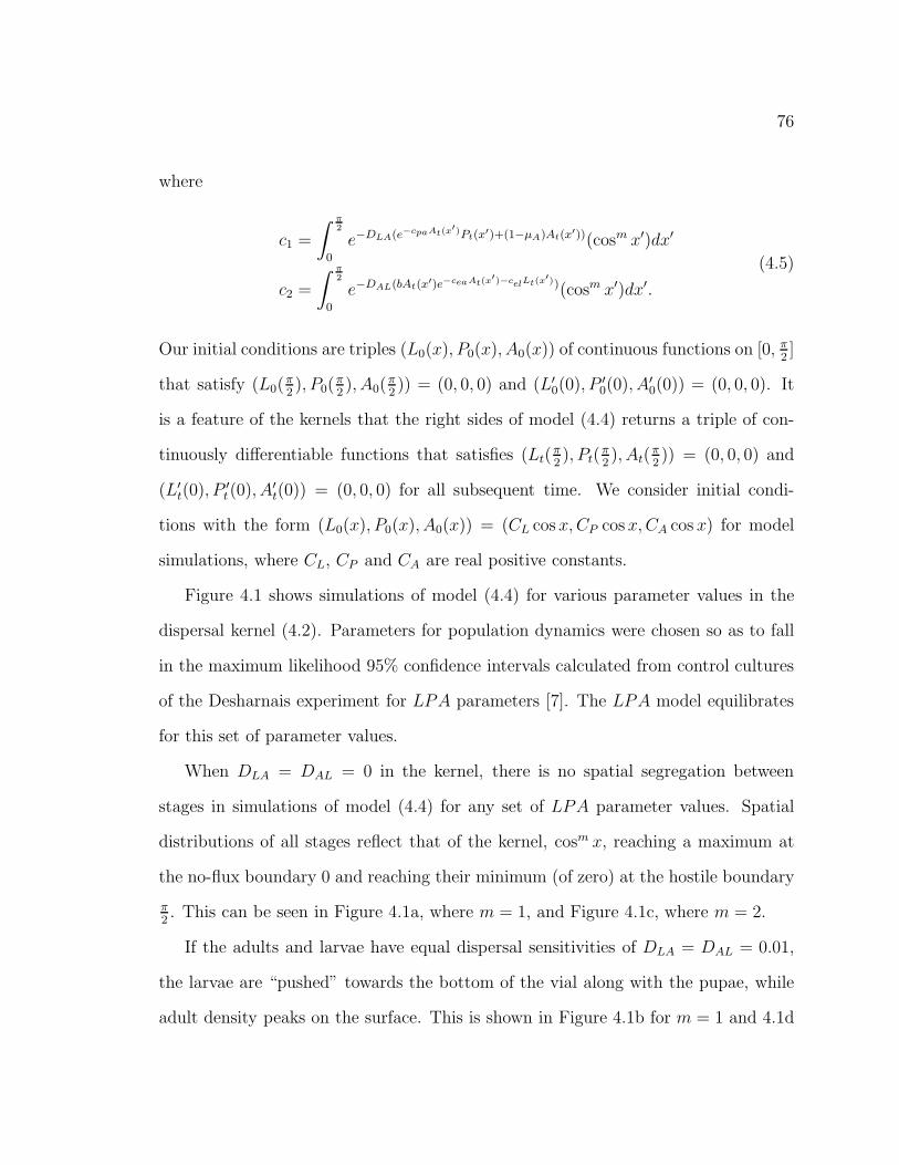
76
where
c1 =
∫ π2
0
e−DLA(e−cpaAt(x′)Pt(x′)+(1−µA)At(x′))(cosm x′)dx′
c2 =
∫ π2
0
e−DAL(bAt(x′)e−ceaAt(x′)−celLt(x
′))(cosm x′)dx′.
(4.5)
Our initial conditions are triples (L0(x), P0(x), A0(x)) of continuous functions on [0, π2]
that satisfy (L0(π2), P0(
π2), A0(
π2)) = (0, 0, 0) and (L′
0(0), P ′0(0), A′
0(0)) = (0, 0, 0). It
is a feature of the kernels that the right sides of model (4.4) returns a triple of con-
tinuously differentiable functions that satisfies (Lt(π2), Pt(
π2), At(
π2)) = (0, 0, 0) and
(L′t(0), P ′
t(0), A′t(0)) = (0, 0, 0) for all subsequent time. We consider initial condi-
tions with the form (L0(x), P0(x), A0(x)) = (CL cos x, CP cos x, CA cos x) for model
simulations, where CL, CP and CA are real positive constants.
Figure 4.1 shows simulations of model (4.4) for various parameter values in the
dispersal kernel (4.2). Parameters for population dynamics were chosen so as to fall
in the maximum likelihood 95% confidence intervals calculated from control cultures
of the Desharnais experiment for LPA parameters [7]. The LPA model equilibrates
for this set of parameter values.
When DLA = DAL = 0 in the kernel, there is no spatial segregation between
stages in simulations of model (4.4) for any set of LPA parameter values. Spatial
distributions of all stages reflect that of the kernel, cosm x, reaching a maximum at
the no-flux boundary 0 and reaching their minimum (of zero) at the hostile boundary
π2. This can be seen in Figure 4.1a, where m = 1, and Figure 4.1c, where m = 2.
If the adults and larvae have equal dispersal sensitivities of DLA = DAL = 0.01,
the larvae are “pushed” towards the bottom of the vial along with the pupae, while
adult density peaks on the surface. This is shown in Figure 4.1b for m = 1 and 4.1d

77
for m = 2. Both of these results are qualitatively similar to Ghent’s observations
shown in Figure 1.1. As the parameter m is increased, the bottom of the habitat
becomes increasingly undesirable to both stages. The adults reach their maximum
density at the surface for all values of m, but the peak of the larval distribution moves
towards the surface as m increases.
00
20
40
60
80
100
120
140
160
Space
LarvaePupaeAdults
π
2
(a) m = 1, DLA = DAL = 0
00
50
100
150
200
250
Space
LarvaePupaeAdults
π
2
(b) m = 1, DLA = DAL = 0.01
00
20
40
60
80
100
120
140
160
180
Space
LarvaePupaeAdults
π
2
(c) m = 2, DLA = DAL = 0
00
50
100
150
200
250
300
350
Space
LarvaePupaeAdults
π
2
(d) m = 2, DLA = DAL = 0.01
Figure 4.1: Simulations of the spatial LPA model (4.4) for various parameter valuesin the dispersal kernels (4.2). All attractors shown are temporal equilibria. LPAparameter values given by: b = 10, cel = 0.01, cea = 0.0175, µL = 0.435, cpa = 0.016,µA = 0.075.
In general, spatial segregation of larvae and adults is observed for a range of
DLA > 0, even if DAL = 0. The effect is more severe when combined with values of
DAL > 0, but this is not necessary. However, the reverse is not true. It is necessary
that larvae move in response to adult densities; if DLA = 0 and only adults disperse in
78
response to larval densities, we do not see the segregation. Adults will not be pushed
to the bottom of the habitat for any values of DLA and DAL. Furthermore, if DLA
and/or DAL become too large, we begin to see temporal patterns as well.
We did not observe multiple attractors of the spatial LPA model for the range
of parameter values considered. Initial conditions of the form (L0(x), P0(x), A0(x))
= (CL cosm x, CP cosm x, CA cosm x), where CL, CP , CA and m are real positive con-
stants lead to the attractors in Figure 4.1. The boundary conditions can also be
satisfied by piecewise continuous step functions of the form (L0(x), P0(x), A0(x)) =
(CLIx<x∗, CP Ix<x∗, CAIx<x∗), where CL, CP , CA are real positive constants and Ix<x∗
is equal to 1 on 0 ≤ x ≤ x∗ and 0 on x∗ ≤ x ≤ π2. This set of initial conditions also
leads to the attractors in Figure 4.1.
4.2 Spatial Patterns in Tribolium brevicornis
As pointed out in Chapter 1, the flour beetle Tribolium brevicornis has major biolog-
ical differences from Tribolium castaneum that prevent the LPA model from being
used to describe its population dynamics accurately. The most glaring difference is
that T. brevicornis is an inhibitor. In the presence of high adult densities, larvae of
this species may fail to pupate. Whereas T. castaneum larvae always pupate after
spending two weeks as a larva, T. brevicornis larvae may remain in the larval stage
indefinitely. When local adult densities lower, T. brevicornis larvae will go on to pu-
pate. Secondly, the innate length of the larval stage for T. brevicornis in the absence
of adults is four weeks (rather than the two weeks for T. castaneum). During the
second two-week interval, larvae are noticeably larger and more mobile than in their
first two-weeks as small larvae. A third biological difference between these species is
79
the notable absence of pupal cannibalism by adults in T. brevicornis. Pupal canni-
balism is a mechanism that controls adult recruitment in other flour beetle species
such as T. castaneum and T. confusum, but T. brevicornis have the alternate control
mechanism of inhibition.
A question of considerable interest is that of the evolutionary or selective advan-
tage of inhibition. It is usually considered advantageous for a species to have high
numbers of reproductive adults, yet often laboratory cultures of T. brevicornis have
a larval population greater than the adult population. One can ask if being an in-
hibitor provides some kind of adaptive advantage for T. brevicornis. Of course, there
are many ways to define an advantage. We will look at one based on total population
size and the total numbers of animals in each class at equilibrium.
In order to model the spatial dynamics observed in T. brevicornis, we need a
non-spatial model to describe the population dynamics of the species. We modify
the LPA model to take into account the three main biological differences between T.
brevicornis and T. castaneum/T. confusum. We will refer to this new model as the
“SLPA′′ model.
4.2.1 The SLPA Model
In order to account for the longer larval stage, we split the “L” class of the LPA
model into two new classes and denote them by “S” and “L”. S(t) represents the
number of younger or “small larvae” at time t and L(t) now represents the number
of “large larvae” at time t. This class includes third week larvae as well as larvae
who have been inhibited for an indefinite amount of time. The time step of the
model remains two weeks. We model inhibition with a Ricker type, or exponential,
nonlinearity. This is appropriate given the assumption that inhibition is a result of
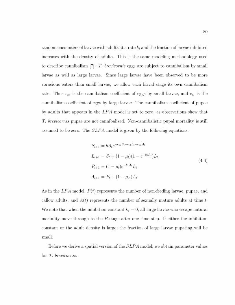
80
random encounters of larvae with adults at a rate ki and the fraction of larvae inhibited
increases with the density of adults. This is the same modeling methodology used
to describe cannibalism [7]. T. brevicornis eggs are subject to cannibalism by small
larvae as well as large larvae. Since large larvae have been observed to be more
voracious eaters than small larvae, we allow each larval stage its own cannibalism
rate. Thus ces is the cannibalism coefficient of eggs by small larvae, and cel is the
cannibalism coefficient of eggs by large larvae. The cannibalism coefficient of pupae
by adults that appears in the LPA model is set to zero, as observations show that
T. brevicornis pupae are not cannibalized. Non-cannibalistic pupal mortality is still
assumed to be zero. The SLPA model is given by the following equations:
St+1 = bAte−cesSt−celLt−ceaAt
Lt+1 = St + (1 − µl)(1 − e−kiAt)Lt
Pt+1 = (1 − µl)e−kiAtLt
At+1 = Pt + (1 − µA)At.
(4.6)
As in the LPA model, P (t) represents the number of non-feeding larvae, pupae, and
callow adults, and A(t) represents the number of sexually mature adults at time t.
We note that when the inhibition constant ki = 0, all large larvae who escape natural
mortality move through to the P stage after one time step. If either the inhibition
constant or the adult density is large, the fraction of large larvae pupating will be
small.
Before we derive a spatial version of the SLPA model, we obtain parameter values
for T. brevicornis.

81
4.2.2 Parametrization
Population data for T. brevicornis were collected by R. F. Costantino and R. A.
Desharnais in 1982 (R. F. Costantino, personal communication). Twenty adult beetles
were placed into a one-half pint bottle with 20 grams of medium (95% unbleached
wheat flour and 5% dried brewer’s yeast by weight). The beetles were incubated in
the dark at 33 ± 1 degree Celsius and 60 ± 5% relative humidity. Each such culture
was replicated four times.
Every two weeks the beetles were counted and the number of small larvae, large
larvae, pupae and adults were recorded in a vector (St, Lt, Pt, At). Eggs were not
counted. After the counting, live animals were placed back in the bottle with fresh
medium. Each culture was maintained for 36 weeks (18 time steps).
In order to connect the deterministic SLPA model with this data using the
methodology in [9, 11], we construct a stochastic version of the model. Given the
accuracy of the census counts, the two main types of noise to consider are envi-
ronmental and demographic. Environmental stochasticity is the result of external
changes to a system, whereas demographic stochasticity accounts for the variation
among individuals within the population in variables such as clutch size, probability
of dying, etc. Since the laboratory conditions are extremely well controlled, we con-
sider demographic noise to be more relevant to the conditions under which our data
were collected and will assume this type of noise when building our stochastic model.
(This was the case for T. castaneum in the extensive study of that species’ dynamics
in [6, 7].)
The stochastic SLPA model is constructed similarly to the stochastic LPA model
[9], namely, by taking advantage of the ability of binomial and poisson distributions

82
to model the aggregation of demographic events (such as birth and death) within
each life stage. Following the work of Dennis et al. [9], we can model the conditional
one-time-step distributions of St, Lt, Pt and At as independent, discrete distributions
of either Poisson, binomial or sums of Poisson and binomial random variables. For
each of these distributions, a square root transformation transforms the distribution
to one which is approximately normal with constant variance. We can then represent
our stochastic model as a nonlinear autoregressive (NLAR) model of the following
form [11]:
Wt = h(Wt−1) + Et (4.7)
where the distribution of Wt, given Wt−1, should be normally distributed with con-
stant variance σ2 that does not depend on wt−1, the state of the system at time
t − 1.
We propose the following stochastic version of the SLPA model for explaining
the observed time series data of T. brevicornis populations:
√
St+1 =√
bAte−cesSt−celLt−ceaAt + E1t
√
Lt+1 =√
St + (1 − µL)(1 − e−kiAt)Lt + E2t
√
Pt+1 =√
(1 − µL)e−kiAtLt + E3t
√
At+1 =√
Pt + (1 − µA)At + E4t
(4.8)
where Et = (E1t, E2t, E3t, E4t)′ is a random noise vector with a multivariate normal
distribution having mean (0, 0, 0, 0) and a diagonal variance-covariance matrix. We
denote the diagonal entries of this matrix by the vector Σ = (σ211, σ
222, σ
233, σ
244). The
assumed demographic nature of the noise implies that the off-diagonal covariances will
be equal to zero, and the Et will be uncorrelated through time [11]. The stochastic
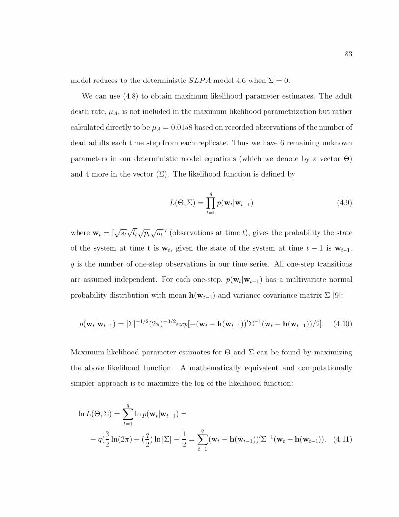
83
model reduces to the deterministic SLPA model 4.6 when Σ = 0.
We can use (4.8) to obtain maximum likelihood parameter estimates. The adult
death rate, µA, is not included in the maximum likelihood parametrization but rather
calculated directly to be µA = 0.0158 based on recorded observations of the number of
dead adults each time step from each replicate. Thus we have 6 remaining unknown
parameters in our deterministic model equations (which we denote by a vector Θ)
and 4 more in the vector (Σ). The likelihood function is defined by
L(Θ, Σ) =
q∏
t=1
p(wt|wt−1) (4.9)
where wt = [√
st
√lt√
pt√
at]′ (observations at time t), gives the probability the state
of the system at time t is wt, given the state of the system at time t − 1 is wt−1.
q is the number of one-step observations in our time series. All one-step transitions
are assumed independent. For each one-step, p(wt|wt−1) has a multivariate normal
probability distribution with mean h(wt−1) and variance-covariance matrix Σ [9]:
p(wt|wt−1) = |Σ|−1/2(2π)−3/2exp[−(wt − h(wt−1))′Σ−1(wt − h(wt−1))/2]. (4.10)
Maximum likelihood parameter estimates for Θ and Σ can be found by maximizing
the above likelihood function. A mathematically equivalent and computationally
simpler approach is to maximize the log of the likelihood function:
ln L(Θ, Σ) =
q∑
t=1
ln p(wt|wt−1) =
− q(3
2ln(2π) − (
q
2) ln |Σ| − 1
2=
q∑
t=1
(wt − h(wt−1))′Σ−1(wt − h(wt−1)). (4.11)
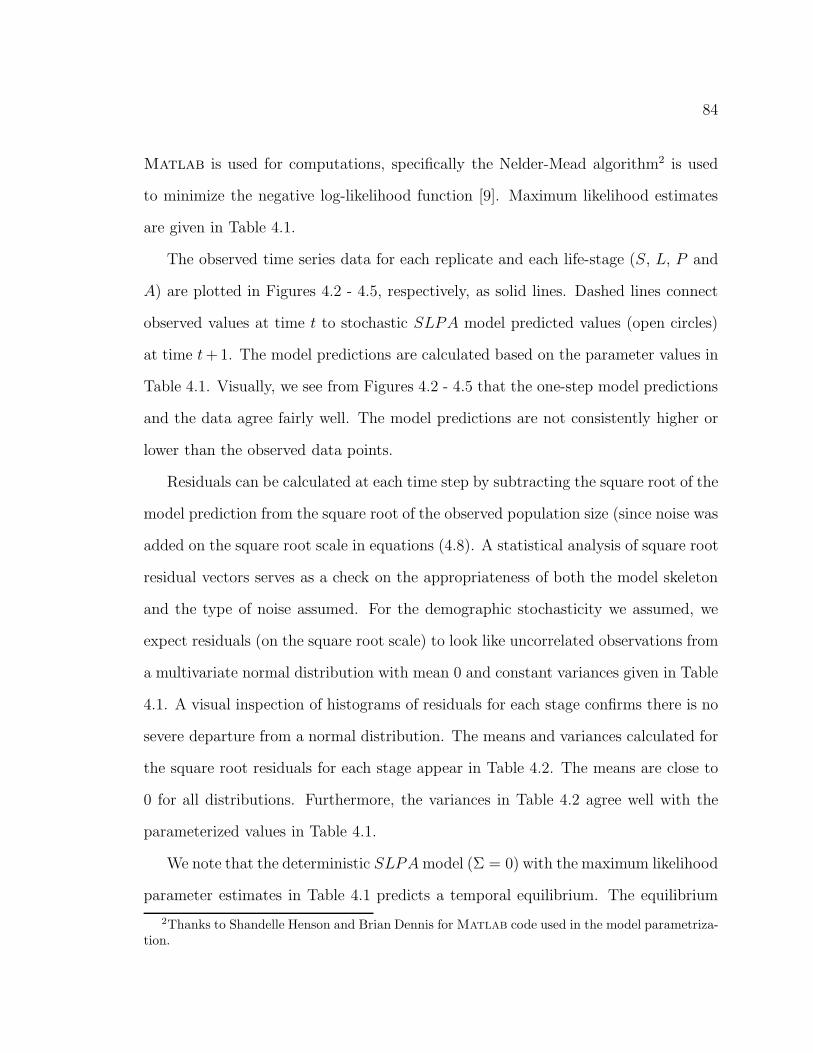
84
Matlab is used for computations, specifically the Nelder-Mead algorithm2 is used
to minimize the negative log-likelihood function [9]. Maximum likelihood estimates
are given in Table 4.1.
The observed time series data for each replicate and each life-stage (S, L, P and
A) are plotted in Figures 4.2 - 4.5, respectively, as solid lines. Dashed lines connect
observed values at time t to stochastic SLPA model predicted values (open circles)
at time t +1. The model predictions are calculated based on the parameter values in
Table 4.1. Visually, we see from Figures 4.2 - 4.5 that the one-step model predictions
and the data agree fairly well. The model predictions are not consistently higher or
lower than the observed data points.
Residuals can be calculated at each time step by subtracting the square root of the
model prediction from the square root of the observed population size (since noise was
added on the square root scale in equations (4.8). A statistical analysis of square root
residual vectors serves as a check on the appropriateness of both the model skeleton
and the type of noise assumed. For the demographic stochasticity we assumed, we
expect residuals (on the square root scale) to look like uncorrelated observations from
a multivariate normal distribution with mean 0 and constant variances given in Table
4.1. A visual inspection of histograms of residuals for each stage confirms there is no
severe departure from a normal distribution. The means and variances calculated for
the square root residuals for each stage appear in Table 4.2. The means are close to
0 for all distributions. Furthermore, the variances in Table 4.2 agree well with the
parameterized values in Table 4.1.
We note that the deterministic SLPA model (Σ = 0) with the maximum likelihood
parameter estimates in Table 4.1 predicts a temporal equilibrium. The equilibrium
2Thanks to Shandelle Henson and Brian Dennis for Matlab code used in the model parametriza-tion.

85
Table 4.1: Maximum likelihood parameter estimates for the stochastic SLPA model(4.8).
Parameter Estimate
b 11.4096ces 0.0135cel 0.0169cea 0.0223µL 0.1339ki 0.0194µ∗
A 0.0158σ2
11 3.553σ2
22 2.8545σ2
33 4.3776σ2
44 0.4865
stage vector is (S∗, L∗, P ∗, A∗) = (12.21, 71.77, 2.59, 163.84).
Calculations show that as the inhibition parameter ki increases, all other param-
eters remaining fixed, the number of large larvae equilibrium stage vector increases
and eventually L is the dominant stage with L∗ > A∗.
4.2.3 The Spatial SLPA Model
To consider a spatial extension of the SLPA model for T. brevicornis, we need to first
define a spatial domain. Although the patterns observed in T. brevicornis (see Figures
1.2, 1.5, 1.4) have all been on a two-dimensional surface, we will take advantage of
an approximate cross-sectional symmetry in some patterns observed in T. brevicornis
and consider one spatial dimension.
We also need to consider what form the dispersal kernel should have. As the
observed patterns are on the surface of the flour container (unlike when we were
considering depth of flour in Ghent’s experiment) there are no inherent heterogeneities
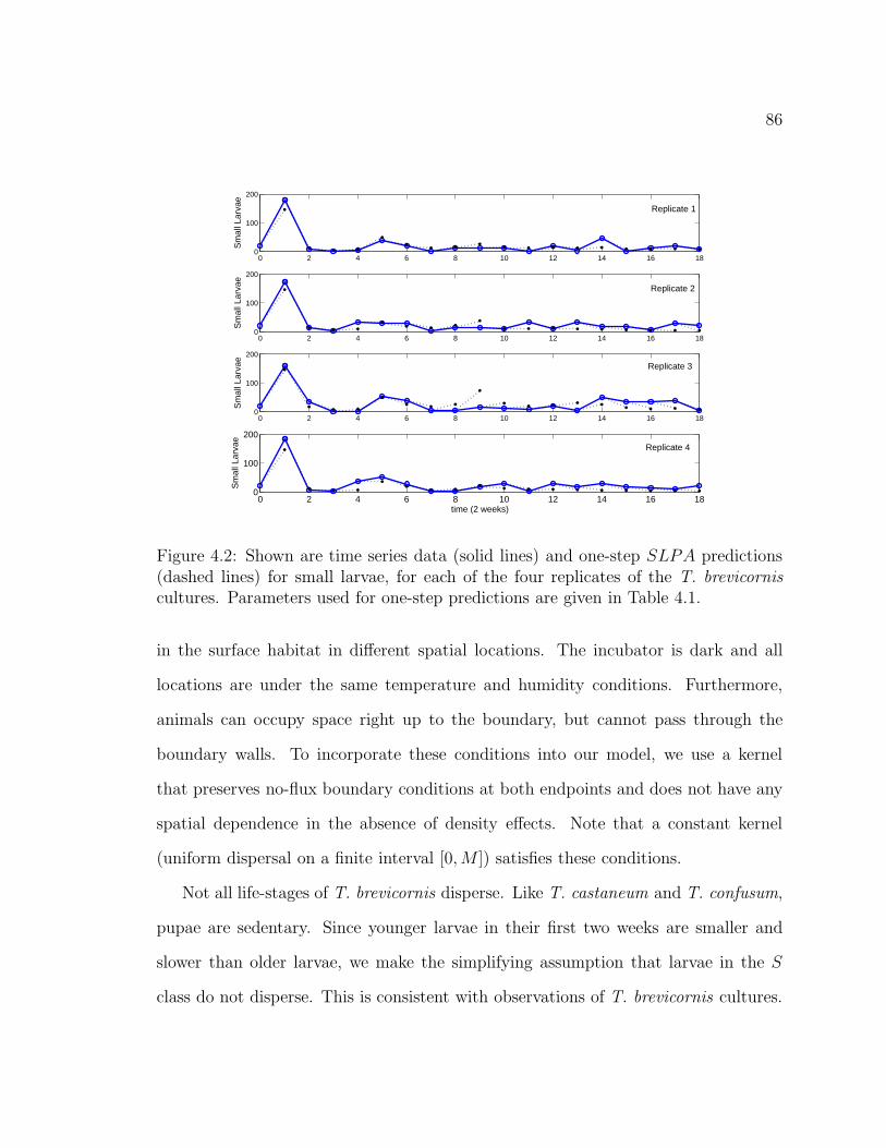
86
0 2 4 6 8 10 12 14 16 180
100
200
Sm
all L
arva
e
0 2 4 6 8 10 12 14 16 180
100
200
Sm
all L
arva
e
0 2 4 6 8 10 12 14 16 180
100
200
Sm
all L
arva
e
0 2 4 6 8 10 12 14 16 180
100
200
Sm
all L
arva
e
time (2 weeks)
Replicate 2
Replicate 1
Replicate 4
Replicate 3
Figure 4.2: Shown are time series data (solid lines) and one-step SLPA predictions(dashed lines) for small larvae, for each of the four replicates of the T. brevicornis
cultures. Parameters used for one-step predictions are given in Table 4.1.
in the surface habitat in different spatial locations. The incubator is dark and all
locations are under the same temperature and humidity conditions. Furthermore,
animals can occupy space right up to the boundary, but cannot pass through the
boundary walls. To incorporate these conditions into our model, we use a kernel
that preserves no-flux boundary conditions at both endpoints and does not have any
spatial dependence in the absence of density effects. Note that a constant kernel
(uniform dispersal on a finite interval [0, M ]) satisfies these conditions.
Not all life-stages of T. brevicornis disperse. Like T. castaneum and T. confusum,
pupae are sedentary. Since younger larvae in their first two weeks are smaller and
slower than older larvae, we make the simplifying assumption that larvae in the S
class do not disperse. This is consistent with observations of T. brevicornis cultures.
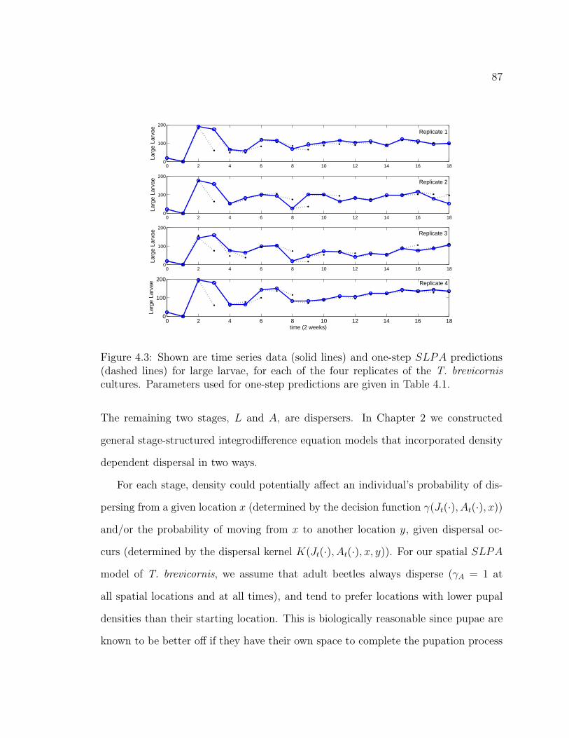
87
0 2 4 6 8 10 12 14 16 180
100
200
Larg
e La
rvae
0 2 4 6 8 10 12 14 16 180
100
200
Larg
e La
rvae
0 2 4 6 8 10 12 14 16 180
100
200
Larg
e La
rvae
0 2 4 6 8 10 12 14 16 180
100
200
time (2 weeks)
Larg
e La
rvae
Replicate 1
Replicate 2
Replicate 3
Replicate 4
Figure 4.3: Shown are time series data (solid lines) and one-step SLPA predictions(dashed lines) for large larvae, for each of the four replicates of the T. brevicornis
cultures. Parameters used for one-step predictions are given in Table 4.1.
The remaining two stages, L and A, are dispersers. In Chapter 2 we constructed
general stage-structured integrodifference equation models that incorporated density
dependent dispersal in two ways.
For each stage, density could potentially affect an individual’s probability of dis-
persing from a given location x (determined by the decision function γ(Jt(·), At(·), x))
and/or the probability of moving from x to another location y, given dispersal oc-
curs (determined by the dispersal kernel K(Jt(·), At(·), x, y)). For our spatial SLPA
model of T. brevicornis, we assume that adult beetles always disperse (γA = 1 at
all spatial locations and at all times), and tend to prefer locations with lower pupal
densities than their starting location. This is biologically reasonable since pupae are
known to be better off if they have their own space to complete the pupation process

88
0 2 4 6 8 10 12 14 16 180
50
100
150
Pup
ae
0 2 4 6 8 10 12 14 16 180
50
100
150
Pup
ae
0 2 4 6 8 10 12 14 16 180
50
100
Pup
ae
0 2 4 6 8 10 12 14 16 180
50
100
150
time (2 weeks)
Pup
ae
Replicate 4
Replicate 3
Replicate 2
Replicate 1
Figure 4.4: Shown are time series data (solid lines) and one-step SLPA predictions(dashed lines) for pupae, for each of the four replicates of the T. brevicornis cultures.Parameters used for one-step predictions are given in Table 4.1.
and do not have other stages crawling over them. Recall T. brevicornis adults do
not cannibalize pupae and have no reason to actively seek them out. We incorporate
density dependent dispersal into the adult kernel by multiplying our constant density
independent kernel by an exponentially decreasing function of pupal density. Thus
we assume adult dispersal is governed by the following kernel, where KA gives the
fraction of adults that move from their starting location to location x:
KA =1
Cexp(−DAP ((1 − µL) exp(−kiAt(x))Lt(x)))
γA = 1
(4.12)
where C is a normalization constant. We also assume that large larvae have no reason
to avoid small larvae or pupae. However, if adult densities are too great, the large
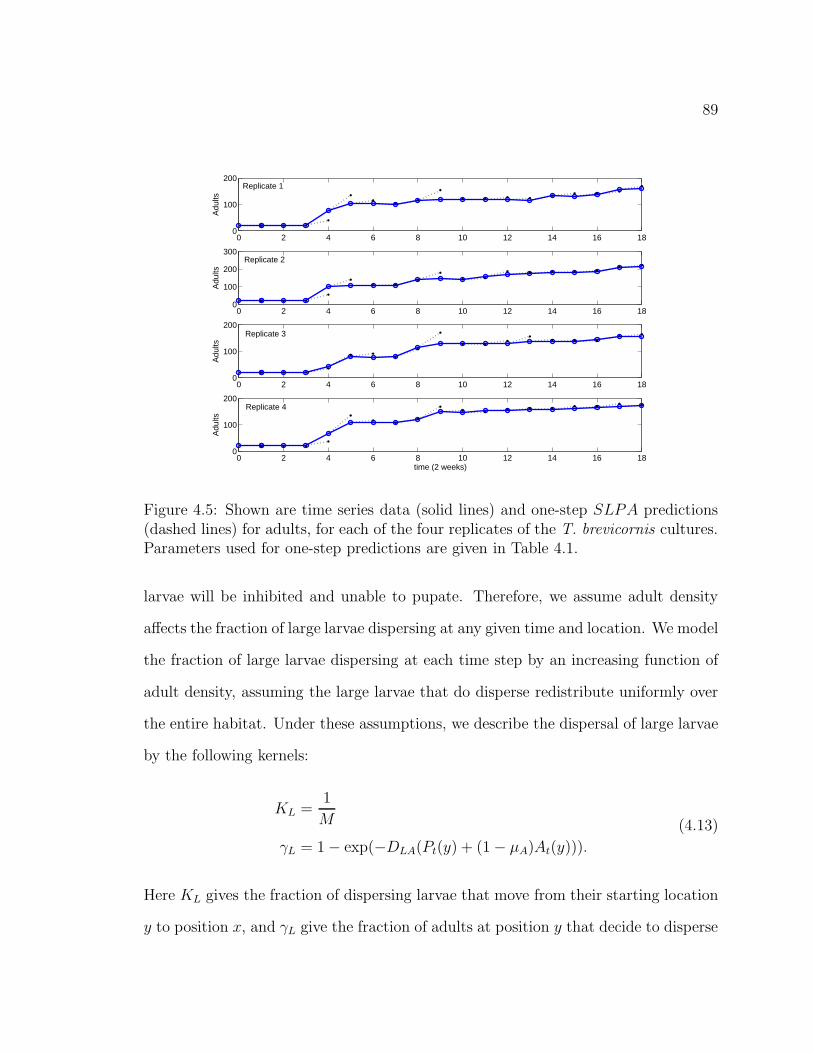
89
0 2 4 6 8 10 12 14 16 180
100
200
Adu
lts
0 2 4 6 8 10 12 14 16 180
100
200
300
Adu
lts
0 2 4 6 8 10 12 14 16 180
100
200
Adu
lts
0 2 4 6 8 10 12 14 16 180
100
200
time (2 weeks)
Adu
lts
Replicate 1
Replicate 2
Replicate 3
Replicate 4
Figure 4.5: Shown are time series data (solid lines) and one-step SLPA predictions(dashed lines) for adults, for each of the four replicates of the T. brevicornis cultures.Parameters used for one-step predictions are given in Table 4.1.
larvae will be inhibited and unable to pupate. Therefore, we assume adult density
affects the fraction of large larvae dispersing at any given time and location. We model
the fraction of large larvae dispersing at each time step by an increasing function of
adult density, assuming the large larvae that do disperse redistribute uniformly over
the entire habitat. Under these assumptions, we describe the dispersal of large larvae
by the following kernels:
KL =1
M
γL = 1 − exp(−DLA(Pt(y) + (1 − µA)At(y))).
(4.13)
Here KL gives the fraction of dispersing larvae that move from their starting location
y to position x, and γL give the fraction of adults at position y that decide to disperse

90
Table 4.2: Residual Analysis. Means and variances for the square root residuals forstages S, L, P and A. Untransformed residuals can be seen in Figures 4.2-4.5, as thedifference between the model prediction and observed stage vector at each time-step.Maximum likelihood estimates for the variances of the transformed residuals are givenin Table 4.1.
Stage Mean Variance
S 0.158 3.576L 0.412 2.723P 0.194 4.402A -0.136 0.4746
at a given time. The decision function γL is plotted in Figure 4.6 for several values
of the parameter DLA. The fraction of larvae leaving a given location and time is a
function of the density of adults present at that location and time.
Combining the dispersal kernel, decision functions, and SLPA population dynam-
ics, we arrive at a spatial SLPA integrodifference equation model on the homogenous
spatial domain Ω = [0, M ]:
St+1(x) = bAt(x)e−cesSt(x)−celLt(x)−ceaAt(x)
Lt+1(x) =
∫ M
0
1
M(1 − e−DLA(Pt(y)+(1−µA)At(y)))×
(St(y) + (1 − µL)(1 − e−kiAt(y))Lt(y))dy
+ e−DLA(Pt(x)+(1−µA)At(x))(St(x) + (1 − µL)(1 − e−kiAt(x))Lt(x))
Pt+1(x) = (1 − µL)e−kiAt(x)Lt(x)
At+1(x) =
∫ M
0
1
Ce−DAP ((1−µL)e−kiAt(x)Lt(x))(Pt(y) + (1 − µA)At(y))dy.
(4.14)
To simulate this model, we must choose initial conditions that satisfy our no-flux
boundary conditions. An initial condition with a uniform spatial distribution will
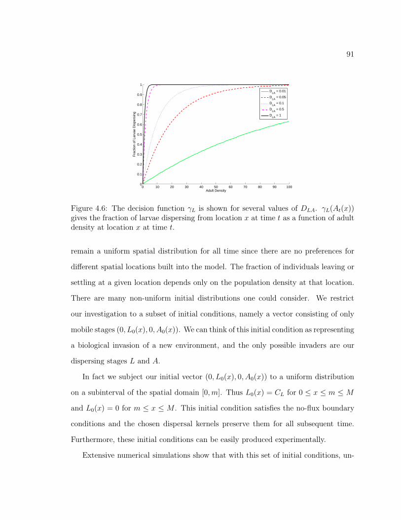
91
0 10 20 30 40 50 60 70 80 90 1000
0.1
0.2
0.3
0.4
0.5
0.6
0.7
0.8
0.9
1
Adult Density
Fra
ctio
n of
Lar
vae
Dis
pers
ing
DLA
= 0.01
DLA
= 0.05
DLA
= 0.1
DLA
= 0.5
DLA
= 1
Figure 4.6: The decision function γL is shown for several values of DLA. γL(At(x))gives the fraction of larvae dispersing from location x at time t as a function of adultdensity at location x at time t.
remain a uniform spatial distribution for all time since there are no preferences for
different spatial locations built into the model. The fraction of individuals leaving or
settling at a given location depends only on the population density at that location.
There are many non-uniform initial distributions one could consider. We restrict
our investigation to a subset of initial conditions, namely a vector consisting of only
mobile stages (0, L0(x), 0, A0(x)). We can think of this initial condition as representing
a biological invasion of a new environment, and the only possible invaders are our
dispersing stages L and A.
In fact we subject our initial vector (0, L0(x), 0, A0(x)) to a uniform distribution
on a subinterval of the spatial domain [0, m]. Thus L0(x) = CL for 0 ≤ x ≤ m ≤ M
and L0(x) = 0 for m ≤ x ≤ M . This initial condition satisfies the no-flux boundary
conditions and the chosen dispersal kernels preserve them for all subsequent time.
Furthermore, these initial conditions can be easily produced experimentally.
Extensive numerical simulations show that with this set of initial conditions, un-
92
der the maximum likelihood SLPA model parameter estimates obtained above, the
spatial SLPA model admits multiple attractors. These attractors include a spatially
uniform distribution and a “patchy” distribution. The patchy attractor consists of a
spatially uniform equilibrium (Se, Le, Pe, Ae) on [0, m] and a spatially uniform equi-
librium (S∗e , L
∗e, P
∗e , A∗
e) on [m, M ]. For DAP large enough, adults are completely
restricted to either [0, m] or [m, M ] and are completely absent in the other patch.
Thus, the model predicts that pupae form a “nest,” i.e. a patch of pupae not occu-
pied by adults. As we will see below, these nests have been observed in experimental
cultures of T. brevicornis.
Initial conditions leading to each attractor vary with parameter values. For exam-
ple, the initial condition of L0(x) = 0, A0(x) = 100 on the left quarter of the domain2
[0, 14] leads to a patchy attractor for many values of ki, including ki = 0.01, 0.0194,
0.05, and 0.07. For these same values of ki, an initial condition of L0(x) = 100,
A0(x) = 0 for x ∈ [0, 14] leads to a spatially uniform attractor.
When inhibition is absent (ki = 0) the patchy distribution is either extremely
rare or never present. Most initial conditions lead to a spatially uniform distribution.
This suggests that inhibition is necessary for the segregation of life cycle stages in a
homogenous habitat.
These findings are illustrated in Figure 4.7 and Figure 4.8, which show the uniform
and patch attractors resulting from the same set of parameter values (given in figure
captions), but different initial conditions. In Figure 4.7 the initial conditions are
L0(x) = 100, A0(x) = 0 for x ∈ [0, 14] and the attractor is a spatially uniform
equilibrium with (Se, Le, Pe, Ae) = (12.21, 71.77, 2.59, 163.8). In Figure 4.8, the initial
conditions are L0(x) = 0, A0(x) = 100 for x ∈ [0, 14], and the result is a two patch
2Domain size M does not affect model attractors, only total population size. M = 1 and m = 1
4
were used for simulations in this chapter.
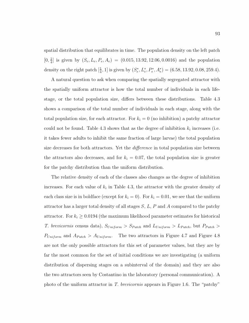
93
spatial distribution that equilibrates in time. The population density on the left patch
[0, 14] is given by (Se, Le, Pe, Ae) = (0.015, 13.92, 12.06, 0.0016) and the population
density on the right patch [14, 1] is given by (S∗
e , L∗e, P
∗e , A∗
e) = (6.58, 13.92, 0.08, 259.4).
A natural question to ask when comparing the spatially segregated attractor with
the spatially uniform attractor is how the total number of individuals in each life-
stage, or the total population size, differs between these distributions. Table 4.3
shows a comparison of the total number of individuals in each stage, along with the
total population size, for each attractor. For ki = 0 (no inhibition) a patchy attractor
could not be found. Table 4.3 shows that as the degree of inhibition ki increases (i.e.
it takes fewer adults to inhibit the same fraction of large larvae) the total population
size decreases for both attractors. Yet the difference in total population size between
the attractors also decreases, and for ki = 0.07, the total population size is greater
for the patchy distribution than the uniform distribution.
The relative density of each of the classes also changes as the degree of inhibition
increases. For each value of ki in Table 4.3, the attractor with the greater density of
each class size is in boldface (except for ki = 0). For ki = 0.01, we see that the uniform
attractor has a larger total density of all stages S, L, P and A compared to the patchy
attractor. For ki ≥ 0.0194 (the maximum likelihood parameter estimates for historical
T. brevicornis census data), SUniform > SPatch and LUniform > LPatch, but PPatch >
PUniform and APatch > AUniform. The two attractors in Figure 4.7 and Figure 4.8
are not the only possible attractors for this set of parameter values, but they are by
far the most common for the set of initial conditions we are investigating (a uniform
distribution of dispersing stages on a subinterval of the domain) and they are also
the two attractors seen by Costantino in the laboratory (personal communication). A
photo of the uniform attractor in T. brevicornis appears in Figure 1.6. The “patchy”
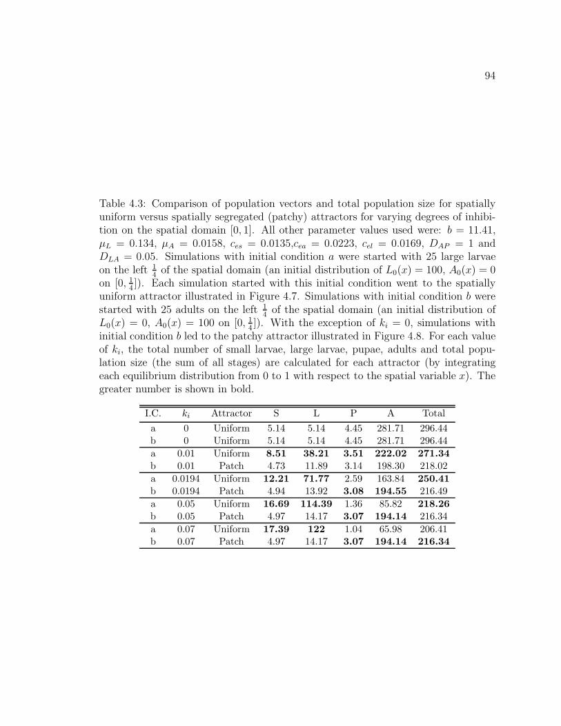
94
Table 4.3: Comparison of population vectors and total population size for spatiallyuniform versus spatially segregated (patchy) attractors for varying degrees of inhibi-tion on the spatial domain [0, 1]. All other parameter values used were: b = 11.41,µL = 0.134, µA = 0.0158, ces = 0.0135,cea = 0.0223, cel = 0.0169, DAP = 1 andDLA = 0.05. Simulations with initial condition a were started with 25 large larvaeon the left 1
4of the spatial domain (an initial distribution of L0(x) = 100, A0(x) = 0
on [0, 14]). Each simulation started with this initial condition went to the spatially
uniform attractor illustrated in Figure 4.7. Simulations with initial condition b werestarted with 25 adults on the left 1
4of the spatial domain (an initial distribution of
L0(x) = 0, A0(x) = 100 on [0, 14]). With the exception of ki = 0, simulations with
initial condition b led to the patchy attractor illustrated in Figure 4.8. For each valueof ki, the total number of small larvae, large larvae, pupae, adults and total popu-lation size (the sum of all stages) are calculated for each attractor (by integratingeach equilibrium distribution from 0 to 1 with respect to the spatial variable x). Thegreater number is shown in bold.
I.C. ki Attractor S L P A Total
a 0 Uniform 5.14 5.14 4.45 281.71 296.44b 0 Uniform 5.14 5.14 4.45 281.71 296.44
a 0.01 Uniform 8.51 38.21 3.51 222.02 271.34
b 0.01 Patch 4.73 11.89 3.14 198.30 218.02
a 0.0194 Uniform 12.21 71.77 2.59 163.84 250.41
b 0.0194 Patch 4.94 13.92 3.08 194.55 216.49
a 0.05 Uniform 16.69 114.39 1.36 85.82 218.26
b 0.05 Patch 4.97 14.17 3.07 194.14 216.34
a 0.07 Uniform 17.39 122 1.04 65.98 206.41b 0.07 Patch 4.97 14.17 3.07 194.14 216.34
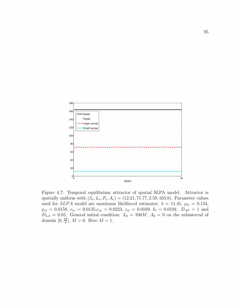
95
0 M0
20
40
60
80
100
120
140
160
180
Space
Adults
Pupae
Large Larvae
Small Larvae
Figure 4.7: Temporal equilibrium attractor of spatial SLPA model. Attractor isspatially uniform with (Se, Le, Pe, Ae) = (12.21, 71.77, 2.59, 163.8). Parameter valuesused for SLPA model are maximum likelihood estimates: b = 11.41, µL = 0.134,µA = 0.0158, ces = 0.0135,cea = 0.0223, cel = 0.0169, ki = 0.0194. DAP = 1 andDLA = 0.05. General initial condition: L0 = 100M , A0 = 0 on the subinterval ofdomain [0, M
4], M > 0. Here M = 1.
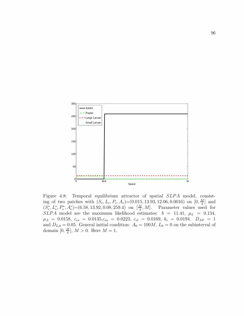
96
0 M/4 M0
50
100
150
200
250
300
Space
Adults
Pupae
Large Larvae
Small Larvae
Figure 4.8: Temporal equilibrium attractor of spatial SLPA model, consist-ing of two patches with (Se, Le, Pe, Ae)=(0.015, 13.93, 12.06, 0.0016) on [0, M
4] and
(S∗e , L
∗e, P
∗e , A∗
e)=(6.58, 13.92, 0.08, 259.4) on [M4, M ]. Parameter values used for
SLPA model are the maximum likelihood estimates: b = 11.41, µL = 0.134,µA = 0.0158, ces = 0.0135,cea = 0.0223, cel = 0.0169, ki = 0.0194. DAP = 1and DLA = 0.05. General initial condition: A0 = 100M , L0 = 0 on the subinterval ofdomain [0, M
4], M > 0. Here M = 1.

97
attractor, and the establishment of a pupal nest by T. brevicornis, can be seen in
Figures 1.5 and 1.4.
The culture in Figure 1.6 was started with T. brevicornis adults in the upper
right corner of the box. The adults immediately spread out and no pupal nest was
ever established. To simulate this situation where adults are immediately allowed to
disperse, the spatial SLPA model needs to be started with an initial condition of
only L stage individuals. Since reproduction occurs before dispersal in the model,
L stage individuals will all pupate immediately (since no A stage individuals are
present to delay pupation) and emerge as adults. These adults will then disperse
according to equation (4.12), the adult dispersal kernel. The absence of pupae results
in the adults dispersing uniformly throughout the entire domain, matching what is
seen experimentally. Therefore, a laboratory initial condition of only adults who are
immediately permitted to disperse corresponds to a model simulation initial condition
of only large larvae. In two time steps this initial condition will result in a cohort of
dispersing adults, with no other stages present.
The three cultures in Figure 1.4 were started with L and A stage animals mixed
together on the left half of the domain. The movement of these animals was restricted
by a panel inserted to divide each row of flour in half. After 6 weeks the panel was
removed and animals were able to migrate into the right half of each row. This
resulted in the formation of a pupal nest. Such a patchy attractor can be predicted
by the model for initial conditions of adults only, or of both adults and large larvae.
Since reproduction occurs before dispersal in the model, the initial condition of A
only results in A and S stage individuals present at the time of dispersal. The small
larvae do not disperse, but the A spread out across the entire domain. The next
time step, small larvae become large larvae. These large larvae will not disperse

98
provided the adult density is low enough (this depends on the decision parameter
DLA) from the adults spreading out over the entire habitat. At the next time step,
these same large larvae will pupate in their original location if adult density is low
enough (this depends on the inhibition parameter ki). Once they do, a pupal nest
has been established and it will be avoided by the adults in subsequent time steps.
If the model is instead started with both L and A stage individuals present, a
situation similar to the one just described (for an initial condition of A only) occurs.
The initial density of A may be great enough to inhibit large larvae. If so, a fraction
of them, determined by γL, will disperse uniformly over the whole domain along with
the adults. The next time step, adults should be spread out enough to allow all large
larvae to pupate. Unless all L dispersed, the density of L should be greater in their
starting interval than the rest of the domain and this will result in a greater density
of pupae and mark the location of the pupal nest. The moment the door is opened
in the laboratory culture corresponds to halfway through a model time step - after
reproduction but right before dispersal.
Over time, the nest persists both in model simulations (since the patchy attractor
is a temporal equilibrium attractor) and laboratory cultures, in the location it was
originally established. This location does not have to be at the edge of the domain; it
can be an interval in the center of the domain as well. Adults can become very dense
outside of the nest, and this may provide a barrier to any invading species, including
those where adults cannibalize pupae. Costantino has hypothesized that the pupal
nest together with the adult barrier surrounding it may serve to protect the pupae
this species has invested so much time into developing (personal communication).
In summary, the spatial SLPA model (4.8) has been able to predict observed
spatial segregation in T. brevicornis. We were able to further connect model (4.8)
99
with experimental observations for select cases, providing experimental support for
the multiple spatial attractors predicted by the spatial SLPA model. The fact that
we were unable to find initial conditions leading to the patchy attractor when the
inhibition parameter ki = 0 suggests that the inhibition of large larvae is a necessary
condition for spatial segregation of life cycle stages. This is consistent with the absence
of surface patterns in non-inhibiting species such as T. castaneum and T. confusum.
Furthermore, the model predicts that for a species with the parameterized inhibition
level of T. brevicornis (ki = 0.0194), the spatial separation of life cycle stages can
affect the relative total population sizes of the stages. Specifically, the total number of
pupae and adults are higher for the patchy attractor relative to the uniform attractor.
Sexually mature adults become the dominant stage in the patchy attractor, whereas
the immature large larvae dominate for the spatially uniform attractor.
100
Chapter 5
Concluding Remarks
We have shown that density dependent dispersal can lead to the segregation of life
cycle stages in stage-structured populations (such as flour beetles), and furthermore
that these patterns can occur in both homogenous and heterogeneous spatial envi-
ronments. These results are not intuitively obvious. In the case of a juvenile-adult
species, even if juvenile avoid adults and adults avoid juveniles, juveniles will even-
tually become adults and adults will give rise to new juveniles, seemingly leading to
spatial mixing between stages.
In chapter 1 we reference spatial habitat segregation as a potential adaptation to
avoid cannibalism or predation. In Tribolium, larvae are not being directly cannibal-
ized by the adults but density dependent dispersal, and the avoidance of adults, may
still be a beneficial adaptation. T. castaneum and T. confusum pupae are cannibal-
ized by adults, so if larvae pupate in a location inhabited by a large number of adults,
they may not survive the pupal stage. T. brevicornis pupae, on the other hand, are
not eaten by adults. These larvae have a different reason to escape adults - inhibited
pupation caused by the presence of adults. Large larvae cannot complete their life
cycle if too many adults are nearby.
Based on our studies we also hypothesize about mechanisms that promote adult
dispersal. Eggs of both species are cannibalized by larvae, and the adults may want
to lay their eggs in flour where they have the greatest chance of hatching, and where
there is the greatest food supply once their young become larvae. This is our rationale
101
for adults avoiding larvae in the dispersal kernels in our model for T. confusum and T.
castaneum. For T. brevicornis, the adult avoidance of larvae does not lead to spatial
segregation of adults and other life stages. In this species, segregation is obtained
when the adults avoid the P stage, which includes pre-pupae. This species devotes
more time to the larval stage than T. confusum and T. castaneum, spending at least
four weeks as a larvae rather than only two. If larvae are inhibited, they may spend
months in the larval stage. After investing so much time in the larval stage, the
species takes great care of their pupae. Adults leave them alone, since crawling over
them can decrease the chances they will emerge as a healthy adult.
The toy models in Chapter 3 show that density dependent dispersal can result
in both spatial segregation of life cycle stages as well as temporal segregation (if
mortality is associated with dispersal). We stress that complex population dynamics
are not necessary for the formation of these spatial patterns and that our models do
not result in spatial segregation in the absence of density dependent dispersal (as long
as all mobile stages “view” the environment the same way).
In Chapter 4 we considered two biological applications of the spatial models devel-
oped in Chapters 2 and 3. First, we aimed to explain the uneven depth distribution of
larval and adult flour beetles of the species T. castaneum and T. confusum observed
by Ghent [14]. Due to gravity, flour is more dense at the bottom of a vial of flour
than at the top, and most likely less desirable an environment to beetles than the
less dense flour near the surface. We modeled this biological system assuming no-flux
boundary conditions at the surface and hostile boundary conditions at the bottom of
the bottle, as well as the density dependent dispersal of adults and larva (assuming
adults avoid larvae and visa versa). Even though larvae and adults have the same
spatial preferences, the adults end up with higher densities in the preferred flour.
102
Larvae and pupae appear to be “pushed” towards the bottom of the bottle. These
model predicted results agree qualitatively with what Ghent observed (Figure 1.1).
It is also of note that the lower dimensional juvenile-adult spatial model with mixed
boundary conditions considered in Chapter 3 also results in adults dominating near
the surface and juveniles reaching their maximum density at lower depths.
We do not expect quantitative agreements between our results and those of Ghent
for multiple reasons. First, parameter values for flour beetle populations can vary from
strain to strain, and we do not have parameter values for the strain used by Ghent.
Second, the vials used by Ghent held 8 grams of flour, while the typical bottles used
in experiments and parametrization of the LPA model held 20 grams of flour [7, 9].
Also, Ghent’s data was collected after 26 days in the vial, not long enough for new
adults to emerge. Our results are asymptotic model attractors.
As discussed in Chapter 1, there is literature to support the density dependent
dispersal of flour beetles, but the exact mechanisms and rates of dispersal are un-
known. Our results do show that our hypothesized density dependent interactions
and the resulting dispersal kernels are possible explanations for the observed spatial
distributions. The main message of this case study is that density dependent disper-
sal can produce a spatial pattern very similar to that observed by Ghent and may
have been a factor in its development.
The patterns observed in our second case study species, T. brevicornis, are more
striking than the subtle depth differences observed by Ghent. Adults clearly clump
together, a behavior not seen by Costantino or noted in the literature for any other
Tribolium species, even other inhibiting species such as T. freemani. However, T.
freemani larvae are inhibited by both larvae and adults, so escaping high densities of
adults alone would not help them pupate. In fact, laboratory cultures of this species

103
almost always result in a strong larval bottleneck with very few adults present. In
T. brevicornis, on the other hand, when larvae escape to areas of low adult density
they immediately pupate (provided they are old enough). Mathematically, inhibition
plays an important role in the formation of spatial segregation. The number of initial
conditions giving rise to the patchy attractor of the spatial SLPA model decreases as
the severity of inhibition decreases. In fact, the patchy attractor could not be found
when the inhibition parameter ki was set to zero.
A potential benefit of density dependent dispersal for inhibiting species lies in
population size and structure of the stage-class vector. All other parameters equal,
the model always predicts a non-inhibitor will have greater total population sizes
than an inhibiting species. This makes sense intuitively, since 100% of larva surviving
mortality go on to pupate in the absence of inhibition. Inhibition only decreases this
number and can only decrease total population size. Using this criteria, inhibition
appears to put a species at a disadvantage.
We also compared population numbers for an inhibiting species in two differ-
ent spatial structures. We found that if inhibition is strong enough, the spatially
segregated model attractor has a greater population size than the spatially uniform
attractor. This also makes biological sense. If a species is a strong inhibitor, very
few larvae will be able to pupate once an adult cohort has been established. Eggs
will still be laid but few new sexually mature adults will be established. The model
shows that separating the stages spatially and giving the larvae a refuge to pupate
results in higher population numbers, which is typically considered to be biologically
beneficial for the population.
For the parameterized inhibition level of T. brevicornis, spatial segregation does
not quite result in greater total population numbers, but it does shift the composition

104
of the equilibrium stage vector (S∗, L∗, P ∗, A∗) in favor of higher numbers of P ∗ and
A∗. Increasing the number of sexually mature adults in a population is also often
seen as biologically beneficial. If dispersal is really important in this species’ natural
habitat, adults may be the primary invaders of new colonies. Increasing the number
of adults could mean larger founding populations at their next location.
As noted above, the spatial SLPA model exhibits multiple attractors, including a
spatially uniform attractor and a “patchy” attractor with pupae and adults spatially
separated. These two attractors have been seen in experimental cultures of T. brevi-
cornis. The spatial segregation of adults and other life cycle stages has been observed
in many different sizes and shapes of T. brevicornis cultures, as seen in Figures 1.2,
1.5 and 1.4. However, the shape of the surface of the container used in Figures 1.5 and
1.4 is the closest to being one-dimensional and also produces the most reproducible
patterns. Vertical cross sections through each row yield an approximately uniform
distribution of beetles and so the pattern can be collapsed to one dimension more
easily than those in Figure 1.2.
Figures 1.5 and 1.4 clearly show the formation of the pupal nest that is predicted by
the patchy attractor of the spatial SLPA model, while Figure 1.6 shows the uniform
attractor of the spatial SLPA model. As discussed in Chapter 4.2, initial conditions
for the laboratory cultures are consistent with those used in model simulations. A
patchy attractor is reached if a pupal nest has a chance to be established. If a culture
is started with adults who immediately have the opportunity to disperse, they spread
out, taking advantage of the entire habitat. If a culture is started with large larvae
and adults who are contained in a subsection of the habitat, the adults inhibit the
large larvae and prevent them from pupating. Once the “door” is opened, allowing
them to access to the entire habitat, the adults disperse quickly. The large larvae
105
don’t get very far before sensing conditions are right to pupate, and a pupal nest is
established. Once the nest is established, it persists over time. New adults emerge and
leave the nest, while large larvae from outside the nest have been observed returning
to the nest.
5.1 Future Investigations
The integrodifference equation models we investigated thus far have been one di-
mensional in space. The observed patterns used to motivate our studies are higher
dimensional. While the patterns in Ghent’s experiments and in each of the rows in
Figure 1.4 can reasonably be collapsed to an approximately one dimensional distribu-
tion, the surface patterns shown in Figure 1.2 are definitely two dimensional surface
patterns. A two dimensional spatial model may be able to explain patterns such as
the “beetle butterfly” seen in Figure 1.2b. Mathematically, the models can easily be
extended to two dimensional spatial domains, and the bifurcation theory developed
in Chapter 2 applied in any spatial dimension. However, model simulations become
much more computationally intensive.
All our spatial LPA and SLPA model simulations were done on a one dimensional
domain consisting of a closed finite interval. An assumption in the formation of the
kernels for the spatial LPA and SLPA models was that all dispersing animals could
cover the entire habitat in one time step. We have not considered the role of domain
size in the formation of spatial patterns for these models. (We did, however, consider
domain size in the “toy” juvenile-adult models in Chapter 3, observed that spatial
segregation does not occur if the domain is too small.) Domain size and/or dispersal
speed may play an important role in the formation of spatial patterns of species
106
exhibiting density dependent dispersal on a larger domain. It would be interesting to
study larger domains which dispersers cannot cover in one time period.
Our results may have important implications for future multi-species competition
studies. Many experiments have been done on the subject of competition between
closely related species [29]. In cultures of T. confusum and T. castaneum, almost
all cultures saw one species exclude the other according to the principle of competi-
tive exclusion. The winning species depended on initial conditions. The LPA model
has had previous success modeling competition; an extension of the LPA model to a
competition model has led to potential counterexamples to the principle of competi-
tive exclusion, explaining prolonged coexistence between two species of closely related
flour beetles observed by Park [13].
Jillson and Costantino experimented with competition between T. brevicornis and
T. castaneum. Every culture resulted in competitive exclusion, with T. brevicornis
always being eliminated regardless of initial conditions [4, 21]. Inhibition of T. bre-
vicornis larvae is not species specific, so contact with T. castaneum adults will also
delay pupal metamorphosis [21]. Furthermore, T. castaneum adults will cannibalize
T. brevicornis pupae in addition to their own. Thus, T. brevicornis has a two-fold
disadvantage. Their larvae are inhibited by both species’ adults and their larvae that
do manage to pupate are now subject to cannibalism.
The nest of pupae established by T. brevicornis seen in Figure 1.5 does not contain
any nutritious flour. Instead the flour is so highly conditioned it is toxic. This makes
it a perfect place for pupae, as they do not need to eat, and it would provide safety
for T. brevicornis pupae in the presence of cannibalistic T. castaneum adults. As
discussed in Chapter 4.2, the high densities of T. brevicornis adults surrounding the
nest form a barrier for potentially cannibalistic invaders.

107
These factors suggest spatial structure may play an important role when con-
sidering competition between T. brevicornis and a non-inhibiting species such as T.
castaneum or T. confusum. If T. brevicornis has a chance to establish a pupal nest,
the species may be better able to resist an invasion by another flour beetle species.
108
References
[1] Alzoubi, M. Y. A Dispersal Model for Structured Populations. PhD thesis,
University of Arizona, 1999.
[2] Comins, H. N., and Hassell, M. P. Persistence of multispecies host-
parasitoid interactions in spatially distributed models with local dispersal. Jour-
nal of Theoretical Biology 183 (1996), 19–28.
[3] Costantino, R. F., Cushing, J. M., Dennis, B., Desharnais, R. A., and
Henson, S. M. Resonant population cycles in temporally fluctuating habitats.
Bulletin of Mathematical Biology 60, 2 (1998), 247–275.
[4] Costantino, R. F., and Desharnais, R. A. Population Dynamics and the
Tribolium Model: Genetics and Demography. Springer–Verlag, New York, 1991.
[5] Cushing, J. The LPA model. Fields Institute Communications 42 (2004),
29–55.
[6] Cushing, J. M. An Introduction to Structured Population Dynamics,
vol. 71. CBMS-NSF Regional Conference Series in Applied Mathematics, SIAM,
Philadelphia, 1998.
[7] Cushing, J. M., Costantino, R. F., Dennis, B., Desharnais, R. A.,
and Henson, S. M. Chaos in Ecology: Experimental Nonlinear Dynamics,
vol. 1 of Theoretical Ecology Series. Academic Press (Elsevier Science), New
York, 2003.
109
[8] Cushing, J. M., and Yicang, Z. The net reproductive value and stability in
matrix population models. Natural Resource Modeling 8 (1994), 297–333.
[9] Dennis, B., Desharnais, R. A., Cushing, J. M., and Costantino, R. F.
Nonlinear demographic dynamics: Mathematical models, statistical methods,
and biological experiments. Ecological Monographs 65 (1997), 261–281.
[10] Dennis, B., Desharnais, R. A., Cushing, J. M., and Costantino, R. F.
Transitions in population dynamics: equilibria to periodic cycles to aperiodic
cycles. Journal of Animal Ecology 66 (1997), 704–729.
[11] Dennis, B., Desharnais, R. A., Cushing, J. M., Henson, S. M., and
Costantino, R. F. Estimating chaos and complex dynamics in an insect
population. Ecological Monographs 71 (2001), 277–303.
[12] Dwyer, G., and Morris, W. F. Resource-dependent dispersal and the speed
of biological invasions. American Naturalist 167 (2006), 165–176.
[13] Edmunds, J., Cushing, J. M., Costantino, R. F., Henson, S. M., Den-
nis, B., and Desharnais, R. A. Park’s Tribolium competition experiments:
a non-equilibrium species coexistence hypothesis. Journal of Animal Ecology 72
(2003), 703–712.
[14] Ghent, A. W. Studies of behavior of the Tribolium flour beetles. II. Distri-
butions in depth of T. castaneum and T. confusum in fractionable shell vials.
Ecology 47 (1966), 355–367.
[15] Gil’, M. I. Difference Equations in Normed Spaces: Stability and Oscillations.
Elsevier, Amsterdam, 2007.
110
[16] Hardin, D. P., Takac, P., and Webb, G. Asymptotic properties of a
continuous-space discrete-time population model in a random environment. Jour-
nal of Mathematical Biology 26 (1988), 361–374.
[17] Harrison, R. G. Dispersal polymorphisms in insects. Annual Review of Ecology
and Systematics 11 (1980), 95–118.
[18] Hassell, M. P., Comins, H. N., and May, R. M. Spatial structure and
chaos in insect population dynamics. Letters to Nature 353 (1991), 255–258.
[19] Hassell, M. P., Comins, H. N., and May, R. M. Species coexistence and
self-organizing spatial dynamics. Letters to Nature 370 (1994), 290–292.
[20] Hunte, W., and Myers, R. A. Phototaxis and cannibalism in gammaridean
amphipods. Marine Biology 81 (1984), 75–79.
[21] Jillson, D. A., and Costantino, R. F. Growth, distribution, and competi-
tion of Tribolium castaneum and Tribolium brevicornis in fine-grained habitats.
The American Naturalist 116 (1980), 206–219.
[22] Jormalainen, V., and Shuster, S. M. Microhabitat segregation and can-
nibalism in an endangered freshwater isopod, Thermosphaeroma thermophilum.
Oecologia 111 (1997), 271–279.
[23] Kielhofer, H. Bifurcation Theory: An Introduction with Applications to
PDEs. Springer, New York, 2004.
[24] Kisimoto, R. Effect of crowding during the larval period on the determination
of the wing form of an adult plant-hopper. Nature 178 (1956), 641–642.
111
[25] Kot, M., Lewis, M. A., and van den Driessche, P. Dispersal data and
the spread of invading organisms. Ecology 77 (1996), 2027—2042.
[26] Kot, M., and Schaffer, W. Discrete-time growth-dispersal model. Mathe-
matical Biosciences 80 (1986), 109–136.
[27] Krasnosel’skii, M. A. Topological Methods in the Theory of Nonlinear Integral
Equations. Springer, Berlin, 1964.
[28] Leonardsson, K. Effects of cannibalism and alternative prey on population
dynamics of Saduria entomon (Isopoda). Ecology 72 (1991), 1273–1285.
[29] Leslie, P. H., Park, T., and Mertz, D. B. The effect of varying the initial
numbers on the outcome of competition between two Tribolium species. Journal
of Animal Ecology 37 (1968), 9–23.
[30] Levin, S. A. Dispersion and population interactions. American Naturalist 108
(1974), 207–228.
[31] Li, C. K., and Schneider, H. Applications of Perron-Frobenius theory to
population dynamics. Journal of Mathematical Biology 44 (2002), 450–462.
[32] Naylor, A. F. An experimental analysis of dispersal in the flour beetle, Tri-
bolium confusum. Ecology 40 (1959), 453–465.
[33] Naylor, A. F. Dispersal in the red flour beetle Tribolium castaneum (tenebri-
onidae). Ecology 42 (1961), 231–237.
[34] Naylor, A. F. Dispersal responses of female flour beetles, Tribolium confusum,
to presence of larvae. Ecology 46 (1965), 341–343.
112
[35] Neubert, M., Kot, M., and Lewis, M. Dispersal and pattern formation in
a discrete time predator-prey model. Theoretical Population Biology 48 (1994),
7–43.
[36] Neubert, M. G., and Caswell, H. Demography and dispersal: Calculation
and sensitivity analysis of invasion speed for structured populations. Ecology 81
(2000), 1613–1628.
[37] Neyman, J., Park, T., and Scott, E. Struggle for existence. The Tribolium
model: biological and statistical aspects. Proc. 3rd Berkeley Symp. Math. Statist.
Prob. 4 (1956), 41–79.
[38] Prus, T. Emigrational ability and surface numbers of adult beetles in 12 strains
of Tribolium confusum duval and T. castaneum herbst. Ekologia Polska Seria A
14 (1966), 548–588.
[39] Rabinowitz, P. H. Some global results for nonlinear eigenvalue problems.
Journal of Functional Analysis 7 (1971), 1291–1313.
[40] Ribes, M., Coma, R., Zabala, M., and Gili, J. Small scale spatial hetero-
geneity and seasonal variation in a population of a cave-dwelling Mediterannean
mysid. Journal of Plankton Research 18 (1996), 659–671.
[41] Shigesada, N., Kawasaki, K., and Teramoto, E. Spatial segregation of
interacting species. Journal of Theoretical Biology 1979 (1978), 83–99.
[42] Sokoloff, A., Albers, J., Cavataio, P., Mankau, S., McKibben, S.,
Mills, S., Perkins, R., Roberts, L., and Sandri, J. Observations on pop-
ulations of Tribolium brevicornis (Le conte)(Coleoptera, Tenebrionidae). I. Lab-
113
oratory observations of domesticated strains. Researches on Population Ecology
(1980).
[43] Sparrevik, E., and Leonardsson, K. Effects of large Saduria entomon
(isopoda) on spatial distribution of their small S. entomon and Monoporeia affinis
(amphipoda) prey. Oecologia 101 (1995), 177–184.
[44] Van Kirk, R. W., and Lewis, M. A. Integrodifference models for persistence
in fragmented habitats. Bulletin of Mathematical Biology 59 (1997), 107–137.
[45] Veit, R. R., and Lewis, M. A. Dispersal, population growth and the Allee
effect: Dynamics of the house finch invasion of eastern North America. American
Naturalist 148 (1996), 255 – 274.
[46] Wang, M.-H., Kot, M., and Neubert, M. G. Integrodifference equations,
Allee effects, and invasions. Journal of Mathematical Biology 44 (2002), 150–168.
[47] Zeidler, E. Nonlinear Functional Analysis and its Applications I. Springer,
Berlin, 1992.
[48] Ziegler, J. R. Evolution of the migration response: Emigration by Tribolium
and the influence of age. Evolution 30 (1976), 579–592.
[49] Zyromska-Rudzka, H. Abundance and emigrations of Tribolium in a labora-
tory model. Ekologia Polska Seria A 14 (1966), 491–518.