Spatial Pyramid Pooling in Deep Convolutional Networks for Visual RecognitionTechnical report

Kaiming He1 Xiangyu Zhang2∗ Shaoqing Ren3∗ Jian Sun1

1Microsoft Research 2Xi’an Jiaotong University 3University of Science and Technology of China{kahe,jiansun}@microsoft.com xyz.clx@stu.xjtu.edu.cn sqren@mail.ustc.edu.cn

Abstract

Existing deep convolutional neural networks (CNNs) re-quire a fixed-size (e.g. 224×224) input image. This require-ment is “artificial” and may hurt the recognition accuracyfor the images or sub-images of an arbitrary size/scale. Inthis work, we equip the networks with a more principledpooling strategy, “spatial pyramid pooling”, to eliminatethe above requirement. The new network structure, calledSPP-net, can generate a fixed-length representation regard-less of image size/scale. By removing the fixed-size limi-tation, we can improve all CNN-based image classificationmethods in general. Our SPP-net achieves state-of-the-artaccuracy on the datasets of ImageNet 2012, Pascal VOC2007, and Caltech101.

The power of SPP-net is more significant in object detec-tion. Using SPP-net, we compute the feature maps from theentire image only once, and then pool features in arbitraryregions (sub-images) to generate fixed-length representa-tions for training the detectors. This method avoids repeat-edly computing the convolutional features. In processingtest images, our method computes convolutional features30-170× faster than the recent leading method R-CNN (and24-64× faster overall), while achieving better or compara-ble accuracy on Pascal VOC 2007.

1. IntroductionWe are witnessing a rapid, revolutionary change in our

vision community, mainly caused by deep convolutionalneural networks (CNNs) [18] and the availability of largescale training data [6]. Deep-networks-based approacheshave recently been substantially improving upon the stateof the art in image classification [16, 33, 24], object detec-tion [12, 35, 24], many other recognition tasks [23, 27, 34,13], and even non-recognition tasks.

However, there is a technical issue in the training and

∗This work was done when Xiangyu Zhang and Shaoqing Ren wereinterns at Microsoft Research.

crop warp

spatial pyramid pooling

crop / warp

conv layersimage fc layers output

image conv layers fc layers output

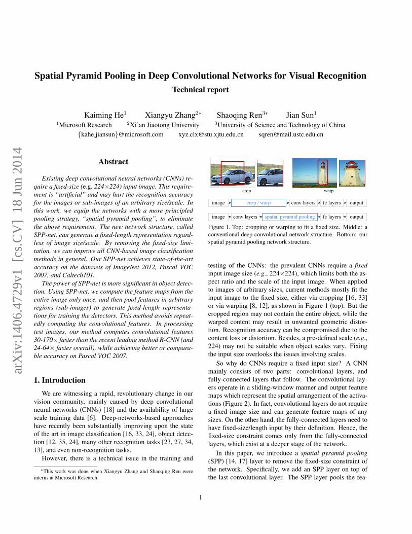
Figure 1. Top: cropping or warping to fit a fixed size. Middle: aconventional deep convolutional network structure. Bottom: ourspatial pyramid pooling network structure.

testing of the CNNs: the prevalent CNNs require a fixedinput image size (e.g., 224×224), which limits both the as-pect ratio and the scale of the input image. When appliedto images of arbitrary sizes, current methods mostly fit theinput image to the fixed size, either via cropping [16, 33]or via warping [8, 12], as shown in Figure 1 (top). But thecropped region may not contain the entire object, while thewarped content may result in unwanted geometric distor-tion. Recognition accuracy can be compromised due to thecontent loss or distortion. Besides, a pre-defined scale (e.g.,224) may not be suitable when object scales vary. Fixingthe input size overlooks the issues involving scales.

So why do CNNs require a fixed input size? A CNNmainly consists of two parts: convolutional layers, andfully-connected layers that follow. The convolutional lay-ers operate in a sliding-window manner and output featuremaps which represent the spatial arrangement of the activa-tions (Figure 2). In fact, convolutional layers do not requirea fixed image size and can generate feature maps of anysizes. On the other hand, the fully-connected layers need tohave fixed-size/length input by their definition. Hence, thefixed-size constraint comes only from the fully-connectedlayers, which exist at a deeper stage of the network.

In this paper, we introduce a spatial pyramid pooling(SPP) [14, 17] layer to remove the fixed-size constraint ofthe network. Specifically, we add an SPP layer on top ofthe last convolutional layer. The SPP layer pools the fea-

1

arX

iv:1

406.

4729

v1 [

cs.C

V]

18

Jun

2014

tures and generates fixed-length outputs, which are then fedinto the fully-connected layers (or other classifiers). In otherwords, we perform some information “aggregation” at adeeper stage of the network hierarchy (between convolu-tional layers and fully-connected layers) to avoid the needfor cropping or warping at the beginning. Figure 1 (bottom)shows the change of the network architecture by introducingthe SPP layer. We call the new network structure SPP-net.

We believe that aggregation at a deeper stage is morephysiologically sound and more compatible with the hierar-chical information processing in our brains. When an ob-ject comes into our field of view, it is more reasonable thatour brains consider it as a whole instead of cropping it intoseveral “views” at the beginning. Similarly, it is unlikelythat our brains distort all object candidates into fixed-sizeregions for detecting/locating them. It is more likely thatour brains handle arbitrarily-shaped objects at some deeperlayers, by aggregating the already deeply processed infor-mation from the previous layers.

Spatial pyramid pooling [14, 17] (popularly known asspatial pyramid matching or SPM [17]), as an extension ofthe Bag-of-Words (BoW) model [25], is one of the mostsuccessful methods in computer vision. It partitions the im-age into divisions from finer to coarser levels, and aggre-gates local features in them. SPP has long been a key com-ponent in the leading and competition-winning systems forclassification (e.g., [32, 30, 22]) and detection (e.g., [28])before the recent prevalence of CNNs. Nevertheless, SPPhas not been considered in the context of CNNs. We notethat SPP has several remarkable properties for deep CNNs:1) SPP is able to generate a fixed-length output regardless ofthe input size, while the sliding window pooling used in theprevious deep networks [16] cannot; 2) SPP uses multi-levelspatial bins, while the sliding window pooling uses only asingle window size. Multi-level pooling has been shown tobe robust to object deformations [17]; 3) SPP can pool fea-tures extracted at variable scales thanks to the flexibility ofinput scales. Through experiments we show that all thesefactors elevate the recognition accuracy of deep networks.

The flexibility of SPP-net makes it possible to generatea full-image representation for testing. Moreover, it also al-lows us to feed images with varying sizes or scales duringtraining, which increases scale-invariance and reduces therisk of over-fitting. We develop a simple multi-size trainingmethod to exploit the properties of SPP-net. Through a se-ries of controlled experiments, we demonstrate the gains ofusing multi-level pooling, full-image representations, andvariable scales. On the ImageNet 2012 dataset, our networkreduces the top-1 error by 1.8% compared to its counterpartwithout SPP. The fixed-length representations given by thispre-trained network are also used to train SVM classifierson other datasets. Our method achieves 91.4% accuracy onCaltech101 [10] and 80.1% mean Average Precision (mAP)

on Pascal VOC 2007 [9] using only a single full-image rep-resentation (single-view testing).

SPP-net shows even greater strength in object detection.In the leading object detection method R-CNN [12], the fea-tures from candidate windows are extracted via deep convo-lutional networks. This method shows remarkable detectionaccuracy on both the VOC and ImageNet datasets. But thefeature computation in R-CNN is time-consuming, becauseit repeatedly applies the deep convolutional networks to theraw pixels of thousands of warped regions per image. Inthis paper, we show that we can run the convolutional lay-ers only once on the entire image (regardless of the num-ber of windows), and then extract features by SPP-net onthe feature maps. This method yields a speedup of overone hundred times over R-CNN. Note that training/runninga detector on the feature maps (rather than image regions)is actually a more popular idea [11, 5, 28, 24]. But SPP-net inherits the power of the deep CNN feature maps andalso the flexibility of SPP on arbitrary window sizes, whichleads to outstanding accuracy and efficiency. In our exper-iment, the SPP-net-based system (built upon the R-CNNpipeline) computes convolutional features 30-170× fasterthan R-CNN, and is overall 24-64× faster, while has betteror comparable accuracy. We further propose a simple modelcombination method to achieve a new state-of-the-art result(mAP 60.9%) on the Pascal VOC 2007 detection task.

2. Deep Networks with Spatial Pyramid Pooling

2.1. Convolutional Layers and Feature Maps

Consider the popular seven-layer architectures [16, 33].The first five layers are convolutional, some of which arefollowed by pooling layers. These pooling layers can alsobe considered as “convolutional”, in the sense that they areusing sliding windows. The last two layers are fully con-nected, with an N-way softmax as the output, where N isthe number of categories.

The deep network described above needs a fixed imagesize. However, we notice the requirement of fixed sizes isonly due to the fully-connected layers that demand fixed-length vectors as inputs. On the other hand, the convo-lutional layers accept inputs of arbitrary sizes. The con-volutional layers use sliding filters, and their outputs haveroughly the same aspect ratio as the inputs. These outputsare known as feature maps [18] - they involve not only thestrength of the responses, but also their spatial positions.

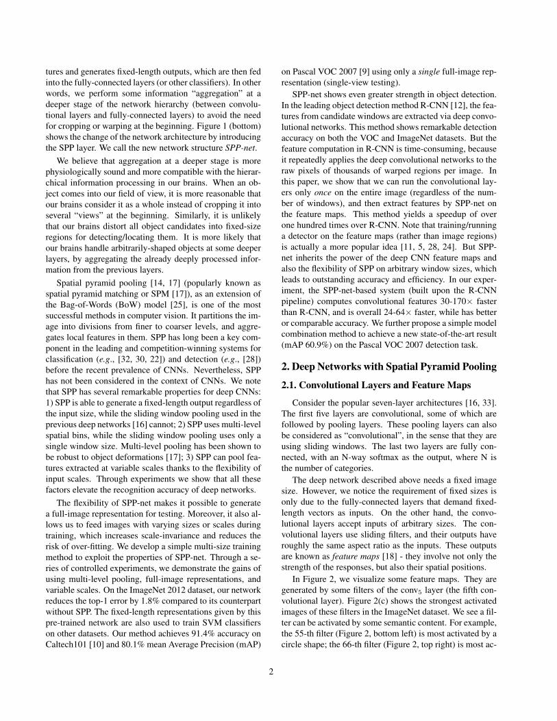
In Figure 2, we visualize some feature maps. They aregenerated by some filters of the conv5 layer (the fifth con-volutional layer). Figure 2(c) shows the strongest activatedimages of these filters in the ImageNet dataset. We see a fil-ter can be activated by some semantic content. For example,the 55-th filter (Figure 2, bottom left) is most activated by acircle shape; the 66-th filter (Figure 2, top right) is most ac-

2

filter #175

filter #55

(a) image (b) feature maps (c) strongest activations

filter #66

filter #118

(a) image (b) feature maps (c) strongest activations

Figure 2. Visualization of the feature maps. (a) Two images in Pascal VOC 2007. (b) The feature maps of some conv5 filters. The arrowsindicate the strongest responses and their corresponding positions in the images. (c) The ImageNet images that have the strongest responsesof the corresponding filters. The green rectangles mark the receptive fields of the strongest responses.

tivated by a ∧-shape; and the 118-th filter (Figure 2, bottomright) is most activated by a ∨-shape. These shapes in theinput images (Figure 2(a)) activate the feature maps at thecorresponding positions (the arrows in Figure 2).

It is worth noticing that we generate the feature mapsin Figure 2 without fixing the input size. These featuremaps generated by deep convolutional layers are analogousto the feature maps in traditional methods [2, 4]. In thosemethods, SIFT vectors [2] or image patches [4] are denselyextracted and then encoded, e.g., by vector quantization[25, 17, 29], sparse coding [32, 30], or Fisher kernels [22].These encoded features consist of the feature maps, and arethen pooled by Bag-of-Words (BoW) [25] or spatial pyra-mids [14, 17]. Analogously, the deep convolutional featurescan be pooled in a similar way.

2.2. The Spatial Pyramid Pooling Layer

The convolutional layers accept arbitrary input sizes,but they produce outputs of variable sizes. The classifiers(SVM/softmax) or fully-connected layers require fixed-length vectors. Such vectors can be generated by the Bag-of-Words (BoW) approach [25] that pools the features to-gether. Spatial pyramid pooling [14, 17] improves BoW inthat it can maintain spatial information by pooling in localspatial bins. These spatial bins have sizes proportional tothe image size, so the number of bins is fixed regardlessof the image size. This is in contrast to the sliding win-dow pooling of the previous deep networks [16], where thenumber of sliding windows depends on the input size.

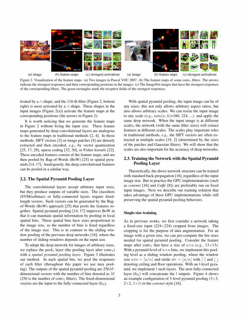
To adopt the deep network for images of arbitrary sizes,we replace the pool5 layer (the pooling layer after conv5)with a spatial pyramid pooling layer. Figure 3 illustratesour method. In each spatial bin, we pool the responsesof each filter (throughout this paper we use max pool-ing). The outputs of the spatial pyramid pooling are 256M -dimensional vectors with the number of bins denoted as M(256 is the number of conv5 filters). The fixed-dimensionalvectors are the input to the fully-connected layer (fc6).

With spatial pyramid pooling, the input image can be ofany sizes; this not only allows arbitrary aspect ratios, butalso allows arbitrary scales. We can resize the input imageto any scale (e.g., min(w, h)=180, 224, ...) and apply thesame deep network. When the input image is at differentscales, the network (with the same filter sizes) will extractfeatures at different scales. The scales play important rolesin traditional methods, e.g., the SIFT vectors are often ex-tracted at multiple scales [19, 2] (determined by the sizesof the patches and Gaussian filters). We will show that thescales are also important for the accuracy of deep networks.

2.3. Training the Network with the Spatial PyramidPooling Layer

Theoretically, the above network structure can be trainedwith standard back-propagation [18], regardless of the inputimage size. But in practice the GPU implementations (suchas convnet [16] and Caffe [8]) are preferably run on fixedinput images. Next we describe our training solution thattakes advantage of these GPU implementations while stillpreserving the spatial pyramid pooling behaviors.

Single-size training

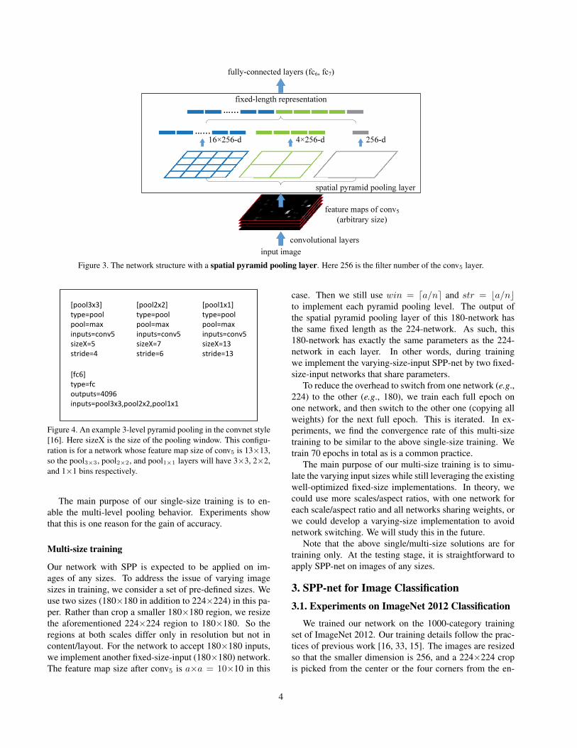
As in previous works, we first consider a network takinga fixed-size input (224×224) cropped from images. Thecropping is for the purpose of data augmentation. For animage with a given size, we can pre-compute the bin sizesneeded for spatial pyramid pooling. Consider the featuremaps after conv5 that have a size of a×a (e.g., 13×13).With a pyramid level of n×n bins, we implement this pool-ing level as a sliding window pooling, where the windowsize win = da/ne and stride str = ba/nc with d·e and b·cdenoting ceiling and floor operations. With an l-level pyra-mid, we implement l such layers. The next fully-connectedlayer (fc6) will concatenate the l outputs. Figure 4 showsan example configuration of 3-level pyramid pooling (3×3,2×2, 1×1) in the convnet style [16].

3

convolutional layers

feature maps of conv5

(arbitrary size)

fixed-length representation

input image

16×256-d 4×256-d 256-d

…...

…...

spatial pyramid pooling layer

fully-connected layers (fc6, fc7)

Figure 3. The network structure with a spatial pyramid pooling layer. Here 256 is the filter number of the conv5 layer.

[fc6]

type=fc

outputs=4096

inputs=pool3x3,pool2x2,pool1x1

[pool1x1]

type=pool

pool=max

inputs=conv5

sizeX=13

stride=13

[pool3x3]

type=pool

pool=max

inputs=conv5

sizeX=5

stride=4

[pool2x2]

type=pool

pool=max

inputs=conv5

sizeX=7

stride=6

Figure 4. An example 3-level pyramid pooling in the convnet style[16]. Here sizeX is the size of the pooling window. This configu-ration is for a network whose feature map size of conv5 is 13×13,so the pool3×3, pool2×2, and pool1×1 layers will have 3×3, 2×2,and 1×1 bins respectively.

The main purpose of our single-size training is to en-able the multi-level pooling behavior. Experiments showthat this is one reason for the gain of accuracy.

Multi-size training

Our network with SPP is expected to be applied on im-ages of any sizes. To address the issue of varying imagesizes in training, we consider a set of pre-defined sizes. Weuse two sizes (180×180 in addition to 224×224) in this pa-per. Rather than crop a smaller 180×180 region, we resizethe aforementioned 224×224 region to 180×180. So theregions at both scales differ only in resolution but not incontent/layout. For the network to accept 180×180 inputs,we implement another fixed-size-input (180×180) network.The feature map size after conv5 is a×a = 10×10 in this

case. Then we still use win = da/ne and str = ba/ncto implement each pyramid pooling level. The output ofthe spatial pyramid pooling layer of this 180-network hasthe same fixed length as the 224-network. As such, this180-network has exactly the same parameters as the 224-network in each layer. In other words, during trainingwe implement the varying-size-input SPP-net by two fixed-size-input networks that share parameters.

To reduce the overhead to switch from one network (e.g.,224) to the other (e.g., 180), we train each full epoch onone network, and then switch to the other one (copying allweights) for the next full epoch. This is iterated. In ex-periments, we find the convergence rate of this multi-sizetraining to be similar to the above single-size training. Wetrain 70 epochs in total as is a common practice.

The main purpose of our multi-size training is to simu-late the varying input sizes while still leveraging the existingwell-optimized fixed-size implementations. In theory, wecould use more scales/aspect ratios, with one network foreach scale/aspect ratio and all networks sharing weights, orwe could develop a varying-size implementation to avoidnetwork switching. We will study this in the future.

Note that the above single/multi-size solutions are fortraining only. At the testing stage, it is straightforward toapply SPP-net on images of any sizes.

3. SPP-net for Image Classification3.1. Experiments on ImageNet 2012 Classification

We trained our network on the 1000-category trainingset of ImageNet 2012. Our training details follow the prac-tices of previous work [16, 33, 15]. The images are resizedso that the smaller dimension is 256, and a 224×224 cropis picked from the center or the four corners from the en-

4

method test scale test views top-1 val top-5 val(a) Krizhevsky et al. [16] 1 10 40.7 18.2

(b1) Overfeat (fast) [24] 1 - 39.01 16.97(b2) Overfeat (fast) [24] 6 - 38.12 16.27(b3) Overfeat (big) [24] 4 - 35.74 14.18(c1) Howard (base) [15] 3 162 37.0 15.8(c2) Howard (high-res) [15] 3 162 36.8 16.2(d1) Zeiler & Fergus (ZF) (fast) [33] 1 10 38.4 16.5(d2) Zeiler & Fergus (ZF) (big) [33] 1 10 37.5 16.0(e1) our impl of ZF (fast) 1 10 35.99 14.76(e2) SPP-net4, single-size trained 1 10 35.06 14.04(e3) SPP-net6, single-size trained 1 10 34.98 14.14(e4) SPP-net6, multi-size trained 1 10 34.60 13.64(e5) SPP-net6, multi-size trained 1 8+2full 34.16 13.57

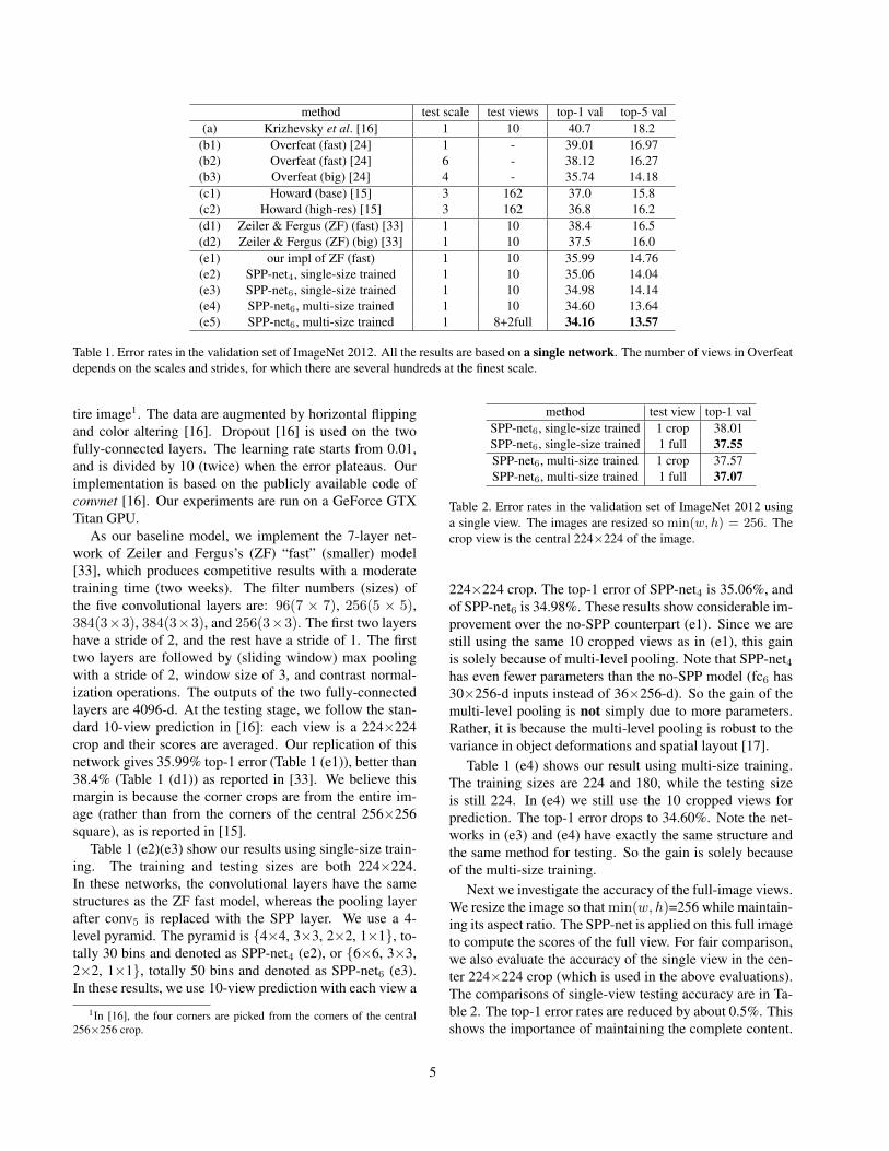
Table 1. Error rates in the validation set of ImageNet 2012. All the results are based on a single network. The number of views in Overfeatdepends on the scales and strides, for which there are several hundreds at the finest scale.

tire image1. The data are augmented by horizontal flippingand color altering [16]. Dropout [16] is used on the twofully-connected layers. The learning rate starts from 0.01,and is divided by 10 (twice) when the error plateaus. Ourimplementation is based on the publicly available code ofconvnet [16]. Our experiments are run on a GeForce GTXTitan GPU.

As our baseline model, we implement the 7-layer net-work of Zeiler and Fergus’s (ZF) “fast” (smaller) model[33], which produces competitive results with a moderatetraining time (two weeks). The filter numbers (sizes) ofthe five convolutional layers are: 96(7 × 7), 256(5 × 5),384(3×3), 384(3×3), and 256(3×3). The first two layershave a stride of 2, and the rest have a stride of 1. The firsttwo layers are followed by (sliding window) max poolingwith a stride of 2, window size of 3, and contrast normal-ization operations. The outputs of the two fully-connectedlayers are 4096-d. At the testing stage, we follow the stan-dard 10-view prediction in [16]: each view is a 224×224crop and their scores are averaged. Our replication of thisnetwork gives 35.99% top-1 error (Table 1 (e1)), better than38.4% (Table 1 (d1)) as reported in [33]. We believe thismargin is because the corner crops are from the entire im-age (rather than from the corners of the central 256×256square), as is reported in [15].

Table 1 (e2)(e3) show our results using single-size train-ing. The training and testing sizes are both 224×224.In these networks, the convolutional layers have the samestructures as the ZF fast model, whereas the pooling layerafter conv5 is replaced with the SPP layer. We use a 4-level pyramid. The pyramid is {4×4, 3×3, 2×2, 1×1}, to-tally 30 bins and denoted as SPP-net4 (e2), or {6×6, 3×3,2×2, 1×1}, totally 50 bins and denoted as SPP-net6 (e3).In these results, we use 10-view prediction with each view a

1In [16], the four corners are picked from the corners of the central256×256 crop.

method test view top-1 valSPP-net6, single-size trained 1 crop 38.01SPP-net6, single-size trained 1 full 37.55SPP-net6, multi-size trained 1 crop 37.57SPP-net6, multi-size trained 1 full 37.07

Table 2. Error rates in the validation set of ImageNet 2012 usinga single view. The images are resized so min(w, h) = 256. Thecrop view is the central 224×224 of the image.

224×224 crop. The top-1 error of SPP-net4 is 35.06%, andof SPP-net6 is 34.98%. These results show considerable im-provement over the no-SPP counterpart (e1). Since we arestill using the same 10 cropped views as in (e1), this gainis solely because of multi-level pooling. Note that SPP-net4has even fewer parameters than the no-SPP model (fc6 has30×256-d inputs instead of 36×256-d). So the gain of themulti-level pooling is not simply due to more parameters.Rather, it is because the multi-level pooling is robust to thevariance in object deformations and spatial layout [17].

Table 1 (e4) shows our result using multi-size training.The training sizes are 224 and 180, while the testing sizeis still 224. In (e4) we still use the 10 cropped views forprediction. The top-1 error drops to 34.60%. Note the net-works in (e3) and (e4) have exactly the same structure andthe same method for testing. So the gain is solely becauseof the multi-size training.

Next we investigate the accuracy of the full-image views.We resize the image so that min(w, h)=256 while maintain-ing its aspect ratio. The SPP-net is applied on this full imageto compute the scores of the full view. For fair comparison,we also evaluate the accuracy of the single view in the cen-ter 224×224 crop (which is used in the above evaluations).The comparisons of single-view testing accuracy are in Ta-ble 2. The top-1 error rates are reduced by about 0.5%. Thisshows the importance of maintaining the complete content.

5

(a) (b) (c) (d)model plain net SPP-net SPP-net SPP-net

crop crop full fullsize 224×224 224×224 224×- 392×-

conv4 59.96 57.28 - -conv5 66.34 65.43 - -

pool5 (6×6) 69.14 68.76 70.82 71.67fc6 74.86 75.55 77.32 78.78fc7 75.90 76.45 78.39 80.10

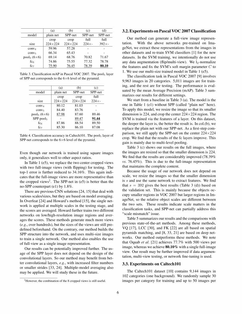
Table 3. Classification mAP in Pascal VOC 2007. The pool5 layerof SPP-net corresponds to the 6×6 level of the pyramid.

(a) (b) (c)model plain net SPP-net SPP-net

crop crop fullsize 224×224 224×224 224×-

conv4 80.12 81.03 -conv5 84.40 83.76 -

pool5 (6×6) 87.98 87.60 89.46SPP pool5 - 89.47 91.44

fc6 87.86 88.54 89.50fc7 85.30 86.10 87.08

Table 4. Classification accuracy in Caltech101. The pool5 layer ofSPP-net corresponds to the 6×6 level of the pyramid.

Even though our network is trained using square imagesonly, it generalizes well to other aspect ratios.

In Table 1 (e5), we replace the two center cropped viewswith two full-image views (with flipping) for testing. Thetop-1 error is further reduced to 34.16%. This again indi-cates that the full-image views are more representative thanthe cropped views2. The SPP-net in (e5) is better than theno-SPP counterpart (e1) by 1.8%.

There are previous CNN solutions [24, 15] that deal withvarious scales/sizes, but they are based on model averaging.In Overfeat [24] and Howard’s method [15], the single net-work is applied at multiple scales in the testing stage, andthe scores are averaged. Howard further trains two differentnetworks on low/high-resolution image regions and aver-ages the scores. These methods generate much more views(e.g., over hundreds), but the sizes of the views are still pre-defined beforehand. On the contrary, our method builds theSPP structure into the network, and uses multi-size imagesto train a single network. Our method also enables the useof full-view as a single image representation.

Our results can be potentially improved further. The us-age of the SPP layer does not depend on the design of theconvolutional layers. So our method may benefit from bet-ter convolutional layers, e.g., with increased filter numbersor smaller strides [33, 24]. Multiple-model averaging alsomay be applied. We will study these in the future.

2However, the combination of the 8 cropped views is still useful.

3.2. Experiments on Pascal VOC 2007 Classification

Our method can generate a full-view image represen-tation. With the above networks pre-trained on Ima-geNet, we extract these representations from the images inother datasets and re-train SVM classifiers [1] for the newdatasets. In the SVM training, we intentionally do not useany data augmentation (flip/multi-view). We l2-normalizethe features and fix the SVM’s soft margin parameter C to1. We use our multi-size trained model in Table 1 (e5).

The classification task in Pascal VOC 2007 [9] involves9,963 images in 20 categories. 5,011 images are for train-ing, and the rest are for testing. The performance is eval-uated by the mean Average Precision (mAP). Table 3 sum-marizes our results for different settings.

We start from a baseline in Table 3 (a). The model is theone in Table 1 (e1) without SPP (called “plain net” here).To apply this model, we resize the image so that its smallerdimension is 224, and crop the center 224×224 region. TheSVM is trained via the features of a layer. On this dataset,the deeper the layer is, the better the result is. In col.(b), wereplace the plain net with our SPP-net. As a first-step com-parison, we still apply the SPP-net on the center 224×224crop. We find that the results of the fc layers improve. Thisgain is mainly due to multi-level pooling.

Table 3 (c) shows our results on the full images, wherethe images are resized so that the smaller dimension is 224.We find that the results are considerably improved (78.39%vs. 76.45%). This is due to the full-image representationthat maintains the complete content.

Because the usage of our network does not depend onscale, we resize the images so that the smaller dimensionis s and use the same network to extract features. We findthat s = 392 gives the best results (Table 3 (d)) based onthe validation set. This is mainly because the objects oc-cupy smaller regions in VOC 2007 but larger regions in Im-ageNet, so the relative object scales are different betweenthe two sets. These results indicate scale matters in theclassification tasks, and SPP-net can partially address this“scale mismatch” issue.

Table 5 summarizes our results and the comparisons withprevious state-of-the-art methods. Among these methods,VQ [17], LCC [30], and FK [22] are all based on spatialpyramids matching, and [8, 33, 21] are based on deep net-works. Our method outperforms these methods. We notethat Oquab et al. [21] achieves 77.7% with 500 views perimage, whereas we achieve 80.10% with a single full-imageview. Our result may be further improved if data argumen-tation, multi-view testing, or network fine-tuning is used.

3.3. Experiments on Caltech101

The Caltech101 dataset [10] contains 9,144 images in102 categories (one background). We randomly sample 30images per category for training and up to 50 images per

6

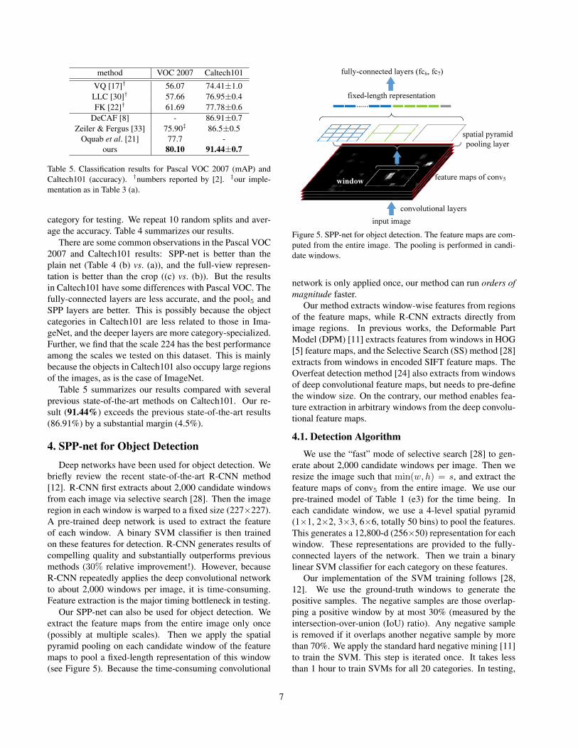
method VOC 2007 Caltech101

VQ [17]† 56.07 74.41±1.0LLC [30]† 57.66 76.95±0.4FK [22]† 61.69 77.78±0.6

DeCAF [8] - 86.91±0.7Zeiler & Fergus [33] 75.90‡ 86.5±0.5

Oquab et al. [21] 77.7 -ours 80.10 91.44±0.7

Table 5. Classification results for Pascal VOC 2007 (mAP) andCaltech101 (accuracy). †numbers reported by [2]. ‡our imple-mentation as in Table 3 (a).

category for testing. We repeat 10 random splits and aver-age the accuracy. Table 4 summarizes our results.

There are some common observations in the Pascal VOC2007 and Caltech101 results: SPP-net is better than theplain net (Table 4 (b) vs. (a)), and the full-view represen-tation is better than the crop ((c) vs. (b)). But the resultsin Caltech101 have some differences with Pascal VOC. Thefully-connected layers are less accurate, and the pool5 andSPP layers are better. This is possibly because the objectcategories in Caltech101 are less related to those in Ima-geNet, and the deeper layers are more category-specialized.Further, we find that the scale 224 has the best performanceamong the scales we tested on this dataset. This is mainlybecause the objects in Caltech101 also occupy large regionsof the images, as is the case of ImageNet.

Table 5 summarizes our results compared with severalprevious state-of-the-art methods on Caltech101. Our re-sult (91.44%) exceeds the previous state-of-the-art results(86.91%) by a substantial margin (4.5%).

4. SPP-net for Object DetectionDeep networks have been used for object detection. We

briefly review the recent state-of-the-art R-CNN method[12]. R-CNN first extracts about 2,000 candidate windowsfrom each image via selective search [28]. Then the imageregion in each window is warped to a fixed size (227×227).A pre-trained deep network is used to extract the featureof each window. A binary SVM classifier is then trainedon these features for detection. R-CNN generates results ofcompelling quality and substantially outperforms previousmethods (30% relative improvement!). However, becauseR-CNN repeatedly applies the deep convolutional networkto about 2,000 windows per image, it is time-consuming.Feature extraction is the major timing bottleneck in testing.

Our SPP-net can also be used for object detection. Weextract the feature maps from the entire image only once(possibly at multiple scales). Then we apply the spatialpyramid pooling on each candidate window of the featuremaps to pool a fixed-length representation of this window(see Figure 5). Because the time-consuming convolutional

spatial pyramid

pooling layer

feature maps of conv5

convolutional layers

fixed-length representation

input image

window

…...

fully-connected layers (fc6, fc7)

Figure 5. SPP-net for object detection. The feature maps are com-puted from the entire image. The pooling is performed in candi-date windows.

network is only applied once, our method can run orders ofmagnitude faster.

Our method extracts window-wise features from regionsof the feature maps, while R-CNN extracts directly fromimage regions. In previous works, the Deformable PartModel (DPM) [11] extracts features from windows in HOG[5] feature maps, and the Selective Search (SS) method [28]extracts from windows in encoded SIFT feature maps. TheOverfeat detection method [24] also extracts from windowsof deep convolutional feature maps, but needs to pre-definethe window size. On the contrary, our method enables fea-ture extraction in arbitrary windows from the deep convolu-tional feature maps.

4.1. Detection Algorithm

We use the “fast” mode of selective search [28] to gen-erate about 2,000 candidate windows per image. Then weresize the image such that min(w, h) = s, and extract thefeature maps of conv5 from the entire image. We use ourpre-trained model of Table 1 (e3) for the time being. Ineach candidate window, we use a 4-level spatial pyramid(1×1, 2×2, 3×3, 6×6, totally 50 bins) to pool the features.This generates a 12,800-d (256×50) representation for eachwindow. These representations are provided to the fully-connected layers of the network. Then we train a binarylinear SVM classifier for each category on these features.

Our implementation of the SVM training follows [28,12]. We use the ground-truth windows to generate thepositive samples. The negative samples are those overlap-ping a positive window by at most 30% (measured by theintersection-over-union (IoU) ratio). Any negative sampleis removed if it overlaps another negative sample by morethan 70%. We apply the standard hard negative mining [11]to train the SVM. This step is iterated once. It takes lessthan 1 hour to train SVMs for all 20 categories. In testing,

7

the classifier is used to score the candidate windows. Thenwe use non-maximum suppression [11] (threshold of 30%)on the scored windows.

Our method can be improved by multi-scale feature ex-traction. We resize the image such that min(w, h) =s ∈ {480, 576, 688, 864, 1200}, and compute the featuremaps of conv5 for each scale. One strategy of combiningthe features from these scales is to pool them channel-by-channel. But we empirically find that another strategy pro-vides better results. For each candidate window, we choosea single scale s ∈ {480, 576, 688, 864, 1200} such that thescaled candidate window has a number of pixels closest to224×224. Then we only use the feature maps extractedfrom this scale to compute the feature of this window. Ifthe pre-defined scales are dense enough and the window isapproximately square, our method is roughly equivalent toresizing the window to 224×224 and then extracting fea-tures from it. Nevertheless, our method only requires com-puting the feature maps once (at each scale) from the entireimage, regardless of the number of candidate windows.

We also fine-tune our pre-trained network, following[12]. Since our features are pooled from the conv5 featuremaps from windows of any sizes, for simplicity we onlyfine-tune the fully-connected layers. In this case, the datalayer accepts the fixed-length pooled features after conv5,and the fc6,7 layers and a new 21-way (one extra negativecategory) fc8 layer follow. The fc8 weights are initializedwith a Gaussian distribution of σ=0.01. We fix all the learn-ing rates to 1e-4 and then adjust to 1e-5 for all three layers.During fine-tuning, the positive samples are those overlap-ping with a ground-truth window by [0.5, 1], and the nega-tive samples by [0.1, 0.5). In each mini-batch, 25% of thesamples are positive. We train 250k mini-batches using thelearning rate 1e-4, and then 50k mini-batches using 1e-5.Because we only fine-tune the fully-connected layers, thetraining is very fast and takes about 2 hours on the GPU.Also following [12], we use bounding box regression topost-process the prediction windows. The features used forregression are the pooled features from conv5 (as a coun-terpart of the pool5 features used in [12]). The windowsused for the regression training are those overlapping witha ground-truth window by at least 50%.

We will release the code of our algorithm to facilitatereproduction of the results3.

4.2. Detection Results

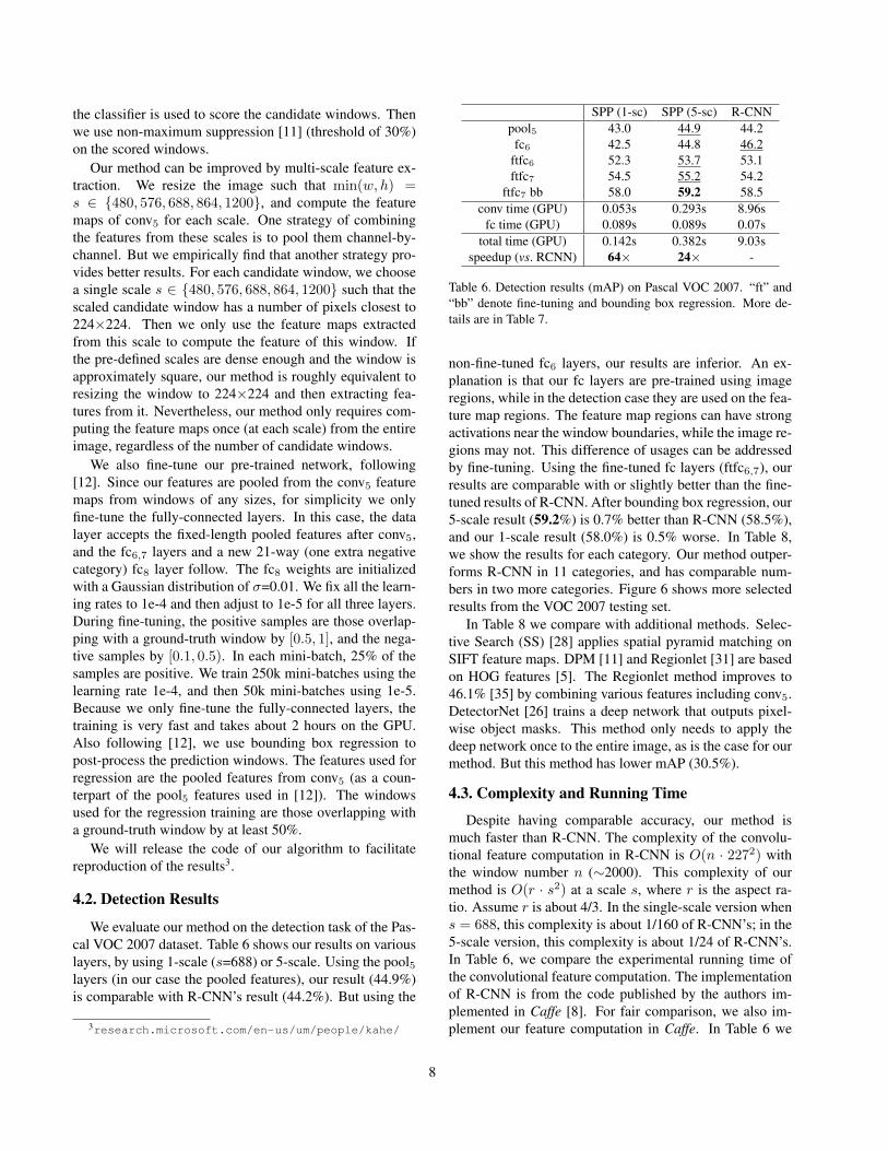
We evaluate our method on the detection task of the Pas-cal VOC 2007 dataset. Table 6 shows our results on variouslayers, by using 1-scale (s=688) or 5-scale. Using the pool5layers (in our case the pooled features), our result (44.9%)is comparable with R-CNN’s result (44.2%). But using the

3research.microsoft.com/en-us/um/people/kahe/

SPP (1-sc) SPP (5-sc) R-CNNpool5 43.0 44.9 44.2

fc6 42.5 44.8 46.2ftfc6 52.3 53.7 53.1ftfc7 54.5 55.2 54.2

ftfc7 bb 58.0 59.2 58.5conv time (GPU) 0.053s 0.293s 8.96s

fc time (GPU) 0.089s 0.089s 0.07stotal time (GPU) 0.142s 0.382s 9.03s

speedup (vs. RCNN) 64× 24× -

Table 6. Detection results (mAP) on Pascal VOC 2007. “ft” and“bb” denote fine-tuning and bounding box regression. More de-tails are in Table 7.

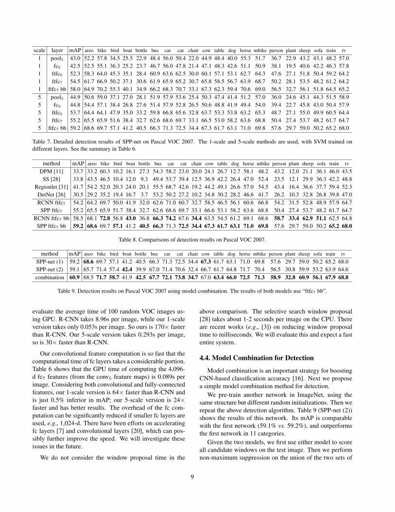
non-fine-tuned fc6 layers, our results are inferior. An ex-planation is that our fc layers are pre-trained using imageregions, while in the detection case they are used on the fea-ture map regions. The feature map regions can have strongactivations near the window boundaries, while the image re-gions may not. This difference of usages can be addressedby fine-tuning. Using the fine-tuned fc layers (ftfc6,7), ourresults are comparable with or slightly better than the fine-tuned results of R-CNN. After bounding box regression, our5-scale result (59.2%) is 0.7% better than R-CNN (58.5%),and our 1-scale result (58.0%) is 0.5% worse. In Table 8,we show the results for each category. Our method outper-forms R-CNN in 11 categories, and has comparable num-bers in two more categories. Figure 6 shows more selectedresults from the VOC 2007 testing set.

In Table 8 we compare with additional methods. Selec-tive Search (SS) [28] applies spatial pyramid matching onSIFT feature maps. DPM [11] and Regionlet [31] are basedon HOG features [5]. The Regionlet method improves to46.1% [35] by combining various features including conv5.DetectorNet [26] trains a deep network that outputs pixel-wise object masks. This method only needs to apply thedeep network once to the entire image, as is the case for ourmethod. But this method has lower mAP (30.5%).

4.3. Complexity and Running Time

Despite having comparable accuracy, our method ismuch faster than R-CNN. The complexity of the convolu-tional feature computation in R-CNN is O(n · 2272) withthe window number n (∼2000). This complexity of ourmethod is O(r · s2) at a scale s, where r is the aspect ra-tio. Assume r is about 4/3. In the single-scale version whens = 688, this complexity is about 1/160 of R-CNN’s; in the5-scale version, this complexity is about 1/24 of R-CNN’s.In Table 6, we compare the experimental running time ofthe convolutional feature computation. The implementationof R-CNN is from the code published by the authors im-plemented in Caffe [8]. For fair comparison, we also im-plement our feature computation in Caffe. In Table 6 we

8

scale layer mAP areo bike bird boat bottle bus car cat chair cow table dog horse mbike person plant sheep sofa train tv

1 pool5 43.0 52.2 57.8 34.5 25.5 22.9 48.4 56.0 50.4 22.0 44.9 48.4 40.0 55.3 51.7 36.7 22.9 43.2 43.1 48.2 57.01 fc6 42.5 52.5 55.1 36.3 25.2 23.7 46.7 56.0 47.8 21.4 47.1 48.3 42.6 51.1 50.9 38.1 19.5 40.6 42.2 46.3 57.81 ftfc6 52.3 58.3 64.0 45.3 35.1 28.4 60.9 63.6 62.5 30.0 60.1 57.1 53.1 62.7 64.3 47.6 27.1 51.8 50.4 59.2 64.21 ftfc7 54.5 61.7 66.9 50.2 37.1 30.6 61.9 65.9 65.2 30.7 65.8 58.5 56.7 63.9 68.7 50.2 28.1 53.5 48.2 61.2 64.21 ftfc7 bb 58.0 64.9 70.2 55.3 40.1 34.9 66.2 68.3 70.7 33.1 67.3 62.3 59.4 70.6 69.0 56.5 32.7 56.1 51.8 64.5 65.25 pool5 44.9 50.6 59.0 37.1 27.0 28.1 51.9 57.9 53.6 25.4 50.3 47.4 41.4 51.2 57.0 36.0 24.6 45.1 44.3 51.5 58.95 fc6 44.8 54.4 57.1 38.4 26.8 27.6 51.4 57.9 52.8 26.5 50.6 48.8 41.9 49.4 54.0 39.4 22.7 45.8 43.0 50.4 57.95 ftfc6 53.7 64.4 64.1 47.9 35.0 33.2 59.8 66.8 65.6 32.8 63.7 53.3 53.8 63.2 65.3 48.7 27.1 55.0 49.9 60.5 64.45 ftfc7 55.2 65.5 65.9 51.6 38.4 32.7 62.6 68.6 69.7 33.1 66.5 53.0 58.2 63.6 68.8 50.4 27.4 53.7 48.2 61.7 64.75 ftfc7 bb 59.2 68.6 69.7 57.1 41.2 40.5 66.3 71.3 72.5 34.4 67.3 61.7 63.1 71.0 69.8 57.6 29.7 59.0 50.2 65.2 68.0

Table 7. Detailed detection results of SPP-net on Pascal VOC 2007. The 1-scale and 5-scale methods are used, with SVM trained ondifferent layers. See the summary in Table 6.

method mAP areo bike bird boat bottle bus car cat chair cow table dog horse mbike person plant sheep sofa train tv

DPM [11] 33.7 33.2 60.3 10.2 16.1 27.3 54.3 58.2 23.0 20.0 24.1 26.7 12.7 58.1 48.2 43.2 12.0 21.1 36.1 46.0 43.5SS [28] 33.8 43.5 46.5 10.4 12.0 9.3 49.4 53.7 39.4 12.5 36.9 42.2 26.4 47.0 52.4 23.5 12.1 29.9 36.3 42.2 48.8

Regionlet [31] 41.7 54.2 52.0 20.3 24.0 20.1 55.5 68.7 42.6 19.2 44.2 49.1 26.6 57.0 54.5 43.4 16.4 36.6 37.7 59.4 52.3DetNet [26] 30.5 29.2 35.2 19.4 16.7 3.7 53.2 50.2 27.2 10.2 34.8 30.2 28.2 46.6 41.7 26.2 10.3 32.8 26.8 39.8 47.0RCNN ftfc7 54.2 64.2 69.7 50.0 41.9 32.0 62.6 71.0 60.7 32.7 58.5 46.5 56.1 60.6 66.8 54.2 31.5 52.8 48.9 57.9 64.7

SPP ftfc7 55.2 65.5 65.9 51.7 38.4 32.7 62.6 68.6 69.7 33.1 66.6 53.1 58.2 63.6 68.8 50.4 27.4 53.7 48.2 61.7 64.7RCNN ftfc7 bb 58.5 68.1 72.8 56.8 43.0 36.8 66.3 74.2 67.6 34.4 63.5 54.5 61.2 69.1 68.6 58.7 33.4 62.9 51.1 62.5 64.8

SPP ftfc7 bb 59.2 68.6 69.7 57.1 41.2 40.5 66.3 71.3 72.5 34.4 67.3 61.7 63.1 71.0 69.8 57.6 29.7 59.0 50.2 65.2 68.0

Table 8. Comparisons of detection results on Pascal VOC 2007.

method mAP areo bike bird boat bottle bus car cat chair cow table dog horse mbike person plant sheep sofa train tv

SPP-net (1) 59.2 68.6 69.7 57.1 41.2 40.5 66.3 71.3 72.5 34.4 67.3 61.7 63.1 71.0 69.8 57.6 29.7 59.0 50.2 65.2 68.0SPP-net (2) 59.1 65.7 71.4 57.4 42.4 39.9 67.0 71.4 70.6 32.4 66.7 61.7 64.8 71.7 70.4 56.5 30.8 59.9 53.2 63.9 64.6combination 60.9 68.5 71.7 58.7 41.9 42.5 67.7 72.1 73.8 34.7 67.0 63.4 66.0 72.5 71.3 58.9 32.8 60.9 56.1 67.9 68.8

Table 9. Detection results on Pascal VOC 2007 using model combination. The results of both models use “ftfc7 bb”.

evaluate the average time of 100 random VOC images us-ing GPU. R-CNN takes 8.96s per image, while our 1-scaleversion takes only 0.053s per image. So ours is 170× fasterthan R-CNN. Our 5-scale version takes 0.293s per image,so is 30× faster than R-CNN.

Our convolutional feature computation is so fast that thecomputational time of fc layers takes a considerable portion.Table 6 shows that the GPU time of computing the 4,096-d fc7 features (from the conv5 feature maps) is 0.089s perimage. Considering both convolutional and fully-connectedfeatures, our 1-scale version is 64× faster than R-CNN andis just 0.5% inferior in mAP; our 5-scale version is 24×faster and has better results. The overhead of the fc com-putation can be significantly reduced if smaller fc layers areused, e.g., 1,024-d. There have been efforts on acceleratingfc layers [7] and convolutional layers [20], which can pos-sibly further improve the speed. We will investigate theseissues in the future.

We do not consider the window proposal time in the

above comparison. The selective search window proposal[28] takes about 1-2 seconds per image on the CPU. Thereare recent works (e.g., [3]) on reducing window proposaltime to milliseconds. We will evaluate this and expect a fastentire system.

4.4. Model Combination for Detection

Model combination is an important strategy for boostingCNN-based classification accuracy [16]. Next we proposea simple model combination method for detection.

We pre-train another network in ImageNet, using thesame structure but different random initializations. Then werepeat the above detection algorithm. Table 9 (SPP-net (2))shows the results of this network. Its mAP is comparablewith the first network (59.1% vs. 59.2%), and outperformsthe first network in 11 categories.

Given the two models, we first use either model to scoreall candidate windows on the test image. Then we performnon-maximum suppression on the union of the two sets of

9

candidate windows (with their scores). A more confidentwindow given by one method can suppress those less con-fident given by the other method. After combination, themAP is boosted to 60.9% (Table 9). In 17 out of all 20categories the combination performs better than either indi-vidual model. This indicates that the two models are com-plementary.

We further find that the complementarity is mainly be-cause of the convolutional layers. We have tried to combinetwo randomly initialized fine-tuned results of the same con-volutional model, and found no gain.

5. ConclusionSPP is a flexible solution for handling different scales,

sizes, and aspect ratios. These issues are important in visualrecognition, but received little consideration in the contextof deep networks. We have suggested a solution to traina deep network with a spatial pyramid pooling layer. Theresulting SPP-net shows outstanding accuracy in classifica-tion/detection tasks and greatly accelerates DNN-based de-tection. Our studies also show that many time-proven tech-niques/insights in computer vision can still play importantroles in deep-networks-based recognition.

References[1] C.-C. Chang and C.-J. Lin. Libsvm: a library for support

vector machines. ACM Transactions on Intelligent Systemsand Technology (TIST), 2011.

[2] K. Chatfield, V. Lempitsky, A. Vedaldi, and A. Zisserman.The devil is in the details: an evaluation of recent featureencoding methods. In BMVC, 2011.

[3] M.-M. Cheng, Z. Zhang, W.-Y. Lin, and P. Torr. BING: Bina-rized normed gradients for objectness estimation at 300fps.In CVPR, 2014.

[4] A. Coates and A. Ng. The importance of encoding ver-sus training with sparse coding and vector quantization. InICML, 2011.

[5] N. Dalal and B. Triggs. Histograms of oriented gradients forhuman detection. In CVPR, 2005.

[6] J. Deng, W. Dong, R. Socher, L.-J. Li, K. Li, and L. Fei-Fei. Imagenet: A large-scale hierarchical image database. InCVPR, 2009.

[7] E. Denton, W. Zaremba, J. Bruna, Y. LeCun, and R. Fergus.Exploiting linear structure within convolutional networks forefficient evaluation. arXiv:1404.0736, 2014.

[8] J. Donahue, Y. Jia, O. Vinyals, J. Hoffman, N. Zhang,E. Tzeng, and T. Darrell. Decaf: A deep convolu-tional activation feature for generic visual recognition.arXiv:1310.1531, 2013.

[9] M. Everingham, L. Van Gool, C. K. I. Williams, J. Winn, andA. Zisserman. The PASCAL Visual Object Classes Chal-lenge 2007 (VOC2007) Results, 2007.

[10] L. Fei-Fei, R. Fergus, and P. Perona. Learning generativevisual models from few training examples: An incremental

bayesian approach tested on 101 object categories. CVIU,2007.

[11] P. F. Felzenszwalb, R. B. Girshick, D. McAllester, and D. Ra-manan. Object detection with discriminatively trained part-based models. PAMI, 2010.

[12] R. Girshick, J. Donahue, T. Darrell, and J. Malik. Rich fea-ture hierarchies for accurate object detection and semanticsegmentation. In CVPR, 2014.

[13] Y. Gong, L. Wang, R. Guo, and S. Lazebnik. Multi-scaleorderless pooling of deep convolutional activation features.In ArXiv:1403.1840, 2014.

[14] K. Grauman and T. Darrell. The pyramid match kernel:Discriminative classification with sets of image features. InICCV, 2005.

[15] A. G. Howard. Some improvements on deep convolutionalneural network based image classification. ArXiv:1312.5402,2013.

[16] A. Krizhevsky, I. Sutskever, and G. Hinton. Imagenet clas-sification with deep convolutional neural networks. In NIPS,2012.

[17] S. Lazebnik, C. Schmid, and J. Ponce. Beyond bags offeatures: Spatial pyramid matching for recognizing naturalscene categories. In CVPR, 2006.

[18] Y. LeCun, B. Boser, J. S. Denker, D. Henderson, R. E.Howard, W. Hubbard, and L. D. Jackel. Backpropagationapplied to handwritten zip code recognition. Neural compu-tation, 1989.

[19] D. G. Lowe. Distinctive image features from scale-invariantkeypoints. IJCV, 2004.

[20] M. Mathieu, M. Henaff, and Y. LeCun. Fast training of con-volutional networks through ffts. arXiv:1312.5851, 2013.

[21] M. Oquab, L. Bottou, I. Laptev, J. Sivic, et al. Learning andtransferring mid-level image representations using convolu-tional neural networks. In CVPR, 2014.

[22] F. Perronnin, J. Sanchez, and T. Mensink. Improving thefisher kernel for large-scale image classification. In ECCV.2010.

[23] A. S. Razavian, H. Azizpour, J. Sullivan, and S. Carlsson.Cnn features off-the-shelf: An astounding baseline for recog-niton. In CVPR 2014, DeepVision Workshop, 2014.

[24] P. Sermanet, D. Eigen, X. Zhang, M. Mathieu, R. Fergus, andY. LeCun. Overfeat: Integrated recognition, localization anddetection using convolutional networks. arXiv:1312.6229,2013.

[25] J. Sivic and A. Zisserman. Video google: a text retrievalapproach to object matching in videos. In ICCV, 2003.

[26] C. Szegedy, A. Toshev, and D. Erhan. Deep neural networksfor object detection. In NIPS, 2013.

[27] Y. Taigman, M. Yang, M. Ranzato, and L. Wolf. Deepface:Closing the gap to human-level performance in face verifica-tion. In CVPR, 2014.

[28] K. E. van de Sande, J. R. Uijlings, T. Gevers, and A. W.Smeulders. Segmentation as selective search for objectrecognition. In ICCV, 2011.

[29] J. C. van Gemert, J.-M. Geusebroek, C. J. Veenman, andA. W. Smeulders. Kernel codebooks for scene categoriza-tion. In ECCV, 2008.

10

bottle :0.24

person:1.20

sheep:1.52

chair:0.21

diningtable:0.78

person:1.16person:1.05

pottedplant:0 .21

chair:4.79

pottedplant:0.73

chai r:0 .33

din ingtable:0.34

chair:0.89

bus:0.56

car:3.24

car:3.45

person:1.52

train:0.31

train:1.62

pottedplant:0.33

pottedplant:0.78

sofa:0.55tvmonitor:1.77

aeroplane:0.45

aeroplane:1.40

aeroplane:1.01

aeroplane:0.94

aeroplane:0.93

aeroplane:0.91 aeroplane:0.79

aeroplane:0.57aeroplane:0.54

person:0.93

person:0.68

horse:1.73

person:1.91

boat:0.60

person:3.20

car:2.52

bus:2.01

car:0.93person:4.16

person:0.79

person:0.32

horse:1.68

horse:0.61

horse:1.29

person:1.23

chair:0.87

person:1.79

person:0.91

sofa:0.22

person:0.85sofa:0.58

cow:2.36

cow:1.88

cow:1.86

cow:1.82

cow:1.39cow:1.31

cat:0.52

person:1.02

person:0.40

bicycle:2.85

bicycle:2.71

bicycle:2.04

bicycle:0.67

person:3.35person:2.39

person:2.11

person:0.27

person:0.22

bus:1.42

person:3.29

person:1.18

bottle:1.15pottedplant:0.81

sheep:1.81

sheep:1.17

sheep:0.81

bird:0.24

pottedplant:0.35pottedplant:0.20

car:1.31person:1.60

person:0.62

dog:0.37

person:0 .38

dog:0.99

person:1.48

person:0.22

cow:0.80

person:3.29

person:2.69

person:2.42person:1.05

person:0.92person:0.76

bird:1.39bird:0.84

bottle:1.20diningtable:0.96

person:1.53

person:1.52

person:0.73

car:0.12

car:0.11

car:0.04

car:0.03

car:3.98

car:1.95

car:1.39

car:0.50

bird:1.47

sofa:0.41 person:2.15

person:0.86

tvmonitor:2.24

motorbike:1.11motorbike:0.74

person:1.36

person:1.10

Figure 6. Example detection results of “SPP-net ftfc7 bb” on the Pascal VOC 2007 testing set (59.2% mAP). All windows with scores >0 are shown. The predicted category/score are marked. The window color is associated with the predicted category. These images aremanually selected because we find them impressive. Visit our project website to see all 4,952 detection results in the testing set.

[30] J. Wang, J. Yang, K. Yu, F. Lv, T. Huang, and Y. Gong.Locality-constrained linear coding for image classification.In CVPR, 2010.

[31] X. Wang, M. Yang, S. Zhu, and Y. Lin. Regionlets for genericobject detection. In ICCV, 2013.

[32] J. Yang, K. Yu, Y. Gong, and T. Huang. Linear spatial pyra-mid matching using sparse coding for image classification.In CVPR, 2009.

[33] M. D. Zeiler and R. Fergus. Visualizing and understandingconvolutional neural networks. arXiv:1311.2901, 2013.

[34] N. Zhang, M. Paluri, M. Ranzato, T. Darrell, and L. Bour-devr. Panda: Pose aligned networks for deep attribute mod-eling. In CVPR, 2014.

[35] W. Y. Zou, X. Wang, M. Sun, and Y. Lin. Generic ob-ject detection with dense neural patterns and regionlets. InArXiv:1404.4316, 2014.

11