ARTICLE IN PRESS

0301-4797/$ - se

doi:10.1016/j.je

�CorrespondUtah, 260 S. C

9155, USA. Te

E-mail addr

Journal of Environmental Management 85 (2007) 628–637

www.elsevier.com/locate/jenvman

Spatial scaling between leaf area index maps of different resolutions

Z. Jina,�, Q. Tiana, J.M. Chenb, M. Chenb

aInternational Institute for Earth System Science, Nanjing University, Nanjing 210093, ChinabDepartment of Geography, University of Toronto, 100 St. George St., Room 5047, Toronto, Ont., Canada M5S 3G3

Received 4 August 2004; received in revised form 28 February 2006; accepted 9 August 2006

Available online 22 November 2006

Abstract

We developed algorithms for spatial scaling of leaf area index (LAI) using sub-pixel information. The study area is located near Liping

County, Guizhou Province, in China. Methods for LAI spatial scaling were investigated on LAI images with 960m resolution derived in

two ways. LAI from distributed calculation (LAID) was derived using Landsat ETM+ data (30m), and LAI from lumped calculation

(LAIL) was obtained from the coarse (960m) resolution data derived through resampling the ETM+ data. We found that lumped

calculations can be considerably biased compared to the distributed (ETM+) case, suggesting that global and regional LAI maps can be

biased if surface heterogeneity within the mapping resolution is ignored. Based on these results, we developed algorithms for removing

the biases in lumped LAI maps using sub-pixel land cover-type information, and applied these to correct one coarse resolution LAI

product which greatly improved its accuracy.

r 2006 Elsevier Ltd. All rights reserved.

Keywords: Remote sensing; LAI; Spatial scaling; Vegetation index; Sub-pixel

1. Introdoution

Remote sensing plays an important role in quantifyingthe spatial distribution of different surface parameters and,together with geographic information systems (GIS),increases the availability of data for use in variousecological models (Liu et al., 1997). Advanced satellitesystems and sensors provide us with unique informationthat is critical to the modeling of natural phenomena atregional and global scales. Remote sensing provides theonly way of observing global ecosystems consistently.

Various satellite sensors observe the Earth’s surface atdifferent spatial resolutions. In deriving surface parametersusing remotely sensed data, the transportability of algo-rithms from one resolution to another is often of greatconcern because of the underlying surface heterogeneity.Inherent in the measurement approach, remote sensingyields average radiative signals from the sub-pixel ele-

e front matter r 2006 Elsevier Ltd. All rights reserved.

nvman.2006.08.016

ing author. Department of Geography, University of

entral Campus Dr. Rm. 270, Salt Lake City, UT 84112-

l.: 801 581 6419; fax: 801 581 8219.

ess: zhenyu.jin@geog.utah.edu (Z. Jin).

mental grid cells which usually consist of various landcover types. This signal-averaging process masks sub-pixelvariations and consequently the averaged signals caninduce biases when used to retrieve surface parameters,even if the same algorithms are used. Spatial scalingalgorithms are therefore of great importance when remotesensing is applied to land ecosystems.Two approaches may be employed in quantifying spatial

heterogeneity. A textural approach based on the variabilityin brightness of pixels in an image uses many differentparameters such as scale variance and variogram (Qi andWu, 1996; Wu and Dennis, 2000; Atkinson et al.,1996; Hayet al., 1997) to define the spatial heterogeneity. Morerecently, a contextural approach has been developed thatuses information about the size and shape of featuresdisplayed on an image including their areas, spatialdistributions, and patterns (Chen, 1999). The formerapproach uses image texture (variance and covariance) toquantify surface heterogeneity (Hall et al., 1992; Friedlet al., 1995), while the latter considers the various covertypes as sub-pixel information. The contexture-basedapproach (Chen, 1999) was found to be more effective inthe LAI calculations, where the textural parameters

ARTICLE IN PRESSZ. Jin et al. / Journal of Environmental Management 85 (2007) 628–637 629

provided just only an approximation for the scaling effectin the same study. In this article, an ETM+ image ofLiping County was used to study the effect of spatialscaling of LAI at two different scales (30m and 1 km) usingthe contextural approach. The objective of the study was touse the classification information of the fine resolutionimage (ETM+) to develop spatial scaling algorithms forLAI, and then apply the algorithm to correct a coarseresolution (MODIS) LAI product.

2. Remote sensing data preprocessing

2.1. Remote sensing image preprocessing

The study area is located near Liping County in south-western China. It covers the area from approximately251440 to 261310 N and 1081370 to 1091310 E (Fig. 1), withan altitude of about 600–800m above the sea level. Theremote sensing image used in this study was acquired byLandsat-7 ETM+ (Path/Row: 125/42) on May 14, 2000.

Fig. 1. A NIR-Red–Green compos

Band3>

Band5+Band4+2∗Band7<

Band3>4 Water

GrassBand4-Band3>55

Conifer Mixed

Fig. 2. Decision tree for ETM

Using the image header, we could ascertain that theimaging quality was high and there was no cloud.The surface reflectance values for three bands ETM3(red), ETM4 (near infrared), and ETM5 (shortwaveinfrared) were used to derive various vegetation indices(VI). Two main steps of the remote sensing imagepreprocessing were implemented, atmospheric correctionand geometric correction.Hui and Tian (2003) demonstrated that atmospheric

correction should be applied before using the vegetationindices to calculate LAI. In our case, the 6S model (Tanreet al., 1986) was used to correct the ETM+ image foratmospheric effects and to retrieve spectral reflectance atthe surface level. Because many 6S parameters were notavailable at the time of image requisition, we selected themid-latitude summer option to characterize the air massduring image acquisition.The reason for the geometric correction was to match the

ground LAI plots with the corresponding image pixels. Tothis end, 42 ground control points were located (mainly at

ite of the Liping ETM+ scene.

5

1 Band7>52

Rock, CementCity

+ image classification.

ARTICLE IN PRESS

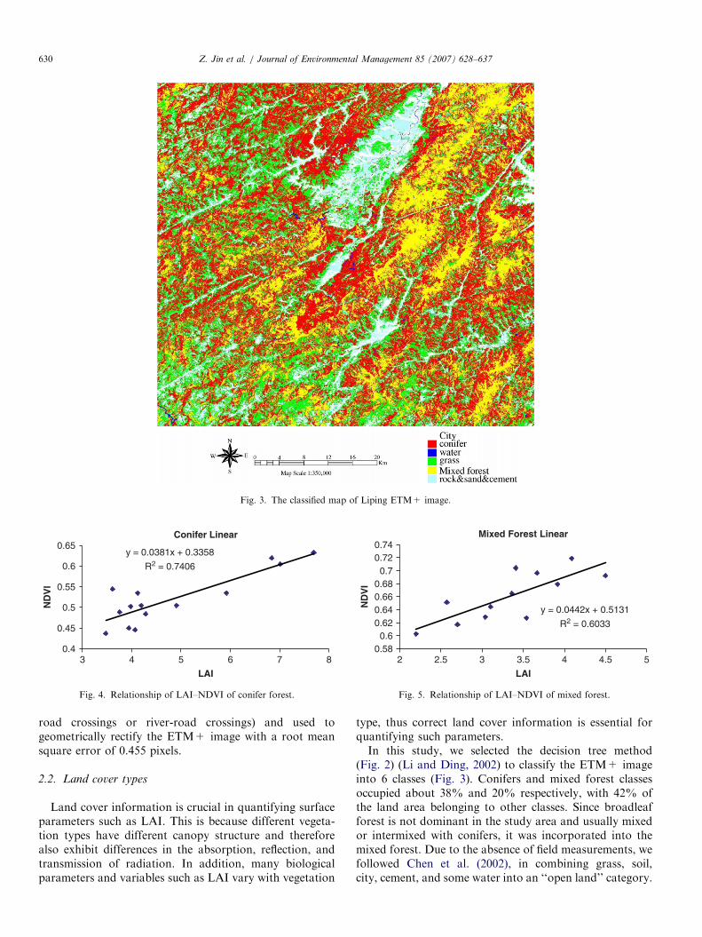
Fig. 3. The classified map of Liping ETM+ image.

Conifer Linear

y = 0.0381x + 0.3358

R2 = 0.7406

0.4

0.45

0.5

0.55

0.6

0.65

3 5 7

LAI

ND

VI

4 6 8

Fig. 4. Relationship of LAI–NDVI of conifer forest.

Mixed Forest Linear

y = 0.0442x + 0.5131

R2 = 0.6033

0.580.6

0.620.640.660.680.7

0.720.74

2 2.5 3 3.5 4 4.5 5

LAI

ND

VI

Fig. 5. Relationship of LAI–NDVI of mixed forest.

Z. Jin et al. / Journal of Environmental Management 85 (2007) 628–637630

road crossings or river-road crossings) and used togeometrically rectify the ETM+ image with a root meansquare error of 0.455 pixels.

2.2. Land cover types

Land cover information is crucial in quantifying surfaceparameters such as LAI. This is because different vegeta-tion types have different canopy structure and thereforealso exhibit differences in the absorption, reflection, andtransmission of radiation. In addition, many biologicalparameters and variables such as LAI vary with vegetation

type, thus correct land cover information is essential forquantifying such parameters.In this study, we selected the decision tree method

(Fig. 2) (Li and Ding, 2002) to classify the ETM+ imageinto 6 classes (Fig. 3). Conifers and mixed forest classesoccupied about 38% and 20% respectively, with 42% ofthe land area belonging to other classes. Since broadleafforest is not dominant in the study area and usually mixedor intermixed with conifers, it was incorporated into themixed forest. Due to the absence of field measurements, wefollowed Chen et al. (2002), in combining grass, soil,city, cement, and some water into an ‘‘open land’’ category.

ARTICLE IN PRESS

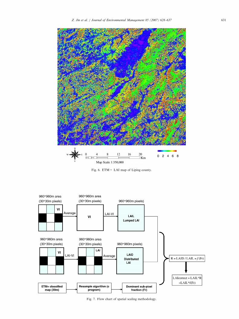
Fig. 6. ETM+ LAI map of Liping county.

Fig. 7. Flow chart of spatial scaling methodology.

Z. Jin et al. / Journal of Environmental Management 85 (2007) 628–637 631

ARTICLE IN PRESSZ. Jin et al. / Journal of Environmental Management 85 (2007) 628–637632

The open land also consists of different forms of naturallandscape within the area of interest. It is defined as a landcover type consisting of recently burned areas, regeneratedareas, and barren soil/rock and wetland areas. Although theLAI of water and city should be 0 or nearly zero, respectively,their areas were very small and the error caused byincorporating them into open land with non-zero LAI couldtherefore be ignored. In this study, the LAI-VI algorithmused for open land was adopted from Chen et al. (2002).

2.3. LAI mapping

LAI mapping was based on the LAI-VI relationship forthe three vegetation types developed from ground LAImeasurements. In August 2002, we used LAI (Pu andGong, 2000) to measure about 30 plots of the coniferousand mixed forest, each plot approximately 150m � 150mor 5� 5 pixels in the ETM+ image. In each plot, we mademeasurements at four locations and calculated the averageLAI for the plot.

3 5 7 83

4

5

6

7

8

9

10

Pixel labled as Conifer

y=0.83539+2.71326

R2=0.4971

Lum

ped

LAI(

960m

)

Distributed LAI(960m)(a)

0 3

0.0

0.5

1.0

1.5

2.0

2.5 y=0.24314∗x+0.66258

R2=0.6471

Pixel labled as Openland

Lum

ped

LAI(

960m

)

Distributed LAI(960m)(c)

4 6

1 2 4 5

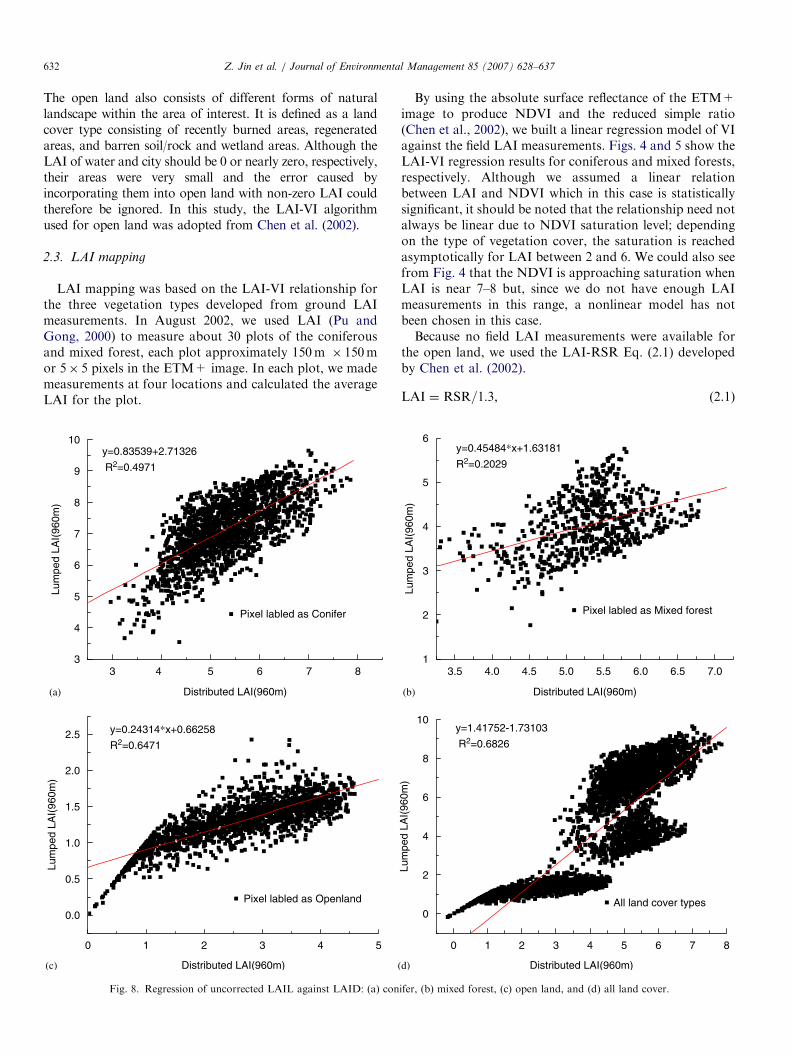
Fig. 8. Regression of uncorrected LAIL against LAID: (a) con

By using the absolute surface reflectance of the ETM+image to produce NDVI and the reduced simple ratio(Chen et al., 2002), we built a linear regression model of VIagainst the field LAI measurements. Figs. 4 and 5 show theLAI-VI regression results for coniferous and mixed forests,respectively. Although we assumed a linear relationbetween LAI and NDVI which in this case is statisticallysignificant, it should be noted that the relationship need notalways be linear due to NDVI saturation level; dependingon the type of vegetation cover, the saturation is reachedasymptotically for LAI between 2 and 6. We could also seefrom Fig. 4 that the NDVI is approaching saturation whenLAI is near 7–8 but, since we do not have enough LAImeasurements in this range, a nonlinear model has notbeen chosen in this case.Because no field LAI measurements were available for

the open land, we used the LAI-RSR Eq. (2.1) developedby Chen et al. (2002).

LAI ¼ RSR=1:3, (2.1)

3.5 4.0 4.5 5.0 5.5 6.0 6.5 7.01

2

3

4

5

6y=0.45484∗x+1.63181

R2=0.2029

Pixel labled as Mixed forest

Lum

ped

LAI(

960m

)

Distributed LAI(960m)(b)

0 3 6 7 8

0

2

4

6

8

10y=1.41752-1.73103

R2=0.6826

All land cover types

Lum

ped

LAI(

960m

)

Distributed LAI(960m)

1 2 4 5

(d)

ifer, (b) mixed forest, (c) open land, and (d) all land cover.

ARTICLE IN PRESSZ. Jin et al. / Journal of Environmental Management 85 (2007) 628–637 633

where RSR is the reduced simple ratio defined based onred, NIR, and shortwave infrared reflectances.

Combining the three LAI-VI algorithms and the ETM+classification, we produced the LAI map (Fig. 6) for LipingCounty using ENVI 3.5 remote sensing image processingsoftware.

3. Spatial scaling model development

3.1. Products for spatial scaling

Methods for LAI spatial scaling were investigated usingLAI images with 960m pixels derived in two ways: (1) fromdistributed calculations (LAID), where LAID was calcu-lated first at 30m resolution and the averaged to 960mresolution pixels; and (2) from lumped calculations (LAIL),in which LAI was calculated using input 30m ETM+vegetation index maps after resampling these to a resolu-tion of 960m. Fig. 7 shows the flowchart of spatial scalingsteps.

0.3 0.4 0.5 0.6 0.7 0.8 0.9 1.00.3

0.4

0.5

0.6

0.7

0.8

0.9

1.0

1.1

y=0.65799∗x+0.35735

R2=0.8142

Pixel labled as Conifer

R=

LAID

/LA

IL

FrConifer(a) (b

0.3 0.4 0.5 0.6

1.0

1.5

2.0

2.5

3.0

3.5

Pixel labled as

R=

LAID

/LA

IL

FrO(c)

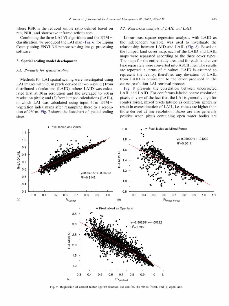
Fig. 9. Regression of correct factor against fraction:

3.2. Regression analysis of LAIL and LAID

Linear least-square regression analysis, with LAID asthe independent variable, was used to investigate therelationship between LAID and LAIL (Fig. 8). Based onthe lumped land cover map, each of the LAID and LAILmaps were separated according to the three cover types.The maps for the entire study area and for each land covertype separately were converted into ASCII files. The resultsare reported in terms of r2 values. LAID is assumed torepresent the reality; therefore, any deviation of LAILfrom LAID is equivalent to the error produced in thecoarse resolution LAI retrieval process.Fig. 8 presents the correlation between uncorrected

LAIL and LAID. For coniferous-labeled coarse resolutionpixels, in view of the fact that the LAI is generally high forconifer forest, mixed pixels labeled as coniferous generallyresult in overestimation of LAIL, i.e. values are higher thanthose derived at fine resolution. Biases are also generallypositive when pixels containing open water bodies are

0.3 0.4 0.5 0.6 0.7 0.8 0.9 1.0 1.10.8

1.0

1.2

1.4

1.6

1.8

2.0

y=-0.95902∗x+1.94239

R2=0.6017

Pixel labled as Mixed Forest

R=

LAID

/LA

IL

FrMixed Forest)

0.7 0.8 0.9 1.0 1.1

y=-2.90288∗x+4.00222

R2=0.7963

Openland

penland

(a) conifer, (b) mixed forest, and (c) open land.

ARTICLE IN PRESSZ. Jin et al. / Journal of Environmental Management 85 (2007) 628–637634

labeled as vegetation. In contrast, mixed pixels labeled asopen land commonly have underestimated LAI values(Fig. 8c). In Fig. 8b, for the mixed forest-labeled coarseresolution pixels, overestimation of LAIL occurs when theycontain significant fractions of conifers, while under-estimation often occurs when they contain open land. Itis thus evident that ignoring sub-pixel land cover-typeinformation induces either positive or negative bias in LAIestimation. These biases depend on the dominant cover-type assigned to a lumped pixel (which is typically mixed).So the key part of the spatial scaling model developmentis to use sub-pixel land cover information to correctthe LAIL.

3.3. Spatial scaling model

A C program was used to produce an ASCII file forcover-type area fractions within each 960m pixel based onthe known sub-pixel information from the 30m resolutiondata. This step is most vital since the scaling algorithms

3 4 5 7 102

3

4

5

6

7

8

Distributed LAI(960m)

y=0.65504∗x+0.65656

R2=0.5725

Pixel labled as Conifer

Cor

rect

ed L

AI(

960m

)

(a)

0.0 0.5 1.0 1.5 2.0 2.5

0

1

2

3

4

5

6

y=3.25288∗x-1.57245

R2=0.8395

Pixel labled as Openland

Cor

rect

ed L

AI(

960m

)

Distributed LAI(960m)(c) (d

6 8 9

(b

Fig. 10. Regression of corrected LAIL against LAID: (a) coni

could not be derived without the knowledge of cover-typearea fractions (conifers, mixed forest, open land).Since the goal of spatial scaling is to compute the LAI

values from coarse resolution sensor data in such a mannerthat they equal the arithmetic average of the LAI valuesderived from fine resolution sensor data (Tian et al., 2002),the corrections of LAIL are based on the regressioncoefficients retrieved by correlating the correction factor R

and each dominant cover-type fraction within the uniquelylabeled coarse pixel. The relationships are as follows:

R ¼ LAID=LAIL; (3.1)

Rtype ¼ anFrtype þ b, (3.2)

where Frtyoe is the fraction of the dominant cover type; a, b

are the linear regression coefficients for a particulardominant cover type.Fig. 9 shows the relationships between the correction

factor R and the dominant fraction within each lumpedpixel. It is apparent that: (1) strong positive or negative

3.0 3.5 4.0 4.5 5.0 5.5 6.0 6.5 7.0

2.5

3.0

3.5

4.0

4.5

5.0

5.5

6.0

6.5

y=0.46447∗x+2.82003

R2=0.5250

Pixel labled as Mixed Forest

Cor

rect

ed L

AI(

960m

)

Distributed LAI(960m)

0 3 5 6 7

0

1

2

3

4

5

6

7

8

y=0.98107∗x+0.09943

R2=0.9582

All landcover types

Cor

rect

ed L

AI(

960m

)

Distributed LAI(960m))

)

1 2 4 8

fer, (b) mixed forest, (c) open land, and (d) all land cover.

ARTICLE IN PRESS

8

7

6

5

4

3

2

1

00 1 2 3 4 5 6 7 8

Distributed LAI (1KM)

MO

DL

S L

AI (

1KM

)

y=0.89017∗x+0.03565

R2=0.54067

Fig. 11. Regression of uncorrected MODIS LAI against LAID.

Co

rrec

ted

MO

DIS

LA

I (1K

m)

6y=0.8720∗x+0.1224

R2=0.78635

4

3

2

1

00 1 2 3 4 5 6

Distributed LAI (1km)

Fig. 12. Regression of corrected MODIS LAI and LAID.

Z. Jin et al. / Journal of Environmental Management 85 (2007) 628–637 635

linear correlations exist between R and Fr for the threecover types, so it is reasonable to develop the spatial scalingalgorithm using cover-type area fractions; and (2) when Frequals to 1, R equals to 1 as well. This proves that whenusing a linear LAI-VI algorithm, pure coarse resolutionpixels will not cause differences between LAID and LAIL.The more pure a coarse resolution pixel is, the less error theLAIL will have.

According to the three equations in Fig. 9, we developedthe spatial scaling algorithm (Eq. (3.3)):

LAIcorrect ¼ LAILnR ¼ LAILnðanFrtype þ bÞ. (3.3)

For conifers, mixed forest, and open land separately, thealgorithms are, respectively, (3.4), (3.5), and (3.6):

LAIcorrect ¼ LAILnð0:65799nFrconifer þ 0:35735Þ, (3.4)

LAIcorrect ¼ LAILnð�0:95902nFrmixedforest þ 1:94239Þ,

(3.5)

LAIcorrect ¼ LAILnð�2:90288nFropenland þ 4:00222Þ. (3.6)

After using the three equations to correct the LAIL, weemployed linear regression analysis to investigate thecorrelation between corrected LAIL and LAID (Fig. 10).It could readily be seen that after the corrections, thecorrelation between LAIL and LAID was much improvedas the correlation increased from R2 ¼ 0:68 to R2 ¼ 0:96for the entire image. For conifer-labeled coarse resolutionpixels, the correlation increases from R2 ¼ 0:50 toR2 ¼ 0:57, for mixed forest-labeled coarse resolution pixelsfrom R2 ¼ 0:20 to R2 ¼ 0:53, and for open land-labeledcoarse resolution pixels from R2 ¼ 0:65 to R2 ¼ 0:84.These results demonstrate that the spatial scaling algo-rithms developed using sub-pixel information could greatlyreduce the error in coarse resolution LAI mapping. Thus, ifland cover-type information is available at high resolution,the above algorithms could be used to correct the coarseresolution (MODIS) LAI product.

To test our algorithm, we applied it to a subset of aMODIS LAI product produced by the University ofToronto, similar to that discussed by Liu et al. (1997).The corresponding ETM+ image of the study area consistsof 2048�2048 pixels. Figs. 11 and 12 show the correlationsbetween MODIS LAI and LAID before and aftercorrection, and Fig. 13 includes both original MODISLAI map and the corrected map. From Figs. 11 and 12 it isevident that the linear correlation between correctedMODIS LAI and LAID was stronger than betweenuncorrected MODIS LAI and LAID. After the correction,the coefficient of determination R2 increased from 0.54 to0.79. The spatial scaling algorithm using sub-pixel infor-mation therefore significantly reduced the error in theMODIS LAI product. It also demonstrated that sub-pixelclassification information for coarse resolution data is ofgreat importance in the spatial scaling process.

4. Discussion

If only coarse resolution images are available for an area,a meaningful spatial scaling is severely limited. To meet thescaling requirement, the traditional practice in landclassification based on ‘‘hard labeling’’ may be replacedwith ‘‘soft labeling’’ approaches, i.e., giving the percentageof major cover types within each pixel. This soft classifica-tion approach has been successfully demonstrated byDeFries et al. (1997). However, it is generally difficult toapply the soft classification approach in case of multiplecover types through spectral unmixing, because the uniquedimensions of optical remote sensing are generally smallerthan the dimensions of surface variability (Verstrate et al.,1996). Therefore, greater attention should be paid toregional and global land cover mapping at high resolution.

ARTICLE IN PRESS

Fig. 13. Image of uncorrected MODIS LAI and corrected MODIS LAI (1 km).

Z. Jin et al. / Journal of Environmental Management 85 (2007) 628–637636

This is in agreement with the suggestion by Chen (1999)that at least a high-resolution water area mask is requiredfor spatial scaling of surface parameters.

Examples shown in this article are limited to twodifferent scales and one biophysical parameter. However,the concept of scaling using contextural parameters couldbe applied in other surface parameters (such as FPAR,temperature, etc). In this study, only three types ofvegetation are considered, and the coefficients determinedin our scaling algorithm would be applicable to similarcover types in other regions. However, if we attempt toexpand this method to other regions with different covertypes, new sets of coefficients can be developed byfollowing the examples given in this study.

5. Conclusions

Surface parameters derived at different spatial resolu-tions can be considerably different even though they arederived using the same algorithms, especially when coarseresolution pixels consist of various land cover types. In thisstudy, we developed a spatial scaling algorithm for LAIbetween two scales (30 and 960m) using a Landsat ETM+image of Liping County. The following main conclusionsare drawn:

(1)

Errors in coarse resolution LAI mapping occurredmainly because coarse resolution pixels are generallymixed and they are labeled as the dominant cover typein the LAI retrieval. LAI–NDVI relationships used inthe LAI algorithm are inherently different amongvarious structurally distinct cover types. This suggeststhat regional and global LAI maps produced withoutconsidering the sub-pixel vegetation-type variationwould be in considerable error.

(2)

An effective way of correcting errors in coarseresolution LAI images is to employ sub-pixel landcover information. It is demonstrated that when thisinformation for three major cover types in LipingCounty was derived from a Landsat ETM+ image at30m resolution and used to correct MODIS LAI at

1 km resolution, the error in the MODIS LAI wasgreatly reduced. This reduction in error was shown as alarge increase in the correlation between the MODISLAI and a high resolution LAI map derived using theETM+ image and ground data; the R2 value increasedfrom 0.54 to 0.79 after performing the correction usingsub-pixel land cover fraction information. Our resultsdemonstrate the need for high resolution land covermaps at regional and global scales for the purpose ofaccurate mapping of biophysical parameters which areland cover-dependent.

References

Atkinson, P.M., Dunn, R., Harrison, A.R., 1996. Measurement error in

reflectance data and its implications for regularizing the variogram.

International Journal of Remote Sensing 17, 3735–3750.

Chen, J.M., 1999. Spatial scaling of a remote sensed surface parameter by

contexture. Remote Sensing Environment 69, 30–42.

Chen, J.M., Pavlic, G., Brown, L., Cihlar, J., Leblanc, S.G., White, H.P.,

Hall, R.J., Peddle, D.R., King, D.J., Trofymow, J.A., Swift, E., Van

der Sanden, J., Pellikka, P.K.E., 2002. Derivation and validation of

Canada-wide coarse-resolution leaf area index maps using high-

resolution satellite imagery and ground measurements. Remote

Sensing of Environment 80, 165–184.

DeFries, R., Hansen, M., Steininger, M., Dubayah, R., Sohlberg, R.,

Townshend, J., 1997. Sub-pixel forest cover in central Africa from

multisensor, multitemporal data. Remote Sensing of Environment 60,

228–246.

Friedl, M.A., Davis, F.W., Michaelsen, D.J., Moritz, M.A., 1995. Scaling

and uncertainty in the relationship between the NDVI and land surface

biophysical variables: an analysis using a scene simulation model and

data from FIFE. Remote Sensing of Environment 54, 233–246.

Hall, F.G., Huemmrich, K.F., Goetz, S.J., Sellers, P.J., Nickeson, J.E.,

1992. Satellite remote sensing of surface energy balance: success,

failures, and unresolved issues in FIFE. Journal of Geophysical

Research 97 (D17), 19061–19089.

Hay, G.J., Niemann, K.O., Goodenough, D.G., 1997. Spatial thresholds,

image-objects and upscaling: a multiscale evaluation. Remote Sensing

of Environment 62, 1–19.

Hui, Feng-ming, Tian, Qing-jiu, 2003. Research and quantitative analysis

of the correlation between vegetation and leaf area index. Remote

Sensing Information 2, 10–13 (in Chinese).

Li, Yan, Ding, Sheng-yan, 2002. The decision tree classification and its

application research in land cover [J]. Remote Sensing Technology and

Application 17 (1), 6–11 (In Chinese).

ARTICLE IN PRESSZ. Jin et al. / Journal of Environmental Management 85 (2007) 628–637 637

Liu, J., Chen, J.M., Cihlar, J., Park, W.M., 1997. A process-based boreal

ecosystem productivity simulator using remote sensing inputs. Remote

Sensing of Environment 62, 158–175.

Pu, Rui-liang, Gong, Peng, 2000. Heperspectral Remote Sensing and it’s

Applications [M]. Higher Education Press, Beijing (in Chinese).

Qi, Y., Wu, J., 1996. Effects of changing spatial resolution on the results of

landscape pattern analysis using spatial autocorrelation indices.

Landscape Ecology 11, 39–49.

Tanre, D., Deroo, C., Duhaut, P., et al., 1986. The Second Simulation of

the Satellite in the Solar Spectrum (6S) User Guide. UST.de Lille,

France: L absoratoired’ Optique Atmospherique.

Tian, Y., Woodcock, C.E., Wang, Y., Privette, J., Shabanov, N.V., Zhou, L.,

Zhang, Y., Buuermann, W., Dong, J., Veikkanen, B., Hame, T., Anderson,

K., Ozdogan, M., Knyazikhin, Y., Myneni, R.B., 2002. Multiscale analysis

and validation of the MODIS LAI product over Maun, Botswana. II.

Sampling Strategy. Remote Senssing Environment 83 (3), 431–441.

Verstrate, M.M., Pinty, B., Myneni, R.B., 1996. Potential and limitations

of information extraction on the terrestrial biosphere from satellite

remote sensing. Remote Sensing of Environment 58, 201–214.

Wu, J., Dennis, E., 2000. Multiscale analysis of landscape heterogeneity:

scale variance and pattern Metrics Jianguo. Geographic Information

Science 6 (1), 6–19.