spatial statistics with image analysis - lunds universitet · spatial statistics with image...
TRANSCRIPT

Spatial Statistics Spatial Examples More
Spatial Statistics with Image Analysis
Johan Lindstrom1
1Mathematical StatisticsCentre for Mathematical Sciences
Lund University
LundOctober 1, 2015
Johan Lindstrom - [email protected] Spatial Statistics 1/31
Spatial Statistics Spatial Examples More
Outline
Spatial Statistics with Image AnalysisBayesian statisticsHierarchical modellingEstimation Procedures
Spatial StatisticsStochastic FieldsGaussian Markov Random FieldsImage Reconstruction
ExamplesEnvironmental DataCorrupted PixelsNDVI
Learn more
Johan Lindstrom - [email protected] Spatial Statistics 2/31
Spatial Statistics Spatial Examples More Bayesian statistics Hierarchical Estimation
A Statistical Approach
◮ All measurements contain random measurementerrors/variation.
◮ Most natural phenomena have natural randomvariation.
◮ Often the uncertainty of an estimate is, at least, asimportant as the estimate itself.
◮ We need to describe and model random variation anduncertainties!
Johan Lindstrom - [email protected] Spatial Statistics 3/31

Spatial Statistics Spatial Examples More Bayesian statistics Hierarchical Estimation
Bayesian modelling
We assume that there is some unknown truth, that wewould like to find out about. This “reality” can bemeasured, usually with measurement variation, and oftenonly partially.
Bayesian modelling
A Bayesian model consists of◮ A prior, “a priori”, model for reality, x, given by the
probability density π(x).◮ A conditional model for data, y, given reality, with
density p(y|x).
The prior can be expanded into several layers creating aBayesian hierarchical model.
Johan Lindstrom - [email protected] Spatial Statistics 4/31
Spatial Statistics Spatial Examples More Bayesian statistics Hierarchical Estimation
Bayes’ Formula
How should the prior and data model be combined to makestatements about the reality x, given observations of y?
Bayes’ Formula
p(x|y) = p(y|x)π(x)p(y)
=p(y|x)π(x)∫
x′∈Ω p(y|x′)π(x′) dx′
p(x|y) is called the posterior, or “a posteriori”, distribution.
Often, only the proportionality relation
p(x|y) ∝ p(x,y) = p(y|x)π(x)
is needed, when seen as a function of x.
Johan Lindstrom - [email protected] Spatial Statistics 5/31
Spatial Statistics Spatial Examples More Bayesian statistics Hierarchical Estimation
Hierarchical Models
◮ We often have some prior knowledge of the reality.◮ Given knowledge of the true reality, what can we say
about images and other data?◮ Construct a model for observations given that we know
the truth.◮ Given data, what can we say about the unknown
reality?This is the inverse problem.
Johan Lindstrom - [email protected] Spatial Statistics 6/31

Spatial Statistics Spatial Examples More Bayesian statistics Hierarchical Estimation
Bayesian hierarchical modelling (BHM)
A hierarchical model is constructed by systematicallyconsidering components/features of the data, and how/whythese features arise.
Bayesian hierarchical modelling
A Bayesian hierarchical model typically consists of (at least)
Data model, p(y|x): Describing how observations ariseassuming known latent variables x.
Latent model, p(x|θ): Describing how the latent variables(reality) behaves, assuming known parameters.
Parameters, π(θ): Describing our, sometimes vauge, priorknowledge of the parameters.
Johan Lindstrom - [email protected] Spatial Statistics 7/31
Spatial Statistics Spatial Examples More Bayesian statistics Hierarchical Estimation
Estimation Procedures
Maximum A Posteriori (MAP): Maximise the posteriordistribution p(x|y) with respect to x.
◮ Standard optimisation methods◮ Specialised procedures, using the model
structure
Simulation: Simulate samples from the posteriordistribution p(x|y). Estimate statisticalproperties from these samples. The samples canbe seen as representative “possible realities”,given the available data.
◮ Markov chain Monte Carlo (MCMC)◮ Gibbs sampling
Johan Lindstrom - [email protected] Spatial Statistics 8/31
Spatial Statistics Spatial Examples More Fields GMRF Reconstruction
Image Reconstruction
Spatial Interpolation
Given observations at some locations (pixels),y(ui), i = 1 . . .nwe want to make statements about the value atunobserved location(s), x(u0).
The typical model consists of a latent Gaussian field
x ∈ N (μ,Σ) ,
observed at locations ui, i = 1, . . . ,n, with additive Gaussiannoise (nugget or small scale variability)
yi = x(ui)+ εi εi ∈ N(
0,σ2ε
).
Johan Lindstrom - [email protected] Spatial Statistics 9/31
Spatial Statistics Spatial Examples More Fields GMRF Reconstruction
Stochastic Fields
To perform the reconstruction (interpolation) we need amodel for the spatial dependence between locations (pixels).
1. Assume a latent Gaussian field
x ∈ N (μ,Σ) .
2. Assume a regresion model for μ = Bβ.
3. Assume a parametric (stationary) model for thedependence (covariance)
Σi,j = C(x(ui), x(uj)) = r(ui,uj;θ) = r(∥∥ui − uj
∥∥ ;θ).
r(ui,uj;θ) is called the covariance function.
Johan Lindstrom - [email protected] Spatial Statistics 10/31
Spatial Statistics Spatial Examples More Fields GMRF Reconstruction
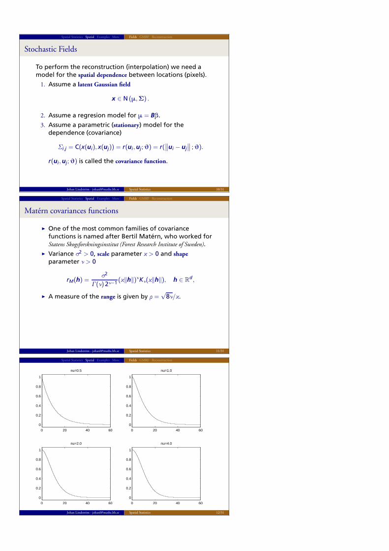
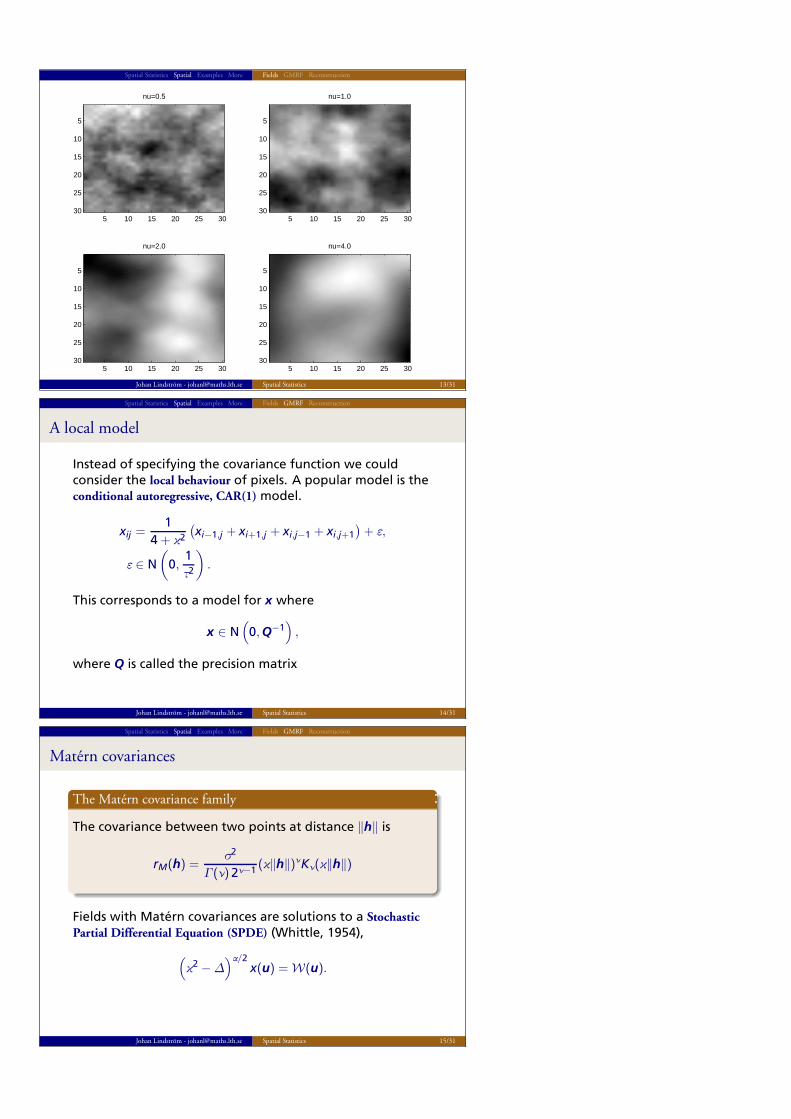
Matern covariances functions
◮ One of the most common families of covariancefunctions is named after Bertil Matern, who worked forStatens Skogsforskningsinstitut (Forest Research Institute of Sweden).
◮ Variance σ2 > 0, scale parameter κ > 0 and shapeparameter ν > 0
rM(h) =σ2
Γ(ν)2ν−1 (κ‖h‖)νKν(κ‖h‖), h ∈ Rd,
◮ A measure of the range is given by ρ =√
8ν/κ.
Johan Lindstrom - [email protected] Spatial Statistics 11/31
Spatial Statistics Spatial Examples More Fields GMRF Reconstruction
0 20 40 60
0
0.2
0.4
0.6
0.8
1
nu=0.5
0 20 40 60
0
0.2
0.4
0.6
0.8
1
nu=1.0
0 20 40 60
0
0.2
0.4
0.6
0.8
1
nu=2.0
0 20 40 60
0
0.2
0.4
0.6
0.8
1
nu=4.0
Johan Lindstrom - [email protected] Spatial Statistics 12/31
Spatial Statistics Spatial Examples More Fields GMRF Reconstruction
nu=0.5
5 10 15 20 25 30
5
10
15
20
25
30
nu=1.0
5 10 15 20 25 30
5
10
15
20
25
30
nu=2.0
5 10 15 20 25 30
5
10
15
20
25
30
nu=4.0
5 10 15 20 25 30
5
10
15
20
25
30
Johan Lindstrom - [email protected] Spatial Statistics 13/31
Spatial Statistics Spatial Examples More Fields GMRF Reconstruction
A local model
Instead of specifying the covariance function we couldconsider the local behaviour of pixels. A popular model is theconditional autoregressive, CAR(1) model.
xij =1
4 + κ2
(xi−1,j + xi+1,j + xi,j−1 + xi,j+1
)+ ε,
ε ∈ N(
0,1τ2
).
This corresponds to a model for x where
x ∈ N(
0,Q−1),
where Q is called the precision matrix
Johan Lindstrom - [email protected] Spatial Statistics 14/31
Spatial Statistics Spatial Examples More Fields GMRF Reconstruction
Matern covariances
The Matern covariance family
The covariance between two points at distance ‖h‖ is
rM(h) =σ2
Γ(ν)2ν−1 (κ‖h‖)νKν(κ‖h‖)
Fields with Matern covariances are solutions to a StochasticPartial Differential Equation (SPDE) (Whittle, 1954),
(κ2 −Δ
)α/2x(u) = W(u).
Johan Lindstrom - [email protected] Spatial Statistics 15/31
Spatial Statistics Spatial Examples More Fields GMRF Reconstruction
Lattice on R2
Order α = 1 (ν = 0):
κ2
1
︸ ︷︷ ︸(C)
+
−1−1 4 −1
−1
︸ ︷︷ ︸≈−Δ (G)
Order α = 2 (ν = 1):
κ4
1
︸ ︷︷ ︸(C)
+2κ2
−1−1 4 −1
−1
︸ ︷︷ ︸≈−Δ (G)
+
12 −8 2
1 −8 20 −8 12 −8 2
1
︸ ︷︷ ︸≈Δ2 (G2=GC−1G)
Johan Lindstrom - [email protected] Spatial Statistics 16/31
Spatial Statistics Spatial Examples More Fields GMRF Reconstruction
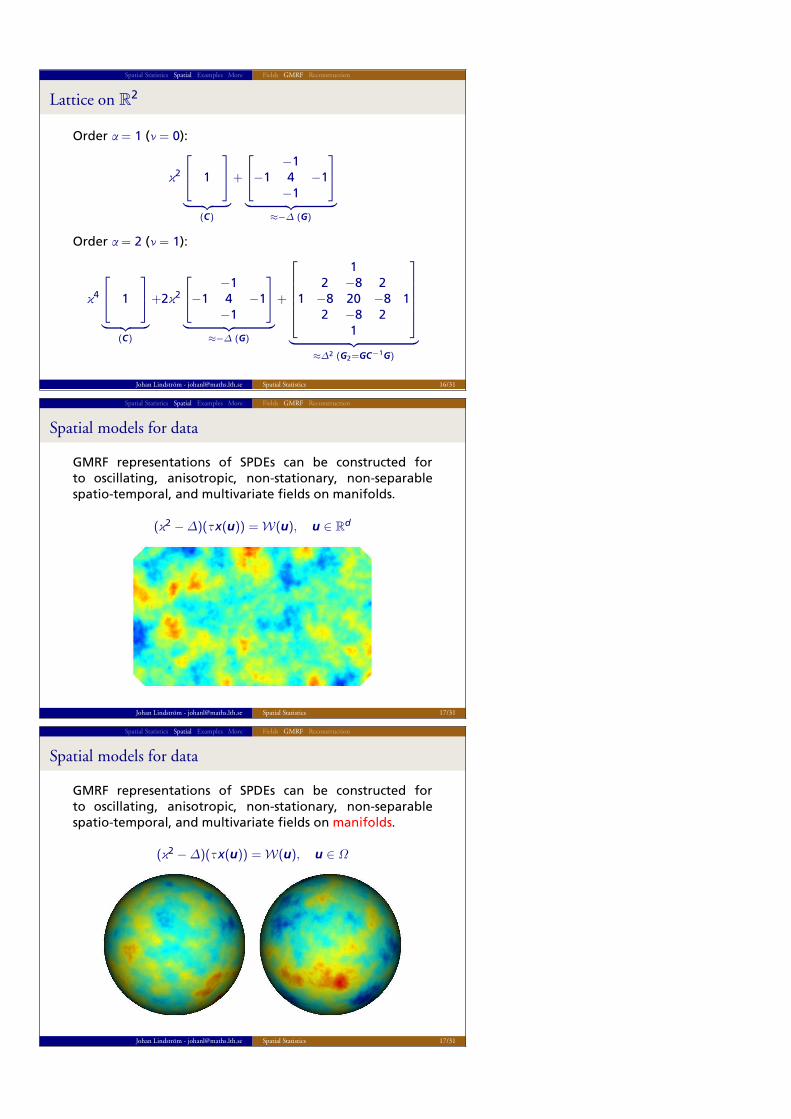
Spatial models for data
GMRF representations of SPDEs can be constructed forto oscillating, anisotropic, non-stationary, non-separablespatio-temporal, and multivariate fields on manifolds.
(κ2 −Δ)(τ x(u)) = W(u), u ∈ Rd
Johan Lindstrom - [email protected] Spatial Statistics 17/31
Spatial Statistics Spatial Examples More Fields GMRF Reconstruction
Spatial models for data
GMRF representations of SPDEs can be constructed forto oscillating, anisotropic, non-stationary, non-separablespatio-temporal, and multivariate fields on manifolds.
(κ2 −Δ)(τ x(u)) = W(u), u ∈ Ω
Johan Lindstrom - [email protected] Spatial Statistics 17/31
Spatial Statistics Spatial Examples More Fields GMRF Reconstruction
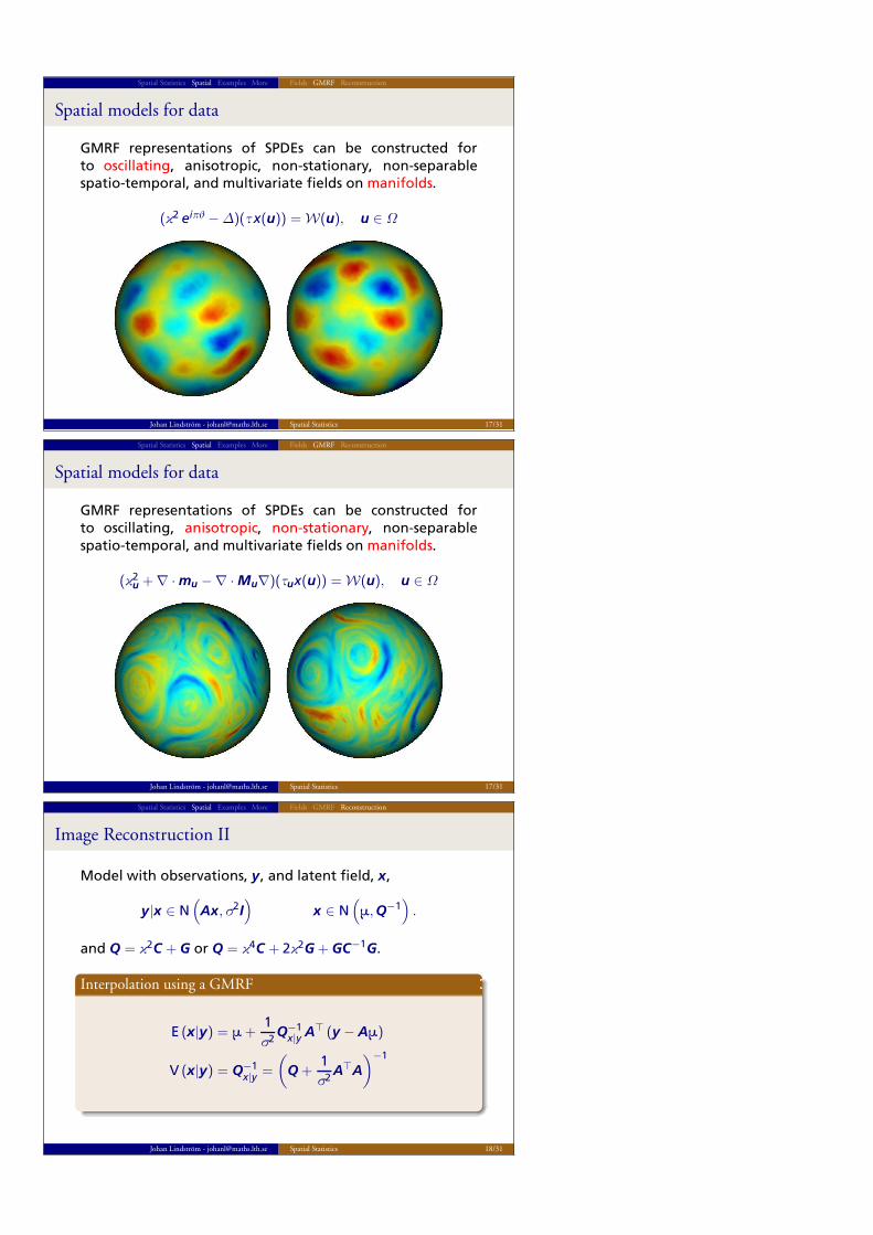
Spatial models for data
GMRF representations of SPDEs can be constructed forto oscillating, anisotropic, non-stationary, non-separablespatio-temporal, and multivariate fields on manifolds.
(κ2 eiπθ −Δ)(τ x(u)) = W(u), u ∈ Ω
Johan Lindstrom - [email protected] Spatial Statistics 17/31
Spatial Statistics Spatial Examples More Fields GMRF Reconstruction
Spatial models for data
GMRF representations of SPDEs can be constructed forto oscillating, anisotropic, non-stationary, non-separablespatio-temporal, and multivariate fields on manifolds.
(κ2u +∇ · mu −∇ · Mu∇)(τux(u)) = W(u), u ∈ Ω
Johan Lindstrom - [email protected] Spatial Statistics 17/31
Spatial Statistics Spatial Examples More Fields GMRF Reconstruction
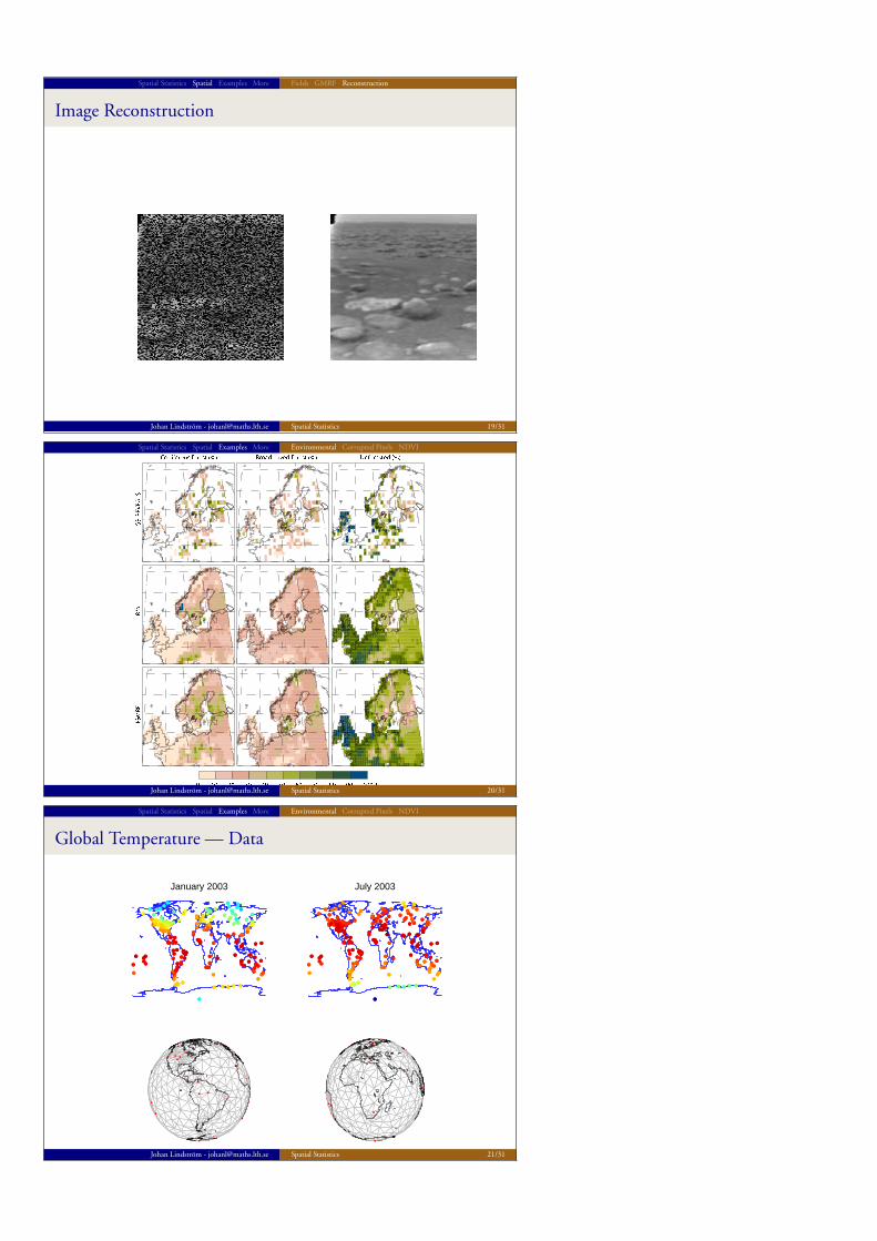
Image Reconstruction II
Model with observations, y, and latent field, x,
y|x ∈ N(
Ax,σ2I)
x ∈ N(μ,Q−1
).
and Q = κ2C + G or Q = κ4C + 2κ2G + GC−1G.
Interpolation using a GMRF
E (x|y) = μ+1σ2 Q−1
x|y A⊤ (y − Aμ)
V (x|y) = Q−1x|y =
(Q +
1σ2 A⊤A
)−1
Johan Lindstrom - [email protected] Spatial Statistics 18/31
Spatial Statistics Spatial Examples More Fields GMRF Reconstruction
Image Reconstruction
Johan Lindstrom - [email protected] Spatial Statistics 19/31
Spatial Statistics Spatial Examples More Environmental Corrupted Pixels NDVI
Johan Lindstrom - [email protected] Spatial Statistics 20/31
Spatial Statistics Spatial Examples More Environmental Corrupted Pixels NDVI
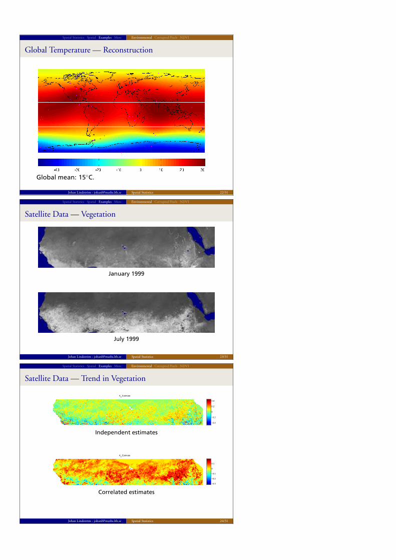
Global Temperature — Data
January 2003 July 2003
Johan Lindstrom - [email protected] Spatial Statistics 21/31
Spatial Statistics Spatial Examples More Environmental Corrupted Pixels NDVI
Global Temperature — Reconstruction
Global mean: 15◦C.
Johan Lindstrom - [email protected] Spatial Statistics 22/31
Spatial Statistics Spatial Examples More Environmental Corrupted Pixels NDVI
Satellite Data — Vegetation
January 1999
July 1999
Johan Lindstrom - [email protected] Spatial Statistics 23/31
Spatial Statistics Spatial Examples More Environmental Corrupted Pixels NDVI
Satellite Data — Trend in Vegetation
K2 Estimate
−0.4
−0.2
0
0.2
0.4
Independent estimates
K2 Estimate
−0.3
−0.2
−0.1
0
0.1
Correlated estimates
Johan Lindstrom - [email protected] Spatial Statistics 24/31
Spatial Statistics Spatial Examples More Environmental Corrupted Pixels NDVI
Image Reconstruction — Corrupted Pixels
◮ Typically we don’t know which pixels that are bad.◮ A better model is then
◮ Assume an underlying image, x.◮ Assume an indicator image for bad pixels, z.◮ Given the indicator we either observe the correct pixel
value from x or noise.
◮ Use Bayes’ formula to compute the distribution for theunknown image (and indicator) given observations andparameters.
Johan Lindstrom - [email protected] Spatial Statistics 25/31
Spatial Statistics Spatial Examples More Environmental Corrupted Pixels NDVI
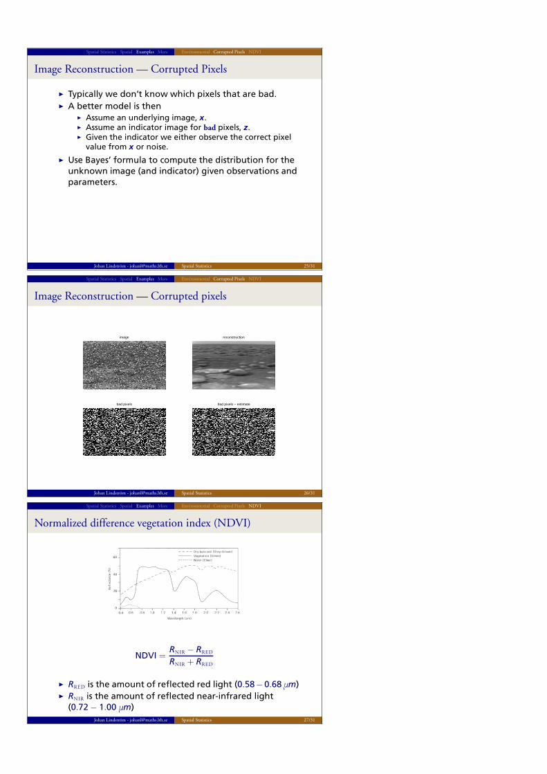
Image Reconstruction — Corrupted pixels
image reconstruction
bad pixels − estimatebad pixels
Johan Lindstrom - [email protected] Spatial Statistics 26/31
Spatial Statistics Spatial Examples More Environmental Corrupted Pixels NDVI
Normalized difference vegetation index (NDVI)
NDVI =RNIR − RRED
RNIR + RRED
◮ RRED is the amount of reflected red light (0.58−0.68 μm)◮ RNIR is the amount of reflected near-infrared light
(0.72 − 1.00 μm)Johan Lindstrom - [email protected] Spatial Statistics 27/31
Spatial Statistics Spatial Examples More Environmental Corrupted Pixels NDVI
Smoothed version of the NDVI Data
Smooth the data to fill in missing values and remove noisedue to cloud cover, etc.
1986 1988 1990
140
160
180
200
Important ecological questions:◮ Plant phenology (start and end of season)◮ Plant productivity (integral)
Johan Lindstrom - [email protected] Spatial Statistics 28/31
Spatial Statistics Spatial Examples More Environmental Corrupted Pixels NDVI
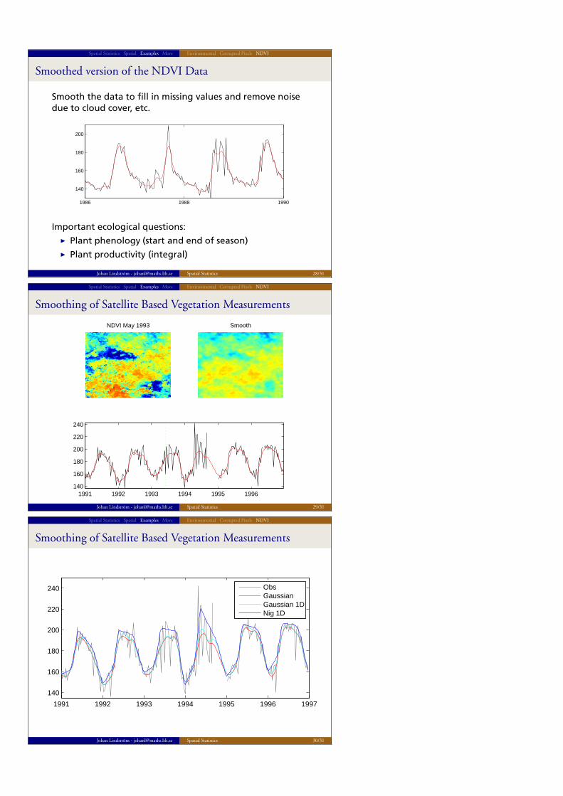
Smoothing of Satellite Based Vegetation Measurements
NDVI May 1993 Smooth
1991 1992 1993 1994 1995 1996140
160
180
200
220
240
Johan Lindstrom - [email protected] Spatial Statistics 29/31
Spatial Statistics Spatial Examples More Environmental Corrupted Pixels NDVI
Smoothing of Satellite Based Vegetation Measurements
1991 1992 1993 1994 1995 1996 1997
140
160
180
200
220
240
ObsGaussianGaussian 1DNig 1D
Johan Lindstrom - [email protected] Spatial Statistics 30/31

Spatial Statistics Spatial Examples More
Learn more!
What?Spatial statistics with image analysis, FMSN20
When?HT2-2015, October–December
Where?Information and Matlab files will be available atwww.maths.lth.se/matstat/kurser/fmsn20masm25/
Who?Lecturer: Johan Lindstrom
MH:319
Johan Lindstrom - [email protected] Spatial Statistics 31/31