Spatially Correlated Stand Structures: 1

A Simulation Approach using Copulas 2

3

John A Kershaw, Jr.1,*

4

Evelyn W. Richards1 5

James B. McCarter2 6

Sven Oborn1 7

8

9

1Faculty of Forestry and Environmental Management, University of New Brunswick, PO Box 10

4400, Fredericton, NB E3B 5A3, Canada 11

2Research Scientist, School of Forest Resources, College of the Environment, University of 12

Washington and Adjunct Associate Professor, Department of Forestry and Environmental 13

Resources, College of Natural Resources, North Carolina State University 14

*corresponding author 15

16

Spatially Correlated Stand Structures: 17

A Simulation Approach using Copulas 18

ABSTRACT 19

In this paper, we propose a simple approach that is capable of generating multispecies 20

stand structures. Based on the method of copulas (Genest and MacKay 1986, Am. Stat. 40:280-21

283), we utilize a normal copula to simulate spatially correlated stand structures. Species 22

composition, diameter, height, and crown ratio distributions of each species, and their correlation 23

with underlying spatial patterns are all controlled by user inputs. Example data sets are used to 24

demonstrate how to estimate required parameters and to compare simulated spatial structures 25

with observed spatial structures. 26

1 ITRODUCTIO 27

Stand structure can be defined as the species composition, size and spatial distribution of 28

trees and other vegetation within a forest stand (Husch et al. 2003). In addition to influencing 29

growth of individual trees (Garcia 2006, Eerikäinen et al. 2007, Fox et al. 2007a, 2007b), stand 30

structure has been shown to influence a number of biotic and abiotic processes within forest 31

stands (Oliver and Larson 1996). Silviculture activities, such as thinning, impact stand structure 32

(Bailey and Tappeiner 1998), and, as a result, influence wildlife populations (Harrington and 33

Tappeiner 2007, Smith et al. 2008, Yamaura et al. 2008), stand dynamics (Saunders and Wagner 34

2008), tree regeneration dynamics (Getzin et al. 2008), and understory vegetation (Kembel and 35

Dale 2006, Gilliam 2007). 36

The past decade has seen a rapid evolution in individual tree growth and yield models. It 37

is generally acknowledged that spatial stand structure is one of the main driving forces behind 38

growth processes, and that stand growth, in return, influences structural composition of 39

woodlands (Pommerening 2006). Several process based models and hybrid models have 40

emerged, and many of these models require spatial data including maps of individual tree 41

locations (e.g., Pretzsch 1992, Pacala et al. 1993, Courbaud 1995). 42

Initialization and testing projections of such models require adequate descriptions of 43

spatial distribution of trees in stands (Pukkala 1988). Collection of such data is generally time 44

consuming and expensive; therefore, very few datasets exists. As a result, several mechanisms 45

for generating spatial data have been proposed (e.g., Stoyan and Penttinen 2000, Valentine et al. 46

2000, Kokkila et al. 2002). Many growth models that require spatial data are highly sensitive to 47

initial stand structure (Valentine et al. 2000, Goreaud et al. 2004, 2006); therefore, it is 48

necessary to have stand structure generators capable of simulating realistic patterns of species 49

composition and spatial and size distribution patterns (Pretzsch 1997). 50

2 EXISTIG APPROACHES 51

Most approaches, such as those of Valentine et al. (2000) and Kokkila et al. (2002), start 52

with a two-dimensional Poisson point process. Tree locations are generated using one of several 53

point process algorithms (e.g., Penridge 1986, Baddeley and Turner 2008). Depending on the 54

algorithm and parameter values, point patterns can vary from regular lattice processes 55

representing a single species, even-aged plantation to a highly clustered pattern as might be 56

found in a mixed species, uneven-aged stand. Some algorithms have the capability of 57

incorporating spatial inhomogeneity (Baddeley and Turner 2008). 58

Once tree locations (points in the point process) are determined, tree size and species 59

attributes are assigned. In some systems, this is done independently of the point pattern (e.g., Ek 60

and Monserud 1974). This approach ignores competitive interactions between individual trees 61

that greatly influence observed stand structure patterns (Valentine et al. 2000, Kokkila et al. 62

2002, Goreaud et al. 2004). Stand structures generated using such processes are often unrealistic 63

(Valentine et al. 2000, Kokkila et al. 2002), and can influence long-term growth projections 64

(Goreaud et al. 2006). 65

To avoid this problem, Valentine et al. (2000) utilized a multistep process to generate 66

initial stand structures used in the AMORPHYS model. In the first step, tree locations are 67

generated. Diameters are then sampled from a target distribution and assigned randomly to the 68

tree locations. The height of each model tree is then calculated from its assigned diameter and 69

distances to its neighbors. Next, crown length of each tree is calculated from its height and 70

distances to its neighbors. Finally, diameter is recalculated based on height and crown length. 71

While this resulting process produces realistic stand structures, the resulting diameter distribution 72

may deviate from the target distribution as a result of the recalculation step and require re-73

simulation (Valentine et al. 2000). 74

An alternative approach is to use a marked point process model (Penttinen et al. 1992, 75

Mateu et al. 1998). In a marked point process model, points are tree locations in a Cartesian 76

coordinate system, and marks are qualitative characteristics such as tree species, or quantitative 77

characteristics such as stem diameter or height (Penttinen et al. 1992). Two correlation functions 78

characterize marked point processes (Penttinen et al. 1992): a pair correlation function which 79

characterizes variability within the system of tree locations; and a mark correlation function 80

which characterizes relationships between different sets of trees (marks) conditional on a 81

distance function. 82

Penttinen et al. (1992) provide excellent examples of the application of marked point 83

processes applied to modeling stand structure. Pommerening et al. (2000) and Mateu et al. 84

(1998) demonstrate the use of marked Gibbs processes to model forest stand structures and 85

discuss how these might be used to simulate forest stand structure. Kokkila et al. (2002) 86

developed a stand structure simulator building upon Penttinen et al.’s (1992), Pommerening et al. 87

(2000), Mateu et al.’s (1998), and others’ work. Kokkila et al. (2002) combine marked Gibbs 88

processes with Markov chain Monte Carlo simulation to produce a flexible stand structure 89

simulator. In addition to the pair and mark correlation functions, they incorporate an additional 90

site potential function which provides additional control on the spatial distribution of trees within 91

simulated stands. 92

While these methods are able to generate structures that statistically resemble example 93

data, no general methods for estimating the parameters required to initialize the simulators are 94

presented (however, see Mateu et al. 1998 and Pommerening et al. 2000). In this paper we 95

present a new approach based on the methods of copulas (Genest and MacKay 1986) and 96

develop a simulation system in R (R Development Core Team 2009). 97

3 MODELLIG APPROACH 98

Standard Normal copulas are utilized to transform random normal variables into 99

correlated variables. Copulas, though widely utilized in several other fields (Accioly and 100

Chiyoshi 2004, Yan 2007), are not very widely known, or at least not widely utilized, in forestry 101

and natural resource management. 102

A copula is a multivariate distribution whose marginals are all uniform over (0, 1). For a 103

p-dimensional random vector U on the unit cube, a copula C is: 104

( ) ( )pupUuUpuuC ≤≤= ,,11Pr,,1 LL . 105

Because any continuous random variable can be transformed to be uniform over (0, 1) by its 106

probability integral transformation, copulas can be used to provide multivariate dependence 107

independent of marginal distributions (Genest and MacKay 1986, Nelsen 2006, Yan 2007). For 108

a complete treatment of the theory and basis of copulas see Nelsen (2006) and for a more 109

descriptive treatment see Genest and MacKay(1986). 110

The basis of our approach assumes there is a correlation between a tree’s characteristics 111

(dbh, total height, and crown ratio) and the area available to the tree (Mitchell 1975, Ford and 112

Diggle 1981, Nance et al. 1988, Valentine et al. 2000). A spatial point process (described below) 113

is used to simulate n tree locations, and we use the polygon areas of a Voronoi tessellation based 114

on point locations generated from a spatial process to define available polygon area (apa). 115

Available polygon areas are standardized : 116

( ) ( ) ( )12−−−= ∑ napaapaapaapaapa , 117

and correlated with vectors of random Normal variables via Wang’s (1998) standard Normal 118

copula algorithm as follows: 119

1) Specify the matrix of partial correlations between available polygon area, diameter and 120

height: 121

=Σ

1,,,

,1,,

,,1,

,,,1

htcrdbhcrapacr

crhtdbhhtapaht

crdbhhtdbhapadbh

crapahtapadbhapa

ρρρ

ρρρ

ρρρ

ρρρ

122

2) Obtain the upper diagonal matrix [A] such that AA′=Σ . We obtain this using 123

Choleski’s decomposition (Andersen et al. 1999) in R. 124

3) Based on the number of points, n, generated with the spatial point process, generate three 125

random standard Normal ( (0,1) ) vectors ( dbh , ht , cr ) of length n. The vectors 126

are column bound with apa to form an augmented matrix, M: 127

[ ]crhtdbhapaM = . 128

4) The columns of M are then correlated using A, the upper diagonal decomposition of Σ : 129

AMZ ⋅= . 130

Because of the structure of A, the first column of M, corresponding to apa , remains 131

unchanged, and dbh , ht , and cr are correlated both with the underlying spatial 132

pattern and the dbh-height-crown ratio relationships. 133

5) The Normal margins are stripped by applying the inverse cumulative Normal probability 134

distribution: 135

( ) ( ) ( )

−−−= htZdbhZapaZU

1Φ1Φ1Φ . 136

U is a standard Normal copula (Wang 1998). 137

6) The correlated size-spatial data are then obtained by applying the appropriate cumulative 138

margin distribution functions, ( )iuiF , to the columns of U. For apa, the cumulative 139

function is the inverse of the standardization formula, or simply the original Voronoi 140

polygon areas. The marginal distribution functions for diameter, height and crown ratio 141

are described below. 142

3.1 Spatial Models 143

We utilize two spatial processes: a Lattice Process and a Thomas Process. The lattice 144

process is used to simulate plantation spacing and is implemented in a custom function in R (R 145

Development Core Team 2009), rlattice. This function utilizes the rlinegrid function (Baddeley 146

and Turner 2008). Angles for the x-oriented lines and y-oriented lines are specified. The x-147

angle and y-angle must be of opposite sign and between 0 and 90 degrees to insure that lines 148

intersect. The desired density (number of trees within the stand) and the xy-ratio must also be 149

specified. The stand area, density and xy-ratio define the spacing of the x and y lines. The xy-150

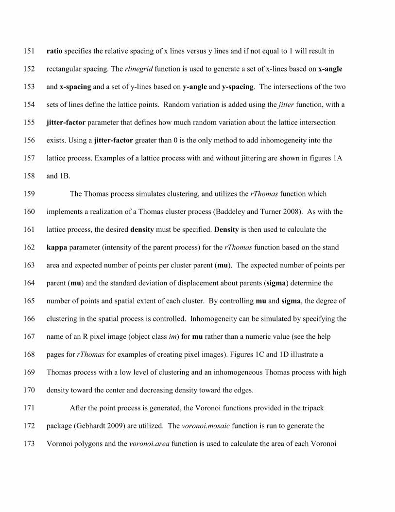
ratio specifies the relative spacing of x lines versus y lines and if not equal to 1 will result in 151

rectangular spacing. The rlinegrid function is used to generate a set of x-lines based on x-angle 152

and x-spacing and a set of y-lines based on y-angle and y-spacing. The intersections of the two 153

sets of lines define the lattice points. Random variation is added using the jitter function, with a 154

jitter-factor parameter that defines how much random variation about the lattice intersection 155

exists. Using a jitter-factor greater than 0 is the only method to add inhomogeneity into the 156

lattice process. Examples of a lattice process with and without jittering are shown in figures 1A 157

and 1B. 158

The Thomas process simulates clustering, and utilizes the rThomas function which 159

implements a realization of a Thomas cluster process (Baddeley and Turner 2008). As with the 160

lattice process, the desired density must be specified. Density is then used to calculate the 161

kappa parameter (intensity of the parent process) for the rThomas function based on the stand 162

area and expected number of points per cluster parent (mu). The expected number of points per 163

parent (mu) and the standard deviation of displacement about parents (sigma) determine the 164

number of points and spatial extent of each cluster. By controlling mu and sigma, the degree of 165

clustering in the spatial process is controlled. Inhomogeneity can be simulated by specifying the 166

name of an R pixel image (object class im) for mu rather than a numeric value (see the help 167

pages for rThomas for examples of creating pixel images). Figures 1C and 1D illustrate a 168

Thomas process with a low level of clustering and an inhomogeneous Thomas process with high 169

density toward the center and decreasing density toward the edges. 170

After the point process is generated, the Voronoi functions provided in the tripack 171

package (Gebhardt 2009) are utilized. The voronoi.mosaic function is run to generate the 172

Voronoi polygons and the voronoi.area function is used to calculate the area of each Voronoi 173

polygon which is is used as our estimate of available polygon area (apa) for each tree. Boundary 174

points are torused by default so that edge points have bounded Voronoi polygons. The Voronoi 175

object returned by the voronoi.mosaic function forms the base of the data frame used to store tree 176

characteristics. 177

3.2 Species – Size Distributions 178

Diameter and height distributions are specified using mixture Weibull distributions (Liu 179

et al. 2002, Zhang and Liu 2006), and crown ratio is specified using a mixture four-parameter 180

Beta distribution. A mixture distribution is defined as a frequency distribution made up of two 181

or more component distributions. The distribution of the ith

individual component is described 182

by a specific probability density function (pdf), ( )xif . Then the general pdf, ( )xf for the mixture 183

distribution is expressed as: 184

( ) ( ) ( ) ( ) ( )xkfkpxfpxfpk

i

xifipxf +++=∑=

= L22111

, 185

where ip = the probability of belonging to component i. In this case, ip is derived from species 186

composition and ( )xif are species-specific distributions. 187

Species composition can be specified in a number of ways including percentiles, 188

quantiles, or actual densities of each species. During the structure simulation process, the 189

specified composition is converted into a frequency distribution ( ip ) and used to randomly 190

assign species to each tree (point). 191

For diameter, the inverse cumulative two-parameter Weibull distribution function is used 192

to obtain values: 193

( )[ ]( )icuibiD /11ln −−= , 194

where iD is diameter of the ith

species corresponding to cumulative probability u; u is a 195

cumulative probability obtained from a standard Normal copula; ib is a species-specific Weibull 196

scale parameter; and ic is a species-specific Weibull shape parameter. Species-specific two-197

parameter Weibull distributions were used for simulating dbh because of the flexibility of the 198

Weibull distribution, wide application in forestry, and readily available methods for estimating 199

the parameters (Bailey and Dell 1973, Hyink and Moser 1983, Little 1983, Robinson 2004). 200

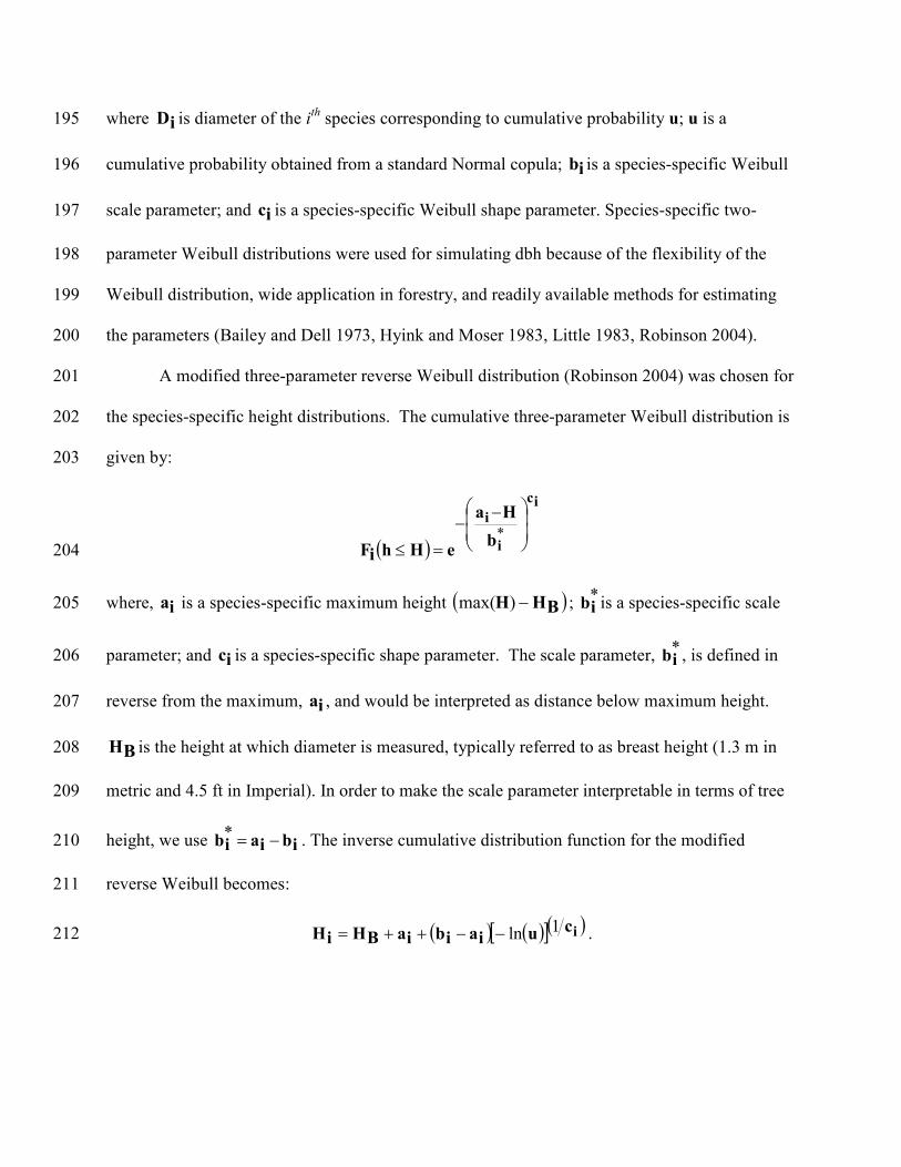
A modified three-parameter reverse Weibull distribution (Robinson 2004) was chosen for 201

the species-specific height distributions. The cumulative three-parameter Weibull distribution is 202

given by: 203

( )

ic

i

i

b

Ha

eHhiF

−−

=≤*

204

where, ia is a species-specific maximum height ( )BHH −)max( ; *ib is a species-specific scale 205

parameter; and ic is a species-specific shape parameter. The scale parameter, *ib , is defined in 206

reverse from the maximum, ia , and would be interpreted as distance below maximum height. 207

BH is the height at which diameter is measured, typically referred to as breast height (1.3 m in 208

metric and 4.5 ft in Imperial). In order to make the scale parameter interpretable in terms of tree 209

height, we use ibiaib −=* . The inverse cumulative distribution function for the modified 210

reverse Weibull becomes: 211

( ) ( )[ ]( )icuiaibiaBHiH 1ln−−++= . 212

Inclusion of BH insures that no tree is shorter than the height at which diameter is measured. 213

Like the two parameter Weibull distribution, parameter estimation for the three-parameter 214

reverse Weibull is relatively straightforward (Robinson 2004). 215

For crown ratio, CR, a 4-parameter Beta distribution (Johnson et al. 1995 pp. 210 - 275) 216

is used. The pdf for the four parameter Beta distribution is given by: 217

( )( ) ( )

1

1

1

)(

−

−−

−−

−−

ΓΓ+Γ

=β

ξλ

ξα

ξλ

ξ

βα

βα CRCRCRf , 218

where α and β are the Beta shape parameters, ξ is the minimum crown ratio, λ is the maximum 219

crown ratio, ( )•Γ is the gamma function, and CR is the observed crown ratio. Simulated crown 220

ratios are obtained using the rbeta function in R using the correlated U(0,1)’s from the Normal 221

copula. The rbeta function is a two parameter Beta distribution and returns a random variable, Z, 222

between 0 and 1. Z is transformed into crown ratio using: 223

( )ξλξ −⋅+= ZCR . 224

The beta parameters are readily estimated using the method of moments or maximum likelihood 225

methods (Johnson et al. 1995 pp. 210 - 275). 226

The mixture distributions are simulated using the following algorithm: 227

1) For the n points generated in the spatial process, species is assigned randomly based on a 228

weighted probability as defined by species composition. 229

2) Once species are assigned, then the species-specific distribution parameters are used to 230

calculate diameter, height, and crown ratio using the correlated U(0,1)’s from the 231

standard Normal copula as cumulative probabilities . 232

The algorithm is implemented in a custom R function q.mixed. 233

4 THE STAD GEERATOR 234

The stand generator is developed in the R statistical package (R Development Core Team 235

2009) and is implemented in a custom R function stand.generate. We utilize three contributed 236

packages: spatstat (Baddeley and Turner 2008); tripack (Gebhardt 2009); and tcltk (Dalgaard 237

2001). The required inputs, structure generation, and visualization are controlled through a 238

series of input windows built using the tcl/tk interface within R version 2.10.1. 239

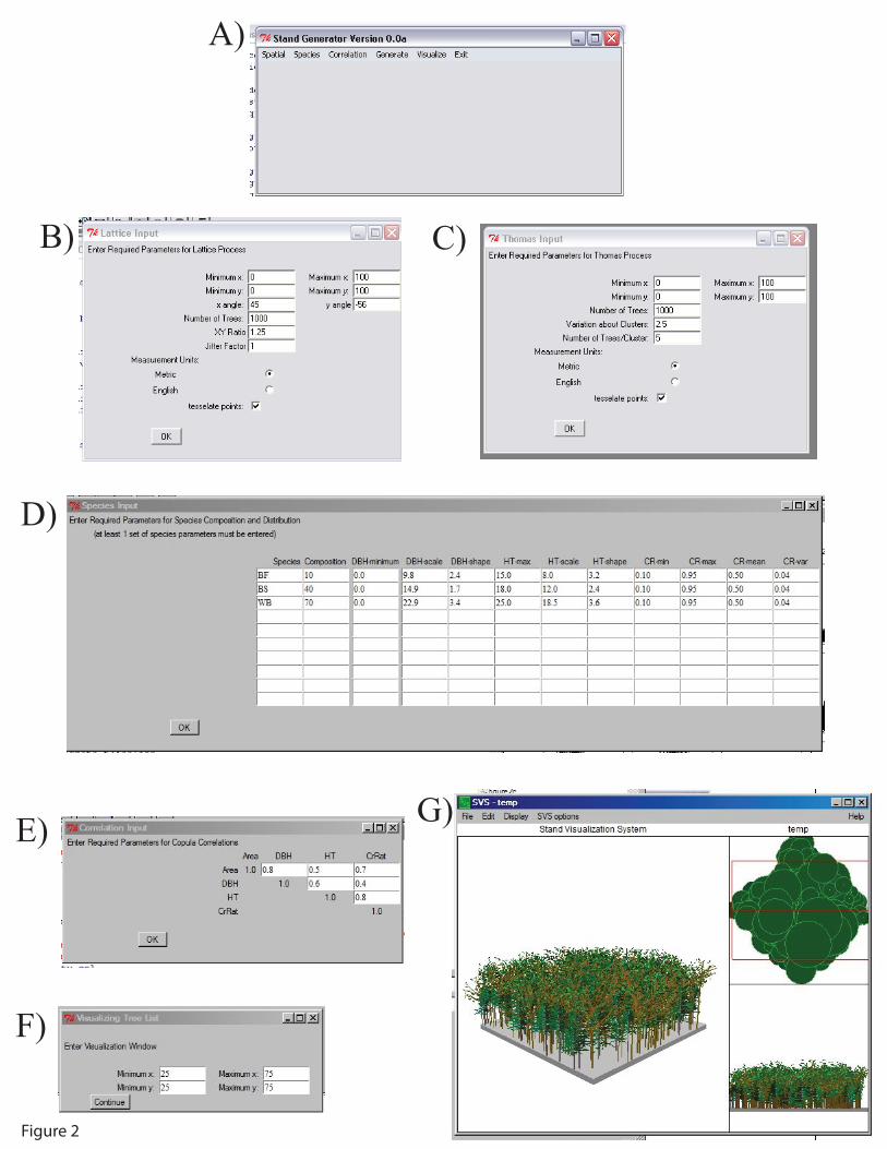
The stand generator starts with a main menu window (Figure 2A). The input is divided 240

into three components: Spatial; Species; and Correlation. The Spatial window (Figs. 2B and 2C) 241

allows users to specify spatial information such as dimensions of the stand, desired density, and 242

underlying spatial models. Currently, only rectangular stand areas are supported. Points are 243

torused around the bounding box so that tree locations near the edge will have complete Voronoi 244

polygons. Torusing can be turned off; however, the functions used to calculate the Voronoi 245

polygon areas delete edge points with unbounded Voronoi polygons. 246

Species composition, diameter, height and crown ratio distribution parameters are 247

specified in the Species window (Fig. 2D). Currently the system allows up to 10 species to be 248

specified. The Correlation window (Fig. 2E) allows the user to specify desired correlations 249

between available tree area, diameter, height, and crown ratio. 250

When the Generate button is pressed, the required inputs are used to generate the spatial 251

processes, the voronoi polygon areas, and the trees’ species-size distributions. The output is 252

stored in a temporary data frame named temp.Trees. Each time Generate is clicked, temp.Trees is 253

over written; therefore, if a user wishes to save results, temp.Trees must be save to a new file 254

before Generate is reclicked. The Visualization window (Fig. 2F) writes an external Stand 255

Visualization System (McGaughey 1997) compatible file and runs SVS (SVS must be installed 256

on the computer) which displays the generated stand structure (Fig. 2G). 257

The R code for the stand generator is available at 258

http://ifmlab.for.unb.ca/People/Kershaw. The stand generator will run on all platforms supported 259

by R; however, the visualization step only runs on Windows-based platforms since it utilizes the 260

stand visualization system which is a Windows-based application. 261

5 EXAMPLES 262

Data from two different studies are used to demonstrate parameter estimation and test 263

simulation results. The first data set is a 4 ha mapped longleaf pine (Pinus palustris Mill.) stand 264

(Platt et al. 1988) consisting of 584 trees. Only diameter at breast height (DBH) and tree 265

locations were measured in this dataset. Total height was predicted using the height – diameter 266

equation found in Shaw and Long (2007). Random error, sampled from a Normal distribution 267

and correlated with available polygon area was added to the predicted heights. Crown ratio was 268

predicted using the crown ratio equation by Acharya (2006)and random error based on the root 269

mean square error was added to the predicted crown ratios from Acharya (2006) so that the 270

resulting predicted crown ratios were correlated with available polygon area. Random errors 271

were added to predicted heights and crown ratios to both add a degree of spatial correlation to 272

the predicted data and reduce correlations within tree parameters. The resulting individual tree 273

summary statistics for this dataset are shown in table 1. 274

The second dataset is a 50 m by 50 m mapped plot located in a mixed species Acadian 275

Forest stand in central New Brunswick. Wooden stakes were surveyed and placed in the ground 276

on a 10 m by 10 m grid. Distance (nearest .01 m) from two adjacent stakes were measured to the 277

face of each tree in each 10m by 10 m block and triangulation, based on side-side-side geometry, 278

was used to determine the xy coordinates of each tree. Tree species was noted, and dbh (nearest 279

0.1 cm) was measured with a diameter tape, and height (nearest 0.1 m) and height to crown base 280

(nearest 0.1 m) were measured with an Optilogic 800LH hypsometer (Opti-Logic Corporation, 281

Tullahoma, TN). There were nine different species in this example: balsam fir (Abies balsamea 282

(L.) Mill.); spruce (mostly black spruce (Picea mariana (Mill.) Britton, Sterns & Poggenb.) with 283

some red spruce (Picea mariana (Mill.) Britton, Sterns & Poggenb.); eastern cedar (Thuja 284

occidentalis L.); eastern hemlock (Tsuga canadensis (L.) Carrière); red maple (Acer rubrum L.); 285

white birch (Betula papyrifera Marsh.); yellow birch (Betula alleghaniensis Britton); white ash 286

(Fraxinus americana L.); and American mountain-ash (Sorbus americana Marsh.).The 287

individual tree summary statistics by species for this dataset are shown in table 1. 288

5.1 Parameter Estimation 289

Thomas spatial processes were used to model spatial locations for both example datasets. 290

Parameters for the Thomas process were estimated using the procedure described by Møller and 291

Waagepetersen (2003 pp. 192 - 197) and Waagepetersen (2008) and implemented in the R 292

function thomas.estK. The current version of the stand structure generator only allows a single 293

spatial process for the entire stand; therefore, only a single process was estimated for the mixed 294

species Acadian Forest dataset. The estimated parameters for the Thomas process are shown in 295

table 2. 296

Maximum likelihood estimates of the Weibull shape and scale parameters for the 297

diameter and height distributions were estimated using a modification of Robinson’s (2004) 298

algorithm. The minimum measured diameter (2.0 cm dbh for the Longleaf Pine dataset and 8.0 299

cm dbh for the Acadian Forest dataset) were used as the truncation points for the two-parameter 300

left-truncated Weibull distribution (Table 3) and the maximum observed height (plus 0.1 m) for 301

each species was used as the location parameter in the three-parameter reverse Weibull 302

distribution (Table 4). The minimum and maximum crown ratios were used as the bounds of the 303

four parameter Beta distribution. The mean and variance of crown ratio was calculated and 304

moment-based parameter recovery used to estimate the two Beta shape parameters (Table 5). 305

The longleaf pine data were distinctly bimodal in the dbh and height distributions; therefore, the 306

data were divided into overstory trees (trees > 24 cm dbh) and understory trees (trees < 24 cm 307

dbh). 308

The correlation matrix used in the standard Normal copula is the matrix of partial 309

correlations between available polygon area and the tree characteristics. Because the marginal 310

distributions are neither Normal nor the same distribution, we used Spearman’s rank correlation 311

coefficient (Zar 1999 pp. 395-398) rather than Pearson’s correction coefficient (Table 6). 312

5.2 Assessment of Simulated Stand Structures 313

Fifty simulated stand structures were generated using the estimated parameters from each 314

example dataset. The simulation results were compared to the observed results using the mark 315

correlation coefficient of Stoyan and Stoyan (1994 pp. 262 - 266) as implemented in the R 316

function markcorr. Observed and simulated mark correlations versus neighborhood radius are 317

shown in figure 3. While the average mark correlations from the simulated stand structures were 318

smoother than observed correlations, individual simulations often produced local peaks at or near 319

the same spatial scales as the observed data. With the exception of the shorter neighborhood 320

radii, the range of correlations from the simulated data included the observed correlations. This 321

was especially obvious in the Longleaf Pine dataset (Fig. 3A). The smaller range of simulated 322

variability observed in the height (Fig. 3C) and crown ratio (Fig. 3E) in the Longleaf Pine dataset 323

was the result of the high correlations with dbh (Table 6) resulting from the prediction of the 324

these variables using dbh. 325

6 DISCUSSIO AD COCLUSIOS 326

The stand structure generator developed in this paper is a simple and efficient method to 327

simulate realistic stand structures. The distributions used to simulate the tree attributes are 328

distributions commonly used in forestry research. The parameters of these distributions are easily 329

estimated from observed data via maximum likelihood methods or moment-based parameter 330

recovery methods. Moment-based parameter recovery methods are especially useful when only 331

stand-level summaries are available (Hyink and Moser 1983). Any distribution could be 332

substituted for those we chose by modifying the input menus and inverse cumulative distribution 333

functions. 334

The use of a Normal copula (Wang 1998) provides an intuitive and fast method for 335

generating the desired spatial dependency. Copulae are applied in many different fields to model 336

complex dependencies (Accioly and Chiyoshi 2004). The critical assumption in the application 337

present in this paper is that available polygon area provides the basic measure of spatial 338

dependency. The available polygon area was proposed by Nance et al. (1988). Here we use 339

Voronoi polygons which are tessellations of the stand area based on perpendicular bisectors of a 340

tree and its immediate neighbors (Bowyer 1981). Nance et al. (1988) proposed weighted 341

polygons, where the division of area was based upon a weighted tree size such that the bisecting 342

line is located further away from the larger tree. This concept is the basis for many distance-343

dependent measures of competition (Tomé and Burkhart 1989, Stage and Ledermann 2008). 344

While we do not produce weighted polygon areas, the copula produces effects similar such that 345

larger trees tend to be located in larger polygons (assuming the correlation coefficient is 346

positive). 347

A limitation to the copula approach is that all species have the same spatial and intra-tree 348

level correlation coefficients. The system proposed by Valentine et al. (2000) has similar 349

limitations; however, systems based on Gibbs processes can have “repulsive potentials” that vary 350

by species producing spatial patterns that vary by species (Kokkila et al. 2002). The advantage of 351

the copula approach over these other approaches is that trees do not have to be spatially shifted 352

based on potentials (Kokkila et al. 2002, Goreaud et al. 2004) or have tree attributes re-simulated 353

to achieve the desired tree and or spatial distributions (Valentine et al. 2000). Eliminating the 354

need for shifting or re-simulating distributions greatly increases the computational efficiency of 355

our system relative to other systems. Further, the use of the correlation structure to determine the 356

tree attributes (ie, dbh, height, and crown ratio) enables simulation of greater levels of variability 357

and more realistic stand structures than predictive systems that often result in lower variation and 358

greater ordering of tree attributes (ie, largest dbh trees tend to be the tallest, etc.). 359

REFERECES 360

Accioly, R. D. M. E. S., and F. Y. Chiyoshi. 2004. Modeling dependence with copulas: a useful 361

tool for field development decision process. Journal of Petroleum Science and 362

Engineering 44:83-91. 363

Acharya, T. P. 2006. Prediction of Distribution for Total Height and Crown Ratio using Normal 364

versus Other Distributions. Unpbl. M.Sc. Thesis. Auburn University. Retrieved April 6, 365

2010, from http://etd.auburn.edu/etd/handle/10415/585. 366

Andersen, E., Z. Bai, C. Bischof, S. Blackford, J. Demmel, J. Dongarra, J. Du Croz, A. 367

Greenbaum, S. Hammarling, A. McKenney, and D. Sorensen. 1999. LAPACK Users' 368

Guide, Third Edition. SIAM, . Retrieved April 5, 2010, from 369

http://www.netlib.org/lapack/lug/index.html. 370

Baddeley, A., and R. Turner. 2008. spatstat: Spatial Point Pattern analysis, model-fitting, 371

simulation, tests. Retrieved April 5, 2010, from http://www.spatstat.org/. 372

Bailey, J. D., and J. C. Tappeiner. 1998. Effects of thinning on structural development in 40- to 373

100-year-old Douglas-fir stands in western Oregon. Forest Ecology and Management 374

108:99-113. 375

Bailey, R. L., and T. R. Dell. 1973. Quantifying Diameter Distributions with the Weibull 376

Function. Forest Science 19:97-104. 377

Bowyer, A. 1981. Computing Dirichlet tessellations. The Computer Journal 24:162-166. 378

Courbaud, B. 1995. Modélisation de la croissance en forêt irrégulière. Perspectives pour les 379

pessières irrégulières de montagne. [Modelling growth in an uneven forest. Anticipating 380

development of irregular Picea abies stands in mountain environments.]. Revue 381

Forestière Française 48:173-182. 382

Dalgaard, P. 2001. The R-Tcl/Tk interface. In: K. Hornik & F. Leisch (eds.), DSC 2001 383

Proceedings of the 2nd International Workshop on Distributed Statistical Computing:1-9. 384

Eerikäinen, K., J. Miina, and S. Valkonen. 2007. Models for the regeneration establishment and 385

the development of established seedlings in uneven-aged, Norway spruce dominated 386

forest stands of southern Finland. Forest Ecology and Management 242:444-461. 387

Ek, A. R., and R. A. Monserud. 1974. FOREST: a computer model for simulating the growth and 388

reproduction of mixed species forest stands. Page 72. Report, School of Natural 389

Resources, College of Agriculture and Life Sciences, University of Wisconsin, Madison, 390

WI. 391

Ford, E. D., and P. J. Diggle. 1981. Competition for Light in a Plant Monoculture Modelled as a 392

Spatial Stochastic Process. Annals of Botany 48:481-500. 393

Fox, J. C., H. Bi, and P. K. Ades. 2007a. Spatial dependence and individual-tree growth models: 394

I. Characterising spatial dependence. Forest Ecology and Management 245:10-19. 395

Fox, J. C., H. Bi, and P. K. Ades. 2007b. Spatial dependence and individual-tree growth models. 396

II. Modelling spatial dependence. Forest Ecology and Management 245:20-30. 397

Garcia, O. 2006. Scale and spatial structure effects on tree size distributions: implications for 398

growth and yield modelling. Canadian Journal of Forest Research 36:2983-2993. 399

Gebhardt, A. 2009. tripack: Triangulation of irregularly spaced data. Retrieved April 5, 2010, 400

from http://cran.r-project.org/index.html. 401

Genest, C., and J. MacKay. 1986. The Joy of Copulas: Bivariate Distributions with Uniform 402

Marginals. The American Statistician 40:280-283. 403

Getzin, S., T. Wiegand, K. Wiegand, and F. He. 2008. Heterogeneity influences spatial patterns 404

and demographics in forest stands. Journal of Ecology 96:807-820. 405

Gilliam, F. S. 2007. The Ecological Significance of the Herbaceous Layer in Temperate Forest 406

Ecosystems. Bioscience 57:845-858. 407

Goreaud, F., I. Alvarez, B. Courbaud, and F. de Coligny. 2006. Long-Term Influence of the 408

Spatial Structure of an Initial State on the Dynamics of a Forest Growth Model: A 409

Simulation Study Using the Capsis Platform. Simulation 82:475-495. 410

Goreaud, F., B. Loussier, M. A. Ngo Bieng, and R. Allain. 2004. Simulating realistic spatial 411

structure for forest stands : a mimetic point process. Interdisciplinary Spatial Statistics 412

Workshop:22 p. 413

Harrington, T. B., and J. C. Tappeiner. 2007. Silvicultural Guidelines for Creating and Managing 414

Wildlife Habitat in Westside Production Forests. Pages 49-59. General Technical Report, 415

USDA, Forest Service, Pacific Northwest Research Station. Retrieved from 416

http://ifmlab.for.unb.ca/People/Kershaw/PDF_Library/H/HarringtonTB2007b.pdf. 417

Husch, B., T. W. Beers, and J. A. J. Kershaw. 2003. Forest Mensuration, 4th edition. Wiley, New 418

York. 419

Hyink, D. M., and J. W. J. Moser. 1983. A Generalized Framework for Projecting Forest Yield 420

and Stand Structure Using Diameter Distributions. Forest Science 29:85-95. 421

Johnson, N. L., S. Kotz, and N. Balakrishnan. 1995. Continuous Univariate Distributions, 2nd 422

edition. Wiley, New York. 423

Kembel, S. W., and M. R. Dale. 2006. Within-stand spatial structure and relation of boreal 424

canopy and understorey vegetation. Journal of Vegetation Science 17:783-790. 425

Kokkila, T., A. Mäkelä, and E. Nikinmaa. 2002. A Method for Generating Stand Structures 426

Using Gibbs Marked Point Process. Silva Fennica 36:265-277. 427

Little, S. N. 1983. Weibull diameter distributions for mixed stands of western conifers. Canadian 428

Journal of Forest Research 13:85-88. 429

Liu, C., L. Zhang, C. J. Davis, D. S. Solomon, and J. H. Gove. 2002. A Finite Mixture Model for 430

Characterizing the Diameter Distributions of Mixed-Species Forest Stands. Forest 431

Science 48:653-661. 432

Mateu, J., J. Uso´, and F. Montes. 1998. The spatial pattern of a forest ecosystem. Ecological 433

Modelling 108:163-174. 434

McGaughey, R. J. 1997. Visualizing forest stand dynamics using the stand visualization system. 435

1997 ACSM/ASPRS Annual Convention and Exposition 4:248-257. 436

Mitchell, K. J. 1975. Dynamics and Simulated Yield of Douglas-fir. Forest Science Monographs 437

17:39. 438

Møller, J., and R. P. Waagepetersen. 2003. Statistical Inference and Simulation for Spatial Point 439

Processes. Chapman Hall/CRC Press, New York. 440

Nance, W. L., J. E. Grissom, and W. R. Smith. 1988. A new competition index based on 441

weighted and constrained area potentially available. Pages 134-142. General Technical 442

Report, USDA, Forest Service, Ek, A. R., Shifley, S. R., and Burk, T. E. (eds.) Forest 443

growth modeling and prediction. Vol. 1. Proceedings of the August 23-27 IUFRO 444

Conference, Minneapolis, Minnesota. North Central Forest Experiment Station. 445

Nelsen, R. B. 2006. An Introduction to Copulas, 2nd edition. Springer, New York. 446

Oliver, C. D., and B. C. Larson. 1996. Forest Stand DynamicsUpdated. Wiley, New York. 447

Pacala, S. W., C. D. Canham, and J. A. J. Silander. 1993. Forest models defined by field 448

measurements: I. The design of a northeastern forest simulator. Canadian Journal of 449

Forest Research 23:1980-1988. 450

Penridge, L. K. 1986. LPOINT: A computer program to simulate a continuum of two-451

dimensional point patterns from regular, through poisson, to clumped. Page 15. Technical 452

Memorandum, CSIRO Institute of Biological Resources, Division of Water and Land 453

Resources, Canberra. 454

Penttinen, A., D. Stoyan, and H. M. Henttonen. 1992. Marked Point Processes in Forest 455

Statistics. Forest Science 38:806-824. 456

Platt, W. J., G. W. Evans, and S. L. Rathbun. 1988. The Population Dynamics of a Long-Lived 457

Conifer (Pinus palustris). The American Naturalist 131:491-525. 458

Pommerening, A. 2006. Evaluating structural indices by reversing forest structural analysis. 459

Forest Ecology and Management 224:266-277. 460

Pommerening, V. A., P. Biber, D. Stoyan, and H. Pretzsch. 2000. Neue Methoden zur Analyse 461

und Charakterisierung von Bestandesstrukturen [New methods for the analysis and 462

characterization of forest stand structures]. Forstwissenschaftliches Centralblatt 119:62-463

78. 464

Pretzsch, H. 1992. Zur Analyse der räumlichen Bestandesstruktur und der Wuchskonstellation 465

von Einzelbäumen. [Analysis of spatial stand structure and the growth constellation of 466

individual trees.]. Forst und Holz 47:408-418. 467

Pretzsch, H. 1997. Analysis and modeling of spatial stand structures. Methodological 468

considerations based on mixed beech-larch stands in Lower Saxony. Forest Ecology and 469

Management 97:237-253. 470

Pukkala, T. 1988. Effect of spatial distribution of trees on the volume increment of a young Scots 471

pine stand. Silva Fennica 22:1-17. 472

R Development Core Team. 2009. R: A Language and Environment for Statistical Computing. 473

Retrieved April 5, 2010, from http://www.R-project.org. 474

Robinson, A. 2004. Preserving correlation while modelling diameter distributions. Canadian 475

Journal of Forest Research 34:221-232. 476

Saunders, M. R., and R. G. Wagner. 2008. Long-term spatial and structural dynamics in Acadian 477

mixedwood stands managed under various silvicultural systems. Canadian Journal of 478

Forest Research 38:498-517. 479

Shaw, J. D., and J. N. Long. 2007. A Density Management Diagram for Longleaf Pine Stands 480

with Application to Red-Cockaded Woodpecker Habitat. Southern Journal of Applied 481

Forestry 31:28-38. 482

Smith, K. M., W. S. Keeton, T. M. Donovan, and B. Mitchell. 2008. Stand-Level Forest 483

Structure and Avian Habitat: Scale Dependencies in Predicting Occurrence in a 484

Heterogeneous Forest. Forest Science 54:36-46. 485

Stage, A. R., and T. Ledermann. 2008. Effects of competitor spacing in a new class of 486

individual-tree indices of competition: semi-distance-independent indices computed for 487

Bitterlich versus fixed-area plots. Canadian Journal of Forest Research 38:890-898. 488

Stoyan, D., and A. Penttinen. 2000. Recent applications of point process methods in forestry 489

statistics. Statistical Science 15:61-78. 490

Stoyan, D., and H. Stoyan. 1994. Fractals, Random Shapes and Point Fields: Methods of 491

Geometrical Statistics. Wiley, New York. 492

Tomé, M., and H. E. Burkhart. 1989. Distance-Dependent Competition Measures for Predicting 493

Growth of Individual Trees. Forest Science 35:816-831. 494

Valentine, H. T., D. A. Herman, J. H. Gove, and D. Y. Hollinger. 2000. Initializing a model 495

stand for process-based projection. Tree Physiology 20:393-398. 496

Waagepetersen, R. P. 2008. Estimating functions for inhomogeneous spatial point processes with 497

incomplete covariate data. Biometrika 95:351-363. 498

Wang, S. S. 1998. Aggregation of Correlated Risk Portfolios: Models & Algorithms. 499

Proceedings of the Casualty Actuarial Society 85:848-937. 500

Yamaura, Y., K. Katoh, and T. Takahashi. 2008. Effects of stand, landscape, and spatial 501

variables on bird communities in larch plantations and deciduous forests in central Japan. 502

Canadian Journal of Forest Research 38:1223-1243. 503

Yan, J. 2007. Enjoy the Joy of Copulas: With a Package copula. Journal of Statistical Software 504

21:1-21. 505

Zar, J. H. 1999. Biostatistical Analysis, 4th edition. Prentice Hall, Upper Saddle River, NJ. 506

Zhang, L., and C. Liu. 2006. Fitting irregular diameter distributions of forest stands by Weibull, 507

modified Weibull, and mixture Weibull models. Journal of Forest Research 11:369-372. 508

509

510

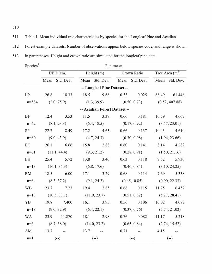
Table 1. Mean individual tree characteristics by species for the Longleaf Pine and Acadian 511

Forest example datasets. Number of observations appear below species code, and range is shown 512

in parentheses. Height and crown ratio are simulated for the longleaf pine data. 513

Species1

Parameter

DBH (cm) Height (m) Crown Ratio Tree Area (m2)

Mean Std. Dev. Mean Std. Dev. Mean Std. Dev. Mean Std. Dev.

-- Longleaf Pine Dataset --

LP 26.8 18.33 18.5 9.66 0.53 0.025 68.49 61.446

n=584 (2.0, 75.9) (1.3, 39.9) (0.50, 0.73) (0.52, 407.88)

-- Acadian Forest Dataset --

BF 12.4 3.53 11.5 3.39 0.66 0.181 10.59 4.667

n=42 (8.1, 23.3) (6.4, 18.5) (0.17, 0.92) (3.57, 23.01)

SP 22.7 8.49 17.2 4.63 0.66 0.137 10.43 4.610

n=60 (9.0, 43.9) (4.7, 24.3) (0.30, 0.98) (1.94, 23.66)

EC 26.1 6.66 15.8 2.88 0.60 0.141 8.14 4.282

n=61 (11.1, 44.4) (9.3, 21.2) (0.28, 0.91) (1.50, 21.16)

EH 25.4 5.72 13.8 3.40 0.63 0.118 9.52 5.930

n=13 (16.1, 35.3) (6.8, 17.6) (0.46, 0.84) (3.10, 24.25)

RM 18.5 6.00 17.1 3.29 0.68 0.114 7.69 5.338

n=64 (8.3, 37.2) (9.1, 24.2) (0.45, 0.85) (0.90, 22.33)

WB 23.7 7.23 19.4 2.85 0.68 0.115 11.75 6.457

n=13 (10.5, 33.1) (11.9, 23.7) (0.51, 0.82) (5.27, 28.41)

YB 19.8 7.400 16.1 3.95 0.56 0.106 10.02 4.087

n=18 (9.0, 32.9) (6.4, 22.1) (0.37, 0.76) (5.74, 21.02)

WA 23.9 11.870 18.1 2.98 0.76 0.082 11.17 5.218

n=6 (8.7, 38.0) (14.0, 23.2) (0.65, 0.84) (2.74, 15.52)

AM 13.7 -- 13.7 -- 0.71 -- 4.15 --

n=1 (--) (--) (--) (--)

1LP = longleaf pine; BF = balsam fir; SP = spruce; EC = eastern cedar; EH = eastern hemlock; 514

RM = red maple; WB = white birch; YB = yellow birch; WA = white ash; and AM = American 515

mountain-ash. 516

517

Table 2. Estimated parameters for the Longleaf Pine and Acadian Forest datasets. 518

Parameter Dataset

Longleaf Pine Acadian Forest

mu 5.7964 0.3054

sigma 4.1094 0.3204

kappa 2.5188 X 10-3

0.3378

density (trees in area) 584 258

x-range {0, 200} {0, 50}

y-range {0, 200} {0, 50}

519

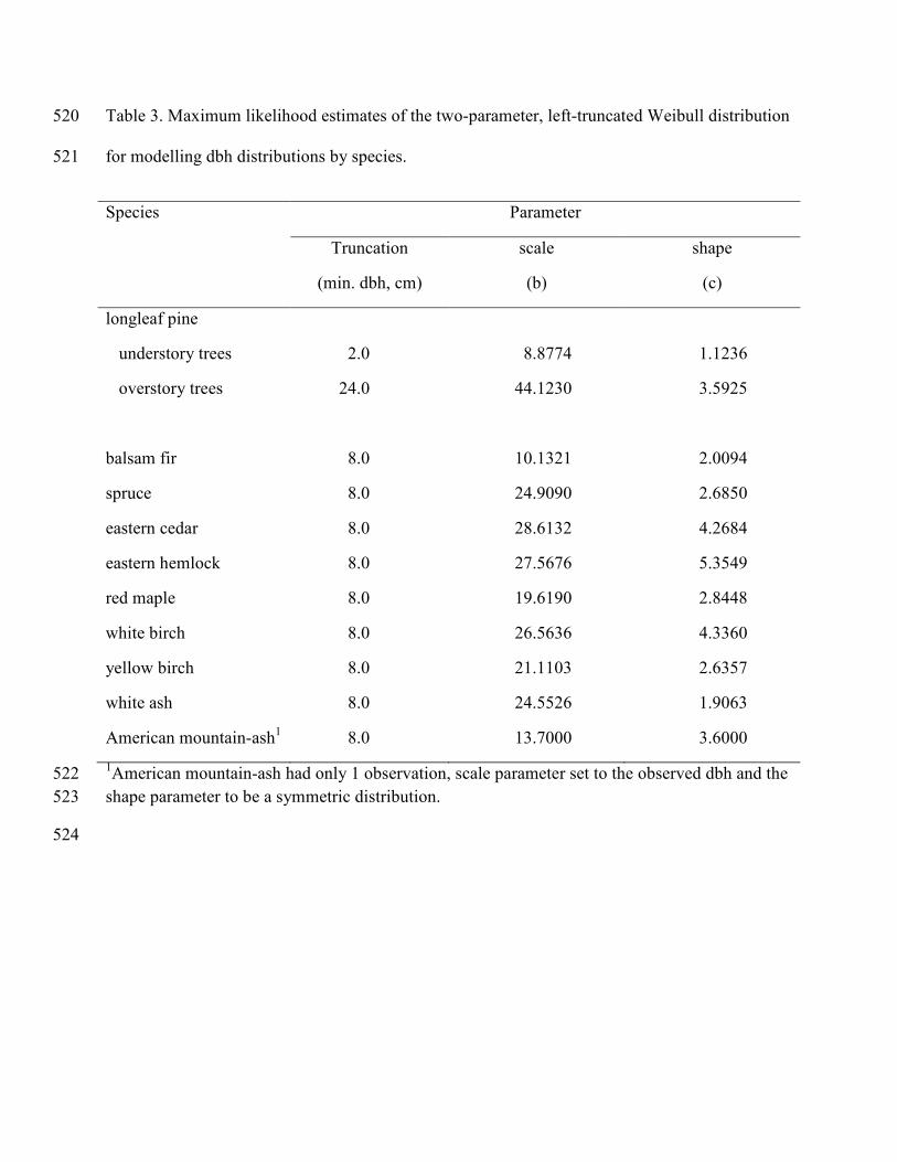
Table 3. Maximum likelihood estimates of the two-parameter, left-truncated Weibull distribution 520

for modelling dbh distributions by species. 521

Species Parameter

Truncation

(min. dbh, cm)

scale

(b)

shape

(c)

longleaf pine

understory trees 2.0 8.8774 1.1236

overstory trees 24.0 44.1230 3.5925

balsam fir 8.0 10.1321 2.0094

spruce 8.0 24.9090 2.6850

eastern cedar 8.0 28.6132 4.2684

eastern hemlock 8.0 27.5676 5.3549

red maple 8.0 19.6190 2.8448

white birch 8.0 26.5636 4.3360

yellow birch 8.0 21.1103 2.6357

white ash 8.0 24.5526 1.9063

American mountain-ash1 8.0 13.7000 3.6000

1American mountain-ash had only 1 observation, scale parameter set to the observed dbh and the 522

shape parameter to be a symmetric distribution. 523

524

Table 4. Maximum likelihood estimates of the three-parameter, reverse Weibull distribution for 525

modelling height distributions by species. 526

Species Parameter

location

(max. ht., m)

scale1

(b)

shape

(c)

longleaf pine

understory trees 22.7 8.3569 2.6615

overstory trees 40.1 25.2362 3.5502

balsam fir 18.6 10.7582 2.0524

spruce 24.4 16.4588 1.5749

eastern cedar 21.3 15.1229 1.9645

eastern hemlock 17.7 13.6660 1.1269

red maple 24.3 16.3058 2.1941

white birch 23.8 19.0692 1.5600

yellow birch 22.2 17.4692 1.4917

white ash 23.3 17.8289 1.3122

American mountain-ash2 14.7 13.7 3.6

1scale parameter defined in terms of height above ground, true scale parameter is height below 527

maximum and is location – scale. 2American mountain-ash only had 1 observation, location was 528

set 1 m above observed value, scale was set to the observed value, and the shape was set to a 529

symmetric distribution. 530

531

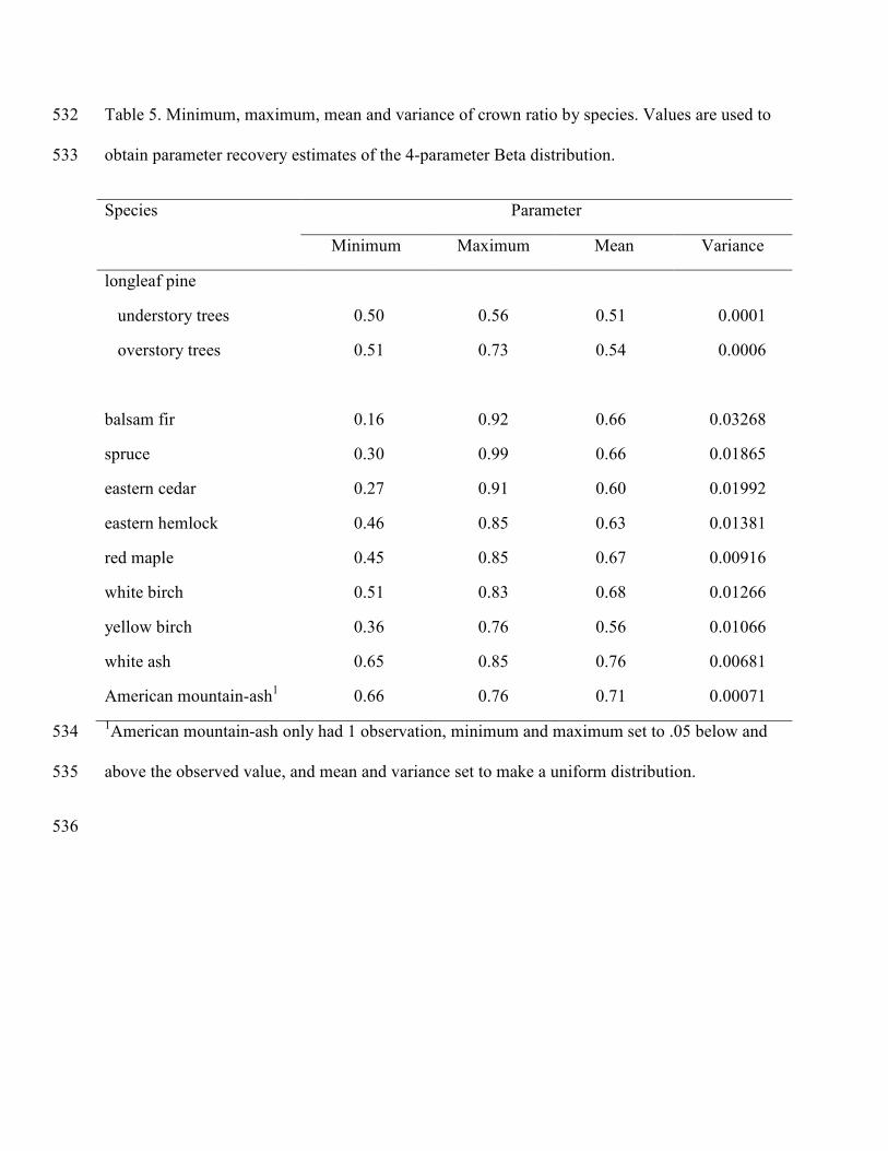
Table 5. Minimum, maximum, mean and variance of crown ratio by species. Values are used to 532

obtain parameter recovery estimates of the 4-parameter Beta distribution. 533

Species Parameter

Minimum Maximum Mean Variance

longleaf pine

understory trees 0.50 0.56 0.51 0.0001

overstory trees 0.51 0.73 0.54 0.0006

balsam fir 0.16 0.92 0.66 0.03268

spruce 0.30 0.99 0.66 0.01865

eastern cedar 0.27 0.91 0.60 0.01992

eastern hemlock 0.46 0.85 0.63 0.01381

red maple 0.45 0.85 0.67 0.00916

white birch 0.51 0.83 0.68 0.01266

yellow birch 0.36 0.76 0.56 0.01066

white ash 0.65 0.85 0.76 0.00681

American mountain-ash1

0.66 0.76 0.71 0.00071

1American mountain-ash only had 1 observation, minimum and maximum set to .05 below and 534

above the observed value, and mean and variance set to make a uniform distribution. 535

536

Table 6. Partial correlations, based on Spearman’s rank correlation, between available tree area, 537

DBH, height and crown ratio for the Longleaf Pine and Acadian Forest datasets. 538

Correlation Dataset

Longleaf Pine Acadian Forest

area – DBH 0.5556 0.1639

area – Height 0.6196 0.1313

area – Crown Ratio 0.7042 -0.1764

DBH – Height 0.9808 0.7118

DBH – Crown Ratio 0.9540 -0.2664

Height – Crown Ratio 0.9849 -0.1564

539

540

Figure Titles 541

Figure 1. Examples of spatial patterns: A) lattice process with no variation; B) a lattice process 542

with multiplicative jittering; C) a homogeneous Thomas process; and D) an inhomogeneous 543

Thomas process. 544

Figure 2. Input windows for the stand structure generator:A) the main menu; B) the lattice spatial 545

model input window; C) the Thomas spatial model input window; D) the species parameter input 546

window; E) the correlation input window; F) the visualization input window; and G) and 547

example Stand Visualization window. 548

Figure 3. Marked spatial correlations for the example datasets: A) longleaf pine dbh; B) Acadian 549

Forest dbh; C) longleaf pine height; D) Acadian Forest height; E) longleaf pine crown ratio; and 550

F) Acadian Forest crown ratio. 551

A) B)

C) D)

Figure 1

A)

B) C)

D)

E)

F)

G)

Figure 2

0.0

0.2

0.4

0.6

0.8

1.0

1.2

r (metres)

m(r

)

0 10 20 30 40 50

A)

0.6

0.7

0.8

0.9

1.0

1.1

1.2

m(r

)

0 2 4 6 8 10 12r (metres)

B)

0.0

0.2

0.4

0.6

0.8

1.0

1.2

r (metres)

m(r

)

0 10 20 30 40 50

C)

0.6

0.7

0.8

0.9

1.0

1.1

1.2

m(r

)

0 2 4 6 8 10 12r (metres)

D)

0.90

0.95

1.00

1.05

1.10

m(r

)

r (metres)0 10 20 30 40 50

E)

0.8

0.9

1.0

1.1

1.2

m(r

)

0 2 4 6 8 10 12r (metres)

F)

Figure 3

TheoreticalObserved1 SimulationMean Simulation