spatially-dependent reactor kinetics and supporting physics validation studies at the high flux
TRANSCRIPT

University of Tennessee, KnoxvilleTrace: Tennessee Research and CreativeExchange
Doctoral Dissertations Graduate School
8-2011
Spatially-Dependent Reactor Kinetics andSupporting Physics Validation Studies at the HighFlux Isotope ReactorDavid [email protected]
This Dissertation is brought to you for free and open access by the Graduate School at Trace: Tennessee Research and Creative Exchange. It has beenaccepted for inclusion in Doctoral Dissertations by an authorized administrator of Trace: Tennessee Research and Creative Exchange. For moreinformation, please contact [email protected].
Recommended CitationChandler, David, "Spatially-Dependent Reactor Kinetics and Supporting Physics Validation Studies at the High Flux Isotope Reactor. "PhD diss., University of Tennessee, 2011.https://trace.tennessee.edu/utk_graddiss/1066

To the Graduate Council:
I am submitting herewith a dissertation written by David Chandler entitled "Spatially-DependentReactor Kinetics and Supporting Physics Validation Studies at the High Flux Isotope Reactor." I haveexamined the final electronic copy of this dissertation for form and content and recommend that it beaccepted in partial fulfillment of the requirements for the degree of Doctor of Philosophy, with a major inNuclear Engineering.
G. Ivan Maldonado, Major Professor
We have read this dissertation and recommend its acceptance:
David H. Cook, Arthur E. Ruggles, Lawrence H. Heilbronn, Rao V. Arimilli
Accepted for the Council:Dixie L. Thompson
Vice Provost and Dean of the Graduate School
(Original signatures are on file with official student records.)

To the Graduate Council:
I am submitting herewith a dissertation written by David Chandler entitled ―Spatially-Dependent
Reactor Kinetics and Supporting Physics Validation Studies at the High Flux Isotope Reactor.‖ I have
examined the final electronic copy of this dissertation for form and content and recommend that it be
accepted in partial fulfillment of the requirements for the degree of Doctor of Philosophy, with a major in
Nuclear Engineering.
G. Ivan Maldonado, Major Professor
We have read this dissertation
and recommend its acceptance:
David H. Cook
Arthur E. Ruggles
Lawrence H. Heilbronn
Rao V. Arimilli
James D. Freels (Courtesy Member)
Accepted for the Council:
Carolyn R. Hodges
Vice Provost and Dean of the Graduate School
(Original signatures are on file with official student records.)
Spatially-Dependent Reactor Kinetics and
Supporting Physics Validation Studies at the
High Flux Isotope Reactor
A Dissertation Presented for the
Doctor of Philosophy
Degree
The University of Tennessee, Knoxville
David Chandler
August 2011

ii
Copyright © 2011 by David Chandler
All rights reserved

iii
DEDICATION
I would like to dedicate this dissertation to my amazing family who has always provided me love,
support, and encouragement. I would like to thank my mother, Sheila Chandler, and my sister, Louise
Pence, who have always believed in me and had the right words to say during all the stressful times. I
would like to thank my girlfriend, Lindsay Sondles, who packed up and moved with me to Tennessee and
has been patient and supportive through my years of research. Finally, and most importantly, I would like
to dedicate this work to my father, Len Chandler, who always believed in me, encouraged me, and taught
me great work ethics.

iv
ACKNOWLEDGEMENTS
This dissertation was made possible by a research contract between the University of Tennessee
Nuclear Engineering Department and the Research Reactors Division of the Oak Ridge National
Laboratory, which is managed by UT-Battelle for the United States Department of Energy.
First and foremost, I would like to express my sincere appreciation to my advising professor, Dr. G.
Ivan Maldonado, and my technical mentor, Mr. R. Trent Primm III, for their time, contributions, and
guidance in my studies. I would like to thank Dr. Maldonado for pursuing and encouraging me to enroll
in graduate school and then continuing to support and advise me. I would like to thank Mr. Primm for
providing me with excellent opportunities at one of the top research facilities in the world and always
making time to assist me in my studies.
I would like to thank the members of my dissertation committee: Dr. James D. Freels, Dr. David H.
Cook, Dr. Arthur E. Ruggles, Dr. Rao V. Arimilli, and Dr. Lawrence H. Heilbronn; for their support and
assistance during my research and dissertation work. I also want to express my sincere gratitude to Dr.
Germina Ilas (ORNL), Dr. Wim Haeck (IRSN in France), and the COMSOL technical support staff who
have helped provide me with the computational tools and information needed to perform much of my
research. I would also like to thank Mr. Randy W. Hobbs, Mr. Larry D. Proctor, Mr. Ron A. Crone, Dr.
Kevin A. Smith, and the rest of the Research Reactors Division for their support and encouragement.
Most importantly I would like to thank my family who has always encouraged me and been there for
me. The most influential people in my life are my parents, Len and Sheila Chandler, who have believed
in me and supported me in all of my life decisions. I would like to thank my sister, Louise Pence, for
always believing in me and being there as both a friend and sister. I would also like to send a special
thank you to my girlfriend, Lindsay Sondles, who started this journey with me and has supported and
believed in me over the years.

v
ABSTRACT
The computational ability to accurately predict the dynamic behavior of a nuclear reactor core in
response to reactivity-induced perturbations is an important subject in the field of reactor physics. Space-
time and point kinetics methodologies were developed for the purpose of studying the transient-induced
behavior of the Oak Ridge National Laboratory (ORNL) High Flux Isotope Reactor’s (HFIR) compact
core. The space-time simulations employed the three-group neutron diffusion equations, which were
solved via the COMSOL partial differential equation coefficient application mode. The point kinetics
equations were solved with the PARET code and the COMSOL ordinary differential equation application
mode. The basic nuclear data were generated by the NEWT and MCNP5 codes and transients initiated by
control cylinder and hydraulic tube rabbit ejections were studied.
The space-time models developed in this research only consider the neutronics aspect of reactor
kinetics, and therefore, do not include fluid flow, heat transfer, or reactivity feedback. The research
presented in this dissertation is the first step towards creating a comprehensive multiphysics methodology
for studying the dynamic behavior of the HFIR core during reactivity-induced perturbations. The results
of this study show that point kinetics is adequate for small perturbations in which the power distribution is
assumed to be time-independent, but space-time methods must be utilized to determine localized effects.
En route to developing the kinetics methodologies, validation studies and methodology updates were
performed to verify the exercise of major neutronic analysis tools at the HFIR. A complex MCNP5
model of HFIR was validated against critical experiment power distribution and effective multiplication
factor data. The ALEPH and VESTA depletion tools were validated against post-irradiation uranium
isotopic mass spectrographic data for three unique full power cycles. A TRITON model was developed
and used to calculate the buildup and reactivity worth of helium-3 in the beryllium reflector, determine
whether discharged beryllium reflectors are at transuranic waste limits for disposal purposes, determine
whether discharged beryllium reflectors can be reclassified from hazard category 1 waste to category 2 or

vi
3 for transportation and storage purposes, and to calculate the curium target rod nuclide inventory
following irradiation in the flux trap.

vii
TABLE of CONTENTS
DEDICATION .......................................................................................................................................................... III
ACKNOWLEDGEMENTS ..................................................................................................................................... IV
ABSTRACT ................................................................................................................................................................ V
LIST OF FIGURES .................................................................................................................................................. XI
LIST OF TABLES ................................................................................................................................................... XV
1 INTRODUCTION .............................................................................................................................................. 1
1.1 ORGANIZATION OF DISSERTATION ........................................................................................................... 1
1.2 MOTIVATION AND GOAL .......................................................................................................................... 3
1.3 LITERATURE REVIEW ............................................................................................................................... 8
1.3.1 HFIR Physics Calculations ............................................................................................................. 9
1.3.2 Current HFIR SAR Methods ......................................................................................................... 10
1.3.3 Point Kinetics Studies at HFIR ..................................................................................................... 11
1.3.4 Codes for Reactor Transient Analysis ........................................................................................... 12
1.3.5 COMSOL Neutronics Modeling .................................................................................................... 12
1.4 BRIEF NUCLEAR BACKGROUND.............................................................................................................. 13
1.4.1 Reactor Physics ............................................................................................................................. 13
1.4.2 Nuclear Reactors .......................................................................................................................... 16
2 DESCRIPTION OF THE HIGH FLUX ISOTOPE REACTOR .................................................................. 20
3 DESCRIPTION OF COMPUTER CODES ................................................................................................... 30
3.1 MCNP5 .................................................................................................................................................. 30
3.2 ORIGEN ................................................................................................................................................ 31
3.3 ALEPH .................................................................................................................................................. 34
3.4 VESTA .................................................................................................................................................. 36
3.5 SCALE ................................................................................................................................................... 37
3.5.1 CSAS ............................................................................................................................................. 38

viii
3.5.2 KENO ............................................................................................................................................ 38
3.5.3 ORIGEN-S..................................................................................................................................... 39
3.5.4 TRITON ......................................................................................................................................... 39
3.5.5 NEWT ............................................................................................................................................ 40
3.6 PARET ................................................................................................................................................... 41
3.7 COMSOL ............................................................................................................................................... 42
4 CRITICAL EXPERIMENT POWER DISTRIBUTIONS ............................................................................ 45
4.1 BACKGROUND OF CRITICAL EXPERIMENTS ............................................................................................ 46
4.2 METHODOLOGY ...................................................................................................................................... 49
4.2.1 HFIRCE-3 HFIR MCNP Model .................................................................................................... 49
4.2.2 HFIRCE-3 MCNP Calculations .................................................................................................... 54
4.3 HFIRCE-3 RESULTS ............................................................................................................................... 57
4.3.1 Clean Core Results........................................................................................................................ 57
4.3.2 Fully Poisoned Results .................................................................................................................. 63
4.4 HFIRCE-3 SUMMARY ............................................................................................................................ 68
5 EXPOSURE-DEPENDENT NUCLIDE INVENTORY ................................................................................ 69
5.1 POST-IRRADIATION DATA ...................................................................................................................... 69
5.2 COMPUTATIONAL MODEL DEVELOPMENT .............................................................................................. 73
5.2.1 HFIR MCNP Model Development ................................................................................................ 75
5.2.2 Computational Model Input Parameters ....................................................................................... 81
5.3 POST-IRRADIATION INVENTORY RESULTS .............................................................................................. 81
5.3.1 Time-Dependent Eigenvalue Results ............................................................................................. 82
5.3.2 Post-Irradiation Uranium Isotopic Results ................................................................................... 84
5.3.3 Fissile and Neutron Poison Nuclide Inventory ............................................................................. 91
5.4 POST-IRRADIATION INVENTORY SUMMARY ........................................................................................... 94
6 BERYLLIUM ACTIVATION IMPACTS ON STARTUP AND REFLECTOR DISPOSAL ................... 96
6.1 BERYLLIUM ACTIVATION EFFECTS ......................................................................................................... 96

ix
6.1.1 Nuclear Transmutations Caused by Neutron Activation ............................................................... 97
6.1.2 Startup Procedure ....................................................................................................................... 101
6.1.3 Beryllium Waste Concerns .......................................................................................................... 102
6.2 COMPUTATIONAL METHODOLOGY ....................................................................................................... 104
6.2.1 Startup Reactivity Effects Methodology ...................................................................................... 105
6.2.2 Waste Classifications Methodology ............................................................................................ 106
6.3 BERYLLIUM ACTIVATION RESULTS ...................................................................................................... 112
6.3.1 Startup Reactivity Effects Results ................................................................................................ 112
6.3.2 Nuclear Waste Classification Results ......................................................................................... 116
6.4 BERYLLIUM ACTIVATION SUMMARY.................................................................................................... 123
7 POST-IRRADIATION CURIUM TARGET ROD INVENTORY ............................................................ 126
7.1 CURIUM TARGET INFORMATION ........................................................................................................... 128
7.2 COMPUTATIONAL METHODOLOGY ....................................................................................................... 131
7.3 CURIUM TARGET RESULTS ................................................................................................................... 133
7.4 CURIUM TARGET SUMMARY ................................................................................................................ 135
8 TWO-DIMENSIONAL BOC STATIC FLUX DISTRIBUTIONS ............................................................. 136
8.1 NEWT MODEL DEVELOPMENT ............................................................................................................ 137
8.2 DERIVATION OF DIFFUSION THEORY .................................................................................................... 141
8.3 COMSOL MODEL DEVELOPMENT ....................................................................................................... 145
8.4 NEWT/COMSOL TWO-GROUP FLUX RESULTS .................................................................................. 150
8.5 TWO-DIMENSIONAL BOC STATIC FLUX DISTRIBUTION SUMMARY ..................................................... 163
9 SPATIALLY-DEPENDENT AND POINT KINETICS .............................................................................. 164
9.1 SPACE-TIME COMPUTATIONAL METHODOLOGY .................................................................................. 165
9.1.1 Eigenvalue Study ......................................................................................................................... 168
9.1.2 Stationary Study .......................................................................................................................... 172
9.1.3 Transient Study ........................................................................................................................... 176
9.1.4 Boundary Conditions .................................................................................................................. 178

x
9.2 POINT KINETICS METHODOLOGY ......................................................................................................... 179
9.2.1 PARET Input Description ........................................................................................................... 184
9.3 RATE TRIP CIRCUIT ANALYSIS ............................................................................................................. 185
9.4 CONTROL CYLINDER EJECTION TRANSIENT ......................................................................................... 188
9.4.1 Control Cylinder Ejection Space-Time Methodology ................................................................. 190
9.4.2 Control Cylinder Ejection Point Kinetics Methodology ............................................................. 194
9.5 BLACK RABBIT EJECTION TRANSIENT .................................................................................................. 195
9.5.1 Black Rabbit Ejection Space-Time Methodology ........................................................................ 198
9.5.2 Black Rabbit Ejection Point Kinetics Methodology .................................................................... 202
9.6 REACTOR KINETICS RESULTS ............................................................................................................... 204
9.6.1 Control Cylinder Ejection Results .............................................................................................. 204
9.6.2 Black Rabbit Ejection Results ..................................................................................................... 211
9.7 REACTOR KINETICS SUMMARY ............................................................................................................ 216
10 SUMMARY OF CONCLUSIONS AND SUGGESTIONS FOR FUTURE WORK ................................. 217
10.1 SUMMARY OF CONCLUSIONS............................................................................................................ 217
10.2 SUGGESTIONS FOR FUTURE WORK ................................................................................................... 220
REFERENCES ........................................................................................................................................................ 223
APPENDICES .......................................................................................................................................................... 236
APPENDIX A – COMSOL PDE DISCRETIZATION METHOD ............................................................................. 236
APPENDIX B - PLUTONIUM-238 PRODUCTION FEASIBILITY STUDY ................................................................ 240
APPENDIX C – ADDITIONAL SPACE-TIME KINETICS FIGURES ......................................................................... 244
APPENDIX D – MCNP, NEWT, AND COMSOL NEUTRONICS ANALYSES ...................................................... 248
VITA ......................................................................................................................................................................... 258

xi
LIST of FIGURES
Figure 2.1. HFIR cross section at the horizontal midplane. ....................................................................... 21
Figure 2.2. HFIR reactor core assembly. ................................................................................................... 22
Figure 2.3. Flux trap and fuel element configuration................................................................................. 22
Figure 2.4. IFE and OFE involute fuel plates. ........................................................................................... 26
Figure 2.5. Outer control plate and inner control cylinder. ........................................................................ 27
Figure 2.6. Permanent beryllium reflector. ................................................................................................ 27
Figure 4.1. Location of foils punched out of removable plates (dimensions in cm). ................................. 48
Figure 4.2. Involute IFE plate. ................................................................................................................... 50
Figure 4.3. Horizontal midplane of HFIRCE-3 as modeled in MCNP. ..................................................... 53
Figure 4.4. (PI + W) flux trap and fuel elements as modeled in MCNP. ................................................... 53
Figure 4.5. Actual versus modeled 235
U concentration of foils in the IFE. ................................................ 55
Figure 4.6. Radial relative power profile at horizontal midplane under clean core conditions. ................ 59
Figure 4.7. Axial relative power profile of foil 1 in IFE under clean core conditions. .............................. 59
Figure 4.8. Axial relative power profile of foil 4 in IFE under clean core conditions. .............................. 60
Figure 4.9. Axial relative power profile of foil 6 in IFE under clean core conditions. .............................. 60
Figure 4.10. Axial relative power profile of foil 1 in OFE under clean core conditions. .......................... 61
Figure 4.11. Axial relative power profile of foil 4 in OFE under clean core conditions. .......................... 61
Figure 4.12. Axial relative power profile of foil 6 in OFE under clean core conditions. .......................... 62
Figure 4.13. Radial relative power profile at horizontal midplane under fully poisoned core conditions. 64
Figure 4.14. Axial relative power profile of foil 1 in IFE under fully poisoned core conditions. ............. 65
Figure 4.15. Axial relative power profile of foil 4 in IFE under fully poisoned core conditions. ............. 65
Figure 4.16. Axial relative power profile of foil 6 in IFE under fully poisoned core conditions. ............. 66
Figure 4.17. Axial relative power profile of foil 1 in OFE under fully poisoned core conditions. ............ 66

xii
Figure 4.18. Axial relative power profile of foil 4 in OFE under fully poisoned core conditions. ............ 67
Figure 4.19. Axial relative power profile of foil 6 in OFE under fully poisoned core conditions. ............ 67
Figure 5.1. Axial and radial locations of burnup specimens (cm). ............................................................ 71
Figure 5.2. MCNP as modeled locations of specimens in IFE (left) and OFE (right). .............................. 77
Figure 5.3. Cross section of HFIR MCNP model at the horizontal midplane. .......................................... 79
Figure 5.4. X-Z cross section of HFIR MCNP model. .............................................................................. 79
Figure 5.5. Control element and keff curve for cycle 4. ............................................................................ 83
Figure 5.6. Control element and keff curve for cycle 16. .......................................................................... 83
Figure 5.7. Control element and keff curve for cycle 35. .......................................................................... 84
Figure 5.8. Cycle 4 OFE post-irradiation 234
U atomic percent. ................................................................. 85
Figure 5.9. Cycle 4 OFE post-irradiation 235
U atomic percent. ................................................................. 86
Figure 5.10. Cycle 4 OFE post-irradiation 236
U atomic percent. ............................................................... 86
Figure 5.11. Cycle 4 OFE post-irradiation 238
U atomic percent. ............................................................... 87
Figure 5.12. Cycle 16 OFE post-irradiation 234
U atomic percent. ............................................................. 87
Figure 5.13. Cycle 16 OFE post-irradiation 235
U atomic percent. ............................................................. 88
Figure 5.14. Cycle 16 OFE post-irradiation 236
U atomic percent. ............................................................. 88
Figure 5.15. Cycle 16 OFE post-irradiation 238
U atomic percent. ............................................................. 89
Figure 5.16. Cycle 35 IFE post-irradiation 234
U atomic percent. ............................................................... 89
Figure 5.17. Cycle 35 IFE post-irradiation 235
U atomic percent. ............................................................... 90
Figure 5.18. Cycle 35 IFE post-irradiation 236
U atomic percent. ............................................................... 90
Figure 5.19. Cycle 35 IFE post-irradiation 238
U atomic percent. ............................................................... 91
Figure 5.20. 235
U depletion and 239
Pu buildup as a function of exposure for HFIR cycle 16. ................... 92
Figure 5.21. 135
Xe and 149
Sm buildup as a function of exposure for HFIR cycle 16. ................................ 93
Figure 5.22. 10
B inventory as a function of exposure for HFIR cycle 16. ................................................. 94
Figure 6.1. Transmutation path leading to poison and tritium buildup in the beryllium reflector. ............ 99

xiii
Figure 6.2. Transmutation path for transuranic isotope production [83]. ................................................ 100
Figure 6.3. Isometric view of the HFIR KENO model. ........................................................................... 105
Figure 6.4. SCALE and time-dependent ALEPH/MCNP flux comparisons. .......................................... 108
Figure 6.5. Poison and gas buildup in the beryllium reflector resulting from neutron activation. .......... 113
Figure 6.6. Comparison of current procedure and newly derived 3He poison effect estimates. .............. 115
Figure 6.7. Comparison of current and proposed ESCCEP methodologies against ASCCEP data. ........ 115
Figure 6.8. TRU waste inventory in beryllium reflector regions following discharge. ........................... 117
Figure 6.9. TRU waste inventory in PB3 following discharge. ............................................................... 118
Figure 6.10. June 2010 radionuclide curie levels in PB3 as calculated in TRITON (left), ORIGEN-S best
estimate (middle), and ORIGEN-S conservative (right). .......................................................................... 119
Figure 6.11. Total radioactivity in RB and SPB beryllium and aluminum regions. ................................ 121
Figure 6.12. Major RB and SPB aluminum region radionuclides. .......................................................... 123
Figure 7.1. Flux trap loading summary (407 – 418 are boxed in and are the focus of this study). .......... 127
Figure 7.2. Illustration of the flux trap target positions. .......................................................................... 129
Figure 7.3. Illustration of flux trap target region as modeled in KENO. ................................................. 132
Figure 7.4. KENO and validated MCNP axially averaged flux comparison. .......................................... 133
Figure 7.5. Calculated time-dependent 252
Cf and 249
Bk inventories. ........................................................ 134
Figure 8.1. Schematic representation of NEWT and COMSOL models. ................................................ 138
Figure 8.2. Grid structure and material placement in NEWT model. ...................................................... 140
Figure 8.3. Diffusion theory estimate of the extrapolation distance. ....................................................... 144
Figure 8.4. COMSOL geometry drawing of HFIR. ................................................................................. 146
Figure 8.5. NEWT half core thermal neutron flux distribution. .............................................................. 155
Figure 8.6. NEWT half core fast neutron flux distribution. ..................................................................... 156
Figure 8.7. COMSOL half core thermal neutron flux distribution. ......................................................... 157
Figure 8.8. COMSOL half core fast neutron flux distribution. ................................................................ 158

xiv
Figure 8.9. Thermal (middle) and fast (right) flux in the flux trap (h=60.96cm, r=6.4cm). .................... 159
Figure 8.10. Thermal (middle) and fast (right) flux in the fuel regions (active fuel h=50.8cm). ............ 159
Figure 8.11. Thermal (left) and fast (right) flux in the control elements (h=102cm, w=0.635cm). ........ 160
Figure 8.12. Thermal (left) and fast (right) flux in the beryllium reflector (h=60.96cm, w=30.80cm). .. 160
Figure 8.13. Normalized two-group flux profiles. ................................................................................... 161
Figure 8.14. COMSOL mesh quality (mesh refinement 0 on left, mesh refinement 5 on right). ............ 162
Figure 8.15. Thermal flux (E < 3 eV) contour plots during gadolinium rabbit ejection. ......................... 162
Figure 9.1. Neutron flux PDE boundary conditions. ............................................................................... 179
Figure 9.2. Rate circuit model. ................................................................................................................. 185
Figure 9.3. Control element geometry and interface definitions. ............................................................ 192
Figure 9.4. Mesh-dependent interface property interpolation (mapped mesh on the left and triangular
mesh on the right) ..................................................................................................................................... 194
Figure 9.5. X-ray image of black rabbit RX120R. ................................................................................... 198
Figure 9.6. Geometry used in black rabbit ejection analysis. .................................................................. 199
Figure 9.7. Hydraulic tube axially-dependent property definition. .......................................................... 201
Figure 9.8. Rabbit stack configuration and axial flux profile. ................................................................. 203
Figure 9.9. Space-time calculated reactor power during control cylinder ejection transient. .................. 207
Figure 9.10. Space-time control element movement during control cylinder ejection transient. ............ 208
Figure 9.11. Space-time power distribution and control element movement during control cylinder
ejection transient. ...................................................................................................................................... 209
Figure 9.12. Comparison of control cylinder ejection space-time and point kinetics results. ................. 210
Figure 9.13. 12 MW run 1 ejection power curve, 3.81 cm long Gd cylinder. ......................................... 212
Figure 9.14. 12 MW run 2 ejection power curve, 3.81 cm long Gd cylinder. ......................................... 213
Figure 9.15. 12 MW run 3 ejection power curve, 3.81 cm long Gd cylinder. ......................................... 214
Figure 9.16. 85 MW ejection power curve, 2.54 cm long Gd cylinder.................................................... 215
xv
LIST of TABLES
Table 2.1. Summary of HFIR characteristics. ............................................................................................ 29
Table 2.2. Radial boundaries of core components ..................................................................................... 29
Table 4.1. Summary of critical experiments. ............................................................................................. 46
Table 4.2. MCNP radial boundaries of reactor assembly. ......................................................................... 49
Table 4.3. Fuel radial region boundaries. ................................................................................................... 51
Table 4.4. Summary of cycle 400 production core and HFIRCE-3. .......................................................... 52
Table 4.5. Percent difference of 235
U modeled in IFE................................................................................ 56
Table 4.6. Percent difference of 235
U modeled in OFE. ............................................................................. 56
Table 4.7. Effective multiplication factors for clean core conditions. ....................................................... 57
Table 4.8. Effective multiplication factors for poisoned core conditions. ................................................. 63
Table 5.1. Summary of fuel elements analyzed. ........................................................................................ 72
Table 5.2. Radial dimensions of major HFIR model regions. ................................................................... 75
Table 6.1. Irradiation history input for PB3 ORIGEN-S calculations. .................................................... 111
Table 6.2. Irradiation history input for RB and SPB ORIGEN-S calculations. ....................................... 112
Table 6.3. PB3 post-discharge radionuclides (Ci) (largest from TRITON or ORIGEN-S). .................... 120
Table 6.4. Representative RB post-discharge radionuclides (Ci) (ORIGEN-S). ..................................... 122
Table 6.5. Representative SPB post-discharge radionuclides (Ci) (ORIGEN-S). ................................... 122
Table 7.1. Irradiation history of target rods. ............................................................................................ 129
Table 7.2. Initial curium targets actinide loading (atoms/barn-cm). ........................................................ 130
Table 7.3. Calculated end-of-life transuranic nuclide inventory in curium targets. ................................. 134
Table 8.1. Geometric and material descriptions of NEWT/COMSOL model regions. ........................... 139
Table 8.2. Automatic mesh refinement statistics/parameters. .................................................................. 161
Table 9.1. Three-group energy structure. ................................................................................................. 168

xvi
Table 9.2. Conditions used to define axially-dependent properties. ........................................................ 193
Table 9.3. Isotopic composition of gadolinium. ...................................................................................... 197
Table 9.4. Summary of space-time control cylinder ejection transient calculation. ................................ 206
1
1 Introduction
Chapter 1 presents a brief background on and an introduction to the research performed and
documented in this dissertation. The subsections of this chapter discuss the content and organization of
this dissertation, the motivation behind the research performed, a brief background on nuclear energy and
nuclear reactor physics, and a literature review on documented studies related to the research presented in
this dissertation.
1.1 Organization of Dissertation
This dissertation is divided and organized into several chapters including this introductory chapter.
Chapter 1 presents background information on the motivation behind the studies presented in this
dissertation, previous documented studies related to this dissertation, and nuclear engineering. Chapter 2
discusses the necessary background information on the High Flux Isotope Reactor (HFIR) needed to
understand the body of this dissertation and includes when and why the HFIR was constructed and
physical descriptions of the reactor. Descriptions of the pertinent computational tools used throughout
this dissertation are presented in Chapter 3.
Chapters 4 through 9 document the research performed in this dissertation and are organized such that
each chapter builds on the previous chapters. Chapters 4 through 7 present studies validating some of the
computational tools and neutron cross section data against HFIR specific experiments. These tools and
data are required for generating essential input for the computational tools used in the research
documented in Chapters 8 and 9.
The Monte Carlo transport code, MCNP, and the continuous energy ENDF/B-VI.8 neutron cross
section library are validated for the HFIR core in Chapter 4 with power distribution and effective
multiplicative factor data from critical experiments. The studies presented in this chapter have previously
been published in [1], [2], and [3].

2
Two Monte Carlo-based depletions tools, ALEPH and VESTA, and the continuous energy ENDF/B-
VI.8 and ENDF/B-VII neutron cross section libraries are validated for the HFIR core in Chapter 5 with
spatially-dependent post-irradiation uranium isotopic atomic percentages. The analyses presented in this
chapter have been published in [4], [5], [6], and [7].
Chapter 6 presents the development of a three-dimensional SCALE model of HFIR and serves to
validate the model as well as the ENDF/B-VII 238-group neutron cross section library, specifically for
beryllium activation calculations; thus, validating the cross sections and fluxes present in the beryllium
reflector. This chapter discusses the effects neutron activation on the beryllium reflector has on the
approach to critical at startup and the impact it has on disposing of the reflector. The various studies
presented in this chapter have been published in [8], [9], [10], [11], and [12].
Chapter 7 discusses a validation study performed with the model developed in Chapter 6 to calculate
the post-irradiation 252
Cf and 249
Bk inventory in curium target rods irradiated in the flux trap of HFIR.
Thus, the SCALE model and the ENDF/B-VII 238-group neutron cross section library are validated for
calculating the cross sections and fluxes in curium targets located in the flux trap of HFIR. The study
documented in Chapter 7 is published in [13].
A two-dimensional, two-group diffusion theory model of HFIR was developed in COMSOL and
documented in Chapter 8 to study the spatially-dependent, beginning-of-cycle fast and thermal neutron
fluxes. This study was the first step along the path to implementing two- and (possibly) three-
dimensional models of HFIR in COMSOL for the purpose of studying the spatial dependence of
transient-induced behavior in the reactor core. Parts of this chapter are presented in [14] and [15].
The research documented in Chapter 9 is the primary focus of this dissertation. COMSOL-based
time- and space-dependent, three-group, neutron kinetics models of HFIR are discussed. The purpose of
this research is to develop a methodology, which will be used to study the power distribution in the
reactor core during reactivity-induced transients that are introduced nonuniformly throughout the core.
The COMSOL and PARET codes are also used in this chapter to develop new reactor point kinetics

3
methodologies. The solutions calculated via the space-dependent kinetics and the point kinetics
methodologies are compared.
1.2 Motivation and Goal
Under the sponsorship of the U. S. Department of Energy’s (DOE) National Nuclear Security
Administration (NNSA), staff members at the Oak Ridge National Laboratory (ORNL) have been
conducting studies to determine whether the High Flux Isotope Reactor can be converted from high
enriched uranium (HEU) fuel to low enriched uranium (LEU) fuel. Converting domestic and
international civilian research reactors and isotope production facilities from the use of weapons of mass
destruction (WMD) usable HEU fuel to LEU is one of the three subprograms of the Global Threat
Reduction Initiative (GTRI) to deny terrorists access to nuclear and radiological materials [16]. The
Reduced Enrichment for Research and Test Reactors (RERTR) Program [17] and the National
Organization of Test, Research, and Training Reactors (TRTR) [18] were formed to promote
collaboration between research reactors and RERTR was setup specifically to support the conversion.
Research reactors are designed for specific scientific missions and the mission of HFIR for example is
to produce the highest achievable steady state neutron currents to experiment facilities for neutron
scattering experiments, isotope production, materials irradiation, and neutron activation analysis. The
GTRI/RERTR Program has defined goals for the replacement of HEU in research reactors and some of
the key objectives include:
1. Ensure that the ability of the reactor to perform its scientific mission is not significantly
diminished.
2. Work to ensure that an LEU fuel alternative is provided that maintains a similar service lifetime
for the fuel assembly.
4
3. Ensure that conversion to a suitable LEU fuel can be achieved without requiring major changes in
reactor structures or equipment.
4. Determine, to the extent possible, that the overall costs associated with conversion to LEU fuel
does not increase the annual operating expenditure for the owner/operator.
5. Demonstrate that the conversion and subsequent operation can be accomplished safely and the
LEU fuel meets safety requirements.
6. Work in concert with the fuel return programs to coordinate the schedule of HEU fuel removal
with the LEU fuel delivery to initiate conversion.
7. For more rapid or immediate conversions, the owner/operator may be compensated for the unused
service lifetime of the repatriated HEU fuel.
Thus, after conversion, HFIR must be able to safely operate while maintaining reactor performance
and a similar fuel cycle length. The reactor performance must not be diminished, and therefore, the
neutron flux (magnitude and spectra) at the experiment facilities must not be diminished and must be
maintained for the duration of a typical HEU fuel cycle length in calendar time.
The HEU fuel currently loaded in HFIR is approximately 93 percent by weight 235
U/U in the form of
U3O8-Al (a blend of ceramic and metallic powders) and the proposed LEU fuel will be enriched to 20
percent by weight 235
U/U in the form of U-10Mo, a uranium metal alloyed with molybdenum with the Mo
composing 10 percent by weight of the mixture. The fresh core uranium loading will increase from 10.1
kg for HEU fuel to about 125 kg for LEU fuel. Due to self shielding effects introduced by the large
concentration of 238
U, the critical mass of 235
U will be increased from 9.4 kg (HEU fuel) to 25 kg (LEU
fuel) and the densest fuel available will be needed [19]. The denser LEU fuel will also cause the reactor
power to be increased from 85 MWth to 100 MWth in order to maintain the neutron flux at the experiment
facilities. Increasing the power while maintaining the same end-of-cycle fuel burnup (MWd) shortens the
fuel cycle length (days), and therefore, the discharged fuel burnup must be increased by a ratio of 100/85
to maintain the same cycle length [20].

5
The current HEU core was designed based on experiments, calculations, and expert-based opinions.
However, today, experiments are very expensive and critical experiment facilities in existence at the time
HFIR was built are no longer available and replacement facilities have not been constructed. With
current advances in computational power, fuel design studies have become more reliant on performing
calculations via validated computational-based simulations and methods. Numerical analysis programs
are available and are able to accurately predict pertinent physics parameters, and are thus utilized for
studies such as converting to LEU fuel. Additionally, utilizing computationally-based programs is useful
and economical for safety assessments in which it is undesirable to experimentally determine the transient
behavior of the reactor, and similarly, to minimize the risk of failure of a specimen proposed for
irradiation and the consequences of such a failure should it occur. For design and safety purposes, it is
vital to validate computer codes before relying on their results, which is ideally carried out by comparing
computational simulations against actual operational or experimental measurements, as available.
The purpose of the studies presented in this dissertation is to develop and validate new methodologies
using modern, state-of-the-art computational tools to perform physics studies on the HFIR. The
methodologies described in these studies were developed and validated for HEU fuel and have been or
will be adopted for LEU fuel studies. Currently, no LEU fuel experimental physics data exists, and thus,
it is important to first validate these methods against the existing HEU fuel experimentally measured
results before applying them to LEU fuel studies.
It is very important to develop new methodologies based on current tools because programs of the
past often go unmaintained, become unsupported, and grow incompatible with current software. The
latest programs are often newer versions of the original program that implement more efficient and
accurate numerical methods and better (nuclear) data. The validation studies presented here make use of
Monte Carlo codes and detailed three-dimensional geometry. Diffusion theory-based models are
developed in this dissertation and are applied to some of the time-dependent analyses because diffusion

6
theory requires much less computational time than Monte Carlo codes and have the ability to calculate
fluxes at mesh intervals inside small regions.
Validating codes against experimental data and other computer codes is very important to ensure that
the calculations are accurate, to determine any computational biases, and to establish the code’s range of
applicability. Pertinent sources of neutronics measurements that are applicable to validating reactor
physics codes include, but are not limited to: power/flux distributions in the reactor core, spent fuel
isotopic inventories and distributions within the core, decay heat generation rates, criticality (keff) data,
fuel cycle length, and irradiated target isotopic compositions.
Critical experiment data including effective multiplication factors and power distributions at
beginning-of-cycle and end-of-cycle (simulated with boron poison in coolant to represent fission products
and fuel burnup) was used to validate a detailed MCNP5 input. MCNP5 coupled with ORIGEN 2.2 via
the ALEPH and VESTA computer codes were validated with keff, cycle length, and spatially-dependent
end-of-cycle uranium isotopic inventory data obtained from three HFIR cores that were irradiated in the
mid to late 1960s. The SCALE sequence TRITON including the KENO and ORIGEN-S codes was used
to determine the nuclide inventory in discharged curium targets irradiated in the flux trap of HFIR as well
as discharged beryllium reflectors. The calculated 252
Cf and 248
Bk inventory in the discharged curium
targets were compared to dissolver solution measurements. The buildup of neutron absorbers; 3He and
6Li; and gases;
3H,
3He, and
4He; in the beryllium reflector were studied and the
3He buildup was used to
develop a new methodology to predict its reactivity impact on the beginning-of-cycle control element
position.
The HEU validation studies herein described partially support the use of these tools for LEU
applications, so to ensure that the ability of the LEU fuelled HFIR to perform its scientific mission is not
diminished, to ensure that the LEU fuel alternative maintains a similar cycle length, and to better
7
understand the nuclear physics characteristics of the LEU fuel. The motivation behind developing a time-
and spatially-dependent reactor kinetics methodology is derived from:
developing a new HEU-based reactivity-induced transient modeling methodology to be
applied to the LEU fuel in order to ensure the new HFIR fuel meets safety requirements,
eliminating the assumptions associated with the current methodology of reactor point (zero-
dimensional) kinetics,
eliminating the conservatisms applied to the current methodology,
ongoing efforts to update the HFIR thermal-hydraulic and structural methods,
and the recent interest and advances in spatially-dependent reactor kinetics coupled with
advances in computational power and numerical methods.
A spatially-dependent kinetics study of HFIR has been postulated in the past in order to confirm the
point kinetics assumption, but has never been performed. The main objective of this dissertation is to
develop a space-time kinetics methodology for the HFIR. The current methodology used for studying
HFIR transients and limitations to the point kinetics approach are discussed in detail in the following
paragraphs.
Point kinetics has been widely used in the nuclear industry to predict the time-dependent behavior of
nuclear reactors. The major assumption associated with point kinetics is that the fundamental flux mode
dominates the transient. During steady state operations, a nuclear reactor is critical and operating in the
fundamental mode. Under the point kinetics assumption, the properties of the reactor are rapidly changed
uniformly throughout the system and the flux remains in the fundamental mode of the original,
unperturbed system when reactivity is introduced to the reactor and the effective multiplication factor is
no longer unity. The current methodology assumes that the higher harmonics die out faster than the
reactivity change that is imposed on the system, and thus, the fundamental mode is achieved, which may
not be true [21]. However, HFIR transients are not induced by uniform reactivity changes, and thus, the

8
properties of the reactor are not changed uniformly. A couple of examples of reactivity additions that
would not induce uniform reactivity changes include ejecting a europium lined rabbit from the hydraulic
tube (center of core, moving upwards) and a control cylinder ejection (outside of core, moving away from
the core in the axial direction. The spatial effects introduced by reactivity-induced perturbations in HFIR
are the aim of the space-time kinetics study presented in this dissertation.
COMSOL, a finite element-based tool, has recently been adopted at HFIR for performing thermal-
hydraulic analyses and is being used to determine whether the LEU fuel will need to be axially graded to
satisfy thermal requirements. Three-dimensional models of HFIR fuel plates have been developed such
that heat transfer can be modeled in all three dimensions, which is an improvement over current one-
dimensional models that only include heat transfer through the plate (no axial or span-wise conduction)
[22]. This study has proven to be valuable and is another driver behind developing a COMSOL-based
space-time kinetics model.
1.3 Literature Review
This purpose of the section is to collect and summarize information relevant to this dissertation topic;
studying the spatially-dependent effects caused by reactivity-induced perturbations in the HFIR core.
This section is broken into a few subsections to include a brief documentation on the 1) core physics
calculations, 2) methods used in HFIR’s Safety Analysis Report (SAR) to predict the core’s response to
possible transients, 3) previous studies at HFIR pertaining to reactivity-induced transients, 4) spatially-
dependent commercial transient codes used for power reactors, and 5) published studies involving
COMSOL neutronics calculations.
9
1.3.1 HFIR Physics Calculations
The HFIR core physics validation studies were a continuation of the work performed by N. Xoubi
[23]. Xoubi performed his dissertation via a contract between the University of Cincinnati and the
Research Reactors Division, ORNL, and published his research in November 2005. Xoubi modified a
previous MCNP model of HFIR and validated it against HFIR fuel cycle number 400 [24]. Xoubi’s main
research goal made use of this HFIR MCNP model and ALEPH, a generic depletion tool, to study the
behavior of the predicted, time-dependent effective eigenvalue, i.e., eigenvalue drift.
Xoubi’s cycle 400 model was used throughout this dissertation to develop new and original Monte
Carlo-based methodologies to predict the time- and spatially-dependent power distribution profiles and
uranium isotopic atomic percent distributions. New SCALE models, KENO V.a and KENO-VI, of HFIR
were developed and utilized in this dissertation and were created based on the material compositions and
geometrical boundaries used in the cycle 400 model. These models were used to develop new and
original methodologies to predict the reactivity effect neutron poisons (3He and
6Li) have on starting
HFIR following long outages, predicting the post-irradiation and post-discharge radionuclide inventory in
beryllium reflectors, and the post-irradiation nuclide inventory in curium target rods irradiated in the flux
trap target region.
G. Ilas has also performed a variety of core physics studies at HFIR including developing a VESTA
model of HFIR for depletion calculations [25] and an LEU-based NEWT model for calculating
microscopic cross sections for insertion into VENTURE inputs [26]. Modifications were applied to Ilas’
VESTA model in this dissertation in order to compare against the calculations described in the previous
paragraph as well as to develop a new methodology for predicting the 238
Pu production rate in 237
Np
targets to be irradiated in the beryllium reflector. The LEU-based NEWT model was appropriately
modified for HEU-based calculations to generate macroscopic cross sections needed to solve the diffusion
theory equations coded into the HFIR COMSOL models developed in this dissertation.

10
R. T. Primm, III performed a variety of core physics studies including calculating time-dependent
power distributions and effective eigenvalues in the early 1990s [27]. These studies utilized two-
dimensional diffusion theory and few group ENDF/B-V neutron cross section data. The majority of the
core physics studies presented in this document make use of Monte Carlo transport codes, which allow
for a more detailed three-dimensional HFIR geometry to be modeled. Also, a combination of continuous
energy nuclear data and 238-group nuclear data are utilized.
1.3.2 Current HFIR SAR Methods
The current method used to study HFIR reactivity-induced transients makes use of the RELAP5
thermal-hydraulic solver coupled to a stand-alone reactor point kinetics solver [28]. Although RELAP5
has a self-contained point kinetics solver built into it, a replacement point kinetics solver was developed
by Dr. J. D. Freels, ORNL, and linked to the thermal-hydraulics solver. The RELAP5 input is executed
for a user-defined amount of time (typically 100 seconds) in order to reach steady state conditions. A
restart is performed on the RELAP5 code coupled to the point kinetics solver such that a reactivity
induced transient can be modeled. The point kinetics input utilizes six-groups of delayed neutron
precursors and conservative temperature and voiding coefficients. RELAP5 is used to calculate the
temperatures and void fractions needed for input in the feedback equations and the point kinetics
equations make use of the reactivity and delayed neutron data to calculate the power feedback. The major
assumptions in this method include performing one-dimensional RELAP5 calculations and zero-
dimensional point kinetics calculations to study the reactor power during a reactivity excursion.

11
1.3.3 Point Kinetics Studies at HFIR
A point kinetics model of the HFIR core was developed in PARET, a computer code that couples
point kinetics to one-dimensional heat transfer and fluid equations, in 2009 [29]. This input models the
HFIR core (fuel, clad, and coolant) as 17 radial ―core‖ regions (8 regions for the inner fuel element and 9
regions for the outer fuel element) and 19 axial regions such that a spatial power distribution is modeled
in the ―nested tube in slab‖ geometry. Each ―core‖ has its own power generation and coolant flow rate
and represents a single fuel plate (not a single HFIR involute fuel plate). The point kinetics equations are
solved for each ―core‖ with six delayed neutron precursor groups and feedback from fuel temperature,
water temperature, and voiding. The resulting power from each of the ―cores‖ are summed together to
determine the total core power as a function of time. This input was used to predict the power and
reactivity introduced by a decrease in the primary flow rate with HFIR loaded with HEU and LEU fuel.
This study showed that a decrease in the primary flow rate is more severe for the HEU loaded core in
comparison to the LEU fuelled core.
In the early 1990s, a coupled neutronics (point kinetics) and core thermal hydraulics model was
developed by T. Sofu for the purpose of studying possible reactivity insertion accidents at HFIR [30].
The point kinetics equations utilized up to six groups of delayed neutron precursors and feedback from
temperature and voiding. This model utilized one-dimensional, non-homogenous, equilibrium two-phase
flow and heat transfer with the provision for subcooled boiling in the coolant channels and spatially-
averaged, one-dimensional heat conduction for the fuel plates. To solve these coupled equations, a direct
numerical solution of the multiple point difference approximation to the equations representing the core
dynamics model were used in an implicit fashion [30]. This model was used to investigate accidents
involving withdrawal of the control elements, over cooling the core region (i.e., a pump start in a cold idle
heat exchanger loop), and voids in the target region (i.e., flow blockage, etc.) for both nominal conditions
(nominal power density, average heat flux, zero manufacturing tolerances, no uncertainties in the
operational characteristics, etc.) and hot-spot conditions (reduced coolant channel width and flow;

12
uncertainties in operating conditions, power density distributions, heat transfer characteristics, fuel
loading; etc.). In Section 9.2 of [30], T. Sofu recommends that a space-kinetics approach may be needed
to address the space-independent point kinetics approximation.
Studies of HFIR transients by means of point kinetics equations have been the focus of several other
published documents, some of which are internal to the Research Reactors Division, [31] - [37]. These
are not discussed in detail in this section, but a few of these studies, [33] - [36], studied space-
dependency by modeling the reactor as 2 to 4 zero-dimensional systems, i.e., four point kinetics analyses
summed together. To date, there has been no attempt at HFIR to study the spatially-dependent core flux
distribution during a reactivity-induced transient, which is the focus of this dissertation.
1.3.4 Codes for Reactor Transient Analysis
The existing computer codes, [38] - [44], that are used for modeling reactivity-induced transients are,
in general, developed for commercial power reactors with geometries and operating conditions
significantly different from HFIR. Thus, these types of codes have a limited range of applicability for
research reactors such as HFIR. HFIR is unique because of its compact core design (height = 2 ft, outer
radius = 8.5 in), which is composed of 540 involute-shaped, HEU (93 % 235
U/U) loaded fuel plates. In
comparison, a typical commercial light water reactor is composed of approximately 50000 fuel rods that
are about 12 feet in length and filled with fuel pellets enriched to 2 - 5 percent in 235
U/U.
1.3.5 COMSOL Neutronics Modeling
G. Gomes created a two-dimensional, two-group, two-region (fuel + reflector) diffusion theory model
of a single lattice benchmark problem and compared his results against the Reactor Fuelling Simulation
Program in [45]. V. Memoli, et. al., developed a two-dimensional, two-group, two-region (liquid fuel and
graphite reflector) diffusion theory model of a single Molten Salt Reactor (MSR) core channel and

13
compared his results to SCALE and MCNP in [46]. Both of these studies utilized partial regions of
power reactor cores whereas this dissertation focuses on a compact research reactor core. Also, these two
studies focus on static analyses of LEU-type fuel, solid and liquid, whereas this dissertation presents static
and time-dependent analyses of a HEU fuelled core.
1.4 Brief Nuclear Background
This section serves to present a brief background on nuclear energy and is subdivided into two
sections. Section 1.4.1 presents some of the pertinent nuclear reactor physics concepts used and further
discussed throughout this dissertation. Section 1.4.2 discusses a brief background on nuclear energy and
the role of nuclear reactors today.
1.4.1 Reactor Physics
Nuclear energy is produced by means of nuclear fission reactions. A fission reaction occurs when a
neutron bombards the nucleus of an atom, typically fissile heavy isotopes like 235
U, which subsequently
forms an excited nucleus and splits into smaller elements, called fission fragments, freeing neutrons and
gamma rays, and thus, releasing energy. In a typical 235
U fuelled reactor, 2 to 3 neutrons are freed and
approximately 200 MeV of energy is released following a fission event. The source of energy is
produced from the mass conversion and most of it is released as kinetic energy associated with the fission
fragments. An example of the fission process is shown in Equation 1.1. The principle of conservation of
mass can be used to determine the energy yield from the reaction defined in Equation 1.1.
Equation 1.1
14
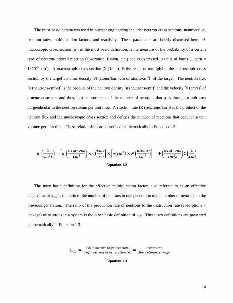
The most basic parameters used in nuclear engineering include: neutron cross sections, neutron flux,
reaction rates, multiplication factors, and reactivity. These parameters are briefly discussed here. A
microscopic cross section (σ), in the most basic definition, is the measure of the probability of a certain
type of neutron-induced reaction (absorption, fission, etc.) and is expressed in units of barns (1 barn =
1x10-24
cm2). A macroscopic cross section [Σ (1/cm)] is the result of multiplying the microscopic cross
section by the target’s atomic density [N (atoms/barn-cm or atoms/cm3)] of the target. The neutron flux
[ϕ (neutrons/cm2-s)] is the product of the neutron density [n (neutrons/cm
3)] and the velocity [v (cm/s)] of
a neutron stream, and thus, is a measurement of the number of neutrons that pass through a unit area
perpendicular to the neutron stream per unit time. A reaction rate [R (reactions/cm3)] is the product of the
neutron flux and the macroscopic cross section and defines the number of reactions that occur in a unit
volume per unit time. These relationships are described mathematically in Equation 1.2.
Equation 1.2
The most basic definition for the effective multiplication factor, also referred to as an effective
eigenvalue or keff, is the ratio of the number of neutrons in one generation to the number of neutrons in the
previous generation. The ratio of the production rate of neutrons to the destruction rate (absorptions +
leakage) of neutrons in a system is the other basic definition of keff. These two definitions are presented
mathematically in Equation 1.3.
Equation 1.3

15
The six factor formula is also often used to describe the effective multiplication factor and is the
product of the fast fission factor (ε), the reproduction factor (η), the thermal utilization factor (f), the
resonance escape probability (p), the fast non-leakage probability (PFNL), and the thermal non-leakage
probability (PTNL). The four factor formula defines the infinite multiplication factor, which excludes the
non-leakage probabilities. The four factor formula in integral form is shown in Equation 1.4 and defines
the values described previously.
Equation 1.4
Criticality is achieved when a self-sustaining chain reaction is accomplished, which refers to a system
having an effective multiplication factor equal to unity. Thus, criticality is achieved when the number of
neutrons produced in a system is equal to the number of neutrons that are removed by neutron capture and
leakage from the system in the same generation. If keff is less than unity, the system is subcritical and the
neutron population will decrease exponentially. If keff is greater than unity, the system is supercritical and
the neutron population will grow exponentially. Reactivity (ρ) is a measure of the system’s deviation
from criticality (keff = 1) and is defined in Equation 1.5.
Equation 1.5
16
Thus, if a reactor has positive reactivity it is supercritical and if a reactor has negative reactivity it is
subcritical. Reactivity can also be used to describe property change effects. For example, a control
element contains neutron absorbing materials and when they are inserted into a reactor core they insert
negative reactivity. When control elements are withdrawn from the core, negative reactivity is being
removed or in other words, positive reactivity is being inserted. In order for nuclear reactors to achieve
self-sustaining reactions during the course of a fuel cycle, control elements are withdrawn from the core
to compensate for negative reactivity caused by fuel burnup, i.e., removal of fissile atoms and creation of
fission products. If positive reactivity is inserted into a nuclear system and is not compensated by
negative reactivity, a reactivity-induced power transient can occur, which has the potential to melt the
core if severe enough.
The physics described in the previous paragraphs can be used to describe the neutron distribution
within a nuclear reactor. Diffusion theory utilizes the conservation of neutrons principle, and therefore, at
any given time, the change in the number of neutrons in a given system will be the difference between the
number of neutrons produced and the number of neutrons disappearing from the same volume. Diffusion
theory is discussed in more detail in Chapters 8 and 9.
1.4.2 Nuclear Reactors
In 1939, Enricho Fermi, the father of nuclear energy, discovered that on average 2.5 neutrons are
released by each fission of 235
U. Future work discovered that on average, 2.4 and 2.9 neutrons are
released by each fission of 235
U and 239
Pu, respectively. The first nuclear chain reaction occurred in
December of 1942 in the Chicago Pile-1 reactor that Fermi built. Chicago Pile-1 consisted of 58 tons of
uranium oxide, 6 tons of uranium metal, and 400 tons of graphite, which is used as a neutron moderator
and reflector [47]. Another project that furthered nuclear power was the Manhattan project that occurred
in Oak Ridge, TN early in 1942. The first continuously operating reactor in the world was a 1 MW
graphite reactor called the Pile (also referred to as the Oak Ridge Graphite Reactor), which went into

17
operation on November 4, 1943 at the X-10 site. Small amounts of plutonium were extracted from the
uranium slugs following irradiation via chemical processes [48]. After WWII, the USS Nautilus became
the first nuclear powered submarine in 1953 and the first nuclear power plant was built in 1956 at Calder
Hall in the United Kingdom [49].
Today, around 440 nuclear power reactors are in operation around the world; 104 of these reactors are
commercial power reactors in the United States. Currently, more than 65 reactors are under construction
(25+ in China). These commercial reactors are used for electricity production and distribution. There are
also more than 240 research and test reactors in operation in the United States and around the world that
are used for a variety of scientific missions rather than supplying power to the grid [50]. The High Flux
Isotope Reactor at the Oak Ridge National Laboratory, for example, runs on approximately 24 day cycles
at 85 MWth and is used primarily for neutron scattering, isotope production, and materials irradiation.
Most of the commercial reactors in the United States are light water reactors (LWRs) that use light
water (H2O) as their moderator and reflector. The most typical types of LWRs used in the U. S. are
pressurized water reactors (PWRs) and boiling water reactors (BWRs). Both of these reactor types
produce approximately 1000 MWe (efficiency ~33 %), use low enriched uranium (LEU) enriched
between 2 and 5 % in 235
U/U, and operate continuously for 18 to 24 month cycles. The main differences
between the two reactors are: PWRs have control rods (used for reactivity control) that are inserted from
the top of the core and BWRs have control blades that are inserted from the bottom of the core, and
PWRs have two loops (primary-radioactive and secondary-not radioactive), whereas a BWR only has one
loop. The PWR primary loop operates at about 2250 psia to maintain high temperature water in liquid
form and transfers its heat to a lower pressure secondary loop via a steam generator, whereas the BWR
operates at about 1000 psia so that high pressure steam for the turbine can be produced directly in the
primary loop.
Natural uranium only consists of about 0.7 % 235
U/U, and thus, must be enriched before being used in
most nuclear reactors. Natural uranium ore is mined from deposits and is then extracted, converted, and

18
enriched into solid fuel form (typically UO2). One kg of fissioned 235
U has an energy content of about
2700 tons of coal or 2000 tonnes of oil.
The United States has the most operating nuclear power plants, which contribute about 20 % of the
used electricity, but the French nuclear plants provide France with about 80 % of their needs. Most of the
operating power plants are generation II reactors, but research and development is being conducted on
generation III, III+, and IV reactors. Some generation III reactors (i.e., ABWR, EPR, and the AP1000)
have been approved, are currently being built across the globe, and are being planned to be built in the
United States. Generation III+ and generation IV reactors are in varying stages of development.
The nuclear industry has a proven safety track record over the years, but three accidents in the past
have concerned the public and include: the Three Mile Island 2 accident which occurred in Pennsylvania
in 1979, the Chernobyl reactor number 4 accident that occurred in Ukraine in 1986, and the Fukushima
Daiichi accident that occurred in Japan in 2011. The Three Mile Island accident, which was caused by
human errors and hardware malfunctions, resulted in the melting of most of the core, but no radiation was
released because it was all contained within the containment building. The Chernobyl accident resulted in
a release of radiation caused by transient-induced power spikes strong enough to cause a series of
explosions and occurred primarily due to an experiment being conducted by untrained operators. The
Fukushima accident was caused by a 9.0-magnitude earthquake that hit northern Japan, triggering
subsequent tsunamis that cut the supply of offsite power and disabled the backup diesel generators. In
result, spent fuel rods overheated and caught fire, hydrogen explosions took place, radiation was released
into the atmosphere, and partial meltdowns occurred.
Although no greenhouse gases are released from nuclear power, radioactive fission products are
created via the fission process. The radioactive isotopes that compose spent fuel have long half lives,
which cause a problem for storing the spent fuel. Currently, spent fuel is stored in spent fuel pools and
concrete casks, but it has been proposed that they should be moved to an underground storage repository
in Nevada’s Yucca Mountain. However, this idea still remains a proposal. Another possibility of

19
decreasing the effect of waste is actinide burning; by placing actinide rods into fast reactors, much of the
actinide activity could be ―burned‖ by neutron induced fission, but economics do not seem favorable at
this time.

20
2 Description of the High Flux Isotope Reactor
The High Flux Isotope Reactor is a compact and versatile HEU fuelled, beryllium-reflected, light
water-cooled and -moderated, flux-trap-type research reactor located at the Oak Ridge National
Laboratory in Oak Ridge, Tennessee. The reactor was designed and built in the late 1950s to mid 1960s
in response to needs for a very high flux isotope reactor for the purpose of producing transuranic isotopes
such as 252
Cf. HFIR was designed with an over-moderated cylindrical flux trap in the center of the
compact reactor core and a large beryllium reflector on the outside of the core in order to produce a large
thermal neutron flux-to-power ratio; an optimal irradiation environment for transuranic isotope
production. HFIR first achieved criticality on August 25, 1965 and then reached 100 % rated power, 100
MWth, in September of 1966. Due to concerns about pressure vessel embrittlement, HFIR was shutdown
in late 1986 to assess the issues and to answer questions about procedural adequacy. This assessment lead
to a reduction in the operating power level and in May of 1990, HFIR was restarted at a power of 85
MWth. Today, at 85 MW, HFIR operates with a peak thermal neutron flux of about 2.2x10¹⁵
neutrons/cm2-s and the flux fields are primarily used for cold and thermal neutron scattering, isotope
production, materials irradiation, and neutron activation analyses.
The reactor assembly consists of multiple regions encompassing each other in a cylindrical geometry
as shown in Figure 2.1 and Figure 2.2. In the center of the reactor is a cylindrical cavity referred to as the
flux trap. Two concentric fuel annuli are located outside of the flux trap. The flux trap and fuel annuli
are illustrated in Figure 2.3. Two thin, neutron absorbing control elements surround the core and a large
beryllium reflector is positioned outside of these control elements. The reactor core assembly is
contained in a carbon steel pressure vessel in a stainless steel clad and located in a pool of light water.
The flux trap is 12.7 cm in diameter and consists of 37 experimental sites; 31 of these sites are located
in the interior of a basket and the other 6 are located on the periphery of the basket and are referred to as
the peripheral target positions (PTPs). One of the interior positions is connected to a hydraulic tube that
allows for the insertion and removal of capsules while the reactor is operating, which are usually

21
irradiated for a short duration (minutes to hours) and are typically utilized for medical isotope production.
The other interior positions are typically occupied by target rods used for the production of transuranic
and medical isotopes. The PTPs, located at the outer radial edge of the flux trap where the highest fast-
neutron flux exists, are primarily used for materials irradiation studies. The peak thermal neutron flux
exists in the flux trap because the high energy neutrons born in the fuel elements leak into the flux trap
where they are moderated to lower energies via scattering interactions with water.
Figure 2.1. HFIR cross section at the horizontal midplane.

22
Figure 2.2. HFIR reactor core assembly.
Figure 2.3. Flux trap and fuel element configuration.

23
The reactor core consists of two concentric fuel elements; an inner fuel element (IFE) and an outer
fuel element (OFE), each composed of 0.127 cm thick involute-shaped fuel plates and coolant channels.
The fuel used to power HFIR is high enriched uranium enriched to approximately 93 weight percent (ratio
of 235
U mass to total uranium mass) in the form of U3O8 in an aluminum matrix. The IFE and OFE are
constructed of 171 and 369 involute fuel plates, respectively, and the fuel is nonuniformly distributed
along the arc of the involute in order to minimize the radial peak-to-average power density ratio. The fuel
is encapsulated within aluminum-6061 cladding and the fuel plates are held in place by aluminum side
walls. A single IFE and OFE fuel plate contains approximately 15.18 and 18.44 grams of 235
U
respectively, which yields a total core loading of 9.4 kilograms of 235
U. A small amount of boron (2.8
grams 10
B) is included in the IFE as a burnable poison to flatten the power distribution by reducing the
thermal neutron flux near the hydrogenous flux trap and shifting power to the OFE. One of the IFE and
OFE fuel plates are shown fixed in between the aluminum sidewalls in Figure 2.4. The typical fuel cycle
lengths/core lifetimes range between 21 and 26 days at 85 MW depending on the reactivity worth of the
materials loaded in the experiment sites.
In the annular region between the OFE and the beryllium reflector are two thin (0.635 cm) poison-
bearing concentric control elements. The inner control element (ICE) consists of one thin cylindrical tube
and is used for shimming and regulation; thus, not used for a fast safety function. The outer control
element (OCE) consists of four separate quadrants, each having an independent drive and safety release
mechanism. Each of the control elements has three regions of different poison content. The top and
bottom of the control elements known as the white region are composed of aluminum and provide flow
(they are perforated) and structural stability. The grey regions are 12.7 cm in length and are made up of
tantalum-aluminum (Ta-Al) which is a moderately absorbing material. The black region, located below
and above the ICE and OCE grey regions, respectively, is composed of europium oxide-aluminum
(Eu2O3-Al) which is a strong neutron absorber. The inner control element cylinder and one of the outer
control element quadrants are shown in Figure 2.5. During the course of starting the reactor in the

24
approach to criticality, the inner control element is driven downward (driving the black region away from
the core) and the outer control element is driven upward (also driving the black region away from the
core). Thus, positive reactivity is inserted as the elements are driven in opposite directions and this
occurs symmetrically during a fuel cycle to compensate for reactivity loss due to fuel burnup. The drive
mechanisms are located under the pressure vessel in a sub-pile room, which provides shielding to workers
below the core and access to the pressure vessel, reactor core, and reflector regions.
On the outside of the fuel region and control elements is a large (0.3 m thick) concentric ring of
beryllium, which is subdivided into three regions: a removable reflector, a semipermanent reflector, and a
permanent reflector. They are named based on the frequency they are removed from the core. The
function of the beryllium reflector is to reflect the neutrons that leak out of the fuel region back into the
fuel region. Criticality cannot be achieved without the beryllium reflector in place because it enhances
the neutron flux in the core by moderating the neutron energies and reflecting neutrons that leak from the
core back into the core. Beryllium is also a neutron multiplier, in that it can produce more neutrons than
it absorbs via (n, 2n) and subsequent (alpha, n) reactions.
The beryllium reflector regions contain the majority of the experiment facilities. Four small
removable beryllium facilities (small RB) and eight large removable beryllium facilities (large RB) are
located in the removable beryllium region and are used primarily for the production of radioisotopes.
Four control rod access plug (CRAP) facilities are located in the semipermanent beryllium reflector and
are also used for isotope production. Sixteen small vertical experiment facilities (VXF) and six large
vertical experiment facilities penetrate the permanent reflector and uninstrumented experiments are
typically irradiated in these facilities. The permanent reflector is shown in Figure 2.6.
HFIR is equipped with four horizontal beam (HB) tubes that extend outward from the beryllium
reflector at the core horizontal midplane and through the pool wall. Neutron currents from the beam tubes
that penetrate the beryllium reflector are used for cold and thermal neutron scattering experiments to
study molecular; magnetic; and structural behaviors of materials such as high-temperature
25
superconductors, polymers, metals, and biological samples, and etc. The instruments utilizing these
neutron currents for research purposes include: HB-1 (Polarized Triple-Axis Spectrometer), HB-1A
(Fixed Incident Energy Triple-Axis Spectrometer), HB-2A (Neutron Powder Diffractometer), HB-2B
(NRS2 – Neutron Residual Stress Mapping Facility), HB-2C (Wand - U.S. – Japan Wide Angle Neutron
Diffractometer), HB-3 (Triple Axis Spectrometer), HB-3A (Single-Crystal Four-Circle Diffractometer),
CG-2 (Small Angle Neutron Scattering Diffractometer), CG-3(BIO-SANS – Biological Small-Angle
Neutron Scattering Instrument), and CG-4C (U.S. – Japan Cold Neutron Triple Axis Spectrometer). Two
slant engineering facilities (SEF) that are inclined 49° from the horizontal midplane provide additional
neutron beams for experiments. The inner ends of the SEF terminate at the outer periphery of the
reflector and the upper ends terminate at the outer face of the pool wall in an experiment room.
Two other experimental facilities at HFIR include the gamma irradiation facility (GIF), which is
located in the spent fuel pool, and the neutron activation analysis (NAA) lab. Sample irradiation and
environmental qualification of materials used in radioactive fields are performed in the GIF by lowering
specimen into the HFIR spent fuel pool and irradiating them with the gamma flux generated from the
decay of fission products in the spent fuel core. NAA applications include nuclear nonproliferation,
forensics, ultra-trace metrology, environmental, isotope production, and materials irradiation studies.

26
Figure 2.4. IFE and OFE involute fuel plates.

27
Figure 2.5. Outer control plate and inner control cylinder.
Figure 2.6. Permanent beryllium reflector.

28
The primary water coolant enters the pressure vessel through two inlet water lines above the core,
continues downward and passes through the core, and then exits through a single outlet line beneath the
core. HFIR isn’t used to generate electricity, and thus, the heat created is dissipated through heat
exchangers to a four cell, induced draft cooling tower. The average flow rate is approximately 16800
gpm, of which approximately 75 – 80 % flows through the fuel region. The other 20 – 25 % flows
through the flux trap, control, and reflectors regions. The core inlet temperature of the water coolant is
120 degrees Fahrenheit and the core inlet pressure is 468 psig.
The safety system consists of three independent safety channels that serve to override the control
system and shut the reactor down if any of the operating parameters exceed their preset values. The
output of each of the three independent channels are connected to a magnet coil on each of the four outer
control plates and the safety system is set up such that the magnets will release if at least two of the three
channels detects any parameter (same or different parameter) exceeding the prescribed limits. Thus, a
single detection will not disturb the reactor’s operation. The predefined parameters include high primary
inlet temperature, high reactor heat power, high rate of flux increase, high percent of neutron flux level to
percent primary flow ratio, low primary flow, low primary pressure, and high primary gamma radiation
activity at the vessel outlet.
A summary of the major HFIR parameters are listed in Table 2.1. The radial dimensions (cylindrical
boundaries) of the core components of the reactor are listed in Table 2.2.

29
Table 2.1. Summary of HFIR characteristics.
Parameter Value Units
Reactor Power 85 MWth
Maximum Thermal Neutron Flux 2.2 x 10¹⁵
n/cm2-s
Active Core Height 50.8 cm
Number of Fuel Elements 2 -
Fuel Type U3O8-Al -
Total 235
U Loading 9.40 kg
Enrichment 93 wt. % 235
U/U
Fuel Element IFE OFE -
Number of Fuel Plates 171 369 - 235
U per Plate 15.18 18.44 g
Average Fuel U Density 0.776 1.151 g U/cm3
235U Loading 2.60 6.80 kg
Burnable Poison in Element 2.8 0 g 10
B
Fuel Plate Thickness 0.127 0.127 cm
Coolant Channel Between Plates 0.127 0.127 cm
Minimum Al Clad Thickness 0.25 0.25 mm
Fuel Plate Radial Width 8.1 7.3 cm
Coolant and Moderator H2O -
Fuel Cycle Length 21 - 26 days
Coolant Inlet Temperature 120 °F
Coolant Outlet Temperature 155 – 185 °F
Fuel Plate Centerline Temperature 323 °F
Average Flow Rate 16800 gpm
Pressure at Inlet 468 psig
Table 2.2. Radial boundaries of core components
Region Inner Radius (cm) Outer Radius (cm)
Flux Trap 0 6.43
IFE Side Plate 6.43 13.45
IFE Active Element 7.14 12.60
OFE Side Plate 14.29 21.76
OFE Active Element 15.13 20.98
Control Elements 21.76 23.97
Removable Reflector 23.97 30.17
Permanent Reflector 30.17 54.61
Water Reflector 54.61 119.38
Pressure Vessel 119.38 121.92
30
3 Description of Computer Codes
Due to the complexity of the research presented in this manuscript, several computer codes were
utilized for computational simulations and calculations. This chapter briefly describes the pertinent
computer codes that were employed for the calculations described in the following chapters
3.1 MCNP5
The Monte Carlo N-Particle code, commonly referred to as MCNP, is a three-dimensional general-
purpose code that was developed and is maintained by Los Alamos National Laboratory (LANL) [51].
MCNP can be used to simulate neutron, photon, electron, or coupled neutron/photon/electron transport.
MCNP is typically used in areas such as nuclear criticality safety, fission and fusion reactor design,
decontamination and decommissioning, radiation protection/shielding, dosimetry, radiography, and
medical physics. The latest version of MCNP, MCNP5, is used throughout this study to simulate neutron
transport to calculate neutron density distributions and effective multiplication factors.
MCNP uses the Monte Carlo technique for particle (neutron, photon, or electron) transport
calculations. Probability distributions are used in order to solve the transport equation (Equation 3.1).
Particles of interest, which in these studies are neutrons, are tracked from their birth until their death.
Continuous energy cross section data are utilized for randomly sampling the probability distributions to
determine the pertinent physics parameters such as the type of interaction (absorption, scatter, fission,
etc.), the energy of the neutron after a scattering interaction, the number of neutrons and the energies of
the neutrons emitted following a fission interaction, the loss of a neutron due to leakage, the capture of a
neutron if it is absorbed, and etc.
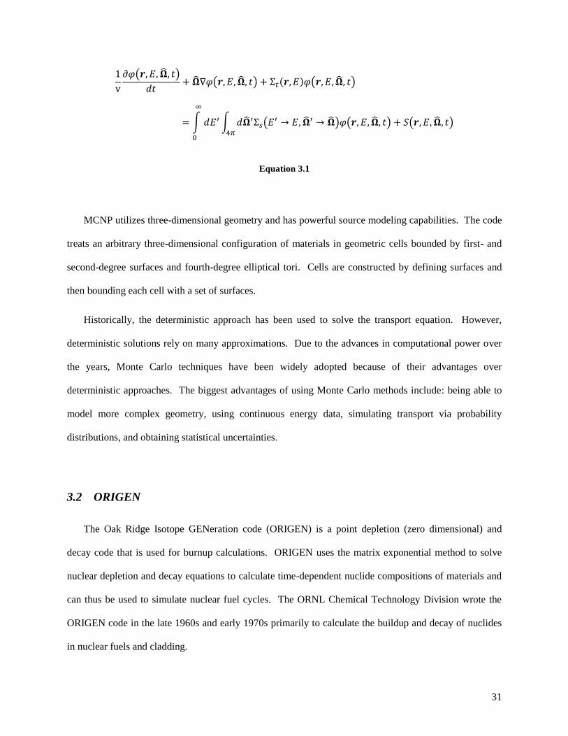
31
Equation 3.1
MCNP utilizes three-dimensional geometry and has powerful source modeling capabilities. The code
treats an arbitrary three-dimensional configuration of materials in geometric cells bounded by first- and
second-degree surfaces and fourth-degree elliptical tori. Cells are constructed by defining surfaces and
then bounding each cell with a set of surfaces.
Historically, the deterministic approach has been used to solve the transport equation. However,
deterministic solutions rely on many approximations. Due to the advances in computational power over
the years, Monte Carlo techniques have been widely adopted because of their advantages over
deterministic approaches. The biggest advantages of using Monte Carlo methods include: being able to
model more complex geometry, using continuous energy data, simulating transport via probability
distributions, and obtaining statistical uncertainties.
3.2 ORIGEN
The Oak Ridge Isotope GENeration code (ORIGEN) is a point depletion (zero dimensional) and
decay code that is used for burnup calculations. ORIGEN uses the matrix exponential method to solve
nuclear depletion and decay equations to calculate time-dependent nuclide compositions of materials and
can thus be used to simulate nuclear fuel cycles. The ORNL Chemical Technology Division wrote the
ORIGEN code in the late 1960s and early 1970s primarily to calculate the buildup and decay of nuclides
in nuclear fuels and cladding.
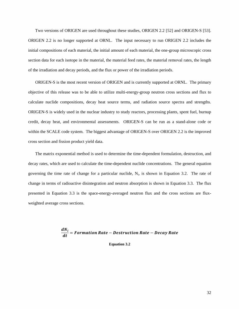
32
Two versions of ORIGEN are used throughout these studies, ORIGEN 2.2 [52] and ORIGEN-S [53].
ORIGEN 2.2 is no longer supported at ORNL. The input necessary to run ORIGEN 2.2 includes the
initial compositions of each material, the initial amount of each material, the one-group microscopic cross
section data for each isotope in the material, the material feed rates, the material removal rates, the length
of the irradiation and decay periods, and the flux or power of the irradiation periods.
ORIGEN-S is the most recent version of ORIGEN and is currently supported at ORNL. The primary
objective of this release was to be able to utilize multi-energy-group neutron cross sections and flux to
calculate nuclide compositions, decay heat source terms, and radiation source spectra and strengths.
ORIGEN-S is widely used in the nuclear industry to study reactors, processing plants, spent fuel, burnup
credit, decay heat, and environmental assessments. ORIGEN-S can be run as a stand-alone code or
within the SCALE code system. The biggest advantage of ORIGEN-S over ORIGEN 2.2 is the improved
cross section and fission product yield data.
The matrix exponential method is used to determine the time-dependent formulation, destruction, and
decay rates, which are used to calculate the time-dependent nuclide concentrations. The general equation
governing the time rate of change for a particular nuclide, Ni, is shown in Equation 3.2. The rate of
change in terms of radioactive disintegration and neutron absorption is shown in Equation 3.3. The flux
presented in Equation 3.3 is the space-energy-averaged neutron flux and the cross sections are flux-
weighted average cross sections.
Equation 3.2

33
Equation 3.3
Where: i = 1, . . ., I
γ is the yield
σf is the microscopic fission cross section
ϕ is the neutron flux
σc is the microscopic capture cross section
λ is the radioactive decay constant
is the yield rate of Ni due to the fission of all nuclides Nj
is the rate of transmutation into Ni due to radioactive neutron capture by Ni-1
is the rate of formation of Ni due to the radioactive decay of Ni’
is the destruction rate of Ni due to fission
is the destruction rate due to all forms of neutron absorption other than fission
is the radioactive decay rate of Ni
Equation 3.3 can be written in matrix notation form (Equation 3.4) since it is composed of a coupled
set of linear first-order differential equations. The N vector in Equation 3.4 is composed of the nuclide
concentrations and the A matrix is the transition matrix that contains the rate coefficients.
34
Equation 3.4
The known solution to Equation 3.4 is shown in Equation 3.5 where the No vector contains the initial
nuclide concentrations. The matrix exponential function shown in Equation 3.6 can be inserted into
Equation 3.5 to form the matrix exponential method. For more detail on the matrix exponential method
see [53].
Equation 3.5
Equation 3.6
3.3 ALEPH
ALEPH [54] is a generic Monte Carlo depletion tool that was developed and is maintained at the
Studiecentrum voor Kernenergie - Centre d'Etude de l'énergie Nucléaire (SCK-CEN): the Belgian
Nuclear Research Center. ALEPH is an interface code between NJOY 99.90, ORIGEN 2.2, and any
version of MCNP or MCNPX. NJOY is used for preparing cross section libraries, ORIGEN 2.2 is used
for depletion calculations, and MCNP is used for transport calculations.
Transport calculations are performed via MCNP and continuous-energy nuclear data in order to
generate a very fine multi-energy-group spectrum. A very fine energy structure of 43000 groups is used
to correctly account for the resonance self-shielding effects, especially those associated with 238
U. This

35
group structure is used to create the effective one-group collapsed cross sections needed for the ORIGEN
2.2 calculations. These cross sections are obtained by weighting available point-wise cross section data
with the MCNP calculated fine-group flux. The point-wise cross section data are consistent with the
cross section data used in the MCNP transport calculation since they are both pre-computed based on the
same ENDF/B data files that are generated by NJOY. This process is known as the multi-group binning
approach.
ORIGEN 2.2 as described in the previous section is a point depletion code that performs evolution
calculations. An input file is created for every zone occupied by a material being depleted. These
materials can be depleted by a constant flux irradiation, a constant power irradiation, or simply by
radioactive decay. After the depletion calculations are completed, ALEPH passes on the new material
compositions to build a new MCNP input file. This process repeats until the last irradiation or decay step
has finished. A user-defined fractional absorption criterion (typically 0.9999) is used to truncate the
number of isotopes calculated by ORIGEN and passed on to the new MCNP input. ALEPH calculates
the total absorption of every nuclide and only those nuclides that contribute to 99.99 % of all absorptions
plus all of the initial user specified nuclides are included in the material composition.
The ALEPH input file consists of the ALEPH code options as well as the MCNP input file. The
major ALEPH inputs outlines the materials to be burned, the libraries and executables to be utilized, the
energy group structure, and the irradiation history. The temperature and/or the density of any of the
materials may be changed and the materials in any cell can be replaced with another user-defined material
at any time step to allow for reloading, simulating heating effects in water, and etc. Also, geometry
changes can be made at any time step through the use of surface transformation cards, and thus, control
rod movement can be simulated during the irradiation period, which is very advantageous since the flux
in a core is dependent on the control rod position.

36
3.4 VESTA
VESTA [55] is a generic Monte Carlo depletion tool that was developed and is maintained at
L'Institut de Radioprotection et de Sûreté Nucléaire (IRSN): the French Institute for Radiological
Protection and Nuclear Safety. VESTA was developed and is maintained by the same code developer
who created the ALEPH code. VESTA and ALEPH are similar in theory and application.
VESTA is a generic evolution interface code that couples NJOY 99.90, ORIGEN 2.2, and either
MCNP or MCNPX to ORIGEN 2.2. The VESTA input file is composed of two parts: the VESTA
specific inputs and the MCNP file. The calculation flow is similar to that of ALEPH such that MCNP
performs a steady state transport calculation to create a very fine multi-group energy structure, which is
used to calculate the spectral- and spatial-averaged, one-group cross sections required by ORIGEN 2.2.
Thus, the multi-group binning approach is also applied to VESTA. ORIGEN 2.2 then performs evolution
calculations for every depletion zone based on the data derived from the MCNP calculation. Then, a new
MCNP input file is constructed with the new material compositions truncated via the user-defined fraction
absorption criterion and any user-defined updates such as material temperatures changes, material
densities changes, or geometry changes. This process repeats until the entire irradiation history has been
modeled.
VESTA uses a predictor only approach by default, and thus, the activation cross section data
calculated at the beginning of a time step is used for the entire step. However, VESTA has the option to
use predictor-corrector or predictor-middlestep algorithms. These algorithms can be used to improve the
results of the depletion calculations for long time steps where spectral changes may occur and impact the
evolution calculation.
VESTA allows for constant power or constant flux irradiations and decay. The constant power
irradiations can be defined as the total power of the system, the values of the power for every burnable
material, the power for a specific burnable material, or the power for a set of burnable materials.

37
Constant flux irradiation steps can be applied by defining the flux values for every burnable material, the
flux value for a specific burnable material, or by normalizing the flux distributions. MCNP is used to
calculate the relative flux distribution and then VESTA uses it to calculate the absolute flux and power
levels and then distributes the power production over the burnable materials.
3.5 SCALE
The Standardized Computer Analyses for Licensing Evaluation (SCALE) [56] modular code system
was developed and is maintained at the Oak Ridge National Laboratory under a joint sponsorship with the
U. S. Nuclear Regulatory Commission and the Department of Energy. The SCALE system consists of
well-established computer codes (also referred to as functional modules) and methods within standard
analysis sequences, which are utilized for reactor physics, criticality safety, radiation shielding, cross
section processing, radiation source term determination, spent fuel characterization, and
sensitivity/uncertainty analyses. An input is constructed for the control module corresponding to the
analytical sequence associated with the type of analysis. The sequences are automated, and thus, the data
needed to execute the functional modules are derived from the control module input and the control
module is used to prepare the inputs for the functional modules and then execute them. The functional
modules can either be coupled via the control modules or can be executed as stand-alone calculations.
Some of the control modules and functional modules in the SCALE 6.0 system, which is the version of
SCALE used in these studies, are described in the following paragraphs.
38
3.5.1 CSAS
Criticality Safety Analysis Sequence (CSAS) is a control module in the SCALE code system that is
used for criticality calculations. The SCALE 6.0 system supports CSAS5 [57] and CSAS6 [58]; both of
which provide automated, problem-dependent cross section processing for effective multiplication factor
calculations for three-dimensional systems. CSAS5 utilizes the KENO V.a functional module and
CSAS6 uses KENO-VI for geometry modeling and transport calculations.
Continuous or multi-group energy calculations can be performed in KENO. If a continuous energy
calculation is performed, then the continuous energy cross sections specified in the input are used. If a
multi-group energy calculation is performed, then KENO uses the problem-dependent processed cross
sections. The CSAS control module employs the BONAMI functional module in the calculation
sequence to provide resonance corrected cross sections in the unresolved resonance range, while the
resonance-corrected cross sections in the resolved resonance range are provided by NITAWL or
WORKER, CENTRM, and PMC.
BONAMI processes cross sections in the unresolved resonance range via the Bondarenko method and
the cross sections in the unresolved range are processed by NITAWL, which uses the Nordheim integral
method, or the WORKER, CENTRM, and PMC combination to collapse point-wise continuous energy
cross sections by means of the problem-dependent point-wise continuous neutron flux.
3.5.2 KENO
Two versions of the KENO three-dimensional Monte Carlo transport code are supported in SCALE
6.0: KENO V.a [59] and KENO-VI [60]. The KENO functional module can be used within the CSAS,
TRITON, and TSUNAMI sequences or can be deployed as a stand-alone code. The primary functions of
KENO are to perform effective multiplication factor calculations and to provide energy- and spatially-
dependent fluxes, absorptions, and fissions; energy-dependent leakage terms; and neutron lifetime,
39
generation time, average energy, and mean-free-path data. KENO uses either continuous energy or multi-
group cross section data to solve the transport equation (Equation 3.1). Both of these versions contain a
Pn scattering model in the cross sections, a procedure for matching lethargy boundaries between albedos
and cross sections to extent the usefulness of the albedo feature and restart capabilities.
The KENO programs offer versatile three-dimensional geometry capabilities. KENO V.a allows for
systems to be modeled from cuboids, rectangular parallelepipeds, cylinders, spheres, hemispheres, and
hemicylinders. The geometry is built by constructing units, which can be used to create arrays or lattices.
Units and arrays can be placed at any desired location within a geometry through the use of the hole
option. The drawback to KENO V.a geometry is that units and arrays cannot intersect any geometry
region and must be ―wholly‖ contained within a region.
All of the features employed in KENO V.a are contained in KENO-VI, but KENO-VI has a more
flexible and powerful geometry packaged referred to as the SCALE Generalized Geometry Package
(SGGP). The SGGP allows for modeling any volume that can be constructed using quadratic equations,
geometry intersections, body rotations, and hexagonal and dodecahedra arrays. Although the KENO-VI
geometry package is more powerful than that used in KENO V.a, the added features result in much longer
run times.
3.5.3 ORIGEN-S
See Chapter 3.2.
3.5.4 TRITON
The TRITON [61] control module performs two-dimensional and three-dimensional depletion
calculations and is therefore primarily utilized for fuel cycle analyses. The TRITON sequence couples
either of the KENO Monte Carlo codes (three-dimensional configuration) or the NEWT discrete ordinates

40
code (two-dimensional configuration) to the ORIGEN-S depletion code. TRITON can be used for
problem-specific cross section processing as well as depletion and decay calculations.
In order to perform depletion calculations, transport calculations are repeated in an iterative sequence
alternating with depletion calculations to update burnup-dependent isotopic cross sections and
inventories. If NEWT is used within TRITON, it is used to calculate the weighted, burnup-dependent,
three-group cross sections and the localized fluxes. COUPLE is used to update the ORIGEN-S libraries
and ORIGEN-S is used to perform multi-region burnup calculations. When invoking the KENO-based
sequence, the stochastic three-dimensional approach is used to calculate fluxes and KMART is used to
prepare the three-group cross sections required by COUPLE and ORIGEN-S, which is again used to
perform multi-material depletion calculations. The predictor-corrector approach is used in TRITON to
update the burnup- and spatially-dependent flux since the flux is dependent on the cross sections that are
changing with burnup.
The cross section processing scheme in TRITON is similar to that employed in CSAS, which is
described in previous paragraphs. BONAMI is always used to process the cross sections in the
unresolved resonance energy range and the cross sections in the resolved resonance range are processed
by the CRAWDAD, WORKER, CENTRM, and PMC sequence; by NITAWL; or by using the
Bondarenko factor applied by BONAMI rather than processing the cross sections in the resolved
resonance range.
3.5.5 NEWT
NEWT (New ESC-based Weighting Transport code) [62] is a two-dimensional discrete-ordinates
solver that provides a solution for multi-group transport calculations. NEWT can be run within the
SCALE sequence or as a stand-alone program. NEWT performs two-dimensional neutron transport
calculations and utilizes the Extended Step Characteristic (ESC) approach for spatial discretization on an
41
arbitrary mesh structure. The primary functions of NEWT are to calculate spatial flux distributions within
nuclear systems and to prepare collapsed cross sections. The cross sections can be used to simply execute
NEWT, can be supplied to ORIGEN-S via the TRITON sequence for depletion calculations, or can be
extracted from the output for use in other applications. NEWT can also be used to calculate effective
multiplication factors, forward and adjoint flux solutions, discontinuity factors, diffusion coefficients,
delayed neutron data, and etc.
Discrete-ordinates is a deterministic approach to solving the transport equation and is better suited for
solving problems where differential quantities such as the energy- and spatially-dependent neutron flux
are desired, in comparison to stochastic (Monte Carlo) techniques as previous described. Discrete-
ordinates approaches are derived from the integrodifferential form of the Boltzmann transport equation in
which a finite-difference grid and a number of discrete directions in space are used to treat the space-,
time-, and energy-dependencies.
A coarse-mesh finite-difference acceleration (CMFD) approach has been added to NEWT to speed up
the source-iteration approach which can be slow to converge. The iteration scheme uses inner iterations
to solve the spatial fluxes in each energy group in order to generate updated source terms, and outer
iterations use the source terms to converge all groups. NEWT uses ESC discretization to calculate
transport between sides within each computation cell. The computational cells are developed in the form
of arbitrary polygons that can accurately represent nonorthogonal systems.
3.6 PARET
The Program for the Analysis of Reactor Transients code (PARET), [63] and [64], is a computer code
that couples the neutronic-hydrodynamic-heat transfer equations for research reactors with plate-type
(flat) and pin-type fuel elements. The code can be used to study both steady state and transient behaviors
and was developed to predict consequences of nondestructive accidents. PARET uses reactor point
42
kinetics so solve the neutronics aspect of the analysis. Multiple heat transfer, laminar flow, and turbulent
flow correlations are provided for the heat transfer and hydrodynamic aspects of the problem. The user
has the capability to select the appropriate correlations based on the operational parameters and the range
of data available for the analysis.
The reactor core can be modeled by a set of nested tubes, flat plates in slab geometry, or with round
fuel rods, and can be constructed with up to 50 channels and 19 axial sections. Each channel may have
different power generation, coolant flow, and hydraulic parameters. One-dimensional heat transfer and
hydrodynamics solutions are solved for and reactor point (zero dimensions) kinetics solutions are solved
for. Since there is no thermal coupling between channels, each channel is effectively independent
regarding heat transfer.
The major code inputs include the physical dimensions of the reactor, fluid flow parameters, initial
system pressure, thermal properties of the fuel and clad, inlet moderator parameters, delayed neutron
information, reactivity coefficients, initial reactor power, local neutron flux ratios, and external reactivity
or core power as a function of time. The major outputs include: the elapsed time, the core power, the total
energy generated, the total reactivity, the moderator temperature and mass velocity, the clad surface
temperature, and the fuel centerline and surface temperatures.
3.7 COMSOL
COMSOL Multiphysics is a software package that uses the finite element method for spatial
discretization to solve physics-based systems of PDEs and/or ODEs. Eigenvalue, steady state, and time-
dependent multiphysics simulations can be performed using the predefined (i.e., built-in)
physics/engineering modules or by specifying a system of user-specific PDEs. In these studies, versions
3.5a [65], 4.1 [66], and 4.2 [67] [68] are utilized to solve user-defined PDEs and ODEs. The COMSOL
model builder is setup with an inverted tree structure to allow the user to view the organization of the
43
model and to expand or collapse the branches containing the pertinent steps. The typical steps taken in
order to solve a finite element-based problem with COMSOL include:
1) drawing or importing the geometry,
2) defining the material properties,
3) defining the applicable physics,
4) defining the applicable boundary conditions,
5) creating the mesh,
6) setting up the solver,
7) performing the calculation, and
8) postprocessing the results.
The geometry can be drawn with the built-in geometry package or can be imported from most of the
major CAD programs (AutoCAD, Pro/ENGINEER, SolidWorks, etc.) via the CAD import module. The
geometry can be sketched in 3-D (with space dimensions x, y, and z), 2-D (x, y), 2-D axisymmetric (r, z),
1-D (x), 1-D axisymmetric (r), or 0-D (no spatial variations). The COMSOL CAD package allows the
user to describe the geometry with primitive shapes and curves, user-defined parametric curves, and
Boolean operations.
COMSOL also has a built-in material browser that contains a list of materials with their respective
properties that can be altered or input as a function of the physics (i.e., temperature, pressure, etc.) if the
user considers it necessary. User-defined material libraries can also be created for materials not contained
within the built-in material library or the properties can simply be added to the material library or defined
as domain-dependent variables. Each domain in the geometry is assigned material properties. In
addition, variables can be defined at the global or local (domain, boundary, point, etc.) levels.
The physics needed to solve the defined problem are selected from the list of predefined physics
applications. The built–in physics modules include, but are not limited to: the AC/DC, MEMS, Structural
Mechanics, Heat Transfer, Computational Fluid Dynamics, Chemical Reaction Engineering, and

44
Mathematics modules. The predefined templates are developed to solve typical physics problems;
however, they can be modified to the user’s needs through equation based modeling capabilities and can
be coupled together with other modules, with user defined PDEs/ODEs, or with external coding through a
MATLAB interface. MATLAB scripts can be integrated with COMSOL via the LiveLink for MATLAB,
which allows the user to preprocess data, manipulate the model, and extract/postprocess the results. The
applicable physics are defined for all domains and the boundary conditions are appropriately defined for
all the boundaries and at points if necessary.
The geometry is discretized by dividing it into mesh elements such that the solution can be
approximated by polynomial functions across the elements. COMSOL has an advanced built-in meshing
capability that allows the user to either create a free mesh based on triangular and/or quadrilateral shapes
or to generate a more highly developed user-defined mesh. Nine predefined mesh element sizes exist
from ―extremely coarse‖ to ―extremely fine.‖ In addition, these meshes can be further refined or can be
defined by specifying the element size parameters (maximum element size, maximum element growth
rate, etc.). Other mesh features such as mapped meshes, boundary layers, swept meshes, moving meshes,
and adaptive mesh refinement algorithms are included in COMSOL. A brief description of how
COMSOL forms the discretization of the PDE can be found in Appendix A.
Study nodes define the study type (stationary, time-dependent, eigenvalue, etc.) and the solver
configuration desired to solve the problem. The solver settings including the equations and dependent
variables to be solved, the solver type, the relative tolerances, the damping methods, and etc. are
contained within the solver configuration. COMSOL has built-in, state-of-the-art solvers including the
MUMPS, PARDISO, and SPOOLES direct solvers. Also, iterative methods including the Conjugate
Gradient, GMRES, FGMRES, and BiCGStab algorithms can be employed along with certain
preconditioners. Batch and cluster computing can also be utilized if necessary. Following the setup and
execution of the solver, postprocessing of the results can be performed in COMSOL or via the LiveLink
for MATLAB.

45
4 Critical Experiment Power Distributions
The purpose of this chapter is to validate a methodology for calculating the power density within the
HFIR core interior using MCNP. The core power distribution is one of the key inputs for thermal
hydraulic and reactor kinetics analyses. This validation study was also performed because MCNP is
currently being used in the LEU conversion studies and this validation will be used to assess the range of
applicability for the LEU studies. Monte Carlo methods are currently being utilized for studies including
fuel operating parameters, enrichment-related safety analyses, and fuel performance in regard to
converting the fuel of the HFIR. The methods have been validated for the prediction of flux values in the
reactor target, reflector, and beam tubes, but this study focuses on the prediction of the power density
profile in the reactor core.
In order to validate MCNP via power density comparisons, a set of experimentally measured results
were utilized. Tables A.1 and A.2 in [69] provides two data sets of relative power densities that were
obtained during the HFIRCE-3 experiments. The core conditions corresponding to each of the two
experiments are different, and therefore, provide two unique scenarios to model. The data in Table A.1
was obtained for clean core conditions in which no boron was present in the moderator and the control
elements were at a symmetrical position of 44.536 cm (17.534 inches) withdrawn with respect to the core
axial midplane. This core configuration simulates beginning-of-life conditions in the HFIR. The set of
data listed in Table A.2 was measured under fully poisoned core conditions in which 1.35 grams of boron
per liter of moderator was present and the control elements were fully withdrawn. This core
configuration simulates end-of-life conditions in the HFIR in which the control and safety elements are
fully withdrawn and the boron in the coolant is used to simulate the poisoning effect of fission products
and loss of reactivity due to fuel consumption during the cycle.
In the past, the BOLD VENTURE diffusion code and the DORT deterministic transport code have
been used to calculate power densities in the reactor core ([27], [70], and [71]), but these models were
simplified representations of the reactor and were two-dimensional (2-D). Also, all of the previous power

46
density calculations have been compared to data interpolated from and fitted to the measured results
reported. This study focuses on using a transport code and a detailed 3-D geometry of the reactor rather
than a simplified 2-D geometry, and calculating power densities to be directly compared to the measured
results rather than to data interpolated and extrapolated from these measured values. The Monte Carlo
method, examined here, coupled with continuous point energy data for neutron cross sections, should
provide the most accurate computational model possible of the critical experiments.
4.1 Background of Critical Experiments
Before HFIR operated at full power, four sets of critical experiments were conducted in order to
finalize the design. This study focuses on the third set of experiments, HFIRCE-3, which produced power
distribution data among numerous other physics parameters. The major differences between the critical
experiment cores include the amount of 235
U in the fuel elements, the amount of 10
B in the inner fuel
element, and the material and region lengths of the components of the control elements. The original
amount of 235
U and 10
B in the HFIRCE-3 core was 9.4 kg and 2.12 g, respectively, but due to control
element upgrades, the amount of 10
B was revised to 2.80 g. A summary of the 235
U and 10
B loadings, as
well as the control elements utilized in the critical experiments is listed in Table 4.1.
Table 4.1. Summary of critical experiments.
Experiment 235
U loading (kg) 10
B Loadinga (g) Control elements
b
CE-2 8.01 1.7 Al, Ni, Ag-Cu
CE-2 8.01 1.7 Al, Ag-Al, Ag-Cu
CE-3 9.40 2.12 Al, Ag-Al, Ag-Cu
CE-3 9.40 3.60 Al, Ag-Al, Ag-Cu
CE-3c 9.40 2.80 Al, Ta-Al, Eu2O3-Al
CE-4 9.40 2.80 Al, Ta-Al, Eu2O3-Al
Today 9.40 2.80 Al, Ta-Al, Eu2O3-Al aOnly in inner fuel element
bIn the form white, grey, and black regions
cBasis of this study
47
In order to obtain the relative power distributions, special fuel elements were fabricated with some
removable fuel plates of the same fuel and poison loading as the fixed plates in the IFE and OFE. ―Foils,‖
chunks of the fuel meat and clad, were punched out of the plates and were reinserted into the plate. The
foils were activated during irradiation and activity was counted to measure the fission densities, which
were converted to and documented as the relative power densities. The locations and dimensions of the
foils are illustrated in Figure 4.1. Three foils are distributed axially along the inner edge, center, and outer
edge in order to obtain a 2-D power distribution. Since the axial midplane is expected to have the highest
power density, six foils were punched at the axial center of the plate in order to better obtain a
representation of the power distribution at the center. Since the plates are symmetric about the vertical
centerline, only half of the plate is shown. The foils that are located below the centerline are suffixed
with the letters E, F, G, HH, and H. The drawing is not to scale and the dimensions are recorded in
centimeters and correspond to the axial height and the arc distance from the involute generating circle.
Up to six plates in each element were used, but due to the symmetry of the core, it was determined
that only three plates in each fuel element were necessary to obtain satisfactory power distribution data
and the circumferential locations 97a in the IFE and 207b in the OFE constituted the best average
removable plate locations. Power distributions were obtained for different control rod positions, poisoned
moderator conditions, and flux trap loadings.
Before the removable plates and foils were inserted into the core and irradiated, the foils were
counted in a scintillation counter, and the weight of 235
U was determined. After irradiation, the foils were
counted in a high pressure, well-type gamma ionization chamber. The relative power densities were
obtained by comparing the total gamma activity of each of the foils with the time interpolated activity of a
normalizing foil that had been irradiated at the same time and was counted periodically during the
counting of the other foils [69].

48
Figure 4.1. Location of foils punched out of removable plates (dimensions in cm).
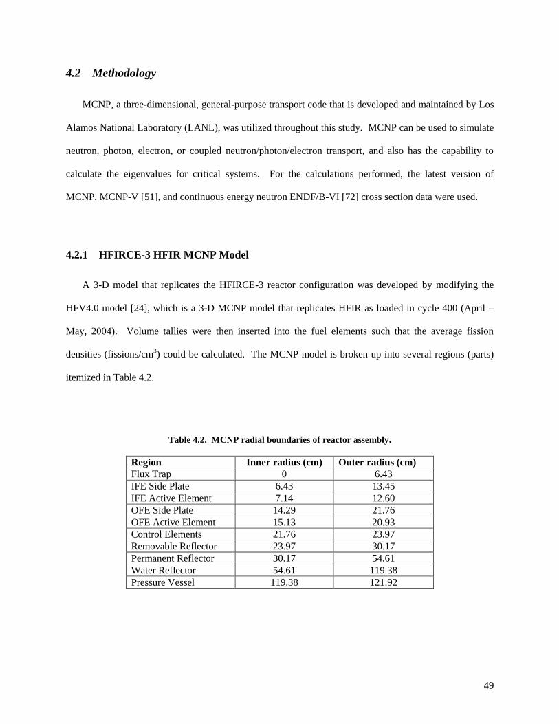
49
4.2 Methodology
MCNP, a three-dimensional, general-purpose transport code that is developed and maintained by Los
Alamos National Laboratory (LANL), was utilized throughout this study. MCNP can be used to simulate
neutron, photon, electron, or coupled neutron/photon/electron transport, and also has the capability to
calculate the eigenvalues for critical systems. For the calculations performed, the latest version of
MCNP, MCNP-V [51], and continuous energy neutron ENDF/B-VI [72] cross section data were used.
4.2.1 HFIRCE-3 HFIR MCNP Model
A 3-D model that replicates the HFIRCE-3 reactor configuration was developed by modifying the
HFV4.0 model [24], which is a 3-D MCNP model that replicates HFIR as loaded in cycle 400 (April –
May, 2004). Volume tallies were then inserted into the fuel elements such that the average fission
densities (fissions/cm3) could be calculated. The MCNP model is broken up into several regions (parts)
itemized in Table 4.2.
Table 4.2. MCNP radial boundaries of reactor assembly.
Region Inner radius (cm) Outer radius (cm)
Flux Trap 0 6.43
IFE Side Plate 6.43 13.45
IFE Active Element 7.14 12.60
OFE Side Plate 14.29 21.76
OFE Active Element 15.13 20.93
Control Elements 21.76 23.97
Removable Reflector 23.97 30.17
Permanent Reflector 30.17 54.61
Water Reflector 54.61 119.38
Pressure Vessel 119.38 121.92

50
The IFE is modeled by dividing it into 56 cells; 8 radial fuel regions and 7 axial fuel layers, and the
OFE is modeled by dividing it into 63 cells; 9 radial fuelled regions and 7 axial fuelled layers. The radial
regions represent the different effective 235
U concentrations (atoms/barn-cm) in the radial direction of the
fuel plate. The fuel is modeled by homogenizing the uranium ―meat,‖ aluminum, and water between the
plates into several radial fuelled regions. Figure 4.2 depicts one of the 171 involute shaped IFE plates.
Table 4.3 lists the inner and outer radii that correspond to the IFE and OFE fuel radial regions.
Figure 4.2. Involute IFE plate.
Aluminum
Cladding

51
Table 4.3. Fuel radial region boundaries.
Fuelled
region
IFE inner
radius (cm)
IFE outer
radius (cm)
OFE inner
radius (cm)
OFE outer
radius (cm)
1 7.14 7.50 15.15 15.50
2 7.50 8.00 15.50 16.00
3 8.00 8.50 16.00 16.50
4 8.50 9.50 16.50 17.50
5 9.50 10.50 17.50 18.50
6 10.50 11.50 18.50 19.50
7 11.50 12.00 19.50 20.00
8 12.00 12.60 20.00 20.50
9 - - 20.50 21.00
The composition of the beryllium in all of the parts of the reflector is the same; however, the presence
of cooling water channels causes homogenized atom densities for the three reflector regions to differ.
The permanent beryllium reflector extends approximately 20 cm beyond the outside radius of the
semipermanent reflector and is surrounded by approximately 50 cm of water. Equilibrium poisons (Li-6
and He-3) resulting from fast neutron reactions in beryllium are modeled in a zone-wise fashion in the
reflector. The main differences (and some similarities) between the cycle 400 production core and the
HFIRCE-3 core are listed in Table 4.4. Differences not listed in Table 4.4 are mostly material (atomic
density) differences.

52
Table 4.4. Summary of cycle 400 production core and HFIRCE-3.
Cycle 400 HFIRCE-3
2.80 g 10
B Loading in IFE 2.80 g 10
B Loading in IFE
9.40 kg 235
U 9.40 kg 235
U
Target Bundle in Flux Trap (Plastic Island + Water) in Flux Trap
Horizontal Beam Tube-2 was Enlarged and Upgraded Horizontal Beam Tube-2 was of Nominal Size
2 Engineering Facilities (Slant Tubes) 4 Engineering Facilities (Slant Tubes)
Horizontal Beam Tube-4 was Enlarged
and Cold Source Inserted
Horizontal Beam Tube-4 was of Nominal Size
8 Large Removable Beryllium Facilities 4 Large Removable Beryllium Facilities
Pressurized Open to Atmosphere
Water Flow to Remove Heat Stagnant Flow
85 MW Essentially Zero Power
At the time of the critical experiments, there were three, nominally 10.16 cm ID horizontal beam
tubes that extended outward from the reactor core at the midplane. HB-4 was originally the location of a
30-m small angle neutron scattering facility and was enlarged and transformed into a high performance
hydrogen cold source in 2007. HB-2, originally the location of a triple-axis spectrometer, was also
enlarged and altered, and now supports a neutron powder diffractometer, a neutron residual stress
mapping facility, and a wide angle neutron diffractometer. During the enlargement of HB-2, two of the
four slant engineering facilities were eliminated. Also, the number of large removable beryllium (RB)
facilities was increased from the original number of four to eight. A cross section of HFIRCE-3 at the
horizontal midplane as modeled with MCNP is illustrated in Figure 4.3.
During the critical experiments, a flux trap target referred to as a plastic island filled with water (PI
+W) flux trap was utilized. The (PI + W) flux trap consisted of a polyethylene insert that was located
within an aluminum tube positioned on top of a stainless steel sinker plate. The polyethylene target
actually had two configurations and was either a solid polyethylene target or a polyethylene cylinder
filled with water. The central (green) area in Figure 4.4 is the water region, the blue region is the
polyethylene insert, the red top and bottom regions represent the aluminum tube lifting plate and the
aluminum end plate, and the light blue area at the bottom of the flux trap is the steel sinker plate.
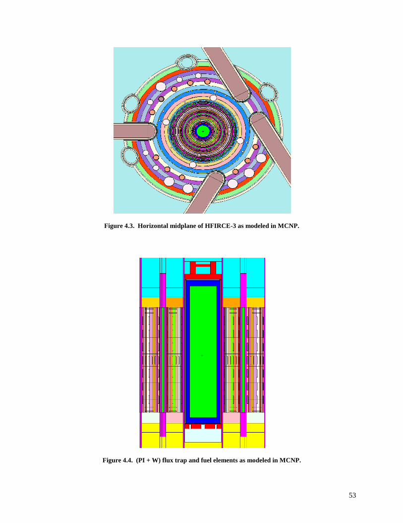
53
Figure 4.3. Horizontal midplane of HFIRCE-3 as modeled in MCNP.
Figure 4.4. (PI + W) flux trap and fuel elements as modeled in MCNP.
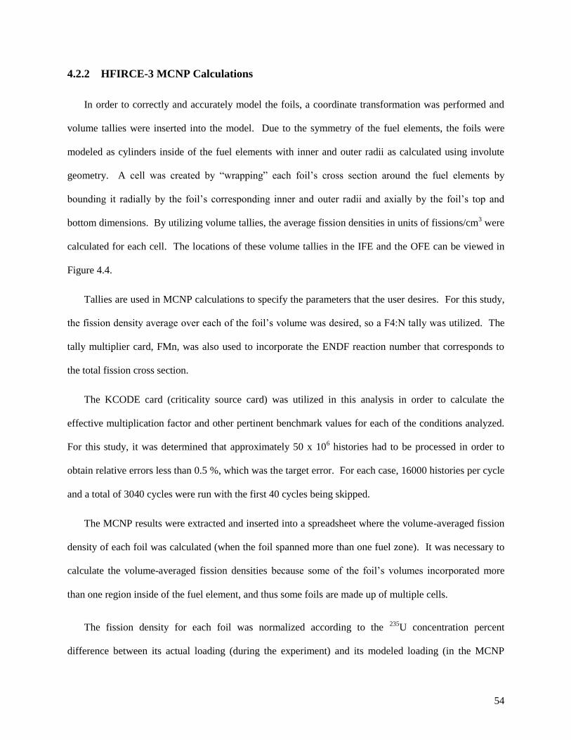
54
4.2.2 HFIRCE-3 MCNP Calculations
In order to correctly and accurately model the foils, a coordinate transformation was performed and
volume tallies were inserted into the model. Due to the symmetry of the fuel elements, the foils were
modeled as cylinders inside of the fuel elements with inner and outer radii as calculated using involute
geometry. A cell was created by ―wrapping‖ each foil’s cross section around the fuel elements by
bounding it radially by the foil’s corresponding inner and outer radii and axially by the foil’s top and
bottom dimensions. By utilizing volume tallies, the average fission densities in units of fissions/cm3 were
calculated for each cell. The locations of these volume tallies in the IFE and the OFE can be viewed in
Figure 4.4.
Tallies are used in MCNP calculations to specify the parameters that the user desires. For this study,
the fission density average over each of the foil’s volume was desired, so a F4:N tally was utilized. The
tally multiplier card, FMn, was also used to incorporate the ENDF reaction number that corresponds to
the total fission cross section.
The KCODE card (criticality source card) was utilized in this analysis in order to calculate the
effective multiplication factor and other pertinent benchmark values for each of the conditions analyzed.
For this study, it was determined that approximately 50 x 106 histories had to be processed in order to
obtain relative errors less than 0.5 %, which was the target error. For each case, 16000 histories per cycle
and a total of 3040 cycles were run with the first 40 cycles being skipped.
The MCNP results were extracted and inserted into a spreadsheet where the volume-averaged fission
density of each foil was calculated (when the foil spanned more than one fuel zone). It was necessary to
calculate the volume-averaged fission densities because some of the foil’s volumes incorporated more
than one region inside of the fuel element, and thus some foils are made up of multiple cells.
The fission density for each foil was normalized according to the 235
U concentration percent
difference between its actual loading (during the experiment) and its modeled loading (in the MCNP
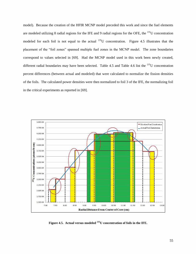
55
model). Because the creation of the HFIR MCNP model preceded this work and since the fuel elements
are modeled utilizing 8 radial regions for the IFE and 9 radial regions for the OFE, the 235
U concentration
modeled for each foil is not equal to the actual 235
U concentration. Figure 4.5 illustrates that the
placement of the ―foil zones‖ spanned multiple fuel zones in the MCNP model. The zone boundaries
correspond to values selected in [69]. Had the MCNP model used in this work been newly created,
different radial boundaries may have been selected. Table 4.5 and Table 4.6 list the 235
U concentration
percent differences (between actual and modeled) that were calculated to normalize the fission densities
of the foils. The calculated power densities were then normalized to foil 3 of the IFE, the normalizing foil
in the critical experiments as reported in [69].
Figure 4.5. Actual versus modeled 235
U concentration of foils in the IFE.

56
Table 4.5. Percent difference of 235
U modeled in IFE.
Foil Actual
(atoms/b-cm)
Modeled
(atoms/b-cm)
Act. – Mod.
(atoms/b-cm)
Percent
difference
1 2.13403E-04 2.10202E-04 3.20094E-06 1.49995
2 3.18892E-04 3.11260E-04 7.63201E-06 2.39329
3 4.12780E-04 3.86333E-04 2.64478E-05 6.40723
4 4.62314E-04 4.49159E-04 1.31547E-05 2.84539
5 4.36756E-04 4.45758E-04 -9.00188E-06 -2.06108
6 3.57157E-04 3.71800E-04 -1.46435E-05 -4.10001
A, AA, HH, H 4.42420E-04 4.38301E-04 4.12233E-06 0.93176
Table 4.6. Percent difference of 235
U modeled in OFE.
Foil Actual
(atoms/b-cm)
Modeled
(atoms/b-cm)
Act. – Mod.
(atoms/b-cm)
Percent
difference
1 4.46150E-04 4.33139E-04 1.30114E-05 2.91637
2 6.36438E-04 6.25508E-04 1.09304E-05 1.71743
3 6.83048E-04 6.57861E-04 2.51869E-05 3.68742
4 5.73625E-04 5.29200E-04 4.44254E-05 7.74468
5 4.22050E-04 4.14500E-04 7.55016E-06 1.78892
6 2.60472E-04 2.69800E-04 -9.32814E-06 -3.58125
A, AA, HH, H 5.68618E-04 5.66674E-04 1.94412E-06 0.34190

57
4.3 HFIRCE-3 Results
Two conditions were analyzed during this study: a clean core condition and a fully poisoned
condition. The clean core condition consisted of no boron in the moderator and the control elements at
symmetric positions of 44.536 cm (17.534 in) withdrawn with respect to the axial midplane. This
experiment was performed on September 9, 1965. For the fully poisoned condition, the control elements
were fully withdrawn and 1.35 grams of boron per liter in the moderator was used to control reactivity.
This experiment was performed on October 5, 1965.
It is important to note that the power densities have been normalized to foil 3 of the IFE, not to the
average core power density. The average power density of foil 3 is approximately 25 % greater than the
average core power density. It is also important to note that the experimental relative power densities
being compared in this analysis correspond to plate positions 97a and 207b for the IFE and OFE,
respectively, and the uncertainties reported represent 3 standard deviations.
4.3.1 Clean Core Results
The calculated eigenvalue (keff) under the clean core conditions was 0.99561 ± 0.00013, so the model
does accurately predict the multiplication factor for the reactor to within 1 %. The results for the final
MCNP criticality calculations for the clean core conditions are listed in Table 4.7.
Table 4.7. Effective multiplication factors for clean core conditions.
keff estimator keff Standard
deviation
68 %
confidence
95 %
confidence
99 %
confidence
Collision 0.99546 0.00019 0.99527 to 0.99565 0.99508 to 0.99584 0.99496 to 0.99596
Absorption 0.99565 0.00013 0.99551 to 0.99578 0.99538 to 0.99592 0.99529 to 0.99601
Track length 0.99543 0.00020 0.99523 to 0.99562 0.99503 to 0.99582 0.99490 to 0.99595
col/abs/trk len 0.99561 0.00013 0.99548 to 0.99574 0.99535 to 0.99587 0.99526 to 0.99596

58
Some of the pertinent calculated values are listed below:
the final combined (col/abs/tl) prompt removal lifetime = 1.4676 x 10-04
± 9.5564 x 10-08
seconds,
the average neutron energy causing fission = 2.3371 x 10-02
MeV,
the energy corresponding to the average neutron lethargy causing fission = 1.6438 x 10-07
MeV,
the percentages of fissions caused by neutrons in the thermal, intermediate, and fast neutron
ranges are: (<0.625 eV): 83.26 % (0.625 eV – 100 keV): 15.26 % (>100 keV): 1.48 %,
the average fission neutrons produced per neutron absorbed (capture + fission) in all cells with
fission = 1.7361,
the average fission neutrons produced per neutron absorbed (capture + fission) in all the geometry
cells = 9.7752 x 10-01
, and
the average number of neutrons produced per fission = 2.438.
The radial relative power profile at the horizontal midplane is shown in Figure 4.6, which is
composed of data derived from foils 1 through 6 for both the inner and outer fuel elements. The axial
relative power profiles corresponding to foils 1B-1G, 4A-4H, and 6B-6G for both the inner and outer fuel
elements are shown in Figure 4.7 through Figure 4.12, respectively. Reflector savings can be observed in
Figure 4.6, Figure 4.8, and Figure 4.11 because foils located at the edges are analyzed in these figures and
water is located at these edges.
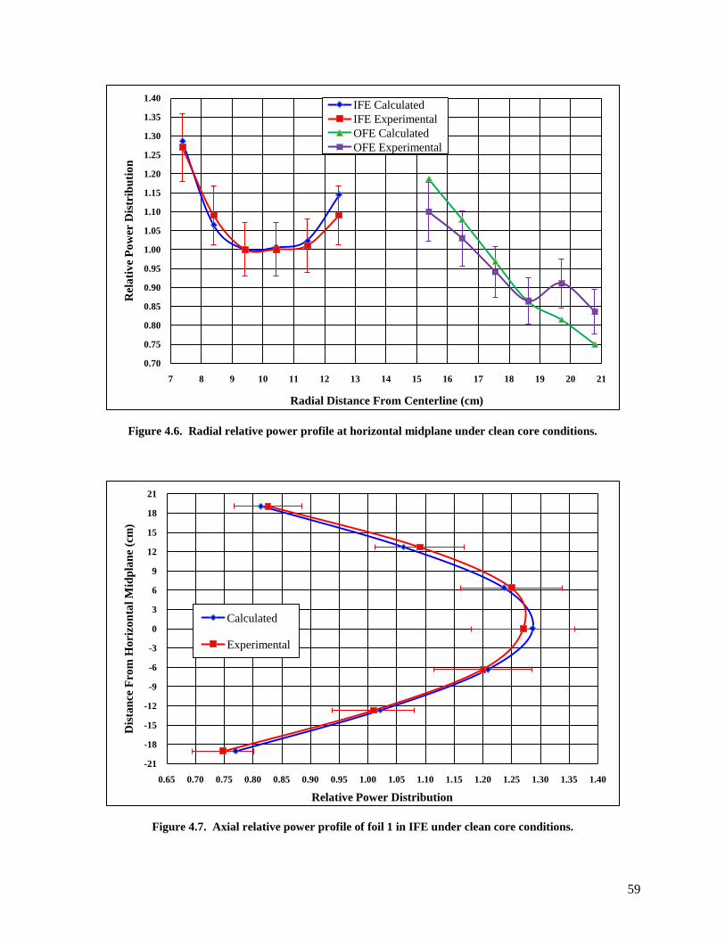
59
Figure 4.6. Radial relative power profile at horizontal midplane under clean core conditions.
Figure 4.7. Axial relative power profile of foil 1 in IFE under clean core conditions.
0.70
0.75
0.80
0.85
0.90
0.95
1.00
1.05
1.10
1.15
1.20
1.25
1.30
1.35
1.40
7 8 9 10 11 12 13 14 15 16 17 18 19 20 21
Rel
ati
ve
Po
wer
Dis
trib
uti
on
Radial Distance From Centerline (cm)
IFE Calculated
IFE Experimental
OFE Calculated
OFE Experimental
-21
-18
-15
-12
-9
-6
-3
0
3
6
9
12
15
18
21
0.65 0.70 0.75 0.80 0.85 0.90 0.95 1.00 1.05 1.10 1.15 1.20 1.25 1.30 1.35 1.40
Dis
tan
ce F
rom
Ho
rizo
nta
l M
idp
lan
e (c
m)
Relative Power Distribution
Calculated
Experimental

60
Figure 4.8. Axial relative power profile of foil 4 in IFE under clean core conditions.
Figure 4.9. Axial relative power profile of foil 6 in IFE under clean core conditions.
-27
-24
-21
-18
-15
-12
-9
-6
-3
0
3
6
9
12
15
18
21
24
27
0.45 0.50 0.55 0.60 0.65 0.70 0.75 0.80 0.85 0.90 0.95 1.00 1.05 1.10
Dis
tan
ce F
rom
Ho
rizo
nta
l M
idp
lan
e (c
m)
Relative Power Distribution
Calculated
Experimental
-21
-18
-15
-12
-9
-6
-3
0
3
6
9
12
15
18
21
0.60 0.65 0.70 0.75 0.80 0.85 0.90 0.95 1.00 1.05 1.10 1.15 1.20
Dis
tan
ce F
rom
Ho
rizo
nta
l M
idp
lan
e (c
m)
Relative Power Distribution
Calculated
Experimental

61
Figure 4.10. Axial relative power profile of foil 1 in OFE under clean core conditions.
Figure 4.11. Axial relative power profile of foil 4 in OFE under clean core conditions.
-21
-18
-15
-12
-9
-6
-3
0
3
6
9
12
15
18
21
0.55 0.60 0.65 0.70 0.75 0.80 0.85 0.90 0.95 1.00 1.05 1.10 1.15 1.20 1.25
Dis
tan
ce F
rom
Ho
rizo
nta
l M
idp
lan
e (c
m)
Relative Power Distribution
Calculated
Experimental
-27
-24
-21
-18
-15
-12
-9
-6
-3
0
3
6
9
12
15
18
21
24
27
0.25 0.30 0.35 0.40 0.45 0.50 0.55 0.60 0.65 0.70 0.75 0.80 0.85 0.90 0.95
Dis
tan
ce F
rom
Ho
rizo
nta
l M
idp
lan
e (c
m)
Relative Power Distribution
Calculated
Experimental
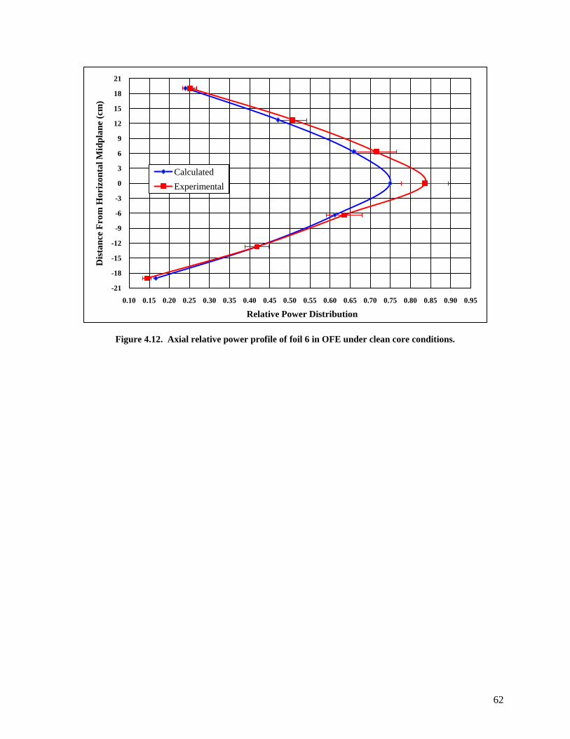
62
Figure 4.12. Axial relative power profile of foil 6 in OFE under clean core conditions.
-21
-18
-15
-12
-9
-6
-3
0
3
6
9
12
15
18
21
0.10 0.15 0.20 0.25 0.30 0.35 0.40 0.45 0.50 0.55 0.60 0.65 0.70 0.75 0.80 0.85 0.90 0.95
Dis
tan
ce F
rom
Ho
rizo
nta
l M
idp
lan
e (c
m)
Relative Power Distribution
Calculated
Experimental

63
4.3.2 Fully Poisoned Results
The calculated eigenvalue (keff) under the fully poisoned conditions was 1.00593 ± 0.00013, so the
model does accurately predict the multiplication factor for the reactor to within 1 %. The results for the
final MCNP criticality calculations for the fully poisoned core condition are listed in Table 4.8. Some of
the pertinent calculated values are listed below:
the final combined (col/abs/tl) prompt removal lifetime = 1.9343 x 10-04
± 1.2738 x 10-07
seconds,
the average neutron energy causing fission = 2.2789 x 10-02
MeV,
the energy corresponding to the average neutron lethargy causing fission = 1.6314 x 10-07
MeV,
the percentages of fissions caused by neutrons in the thermal, intermediate, and fast neutron
ranges are: (<0.625 eV): 83.37 % (0.625 eV – 100 keV): 15.20 % (>100 keV): 1.44 %,
the average fission neutrons produced per neutron absorbed (capture + fission) in all cells with
fission = 1.6195,
the average fission neutrons produced per neutron absorbed (capture + fission) in all the geometry
cells = 9.8580 x 10-01
, and
the average number of neutrons produced per fission = 2.439.
Table 4.8. Effective multiplication factors for poisoned core conditions.
keff estimator keff Standard
deviation
68 %
confidence
95 %
confidence
99 %
confidence
collision 1.00595 0.00018 1.00577 to 1.00613 1.00559 to 1.00630 1.00548 to 1.00642
absorption 1.00593 0.00013 1.00580 to 1.00606 1.00567 to 1.00619 1.00558 to 1.00628
track length 1.00593 0.00019 1.00574 to 1.00612 1.00556 to 1.00631 1.00544 to 1.00643
col/abs/trk len 1.00593 0.00013 1.00581 to 1.00606 1.00568 to 1.00618 1.00560 to 1.00626

64
Figure 4.13 shows the radial relative power profile at the horizontal midplane, and is composed of
data derived from foils 1 through 6 for both the inner and outer fuel elements. The axial relative power
profiles corresponding to foils 1B-1G, 4A-4H, and 6B-6G for both the inner and outer fuel elements are
shown in Figure 4.14 through Figure 4.19, respectively. Reflector savings can be observed in Figure
4.13, Figure 4.15, and Figure 4.18 because foils located at the edges are analyzed here and water is
located at these edges.
Figure 4.13. Radial relative power profile at horizontal midplane under fully poisoned core conditions.
0.70
0.75
0.80
0.85
0.90
0.95
1.00
1.05
1.10
1.15
1.20
1.25
1.30
1.35
1.40
1.45
7 8 9 10 11 12 13 14 15 16 17 18 19 20 21
Rel
ati
ve
Po
wer
Dis
trib
uti
on
Radial Distance From Centerline (cm)
IFE Calculated
IFE Experimental
OFE Calculated
OFE Experimental
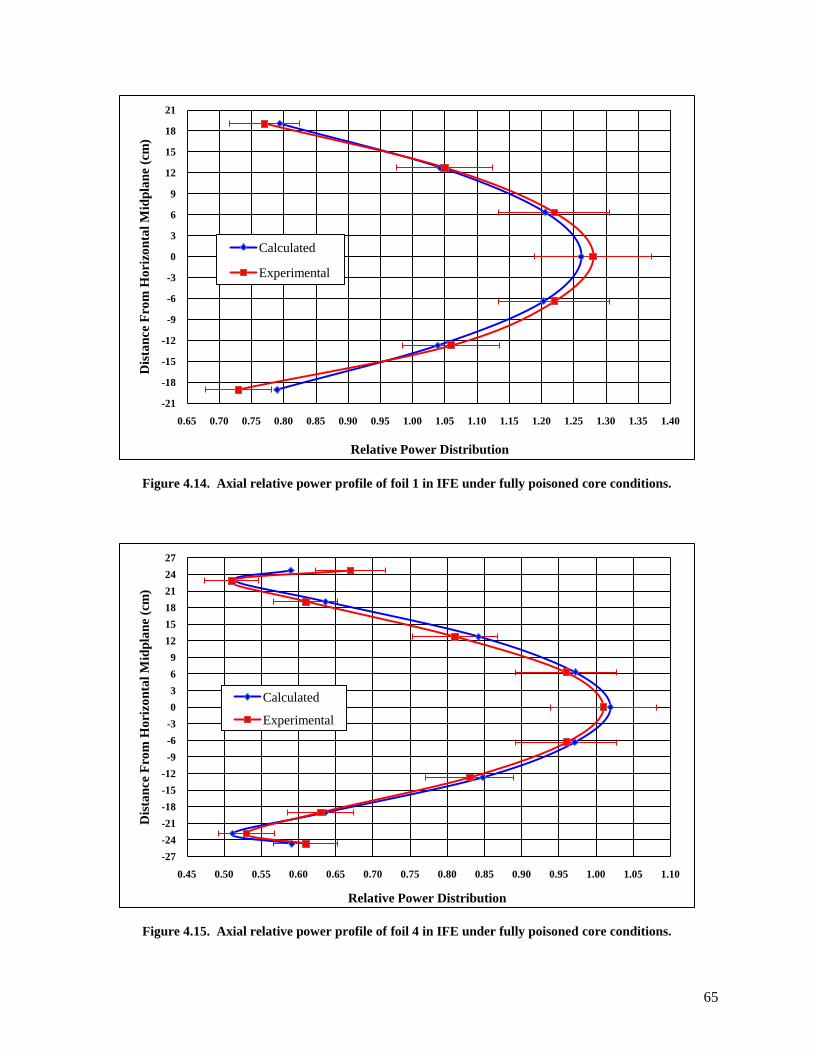
65
Figure 4.14. Axial relative power profile of foil 1 in IFE under fully poisoned core conditions.
Figure 4.15. Axial relative power profile of foil 4 in IFE under fully poisoned core conditions.
-21
-18
-15
-12
-9
-6
-3
0
3
6
9
12
15
18
21
0.65 0.70 0.75 0.80 0.85 0.90 0.95 1.00 1.05 1.10 1.15 1.20 1.25 1.30 1.35 1.40
Dis
tan
ce F
rom
Ho
rizo
nta
l M
idp
lan
e (c
m)
Relative Power Distribution
Calculated
Experimental
-27
-24
-21
-18
-15
-12
-9
-6
-3
0
3
6
9
12
15
18
21
24
27
0.45 0.50 0.55 0.60 0.65 0.70 0.75 0.80 0.85 0.90 0.95 1.00 1.05 1.10
Dis
tan
ce F
rom
Ho
rizo
nta
l M
idp
lan
e (c
m)
Relative Power Distribution
Calculated
Experimental
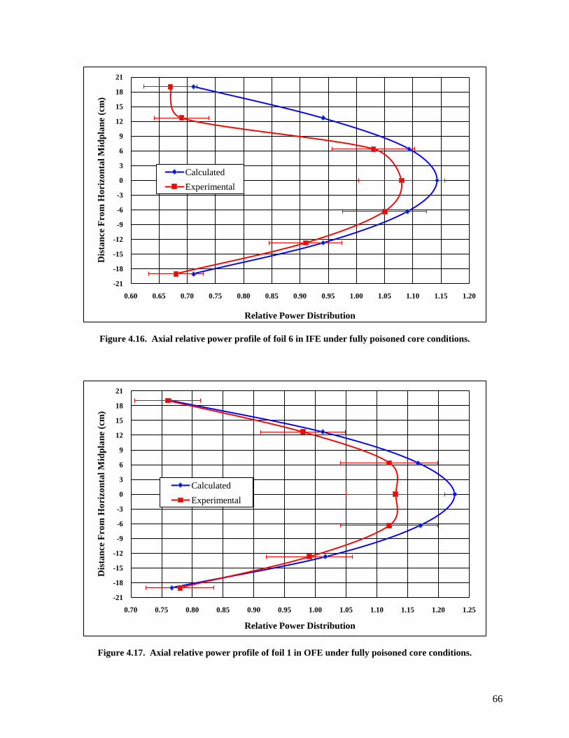
66
Figure 4.16. Axial relative power profile of foil 6 in IFE under fully poisoned core conditions.
Figure 4.17. Axial relative power profile of foil 1 in OFE under fully poisoned core conditions.
-21
-18
-15
-12
-9
-6
-3
0
3
6
9
12
15
18
21
0.60 0.65 0.70 0.75 0.80 0.85 0.90 0.95 1.00 1.05 1.10 1.15 1.20
Dis
tan
ce F
ro
m H
oriz
on
tal
Mid
pla
ne (
cm
)
Relative Power Distribution
Calculated
Experimental
-21
-18
-15
-12
-9
-6
-3
0
3
6
9
12
15
18
21
0.70 0.75 0.80 0.85 0.90 0.95 1.00 1.05 1.10 1.15 1.20 1.25
Dis
tan
ce F
ro
m H
oriz
on
tal
Mid
pla
ne (
cm
)
Relative Power Distribution
Calculated
Experimental
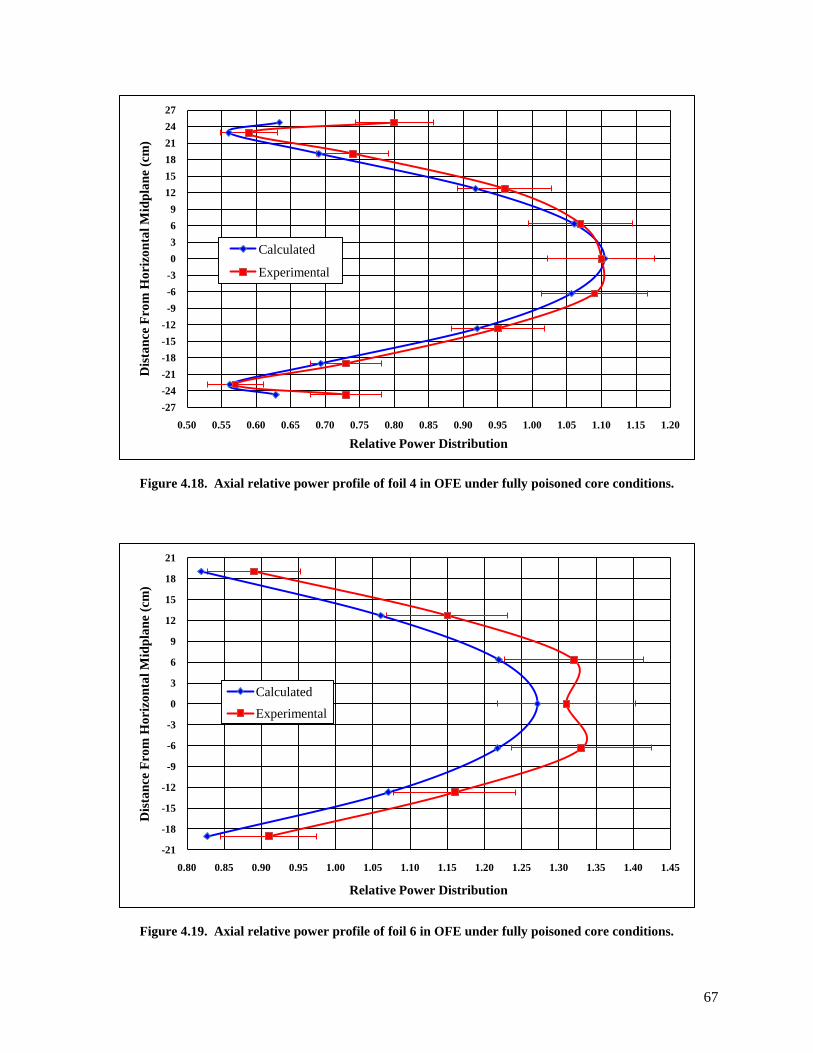
67
Figure 4.18. Axial relative power profile of foil 4 in OFE under fully poisoned core conditions.
Figure 4.19. Axial relative power profile of foil 6 in OFE under fully poisoned core conditions.
-27
-24
-21
-18
-15
-12
-9
-6
-3
0
3
6
9
12
15
18
21
24
27
0.50 0.55 0.60 0.65 0.70 0.75 0.80 0.85 0.90 0.95 1.00 1.05 1.10 1.15 1.20
Dis
tan
ce F
rom
Ho
rizo
nta
l M
idp
lan
e (c
m)
Relative Power Distribution
Calculated
Experimental
-21
-18
-15
-12
-9
-6
-3
0
3
6
9
12
15
18
21
0.80 0.85 0.90 0.95 1.00 1.05 1.10 1.15 1.20 1.25 1.30 1.35 1.40 1.45
Dis
tan
ce F
rom
Ho
rizo
nta
l M
idp
lan
e (c
m)
Relative Power Distribution
Calculated
Experimental

68
4.4 HFIRCE-3 Summary
Critical experiments for HFIR were modeled for two configurations: clean core and fully poisoned
core (designated as configurations from the series HFIRCE-3). Multiplication factors and power density
distributions were calculated and good agreement between the calculated and experimental measurements
was found. Power density profiles revealed that MCNP can calculate power densities with reasonable
confidence within the core interior.
The calculated multiplication factor under the clean core and fully poisoned conditions was 0.99561 ±
0.00013 and 1.00593 ± 0.00013, respectively. The model accurately predicted the multiplication factor
for the reactor to within 1 %. The less than 1 % estimation of keff could be due to many reasons. The
most obvious are the spatially dependent atom densities and nuclear data utilized. A few assumptions
were made in the modeling, and many regions were homogenized. The exact atom density of many
materials and the presence of trace elements effects neutrons, and thus, keff. Also, cross section data are
not perfect, and the results of eigenvalue calculations will vary depending on which library is used.
However, per [69], criticality was not always achieved during the critical experiments, which
rationalizes the subcritical clean core calculation. Also according to [69], acid rinses were performed
periodically and the control elements were ―essentially‖ fully withdrawn for the fully poisoned
experiment. Each of these conditions would introduce negative reactivity that was not explicitly modeled
and justify the 0.00593 overestimation in keff for the poisoned core condition. Per [73], eigenvalues for
critical systems are typically calculated within ± 1 % accuracy for systems utilizing HEU fuel, which was
observed during the validation of KENO-VI, another Monte Carlo code. The 0.00439 underestimation
and the 0.00593 overestimation in keff has essentially no impact on the relative power distributions. After
reviewing the results from this analysis, it was determined that a bias factor is not necessary for current
design studies.
69
5 Exposure-Dependent Nuclide Inventory
The purpose of this chapter is to validate a Monte Carlo-based depletion methodology by comparing
calculated post-irradiation uranium isotopic compositions in the fuel elements of the High Flux Isotope
Reactor core to values measured using uranium mass spectrographic analysis. The spatial power
distribution in HFIR changes significantly as irradiation time increases due to control element movement.
Accurate calculation of the end-of-life uranium isotopic inventory is a good indicator that the power
distribution variation as a function of space and time is accurately calculated, i.e., an integral check.
Time-dependent power distribution profiles are needed for reactor core thermal hydraulic and reactor
kinetics analyses, and thus, the purpose of this chapter is to validate a methodology to accurately calculate
the power distribution for highly enriched uranium (HEU) fuel.
5.1 Post-Irradiation Data
Three sets of post-irradiation uranium isotopic experimental data were obtained from [74]. The report
describes the results of the post-irradiation examination and evaluation of several spent fuel elements
from the High Flux Isotope Reactor (HFIR) that were irradiated in the mid to late 1960s. These fuel
elements were examined in order to determine their overall condition, as well as to ensure no unexpected
problems existed that would compromise continued operations. Gamma scanning and analytical burnup
determinations showed that the time-integrated power and burnup distributions within these fuel elements
agreed well with design predictions. The purpose of this study is to validate a Monte Carlo-based
depletion methodology for calculating the burnup dependent nuclide inventory, specifically the post-
irradiation uranium isotopic composition, for the HFIR core.
A fuel plate from three different fuel elements was selected for post-irradiation burnup examination.
A fuel plate from each element was sectioned for analytical burnup determinations via a water-cooled
abrasive cutoff wheel. Five axial zones were selected for analysis: two nominally minimum burnup
70
regions (top and bottom of the fuel plate), two nominally intermediate burnup regions (between the
horizontal midplane and top and bottom of the fuel plate), and the nominally maximum burnup region
(middle of the fuel plate). These specimens were cut out from the inner (labeled I), outer (labeled O), and
central (labeled H) regions prior to analysis. The samples were then submitted for uranium mass-
spectrographic analysis and the atomic percent of the uranium isotopes was calculated for each sample.
Thus, for each fuel plate examined, 15 specimens were submitted to mass spectrographic analysis. The
locations of the specimens extracted for mass-spectrographic analysis are shown in Figure 5.1.
Fuel elements 5-I (I denotes IFE) and 5-O (O denotes OFE) were present in the first core to operate
continuously at full power in HFIR (cycle 4). This core was brought to power on September 9, 1966 and
operated at 100 MW until September 30th when a plant-wide electrical failure caused a premature
shutdown after 2046 MWd of operation. The in-reactor performance was slightly affected by a special
pretreatment given to fuel elements in the first few HFIR fuel cores. Fuel element 5 was immersed in
boiling deionized water for 24 hours before being placed in the reactor. This was done to increase
corrosion resistance during pre-operation and low-power runs. The corrosion-product films on the
surfaces of the fuel plates were thicker than the other elements. Pretreatment was performed because fuel
elements were often placed in the reactor pool for up to three months before being placed in the reactor.
The pretreatment was used to produce a thin semi-protective oxide film on the fuel plate surfaces to avoid
the formation of a thick, gelatinous, corrosion product film prior to being placed into service. Following
irradiation, these elements were stored in the fuel pool until October 12, 1967, when they were transferred
to the High Radiation Level Examination Laboratory (HRLEL) hot cells for examination.

71
Figure 5.1. Axial and radial locations of burnup specimens (cm).
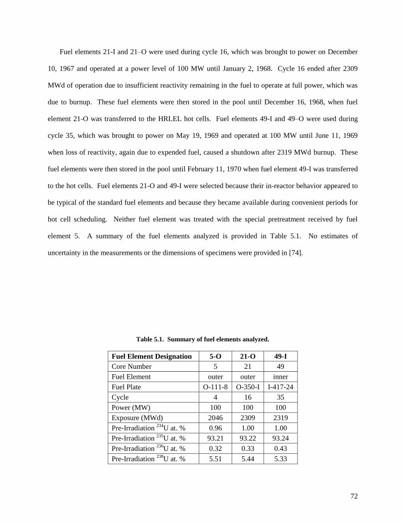
72
Fuel elements 21-I and 21–O were used during cycle 16, which was brought to power on December
10, 1967 and operated at a power level of 100 MW until January 2, 1968. Cycle 16 ended after 2309
MWd of operation due to insufficient reactivity remaining in the fuel to operate at full power, which was
due to burnup. These fuel elements were then stored in the pool until December 16, 1968, when fuel
element 21-O was transferred to the HRLEL hot cells. Fuel elements 49-I and 49–O were used during
cycle 35, which was brought to power on May 19, 1969 and operated at 100 MW until June 11, 1969
when loss of reactivity, again due to expended fuel, caused a shutdown after 2319 MWd burnup. These
fuel elements were then stored in the pool until February 11, 1970 when fuel element 49-I was transferred
to the hot cells. Fuel elements 21-O and 49-I were selected because their in-reactor behavior appeared to
be typical of the standard fuel elements and because they became available during convenient periods for
hot cell scheduling. Neither fuel element was treated with the special pretreatment received by fuel
element 5. A summary of the fuel elements analyzed is provided in Table 5.1. No estimates of
uncertainty in the measurements or the dimensions of specimens were provided in [74].
Table 5.1. Summary of fuel elements analyzed.
Fuel Element Designation 5-O 21-O 49-I
Core Number 5 21 49
Fuel Element outer outer inner
Fuel Plate O-111-8 O-350-I I-417-24
Cycle 4 16 35
Power (MW) 100 100 100
Exposure (MWd) 2046 2309 2319
Pre-Irradiation 234
U at. % 0.96 1.00 1.00
Pre-Irradiation 235
U at. % 93.21 93.22 93.24
Pre-Irradiation 236
U at. % 0.32 0.33 0.43
Pre-Irradiation 238
U at. % 5.51 5.44 5.33

73
5.2 Computational Model Development
ALEPH [54], a Monte Carlo-based depletion code developed at SCK•CEN in Belgium that links
MCNP and ORIGEN 2.2, and VESTA [55], a Monte Carlo-based depletion code developed at IRSN in
France that links MCNP and ORIGEN 2.2, were utilized for this study. The input files for both codes
consist of the depletion code options as well as the MCNP input file. The major input options for ALEPH
and VESTA include: the materials to be burned, the libraries and executables to be utilized, the group
structure, and the irradiation history. The process coded into both VESTA and ALEPH is similar in that
after processing the input, an MCNP input file is created and executed. Then, ORIGEN libraries and
input files are created based on the neutron spectra for the applicable burnup zones and ORIGEN is then
executed. The process repeats starting with the creation of a new MCNP input file that is updated based
on the new isotopic compositions and any changes listed in the ALEPH/VESTA input options (i.e.,
temperature, density, material, or surface transformation changes).
A Monte Carlo-based methodology was chosen for this study because Monte Carlo simulations are
accurate and powerful for reactor core calculations and allow for complex three-dimensional geometries
to be modeled. Most Monte Carlo burnup codes are demanding on calculation time, but ALEPH and
VESTA speed up the calculation time through the use of the multi-group binning approach. A fine multi-
group spectrum is calculated in MCNP which is used to determine the reaction rates outside of MCNP
and to calculate the one-group collapsed cross sections needed for the ORIGEN calculations. The ability
to accurately model HFIR’s geometry and calculate essential physics parameters in MCNP along with the
proven efficiency of ALEPH and VESTA and the ability to explicitly simulate control element movement
during the cycle are the incentives behind using ALEPH and VESTA in this study.
For this study, version 5 of the MCNP code [51] was employed. Continuous energy neutron
ENDF/B-VI.8 [72] and JENDL 3.3 [75] cross section data were used for the ALEPH calculations and
continuous energy neutron ENDF/B-VII cross section data were used for the VESTA calculations. For
the ALEPH calculation, ENDF/B-VI.8 cross section libraries were used for all nuclides except for those

74
of magnesium and titanium because ENDF/B-VI.8 data are not available for these elements. JENDL 3.3
cross section data were utilized for the isotopes of these two elements. The more recent ENDF/B-VII
library was used with VESTA because calculations were first performed with ALEPH. About a year
later, both VESTA and the ENDF/B-VII library were released, utilized, and compared to the ALEPH
calculations.
The depletion code ORIGEN 2.2 requires one-group collapsed cross sections for the (n,γ), (n,2n),
(n,3n), (n,α), (n,p), and fission reactions. These cross sections are obtained by weighting available point-
wise cross section data with the MCNP calculated fine-group flux. The point-wise cross section data are
consistent with the cross section data used in the MCNP transport calculation since they are both pre-
computed based on the same ENDF/B data files that are generated by NJOY. A total of 43000 energy
groups between 10-5
eV to 20 MeV are used to tally the fine multi-group flux.
All cross section data were used at a temperature of 300 K, which is slightly less than the average
core temperature of approximately 360 K [28]. The typical temperature range in the fuel is approximately
between 340 and 380 K. Reactivity effects such as Doppler effects caused by the difference between the
spatially dependent actual core temperatures and the modeled temperature of 300 K are not significant
[76]. Analyses such as assigning a fraction of the HEU fuel to 300 K and the remainder to 600 K have
been performed on HFIR models and no notable differences were observed.
In order to calculate the post-irradiation uranium isotopic compositions in the fuel elements, an
existing ALEPH/MCNP model [77] that was created for the HFIR fuel cycle designated as cycle 400 was
modified to reflect the cores of cycles 4, 16, and 35. Cells were created in the fuel elements to represent
the locations of the burnup specimens and transformation cards were used to simulate the control element
withdrawal as a function of cycle time. The cores were irradiated at a constant power of 100 MW and the
end-of-life uranium isotopic concentrations were extracted from the outputs and analyzed.

75
5.2.1 HFIR MCNP Model Development
The ALEPH/MCNP model modified for this study is based on the HFIR cycle 400 MCNP model,
which is a 3-D MCNP model, named HFV4.0 [24] that accurately represents the HFIR as loaded in cycle
400 (April – May, 2004). HFV4.0 is based on an older model previously developed at ORNL. These
models are quality-controlled and have been set up such that the user can modify the input cards to reflect
any changes to the model or future experimental rearrangements such as the flux trap loading. The
MCNP model is broken up into six major regions (parts) as listed in Table 5.2.
The current ALEPH/MCNP model was modified to replicate the core and components as well as the
operational history as they were during cycles 4, 16, and 35. Thus, the old core design is being validated
in this work. However, the differences between the reactor in the 1960s and the reactor of today are
small, and thus, the spectrum has not been significantly altered. An analysis was performed to show the
effects due to the alterations of HFIR over the years and is described in Appendix A of [7]. The changes
made to the MCNP model are described by properly characterizing the regions listed in Table 5.2.
Table 5.2. Radial dimensions of major HFIR model regions.
Region Inner Radius (cm) Outer Radius (cm)
[1] Flux Trap Target Region (FTT) 0.00 6.43
[2] Active Inner Fuel Element (IFE) 7.14 12.60
[3] Active Outer Fuel Element (OFE) 15.13 20.98
[4] Control Elements (CE) 21.75 23.97
[5] Removable Reflector (RB) 23.97 30.17
[6] Permanent Reflector (PB) 30.17 54.61

76
In the revised model, the hydraulic tube (HT) was moved from location B3 to D4 (center of the flux
trap), the original position. No documents were found that described the complete flux trap loadings for
cycles 4, 16, or 35, but some loading reports for other contemporary and representative cycles were found
in [78] - [81]. The descriptions were limited, but most (22 - 25) of the 30 interior positions had 242
Pu
targets with 7.65 grams 242
Pu in each target rod. So, the interior targets less the hydraulic tube were
modeled as such. The pellets in the target rods were modeled as a single homogenized rod of 242
PuO2 and
Al2O3. The as-modeled target rods were composed of 7.41x10⁻²
at/b-cm 16
O (19.27 grams), 4.68x10⁻²
at/b-cm 27
Al (20.55 grams), and 1.94x10⁻³
at/b-cm 242
Pu (7.65 grams). The loadings in the PTPs and the
HT are unknown, but it can be inferred that they were occupied to satisfy the target flow distribution
requirement. Therefore, the PTPs and HT were modeled to include ―dummy‖ aluminum rods.
The HFIR fuel elements are modeled by dividing them into radial regions of varying, spatially-
averaged 235
U concentrations. These regions are modeled by homogenizing the fuel, Al filler, burnable
poison (boron in IFE), Al side walls, and the water in the channels between the involute fuel plates. In
order to accurately model the burnup specimens, the radial region boundaries from the cycle 400 MCNP
model had to be adjusted to match the radial boundaries of the specimens analyzed. The IFE is modeled
as 8 concentric radial zones and the OFE is modeled as 9 concentric radial zones.
The axial zones were also altered to properly model the specimens extracted for analysis. [74] did
not report the axial height of the specimens, so it was assumed that they were 0.5 cm in height. Thus, the
specimens were modeled with axial boundaries 0.25 cm above and below the reported locations. An x-z
cross section of the modeled HFIR fuel elements is illustrated in Figure 5.2 along with their locations
expressed by their distance from the core axial midplane and their radial location [inner (I), central (H),
and outer (O)]. As illustrated in Figure 5.2, the fuel element being analyzed was divided into 24 axial
regions. The axial divisions of the fuel element of interest were altered such that 4 zones of equal height
(2.7325 cm) were modeled in between each burnup specimen. The fuel element that was not being
examined was divided into 19 axial zones, which was unchanged from the cycle 400 model.

77
Figure 5.2. MCNP as modeled locations of specimens in IFE (left) and OFE (right).

78
Since the OFE radial regions were altered, the OFE isotopic concentrations had to be changed, and in
order to be consistent, the concentrations in the IFE had to be changed using the same methodology.
Appendix C of [7] provides documentation on the method of calculating the atomic densities in the fuel
elements. Since the radial region boundaries were altered, along with the atomic compositions of each of
the regions, it was necessary to benchmark the fuel element renodalization utilized in this study against
the cycle 400 model. An analysis was performed and documented in Appendix D of [7] and the
spectrums across the core horizontal midplane and the effective multiplication factors were shown to
agree very well for both models.
Today, eight RB facilities exist, but during the time the subject measurements were made there were
only four removable beryllium facilities, so RB-1B, RB-3B, RB-5B, and RB-7B were removed from the
reflector in the cycle 400 model. The europium liner in RB-7A was changed to aluminum and the content
of RB-3A was changed from an aluminum target to a beryllium plug. Horizontal beam tubes 2 and 4
(HB-2 and HB-4) were modified to replicate their original configurations and the two engineering
facilities (EF-3 and EF-4) that were physically removed in 2000 were reinserted into the beryllium
reflector in the MCNP model. Chapter 4 was utilized to determine these changes. The final MCNP
geometry utilized for this study after making all the changes described in the previous paragraphs are
illustrated in Figure 5.3 (x-y cross section) and Figure 5.4 (x-z cross section).

79
Figure 5.3. Cross section of HFIR MCNP model at the horizontal midplane.
Figure 5.4. X-Z cross section of HFIR MCNP model.

80
Transformation cards were utilized to simulate the control element withdrawal as a function of time.
The inner control element is driven downward and the outer control element is driven upward as a
function of time to compensate for the loss of reactivity due to burnup in the fuel. For the ALEPH
calculations, 24, 23, and 25 different control element positions were utilized for cycles 4, 16, and 35,
respectively. More steps per exposure time were analyzed for cycle 4, even though it was shutdown
prematurely at an exposure of 2046 MWd, to examine the sensitivity of the burnup determinations. When
simulating the movement of the control elements, the change in control element positions from one
burnup step to the next was kept under 1 cm except for short exposure durations at BOC and EOC when
the control elements are being withdrawn more rapidly.
The actual control element withdrawal curves, along with the simulated control element positions and
calculated keff values as a function of burnup are reported in Appendix E of [7]. A BOC control element
position sensitivity analysis was performed in Appendix F of [7] which lead to a full cycle control
element position sensitivity analysis, which was performed and documented in Appendix G of [7]. Two
cases were examined: one case in which the control elements were positioned in the middle of the burnup
steps (MOS) and one in which the control elements were positioned at the beginning of the burnup steps
(BOS). No significant differences were observed, but the case modeling the control elements in the
middle of the burnup steps is preferred because the best average spectrum over the entire step is
calculated and employed for the entire step.
For the VESTA calculations however, the control elements withdrawal methodology was a little
different in comparison to what was described previously for ALEPH. During the VESTA calculations,
the control elements were positioned at the beginning of each burnup step and the burnup steps consisted
of one day irradiations, both of which were changed to be consistent with the methodology being used
currently for LEU studies.
81
5.2.2 Computational Model Input Parameters
Cell flux tallies were used to calculate the neutron spectra for the burnup zones (fuel and target rods),
which were passed on for building the new ORIGEN libraries and ORIGEN input files. The MCNP
KCODE card was used to calculate the effective multiplication factor at each of the burnup steps and was
defined to simulate 100000 histories per generation and 350 total generations with the first 50 being
skipped.
The burn and volume cards were inserted into the depletion specific inputs to define all of the
materials in the fuel and the 242
Pu target rods in the interior positions of the flux trap to deplete. The
material numbers and volumes corresponding to the materials to be burned were specified in the burn and
volume cards, respectively. The burnup history was specified with multiple constant power (100 MW)
irradiation steps: one burnup step for each control element position. A fractional absorption criterion of
0.9999 was utilized, which truncates the material composition calculated by ORIGEN. The total
absorption of every nuclide is calculated and only the nuclides that contribute to 99.99 % of the total
absorption plus all of the initial user specified nuclides are added to the list. The temperatures of the
materials were set to 300 K and a total of 43000 energy groups were used for the flux tallies.
5.3 Post-Irradiation Inventory Results
The post-irradiation 234
U, 235
U, 236
U, and 238
U content were extracted from the output, inserted into a
spreadsheet, and then converted into atomic percentages. For specimens that spanned two radial regions,
the volume averaged atomic percentages were calculated. Although the radial regions were changed to
accommodate the locations of the specimens, some of the specimens still spanned two radial regions. The
effective 235
U concentration varies nonuniformly along the arc of the involute fuel plate, and thus, the
gradient of the fuel has to be considered when discretizing/homogenizing the fuel into radial regions.
Therefore, specimens that span two radial regions are located where the gradient of the fuel is steep.

82
The calculated data and the measured data obtained from [74] are interdependent. Thus, an
inaccurate calculation (or measurement) of the total amount of any of the four uranium isotopes will lead
to an inaccurate calculation of atomic percentages for all of the isotopes. If [74] had reported the mass or
density of the four isotopes in each specimen rather than the atomic densities, there would be no cross
correlations in the values. No uncertainties are listed along with the results since experimental
uncertainties (dimensions or atomic percentages) were not reported in [74] and ORIGEN does not
calculate uncertainties associated with the nuclide densities.
5.3.1 Time-Dependent Eigenvalue Results
The calculated time-dependent effective eigenvalues are shown for cycles 4, 16, and 35 in Figure 5.5,
Figure 5.6, and Figure 5.7, respectively, along with the logged symmetrical control element positions and
the modeled positions. As discussed in previous paragraphs, the VESTA calculations modeled the
control elements at the position corresponding to the beginning of the burnup step and one burnup step
was modeled for each day. The ALEPH calculations modeled the control elements at a position in the
middle of the burnup step and utilized small burnup steps at BOC and EOC and larger burnup steps in the
MOC. Since the control elements were withdrawn further in the ALEPH calculations in comparison to
the VESTA calculations, the effective eigenvalue curves for the ALEPH calculations are typically above
the VESTA eigenvalue curves. The shape of the eigenvalue curve theoretically should be a linear line
corresponding to unity. However, assumptions such as modeling fresh control elements, modeling no
poisons (3He and
6Li) in the removable and semipermanent reflectors, cross section data, and time-
dependent control element positions cause the curve to vary. The small variation in the effective
multiplication factor was shown to produce no notable effects in the post-irradiation uranium isotopic
results.

83
Figure 5.5. Control element and keff curve for cycle 4.
Figure 5.6. Control element and keff curve for cycle 16.
45
47
49
51
53
55
57
59
61
63
65
1.000
1.003
1.005
1.008
1.010
1.013
1.015
1.018
1.020
1.023
0.0 2.5 5.0 7.5 10.0 12.5 15.0 17.5 20.0 22.5
Dis
tan
ce f
ro
m C
ore A
xia
l M
idp
lan
e (
cm
)
kef
f
Days into Cycle 4
VESTA keff
ALEPH keff
VESTA CE Location
ALEPH CE Location
Logged CE Location
45.0
47.5
50.0
52.5
55.0
57.5
60.0
62.5
65.0
67.5
70.0
0.996
0.998
1.000
1.002
1.004
1.006
1.008
1.010
1.012
1.014
1.016
0.0 2.5 5.0 7.5 10.0 12.5 15.0 17.5 20.0 22.5 25.0
Dis
tan
ce f
rom
Co
re A
xia
l M
idp
lan
e (c
m)
kef
f
Days into Cycle 16
VESTA keff
ALEPH keff
VESTA CE Location
ALEPH CE Location
Logged CE Location
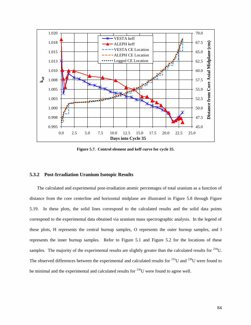
84
Figure 5.7. Control element and keff curve for cycle 35.
5.3.2 Post-Irradiation Uranium Isotopic Results
The calculated and experimental post-irradiation atomic percentages of total uranium as a function of
distance from the core centerline and horizontal midplane are illustrated in Figure 5.8 through Figure
5.19. In these plots, the solid lines correspond to the calculated results and the solid data points
correspond to the experimental data obtained via uranium mass spectrographic analysis. In the legend of
these plots, H represents the central burnup samples, O represents the outer burnup samples, and I
represents the inner burnup samples. Refer to Figure 5.1 and Figure 5.2 for the locations of these
samples. The majority of the experimental results are slightly greater than the calculated results for 234
U.
The observed differences between the experimental and calculated results for 235
U and 238
U were found to
be minimal and the experimental and calculated results for 236
U were found to agree well.
45.0
47.5
50.0
52.5
55.0
57.5
60.0
62.5
65.0
67.5
70.0
0.995
0.998
1.000
1.003
1.005
1.008
1.010
1.013
1.015
1.018
1.020
0.0 2.5 5.0 7.5 10.0 12.5 15.0 17.5 20.0 22.5 25.0
Dis
tan
ce f
rom
Co
re A
xia
l M
idp
lan
e (c
m)
kef
f
Days into Cycle 35
VESTA keff
ALEPH keff
VESTA CE Location
ALEPH CE Location
Logged CE Location

85
The OFE is studied for cycles 4 and 16 and the OFE is surrounded by the IFE and a water channel to
its inside, water on top of and below it, and the control region and the beryllium reflector to its outside.
The effects from these regions are apparent in the plots for cycles 4 and 16. The most depleted (least
amount of post-irradiation 235
U) region is the outer edge of the OFE at the horizontal midplane and this is
because the water and beryllium regions to the outside of the OFE moderate fast neutrons that leak from
the OFE and reflect them back into the OFE as thermal neutrons. The IFE is studied in cycle 35 and the
IFE is surrounded by the flux trap to its inside, a water channel and the OFE to its outside and water on
top of and below it. The most depleted region in the IFE occurs at the inner edge of the plates at
horizontal midplane and this is because fast neutrons leak from the IFE region into the flux trap, which
moderates fast neutrons and reflects them back into the IFE as thermal neutrons.
Figure 5.8. Cycle 4 OFE post-irradiation 234
U atomic percent.
-30
-25
-20
-15
-10
-5
0
5
10
15
20
25
30
0.95% 1.00% 1.05% 1.10% 1.15% 1.20% 1.25% 1.30% 1.35%
Dis
tan
ce F
rom
Core
Axia
l M
idp
lan
e (c
m)
Post-Irradiation U-234/Uranium at. %
Meas. (I) VESTA (I) ALEPH (I)
Meas. (H) VESTA (H) ALEPH (H)
Meas. (O) VESTA (O) ALEPH (O)

86
Figure 5.9. Cycle 4 OFE post-irradiation 235
U atomic percent.
Figure 5.10. Cycle 4 OFE post-irradiation 236
U atomic percent.
-30
-25
-20
-15
-10
-5
0
5
10
15
20
25
30
75.0% 77.5% 80.0% 82.5% 85.0% 87.5% 90.0% 92.5%
Dis
tan
ce F
rom
Co
re A
xia
l M
idp
lan
e(c
m)
Post-Irradiation U-235/Uranium at. %
Meas. (I) VESTA (I) ALEPH (I)
Meas. (H) VESTA (H) ALEPH (H)
Meas. (O) VESTA (O) ALEPH (O)
-30
-25
-20
-15
-10
-5
0
5
10
15
20
25
30
2.0% 4.0% 6.0% 8.0% 10.0% 12.0% 14.0%
Dis
tan
ce F
rom
Co
re A
xia
l M
idp
lan
e (c
m)
Post-Irradiation U-236/Uranium at. %
Meas. (I) VESTA (I) ALEPH (I)
Meas. (H) VESTA (H) ALEPH (H)
Meas. (O) VESTA (O) ALEPH (O)
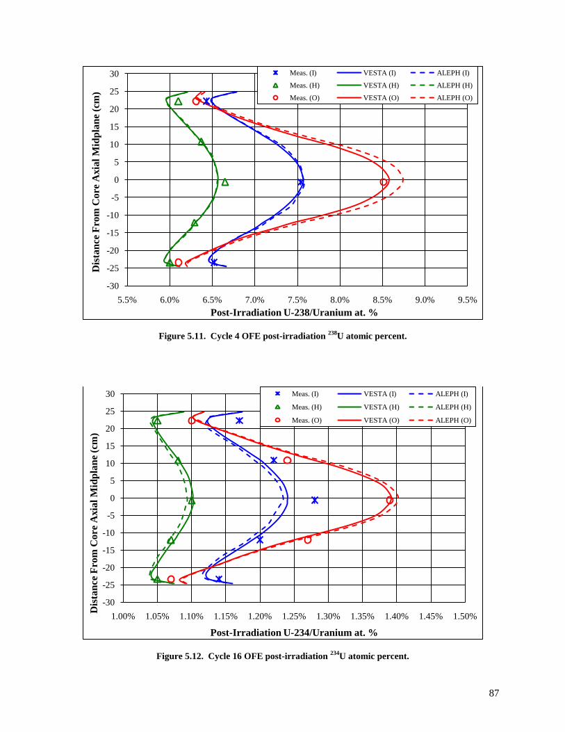
87
Figure 5.11. Cycle 4 OFE post-irradiation 238
U atomic percent.
Figure 5.12. Cycle 16 OFE post-irradiation 234
U atomic percent.
-30
-25
-20
-15
-10
-5
0
5
10
15
20
25
30
5.5% 6.0% 6.5% 7.0% 7.5% 8.0% 8.5% 9.0% 9.5%
Dis
tan
ce F
rom
Co
re A
xia
l M
idp
lan
e (c
m)
Post-Irradiation U-238/Uranium at. %
Meas. (I) VESTA (I) ALEPH (I)
Meas. (H) VESTA (H) ALEPH (H)
Meas. (O) VESTA (O) ALEPH (O)
-30
-25
-20
-15
-10
-5
0
5
10
15
20
25
30
1.00% 1.05% 1.10% 1.15% 1.20% 1.25% 1.30% 1.35% 1.40% 1.45% 1.50%
Dis
tan
ce F
rom
Co
re A
xia
l M
idp
lan
e (c
m)
Post-Irradiation U-234/Uranium at. %
Meas. (I) VESTA (I) ALEPH (I)
Meas. (H) VESTA (H) ALEPH (H)
Meas. (O) VESTA (O) ALEPH (O)
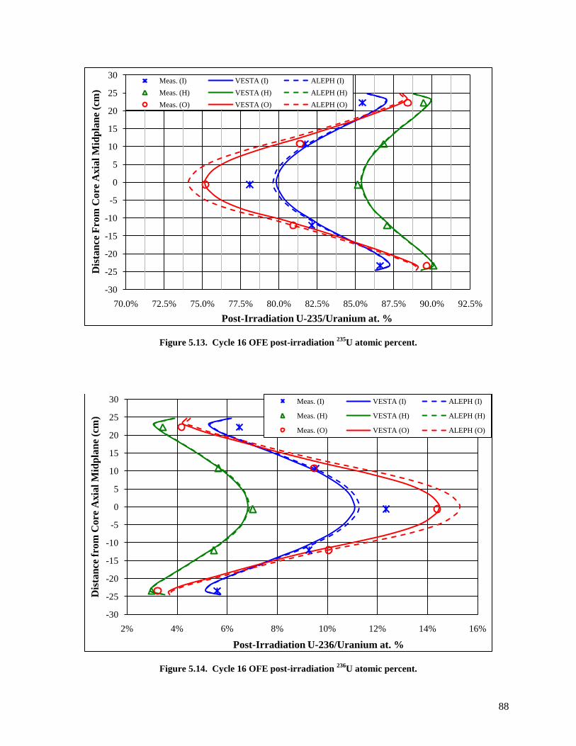
88
Figure 5.13. Cycle 16 OFE post-irradiation 235
U atomic percent.
Figure 5.14. Cycle 16 OFE post-irradiation 236
U atomic percent.
-30
-25
-20
-15
-10
-5
0
5
10
15
20
25
30
70.0% 72.5% 75.0% 77.5% 80.0% 82.5% 85.0% 87.5% 90.0% 92.5%
Dis
tan
ce F
rom
Co
re A
xia
l M
idp
lan
e (c
m)
Post-Irradiation U-235/Uranium at. %
Meas. (I) VESTA (I) ALEPH (I)
Meas. (H) VESTA (H) ALEPH (H)
Meas. (O) VESTA (O) ALEPH (O)
-30
-25
-20
-15
-10
-5
0
5
10
15
20
25
30
2% 4% 6% 8% 10% 12% 14% 16%
Dis
tan
ce f
rom
Co
re A
xia
l M
idp
lan
e (c
m)
Post-Irradiation U-236/Uranium at. %
Meas. (I) VESTA (I) ALEPH (I)
Meas. (H) VESTA (H) ALEPH (H)
Meas. (O) VESTA (O) ALEPH (O)
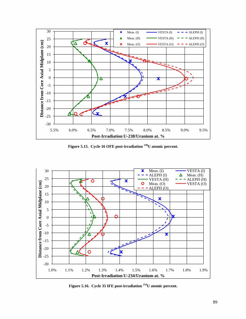
89
Figure 5.15. Cycle 16 OFE post-irradiation 238
U atomic percent.
Figure 5.16. Cycle 35 IFE post-irradiation 234
U atomic percent.
-30
-25
-20
-15
-10
-5
0
5
10
15
20
25
30
5.5% 6.0% 6.5% 7.0% 7.5% 8.0% 8.5% 9.0% 9.5%
Dis
tan
ce f
rom
Co
re A
xia
l M
idp
lan
e (c
m)
Post-Irradiation U-238/Uranium at. %
Meas. (I) VESTA (I) ALEPH (I)
Meas. (H) VESTA (H) ALEPH (H)
Meas. (O) VESTA (O) ALEPH (O)
-30
-25
-20
-15
-10
-5
0
5
10
15
20
25
30
1.0% 1.1% 1.2% 1.3% 1.4% 1.5% 1.6% 1.7% 1.8% 1.9%
Dis
tan
ce f
rom
Co
re A
xia
l M
idp
lan
e (c
m)
Post-Irradiation U-234/Uranium at. %
Meas. (I) VESTA (I)ALEPH (I) Meas. (H)VESTA (H) ALEPH (H)Meas. (O) VESTA (O)ALEPH (O)

90
Figure 5.17. Cycle 35 IFE post-irradiation 235
U atomic percent.
Figure 5.18. Cycle 35 IFE post-irradiation 236
U atomic percent.
-30
-25
-20
-15
-10
-5
0
5
10
15
20
25
30
55% 60% 65% 70% 75% 80% 85% 90%
Dis
tan
ce F
rom
Co
re A
xia
l M
idp
lan
e (c
m)
Post-Irradiation U-235/Uranium at. %
Meas. (I) VESTA (I) ALEPH (I)
Meas. (H) VESTA (H) ALEPH (H)
Meas. (O) VESTA (O) ALEPH (O)
-30
-25
-20
-15
-10
-5
0
5
10
15
20
25
30
2.5% 7.5% 12.5% 17.5% 22.5% 27.5% 32.5%
Dis
tan
ce f
rom
Core
Axia
l M
idp
lan
e (c
m)
Post-Irradiation U-236/Uranium at. %
Meas. (I) VESTA (I) ALEPH (I)
Meas. (H) VESTA (H) ALEPH (H)
Meas. (O) VESTA (O) ALEPH (O)

91
Figure 5.19. Cycle 35 IFE post-irradiation 238
U atomic percent.
5.3.3 Fissile and Neutron Poison Nuclide Inventory
The results in this section correspond to the cycle 16 ALEPH calculation. The initial amount of 235
U
in a HFIR unirradiated core is approximately 9.4 kilograms. For cycle 16, a total of 9.404 kilograms of
235U was modeled as the beginning-of-life
235U inventory, which is within the allowed uncertainty. At the
end-of-cycle 16 (2309 MWd), a sum of 6.49 kilograms of 235
U remained in the core, which is 69 % of the
initial 235
U. Thus, only 31 % of the total uranium was burned and an average burnup of about 245.5
MWd per kilogram initial 235
U was achieved. As irradiation time increases and the 235
U inventory
decreases, 239
Pu builds in by neutron capture from 238
U. Plutonium-239 is a fissile nuclide that is
accountable for approximately 6 % of total fissions at the end of a typical HFIR fuel cycle [23]. The
depletion of 235
U and the buildup of 239
Pu as a function of core exposure for cycle 16 are illustrated in
Figure 5.20.
-30
-25
-20
-15
-10
-5
0
5
10
15
20
25
30
6% 7% 8% 9% 10% 11% 12% 13%
Dis
tan
ce f
rom
Co
re A
xia
l M
idp
lan
e (c
m)
Post-Irradiation U-238/Uranium at. %
Meas. (I) VESTA (I) ALEPH (I)
Meas. (H) VESTA (H) ALEPH (H)
Meas. (O) VESTA (O) ALEPH (O)

92
Figure 5.20. 235
U depletion and 239
Pu buildup as a function of exposure for HFIR cycle 16.
Xenon-135 and 149
Sm account for over 90 % of fission product poisoning in the HFIR core, and
therefore, must be tracked during depletion calculations. Xenon-135 and 149
Sm have thermal neutron
absorption cross sections of about 2.6x10⁶ and 4.1x10
4 barns, respectively, and therefore introduce large
amounts of negative reactivity into the HFIR core. The concentration of 135
Xe rapidly increases and
reaches an equilibrium concentration of about 0.075 grams in the HFIR core at approximately 175 MWd
(1.75 days at 100 MW) and then decreases to about 0.051 grams. This 31 % decrease in equilibrium
xenon, which should theoretically remain constant, is thought to be due to the consumption of 235
U and
the spatial/spectral effects as a function of exposure in HFIR [23]. The 149
Sm concentration reaches
equilibrium at about 0.40 grams at approximately 1000 MWd (10 days at 100 MW) and decreases to
about 0.36 grams at end-of-life. The 10 % decrease in equilibrium 149
Sm, which should theoretically
remain constant, is due to the consumption of 235
U and an increase in thermal flux at EOC [23]. The
buildup of 135
Xe and 149
Sm as a function of exposure for cycle 16 is shown in Figure 5.21.
0
1
2
3
4
5
6
7
8
9
10
11
12
13
6.25
6.50
6.75
7.00
7.25
7.50
7.75
8.00
8.25
8.50
8.75
9.00
9.25
9.50
0 200 400 600 800 1000 1200 1400 1600 1800 2000 2200 2400
Plu
ton
ium
-23
9 I
nv
ento
ry (
gra
ms)
Ura
niu
m-2
35
In
ven
tory
(k
ilo
gra
ms)
Core Exposure (MWd)
U-235
Pu-239

93
Figure 5.21. 135
Xe and 149
Sm buildup as a function of exposure for HFIR cycle 16.
Boron-10 in a mixture of B4C is used as a burnable poison and is nonuniformly distributed along the
arc of the IFE fuel plates. The mixture is dispensed in the aluminum filler, which is separate from the fuel
region. The radial distribution of the burnable poison in the IFE fuel plates was chosen to limit the
maximum-to-average power density ratio (qmax/qavg) and to minimize the 235
U burnup at the edges of the
fuel plates. The initial 10
B loading in the HFIR core is 2.8 grams, which amounts to about 16.4
milligrams per IFE fuel plate. According to the ALEPH calculation, approximately 0.16 grams of 10
B
remained in the core following the discharge of cycle 16 (2309 MWd). Thus, approximately 94 % of the
initial 10
B was depleted. The total IFE 10
B inventory as a function of exposure for cycle 16 is shown in
Figure 5.22.
0.00
0.01
0.02
0.03
0.04
0.05
0.06
0.07
0.08
0.09
0.00
0.05
0.10
0.15
0.20
0.25
0.30
0.35
0.40
0.45
0 200 400 600 800 1000 1200 1400 1600 1800 2000 2200 2400
Xen
on
-13
5 I
nv
ento
ry (
gra
ms)
Sa
ma
riu
m-1
49
In
ven
tory
(g
ram
s)
Core Exposure (MWd)
Sm-149
Xe-135

94
Figure 5.22. 10
B inventory as a function of exposure for HFIR cycle 16.
5.4 Post-Irradiation Inventory Summary
HFIR fuel cycles 4, 16, and 35 were modeled using ALEPH and VESTA to calculate the post-
irradiation isotopic atomic percentages of the uranium isotopes. In order to validate the Monte Carlo-
based depletion methodology described in this chapter, the calculated results were compared against
measured results that were obtained from uranium mass spectrographic analysis. Good agreement was
observed between the calculated and measured results, which reveal that both ALEPH and VESTA can be
used to accurately calculate the burnup dependent uranium inventory of the HFIR core. No trends were
found while examining the C/E ratios as a function of radial or axial location, and thus, it was determined
that a bias factor is not needed for current fuel design studies.
For all three cycles modeled, the calculated post-irradiation 235
U atomic percentages agreed best with
the experimental data. The majority of the 234
U C/E ratios were less than unity, and thus, it is postulated
0.00
0.25
0.50
0.75
1.00
1.25
1.50
1.75
2.00
2.25
2.50
2.75
3.00
0 200 400 600 800 1000 1200 1400 1600 1800 2000 2200 2400
Bo
ron
-10
IF
E I
nv
ento
ry (
gra
ms)
Core Exposure (MWd)
B-10
95
that the 234
U capture cross section and/or the 235
U (n,2n) cross section may be too low. However, since no
uncertainties are available for the measured data, it is not rational to declare that these cross sections are
too low. The errors associated with calculating the 234
U content (or the other uranium isotopic
concentrations) causes errors in the other isotopes since atomic percentages are being calculated (i.e.,
atomic percentages are interdependent). However, if a 5 % uncertainty was applied to the experimental
results (a value noted in [69] as applicable to local power density determinations based on fission product
gamma activity), 93 % of the calculated 234
U atomic densities, 56 % of the 236
U atomic densities, and 100
% of the 235
U and 238
U atomic densities would fall within the experimental uncertainty range.
The precise calculation of the 235
U distribution proves that the methodology described in this report
could be used to accurately calculate the power distribution variation as a function of space and time
(burnup) for the HFIR reactor fuelled with HEU. Chapter 4 documents power distribution comparisons
between experimental and calculated results for two different scenarios: a clean core condition (control
elements withdrawn 44.536 cm), which simulates BOC, and a poisoned core condition (control elements
fully withdrawn and 1.35 grams of boron per liter in the moderator), which simulates EOC. The boron in
the moderator was used to simulate fission product poisons present at EOC. The results from Chapter 4
were insightful, but provided power distributions for unirradiated fuel conditions (i.e., not burnup
dependent). This study, however, provided burnup dependent cases which are important because the
spatial power distribution in HFIR changes significantly during the cycle due to the control element
movement. Therefore, this study proves that the power distribution can be accurately calculated as a
function of irradiation time, and thus, time dependent power profiles needed for reactor core thermal
hydraulic and reactor kinetics analyses, if derived from this methodology, have been shown to be accurate
for HEU fuel.
The methodology described in this chapter was also used for a feasibility study used to assess the
production of plutonium-238 in the VXF facilities located in the beryllium reflector. The study is briefly
documented in Appendix B.
96
6 Beryllium Activation Impacts on Startup and Reflector Disposal
HFIR utilizes a large annular beryllium reflector that is subdivided into three concentric regions and
encompasses the compact reactor core. Nuclear transmutations caused by neutron activation occur in the
beryllium reflector regions, which leads to unwanted neutron absorbing and radiation emitting isotopes.
Two topics related to the HFIR beryllium reflector are presented in this chapter. The first topic includes
studying the neutron poison (helium-3 and lithium-6) buildup in the reflector regions and its effect on
beginning-of-cycle reactivity. The second topic includes studying the composition of the beryllium
reflector regions at discharge as well as during post-discharge decay to assess the viability of transporting,
storing, and ultimately disposing of the reflector regions currently stored in the spent fuel pool. The post-
irradiation curie inventories are used to determine whether, for disposal purposes, the reflector regions are
discharged as transuranic waste or become transuranic waste during the decay period and to determine the
nuclear hazard category, which may affect the controls invoked for transportation and temporary storage.
6.1 Beryllium Activation Effects
Two topics related to the beryllium reflector are being studied. The first topic includes studying the
poison (3He and
6Li) buildup in the reflector regions and its effect on beginning-of-cycle (BOC) reactivity
and the startup symmetrical critical control element positions. A reactivity difference of $1.55, which is
approximately equal to 0.5 inches in control element position at startup, is the maximum reactivity
difference allowed at startup and if exceeded, a technical evaluation is performed to resolve the
discrepancy prior to a restart. After a 484 day outage following cycle 407 (Jan. 2006 to May 2007), the
reactivity attributed to 3He was erroneously calculated using the current methodology. This occurrence is
the motivation for developing a new methodology to predict the reactivity impact 3He has on reactor
startup following long outages. This study will be referred to as study number 1 for the duration of this
chapter.
97
The second topic includes studying the composition of the beryllium reflector regions at discharge as
well as during post-discharge decay to assess the viability of transporting, storing, and ultimately
disposing of the reflector regions currently stored in the HFIR spent fuel pool. The post-irradiation curie
inventories determine whether the reflector regions are discharged as transuranic waste, become
transuranic waste during some period of decay or are not transuranic waste. Categorization is necessary
for determination of path to disposal and to establish the nuclear hazard category; the category
designation affects the controls invoked for transportation and temporary storage. This topic is
subdivided into two studies, which will be referred to as study number 2 and study number 3 for the
duration of this chapter.
Study number 2 was initially performed to determine whether the permanent beryllium reflector
number 3 (PB3) currently exceeds the transuranic (TRU) waste threshold and whether typical RB and
SPB reflectors are discharged as or subsequently become TRU waste. Study number 3 was performed to
determine the total curie inventory in PB3 and representative RB and SPB reflectors at discharge and
during decay. The methods used in study number 2 are similar to study number 3, with the main
differences being that study number 3 used a much more detailed material composition in the reflector
because study number 2 was performed to determine the transuranic inventory and study number 3 was
performed to determine the total radionuclide inventory.
6.1.1 Nuclear Transmutations Caused by Neutron Activation
The main disadvantage of using beryllium in a neutron environment is the buildup of helium and
hydrogen isotopes. Helium-3 is a neutron poison (absorber) that also causes swelling and mechanical
property changes, 4He is a gas that also leads to swelling, and tritium (
3H) is a radionuclide that has the
potential to be released. Beryllium reflectors must be replaced periodically due to the internal stresses
that are caused by swelling generated by helium and hydrogen gases [82].

98
When 9Be is irradiated by neutrons above ~1 MeV, it undergoes (n,α) and (n,2n) reactions [82].
Beryllium-9 can also undergo (n,γ) reactions when irradiated by thermal neutrons. The reaction that
causes poisoning is the (n,α) reaction that leads to the buildup of 6Li and
3He; two isotopes with large
thermal absorption cross sections. Thus, a negative reactivity is introduced in the reflector, which has to
be accounted in order to accurately predict the startup positions of control elements. The nuclear
reactions that govern the transmutations and lead to poisoning are defined in Equation 6.1 through
Equation 6.7.
Equation 6.1
Equation 6.2
Equation 6.3
Equation 6.4
Equation 6.5
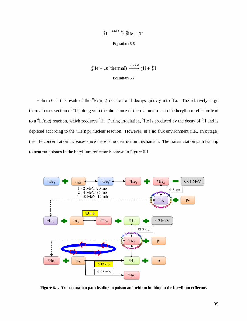
99
Equation 6.6
Equation 6.7
Helium-6 is the result of the 9Be(n,α) reaction and decays quickly into
6Li. The relatively large
thermal cross section of 6Li, along with the abundance of thermal neutrons in the beryllium reflector lead
to a 6Li(n,α) reaction, which produces
3H. During irradiation,
3He is produced by the decay of
3H and is
depleted according to the 3He(n,p) nuclear reaction. However, in a no flux environment (i.e., an outage)
the 3He concentration increases since there is no destruction mechanism. The transmutation path leading
to neutron poisons in the beryllium reflector is shown in Figure 6.1.
Figure 6.1. Transmutation path leading to poison and tritium buildup in the beryllium reflector.
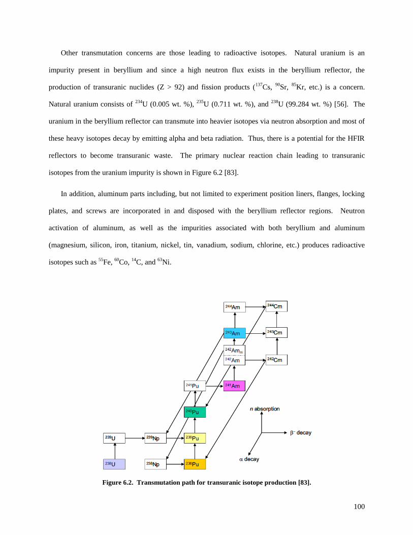
100
Other transmutation concerns are those leading to radioactive isotopes. Natural uranium is an
impurity present in beryllium and since a high neutron flux exists in the beryllium reflector, the
production of transuranic nuclides (Z > 92) and fission products (137
Cs, 90
Sr, 85
Kr, etc.) is a concern.
Natural uranium consists of 234
U (0.005 wt. %), 235
U (0.711 wt. %), and 238
U (99.284 wt. %) [56]. The
uranium in the beryllium reflector can transmute into heavier isotopes via neutron absorption and most of
these heavy isotopes decay by emitting alpha and beta radiation. Thus, there is a potential for the HFIR
reflectors to become transuranic waste. The primary nuclear reaction chain leading to transuranic
isotopes from the uranium impurity is shown in Figure 6.2 [83].
In addition, aluminum parts including, but not limited to experiment position liners, flanges, locking
plates, and screws are incorporated in and disposed with the beryllium reflector regions. Neutron
activation of aluminum, as well as the impurities associated with both beryllium and aluminum
(magnesium, silicon, iron, titanium, nickel, tin, vanadium, sodium, chlorine, etc.) produces radioactive
isotopes such as 55
Fe, 60
Co, 14
C, and 63
Ni.
Figure 6.2. Transmutation path for transuranic isotope production [83].

101
6.1.2 Startup Procedure
HFIR fuel cycle 407 ended on January 13, 2006 and cycle 408 began on May 13, 2007. The 484 day
outage was due to the conversion of horizontal beam tube number four from a 30-m small angle neutron
scattering facility to a high performance hydrogen cold source. The estimated symmetrical critical
control element position (ESCCEP) for the startup of cycle 408 was 18.656 inches [84]. During the
startup of cycle 408, the difference between the estimated and actual symmetrical positions exceeded
$1.55 requiring a pause in reactor startup. If the reactivity difference between actual and calculated
startup equals or exceeds $1.55, approximately equal to 0.5 inches in control element position at startup,
the startup procedure is suspended and a technical evaluation is performed to resolve the discrepancy
prior to a restart. Following the pause in the approach to critical, the ESCCEP was reexamined and it was
determined that the reactivity attributed to shutdown 3He poison was too large using the current
methodology.
The actual symmetrical critical control element position (ASCCEP) for the startup of cycle 408 was
18.090 inches, a difference of 0.566 inches from the estimated startup position. The incorrect prediction
of the ASCCEP for cycle 408 due to an incorrect prediction in the 3He poisoning effect is the motivation
behind developing a better 3He poisoning correlation. Helium-3 buildup effects have been studied for
other beryllium reflected reactors such as the MARIA reactor at the Institute of Atomic Energy in Poland
[85] and the Belgium Reactor 2 (BR2) located at SCK-CEN in Belgium [86].
The current methodology for calculating the change in symmetrical critical control element position
with respect to a reference cycle, typically the cycle prior to the current cycle (ΔR), associated with 3He
buildup is shown in Equation 6.8 where Td,C is the decay time on the reflector for the current cycle
(outage time between the shutdown of previous cycle and the startup of the current cycle) and Td,R is the
decay time on the reflector for the previous cycle. The value 0.0047 is a multiplicative factor used to
convert from decay time to change in control element position and was obtained for the reactor when it
operated at 100 MWth and is based on measurements obtained for typical outages during the late 1960s (a
102
couple days to a month). If the current decay time is greater than the reference decay time the ΔR value is
positive and the control elements are withdrawn (due to a larger, 3He induced, negative reactivity) and
vice versa.
ΔR (inches) = 0.0047 (inches/day) [Td,C (days) - Td,R(days)]
Equation 6.8
6.1.3 Beryllium Waste Concerns
It is desired to move beryllium reflectors that have been discharged from the reactor out of their
interim storage location in the spent fuel pool to make room for anticipated operational and maintenance
activities. Once the Be reflectors are declared as waste, they must be characterized to ensure safe interim
storage and to facilitate eventual disposal. As part of the characterization process, the isotopic inventory
of radiological constituents in the reflectors must be determined. The curie inventory of identified
isotopes is compared against the acceptance criteria of potential waste storage and disposal sites to
determine whether the waste may be received and stored at the sites. The inventory also defines the
nuclear hazard category which is used in defining hazard controls in associated safety documentation for
transportation and storage.
The reflectors are currently designated as ―waste with no identified path to disposal‖ under DOE
Order 435.1, [87] and [88], which specifies requirements for managing radioactive waste generated by
DOE activities. DOE Order 435.1 requires that efforts be made to define an acceptable disposal option
for waste that has been designated as having no identified disposal path. The reflectors were originally
classified as having no identified disposal path based on a conservative characterization that indicated the
curie inventory of selected isotopes would exceed the waste acceptance criteria for the Nevada Test Site,
the expected disposal location. Since that time, studies of the beryllium reflector utilized in the Advanced

103
Test Reactor (ATR) located at the Idaho National Laboratory (INL) have shown that reflectors used in the
ATR will exceed the threshold for transuranic (TRU) waste because of trace uranium impurities in the
beryllium [83]. Previous analyses have indicated that the HFIR reflectors may also satisfy the definition
of TRU waste [89] because of similar levels of trace uranium initially in the beryllium base metal.
Studies reported here were intended to confirm or refute the TRU waste characterization.
The current specification for the HFIR beryllium reflectors requires the uranium content to be less
than 0.0011 weight percent (11 micrograms of uranium per gram of reflector), but previous HFIR
reflectors have been fabricated with a greater uranium content (as much as 0.0044 weight percent). The
Nevada Test Site Waste Acceptance Criteria [90] defines TRU waste as radioactive waste containing
more than 100 nCi (3700 Bq) of alpha-emitting transuranic nuclides (Z > 92) with half-lives greater than
20 years per gram of waste. Therefore, the following nuclides are considered when making the TRU
waste determination: 237
Np, 238
Pu, 239
Pu, 240
Pu, 242
Pu, 244
Pu, 241
Am, 242m
Am, 243
Am, 243
Cm, 245
Cm, 246
Cm,
247Cm,
248Cm,
250Cm,
247Bk,
249Cf, and
251Cf. Using this criterion, the presence and quantity of applicable
transuranic nuclides in the HFIR reflectors was evaluated at discharge and as a function of decay time for
making the TRU waste determination.
In order to move HFIR reflectors from their current location to a new storage site, the degree of
nuclear hazard associated with the reflectors must be determined in accordance with DOE-STD-1027
[91]. The post-irradiation isotopic inventory and curie levels in the reflector are used to determine the
nuclear hazard category. This standard defines three hazard categories based on isotopic thresholds using
a sum-of-the-fractions approach. The threshold for hazard category 3 was designed to include facilities
and activities that under-postulated accident conditions may have no more than localized radiological
consequences. Postulated accidents involving a hazard category 2 inventory have the potential for
significant on-site radiological consequences and accidents involving a hazard category 1 inventory can
result in significant off-site consequences.

104
6.2 Computational Methodology
Version 6.0 of the SCALE package [56] was the primary code utilized for these studies. Three-
dimensional KENO V.a and KENO-VI models of the HFIR [8] were used for multi-material depletion
calculations. TRITON was used to couple the Monte Carlo transport code KENO to the point depletion
code ORIGEN-S. For a few cases, in order to extend the TRITON results with larger numbers of
histories and different random number sequences, the TRITON results were appended through the use of
the SCALE CSAS module, a criticality safety analysis code. For all SCALE calculations, the 238-group
ENDF/B-VII cross section library was used.
As a quality assurance check of the TRITON-related model development, "stand-alone" ORIGEN
calculations were performed. A benchmarked three-dimensional MCNP5 model [24] along with
continuous energy ENDF/B-VI.8 data was used to calculate the three-group fluxes required in stand-alone
ORIGEN-S calculations. The time-dependent MCNP5 inputs used were generated by ALEPH [54]. The
KENO models used in these studies were developed based on the benchmarked/validated HFIR cycle 400
MCNP model and were benchmarked against this MCNP model in [8] - [13] for various parameters such
as flux magnitude, flux spectra, keff, and etc.
The KENO input was set up such that the RB was subdivided into 3 radial regions, the SPB was
modeled as one radial region, and the PB was subdivided into 7 radial regions in order to utilize a radially
dependent flux distribution since the neutron flux decreases with increasing penetration of the reflectors.
An isometric view of the KENO model is shown in Figure 6.3.

105
Figure 6.3. Isometric view of the HFIR KENO model.
6.2.1 Startup Reactivity Effects Methodology
A typical HFIR cycle consists of 25 days of irradiation followed by 25 days of outage time between
cycles. For this study, 20 typical cycles were modeled with each cycle consisting of a 25 day irradiation
period at 85 MWth (~8423 MW/MTIHM) and 25 days of down time, td. Another 25 day irradiation step
was simulated after the 20 cycles, and following the end of the 21st irradiation step, multiple decay steps
(3, 6, 12, 24, 48, 96, 192, 384, 492, 611, and 730 days) were defined. The first 20 cycles were modeled to
allow for poison buildup and were chosen such that equilibrium 6Li would be reached.
The compositions of the reflector regions at beginning-of-cycle (BOC) 21 and following each of the
decay steps (i.e., BOC 22 reflector compositions) were extracted and inserted into CSAS5 inputs, which
were used for static keff calculations. The BOC 21 keff was calculated for the ―reference‖ case and the
BOC 22 keff values (based on the composition following the decay steps) were calculated in order to

106
determine a correlation attributed to shutdown poisons as a function of td. Although the effective
multiplication factors could have been taken out of the TRITON output, it was desired to increase the
number of histories to obtain better statistics. Ten million histories per transport calculation were
simulated in the TRITON/KENO run since numerous transport calculations were performed, but 50
million histories were simulated in the CSAS5/KENO runs. The geometry and material compositions,
except for the reflector’s composition, were the same for both the CSAS5 and TRITON inputs. Test
cases utilizing up to 50 million histories per step were run in TRITON and no significant compositional or
flux differences in the reflector regions were observed.
The keff values were extracted from the CSAS5 outputs and were used to calculate the Δkeff/keff (%)
values (reactivity effect of 3He as a function of td) using Equation 6.9. These values were then converted
into Δρ ($) values (change in reactivity) by dividing by 0.00762, the delayed neutron fraction (βeff)
associated with HFIR [29]. The corresponding ΔR values were obtained by utilizing the ―typical‖ startup
position control element worth of $3.10/inch.
Equation 6.9
6.2.2 Waste Classifications Methodology
Activation calculations were performed on the HFIR beryllium reflector regions in order to
characterize them so HFIR staff could assess the viability of moving them out of the spent fuel pool.
Study number 2 was performed to determine whether the permanent beryllium reflector number 3 (PB3)
currently exceeds the TRU waste threshold and whether typical RB and SPB reflectors are discharged as
or subsequently become TRU waste. Study number 3 was performed to determine the total curie
inventory in PB3 and representative RB and SPB reflectors at discharge and during decay.

107
At the time the calculations in study number 2 were performed, the goal was to calculate the TRU
inventory. The beryllium reflectors were modeled as solid beryllium cylinders containing uranium and
impurities based on neutron activation analyses (NAA) on three in-vessel non-reflector beryllium
components. The uranium concentration in PB3 was known to be 0.0044 weight percent, which was used
along with the NAA results for the other beryllium impurities. The PB3 design file [92] was located by
HFIR staff and the material composition contained therein was used in study number 3 to calculate the
post-irradiation curie contributing inventory. The uranium concentration listed in [92] is 0.0044 weight
percent, which was the value used in both study numbers 2 and 3.
The TRU inventory for PB3 and representative RB and SPB reflectors was initially calculated
utilizing TRITON/KENO V.a. A separate calculation was performed for each of the three reflector
regions. The KENO radial flux results in the reflector were compared to benchmarked ALEPH/MCNP
[77] time-dependent results and were shown to be slightly larger and therefore slightly conservative since
the reflector regions were depleted by flux (Figure 6.4). The KENO fluxes are slightly greater because
the fuel in the TRITON model is not depleted and poison is uniformly distributed in the control element
channel. With the resources available, it was not feasible to deplete the fuel and simulate control element
movement for 138 cycles. Comparisons over single cycles showed that the perturbations in flux
magnitude and spectra are small when compared to time-dependent ALEPH/MCNP calculations where
both fuel depletion and control element movement are modeled (Figure 6.4).
PB3 was inserted into HFIR between cycles 244 and 245 (cycle 245 began on Jan. 1, 1984) and was
removed following the end of cycle 382 (Oct. 1, 2000). HFIR experienced an outage for 3.5 years
between cycles 287 and 288 while reactor vessel embrittlement concerns were addressed. The outcome
of the outage, which occurred between November 14, 1986 and May 18, 1990, was a power decrease
from 100 MWth to 85 MWth. Thus, the calculation performed in order to characterize PB3 utilized 4
steps: (1) irradiate at 100 MW for 926.5 days (92646 MWd), (2) decay for 1280 days, (3) irradiate at 85
MW for 2,204 days (187341 MWd), and (4) post-discharge decay, [89] and [93].
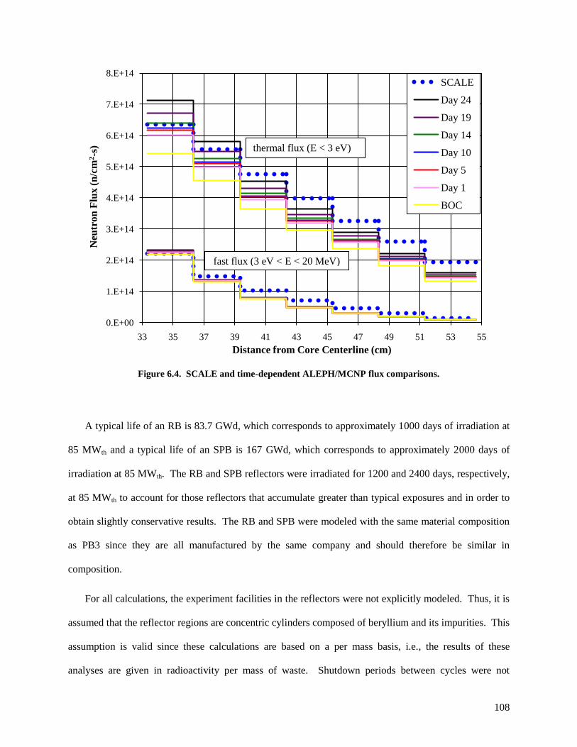
108
Figure 6.4. SCALE and time-dependent ALEPH/MCNP flux comparisons.
A typical life of an RB is 83.7 GWd, which corresponds to approximately 1000 days of irradiation at
85 MWth and a typical life of an SPB is 167 GWd, which corresponds to approximately 2000 days of
irradiation at 85 MWth. The RB and SPB reflectors were irradiated for 1200 and 2400 days, respectively,
at 85 MWth to account for those reflectors that accumulate greater than typical exposures and in order to
obtain slightly conservative results. The RB and SPB were modeled with the same material composition
as PB3 since they are all manufactured by the same company and should therefore be similar in
composition.
For all calculations, the experiment facilities in the reflectors were not explicitly modeled. Thus, it is
assumed that the reflector regions are concentric cylinders composed of beryllium and its impurities. This
assumption is valid since these calculations are based on a per mass basis, i.e., the results of these
analyses are given in radioactivity per mass of waste. Shutdown periods between cycles were not
0.E+00
1.E+14
2.E+14
3.E+14
4.E+14
5.E+14
6.E+14
7.E+14
8.E+14
33 35 37 39 41 43 45 47 49 51 53 55
Neu
tro
n F
lux (
n/c
m2-s
)
Distance from Core Centerline (cm)
SCALE
Day 24
Day 19
Day 14
Day 10
Day 5
Day 1
BOC
thermal flux (E < 3 eV)
fast flux (3 eV < E < 20 MeV)

109
modeled, except for the 3.5 year shutdown between cycles 287 and 288 (applicable for PB3 model only).
The difference in continual irradiation versus operating cycles (~25 days of irradiation, ~25 days of
outage, . . .) adds conservatism in that actual decay periods between operating cycles are not modeled.
Thus, the curie levels calculated in the reflector by not modeling outages are greater than the curie levels
that would be calculated if the outages were modeled.
Control element withdrawal and fuel burnup was not simulated and the reactor power was kept at a
constant value of 85 MWth (100 MWth for the first ~3 years of PB3 analysis). The power distribution
within the core could affect local TRU isotopic concentrations but the total inventory of TRU products in
the reflector will be largely unaffected. Only the core leakage spectra and magnitude are important in
these calculations of TRU products, not the details of what is happening inside the fuelled region.
Therefore, each of the reflector regions was modeled as one axial zone. However, they were modeled as
multiple radial regions, such that a different flux is utilized in each separate region.
Calculations were performed in study 3 to determine the total curie inventory in PB3, an RB, and an
SPB at discharge and during decay. The design file for PB3 [92], which lists the chemical composition of
the reflector (beryllium and impurities) as determined by chemical and neutron activation analyses, was
utilized for determining the initial reflector nuclide inventory. The Al-6061 parts (experiment position
liners, locking plates, etc.) and the 321 stainless steel (SST) O-rings were included in PB3 by distributing
their constituents uniformly throughout the beryllium reflector. The 321 SST composition was retrieved
from [89], which lists the AISI composition limits. The chemical composition of the Al-6061 was chosen
based on the most conservative mixture determined in [94], a report in which a beryllium experiment
facility composed of six different compositions (6 different calculations) was analyzed.
TRITON was again used to couple KENO and ORIGEN-S, but for these studies KENO-VI was
utilized. A HFIR KENO-VI model was constructed after performing study number 2 solely because the
geometry package in KENO-VI is more flexible than that in KENO V.a. The same irradiation history as
described in previous paragraphs was used to deplete PB3.

110
Due to 1) the desire by management to compare the current results with previous similar studies [89]
utilizing stand-alone ORIGEN-S calculations and 2) the computational time required to run these
TRITON cases, it was decided to develop stand-alone ORIGEN-S inputs to deplete PB3 and compare to
the TRITON results. The input generated in [89] was modified to include the more accurate PB3 material
composition and irradiation history. Two inputs were constructed: a best estimate input and a
conservative input. The cycle 400 MCNP inputs generated by ALEPH [77] were used to calculate the
cycle-averaged three-group fluxes required by ORIGEN-S. The average thermal (E < 0.625 eV),
resonance (0.625 eV < E < 1 MeV), and fast (E > 1 MeV) neutron fluxes were calculated and supplied to
ORIGEN-S.
The best estimate input utilized the cycle-averaged fluxes along with the irradiation history described
in previous paragraphs. The conservative case utilized a larger thermal and fast flux since the thermal
flux is significant for producing non-tritium isotopes and the fast flux is significant for producing tritium.
The conservative case did not include the 3.5 year outage and was irradiated for a conservative time
period. The flux spectra and depletion history utilized in both PB3 ORIGEN-S inputs are listed in Table
6.1.
The PB3 TRU waste inventory for both TRITON calculations was shown to be in good agreement,
but both of the stand-alone ORIGEN-S calculations under-predicted (in comparison to TRITON) the TRU
inventory. However, the ORIGEN-S calculations over-predicted (in comparison to TRITON) the light
element curie inventory in PB3.
The last analysis in study number 3 included determining the appropriate nuclear hazard category of
PB3 and representative RB and SPB reflectors. Conservative stand-alone ORIGEN-S calculations were
used to determine the nuclide inventory in the RB and SPB reflectors since it was shown that stand-alone
ORIGEN-S conservatively calculates the light element inventory in comparison to TRITON (using the
methods described in previous paragraphs), TRU analyses were already performed on representative RB
and SPB reflectors, and the fact that TRITON is much more computationally intensive than ORIGEN-S.
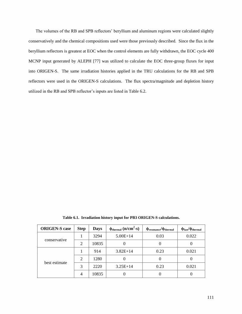
111
The volumes of the RB and SPB reflectors’ beryllium and aluminum regions were calculated slightly
conservatively and the chemical compositions used were those previously described. Since the flux in the
beryllium reflectors is greatest at EOC when the control elements are fully withdrawn, the EOC cycle 400
MCNP input generated by ALEPH [77] was utilized to calculate the EOC three-group fluxes for input
into ORIGEN-S. The same irradiation histories applied in the TRU calculations for the RB and SPB
reflectors were used in the ORIGEN-S calculations. The flux spectra/magnitude and depletion history
utilized in the RB and SPB reflector’s inputs are listed in Table 6.2.
Table 6.1. Irradiation history input for PB3 ORIGEN-S calculations.
ORIGEN-S case Step Days ϕthermal (n/cm2-s) ϕresonance/ϕthermal ϕfast/ϕthermal
conservative 1 3294 5.00E+14 0.03 0.022
2 10835 0 0 0
best estimate
1 914 3.82E+14 0.23 0.021
2 1280 0 0 0
3 2220 3.25E+14 0.23 0.021
4 10835 0 0 0

112
Table 6.2. Irradiation history input for RB and SPB ORIGEN-S calculations.
Reflector Region Step Days ϕthermal (n/cm2-s) ϕresonance/ϕthermal ϕfast/ϕthermal
RB 1 1200 8.823E+14 1.152 0.234
2 18262.5 0 0 0
SPB 1 2400 8.152E+14 0.498 0.058
2 18262.5 0 0 0
6.3 Beryllium Activation Results
The results for study number 1 are shown in Section 6.3.1. The results from study numbers 2 and 3
are shown in Section 6.3.2.
6.3.1 Startup Reactivity Effects Results
The beginning composition of the reflector regions was 100 % 9Be and equilibrium
6Li [0.90 g (1.29
μg/g Be): 0.67 g (4.47 μg/g Be) in RB and SPB, 0.23 g (0.42 μg/g Be) in PB] was achieved after
approximately 5 cycles (Figure 6.5). The results shown in Figure 6.5 reveal that the 3He inventory never
reaches equilibrium; it decreases during irradiation and increases during outages. Approximately 1.79
milligrams of 3He (2.55 ng/g Be) is produced in a typical cycle [1.40 mg (9.34 ng/g Be) in RB and SPB,
0.39 mg (0.71 ng/g Be) in PB]. Tritium and 4He were shown to increase in concentration at a rate of
approximately 0.38 grams (0.55 μg/g Be) [0.30 g (2.03 μg/g Be) in RB and SPB, 0.08 g (0.14 μg/g Be) in
PB] and 3.78 grams (5.39 μg/g Be) [3.00 g (20.03 μg/g Be) in RB and SPB, and 0.77 g (1.41 μg/g Be) in
PB] per typical cycle, respectively.
Effective multiplication factors were calculated for the reference case (BOC 21 keff) and the cases
corresponding to the multiple decay steps (BOC 22 keff). Since the 3He concentration increases as a
function of decay time between cycles, td, the keff values decreased as a function of td. All of the keff

113
values were inserted into a spreadsheet and the Δkeff/keff (%) values (reactivity effect of 3He as a function
of td) were calculated and converted into Δρ ($) (change in reactivity) by dividing by the delayed neutron
fraction (βeff = 0.00762). The Δρ’s were then converted into change in control element positions, ΔR’s,
using the conversion factor $3.10/inch; thereby determining the change in symmetrical critical control
element position associated with 3He worth with respect to the reference case. The actual differential rod
worth (DRW) is dependent upon the control element position, but a value of $3.10/inch corresponds to
―typical‖ startup positions (17.5 to 18 inches withdrawn).
Figure 6.5. Poison and gas buildup in the beryllium reflector resulting from neutron activation.
1.E-05
1.E-04
1.E-03
1.E-02
1.E-01
1.E+00
1.E+01
1.E+02
0 200 400 600 800 1000 1200 1400 1600 1800
Am
ou
nt
of
Isoto
pe
in R
efle
ctor
(gra
ms)
Days into Calculation (21 cycles + 730d decay)
Helium-4
Tritium
Lithium-6
Helium-3
20 cycles (25d irradiation + 25d
outage) + one 25d irradiation 730d outage

114
The purpose of this study is to determine the ―added‖ reactivity poisoning effect of 3He that builds in
following shutdown. Therefore, the Δρ curve was shifted such that the Δρ value at td = 0 is zero. The
curve based on a zero Δρ value at zero shutdown time is compared to the curve used in the current
ESCCEP calculation in Figure 6.6.
The proposed methodology for calculating the ΔR associated with 3He buildup is shown in Equation
6.10 where Td,C is the decay time on the reflector for the current cycle in days (outage time between the
shutdown of previous cycle and the startup of the current cycle) and Td,R is the decay time on the reflector
for the previous cycle in days. A second order polynomial based on the curve shown in Figure 6 was
used to convert from decay time to ΔR rather than a linear (first order) conversion, which is used in the
current methodology. If the current decay time is greater than the reference decay time the ΔR value is
positive and the control elements are withdrawn (due to a larger negative reactivity) and vice versa.
ΔR (inches) = 7.569x10⁻³
(Td,C - Td,R) – 3.477x10⁻⁶
[(Td,C)2 – (Td,R)
2]
Equation 6.10
ESCCEP calculations for HFIR cycles 383 – 421 [12] were utilized to compare the current and
proposed methodologies (Equation 6.10). For this study, it was assumed that uncertainty only exists in
the 3He worth (i.e., reactivity worth associated with fuel, cylinder/plate burnup, cylinder/plate
182Ta
worths, and etc. remained unchanged from the original calculations). The ESCCEPs calculated with both
the current and proposed methodologies were compared to the ASCCEPs and the differences are shown
in Figure 6.7.
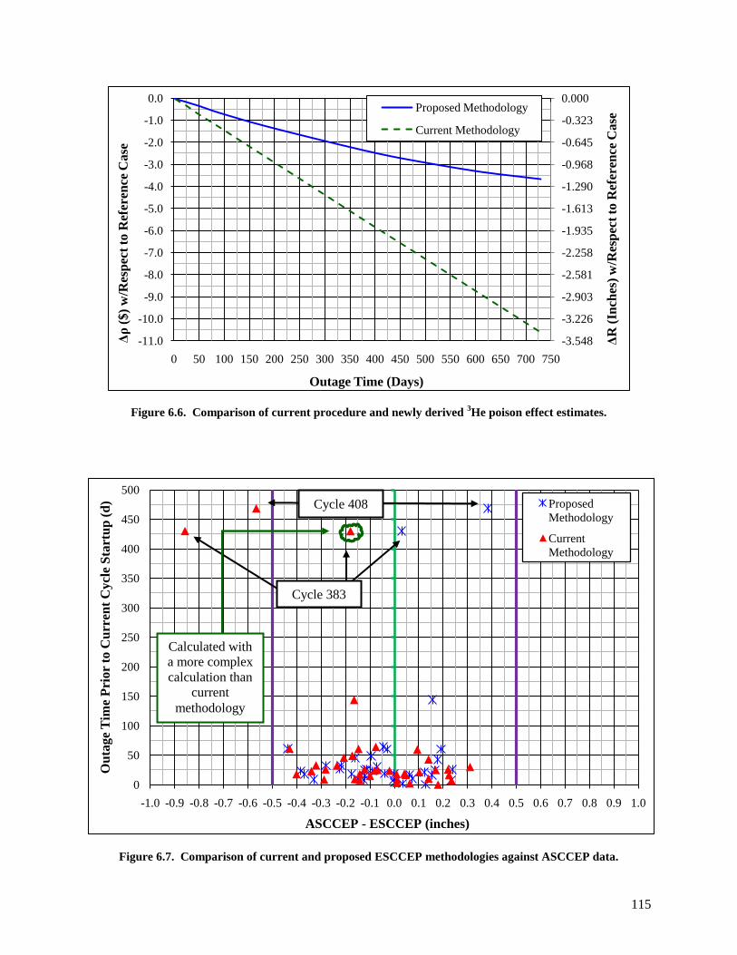
115
Figure 6.6. Comparison of current procedure and newly derived 3He poison effect estimates.
Figure 6.7. Comparison of current and proposed ESCCEP methodologies against ASCCEP data.
-3.548
-3.226
-2.903
-2.581
-2.258
-1.935
-1.613
-1.290
-0.968
-0.645
-0.323
0.000
-11.0
-10.0
-9.0
-8.0
-7.0
-6.0
-5.0
-4.0
-3.0
-2.0
-1.0
0.0
0 50 100 150 200 250 300 350 400 450 500 550 600 650 700 750
ΔR
(In
ches
) w
/Res
pec
t to
Ref
eren
ce C
ase
Δρ
($)
w/R
esp
ect
to R
efer
ence
Ca
se
Outage Time (Days)
Proposed Methodology
Current Methodology
0
50
100
150
200
250
300
350
400
450
500
-1.0 -0.9 -0.8 -0.7 -0.6 -0.5 -0.4 -0.3 -0.2 -0.1 0.0 0.1 0.2 0.3 0.4 0.5 0.6 0.7 0.8 0.9 1.0
Ou
tag
e T
ime
Pri
or
to C
urr
ent
Cycl
e S
tartu
p (
d)
ASCCEP - ESCCEP (inches)
Proposed
Methodology
Current
Methodology
Cycle 383
Cycle 408
Calculated with
a more complex
calculation than
current
methodology

116
On average, the proposed methodology better estimates the symmetrical critical control element
positions. The average absolute difference between the actual and estimated positions for the current and
proposed methodologies for the 39 cycles is 0.174 and 0.154 inches, respectively. The proposed
methodology better predicts the 3He effect for longer outages, but little difference is observed for shorter
outages. The lines in Figure 6.7 that extend at a delta of 0.5 inches were included because a difference of
~0.5 inches will cause the reactor to be shutdown and a technical evaluation to be performed to resolve
the discrepancy prior to startup. The difference of -0.56 inches calculated for cycle 408 using the current
methodology was the motivation of this study. A more involved calculation was used for cycle 383 (td =
430 days), which produced an ASCCEP – ESCCEP value of -0.180 inch. However, if the current
methodology would have been utilized, a difference of -0.858 inches would have been obtained. Thus,
the current methodology over-predicts the effects attributed to shutdown 3He and the proposed
methodology mitigates the over-prediction.
6.3.2 Nuclear Waste Classification Results
Permanent beryllium reflector number 3 along with representative RB and SPB reflectors were
depleted to determine whether they are discharged as- or following decay would become TRU waste. If
the beryllium reflectors are produced according to the current HFIR specification, discharged reflectors
would not be TRU waste, but the RB (reflector closest to the core) would become TRU waste
approximately 40 years after discharge. The current HFIR specification calls for the uranium content in
the beryllium reflectors to be less than or equal to 11 micrograms per gram of reflector (0.0011 wt. %),
but most previous reflectors have contained a greater quantity of uranium than the current specification
outlines. The initial uranium content in PB3 was 44 micrograms per gram of reflector (0.0044 wt. %).
Through calculations, it was concluded that with an initial uranium concentration of 0.0044 weight
percent, PB3 was discharged below the TRU waste threshold, but became TRU waste within three years
after being discharged. The RB and SPB reflectors were shown to be discharged as TRU waste if their

117
initial uranium content was greater than or equal to 0.0044 weight percent. The TRU waste inventories in
nCi per gram of waste as calculated with TRITON for the three reflector regions are shown in Figure 6.8.
The PB3 TRU waste inventories as calculated in TRITON and stand-alone ORIGEN-S are illustrated
in Figure 6.9. As observed in Figure 6.9, the two ORIGEN-S calculations are in similar agreement but
underestimate the total TRU inventory in comparison to the TRITON calculations. The two TRITON
calculations are in good agreement, but the results using a more accurate material composition and the
KENO-VI geometry predict a slightly greater TRU waste curie inventory. Input differences that caused
these small inventory discrepancies are discussed in Section 6.2.2. All four calculations support the
conclusion that PB3 currently exceeds the TRU waste limit. Note that PB3 was discharged in October of
2000.
Figure 6.8. TRU waste inventory in beryllium reflector regions following discharge.
0
50
100
150
200
250
300
350
400
0 5 10 15 20 25 30 35 40 45 50
TR
U W
ast
e R
ad
ioacti
vit
y (
nC
i/g w
ast
e)
Years After Discharge
RB (0.0044wt%U) SPB (0.0044wt%U) PB3 (0.0044wt%U)
RB (0.0011wt%U) SPB (0.0011wt%U) PB3 (0.0011wt%U)
TRU Threshold

118
Figure 6.9. TRU waste inventory in PB3 following discharge.
The June 2010 radionuclide curie levels of the major curie contributing nuclides in PB3 and as
calculated in TRITON and ORIGEN-S are shown in Figure 6.10. The bar plot shows that the ORIGEN-S
calculations estimated larger inventories of light elements in comparison to TRITON, and TRITON
calculated larger inventories of fission products in comparison to ORIGEN-S. The total PB3 radioactivity
as calculated in TRITON, a best estimate ORIGEN-S calculation, and a conservative ORIGEN-S
calculation as of June 2010 are 68 kCi, 101 kCi, and 161 kCi, respectively. Tritium, a beta emitter,
contributes approximately 99 % of the total radioactivity (Ci) while 60
Co and 137
Cs (sources leading to
high energy gamma rays) contribute approximately 0.35 % and 0.01 % - 0.04 %, respectively.
50
75
100
125
150
175
200
225
0 3 6 9 12 15 18 21 24 27 30
TR
U W
ast
e R
ad
ioact
ivit
y (
nC
i/g w
ast
e)
Years After PB3 Discharged
TRITON (KENO-VI)
TRITON (KENO V.a)
ORIGEN-S (Conservative)
ORIGEN-S (BestEstimate)

119
Figure 6.10. June 2010 radionuclide curie levels in PB3 as calculated in TRITON (left), ORIGEN-S best
estimate (middle), and ORIGEN-S conservative (right).
The primary radionuclides in PB3 following discharge are shown in Table 6.3. The table lists
nuclides present in quantities greater than 1 Ci at 9.67 years after discharge (i.e., June 2010) sorted in
descending order. The values for the 15 nuclides in Table 3 are the largest values calculated in either
TRITON or stand-alone ORIGEN-S. The radioactivity listed for 137
Cs, 137m
Ba, 90
Y, 90
Sr, and 241
Pu were
produced by the TRITON calculation and the rest were calculated by ORIGEN-S. After comparing all of
these values to the hazard category thresholds [91] using the sum-of-the-fractions approach, it is
concluded that PB3 can be classified as nuclear hazard category 3.
1.E-01
1.E+00
1.E+01
1.E+02
1.E+03
1.E+04
1.E+05
1.E+06
tota
l
h3
fe55
co6
0
c14
ni6
3
cs137
ba1
37m
be1
0
cm244
y90
sr90
pu241
cs134
Ra
dio
acti
vit
y (
Cu
ries
)
Isotope
TRITON
ORIGEN-S (best estimate)
ORIGEN-S (conservative)
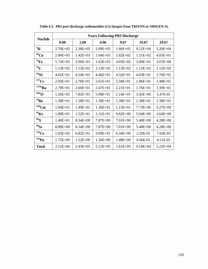
120
Table 6.3. PB3 post-discharge radionuclides (Ci) (largest from TRITON or ORIGEN-S).
Nuclide Years Following PB3 Discharge
0.00 2.60 4.96 9.67 19.67 29.67
3H 2.76E+05 2.38E+05 2.09E+05 1.60E+05 9.12E+04 5.20E+04
60Co 2.00E+03 1.42E+03 1.04E+03 5.62E+02 1.51E+02 4.05E+01
55Fe 5.73E+03 2.96E+03 1.63E+03 4.93E+02 3.89E+01 3.07E+00
14C 1.13E+02 1.13E+02 1.13E+02 1.13E+02 1.12E+02 1.12E+02
63Ni 4.62E+01 4.54E+01 4.46E+01 4.32E+01 4.03E+01 3.76E+01
137Cs 2.93E+01 2.76E+01 2.61E+01 2.34E+01 1.86E+01 1.48E+01
137mBa 2.79E+01 2.60E+01 2.47E+01 2.21E+01 1.76E+01 1.39E+01
204Tl 1.26E+02 7.82E+01 5.08E+01 2.14E+01 3.42E+00 5.47E-01
10Be 1.38E+01 1.38E+01 1.38E+01 1.38E+01 1.38E+01 1.38E+01
244Cm 1.64E+01 1.49E+01 1.36E+01 1.13E+01 7.73E+00 5.27E+00
85Kr 1.80E+01 1.52E+01 1.31E+01 9.62E+00 5.04E+00 2.64E+00
90Y 1.40E+01 8.34E+00 7.87E+00 7.01E+00 5.48E+00 4.28E+00
90Sr 8.89E+00 8.34E+00 7.87E+00 7.01E+00 5.48E+00 4.28E+00
134Cs 1.63E+02 6.82E+01 3.09E+01 6.34E+00 2.20E-01 7.63E-03
241Pu 1.72E+00 1.52E+00 1.36E+00 1.08E+00 6.66E-01 4.11E-01
Total 3.12E+06 2.43E+05 2.12E+05 1.61E+05 9.16E+04 5.22E+04
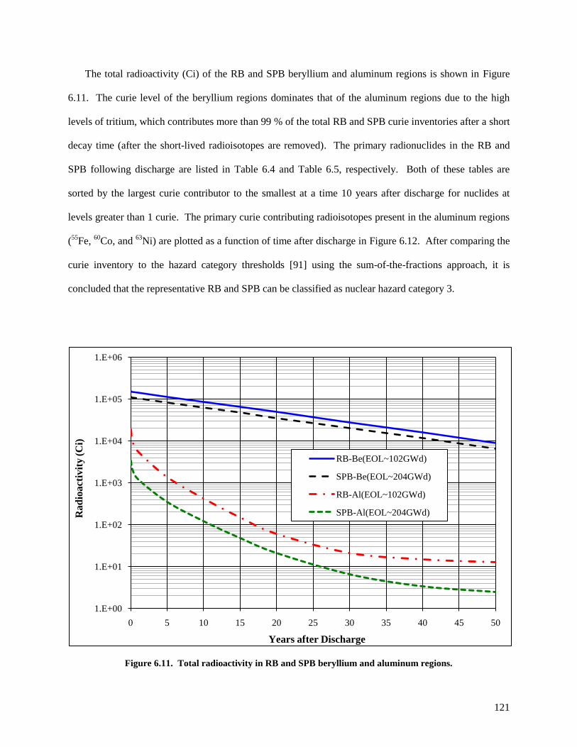
121
The total radioactivity (Ci) of the RB and SPB beryllium and aluminum regions is shown in Figure
6.11. The curie level of the beryllium regions dominates that of the aluminum regions due to the high
levels of tritium, which contributes more than 99 % of the total RB and SPB curie inventories after a short
decay time (after the short-lived radioisotopes are removed). The primary radionuclides in the RB and
SPB following discharge are listed in Table 6.4 and Table 6.5, respectively. Both of these tables are
sorted by the largest curie contributor to the smallest at a time 10 years after discharge for nuclides at
levels greater than 1 curie. The primary curie contributing radioisotopes present in the aluminum regions
(55
Fe, 60
Co, and 63
Ni) are plotted as a function of time after discharge in Figure 6.12. After comparing the
curie inventory to the hazard category thresholds [91] using the sum-of-the-fractions approach, it is
concluded that the representative RB and SPB can be classified as nuclear hazard category 3.
Figure 6.11. Total radioactivity in RB and SPB beryllium and aluminum regions.
1.E+00
1.E+01
1.E+02
1.E+03
1.E+04
1.E+05
1.E+06
0 5 10 15 20 25 30 35 40 45 50
Ra
dio
acti
vit
y (
Ci)
Years after Discharge
RB-Be(EOL~102GWd)
SPB-Be(EOL~204GWd)
RB-Al(EOL~102GWd)
SPB-Al(EOL~204GWd)
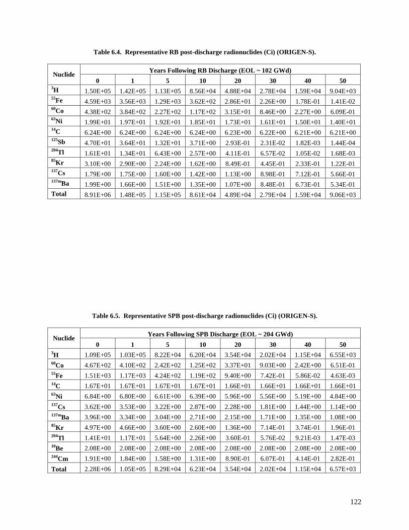
122
Table 6.4. Representative RB post-discharge radionuclides (Ci) (ORIGEN-S).
Nuclide Years Following RB Discharge (EOL ~ 102 GWd)
0 1 5 10 20 30 40 50 3H 1.50E+05 1.42E+05 1.13E+05 8.56E+04 4.88E+04 2.78E+04 1.59E+04 9.04E+03
55Fe 4.59E+03 3.56E+03 1.29E+03 3.62E+02 2.86E+01 2.26E+00 1.78E-01 1.41E-02
60Co 4.38E+02 3.84E+02 2.27E+02 1.17E+02 3.15E+01 8.46E+00 2.27E+00 6.09E-01
63Ni 1.99E+01 1.97E+01 1.92E+01 1.85E+01 1.73E+01 1.61E+01 1.50E+01 1.40E+01
14C 6.24E+00 6.24E+00 6.24E+00 6.24E+00 6.23E+00 6.22E+00 6.21E+00 6.21E+00
125Sb 4.70E+01 3.64E+01 1.32E+01 3.71E+00 2.93E-01 2.31E-02 1.82E-03 1.44E-04
204Tl 1.61E+01 1.34E+01 6.43E+00 2.57E+00 4.11E-01 6.57E-02 1.05E-02 1.68E-03
85Kr 3.10E+00 2.90E+00 2.24E+00 1.62E+00 8.49E-01 4.45E-01 2.33E-01 1.22E-01
137Cs 1.79E+00 1.75E+00 1.60E+00 1.42E+00 1.13E+00 8.98E-01 7.12E-01 5.66E-01
137mBa 1.99E+00 1.66E+00 1.51E+00 1.35E+00 1.07E+00 8.48E-01 6.73E-01 5.34E-01
Total 8.91E+06 1.48E+05 1.15E+05 8.61E+04 4.89E+04 2.79E+04 1.59E+04 9.06E+03
Table 6.5. Representative SPB post-discharge radionuclides (Ci) (ORIGEN-S).
Nuclide Years Following SPB Discharge (EOL ~ 204 GWd)
0 1 5 10 20 30 40 50 3H 1.09E+05 1.03E+05 8.22E+04 6.20E+04 3.54E+04 2.02E+04 1.15E+04 6.55E+03
60Co 4.67E+02 4.10E+02 2.42E+02 1.25E+02 3.37E+01 9.03E+00 2.42E+00 6.51E-01
55Fe 1.51E+03 1.17E+03 4.24E+02 1.19E+02 9.40E+00 7.42E-01 5.86E-02 4.63E-03
14C 1.67E+01 1.67E+01 1.67E+01 1.67E+01 1.66E+01 1.66E+01 1.66E+01 1.66E+01
63Ni 6.84E+00 6.80E+00 6.61E+00 6.39E+00 5.96E+00 5.56E+00 5.19E+00 4.84E+00
137Cs 3.62E+00 3.53E+00 3.22E+00 2.87E+00 2.28E+00 1.81E+00 1.44E+00 1.14E+00
137mBa 3.96E+00 3.34E+00 3.04E+00 2.71E+00 2.15E+00 1.71E+00 1.35E+00 1.08E+00
85Kr 4.97E+00 4.66E+00 3.60E+00 2.60E+00 1.36E+00 7.14E-01 3.74E-01 1.96E-01
204Tl 1.41E+01 1.17E+01 5.64E+00 2.26E+00 3.60E-01 5.76E-02 9.21E-03 1.47E-03
10Be 2.08E+00 2.08E+00 2.08E+00 2.08E+00 2.08E+00 2.08E+00 2.08E+00 2.08E+00
244Cm 1.91E+00 1.84E+00 1.58E+00 1.31E+00 8.90E-01 6.07E-01 4.14E-01 2.82E-01
Total 2.28E+06 1.05E+05 8.29E+04 6.23E+04 3.54E+04 2.02E+04 1.15E+04 6.57E+03

123
Figure 6.12. Major RB and SPB aluminum region radionuclides.
6.4 Beryllium Activation Summary
Helium-3 is produced and depleted during operation (neutron flux environment) and is produced
during an outage (no neutron flux environment) due to the radioactive decay of tritium. A newly-derived
correlation was developed and shown to improve the accuracy of predicting the symmetrical critical
control element positions following long periods of down time between cycles. The newly-derived
methodology is currently being incorporated in the HFIR Estimated Symmetrical Critical Control
Element Position procedure. The explanation for the observed inadequacy of the current procedure for
predicting the poisoning effect following long shutdowns (several months) is due to the buildup of 3He in
the reflector as a function of decay time not corresponding to a linear decrease in reactivity. The current
procedure for estimating poisoning effects had assumed a linear relationship and an operating power of
1.E-03
1.E-02
1.E-01
1.E+00
1.E+01
1.E+02
1.E+03
1.E+04
0 5 10 15 20 25 30 35 40 45 50
Nu
clid
e A
ctiv
ity
(C
i)
Years after Discharge
RB: Fe-55 in Al SPB: Fe-55 in Al
RB: Co-60 in Al SPB: Co-60 in Al
RB: Ni-63 in Al SPB: Ni-63 in Al

124
100 MWth. The results derived serve to validate the SCALE system and associated cross section libraries
for predicting the in-growth of nuclides during irradiation of beryllium.
The results leading to the new reflector reactivity prediction methodology also provided insight into
the production rate of other significant nuclides in the beryllium reflector regions. 6Li was shown to reach
an equilibrium concentration of approximately 1.29 μg/g Be after four to five full power cycles. Helium-
3 was shown to never achieve equilibrium and is produced at a rate of approximately 2.55 ng/g Be per
typical cycle. Tritium, a radiolytic gas, is produced at a rate of approximately 0.55 μg/g Be per typical
cycle. Tritium is the major curie contributor in spent reflectors and although it is tightly bound in the
beryllium lattice, it can be released if the beryllium begins to corrode [83]. Helium-4 is produced at a rate
of approximately 5.39 μg/g Be per typical cycle and is a gas that causes the beryllium reflector regions to
swell and crack, and therefore, dictates the life span of the reflector regions.
If the reflector regions are manufactured to the current HFIR specification of less than or equal to 11
micrograms of uranium per gram of reflector, then the reflectors would be discharged below the
transuranic waste threshold with the possibility of the RB exceeding the threshold after approximately 40
years of decay. If the initial uranium concentration is greater than or equal to 44 micrograms per gram of
reflector, then PB3 became transuranic waste approximately two to three years after being discharged and
representative RB and SPB reflectors are discharged as transuranic waste. The maximum initial uranium
concentration that could be accommodated without exceeding the transuranic waste threshold was not
determined, but it appears to be close to the 11 microgram per gram limit.
Therefore, the amount of uranium impurity in the fresh beryllium reflectors is a concern because the
initial amount of uranium dictates whether or not the reflectors become transuranic waste. Classification
of the reflectors as transuranic waste also categorizes them as ―waste with no identified path to disposal‖
since the isotopic content exceeds the acceptance criteria for the Nevada Test Site [90] and non-defense
transuranic waste is not currently accepted at the Waste Isolation Pilot Plant in New Mexico [95]. In
addition to the transuranic waste determination, other factors such as the 14
C concentrations being greater
125
than the Class C upper activity limit of 80 Ci/m3 in activated metal [96] contribute to the designation of
no path to disposal.
The total curie inventory of PB3 as of June 2010 and as calculated in TRITON is approximately 67.6
kCi, and 21 different radionuclides with curie levels greater than 0.1 Ci contribute to this radioactivity.
The predominant radionuclide is tritium at 66.8 kCi (~6.91 grams). The predominant gamma emitter is
60Co at 221 Ci (~0.20 grams). Other contributing nuclides include:
55Fe,
14C, and
63Ni at 386, 89, and 42
Ci, respectively. After 10 years of decay, the total radioactivity of a representative RB and SPB reflector
as calculated in stand-alone ORIGEN-S is 861 kCi and 623 kCi, respectively, and over 99 % of the
radioactivity is contributed by tritium. The major gamma emitter, 60
Co, is present at curie levels of 117
and 125 Ci in the RB and SPB, respectively, after 10 years of decay.
According to the radionuclide threshold limits defined in DOE-STD-1027 [91], PB3 is currently
nuclear hazard category 3. Representative RB and SPB reflectors were also shown to be hazard category
3. The nuclear hazard category and the specific isotopic inventories can be used to determine whether the
reflectors fit within the authorized limits specified in the safety basis for the proposed temporary storage
location. If that is found to be the case, the hazard category and isotopic inventories will be used to
develop a transportation safety document for moving the reflectors from the spent fuel pool to the storage
location.
The stand-alone ORIGEN-S calculations were shown to over-predict the tritium inventory and under-
predict the transuranic waste inventory in comparison to the TRITON calculations. It is therefore shown
that more details need to be inserted into stand-alone ORIGEN-S calculations in order to properly predict
the total nuclide inventory in the beryllium reflector regions. The best estimate ORIGEN-S calculations
utilized the cycle-averaged thermal, resonance, and fast neutron fluxes in the permanent beryllium
reflector as calculated with benchmarked MCNP calculations. Thus, it is shown here that modeling the
permanent reflector as a point is not sufficient for this application, and therefore, the reflectors must be
depleted via a radially varying neutron flux.
126
7 Post-Irradiation Curium Target Rod Inventory
In this chapter, the post-irradiation compositions of curium target rods that were irradiated for several
cycles in the flux-trap target region (FTT) of HFIR were calculated and compared to dissolver solution
measurements. This study was performed in order to validate the SCALE/KENO model of HFIR and the
ENDF/B-VII neutron cross section libraries for predicting the composition, specifically the amount of
californium-252 and berkelium-249, of target rods following irradiation.
HFIR was originally designed to produce transplutonium isotopes such as 252
Cf. The FTT region
contains 37 experiment sites and is located at the center of the reactor. At full power (85 MWth), a peak
thermal neutron flux of about 2.2x10¹⁵
neutrons/cm2-s exists in the flux trap, which is an excellent neutron
environment for producing 252
Cf and other transplutonium isotopes. Following the irradiation of target
rods in HFIR, the Radiochemical Engineering Development Center (REDC) processes the targets for the
separation, recovery, and purification of the heavy elements (Bk, Cf, Es, and Fm). The dissolver solution
processing method includes chemical dissolution of the targets followed by a series of solvent extraction,
ion exchange, and precipitation steps to separate and purify the heavy elements.
A summary of the flux trap loading for all cycles up to cycle 425 is shown in Figure 7.1. This figure
shows the types of targets loaded into the interior flux trap positions (total of 31 interior positions) and the
percentage of the interior flux trap positions that they occupied. Aluminum target rods are utilized in the
flux trap when experimental targets are not being irradiated to satisfy coolant flow restrictions. The target
feedstock was originally 239
Pu and 242
Pu, but then changed to curium, which was produced from the
Savannah River reactors. If the feedstock is plutonium, only 0.3 % and 3.0 % of the initial 239
Pu and 242
Pu
atoms are transmuted into 252
Cf, respectively. However, when starting with curium as feed, 3.0 %, 20 %,
and 38 % of the initial 244
Cm, 246
Cm, and 248
Cm atoms are transmuted into 252
Cf.

127
Figure 7.1. Flux trap loading summary (407 – 418 are boxed in and are the focus of this study).
0%
20
%4
0%
60
%8
0%
10
0%
1 30 58 88 118a 147 177 206 236 264 294 324 354 384 411
Per
cen
tag
e o
f In
teri
or
Ta
rget
s
HFIR Fuel Cycle Number
Other
Al
Cf
Cm
Pu
U235

128
7.1 Curium Target Information
Seven transuranic target rods were removed from the FTT following the shutdown of cycle 418
(December 5, 2008) and analyzed via dissolver solution on March 21, 2009 [97]. Target rods S28, S30,
S31, S32, S33, and S34 were irradiated during HFIR cycles 408 – 418 (21643 MWd) [98] while target
rod S27 was irradiated during cycles 407 - 418 (23642 MWd) [99]. Target S27 was irradiated for 23.51
days followed by a 485 day decay period (cycle 407). Targets S28, S30, S31, S32, S33, and S34 were
inserted into the FTT at the startup of cycle 408 (with S27 still loaded). A summary of the HFIR fuel
cycles 407 – 418 is listed in Table 7.1 and shows the irradiation and decay history for these targets. The
experiment configuration of targets within the FTT is shown in Figure 7.2. Targets S27, S28, S30, S31,
S32, S33, and S34 were irradiated in target locations C4, C1, F5, C5, E5, E4, and C3, respectively.
Initially, the target rods contained between 6.47 and 7.68 grams of actinides and were composed of
either 31 or 35 pellets. Each pellet was initially composed of approximately 51 wt. % 246
Cm, 23 wt. %
244Cm, 11 wt. %
248Cm, 7.3 wt. %
243Am, 3.7 wt. %
240Pu, 2.2 wt. %
241Am, 1.5 wt. %
247Cm, as well as
trace amounts of other Pu, Cm, Am, Bk, and Cf isotopes, [98] and [99]. The initial actinide loading for
the seven targets are listed in Table 7.2.

129
Table 7.1. Irradiation history of target rods.
Cycle # Cycle Startup Cycle Shutdown
407 12/21/2005 8:51 1/13/2006 21:08
408a 5/13/2007 21:58 5/14/2007 20:21
408b 5/15/2007 21:24 6/9/2007 15:30
409 6/27/2007 8:05 7/20/2007 16:00
410a 8/15/2007 8:09 9/3/2007 12:00
410b 9/26/2007 7:32 9/26/2007 13:10
410c 9/28/2007 4:34 10/2/2007 13:42
411 11/14/2007 7:31 12/8/2007 0:43
412 12/18/2007 10:22 1/11/2008 2:00
413 2/6/2008 9:47 3/1/2008 9:00
414 3/26/2008 12:10 4/19/2008 14:14
415a 6/7/2008 21:35 6/21/2008 21:06
415b 6/26/2008 8:18 6/30/2008 5:25
416 7/16/2008 8:02 8/6/2008 10:46
417 9/24/2008 7:46 10/18/2008 6:50
418 11/12/2008 8:01 12/5/2008 19:30
Figure 7.2. Illustration of the flux trap target positions.
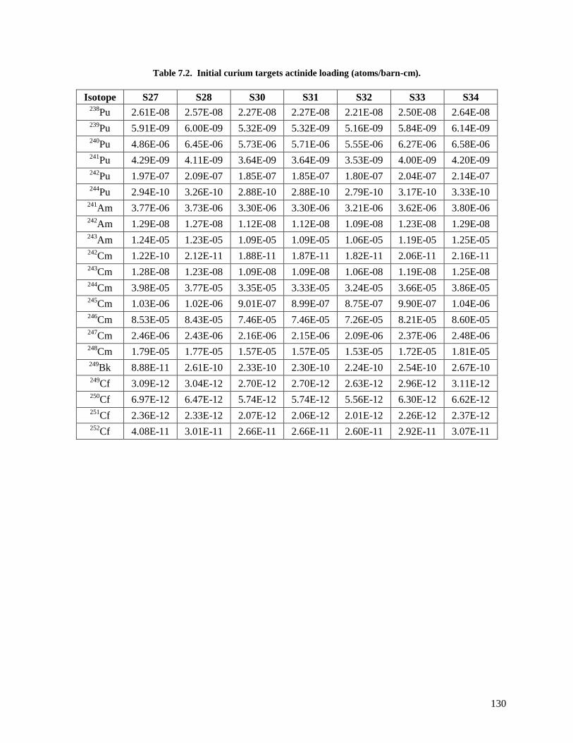
130
Table 7.2. Initial curium targets actinide loading (atoms/barn-cm).
Isotope S27 S28 S30 S31 S32 S33 S34 238
Pu 2.61E-08 2.57E-08 2.27E-08 2.27E-08 2.21E-08 2.50E-08 2.64E-08 239
Pu 5.91E-09 6.00E-09 5.32E-09 5.32E-09 5.16E-09 5.84E-09 6.14E-09 240
Pu 4.86E-06 6.45E-06 5.73E-06 5.71E-06 5.55E-06 6.27E-06 6.58E-06 241
Pu 4.29E-09 4.11E-09 3.64E-09 3.64E-09 3.53E-09 4.00E-09 4.20E-09 242
Pu 1.97E-07 2.09E-07 1.85E-07 1.85E-07 1.80E-07 2.04E-07 2.14E-07 244
Pu 2.94E-10 3.26E-10 2.88E-10 2.88E-10 2.79E-10 3.17E-10 3.33E-10 241
Am 3.77E-06 3.73E-06 3.30E-06 3.30E-06 3.21E-06 3.62E-06 3.80E-06 242
Am 1.29E-08 1.27E-08 1.12E-08 1.12E-08 1.09E-08 1.23E-08 1.29E-08 243
Am 1.24E-05 1.23E-05 1.09E-05 1.09E-05 1.06E-05 1.19E-05 1.25E-05 242
Cm 1.22E-10 2.12E-11 1.88E-11 1.87E-11 1.82E-11 2.06E-11 2.16E-11 243
Cm 1.28E-08 1.23E-08 1.09E-08 1.09E-08 1.06E-08 1.19E-08 1.25E-08 244
Cm 3.98E-05 3.77E-05 3.35E-05 3.33E-05 3.24E-05 3.66E-05 3.86E-05 245
Cm 1.03E-06 1.02E-06 9.01E-07 8.99E-07 8.75E-07 9.90E-07 1.04E-06 246
Cm 8.53E-05 8.43E-05 7.46E-05 7.46E-05 7.26E-05 8.21E-05 8.60E-05 247
Cm 2.46E-06 2.43E-06 2.16E-06 2.15E-06 2.09E-06 2.37E-06 2.48E-06 248
Cm 1.79E-05 1.77E-05 1.57E-05 1.57E-05 1.53E-05 1.72E-05 1.81E-05 249
Bk 8.88E-11 2.61E-10 2.33E-10 2.30E-10 2.24E-10 2.54E-10 2.67E-10 249
Cf 3.09E-12 3.04E-12 2.70E-12 2.70E-12 2.63E-12 2.96E-12 3.11E-12 250
Cf 6.97E-12 6.47E-12 5.74E-12 5.74E-12 5.56E-12 6.30E-12 6.62E-12 251
Cf 2.36E-12 2.33E-12 2.07E-12 2.06E-12 2.01E-12 2.26E-12 2.37E-12 252
Cf 4.08E-11 3.01E-11 2.66E-11 2.66E-11 2.60E-11 2.92E-11 3.07E-11

131
7.2 Computational Methodology
Version 6 of the SCALE package and the 238-group ENDF/B-VII nuclear data library [56] were
utilized in this study. The 3-D TRITON depletion sequence in SCALE, which couples the Monte Carlo
transport code KENO V.a and the depletion and decay code ORIGEN-S, was employed for burnup
simulations. The flux trap target region in the SCALE/KENO model discussed in Chapter 6 was
modified as needed to be applicable to this analysis. The target rods, which are 50.8 cm in length and
0.835 cm in radius, were modeled by homogenizing the Al-actinide-oxide pellets, Al-6061 pellet clad, Al-
6061 outer shroud, Al target tube, and coolant (water) rather than modeling each separately. The initial
actinide loading of the seven target rods are listed in Table 7.2. Each of the target rod’s materials was
simulated as individual depletion mixtures such that each homogenized target rod was depleted
individually and by different fluxes. An isometric view of the KENO model used for this analysis is
illustrated in Figure 6.3. The flux trap target region of the KENO model as developed specifically for this
analysis is shown in Figure 7.3.
The thermal and non-thermal fluxes in the FTT region are almost identical for a clean and depleted
core because the control elements are external to the annular reactor core. Thus, the neutron flux level
remains effectively constant in the flux trap as a function of time during full power irradiation. Fuel was
therefore not depleted and control element withdrawal was not simulated during the irradiation periods.
The thermal and total flux fields as calculated in KENO are compared to those calculated in MCNP at
BOC and EOC conditions in Figure 7.4. The flux trap loading in the MCNP model has no transuranic
targets loaded so the fluxes will differ slightly. Curium targets absorb neutrons, and thus, it is expected
that the flux in the flux trap and fuel regions be slightly lower for the KENO calculation. The irradiation
and decay history described in Table 7.1 was defined in the TRITON input. Each cycle was modeled to
include irradiation and outage periods, and reactivity was controlled (critical condition maintained) by
inserting poison into the control element region.
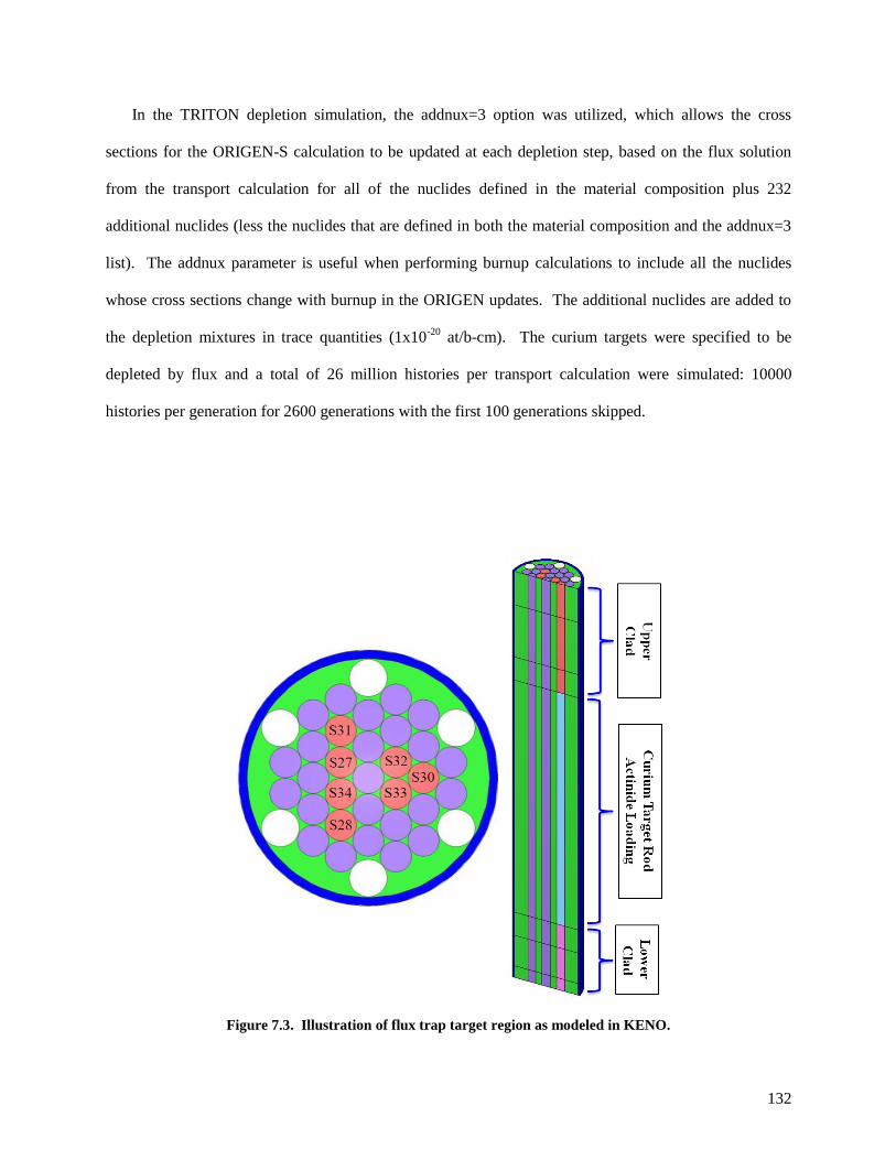
132
In the TRITON depletion simulation, the addnux=3 option was utilized, which allows the cross
sections for the ORIGEN-S calculation to be updated at each depletion step, based on the flux solution
from the transport calculation for all of the nuclides defined in the material composition plus 232
additional nuclides (less the nuclides that are defined in both the material composition and the addnux=3
list). The addnux parameter is useful when performing burnup calculations to include all the nuclides
whose cross sections change with burnup in the ORIGEN updates. The additional nuclides are added to
the depletion mixtures in trace quantities (1x10-20
at/b-cm). The curium targets were specified to be
depleted by flux and a total of 26 million histories per transport calculation were simulated: 10000
histories per generation for 2600 generations with the first 100 generations skipped.
Figure 7.3. Illustration of flux trap target region as modeled in KENO.

133
Figure 7.4. KENO and validated MCNP axially averaged flux comparison.
7.3 Curium Target Results
The twenty most abundant transuranic isotopes calculated following the shutdown of cycle 418 are
listed in Table 7.3. The inventory listed is the sum of all seven target rods. Following the shutdown of
cycle 418, the targets were decayed for 106 days to the date corresponding to the day the dissolver
solution measurements were performed. After the 106 day decay, a total of 248.65 mg of 252
Cf and 33.40
mg of 249
Bk were calculated for the seven target rods. The corresponding values from the dissolver
solution measurements were 250 and 31 mg of 252
Cf and 249
Bk, respectively [97]. The calculated-to-
experimental (C/E) ratios for 252
Cf and 249
Bk are 0.995 and 1.077, respectively. Experimental
uncertainties and other nuclide dissolver solution measurements are desired for comparison purposes, but
were not provided. The time-dependent 252
Cf and 249
Bk inventories are shown in Figure 7.5.
0.0E+00
5.0E+14
1.0E+15
1.5E+15
2.0E+15
2.5E+15
3.0E+15
3.5E+15
4.0E+15
0 5 10 15 20 25 30 35 40 45 50 55
Axia
lly
Av
era
ged
Neu
tro
n F
lux
(n
/cm
2-s
)
Distance from core centerline (cm)
KENO VI (0-20MeV)
KENO VI (0-3eV)
MCNP BOC (0-20MeV)
MCNP BOC (0-3eV)
MCNP EOC (0-20MeV)
MCNP EOC (0-3eV)

134
Table 7.3. Calculated end-of-life transuranic nuclide inventory in curium targets.
Isotope Grams Isotope Grams 238
Pu 0.00219 246
Cm 21.45000 239
Pu 0.00119 247
Cm 0.52730 240
Pu 0.00751 248
Cm 4.83900 241
Pu 0.00417 249
Bk 0.03923 242
Pu 0.10760 250
Bk 0.00151 244
Pu 0.00242 250
Cf 0.02579 243
Am 0.08786 251
Cf 0.00684 242
Cm 0.02145 252
Cf 0.26770 244
Cm 4.26500 253
Cf 0.00281 245
Cm 0.07038 254
Cf 0.00575
Figure 7.5. Calculated time-dependent 252
Cf and 249
Bk inventories.
0
5
10
15
20
25
30
35
40
45
50
0
30
60
90
120
150
180
210
240
270
300
0 100 200 300 400 500 600 700 800
24
9B
k in
7
T
arg
ets
(m
illi
gra
ms)
25
2C
f i
n 7
T
arg
ets
(m
illi
gra
ms)
Time From BOC 408 (days)
Cf252
Bk249
33.4 mg
248.7 mg
3/21/2009

135
7.4 Curium Target Summary
Post-irradiation curium target rod nuclide inventories were calculated for seven targets that were
removed from the flux trap in December of 2008. Dissolver solution measurements for 252
Cf and 249
Bk
were compared to the calculations and C/E ratios of 0.995 and 1.077 were calculated, respectively. The
differences between the calculated and measured post-irradiation curium target rod 252
Cf and 249
Bk
inventory are small and thus, the SCALE code/model with the 238-group ENDF/B-VII data library has
proven to be able to accurately calculate the burnup dependent inventories for these nuclides within the
target rods. The studies provide validation that the SCALE/TRITON module and ENDF/B-VII cross
section data can accurately calculate the homogenized cross sections and neutron fluxes in curium targets
located in the flux trap region of HFIR.
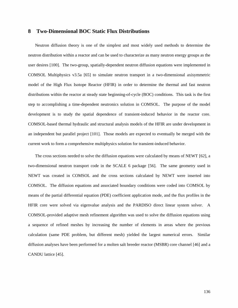
136
8 Two-Dimensional BOC Static Flux Distributions
Neutron diffusion theory is one of the simplest and most widely used methods to determine the
neutron distribution within a reactor and can be used to characterize as many neutron energy groups as the
user desires [100]. The two-group, spatially-dependent neutron diffusion equations were implemented in
COMSOL Multiphysics v3.5a [65] to simulate neutron transport in a two-dimensional axisymmetric
model of the High Flux Isotope Reactor (HFIR) in order to determine the thermal and fast neutron
distributions within the reactor at steady state beginning-of-cycle (BOC) conditions. This task is the first
step to accomplishing a time-dependent neutronics solution in COMSOL. The purpose of the model
development is to study the spatial dependence of transient-induced behavior in the reactor core.
COMSOL-based thermal hydraulic and structural analysis models of the HFIR are under development in
an independent but parallel project [101]. Those models are expected to eventually be merged with the
current work to form a comprehensive multiphysics solution for transient-induced behavior.
The cross sections needed to solve the diffusion equations were calculated by means of NEWT [62], a
two-dimensional neutron transport code in the SCALE 6 package [56]. The same geometry used in
NEWT was created in COMSOL and the cross sections calculated by NEWT were inserted into
COMSOL. The diffusion equations and associated boundary conditions were coded into COMSOL by
means of the partial differential equation (PDE) coefficient application mode, and the flux profiles in the
HFIR core were solved via eigenvalue analysis and the PARDISO direct linear system solver. A
COMSOL-provided adaptive mesh refinement algorithm was used to solve the diffusion equations using
a sequence of refined meshes by increasing the number of elements in areas where the previous
calculation (same PDE problem, but different mesh) yielded the largest numerical errors. Similar
diffusion analyses have been performed for a molten salt breeder reactor (MSBR) core channel [46] and a
CANDU lattice [45].
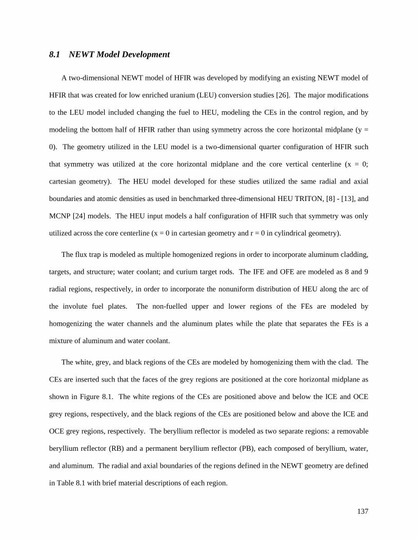
137
8.1 NEWT Model Development
A two-dimensional NEWT model of HFIR was developed by modifying an existing NEWT model of
HFIR that was created for low enriched uranium (LEU) conversion studies [26]. The major modifications
to the LEU model included changing the fuel to HEU, modeling the CEs in the control region, and by
modeling the bottom half of HFIR rather than using symmetry across the core horizontal midplane (y =
0). The geometry utilized in the LEU model is a two-dimensional quarter configuration of HFIR such
that symmetry was utilized at the core horizontal midplane and the core vertical centerline (x = 0;
cartesian geometry). The HEU model developed for these studies utilized the same radial and axial
boundaries and atomic densities as used in benchmarked three-dimensional HEU TRITON, [8] - [13], and
MCNP [24] models. The HEU input models a half configuration of HFIR such that symmetry was only
utilized across the core centerline (x = 0 in cartesian geometry and r = 0 in cylindrical geometry).
The flux trap is modeled as multiple homogenized regions in order to incorporate aluminum cladding,
targets, and structure; water coolant; and curium target rods. The IFE and OFE are modeled as 8 and 9
radial regions, respectively, in order to incorporate the nonuniform distribution of HEU along the arc of
the involute fuel plates. The non-fuelled upper and lower regions of the FEs are modeled by
homogenizing the water channels and the aluminum plates while the plate that separates the FEs is a
mixture of aluminum and water coolant.
The white, grey, and black regions of the CEs are modeled by homogenizing them with the clad. The
CEs are inserted such that the faces of the grey regions are positioned at the core horizontal midplane as
shown in Figure 8.1. The white regions of the CEs are positioned above and below the ICE and OCE
grey regions, respectively, and the black regions of the CEs are positioned below and above the ICE and
OCE grey regions, respectively. The beryllium reflector is modeled as two separate regions: a removable
beryllium reflector (RB) and a permanent beryllium reflector (PB), each composed of beryllium, water,
and aluminum. The radial and axial boundaries of the regions defined in the NEWT geometry are defined
in Table 8.1 with brief material descriptions of each region.
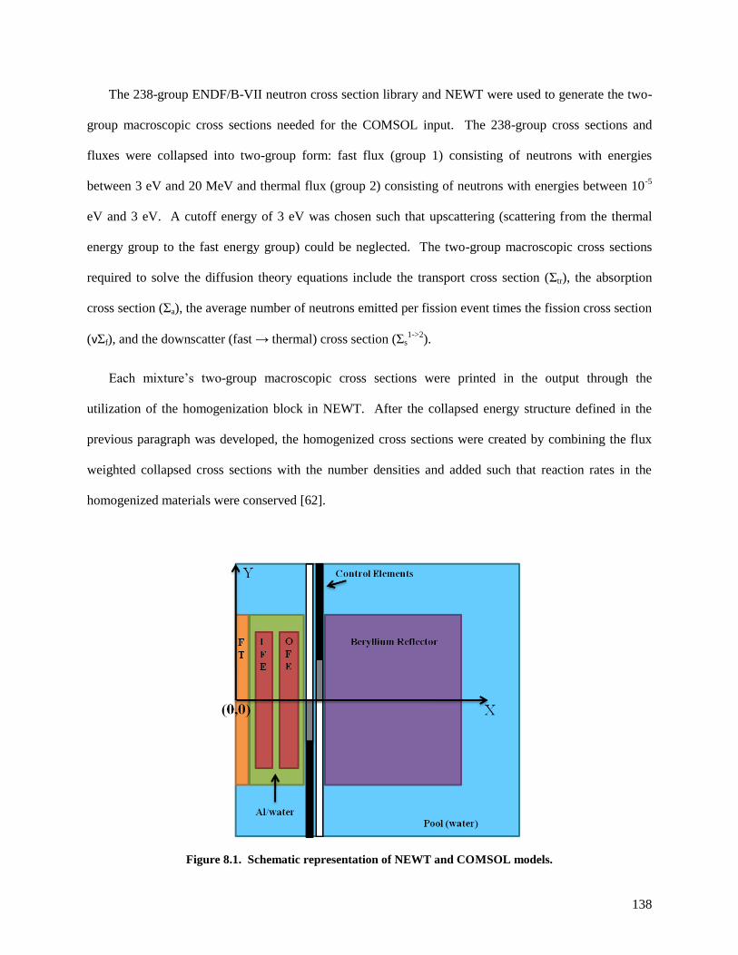
138
The 238-group ENDF/B-VII neutron cross section library and NEWT were used to generate the two-
group macroscopic cross sections needed for the COMSOL input. The 238-group cross sections and
fluxes were collapsed into two-group form: fast flux (group 1) consisting of neutrons with energies
between 3 eV and 20 MeV and thermal flux (group 2) consisting of neutrons with energies between 10-5
eV and 3 eV. A cutoff energy of 3 eV was chosen such that upscattering (scattering from the thermal
energy group to the fast energy group) could be neglected. The two-group macroscopic cross sections
required to solve the diffusion theory equations include the transport cross section (Σtr), the absorption
cross section (Σa), the average number of neutrons emitted per fission event times the fission cross section
(νΣf), and the downscatter (fast → thermal) cross section (Σs1->2
).
Each mixture’s two-group macroscopic cross sections were printed in the output through the
utilization of the homogenization block in NEWT. After the collapsed energy structure defined in the
previous paragraph was developed, the homogenized cross sections were created by combining the flux
weighted collapsed cross sections with the number densities and added such that reaction rates in the
homogenized materials were conserved [62].
Figure 8.1. Schematic representation of NEWT and COMSOL models.
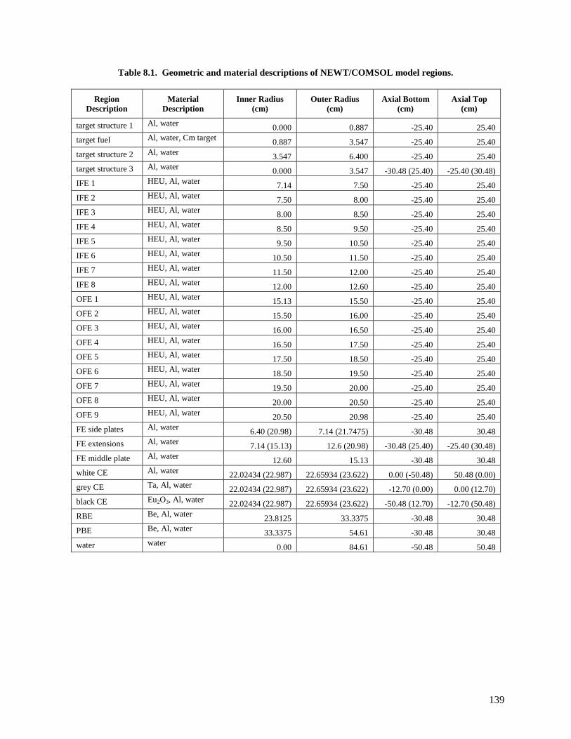
139
Table 8.1. Geometric and material descriptions of NEWT/COMSOL model regions.
Region
Description
Material
Description
Inner Radius
(cm)
Outer Radius
(cm)
Axial Bottom
(cm)
Axial Top
(cm)
target structure 1 Al, water 0.000 0.887 -25.40 25.40
target fuel Al, water, Cm target 0.887 3.547 -25.40 25.40
target structure 2 Al, water 3.547 6.400 -25.40 25.40
target structure 3 Al, water 0.000 3.547 -30.48 (25.40) -25.40 (30.48)
IFE 1 HEU, Al, water 7.14 7.50 -25.40 25.40
IFE 2 HEU, Al, water 7.50 8.00 -25.40 25.40
IFE 3 HEU, Al, water 8.00 8.50 -25.40 25.40
IFE 4 HEU, Al, water 8.50 9.50 -25.40 25.40
IFE 5 HEU, Al, water 9.50 10.50 -25.40 25.40
IFE 6 HEU, Al, water 10.50 11.50 -25.40 25.40
IFE 7 HEU, Al, water 11.50 12.00 -25.40 25.40
IFE 8 HEU, Al, water 12.00 12.60 -25.40 25.40
OFE 1 HEU, Al, water 15.13 15.50 -25.40 25.40
OFE 2 HEU, Al, water 15.50 16.00 -25.40 25.40
OFE 3 HEU, Al, water 16.00 16.50 -25.40 25.40
OFE 4 HEU, Al, water 16.50 17.50 -25.40 25.40
OFE 5 HEU, Al, water 17.50 18.50 -25.40 25.40
OFE 6 HEU, Al, water 18.50 19.50 -25.40 25.40
OFE 7 HEU, Al, water 19.50 20.00 -25.40 25.40
OFE 8 HEU, Al, water 20.00 20.50 -25.40 25.40
OFE 9 HEU, Al, water 20.50 20.98 -25.40 25.40
FE side plates Al, water 6.40 (20.98) 7.14 (21.7475) -30.48 30.48
FE extensions Al, water 7.14 (15.13) 12.6 (20.98) -30.48 (25.40) -25.40 (30.48)
FE middle plate Al, water 12.60 15.13 -30.48 30.48
white CE Al, water 22.02434 (22.987) 22.65934 (23.622) 0.00 (-50.48) 50.48 (0.00)
grey CE Ta, Al, water 22.02434 (22.987) 22.65934 (23.622) -12.70 (0.00) 0.00 (12.70)
black CE Eu2O3, Al, water 22.02434 (22.987) 22.65934 (23.622) -50.48 (12.70) -12.70 (50.48)
RBE Be, Al, water 23.8125 33.3375 -30.48 30.48
PBE Be, Al, water 33.3375 54.61 -30.48 30.48
water water 0.00 84.61 -50.48 50.48

140
The spatial and eigenvalue convergence criteria were both set to 10-4
and coarse-mesh finite-
difference acceleration was activated to speed convergence since there is a significant amount of
scattering in the system [62]. Two options are available in NEWT to set the regions within which
convergence testing is applied: 1) force converged scalar fluxes in every computational cell and 2) relax
convergence such that averaged scalar fluxes within a mixture are converged [62]. The second option is
useful for mixtures in which fluxes become very small (large reflectors or near a vacuum boundary
condition). The second option was used since this model utilizes three vacuum boundary conditions and
includes a large beryllium reflector and water surrounding the core. The NEWT geometry, material
number assignments, and fine rectangular mesh are depicted in Figure 8.2.
Figure 8.2. Grid structure and material placement in NEWT model.

141
8.2 Derivation of Diffusion Theory
The derivation of diffusion theory is based on Fick’s law, which governs that there will be a net flow
of neutrons in a reactor from a region of greater neutron density into a region of lower neutron density
[102], and the equation of continuity, which governs that the net number of neutrons in a nuclear system
must be conserved. The expression for Fick’s law is shown in Equation 8.1 and the expression for
neutron continuity is shown in Equation 8.2. For a complete derivation of these relationships refer to
[100] and [102].
Equation 8.1
where: is the neutron current density vector
D is the diffusion coefficient
is the gradient operator
in rectangular coordinates and
in cylindrical coordinates
ϕ is the neutron flux
Equation 8.2

142
The left-hand side (LHS) of Equation 8.2 represents the time rate of change of the number of neutrons
in volume V. The production rate in V, absorption rate in V, and the net leakage from the surfaces of V
are shown from left to right on the right-hand side (RHS) of Equation 8.2. The diffusion equation is
developed by substituting Fick’s law into the equation of neutron continuity and is shown in Equation 8.3.
Equation 8.3
The focus of this study is to obtain the steady state BOC fluxes, and thus, the time-dependence term
can be neglected. Also, no external sources are present in HFIR, and therefore, fission is the only
contributor to the production rate, S. Thus, the steady state one-group diffusion equation with no external
sources is written in the form of Equation 8.4.
Equation 8.4
Since two energy groups are being studied in this analysis, scattering from one energy group to
another must be included into the diffusion equation. The two-group neutron diffusion equations for fast
(group 1: noted with subscript 1) and thermal (group 2: noted with subscript 2) fluxes assuming all fission
neutrons are born as fast neutrons are shown in Equation 8.5 and Equation 8.6, respectively. The
equations were rearranged such that the LHS of the equations describe the neutron loss mechanism and
the RHS of the equations describe the neutron production mechanism. The effective multiplication factor,
keff, was also inserted to balance the equations and describes how the population of neutrons varies from
one generation to another.
143
Equation 8.5
Equation 8.6
By neglecting upscatter (Σ = 0) and simplifying Equation 8.5 and Equation 8.6 based on the
problem definition of steady state, BOC two-group analysis of HFIR, the following equations are
applicable for the fast flux in the multiplying regions (Equation 8.7), the fast flux in the non-multiplying
regions (Equation 8.8), and the thermal flux in all the regions (Equation 8.9).
Equation 8.7
Equation 8.8
Equation 8.9
Symmetry boundary conditions (BC), vacuum BCs, and continuity BCs are to be applied to the
COMSOL model. A symmetrical BC is governed by Equation 8.10 and shows that the divergence of the
gradient of the neutron flux is equal to zero at the boundary. This BC is used at the core centerline since
only half of the reactor is modeled. A vacuum BC uses the flux slope at the boundary to extrapolate the
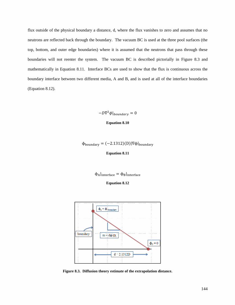
144
flux outside of the physical boundary a distance, d, where the flux vanishes to zero and assumes that no
neutrons are reflected back through the boundary. The vacuum BC is used at the three pool surfaces (the
top, bottom, and outer edge boundaries) where it is assumed that the neutrons that pass through these
boundaries will not reenter the system. The vacuum BC is described pictorially in Figure 8.3 and
mathematically in Equation 8.11. Interface BCs are used to show that the flux is continuous across the
boundary interface between two different media, A and B, and is used at all of the interface boundaries
(Equation 8.12).
Equation 8.10
Equation 8.11
Equation 8.12
Figure 8.3. Diffusion theory estimate of the extrapolation distance.

145
8.3 COMSOL Model Development
The first step in developing a COMSOL model is to select the application mode that is best suited for
the problem being solved. Since COMSOL does not have a built-in neutronics application mode module,
the PDE coefficient application mode and eigenvalue analysis is chosen so the diffusion equations
described in the previous paragraphs can be implemented. The COMSOL model was developed by using
the graphical user interface (GUI) of the COMSOL client to:
a) create the identical geometry that was utilized in the NEWT model,
b) import the macroscopic cross sections previously calculated by NEWT,
c) code the diffusion theory equations into the subdomain settings,
d) define the appropriate boundary conditions in the boundary settings,
e) create an appropriately fine mesh,
f) set up the solver, and finally,
g) perform the actual calculation.
The two-dimensional axisymmetric HFIR COMSOL model as it appears in the draw mode of the GUI
is shown in Figure 8.4. The same dimensions defined in the NEWT model (Table 8.1) were utilized in
the COMSOL model.
The PDE coefficient mode allows the user to enter a system of PDEs into the software in the form
expressed in Equation 8.13. The equations entered in the subdomain settings GUI for the fast flux in the
multiplying regions, the fast flux in the non-multiplying regions, and the thermal flux in all the regions
are shown in Equation 8.14, Equation 8.15, and Equation 8.16, respectively. The subscripts 1 and 2
indicate fast and thermal energy groups, respectively.
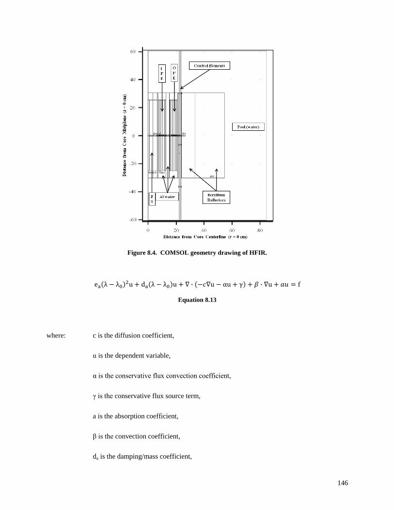
146
Figure 8.4. COMSOL geometry drawing of HFIR.
Equation 8.13
where: c is the diffusion coefficient,
u is the dependent variable,
α is the conservative flux convection coefficient,
γ is the conservative flux source term,
a is the absorption coefficient,
β is the convection coefficient,
da is the damping/mass coefficient,

147
λ is the eigenvalue,
λ0 is the linearization point for the eigenvalue,
ea is the mass coefficient, and
f is the source term.
Equation 8.14
Equation 8.15
Equation 8.16
Two PDE coefficient modes are coupled together and dependent upon each other since the thermal
and fast neutron fluxes are being solved. The dependent variable for the first mode is the fast flux and the
dependent variable for the second mode is the thermal flux. Thus, Equation 8.14 and Equation 8.15 are
input for the multiplying and non-multiplying regions, respectively, in the fast flux PDE coefficient mode
and Equation 8.16 is input for the multiplying and non-multiplying regions in the thermal flux PDE
coefficient mode. Since there are 31 unique materials in the model, there are 31 distinct equations
specified for the fast flux and 31 distinct equations for the thermal flux (62 distinct sets of cross sections
and diffusion coefficients).
148
The boundary conditions were defined in the boundary settings GUI. Boundary conditions were
defined for both the fast and thermal flux physics modes. Symmetry was used at the core axial centerline,
vacuum BCs were applied at the three outer pool boundaries, and continuity BCs were used at all of the
interior interfaces. The governing equations for the boundary conditions are shown in Equation 8.17 -
Equation 8.22. The first equation listed for each BC is written in ―generic‖ terms and the second equation
listed for each BC is the equation applied to the COMSOL model.
Symmetry - Neumann boundary condition:
Equation 8.17
Equation 8.18
Vacuum - Dirichlet boundary condition:
Equation 8.19
Equation 8.20
Continuity - Neumann boundary condition:
Equation 8.21

149
Equation 8.22
COMSOL provides an adaptive mesh refinement algorithm that provides an iterative solution scheme
to update the mesh based on the results from the solution. In this manner, machine accuracy may be
obtained; thus yielding only round-off error left in the solution. The automatic mesh refinement
algorithm was used to solve the diffusion equations using a sequence of refined meshes. The predefined
―extremely coarse‖ triangular mesh was used as the initial mesh and was refined five times by the
―longest edge‖ refinement method. When using the ―longest edge‖ refinement method, the longest edge
of the triangles that are determined to have the largest errors are bisected in order to increase the number
of elements in areas of largest numerical error. The initial mesh was used to solve the system of PDEs
and was improved by computing local mesh element error indicators, (f(i,j)h(j)β(i)
)αVol(j), and refining the
mesh where the errors are largest. The local error indicators depend on the equation number (i), the mesh
element number (j), the mesh element size (h), and the mesh element volume (Vol). The global error is
estimated by taking the sum of the local error estimates. The mesh refinement loop continues until the
maximum number of refinements is reached or the maximum number of elements is obtained, both of
which are user-defined values [65].
Mesh quality, as described in [103], concerns the characteristics of a mesh that permit a particular
numerical PDE simulation to be efficiently performed, with fidelity to the underlying physics, and with
the accuracy required for the problem. The mesh quality influences the convergence, accuracy, and
efficiency of finite-element-based simulations. Since the mesh quality used in COMSOL is based on the
geometry and the aspect ratio of the element and not on the actual physics being solved, the mesh quality
shown is not necessarily an indicator of solution ability. However, the COMSOL documentation [65]
states that if the quality is at least greater than 0.3, then the mesh quality is sufficient to obtain an accurate
solution.

150
The PARDISO direct linear system solver was chosen in the solver parameters dialog box because it
is more efficient and uses less memory than other solvers. The PARDISO solver is a direct solver for
sparse symmetric and unsymmetric linear systems (Ax=b) of equations. In diffusion theory, the A matrix
represents the destruction matrix [leakage, absorption, and downscatter (for the fast flux group only)], x is
the neutron flux, and b is the production vector [fission and downscatter (for the thermal group only)].
Referring to Equation 8.13 through Equation 8.16, static eigenvalue problems in COMSOL are setup
similarly to time-dependent problems by linking the time derivative, ∂ϕ/∂t, to the eigenvalue, λ. Thus, for
a critical system (keff = unity), the eigenvalue is equal to zero according to the set of PDEs being solved,
and therefore, a desired eigenvalue of 0 was defined and the eigenvalue linearization point was set to 0.
8.4 NEWT/COMSOL Two-Group Flux Results
The NEWT code in the SCALE 6 system was used to model HFIR and generate the two-group
macroscopic cross sections needed to solve the diffusion equations by calculating zone-averaged neutron
fluxes and then using them to collapse the 238-group ENDF/B-VII cross section library to a two-group
structure. The effective multiplication factor for the defined configuration was calculated to be 1.0033.
The thermal (10-5
< En < 3 eV) and fast (3 eV < En < 20 MeV) neutron flux distributions as calculated
with NEWT are depicted in Figure 8.5 and Figure 8.6, respectively. In these figures, the neutron flux is
viewed by the color spectrum scale whereby the red color represents the largest flux and the blue
represents the smallest flux. Due to the very fine mesh applied around the CEs, it is difficult to see the
flux profile in and around them. A very fine mesh is needed for the discrete representation of the model
of HFIR since it is a very compact HEU loaded core and there are sharp gradients in the fluxes. The
steepest gradients occur near the edges of the fuel elements where the neutrons are moving from fuel
regions to moderating [water (FT and flow channels) and beryllium] and absorbing (control elements)
regions.

151
The thermal and fast neutron flux distributions as calculated with COMSOL are shown in Figure 8.7
and Figure 8.8, respectively, and are in very good agreement with the NEWT results shown in Figure 8.5
and Figure 8.6. Figure 8.7 and Figure 8.8 are surface plots that show the continuous distribution of the
fluxes. Contour lines overlay these plots to capture the discrete curves of the solution field. Again, the
neutron flux is viewed by the color spectrum scale whereby red represents the largest flux and blue
represents the smallest flux. The square root of the thermal flux is plotted along with the thermal flux
surface plot in Figure 8.7 for the sole purpose of showing more variability in the color spectrum. It is
important to note that the square root of the flux has no physical meaning. As mentioned in the previous
paragraph, steep flux gradients are unique to the compact HFIR core, which are emphasized in Figure 8.7
where the FT is red and all other regions are blue.
Region specific thermal and fast neutron flux surface plots for the FT, FE, CEs, and the beryllium
reflector regions are illustrated in Figure 8.9 through Figure 8.12, respectively. The FT, FE, and
beryllium reflector plots are bounded by the y = -30.48 cm and y = 30.48 cm planes (active fuel length is
only 50.8 cm in length) and the CE surface plot shows the entire length of the elements as modeled. The
width-to-height ratio of the CEs was increased for better visibility of the plot and CE drawings were
placed next to the plots such that the three regions (white, grey, and black) could be easily identified.
Fast neutrons are born in the fuel regions and leak out into the FT and beryllium reflector regions
where they are moderated to lower energies. The fast flux decreases with increasing penetration into the
FT and the beryllium reflector regions because they are being thermalized. The thermal flux increases
with increasing penetration into the FT and is greatest at center of the core. The thermal flux also
increases with increasing penetration into the beryllium reflector and is greatest (in the reflector) at a
distance of approximately 4 cm into the reflector (at the horizontal midplane) and then exponentially
decreases with distance out of the reflector and into the pool.
The fast flux at the horizontal midplane is greatest at the outer edge of the IFE and the inner edge of
the OFE and dips slightly in the region between the FEs since fast neutrons are produced in the fuel
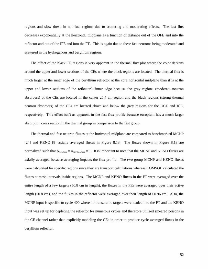
152
regions and slow down in non-fuel regions due to scattering and moderating effects. The fast flux
decreases exponentially at the horizontal midplane as a function of distance out of the OFE and into the
reflector and out of the IFE and into the FT. This is again due to these fast neutrons being moderated and
scattered in the hydrogenous and beryllium regions.
The effect of the black CE regions is very apparent in the thermal flux plot where the color darkens
around the upper and lower sections of the CEs where the black regions are located. The thermal flux is
much larger at the inner edge of the beryllium reflector at the core horizontal midplane than it is at the
upper and lower sections of the reflector’s inner edge because the grey regions (moderate neutron
absorbers) of the CEs are located in the center 25.4 cm region and the black regions (strong thermal
neutron absorbers) of the CEs are located above and below the grey regions for the OCE and ICE,
respectively. This effect isn’t as apparent in the fast flux profile because europium has a much larger
absorption cross section in the thermal group in comparison to the fast group.
The thermal and fast neutron fluxes at the horizontal midplane are compared to benchmarked MCNP
[24] and KENO [8] axially averaged fluxes in Figure 8.13. The fluxes shown in Figure 8.13 are
normalized such that ϕfast,max = ϕthermal,max = 1. It is important to note that the MCNP and KENO fluxes are
axially averaged because averaging impacts the flux profile. The two-group MCNP and KENO fluxes
were calculated for specific regions since they are transport calculations whereas COMSOL calculated the
fluxes at mesh intervals inside regions. The MCNP and KENO fluxes in the FT were averaged over the
entire length of a few targets (50.8 cm in length), the fluxes in the FEs were averaged over their active
length (50.8 cm), and the fluxes in the reflector were averaged over their length of 60.96 cm. Also, the
MCNP input is specific to cycle 400 where no transuranic targets were loaded into the FT and the KENO
input was set up for depleting the reflector for numerous cycles and therefore utilized smeared poisons in
the CE channel rather than explicitly modeling the CEs in order to produce cycle-averaged fluxes in the
beryllium reflector.

153
Although the three models were created for three unique analyses, the flux profiles are in good
agreement with each other. The thermal flux profiles for all three models are consistent with each other,
but there are small discrepancies in the fast flux profiles. These discrepancies can be attributed to
diffusion theory approximations and because the COMSOL-generated fluxes are values along the
horizontal midplane of the core but are being compared to the axially averaged fluxes generated in MCNP
and KENO (see Figure 8.5 - Figure 8.12).
Pertinent mesh data from the COMSOL simulations for the solution based on the initial ―extremely
coarse‖ mesh and each of the 5 iterative solutions are listed in Table 8.2 and include the number of DOF,
the number of mesh points, the number of elements, the minimum element quality, the global error, the
memory usage, and the solution time. During the global adaptive-mesh outer iterations, the number of
DOF, mesh points, and elements increased while the global error decreased. Thus, the accuracy of the
solution is increasing as the mesh is adapting and the memory usage and solution time are increasing.
The mesh quality associated with the initial mesh and the mesh used on the fifth (final) refinement cases
are shown in Figure 8.14. The mesh quality is viewed by the color spectrum scale whereby the red color
represents the highest quality and the blue color represents the lowest quality. In the six cases studied
here, the minimum element quality ranges from 0.438 to 0.529, which is in the green color range.
Compute nodes from an ORNL Research Reactors Division cluster (named Betty) operating on a
Linux platform were used for the calculations described in previous paragraphs. The compute nodes used
for these calculations each have dual AMD Opteron 2350 (2.0 GHz) quad-core 64-bit processors (total of
8 processors per node) and contain 64 GB of ram on each node. Through the utilization of only a single
compute node of the cluster, the solution time for the COMSOL problem with 5 mesh updates was 17.6
minutes. The solution time required to run NEWT to generate the cross sections was approximately 9
hours. This calculation was executed on one of the Betty compute nodes in serial mode. The detailed,
benchmarked, cycle 400 HFIR MCNP5 model (50 million neutron histories) requires approximately 4
hours when running in parallel and distributed over 14 processors (~2.5 days in serial). In comparison, it

154
takes approximately 4 hours of run time for the KENO V.a/CSAS5 and KENO-VI/CSAS6 models of
HFIR to complete when running in serial and simulating 50 million and 1 million neutron histories,
respectively. The SCALE 6.0 code system, including the NEWT and KENO codes, only run in serial
mode, but future releases of SCALE will allow for parallel processing.
After performing the calculations described in the previous paragraphs, the NEWT and COMSOL
models were modified to incorporate a gadolinium rabbit as discussed in Chapter 9 and [104] in the flux
trap target region. Calculations were performed to obtain the cross sections associated with a
representative annular gadolinium shielded rabbit that will be ejected from the hydraulic tube in the near
future. The gadolinium rabbit was inserted into the COMSOL diffusion model at different axial locations
to observe the spatial impact it has on the neutron flux. The thermal (E < 3 eV) flux distributions are
shown in Figure 8.15 for the rabbit at the fuel axial midplane, three quarters the way up the fuel, at the top
of the active fuel, and removed from the core. The presence of the gadolinium rabbit in the flux trap, as
observed in Figure 8.15, reduces the thermal flux in the surrounding area, and thus, shifting the slow
neutrons into the OFE and the beryllium reflector. As the rabbit is ejected, positive reactivity is
nonuniformly introduced into the core as it travels up the hydraulic tube and away from the core.

155
Figure 8.5. NEWT half core thermal neutron flux distribution.

156
Figure 8.6. NEWT half core fast neutron flux distribution.

157
Figure 8.7. COMSOL half core thermal neutron flux distribution.
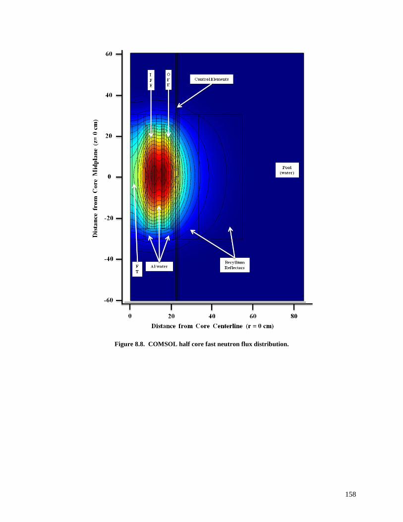
158
Figure 8.8. COMSOL half core fast neutron flux distribution.

159
Figure 8.9. Thermal (middle) and fast (right) flux in the flux trap (h=60.96cm, r=6.4cm).
Figure 8.10. Thermal (middle) and fast (right) flux in the fuel regions (active fuel h=50.8cm).

160
Figure 8.11. Thermal (left) and fast (right) flux in the control elements (h=102cm, w=0.635cm).
Figure 8.12. Thermal (left) and fast (right) flux in the beryllium reflector (h=60.96cm, w=30.80cm).
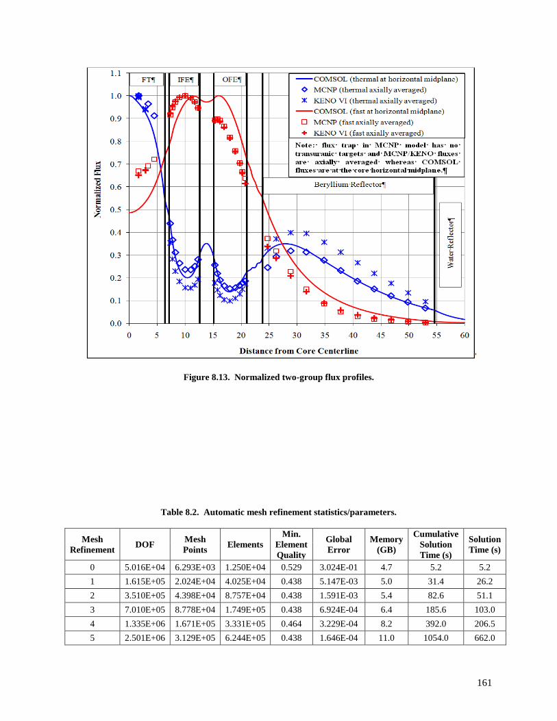
161
Figure 8.13. Normalized two-group flux profiles.
Table 8.2. Automatic mesh refinement statistics/parameters.
Mesh
Refinement DOF
Mesh
Points Elements
Min.
Element
Quality
Global
Error
Memory
(GB)
Cumulative
Solution
Time (s)
Solution
Time (s)
0 5.016E+04 6.293E+03 1.250E+04 0.529 3.024E-01 4.7 5.2 5.2
1 1.615E+05 2.024E+04 4.025E+04 0.438 5.147E-03 5.0 31.4 26.2
2 3.510E+05 4.398E+04 8.757E+04 0.438 1.591E-03 5.4 82.6 51.1
3 7.010E+05 8.778E+04 1.749E+05 0.438 6.924E-04 6.4 185.6 103.0
4 1.335E+06 1.671E+05 3.331E+05 0.464 3.229E-04 8.2 392.0 206.5
5 2.501E+06 3.129E+05 6.244E+05 0.438 1.646E-04 11.0 1054.0 662.0

162
Figure 8.14. COMSOL mesh quality (mesh refinement 0 on left, mesh refinement 5 on right).
Figure 8.15. Thermal flux (E < 3 eV) contour plots during gadolinium rabbit ejection.

163
8.5 Two-Dimensional BOC Static Flux Distribution Summary
A 2-D axisymmetric, two-group, neutron diffusion theory model of HFIR was developed via
COMSOL as a first step approach in creating a spatially-dependent reactor kinetics model. The t-newt
sequence in SCALE version 6 was used to generate the few-group cross sections needed to solve the
diffusion equations and the COMSOL PDE application mode was utilized to solve the diffusion
equations. In Chapter 9, this model is updated by creating a more detailed geometry and by expanding
from two neutron energy groups to three in order to incorporate an epithermal group. A time-dependent
solver will then be setup and spatially-dependent reactivity-induced transients will be studied and
compared to methodologies employing point kinetics.

164
9 Spatially-Dependent and Point Kinetics
In this chapter, the development of COMSOL spatially-dependent and spatially-independent (i.e.,
point) reactor kinetics models is discussed, as well as the response of HFIR’s core during certain
reactivity-induced transients. The models presented in this chapter were developed for the purpose of
studying the spatially-dependent flux/power distribution in the HFIR core during transients caused by
introducing reactivity nonuniformly into the core such that the spatial distribution of the neutron flux
changes during the transient. The results obtained from the spatially-dependent results are then compared
to point kinetics solutions. All previous HFIR kinetics studies have employed the spatially-independent
point kinetics equations, which assume that the spatial distribution of the flux remains unchanged during
a transient; however, the spatial distribution of the flux does change during a transient.
The neutronics models are constructed primarily to examine the spatial distribution of the neutron
flux during reactivity-induced transients and to determine whether the point kinetics approximation is
valid for HFIR. Thus, at this point, it is not intended for the HFIR Safety Analysis Report (SAR) to be
updated as a result of these studies. The space-time models and results presented in this chapter consider
the neutronics behavior only, and therefore, fluid flow and heat transfer physics are not modeled. Parallel
studies utilizing COMSOL for fluid flow and heat transfer analyses are currently being conducted at
HFIR and it is expected that these models will be merged with a neutronics model in the future in order to
create a COMSOL-based multiphysics model of HFIR to enable examination of the fully coupled core
behavior during transients.
Since heat transfer and fluid flow physics are not being implemented, thermal-hydraulic reactivity
feedback contributions are not applied. The main reactivity feedback mechanisms include: changes in
fuel and coolant/moderator temperature, void formation, fuel plate deflection, and changes in coolant
flow. Reactivity feedback from coolant/moderator temperature [Moderator Temperature Coefficient
(MTC)] and fuel temperature [Doppler Temperature Coefficient (DTC)] have a notable effect on the
reactor power during a reactivity insertion accident. HFIR was designed with negative MTCs in the fuel

165
region, positive MTCs in the target region, and negative DTCs. The negative feedback introduced by an
increase in fuel region coolant temperature outweighs the positive feedback introduced by an increase in
target region coolant temperature, and thus, negative reactivity is introduced into the core when the
temperature of the water coolant and fuel increases.
The purpose of this work is not to study every possible transient, but to study the spatially-dependent
neutron fluxes in HFIR’s core during nonuniform reactivity insertion events. Thus, only a few of the
possible transient events are being studied and are discussed here.
9.1 Space-Time Computational Methodology
The spatially-dependent multi-group diffusion equations are defined by Equation 9.1 - Equation 9.4.
The time-dependent neutron diffusion and delayed neutron precursor equations are defined in Equation
9.1 and Equation 9.2, respectively, while the stationary neutron diffusion and delayed neutron precursor
equations are defined in Equation 9.3 and Equation 9.4, respectively. For the purpose of these studies,
three neutron energy groups as listed in Table 9.1 and six groups of delayed neutron precursors are
utilized. Thus, a total of 9 partial differential equations are coupled together for the COMSOL
simulations. For these studies, COMSOL version 4.2 is utilized.
For the stationary problem, the effective neutron multiplication factor, keff, is introduced to balance
the set of equations (for a homogeneous equation) or to yield the correct answer (i.e., to adjust ν to force
an initial critical configuration). The effective multiplication factor is not solved for during the time-
dependent simulation and equilibrium conditions (i.e., keff = 1) should be satisfied prior to initiating a
transient. If the system is forced to be critical at the beginning of the transient, the equations should be
balanced by solving for the initial keff and then using this value as a correction factor of the source of
fission neutrons in the reactor (ks) for the duration of the transient. Thus, for Equation 9.1 and Equation

166
9.2, ks is set to unity when the initial reactor configuration is critical and defined as the keff value
calculated via Equation 9.3 and Equation 9.4 when the initial configuration yields a non unity keff.
Equation 9.1
Equation 9.2
Equation 9.3
Equation 9.4

167
Where the notation is as follows:
= neutron flux for energy group g
= effective neutron multiplication factor (eigenvalue)
ks = correction factor used in transient to render the system critical at t = 0
= average neutron speed for energy group g
= diffusion coefficient for energy group g
= macroscopic absorption cross section for energy group g
= macroscopic scattering cross section from energy group g to group g’
= average number of neutrons emitted per fission reaction times macroscopic fission cross
section for energy group g
= fraction of all fission neutrons emitted per fission in the ith delayed neutron group
= total delayed neutron fraction
= delayed neutron precursor concentration for group i
= decay constant for delayed neutron precursor group i
= fraction of prompt neutrons born into energy group g
= fraction of delayed neutrons from precursor group i born into energy group g

168
Table 9.1. Three-group energy structure.
Group # Group Name Lower Neutron Energy Upper Neutron Energy
1 Fast 100 keV 20 MeV
2 Epithermal 0.625 eV 100 keV
3 Thermal 10-5
eV 0.625 eV
Three studies must be performed in sequential order to solve the neutron diffusion equations with
COMSOL’s PDE application mode. The first study utilizes the eigenvalue solver, which is used to
calculate the static neutron flux distribution. The solution to the eigenvalue problem provides an accurate
spatially-dependent flux distribution; however, the amplitude of the flux is internally normalized. Thus, a
stationary calculation must be carried out to normalize the neutron flux to the initial reactor power. The
stationary solution is then used as the initial conditions for the time-dependent calculations.
9.1.1 Eigenvalue Study
The eigenvalue solver is used to find the solution to eigenvalue problems. In these studies, the
solution from eigenvalue problems are used as sophisticated starting guesses to the nonlinear stationary
problems. Nonlinear stationary and transient problems require educated starting guesses in order to find a
solution. The convergence rate is also dependent on the starting guess, and thus, the solution will
converge faster if the initial guess is close to the solution. The coefficient form eigenvalue equation is
defined in Equation 8.13 and the notation is the same as described in Chapter 8.
The three-group eigenvalue diffusion equation requires that the mass coefficient (ea), the linearization
point (λ0), the conservative flux convection coefficient (α), the conservative flux source term (γ), and the
convection coefficient (β) all be set to zero. Equation 9.5 shows the multi-group diffusion PDE problem
to be solved in the computational domain after setting these terms to zero.

169
Equation 9.5
The coefficients in Equation 9.5 as applicable to the three-group eigenvalue diffusion equation are
defined as follows:
da ≡ damping coefficient
da = 1
u ≡ is the neutron flux column vector:
c ≡ is a diagonal matrix whose diagonal elements are 1/(3 times the macroscopic transport
cross sections):

170
a ≡ is a diagonal matrix whose diagonal elements are the macroscopic removal cross
sections, which are equal to the macroscopic cross sections plus the outscattering macroscopic cross
sections:
f ≡ is the source column vector where each element is equal to the neutron contribution via
fission, delayed neutron precursor decay, and inscatter:
The delayed neutron precursor equation requires that the mass coefficient (ea), the linearization point
(λ0), the diffusion coefficient (c), the conservative flux convection coefficient (α), the conservative flux
source term (γ), and the convection coefficient (β) all be set to zero. Equation 9.6 shows the delayed
neutron precursor PDE problem to be solved in the computational domain after setting these terms to
zero.
Equation 9.6

171
The coefficients in Equation 9.6 as applicable to the delayed neutron precursor equation are as follows:
da ≡ the damping coefficient
da = 1
u ≡ is the delayed neutron precursor column vector:
a ≡ is a diagonal matrix whose diagonal elements are the decay constants
f ≡ is the delayed neutron source column vector where each element is equal to the
delayed neutron fraction times the sum of the fission sources:

172
In the Eigenvalue Study Settings edit field, the number of desired eigenvalues to solve for is set to 6
and a value of zero is specified for which the eigenvalue solver should look for solutions. An eigenvalue
equal to zero as applicable to these studies is analogous to a keff equal to unity; thus, verifying a critical
system. The initial values of the variables solved for are initialized to zero under the Dependent Variables
node. In the Eigenvalue Solver node, the maximum norm scaling method is specified. COMSOL has
three types of internal scaling methods that are used to normalize the eigenvectors and include: the root
mean square (RMS), maximum norm, and mass matrix normalization methods. In these studies, the
maximum norm normalization method is used such that the maximum neutron flux is equal to 1 and the
range of the neutron flux is zero to 1. The direct PARDISO solver, which is discussed in detail in
Chapter 8, is utilized because of its efficiency.
9.1.2 Stationary Study
The solution to the eigenvalue problem is used as a starting guess for the stationary problem, which is
used to calculate the equilibrium conditions that will be used for the initial conditions for the transient
problem. In order to solve for the effective eigenvalue, keff, the eigenvalue problem is recast as a
nonlinear stationary problem. This can be achieved by applying a normalization constraint on the
solution. The two most common constraints used when performing eigenvalue calculations in reactor
physics is to normalize to 1 fission neutron (Equation 9.7) or to a desired power level (Equation 9.8).
Equation 9.7
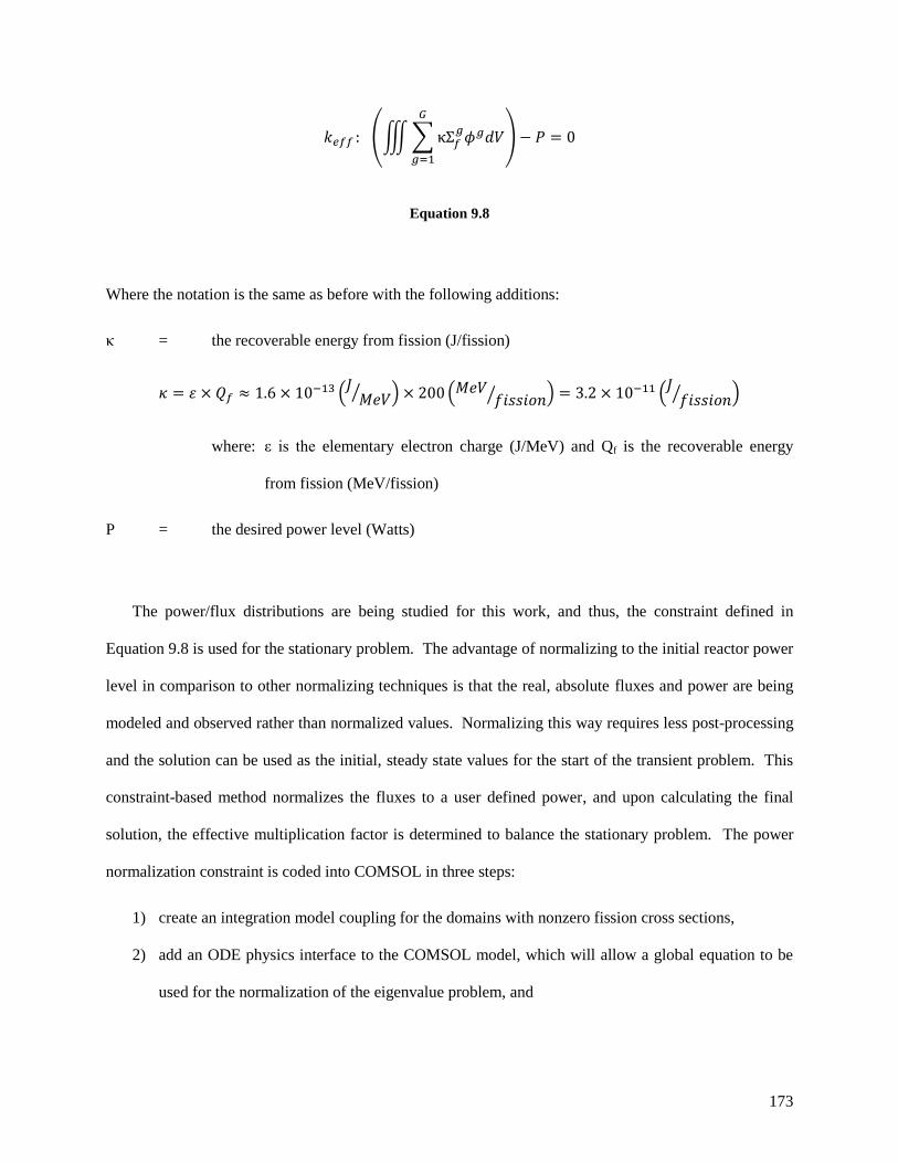
173
Equation 9.8
Where the notation is the same as before with the following additions:
κ = the recoverable energy from fission (J/fission)
where: ε is the elementary electron charge (J/MeV) and Qf is the recoverable energy
from fission (MeV/fission)
P = the desired power level (Watts)
The power/flux distributions are being studied for this work, and thus, the constraint defined in
Equation 9.8 is used for the stationary problem. The advantage of normalizing to the initial reactor power
level in comparison to other normalizing techniques is that the real, absolute fluxes and power are being
modeled and observed rather than normalized values. Normalizing this way requires less post-processing
and the solution can be used as the initial, steady state values for the start of the transient problem. This
constraint-based method normalizes the fluxes to a user defined power, and upon calculating the final
solution, the effective multiplication factor is determined to balance the stationary problem. The power
normalization constraint is coded into COMSOL in three steps:
1) create an integration model coupling for the domains with nonzero fission cross sections,
2) add an ODE physics interface to the COMSOL model, which will allow a global equation to be
used for the normalization of the eigenvalue problem, and

174
3) define keff as the global variable, the constraint (Equation 9.8) as the global expression, and the
initial keff guess as 1.
The stationary coefficient form PDE as solved by COMSOL is shown in Equation 9.9. The three-
group stationary diffusion equation requires that the mass coefficient (ea), the damping coefficient (da),
the conservative flux convection coefficient (α), the conservative flux source term (γ), and the convection
coefficient (β) all be set to zero. Equation 9.10 shows the coefficient form diffusion PDE problem to be
solved in the computational domain after setting these terms to zero. The notation is the same as
described for the eigenvalue calculation.
Equation 9.9
Equation 9.10
In Equation 9.10, u, c, a, and f are again the neutron flux column vector, the diffusion coefficient
diagonal matrix, the macroscopic removal cross section diagonal matrix, and the source column vector,
respectively. After recasting the eigenvalue problem as a stationary problem, the source vector (f) for
both the neutron diffusion and precursor density equations need to be setup to account for keff, and this is
accomplished by replacing the νΣf terms with (νΣf)/keff.

175
f ≡ is the source column vector whose elements are equal to the neutron contribution via
fission, delayed neutron precursor decay, and inscatter:
The result of modifying Equation 9.9 for applicability to the stationary equilibrium delayed neutron
precursor equation is shown in Equation 9.11. Again, u, a, and f refer to the delayed neutron precursor
column vector, the decay constant diagonal matrix, and the delayed neutron source column vector,
respectively, for the six-group delayed neutron precursor equation.
Equation 9.11
The solution from the eigenvalue problem is used as a sophisticated starting guess for the stationary
problem. The spatial distribution (i.e., the shape) of the variables (fluxes and delayed neutron precursor
concentrations) calculated in the eigenvalue study is a good starting point for the stationary case, but the
amplitudes of these variables are orders of magnitude low. The solution to the eigenvalue is normalized
such that the maximum numeric value of the variables is set to one. However, the maximum thermal
neutron flux is known to be approximately 2E+19 neutrons/m2-s in the flux trap, and thus, the initial
starting guess for the stationary problem was defined to be 2E+19 times the eigenvalue solution in the
Initial Values fields of the stationary PDE physics nodes. The solution converges much faster when using
the 2E+19 normalization factor in comparison to using the results ranging from zero to unity. Therefore,

176
the problem was setup with an initial expression/initial value-based method based on the solution from
the eigenvalue problem in the Dependent Variables edit field under the Stationary Solver node. The
PARDISO direct solver was again used to solve the problem.
9.1.3 Transient Study
The stationary problem is solved to obtain the core equilibrium conditions:
a) neutron production = neutron absorption + neutron leakage (i.e., keff = 1) and
b) delayed neutron precursor production rate = delayed neutron precursor destruction rate,
which are used as the initial conditions for the transient problem. For these studies, an initially critical
scenario is sought and Equation 9.1 is solved. If the initial system configuration isn’t a critical
configuration, a correction factor (ks) is used throughout the transient as a constant to satisfy the initial
equations.
The time-dependent coefficient form PDE as solved by COMSOL is shown in Equation 9.12. The
three-group time-dependent diffusion equation requires that the mass coefficient (ea), the conservative
flux convection coefficient (α), the conservative flux source term (γ), and the convection coefficient (β)
all be set to zero. Equation 9.13 shows the coefficient form diffusion theory PDE problem to be solved in
the computational domain after setting these terms to zero.
Equation 9.12

177
Equation 9.13
Where u, c, a, and f are again the neutron flux column vector, the diffusion coefficient diagonal
matrix, the macroscopic removal cross section diagonal matrix, and the source column vector,
respectively. The source column vector takes on the same form as defined in the Stationary Calculation
Section with keff equal to unity for an initially critical configuration. Now:
da ≡ is a diagonal matrix whose diagonal elements are the average neutron inverse velocities
The time-dependent delayed neutron precursor equation requires that the mass coefficient (ea), the
diffusion coefficient (c), the conservative flux convection coefficient (α), the conservative flux source
term (γ), and the convection coefficient (β) all be set to zero. Equation 9.14 shows the coefficient form
delayed neutron precursor PDE problem to be solved in the computational domain after setting these
terms to zero.
Equation 9.14

178
Where u, a, and f are again the delayed neutron precursor column vector, the decay constant diagonal
matrix, and the delayed neutron source column vector, respectively. Now, da takes a value of 1. The
time-dependent delayed neutron precursor equation is a distributed ODE, and thus, has no spatial
derivatives.
The time-dependent solver is setup by defining the times the user wants the solution to be saved and
output and the physics interfaces to be solved under the Time Dependent node. Under the Dependent
Variables node, the initial values for the variables to be solved for are defined as the values of the
variables as calculated from the stationary solver. The time stepping method is setup in the Time-
Dependent Solver node, and for these studies, the BDF (backward differential formula) method is used
and the initial and maximum time steps are adjusted from the default values of 1 ms and 0.1 s,
respectively, to smaller values more appropriate to these studies (~ μs). The time-dependent neutron
diffusion problem can be difficult to solve due the equations being ―stiff,‖ i.e., the time constants
associated with long-lived delayed neutron precursors are large in comparison to the time constants
associated with fast prompt neutrons. The MUMPS direct solver was utilized for the transient
calculations so distributed parallel processing could be utilized.
9.1.4 Boundary Conditions
The same boundary conditions specified in Chapter 8 are used for the neutron flux calculations. Two-
dimensional axisymmetric geometry is used, and thus, symmetry is utilized across the core axial
centerline. Vacuum boundary conditions are defined at the three outer pool edges and continuity
boundary conditions are used across the interior domain interfaces. The boundary conditions are
described pictorially and mathematically (same equations as described in Ch. 8) in Figure 9.1. Note that
the aspect ratio is not preserved in this figure, and thus, the scaling is not representative of reality. Since
the delayed neutron precursor equations have no spatial derivatives and are considered distributed ODEs,
the default zero flux boundary conditions are applied to the outer edges of the fuel domains.

179
Figure 9.1. Neutron flux PDE boundary conditions.
9.2 Point Kinetics Methodology
Reactor point kinetics methodologies are used to predict the response of nuclear reactor cores to
reactivity perturbations. The nuclear data required to solve the point kinetics equations include the
delayed neutron fractions, the delayed neutron precursor decay constants, and the mean generation time.
HFIR’s effective delayed neutron fraction and mean generation time are 0.00762 and 52 μs, respectively,
at BOC conditions. Although increasing computational power and advances in simulation tools support
the application of space-time calculations for more comprehensive analyses, point kinetics will continue
to be utilized in the future because they are computationally efficient and provide quick results.
Reactor point kinetics equations with six delayed neutron precursor groups were also used in this
dissertation to study reactivity-induced transients. Point kinetics was employed with both COMSOL and

180
PARET. The necessary equations were coded into COMSOL via equation based modeling. The point
kinetics equations are derived below starting from the reactor-averaged time-dependent neutron balance
equation (Equation 9.15) and the delayed neutron precursor balance equation (Equation 9.16).
Equation 9.15
Equation 9.16
Point kinetics assumes that the time-dependent neutron flux is separable from the energy and space
domains. Thus, the flux is written as a product of a shape function (ψ) and an amplitude function
(Equation 9.17).
Equation 9.17
The leakage and absorption terms in Equation 9.15 can be removed by introducing the effective
multiplication factor (keff) defined in Equation 9.18.

181
Equation 9.18
After inserting Equation 9.18 into Equation 9.15, the reactor-averaged neutron balance equation can
be written in the form of Equation 9.19. Then, reactivity as defined in Equation 1.5 (ρ = 1 – 1/keff) is
introduced into Equation 9.19 to form Equation 9.20.
Equation 9.19
Equation 9.20
Next, the mean generation time (Λ) is defined in Equation 9.21. This proportionality constant is used
to relate the number of neutrons to the fission rate.
Equation 9.21

182
The point kinetics equations (Equation 9.22 and Equation 9.23) are formed after inserting the mean
generation time into Equation 9.20 and Equation 9.16. Note that n(t) can be replaced with ϕ(t) or P(t) in
the point kinetics equations since they are proportional to each other.
Equation 9.22
Equation 9.23
Where the notation in the above equations is as follows:
n = neutron density
ϕ = neutron flux
P = power
= net leakage of neutrons
ρ = reactivity
βeff = effective delayed neutron fraction
βi = delayed neutron fraction for group i
Λ = mean generation time between birth of a fission neutron and the subsequent absorption leading to
another fission
λi = decay constant for group i

183
Ci = concentration of group i
v = neutron velocity
Via the point kinetics methodology, reactivity feedback from temperature changes in different regions
of the reactor (i.e., fuel, moderator, target rod, target region metal, target region water, annulus water,
control element metal, control element water, etc.) can be taken into account using the ―generic‖
equations defined by Equation 9.24 and Equation 9.25. A temperature coefficient of reactivity (αT) as
defined in Equation 9.24 is equal to the change in reactivity per unit change in temperature (i.e., $/ΔT). If
the coefficient is positive, an increase in temperature will result in an increase in reactivity, and thus, the
reactor power will also increase. However, if the coefficient is negative, an increase in temperature will
result in a decrease in reactivity and in turn will cause the reactor power to decrease. Thus, a reactor
designed with negative temperature coefficients is inherently stable and a reactor with positive
temperature coefficients is inherently unstable. Reactivity feedback from region x can be calculated by
multiplying the temperature coefficient of region x by the change in temperature in region x (i.e.,
Equation 9.25).
Equation 9.24
Equation 9.25

184
Reactivity feedback from fuel region and target region voiding can also be utilized in the point
kinetics methodology by using the appropriate void reactivity coefficients and thermal expansion
coefficients specified in [28] and [29]. Reactivity feedback from changes in temperature and voiding can
be employed in the COMSOL point kinetics model through the use of equation based modeling.
Ordinary differential equations and algebraic equations relating the reactor power to the fuel temperature,
moderator temperature, clad expansion, and etc. can be specified.
9.2.1 PARET Input Description
The PARET code couples neutronic (point kinetics), hydrodynamic (1-D), and heat transfer (1-D)
equations to study nondestructive accidents caused by transients in water-cooled research reactors with
plate- or pin-type fuel elements. In order to represent an accurate power distribution, the HFIR fuel
elements were discretized into 19 axial regions and by dividing the IFE and OFE into 8 and 9 radial
regions, respectively. Each radial region is considered a ―core,‖ which includes a fuel plate plus its
associated coolant channel. Each core has a different power generation, coolant mass flow rate, hydraulic
parameters, and etc. Reactivity feedback is calculated as the sum of the fuel temperature effects, the
moderator density effects, and the fuel plate expansion effects. The modified Runge-Kutta method is
utilized for solving the point kinetics equations and the point-wise contributions are volumetrically
weighted and summed together to yield the total reactivity feedback.
The main PARET inputs include the external reactivity insertion, the thermal properties for the clad
and fuel, the neutronic parameters (6 delayed precursor groups), the operational parameters, and the
control system response data. The PARET input developed in [29] was modified as needed for modeling
the control cylinder ejection transient and the black rabbit ejection tests.

185
9.3 Rate Trip Circuit Analysis
During the black rabbit ejections, the reactor power is measured in units of volts, and thus, the rate
trip circuit must be understood to determine the reactor power in units of watts. The rate trip circuit can
be modeled as a simple RC circuit as shown in Figure 9.2 and the rate trip circuit equations as derived by
Mr. Randy Hobbs, ORNL, are shown below. The reset flux voltage, V(t), which is proportional to the
reactor power level is the input to the circuit. The voltage drop across the resistor, VR(t), is fed to an
operational amplifier with a gain factor of A. Thus, the output voltage to the rate trip comparator,
Vrate(t), is equal to A*VR(t) [Equation 9.26]. The time constant of the system, RC, is equal to 0.25
seconds and the amplifier gain, A, is equal to 10. At 85 MW, the reset flux voltage is 6.67 volts. The
LSSS rate trip circuit voltage according to Equation 9.27 is 3.9235 volts, but the actual rate trip set point
must be set to a lower value to account for instrument uncertainties. The actual rate trip set point that will
scram the reactor is set to a value between 3.11 and 3.16 volts.
Figure 9.2. Rate circuit model.
Rate Circuit Model
V(t)
VR(t)
R
C
Reset FluxVoltage
Amp Vrate(t)= A*VR(t)
To rate TripComparator
186
Equation 9.26
Equation 9.27
Where the value 6.67V/85 MW = 0.07847 V/MW is defined as k. The voltage drop across the resistor,
VR(t), is given by Equation 9.28.
Equation 9.28
And,
Equation 9.29
Therefore, the rate trip output voltage to the trip comparator, Vrate(t), is given by Equation 9.30.
Equation 9.30

187
For an exponential power increase, the reactor power level is governed by Equation 9.31.
Equation 9.31
In Equation 9.31, τ is the reactor period, which is defined as the time required for the reactor power to
change by a factor of e. Rearranging Equation 9.31 and solving for the reactor period yields Equation
9.32.
Equation 9.32
Differentiating the left-hand side (LHS) and the right-hand side (RHS) of Equation 9.31 with respect to
time yields Equation 9.33.
Equation 9.33
By inserting Equation 9.33 into Equation 9.30 and solving for the rate trip output voltage to the trip
comparator yields Equation 9.34.

188
Equation 9.34
9.4 Control Cylinder Ejection Transient
The inner control element is a single cylinder (control cylinder) and is used for regulation purposes.
The control cylinder was not designed to automatically insert during a rapid shutdown, but the reactor
operator has the ability to insert the cylinder if necessary. The outer control element is composed of four
quadrants (safety plates) that are used for both safety and regulation purposes, and are thus scrammable.
Both control elements are composed of multiple regions of various neutron absorbing characteristics: a
white region (Al) that has low absorbing ability, a grey region (Ta-Al) that is 12.7 cm in length and has
moderate absorbing capabilities, and a 55.88 cm long black region (Eu2O3-Al) that has a very high
neutron absorbing ability. During the cycle, the control cylinder moves downward and the safety plates
move upward symmetrically about the horizontal midplane. The black regions are driven away from the
core introducing positive reactivity that compensates for the negative reactivity associated with fuel
burnup. The cylinder and safety plates are driven by an automatic servo system to regulate power and
keep the reactor critical during operation.
During a rapid shutdown (scram), the motion of the control cylinder is stopped since downward
coolant flow and gravity act to drive the control cylinder downwards, which in turn would drive the black
(neutron absorbing) region of the cylinder down and away from the core. Three independent channels are
connected to a magnet coil on each of the four safety plates, and the magnets hold the scram latches in
position. If at least two of the three channels detect any nuclear or process parameters exceeding their
prescribed limits, the safety plates will be released following a delay time (typically ~10 ms) that exists
between the rate trip signal and the release of the safety plates.
189
The safety plates are spring loaded and are inserted with an initial acceleration of four times the
acceleration of gravity, g = 9.807 m/s2. The acceleration decreases linearly from 4 g to 1 g over the first
15.24 cm and then remains 1 g until the safety plates are fully inserted. The downward hydrodynamic
forces caused by downward coolant flow are ignored, and thus, the movement of the safety plates is
conservative; meaning the modeled rate of change of position is slower than reality. The movement of
the safety plates is governed by Equation 9.35 where Δz is the rod displacement in meters, i.e., Δz = |z(t) –
zo|.
Equation 9.35
A reactor power increase of 5 MW over initial power is needed to scram the reactor. The HFIR was
designed with RC network rate trips that include time constants equal to 0.25 seconds (described in
Chapter 8), which is equivalent to a 5 MW jump in power. This design minimizes the chance of an
unplanned shutdown due to electrical noise [30]. The reactor will scram due to a rate of power increase
of approximately 16 MW/s (as well as flux-to-flow, temperature, pressure, etc. set points), but in order to
minimize a scram due to small power spikes, the rate of power increase must be accompanied by an
increase of 5 MW over initial power.
One example of a reactivity-induced transient is the ejection of the control cylinder. The safety plates
cannot be rapidly ejected because of the flow and gravitational forces acting in the downward direction.
However, these downward forces aid in the ejection of the control cylinder following a (possible) failure
in the drive gear system [105]. Upon the gear drive disengaging, the hydrodynamic and gravitational
forces act to drive the black region of the control cylinder away from the core; thus, introducing positive
reactivity and increasing the reactor power. The ejection rate would be slowed down by the hydraulic

190
damping and force equalization cylinder [105]. Detailed analyses were performed during the
development of the HFIR Safety Analysis Report to determine the ejection velocity of the control
cylinder and the frequency of this event. These analyses concluded that the ejection velocity of the
control cylinder would be 0.662 in/sec (1.68148 cm/s) and the frequency was determined to be less than
1x10⁻⁴
per year.
The initial reactor power for the control cylinder ejection is assumed to be 1 kW, which approximates
a zero power condition. The value of 1 kW is justified since this is the typical lowest power level
measured by the fission chambers when the reactor achieves criticality [105]. Low power transients are
of concern because more reactivity is added prior to a scram being initiated, and thus, the lower the initial
reactor power, the greater the peak power relative to the initial power (Pmax/Pinit).
9.4.1 Control Cylinder Ejection Space-Time Methodology
The movements of the control cylinder and safety plates during this transient were previously
described. The transient is initiated by the introduction of positive reactivity due to the withdrawal of the
control cylinder at a rate of 1.68148 cm/s. Once the reactor power level increases to 5 MW over initial
power (5 MW + 1 kW = 5.001 MW), the safety plates are inserted according to Equation 9.35 following a
10 ms delay time. During the time-dependent simulations, the movement of the control elements must be
simulated in order to model the control cylinder ejection transient and to perturb the neutron flux/power
distribution and the reactor power level. Two methods can be used in COMSOL to simulate these
movements and include using the built-in Moving Mesh (ALE) module and defining time- and spatially-
dependent properties.
The ALE module allows boundaries to move based on user-defined input such as a given
displacement, a specified velocity, or as a function of physics parameters. This module adds physics to
the simulation, and thus, increases the number of degrees of freedom and computational time. The mesh
191
within the domain moves/deforms according to the user-defined expressions. The mesh points at domain
interfaces (boundaries) must remain connected, and thus, the mesh within domains bordering the domain
defined to move (i.e., water channels between the control elements) will also deform. Depending on the
problem, the mesh may distort or become inverted requiring the domains to be remeshed.
The ALE module increases the versatility of COMSOL, but is not the best option for simulating the
control element movement needed for this analysis. The control elements are modeled by homogenizing
the aluminum cladding and the control regions, and the modeled width is 6.35 mm. On the outside of
each of the control elements and between them are narrow water channels (~2 – 4 mm). Therefore, the
mesh within these domains quickly become distorted and inverted during the fast and large movements of
the control elements. The simulation can be paused to remesh or COMSOL can be coupled to a
MATLAB script via LiveLink to automatically update the mesh during the simulation.
Based on experience gained during these studies, the most efficient method to implement time-
dependent control element movement is to define time-and axially-dependent properties (i.e., cross
sections). The initial idea of using variable properties instead of the moving mesh was conceived from
[106]. During this webinar, a fluid-structure interaction example was described in which a gate valve was
represented with extremely high viscosity. The as-modeled dimensions of the control elements are 170
cm in length and 6.35 mm in width. Rather than modeling the geometry of each control element as three
separate cylinders (a white, grey, and black region) each with their own set of properties defined as local
(domain-dependent) variables in COMSOL, the geometry of each control element is defined as one single
cylinder. The z-coordinates corresponding to the grey/white and grey/black interfaces are described as
global variables. An illustration showing representative geometries for the control elements is shown in
Figure 9.3.
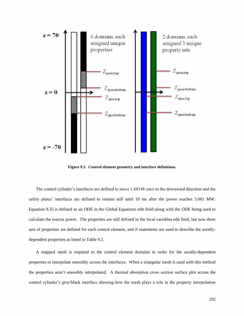
192
Figure 9.3. Control element geometry and interface definitions.
The control cylinder’s interfaces are defined to move 1.68148 cm/s in the downward direction and the
safety plates’ interfaces are defined to remain still until 10 ms after the power reaches 5.001 MW.
Equation 9.35 is defined as an ODE in the Global Equations edit field along with the ODE being used to
calculate the reactor power. The properties are still defined in the local variables edit field, but now three
sets of properties are defined for each control element, and if statements are used to describe the axially-
dependent properties as listed in Table 9.2.
A mapped mesh is required in the control element domains in order for the axially-dependent
properties to interpolate smoothly across the interfaces. When a triangular mesh is used with this method
the properties aren’t smoothly interpolated. A thermal absorption cross section surface plot across the
control cylinder’s grey/black interface showing how the mesh plays a role in the property interpolation

193
between regions is shown in Figure 9.4. The coarse meshes shown in this figure were only used in the
development stages of this methodology; much finer meshes were applied during the calculations
performed and documented here.
The mapped mesh was setup via distributions: 7 radial elements, 100 axial elements above and below
the core region (30.48 –> 70 cm and -30.48 -> -70 cm), and 244 axial elements in the core region. Thus,
a total of 3108 mesh elements were created in each control element. A free triangular mesh was defined
for the remaining geometry; however, different domains were assigned different size meshes. A ―very‖
fine mesh was defined for the water above and below the beryllium reflectors and a ―fine‖ mesh was
assigned to the water on the outside of the beryllium reflector. An ―extremely fine‖ mesh was applied to
all other domains and one further mesh refinement was applied to the fuel and narrow water channels.
The mesh consisted of 6216 quad elements and 64267 triangular elements for a total of 70483 mesh
elements.
Table 9.2. Conditions used to define axially-dependent properties.
If Statement Assigned Properties
z > Zgice,top White Control Cylinder
Zgice,bottom > z > Zgice,top Grey Control Cylinder
z < Zgice,bottom Black Control Cylinder
z > Zgoce,top Black Safety Plates
Zgoce,top > z > Zgoce,bottom Grey Safety Plates
z < Zgoce,bottom White Safety Plates

194
Figure 9.4. Mesh-dependent interface property interpolation (mapped mesh on the left and triangular mesh
on the right)
9.4.2 Control Cylinder Ejection Point Kinetics Methodology
The COMSOL stationary diffusion theory case based on the initial critical configuration was utilized
to determine the worth of the control cylinder during ejection and the worth of the safety plates during
insertion. The control cylinder’s and safety plates’ position vs. time curves were extracted from the
control cylinder ejection transient results and then static cases were run to compute time-dependent
effective multiplication factors, which were converted into reactivity using βeff = 0.00762. The as-
modeled reactivity worth of the control cylinder was determined to be about 85 cents per second or about
51 cents per cm if being ejected at 1.68 cm/s. During these calculations, the safety plates were kept at
their initial position.
The safety plates’ worth was calculated by positioning both control elements at multiple time-
dependent positions, calculating the worth of the configuration with respect to the initial position, and
then subtracting the reactivity worth of the control cylinder. It was determined that the worth of the
safety plates was not linear with respect to time because they are worth more initially when the grey and
black regions are across from the control cylinder’s white region and are worth less when the black region
195
of the safety plates is next to the control cylinder’s black region. The initial and final reactivity worth of
the safety plates was determined to be approximately -55 and -17 cents per cm, respectively.
For the COMSOL-based point kinetics calculations, the control cylinder’s movement was specified as
1.68 cm/s and the worth was specified as 51 cents per second. The movement of the safety plates defined
by Equation 9.35 was specified following a 10 ms response time after the scram set point was reached.
The safety plate worth/cm vs. position curve was inserted into an interpolation table such that the worth of
the safety plates was calculated based on its position. The total reactivity was defined as a global
variable, so at each time point the reactivity was printed in the results table. This reactivity curve was
then discretized and inserted into the PARET input as the externally inserted reactivity as a function of
time.
9.5 Black Rabbit Ejection Transient
The DOE-NE Fuel Cycle R&D Program has requested HFIR assistance in irradiating nuclear fuel
samples to study the microstructural evolutionary changes due to irradiation of fuel materials, fuel-clad
chemical interactions, and etc. [107]. ―Black‖ rabbits containing thermal neutron absorbing shields (Gd,
GdO2, and Eu2O3) and transmission electron microscopy (TEM) discs have been designed for irradiation
in the HFIR hydraulic tube. The insertion or ejection of these ―black‖ rabbits will lead to negative or
positive reactivity insertions, respectively, which have the potential of initiating power transients,
engaging the safety system, and causing unplanned shutdowns.
Rabbits that are referred to as being ―black‖ contain strong neutron absorbing materials. Gadolinium
has been chosen to shield the TEM disks that will be irradiated in the hydraulic tube to study the
temperature and irradiation-dependent behavior of certain fuels. Gadolinium was chosen to maximize the
fast-to-thermal neutron flux ratio in the TEM disks and to keep the heat generation rates within safety
limits. Aluminum rabbits containing annular Gd rods are being ejected in order to define the operating

196
space (i.e., worth of rabbit, position of rabbit, etc.) without causing a reactor shutdown. Calculations are
being performed to support these ejections, but due to the uncertainties associated with the necessary
calculational inputs (rabbit and control element reactivity worths, rabbit ejection position vs. time, control
element movement, etc.), ejection tests must be performed to study the response during these transients.
During these tests, the reset flux, rate network output voltage, and control rod position are being
monitored and recorded via a high speed multichannel data recorder.
Cadmium shielded rabbits (ρ ≈ 8¢) were ejected at the beginning-of-cycle (BOC 429) from various
HT axial positions at low power (P ≈ 12 MWth) and gadolinium shielded rabbits worth 3¢ to 16¢ as
predicted in [104] have been fabricated for ejection tests. During cycle 434 (startup on February 21,
2011), several Gd rabbits were ejected from position number 5 of the hydraulic tube, which is located at
the core horizontal midplane. Rabbits containing a Gd cylinder with a length and outer radius of 3.81 and
0.33 cm, respectively, were ejected at BOC at reactor power levels approximately equal to 12 MW, 24
MW, and 48 MW. Three days into the fuel cycle, rabbits containing 2.54 cm and 2.79 cm length Gd
cylinders were ejected at a power level of approximately 85 MW, which corresponds to full power.
The 2.54, 2.79, and 3.81 cm long Gd cylinders contain approximately 6.87, 7.55, and 10.30 grams of
Gd, respectively. The density of the Gd is 7.9 grams/cm3 and the isotopic composition is listed in weight
percent in Table 9.3. A black rabbit with a 2.992 cm long Gd cylinder is shown next to its radiograph in
Figure 9.5. The white cylinder shown in the x-ray is the Gd rod and the light grey region surrounding the
Gd is the aluminum rabbit housing. A stack of 9 rabbits were ejected during all of these tests. Aluminum
―pusher‖ rabbits were located at the top and bottom of the stack and aluminum ―dummy‖ rabbits were
located in between the ―pusher‖ rabbits and ―black‖ rabbit.
Similar experiments involving the ejection of cadmium shielded rabbits (ρ ≤ 6¢) at low power and
BOC conditions were performed over 40 years ago in 1967 [108]. Although the results are insightful, no
attempt was made to check the reproducibility of the results and the data cannot be reliably extrapolated
to predict the response to rabbits of higher worth at full power and at BOC or end-of-cycle (EOC)
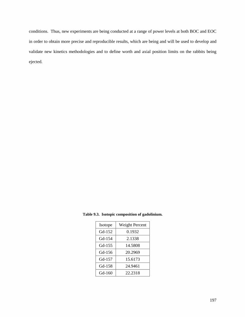
197
conditions. Thus, new experiments are being conducted at a range of power levels at both BOC and EOC
in order to obtain more precise and reproducible results, which are being and will be used to develop and
validate new kinetics methodologies and to define worth and axial position limits on the rabbits being
ejected.
Table 9.3. Isotopic composition of gadolinium.
Isotope Weight Percent
Gd-152 0.1932
Gd-154 2.1338
Gd-155 14.5808
Gd-156 20.2969
Gd-157 15.6173
Gd-158 24.9461
Gd-160 22.2318

198
Figure 9.5. X-ray image of black rabbit RX120R.
9.5.1 Black Rabbit Ejection Space-Time Methodology
The methodology applied to the rabbit ejection studies is similar to that described previously for the
control cylinder ejection analysis. The NEWT input was modified to include a centrally-located
hydraulic tube composed of 6 regions (4 materials). BOC conditions are being studied, and therefore, the
3.81 cm long Gd cylinder was modeled. Since time- and spatially-dependent properties are being defined
to simulate the movement of the rabbit stack, which is displaced with water, it was desired to model the
HT with as few regions as possible. Thus, one region above and below the Gd cylinder was modeled as a
homogenized mixture of aluminum (pusher and dummy rabbits) and water (coolant) and one region above
and below the rabbit stack was modeled as water. The Gd cylinder was explicitly modeled while the
aluminum shield and water coolant were homogenized. A representative illustration of the geometry used
in the NEWT model is shown in Figure 9.6. The figure shown was created from an MCNP input that was
generated with the same geometry and material compositions used in the NEWT input for comparison
purposes.
The exact motion of the rabbits during the ejection is difficult to determine. Prior to ejection, water in
the hydraulic tube is flowing in the downward direction to cool the rabbits and to keep the rabbits in place
and in contact with each other. The flow is then reversed in order to eject the stack of rabbits in the
upward direction. The water flow rate through the hydraulic tube is measured above the core, but
following the cycle 434 ejections, it was determined that the measured flow rate was not representative of

199
the flow through the core because of multiple damaged O-rings and (possibly) a weld from the 1960s that
left a larger than designed gap in the tube. Thus, water was penetrating into the hydraulic tube and the
measured flow was determined to be greater than the flow across the core. Also, inertia effects caused by
the flow rate changing as the water travels around the stack of rabbits will affect the motion of the rabbits.
When the direction of the water is suddenly changed, a shock wave of pressure is exerted in the hydraulic
tube due to water hammer effects that take place when some of the water’s kinetic energy is converted
into pressure. Due to these phenomena, the exact motion of the rabbits is unknown, so parametric point
kinetics studies have been utilized to determine the approximate ejection velocity.
Figure 9.6. Geometry used in black rabbit ejection analysis.

200
The hydraulic tube was defined as one region such that the properties (cross sections, etc.) of the
different materials in the hydraulic tube could be defined as functions of space and time. A representative
depiction of the hydraulic tube is shown in Figure 9.7. The blue regions represent the water regions
above and below the stack of rabbits, the grey regions represent the aluminum rabbits above and below
the Gd cylinder, the red region represents the Gd cylinder, and the green region represents the aluminum
shield.
Similarly to the control cylinder ejection methodology, axial interfaces (shown as z0 – z5) are defined
and if statements are used to assign each region with its appropriate properties [i.e., if(z < z1, water, …)].
Axial locations z0 and z5 remain fixed while the other regions move together in the upward direction and
vanish when they become equal to or greater than z5. A smoothed Heaviside function [i.e., flc2hs(z-
z2,scale)] with a continuous second derivative, provided as a standard function call within COMSOL, was
used to smooth the transition from Gd to Al since Gd is a much greater neutron absorber than Al. Both
the numerical reliability and the convergence are enhanced by defining these transitions this way rather
than using a step function. A 2 mm length scale was used because a mesh element height of 2 mm was
used in the hydraulic tube.
A symmetrical control element position of 47 cm withdrawn (3.81 cm gap between white region of
control elements and core horizontal midplane) was used for initial conditions since this position was the
average starting position for the BOC low power ejections. During the ejection, the control system senses
the increase in power and counteracts the positive reactivity insertion by inserting the control cylinder.
The control cylinder’s response to the ejection (i.e., the delay time) ranged between 20 ms and 90 ms.
The control cylinder’s position during the transient was calculated by normalizing the measured control
cylinder voltage data with the prior and post ejection steady state positions. A polynomial fit of the
position versus time curve was developed and inserted into COMSOL as an algebraic equation. The
method used to move the three regions (white, grey, and black) of the control cylinder is the same as
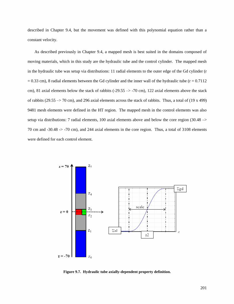
201
described in Chapter 9.4, but the movement was defined with this polynomial equation rather than a
constant velocity.
As described previously in Chapter 9.4, a mapped mesh is best suited in the domains composed of
moving materials, which in this study are the hydraulic tube and the control cylinder. The mapped mesh
in the hydraulic tube was setup via distributions: 11 radial elements to the outer edge of the Gd cylinder (r
= 0.33 cm), 8 radial elements between the Gd cylinder and the inner wall of the hydraulic tube (r = 0.7112
cm), 81 axial elements below the stack of rabbits (-29.55 –> -70 cm), 122 axial elements above the stack
of rabbits (29.55 –> 70 cm), and 296 axial elements across the stack of rabbits. Thus, a total of (19 x 499)
9481 mesh elements were defined in the HT region. The mapped mesh in the control elements was also
setup via distributions: 7 radial elements, 100 axial elements above and below the core region (30.48 –>
70 cm and -30.48 -> -70 cm), and 244 axial elements in the core region. Thus, a total of 3108 elements
were defined for each control element.
Figure 9.7. Hydraulic tube axially-dependent property definition.

202
A boundary layer mesh was applied in the aluminum region located on the outside of the Gd rabbit
because of the sharp flux gradient created in traversing through a heavily water moderated flux trap to a
heavy thermal neutron absorbing material. A free triangular mesh was defined for the remaining
geometry; however, different domains were assigned different size meshes. An ―extra fine‖ mesh was
defined for the permanent beryllium reflector and the water above and below the beryllium reflectors, a
―finer‖ mesh was assigned to the water on the outside of the beryllium reflector and the aluminum
containment structure, and an ―extremely fine‖ mesh was applied to all other domains. Mesh refinement
was applied to the flux trap, fuel, and narrow water channels. The complete mesh consisted of 128796
mesh elements.
9.5.2 Black Rabbit Ejection Point Kinetics Methodology
During preliminary calculations, the positive reactivity generated from the removal of the black rabbit
and the negative reactivity generated from the insertion of the control cylinder was assumed to be linear
over the ejection/insertion time. However, the reactivity worths of the rabbits are greatest at the
horizontal midplane and the control cylinder insertion is not linear. Therefore, a more detailed
methodology was developed following the cycle 434 Gd rabbit ejections and the calculations performed
in References [104] and [109].
For these reactor point kinetics studies, the axial flux shape in the hydraulic tube was used to weight
the importance of each rabbit based on their axial location in the stack of 9 rabbits. The reactivity worth
of the rabbits at the core horizontal midplane with respect to a water filled hydraulic tube was determined
and then these worths were normalized to the axially-dependent weighting factor. The relative neutron
flux at the horizontal midplane is assumed to be unity and the relative flux shape is described by a cosine
function such that the relative flux as a function of axial position is described by Equation 9.36 [110].
The importance weighting factor is calculated by taking the square of the relative flux. The relative flux
is shown pictorially in Figure 9.8.
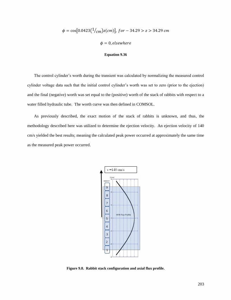
203
Equation 9.36
The control cylinder’s worth during the transient was calculated by normalizing the measured control
cylinder voltage data such that the initial control cylinder’s worth was set to zero (prior to the ejection)
and the final (negative) worth was set equal to the (positive) worth of the stack of rabbits with respect to a
water filled hydraulic tube. The worth curve was then defined in COMSOL.
As previously described, the exact motion of the stack of rabbits is unknown, and thus, the
methodology described here was utilized to determine the ejection velocity. An ejection velocity of 140
cm/s yielded the best results; meaning the calculated peak power occurred at approximately the same time
as the measured peak power occurred.
Figure 9.8. Rabbit stack configuration and axial flux profile.

204
Similarly to the control cylinder methodology, the total reactivity was defined in COMSOL as a
global variable such that the reactivity as a function of time curve was output in the results table. This
reactivity curve was then discretized into approximately 30 pairs and was inserted into the PARET input
as the externally inserted reactivity as a function of time.
9.6 Reactor Kinetics Results
9.6.1 Control Cylinder Ejection Results
A total of 748977 DOF were solved per time step and the solution time was approximately 22 hours.
The MUMPS direct solver was chosen so distributed parallel processing could be utilized. This
calculation was performed across 3 compute nodes, each containing 8 cores on two processors with 64
GB RAM on each compute node.
The symmetrical critical control element position was determined to be about 44.1 cm withdrawn,
which corresponds to a gap of approximately 1 cm between the core midplane and the grey/white region
interface (see Figure 9.3). The initial reactor power was 1.0 kW and the power reached 5.001 MW about
1.365 seconds into the transient. The maximum power of 10.63 MW was achieved 1.390 seconds into the
transient, just 15 ms after the safety plates began moving downward. The pertinent parameters
corresponding to the control cylinder ejection transient are listed in Table 9.4. The reactor power is
plotted as a function of time in Figure 9.9. The control cylinder’s and safety plates’ grey/white region
interface locations are shown along with the reactor power in Figure 9.10. Surface plots of the reactor
power density prior to ejection (t = 0 s), at the time of peak power (t = 1.39 s), and 1.7 seconds after the
transient was initiated are shown in Figure 9.11. More power density surface plots are provided in
Appendix C.
The power derived from the space-time calculation is compared with the point kinetics calculated by
the PARET code and the COMSOL ODE solver in Figure 9.12. The time-dependent worth of the control

205
cylinder ejection was defined as external reactivity in both the PARET and COMSOL inputs. A scram
initiating power and delay time of 5.001 MW and 10 ms, respectively, were defined and the worth of the
safety plates as a function of time after being inserted was specified. As viewed in Figure 9.12, the
maximum power calculated with the PARET model after setting all the feedback coefficients (fuel
temperature, moderator temperature, and void) equal to zero [P(1.39 s) = 10.18 MW] is in good
agreement with the maximum power calculated with the space-time COMSOL model [P(1.39 s) = 10.63
MW].
The maximum power calculated by the PARET model with feedback [P(1.40 s) = 9.70 MW] is
slightly less than the models not employing feedback because HFIR has negative moderator and Doppler
temperature coefficients. Thus, as the reactor power level increases, the fuel and moderator temperatures
increase, which in turn introduces negative reactivity. The maximum power calculated in the COMSOL
point kinetics model (P = 10.10) occurred 1.43 seconds after the transient was initiated. The 0.04 second
difference between the COMSOL space-time and point kinetics models is likely caused by the point
kinetics model assuming no spatial variation in the power distribution. The PARET code is in better
agreement with the space-time results and this is because the PARET model divides the reactor into 323
zones and each zone has a different power generation. In conclusion, the point kinetics methodologies
employed here are sufficient for this analysis as long as local information is not desired.

206
Table 9.4. Summary of space-time control cylinder ejection transient calculation.
Parameter Value Units
to = transient initiation time 0.000 seconds
Po = initial reactor power 1.000 kW
zo,cc = critical CC grey/white region interface location -0.917 cm
zo,sp = critical SP grey/white region interface location 0.917 cm
vcc = velocity of CC 1.681 cm/s
ts = time at P(t) ≥ Po + 5 MW 1.365 seconds
td = delay time (response time) 0.010 seconds
tinsert = time SP begin insertion 1.375 seconds
Pmax = maximum Power 10.628 MW
t(Pmax) = time of maximum Power 1.390 seconds
tsp,fullyinsert = time SP fully inserted 1.538 seconds
ttravel = SP travel time = tsp,fullyinsert - tinsert 0.163 seconds

207
Figure 9.9. Space-time calculated reactor power during control cylinder ejection transient.
1.0E+02
1.0E+03
1.0E+04
1.0E+05
1.0E+06
1.0E+07
1.0E+08
0.0 0.2 0.4 0.6 0.8 1.0 1.2 1.4 1.6 1.8
Rea
ctor
Pow
er (
Watt
s)
Time into Transient (seconds)
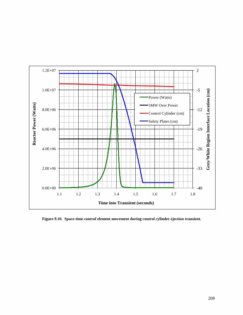
208
Figure 9.10. Space-time control element movement during control cylinder ejection transient.
-40
-33
-26
-19
-12
-5
2
0.0E+00
2.0E+06
4.0E+06
6.0E+06
8.0E+06
1.0E+07
1.2E+07
1.1 1.2 1.3 1.4 1.5 1.6 1.7 1.8
Gre
y/W
hit
e R
egio
n I
nte
rface
Loca
tio
n (
cm)
Rea
ctor
Pow
er (
Wa
tts)
Time into Transient (seconds)
Power (Watts)
5MW Over Power
Control Cylinder (cm)
Safety Plates (cm)
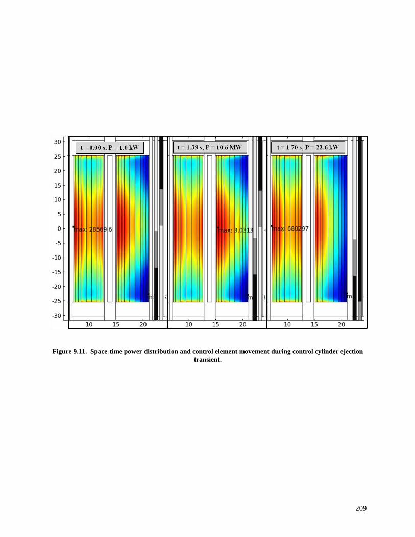
209
Figure 9.11. Space-time power distribution and control element movement during control cylinder ejection
transient.

210
Figure 9.12. Comparison of control cylinder ejection space-time and point kinetics results.
0.00E+00
2.00E+06
4.00E+06
6.00E+06
8.00E+06
1.00E+07
1.20E+07
1.10 1.15 1.20 1.25 1.30 1.35 1.40 1.45 1.50 1.55 1.60
Rea
ctor
Pow
er (
Watt
s)
Time into Transient (seconds)
COMSOL S-T
COMSOL PK
PARET (no FB)
PARET (w FB)
211
9.6.2 Black Rabbit Ejection Results
During the space-time black rabbit ejection simulations, the reactor power level was observed to be
increasing at a much faster rate than expected. There are several reasons that are believed to be causing
this over-prediction in reactor power. The primary explanations include: 1) the few-group nuclear data,
specifically for the Gd cylinder, being calculated by the NEWT representation is not sufficiently accurate
and 2) the limitations of diffusion theory under conditions involving highly absorbing media, sharp flux
gradients, and rapidly time-changing fluxes. The nuclear data are being derived from a 2-D (x, y)
geometric representation of HFIR in NEWT, but the HFIR geometry as modeled in COMSOL is 2-D
axisymmetric (r, z). A detailed investigative study is provided in Appendix D.
The Gd thermal absorption cross section calculated via NEWT is much larger than that calculated by
a comparable 3-D MCNP model. The reactivity worth of the Gd rabbit configuration with respect to a
water filled hydraulic tube is also being over-predicted in NEWT. The measured worth of the
configuration containing a 3.81 cm long Gd cylinder in the central rabbit is -6.98 cents with respect to a
water filled hydraulic tube and the worths predicted from the MCNP model, the NEWT model, the
stationary COMSOL model with the MCNP-derived Gd absorption cross sections, and the stationary
COMSOL model with the NEWT-derived Gd absorption cross sections are -6.59, -27.60, -76.00, and -
107.90 cents, respectively.
A space-time kinetics analysis was performed for an aluminum rod ejection and the change in power
was again over-predicted. The NEWT and MCNP derived macroscopic absorption cross sections for the
aluminum rod were in good mutual agreement, which shows that the three-group neutron diffusion theory
equations implemented in COMSOL is not sufficient to model the hydraulic tube ejections in which the
time-varying flux is being rapidly changed in the center of the reactor core. See Appendix D for more
details regarding these investigative studies.
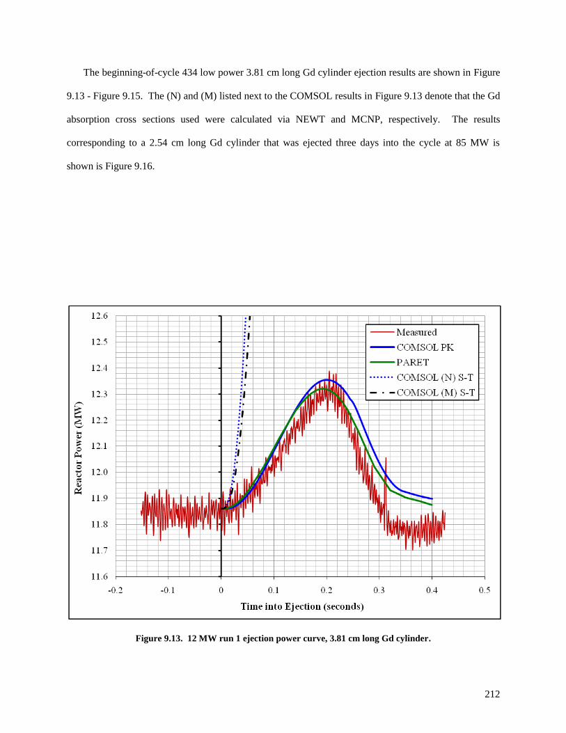
212
The beginning-of-cycle 434 low power 3.81 cm long Gd cylinder ejection results are shown in Figure
9.13 - Figure 9.15. The (N) and (M) listed next to the COMSOL results in Figure 9.13 denote that the Gd
absorption cross sections used were calculated via NEWT and MCNP, respectively. The results
corresponding to a 2.54 cm long Gd cylinder that was ejected three days into the cycle at 85 MW is
shown is Figure 9.16.
Figure 9.13. 12 MW run 1 ejection power curve, 3.81 cm long Gd cylinder.
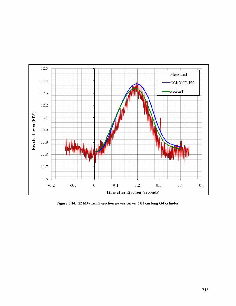
213
Figure 9.14. 12 MW run 2 ejection power curve, 3.81 cm long Gd cylinder.
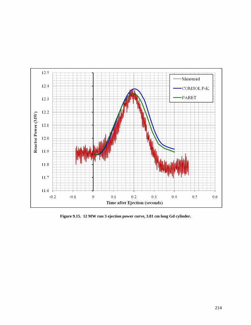
214
Figure 9.15. 12 MW run 3 ejection power curve, 3.81 cm long Gd cylinder.

215
Figure 9.16. 85 MW ejection power curve, 2.54 cm long Gd cylinder.

216
9.7 Reactor Kinetics Summary
Space-time and point kinetics methodologies were developed with the COMSOL and PARET
simulation tools for the purpose of studying HFIR’s response to reactivity-induced transients initiated by
control cylinder and hydraulic tube black rabbit ejections. For the control cylinder ejection transient, the
initial reactor power and the reactor scram set point were specified to be 1 kW and 5.001 MW,
respectively. The space-time and point kinetics models predicted a peak transient power of 10.6 MW and
10.2 MW, respectively, 1.39 seconds after the control cylinder ejection transient was initiated.
The space-time simulation of the hydraulic tube black rabbit ejection greatly over-predicted the
transient reactor power in comparison to the measurements taken and the reactor point kinetics solutions.
The over-prediction is attributed to insufficient few-group nuclear data being derived from a 2-D
representation of HFIR for use in a 2-D axisymmetric representation of HFIR and diffusion theory
limitations near heavy absorbing media and in locations of steep flux gradients. A thorough investigation
is provided in Appendix D.
The reactor point kinetics methodologies developed and employed to study the black rabbit ejections
compared well with the measurements. The ejection velocity was determined to be about 140 cm/s and
the peak transient power occurred approximately 0.20 seconds after the stack of rabbits began moving. A
2.2 MW increase in reactor power was calculated for the 2.54 cm long Gd cylinder ejection at an initial
reactor power of 84.6 MW (2.6 % increase). At an initial power of about 12 MW, a 3.81 cm long Gd
cylinder ejection caused the reactor power to increase approximately 0.5 MW (4.2 % increase). In
conclusion, the reactor point kinetics methodologies developed and described in the previous sections are
sufficiently accurate to predict the HFIR’s response to black rabbit ejections unless localized information
is desired.
217
10 Summary of Conclusions and Suggestions for Future Work
10.1 Summary of Conclusions
The main goal of this research was to develop space-time and point kinetics methodologies for
predicting the dynamic behavior of the HFIR core in response to reactivity-induced perturbations.
Transients initiated by control cylinder and hydraulic tube black rabbit ejections were investigated.
Historically, reactor point kinetics, which assumes that the neutron flux shape is time-independent, has
been used to predict the response of nuclear reactor cores to reactivity perturbations. However, increasing
computational power and advances in simulation tools support the application of space-time calculations
for more comprehensive analyses.
When neutron absorbing materials (i.e., the europium region of the control cylinder on the outside of
the HFIR core and gadolinium rabbits in the center of the HFIR core) are inserted or ejected, reactivity is
introduced which perturbs both the reactor power magnitude and shape. The computational ability to
accurately predict the dynamic behavior of a nuclear reactor core in response to reactivity-induced
perturbations is an important subject in the field of reactor physics, especially from a reactor safety point
of view.
The COMSOL partial differential equation coefficient application mode and 2-D axisymmetric
geometry were utilized to solve the three-group neutron diffusion equations for the purpose of studying
the power/flux distributions during transients such as a control cylinder ejection transient and hydraulic
tube gadolinium rabbit ejections. A total of nine coupled equations were solved: one for each of the three
neutron energy groups (fast, epithermal, and thermal) and one for each of the six delayed neutron
precursor groups. The eigenvalue solver was used to calculate the static neutron flux distribution;
however, the amplitude of the flux is internally normalized, and thus, the eigenvalue problem was recast
as a nonlinear stationary problem by applying a normalization constraint (ODE) on the solution to
normalize the neutron flux to the initial reactor power and to solve for the effective multiplication factor.
218
The stationary solution was then used as the initial conditions for the time-dependent calculations.
During the time-dependent simulations, the movement of the control elements and the rabbits were
simulated by defining time- and spatially-dependent material properties. The PARDISO direct solver was
used for the eigenvalue and stationary problems, but the MUMPS direct solver was used for the transient
calculations in order to utilize distributed parallel processing. The nuclear data required to solve the
space-time kinetics equations were generated by the NEWT code within the SCALE 6 package and
MCNP5.
The space-time models developed in this research only consider the neutronics aspect of reactor
kinetics, and therefore, do not include fluid flow, heat transfer, or reactivity feedback. The research
presented in this dissertation is the first step towards creating a comprehensive multiphysics methodology
for studying the dynamic behavior of the HFIR core during reactivity-induced perturbations. Thermal
hydraulic and structural models are currently being developed in COMSOL at HFIR, and variations of the
three models are expected to eventually be merged together to form a comprehensive multiphysics model.
Both COMSOL and PARET were utilized for the point kinetics calculations. The COMSOL ordinary
differential equation application mode was utilized to solve the reactor point kinetics equations: one
equation for the reactor power and one equation for each of the six groups of delayed neutron precursors.
Global equations and algebraic equations were developed to describe the motion and reactivity worth of
the control elements and stack of rabbits as a function of time. The PARET code couples point kinetics,
1-D heat transfer, and 1-D hydrodynamics to study nondestructive accidents caused by transients in
water-cooled research reactors with plate- or pin-type fuel elements. The PARET model discretizes the
HFIR core into 323 regions (17 radially x 19 axially). Each region has its own power generation and
point-wise contributions are volumetrically weighted and summed together to yield the total reactivity
feedback.
The space-time and point kinetics solutions to the control cylinder ejection transient were found to be
in good mutual agreement. However, at this point, additional effort is required to better implement the

219
space-time black rabbit ejection methodology. The point kinetics models are much more computationally
efficient than the space-time kinetics models and were shown to provide accurate results for small
perturbations in which the power distribution may be assumed to be time-independent (i.e., close to the
steady state distribution). Thus, it has been shown that point kinetics calculations are suitable for
transients involving small perturbations in HFIR’s core unless localized information is desired.
En route to developing the kinetics methodologies, validation studies and methodology updates were
performed to verify the exercise of major neutronic analysis tools at the HFIR. Monte Carlo-based tools
have been shown to be the most appropriate and most powerful tools to perform reactor physics
calculations. Both MCNP and KENO were utilized for these validation studies and methodology updates.
A complex MCNP5 model of HFIR was created by modifying an input for a recent cycle and was
then utilized to validate MCNP for power distribution and effective multiplication factor calculations.
Two sets of critical experiment data were used for these validation studies: a clean core condition (i.e., no
poison in the moderator and control elements at typical beginning-of-cycle positions) and a fully poisoned
core (i.e., 1.35 grams of boron per liter in the moderator to simulate fuel depletion/fission product
poisoning and control elements fully withdrawn). This MCNP model was then modified to replicate the
cycle 4, 16, and 35 configurations and was linked to the ALEPH and VESTA depletion tools. ALEPH
and VESTA were then used to deplete the fuel according to these cycle’s irradiation histories and the
post-irradiation uranium isotopic inventory was compared to mass spectrographic data.
A TRITON/KENO model was developed and used to calculate the buildup and reactivity worth of
helium-3 in the beryllium reflector. Helium-3 is generated and depleted during the cycle, but during an
outage there is no destruction mechanism. A new methodology was developed for predicting the
beginning-of-cycle helium-3 worth and its impact on the estimated symmetrical critical control element
position. This TRITON model was also used to characterize discharged beryllium reflectors, and
specifically permanent beryllium reflector number 3. Uranium is an impurity that exists in beryllium, and
thus, the HFIR reflectors are at risk of becoming transuranic waste. Depletion calculations were
220
performed and proved that permanent beryllium reflector number 3 is transuranic waste and could be
reclassified from hazard category 1 waste to hazard category 3 waste. The TRITON/KENO model was
further modified to calculate the post-irradiation nuclide inventory in 7 curium target rods irradiated in the
flux trap. Dissolver measurements for the californium-252 and berkelium-249 isotopes were shown to be
in good mutual agreement with the calculations.
10.2 Suggestions for Future Work
Although an extensive amount of work has been performed and documented in this dissertation, there
are areas for improvement and suggestions for future work. A few of these research opportunities are
highlighted below:
1. The space-time kinetics methodology described in this research utilized three-group neutron
diffusion theory. However, due to the sharp flux gradients that exist in HFIR, more energy
groups could be used to better predict the power distribution throughout the HFIR core. Thus, the
power distribution could be calculated with more energy groups and compared to the MCNP-
based power distribution in order to optimize the group structure. If the number of energy groups
were to increase, the number of DOF would also increase. This would increase the computational
time and memory consumption, and therefore, iterative solvers and preconditioners would have to
be utilized in order to successfully perform these simulations.
2. Currently, the HFIR geometry is being modeled in two-dimensional axisymmetric geometry such
that symmetry across the axial centerline is being utilized. The geometry could be further
represented by creating a three-dimensional model and incorporating all of the experiment
facilities and the involute fuel plates.
3. If the fuel elements were modeled with involute fuel plates and water coolant channels, then fluid
flow and heat transfer physics could be incorporated into the model. Temperature dependent
221
cross sections would need to be generated if this comprehensive multiphysics model were
developed such that reactivity feedback effects could also be implemented.
4. This dissertation presented a methodology to study the HFIR core behavior during transients
initiated by the movement of the control elements and rabbits in the hydraulic tube, which leaves
the door open to study other transients such as void formations and loss of coolant accidents. The
models described in this dissertation are not currently set up to be able to model these particular
transients, and thus, new methodologies would need to be developed.
There are many areas of research that could come from the space-time kinetics modeling
methodology described in this dissertation. Four areas were briefly discussed as suggestions for future
work, but there are many other ideas that could be investigated.

222
REFERENCES
223
References
[1] D. Chandler, R. T. Primm, III, and G. I. Maldonado, ―Power Distribution Analysis for the ORNL
High Flux Isotope Reactor Critical Experiment 3,‖ Nuclear Science and Engineering, Vol. 164,
January 2010.
[2] D. Chandler, R. T. Primm, III, and G. I. Maldonado, ―Power Distribution Analysis for the High
Flux Isotope Reactor Critical Experiment 3,‖ Transaction American Nuclear Society, Vol. 100,
603 – 604, ANS 2009 Annual Meeting, Atlanta, GA, June 2009.
[3] D. Chandler, R. T. Primm, III, and G. I. Maldonado, ―Validating MCNP for LEU Fuel Design via
Power Distribution Comparisons,‖ ORNL/TM-2008/126, Oak Ridge National Laboratory,
November 2008.
[4] D. Chandler, R. T. Primm, III, and G. I. Maldonado, ―Burnup and Spatially-Dependent Uranium
Isotopic Calculations for the High Flux Isotope Reactor,‖ Transaction American Nuclear Society,
Vol. 103, 768 – 769, ANS 2010 Winter Meeting, Las Vegas, NV, November 2010.
[5] D. Chandler, R. T. Primm, III, and G. I. Maldonado, ―Validation of a Monte Carlo based
depletion methodology via High Flux Isotope Reactor HEU post-irradiation examination
measurements,‖ Nuclear Engineering and Design, Vol. 240, May 2010.
[6] D. Chandler, R. T. Primm, III, and G. I. Maldonado, ―Validation of a Monte Carlo Based
Depletion Methodology Using HFIR Post-Irradiation Measurements,‖ Transaction American
Nuclear Society, Vol. 101, 696 – 698, ANS 2009 Winter Meeting, Washington, D. C., November
2009.
[7] D. Chandler, R. T. Primm, III, and G. I. Maldonado, ―Validation of a Monte Carlo Based
Depletion Methodology with HFIR Post-Irradiation Examination Data,‖ ORNL/TM-2009/123,
Oak Ridge National Laboratory, July 2009.
[8] D. Chandler, R. T. Primm, III, G. I. Maldonado, and L. D. Proctor, ―Nuclear Transmutations in
HFIR’s Beryllium Reflector and Their Impact on Reactor Operation and Reflector Disposal,‖
Accepted for publication in Nuclear Technology.
[9] D. Chandler, R. T. Primm, III, and G. I. Maldonado, ―Classification Calculations for the ORNL
HFIR’s Beryllium Reflector Number 3,‖ Transaction American Nuclear Society, Vol. 103, 676 –
678, ANS 2010 Winter Meeting, Las Vegas, NV, November 2010.
224
[10] D. Chandler, R. T. Primm, III, and G. I. Maldonado, ―Startup Reactivity Accountability
Attributed to Isotopic Transmutations in the Irradiated Beryllium Reflector of the High Flux
Isotope Reactor,‖ Proc. PHYSOR-2010, ANS Topical Meeting on Advances in Reactor Physics
to Power the Nuclear Renaissance, Pittsburgh, PA, May 2010.
[11] D. Chandler and R. T. Primm, III, ―Selected Studies of Past Operations at the ORNL High Flux
Isotope Reactor,‖ Proc. PHYSOR-2010, ANS Topical Meeting on Advances in Reactor Physics
to Power the Nuclear Renaissance, Pittsburgh, PA, May 2010.
[12] D. Chandler, R. T. Primm, III, and G. I. Maldonado, ―Reactivity Accountability Attributed to
Beryllium Reflector Poisons in the High Flux Isotope Reactor,‖ ORNL/TM-2009/188, Oak Ridge
National Laboratory, December 2009.
[13] D. Chandler, R. T. Primm, III, and G. I. Maldonado, ―HFIR Post-Irradiation Curium Target Rod
Nuclide Inventory Calculations,‖ Transaction American Nuclear Society, Vol. 102, 560 – 561,
ANS 2010 Annual Meeting, San Diego, CA, June 2010.
[14] D. Chandler, R. T. Primm, III, G. I. Maldonado, and R. W. Hobbs, ―Black Rabbit Ejection
Studies and COMSOL Kinetics Modeling Development at HFIR,‖ Transaction American Nuclear
Society, Vol. 104, 845 – 847, ANS 2011 Annual Meeting, Hollywood, FL, June 2011.
[15] D. Chandler, R. T. Primm, III, G. I. Maldonado, and J. D. Freels, ―Neutronics Modeling of the
High Flux Isotope Reactor using COMSOL,‖ Accepted for publication in Annals of Nuclear
Energy (2011), doi: 10.1016/j.anucene.2011.06.002.
[16] ―Office of Global Threat Reduction,‖ National Nuclear Security Administration,
<http://nnsa.energy.gov/gtri>.
[17] ―Reduced Enrichment for Research and Test Reactors (RERTR),‖ Office of Nuclear Material
Threat Reduction in the National Nuclear Security Administration, <http://www.rertr.anl.gov>.
[18] ―The National Organization of Test, Research, and Training Reactors (TRTR),‖ The National
Organization of Test, Research, and Training Reactors, <http://www.trtr.org>.
[19] S. C. Mo and J. E. Matos, ―A Neutronic Feasibility Study for LEU Conversion of the High Flux
Isotope Reactor (HFIR),‖ Proc. 1997 International Meeting on Reduced Enrichment for Research
& Test Reactors, Jackson Hole, WY, October 1997.

225
[20] R. T. Primm, III and D. Chandler, ―Preparing the High Flux Isotope Reactor For Conversion to
Low Enriched Uranium Fuel – Extending Cycle Burnup,‖ ANS Topical Meeting ANFM 2009,
Advances in Nuclear Fuel Management IV, Hilton Head Island, SC, April 2009.
[21] J. D. Freels, ―Reactor Point Kinetics Model for HFIR Analysis,‖ C-HFIR-1992-024, Rev. 0,
September 1993, internal, archived publication at the Oak Ridge National Laboratory, contact
Division Director, Research Reactors Division for distribution.
[22] L. Tschaepe, A. E. Ruggles, J. D. Freels, and R. T. Primm, III, ―Evaluation of HFIR LEU Fuel
Using the COMSOL Multiphysics Platform,‖ ORNL/TM-2008/188, Oak Ridge National
Laboratory, March 2009.
[23] N. Xoubi, ―Characterization of Exposure-Dependent Eigenvalue Drift Using Monte Carlo Based
Nuclear Fuel Management,‖ A Dissertation Presented for the Doctor of Philosophy Degree,
University of Cincinnati, November 2005.
[24] R. T. Primm, III and N. Xoubi, ―Modeling of the High Flux Isotope Reactor Cycle 400,‖
ORNL/TM-2004/251, Oak Ridge National Laboratory, August 2005.
[25] G. Ilas and R. T. Primm, III, ―Methodology for Simulating the Irradiation of the Control Elements
in HFIR,‖ Transaction American Nuclear Society, Vol. 103, 696 – 698, ANS 2010 Winter
Meeting, Las Vegas, NV, November 2010.
[26] G. Ilas, J. C. Gehin, and R. T. Primm, III, ―New Cross Section Processing Methodology for HFIR
Core Analysis,‖ Proc. PHYSOR-2008, International Conference on the Physics of Reactors,
Interlaken, Switzerland, September 2008.
[27] R. T. Primm, III, ―Reactor Physics Input to the Safety Analysis Report for the High Flux Isotope
Reactor,‖ ORNL/TM-11956, Oak Ridge National Laboratory, March 1992.
[28] D. G. Morris and M. W. Wendel, ―High Flux Isotope Reactor System RELAP5 Input Model,‖
ORNL/TM-11647, Oak Ridge National Laboratory, February 1993.
[29] C. G. Velit, R. T. Primm, III, and J. C. Gehin, ―Partial Safety Analysis for a Reduced Uranium
Enrichment Core for the High Flux Isotope Reactor,‖ ORNL/TM-2007/226, Oak Ridge National
Laboratory, April 2009.

226
[30] T. Sofu, ―A Model for the Analysis of HFIR Reactivity Transients and Fuel Damage
Propagation,‖ A Dissertation Presented for the Doctor of Philosophy Degree, University of
Tennessee, December 1992.
[31] F. T. Binford, T. E. Cole, and E. N. Cramer, ―The High Flux Isotope Reactor Accident Analysis,‖
ORNL/TM-3573, Oak Ridge National Laboratory, April 1967.
[32] R. D. Cheverton, O. W. Burke, and T. E. Cole, ―HFIR Transients and Reactivity Accountability,‖
ORNL/TM-1747, Oak Ridge National Laboratory, January 1967.
[33] H. L. Dodds, Jr., ―A New Calculational Method for Space-Energy-Angular Dependent Reactor
Kinetics,‖ ORNL/TM-3136, Oak Ridge National Laboratory, A Dissertation Presented for the
Doctor of Philosophy Degree, University of Tennessee, January 1971.
[34] N. J. Ackermann, Jr., ―An Analytical and Experimental Investigation of the Neutron Energy
Effects on Reactor Fluctuation Spectra,‖ ORNL/TM-3245, Oak Ridge National Laboratory, A
Dissertation Presented for the Doctor of Philosophy Degree, University of Tennessee, February
1971.
[35] J. R. Penland, ―Space and Energy Dependence of Reactor Fluctuation Spectra,‖ ORNL/TM-3372,
Oak Ridge National Laboratory, A Dissertation Presented for the Doctor of Philosophy Degree,
University of Tennessee, November 1972.
[36] R. S. Stone and O. W. Burke, ―An Investigation of the Effects of Some Safety System
Modifications on the Safety of the HFIR,‖ ORNL/TM-5738, Oak Ridge National Laboratory,
June 1977.
[37] A. Sozer, ―Component and System Simulation Models for High Flux Isotope Reactor,‖
ORNL/TM-11033, Oak Ridge National Laboratory, August 1989.
[38] D. P. Griggs, M. S. Kazimi, and A. F. Hendry, ―TITAN: an advanced three-dimensional coupled
neutronic/thermal-hydraulics code for light-water nuclear-reactor-core analysis,‖ PB-85-
144251/XAB and MIT/EL-84/011, Massachusetts Institute of Technology, Cambridge, USA,
June 1984.
[39] H. G. Joo, D. Barber, G. Jiang, and T. Downar, ―PARCS: a multi-dimensional two-group reactor
kinetics code based on the nonlinear analytic nodal method,‖ School of Nuclear Engineering,
Purdue University, July 2002.

227
[40] NESTLE Version 5.2.1, ―Few-Group Neutron Diffusion Equation Solver Utilizing The Nodal
Expansion Method for Eigenvalue, Adjoint, Fixed-Source Steady-State and Transient Problems,‖
Electric Power Research Center, North Carolina State University, July 2003.
[41] H. G. Joo, J. Y. Cho, K. S. Kim, C. C. Lee, and S. Q. Zee, ―Methods and Performance of a Three-
Dimensional Whole-Core Transport Code DeCART,‖ Korea Atomic Energy Research Institute,
Proc. PHYSOR-2004, The Physics of Fuel Cycles and Advanced Nuclear Systems: Global
Developments, Chicago, IL, April 2004.
[42] U. Bredolt, ―POLCA-T – Validation of Transient Bundle Flow Predictions During an All
Recirculation Pump-trip in a BWR,‖ Proc. International Conference on Nuclear Engineering 14,
Miami, FL, July 2006.
[43] A. Seubert, K. Velkov, and S. Langenbuch, ―The Time-Dependent 3-D Discrete Ordinates Code
TORT-TD with Thermal-Hydraulic Feedback by ATHLET Models,‖ Proc. PHYSOR-2008,
International Conference on the Physics of Reactors, Interlaken, Switzerland, September 2008.
[44] C. Jönsson, G. Grandi, J. Judd, G. Dominicus, and H. Bergersen, ―Severe Reactivity Initiated
Accidents with SIMULATE-3K and SIMULATE-3K/RELAP5 in Forsmark-3 BWR, Studsvik
Scandpower, Proc. 2010 LWR Fuel Performance/Top Fuel/WRFPM, Orlando, FL, September
2010.
[45] G. Gomes, ―Comparison between COMSOL and RFSP-IST for a 2-D Benchmark Problem,‖
Atomic Energy of Canada Limited, Excerpt from the Proceedings of the COMSOL Conference
2008 Hannover, Hannover, Germany, November 2008.
[46] V. Memoli, A. Cammi, V. D. Marcello, and L. Luzzi, ―A Preliminary Approach to the Neutronics
of the Molten Salt Reactor by means of COMSOL Multiphysics,‖ Politecnico di Milano, Excerpt
from the Proceedings of the COMSOL Conference 2009 Milan, Milan, Italy, October 2009.
[47] ―Nuclear Energy,‖ Ch. 8, 105, The Energy Report, May 2008.
[48] M. W. Rosenthal, ―An Account of Oak Ridge National Laboratory’s Thirteen Nuclear Reactors,‖
ORNL/TM-2009/181, Oak Ridge National Laboratory, August 2009.
[49] R. L. Murray, ―Nuclear Energy An Introduction to the Concepts, Systems, and Applications of
Nuclear Processes,‖ 5th Ed., Woburn, Butterworth Heinemann, 2001.

228
[50] ―Nuclear Power for the Next Generation,‖ International Atomic Energy Agency (IAEA),
<http://www.iaea.org>.
[51] X-5 Monte Carlo Team, ―MCNP—A General Monte Carlo N-Particle Transport Code, Version 5,
LA-CP-03-0245,‖ Los Alamos National Laboratory, April 24, 2003.
[52] RSICC Computer Code Collection CCC-371, ORIGEN 2.2. Available from RSICC, Oak Ridge
National Laboratory, 2002.
[53] I. C. Gauld, O. W. Hermann, and R. M. Westfall, ―ORIGEN-S: SCALE System Module to
Calculate Fuel Depletion, Actinide Transmutation, Fission Product Buildup and Decay, and
Associated Radiation Source Terms,‖ ORNL/TM-2005/39, Version 6, Vol. II, Oak Ridge
National Laboratory, January 2009.
[54] W. Haeck and B. Verboomen, ―ALEPH 1.1.2 – A Monte Carlo Burn-Up Code,‖ SCK-CEN-
BLG-1003, SCK-CEN Belgian Nuclear Research Centre, December 2005.
[55] W. HAECK, ―VESTA User’s Manual – Version 2.0.0‖, IRSN Report DSU/SEC/T/2008-331
Indice A, L'Institut de Radioprotection et de Sûreté Nucléaire (IRSN), France, September 2009.
[56] ―SCALE: A Modular Code system for Performing Standardized Computer Analyses for
Licensing Evaluations,‖ ORNL/TM-2005/39, Version 6, Vols. I - III, Oak Ridge National
Laboratory, January 2009. Available from Radiation Safety Information Computational Center at
Oak Ridge National Laboratory.
[57] S. Goluoglu, N. F. Landers, L. M. Petrie, and D. F. Hollenbach, ―CSAS5: Control Module for
Enhanced Criticality Safety Analysis Sequences with KENO V.A,‖ ORNL/TM-2005/39, Version
6, Vol. I, Oak Ridge National Laboratory, January 2009.
[58] S. Goluoglu, D. F. Hollenbach, and L. M. Petrie, ―CSAS6: Control Module for Enhanced
Criticality Safety Analysis Sequences with KENO-VI,‖ ORNL/TM-2005/39, Version 6, Vol. I,
Oak Ridge National Laboratory, January 2009.
[59] L. M. Petrie, N. F. Landers, D. F. Hollenbach, B. T. Rearden, M. E. Dunn, and S. Goluoglu,
―KENO Va: An Improved Monte Carlo Criticality Program,‖ ORNL/TM-2005/39, Version 6,
Vol. II, Oak Ridge National Laboratory, January 2009.

229
[60] D. F. Hollenbach, L. M. Petrie, S. Goluoglu, N. F. Landers, and M. E. Dunn, ―KENO-VI: A
General Quadratic Version of the KENO Program,‖ ORNL/TM-2005/39, Version 6, Vol. II, Oak
Ridge National Laboratory, January 2009.
[61] M. D. DeHart, ―TRITON: A Two Dimensional Transport and Depletion Module for
Characterization of Spent Nuclear Fuel,‖ ORNL/TM-2005/39, Version 6, Vol. I, Oak Ridge
National Laboratory, January 2009.
[62] M. D. DeHart, ―NEWT: A New Transport Algorithm for Two-Dimensional Discrete Ordinates
Analysis in Non-Orthogonal Geometries,‖ ORNL/TM-2005/39, Version 6, Vol. II, Oak Ridge
National Laboratory, January 2009.
[63] C. F. Obenchain, ―PARET – A Program for the Analysis of Reactor Transients,‖ Phillips
Petroleum Company, US Atomic Energy Commission – Idaho Operations Office, IDO-17282,
January 1969.
[64] A. P. Olson, ―A Users Guide to the PARET/ANL V7.2 Code – Draft, Reduced Enrichment for
Research and Test Reactor (RERTR) Program,‖ Argonne National Laboratory, Argonne, IL, June
2006.
[65] COMSOL: COMSOL, Inc., ―COMSOL Multiphysics User’s Guide,‖ Version 3.5a, Burlington,
MA, November 2008.
[66] COMSOL: COMSOL, Inc., ―COMSOL Multiphysics User’s Guide,‖ Version 4.1, Burlington,
MA, October 2010.
[67] COMSOL: COMSOL, Inc., ―COMSOL Multiphysics User’s Guide,‖ Version 4.2, Burlington,
MA, May 2011.
[68] COMSOL: COMSOL, Inc., ―COMSOL Multiphysics Reference Guide,‖ Version 4.2, Burlington,
MA, May 2011.
[69] R. D. Cheverton and T. M. Sims, ―HFIR Core Nuclear Design,‖ ORNL-4621, Oak Ridge
National Laboratory, July 1971.
[70] S. Goluoglu and H. L. Dodds, “Improved Neutronics Model of the High Flux Isotope Reactor,‖
University of Tennessee, Nuclear Technology, Vol. 112, October 1994.

230
[71] S. G. Goluoglu, H. L. Dodds, and R. B. Rothrock, ―Improved Neutronics Calculations of the
High-Flux Isotope Reactor,‖ ANS Transaction, Vol. 70, 1994.
[72] X-5 Diagnostics Applications Group, ―Data Libraries for MCNP5,‖ CCC-710/MCNP, Los
Alamos National Laboratory.
[73] P. B. Fox and D. F. Hollenbach, ―KENO-VI Validation,‖ ORNL/TM-2004/60, Oak Ridge
National Laboratory, May 2005.
[74] A. E. Richt, R. W. Knight, and G. M. Adamson, Jr., ―Postirradiation Examination and Evaluation
of the Performance of HFIR Fuel Elements,‖ ORNL-4714, Oak Ridge National Laboratory,
December 1971.
[75] JAERI Nuclear Data Center, ―Japanese Evaluated Nuclear Data Library,‖ Version 3, Revision 3,
(JENDL-3.3), Japan Atomic Energy Agency.
[76] R. T. Primm, III, R. J. Ellis, J. C. Gehin, K. T. Clarno, K. A. Williams, and D. L. Moses, ―Design
Study for a Low- Enriched Uranium Core for the High Flux Isotope Reactor, Annual Report for
FY 2006,‖ ORNL/TM-2006/136, Oak Ridge National Laboratory, November 2006.
[77] R. T. Primm, III, D. Chandler, G. Ilas, B. C. Jolly, J. H. Miller, and J. D. Sease, ―Design Study
for a Low-Enriched Uranium Core for the High Flux Isotope Reactor, Annual Report for FY
2008,‖ ORNL/TM-2009/87, Oak Ridge National Laboratory, March 2009.
[78] R. V. McCord and B. L. Corbett, ―OPS EOC 13 Package – HFIR Shutdown Work Schedule,‖
June 12, 1967, internal, archived publication at the Oak Ridge National Laboratory, contact
Division Director, Research Reactors Division for distribution.
[79] R. V. McCord and B. L. Corbett, ―OPS EOC 14 Package – HFIR Shutdown Work Schedule,‖
July 5, 1967, internal, archived publication at the Oak Ridge National Laboratory, contact
Division Director, Research Reactors Division for distribution.
[80] H. L. Dodds, ―OPS EOC 15 Package – HFIR Flux Monitor Runs,‖ September 11, 1967, internal,
archived publication at the Oak Ridge National Laboratory, contact Division Director, Research
Reactors Division for distribution.
[81] ―High Flux Isotope Reactor July, August, and September 1966. Third Quarter 1966,‖ internal,
archived publication at the Oak Ridge National Laboratory, contact Division Director, Research
Reactors Division for distribution.

231
[82] T. A. Tomberlin, ―Beryllium – A Unique Material in Nuclear Applications,‖ Idaho National
Engineering and Environmental Laboratory, Idaho Falls, ID, November 2004.
[83] G. R. Longhurst and R. D. Rohe, ―Beryllium Use in the Advanced Test Reactor,‖ 8th IEA
International Workshop on Beryllium Technology, Lisbon, Portugal, December 2007.
[84] R. T. Primm, III, ―Estimated Symmetrical Critical Control Element Position (ESCCEP) for Cycle
408,‖ C-HFIR-2007-035, May 2007, internal, archived publication at the Oak Ridge National
Laboratory, contact Division Director, Research Reactors Division for distribution.
[85] K. J. Andrzejewski and T. A. Kulikowska, ―Isotopic Transmutations in Irradiated Beryllium and
Their Implications on Maria Reactor Operation,‖ Institute of Atomic Energy, Poland, Nuclear
Technology, Vol. 146, April 2004.
[86] S. Kalcheva, E. Koonen, and B. Ponsard, ―Validation of MCNP & ORIGEN-S 3-D
Computational Model for Reactivity Predictions During BR2 Operation,‖ ISSN 1379-2407, BR2
Division, SCK-CEN, Belgium, January 2005.
[87] ―Radioactive Waste Management,‖ Change 1, DOE O 435.1 U. S. Department of Energy, August
2001.
[88] ―Radioactive Waste Management Manual,‖ DOE M 435.1-1, U. S. Department of Energy, July
1999.
[89] W. Hill, ―Characterization of Permanent Beryllium Reflector Number 3,‖ C-HFIR-2000-071,
February 2001, internal, archived publication at the Oak Ridge National Laboratory, contact
Division Director, Research Reactors Division for distribution.
[90] ―Nevada Test Site Waste Acceptance Criteria,‖ DOE/NV-325-Rev. 7-01, U. S. Department of
Energy, National Nuclear Security Administration, Nevada Site Office, Waste Management
Project, May 2009.
[91] ―Hazard Categorization and Accident Analysis Techniques for Compliance with DOE Order
5480.23, Nuclear Safety Analysis Reports,‖ DOE-STD-1027-92, Change 1, U. S. Department of
Energy, September 1997.
[92] ―Quality Assurance Audit Checklist and Certificate for Use: Procurement and Machining of
HFIR Permanent Be Reflector No. 3,‖ OP-RO-JN-5-1-56, January 1983, internal, archived
publication at the Oak Ridge National Laboratory, contact Division Director, Research Reactors

232
Division for distribution.
[93] ―HFIR Shutdown Work Schedule – End of Cycle 287, EOC 287,‖ November 1986, internal,
archived publication at the Oak Ridge National Laboratory, contact Division Director, Research
Reactors Division for distribution.
[94] C. O. Slater, ―Activation of HFIR HB4 Aluminum Common Casing #1 and Possible Effects on
the Dose to Teflon in the Hydrogen Transfer Line From Alternate Specifications for Aluminum,‖
C-HFIR-2007-029, May 2007, internal, archived publication at the Oak Ridge National
Laboratory, contact Division Director, Research Reactors Division for distribution.
[95] ―Transuranic Waste Acceptance Criteria for the Waste Isolation Pilot Plant,‖ Rev. 6.5,
DOE/WIPP-02-3122, U. S. Department of Energy, June 2010.
[96] ―Licensing Requirements for Land Disposal of Radioactive Waste: Waste Classification, Code of
Federal Regulations,‖ 10 CFR 61.55, U. S. Department of Energy, January 2005.
[97] Personal communication with C. W. Alexander, Oak Ridge National Laboratory, July 20, 2009.
[98] R. D. TAYLOR, ―REDC-TRU73 Transuranium Targets S28, S30, S31, S32, S33, and S34,‖
0059195 REDC-DCN, Oak Ridge National Laboratory, January 2007, internal, archived
publication at the Oak Ridge National Laboratory, contact Division Director, Research Reactors
Division for distribution.
[99] R. D. TAYLOR, ―REDC-TRU73 Transuranium Target S27,‖ 0059112 REDC-DCN, Oak Ridge
National Laboratory, November 2005, internal, archived publication at the Oak Ridge National
Laboratory, contact Division Director, Research Reactors Division for distribution.
[100] W. M. Stacey, ―Nuclear Reactor Physics,‖ John Wiley and Sons, Inc, New York, 2001.
[101] R. T. Primm, III, D. H. Cook, J. D. Freels, G. Ilas, B. C. Jolly, J. H. Miller, D. L. Pinkston, D. G.
Renfro, and J. D. Sease, ―Design Study for a Low-Enriched Uranium Core for the High Flux
Isotope Reactor, Annual Report for FY 2010,‖ ORNL/TM-2011/06, Oak Ridge National
Laboratory, February 2011.
[102] J. R. Lamarsh and A. J. Baratta, ―Introduction to Nuclear Engineering,‖ 3rd
Edition, Prentice Hall,
New Jersey, 2001.

233
[103] P. M. Knupp, ―Remarks on Mesh Quality,‖ Sandia National Laboratory, Paper from the 45th
American Institute of Aeronautics and Astronautics Aerospace Sciences Meeting and Exhibit
2007, Reno, NV, January 2007.
[104] R. J. Ellis, ―Heat Generation and Neutronics Calculations in Support of Black Rabbit
Experiments in HFIR,‖ C-HFIR-2010-011, December 2010, internal, archived publication at the
Oak Ridge National Laboratory, contact Division Director, Research Reactors Division for
distribution.
[105] ―HFIR Updated Safety Analysis Report,‖ ORNL/HFIR/USAR/2344, Rev. 6, Oak Ridge National
Laboratory, Oak Ridge, Tennessee, August 2006.
[106] J. Dunec, ―Fluid-Structure Interaction Simulation with COMSOL,‖ Mechanical Engineering
Magazine Webinar Series Sponsored by COMSOL, March 9, 2011.
[107] R. W. Hobbs and B. F. Siefken, ―High Flux Isotope Reactor (HFIR) Rabbit Ejection Tests,‖
ORNL/HFIR/SBS/2010-01/R0, Oak Ridge National Laboratory, January 2011, internal, archived
publication at the Oak Ridge National Laboratory, contact Division Director, Research Reactors
Division for distribution.
[108] T. M. Sims, ―Results of Preliminary Reactivity Experiments – HFIR Hydraulic Tube,‖ Oak Ridge
National Laboratory, March 1967, contained as an appendix in C. O. Slater and R. T. Primm, III,
―Calculation of Rabbit and Simulator Worth in the HFIR Hydraulic Tube and Comparison with
Measured Values,‖ ORNL/TM-2005/94, Oak Ridge National Laboratory, September 2005.
[109] R. W. Hobbs, ―Reactivity Worth of Rabbits Containing Partial Length Gadolinium Rods or
Sleeves,‖ C-HFIR-2011-007, February 2011, internal, archived publication at the Oak Ridge
National Laboratory, contact Division Director, Research Reactors Division for distribution.
[110] Personal communication with R. W. Hobbs, Oak Ridge National Laboratory, April 5, 2011.
[111] O. Lastres, D. Chandler, J. J. Jarrell, and G. I. Maldonado, ―Studies of Plutonium-238 Production
at the High Flux Isotope Reactor,‖ Transaction American Nuclear Society, Vol. 104, 716 – 718,
ANS 2011 Annual Meeting, Hollywood, FL, June 2011.
[112] ―Start-up Plan for Plutonium-238 Production for Radioisotope Power Systems,‖ Report to
Congress, U. S. Department of Energy, June 2010.

234
[113] J. J. Jarrell, ―Irradiation of 237
Np targets in HFIR,‖ Rev. 1, RNSD-TN-11-001, Internal Technical
Note, Oak Ridge National Laboratory, February 2011.
[114] M. Ragheb, ―Neutron Diffusion Theory,‖ Nuclear, Plasma, and Radiological Engineering,
University of Illinois at Urbana-Champaign, November 2007

235
APPENDICES

236
Appendices
Appendix A – COMSOL PDE Discretization Method
COMSOL uses the Finite Element Method (FEM) to solve problems that can be described in the form
of PDEs. The FEM approximates the solutions to systems of PDEs with problems that have a finite
number of unknown parameters known as degrees of freedom (DOF). The geometry is partitioned into
mesh elements that are connected at node points and bordering mesh elements share the same mesh
edges. The mesh elements are small, simple shapes such that the solution can be approximated using
polynomial interpolations assembled over the mesh elements. Thus, if the solution is known at the node
points, the solution within the mesh element can be interpolated between the node points using the
polynomial basis function. The approximation of the solution improves with the more elements that the
geometry is divided into, but the number of elements also dictates the amount of computational time and
memory (RAM) required to solve the problem. Thus, the mesh needs to be fine enough to be able to
minimize the mesh error, but not too fine such that the problem cannot be solved on the user’s
computational system.
The following description of how COMSOL discretizes the PDEs is paraphrased from [68].
The Lagrange element is the most common type of element used in COMSOL and the order of the
element, k, is the degree of the polynomial function, u. A basis function, υi, and a DOF, Ui, exist at each
node point, pi, and:
Equation A1.
237
The subscript and superscript ɭ in Equation A1 indicate the domain, boundary, or point if equal to 2,
1, or 0, respectively. The constraints, R, on the domain, Ω, the boundary, B, and the points, P, are
discretized such that the constraints must hold point-wise at the Lagrange points, x, with the index of the
mesh element denoted with m:
Equation A2.
The solution vector, U, is composed of the DOF, Ui’s, as its components, and the constraint vector,
M, has the point-wise constraints as its components and depends on U. Thus, M(U) = 0.
In order to discretize the weak equation shown is Equation A3,
Equation A3.
with Lagrange multipliers, μ(i)
, the dependent variables must be expressed in terms of the DOF and the
test functions must be approximated with the same finite elements, i.e., the Galerkin method:
Equation A4.
238
The weak equation holds when the test functions are chosen as the basis functions since the test
functions occur linearly in the integrands of the weak equation:
Equation A5.
Then, define the residual vector, L, as the vector containing the first three terms on the right hand side
of Equation A3:
Equation A6.
Define the Lagrange multipliers as:
Equation A7.
Then, approximate the last three terms on the right hand side of Equation A3 by summing over all the
mesh elements in Ω, B, and P, respectively, and letting the contribution from mesh element number m to
this sum be approximated with the Riemann sum such that:

239
Equation A8.
The integral over Ω and the sum over P are similarly approximated as shown in Equation A8 for the
integral over B. Next, define NF as a matrix composed of a concatenation of the vectors,
. Thus, the discretization of the weak equation can be expressed as:
0 = L - NFΛ
Equation A9.
The discretization of the stationary problem and the time-dependent problem is shown in Equations
A10 and A11, respectively:
0 = L(U) - NF(U)Λ
0=M(U)
Equation A10.
0 = L(U, U’, U’’, t) - NF(U, t)Λ
0=M(U, t)
Equation A11.

240
Appendix B - Plutonium-238 Production Feasibility Study
The study described in this appendix is documented in [111]. The U. S. Department of Energy
(DOE) and the National Aeronautics and Space Administration (NASA) have initiated a plan to restart the
production of 238
Pu for space exploration missions in fiscal year 2011 [112]. Plutonium-238 is an ideal
power source for Radioisotope Thermoelectric Generators (RTG) because it has a very long half life (t1/2
≈ 89 yr) and it generates about 0.5 watts/gram when it decays via alpha emission. An annual production
rate of 1.5 – 2 kg of 238
Pu is expected to satisfy these needs and can be produced in existing national
nuclear facilities like HFIR and the Advanced Test Reactor (ATR) at the Idaho National Laboratory
(INL). Reactors at the Savannah River Site were used in the past for 238
Pu production but were shut down
sometime after the last production occurred in 1988. The nation’s 237
Np inventory is currently stored at
INL [112]
The process of producing 238
Pu includes: (1) fabricating 237
NpOx-Al targets, (2) irradiating the targets
in a nuclear reactor [
], and (3) recovering the 238
Pu in
the targets via chemical extraction. The HFIR complex is ideal for these operations because it is home to
both the reactor, which produces a very high neutron flux for irradiations, and the Radiochemical
Engineering Development Center (REDC), which would be used to perform all of the post-irradiation
processing activities.
At HFIR, 238
Pu production could occur in the vertical experiment facilities (VXF) in HFIR’s
permanent beryllium reflector. Sixteen small (radius = 2.012 cm) and 6 large (radius = 3.599 cm) VXFs
are located within the reflector. The 237
Np target rods (radius = 0.3937 cm and height = 50.8 cm) have
been conceptualized (not yet produced) to hold 35 pellets (radius = 0.3175 cm and height = 1.4478 cm)
with helium as gap filler. The pellets are to be composed of 20 volume % NpOx (impurities include Pu,
Th, U, etc.) in an aluminum matrix. The small and large VXF target bundles are to be assembled in an 8
target polar array and a 31 target triangular array, respectively, as illustrated in Figure B1 [113].
241
This Appendix serves as a feasibility study to better understand the production rates of 238
Pu in HFIR.
VESTA and the ENDF/B-VII continuous energy cross section library were utilized for this study. The
VESTA input was created by modifying the input documented in [25] by modeling the target bundles in
the VXFs and setting up the appropriate irradiation/decay history. The fuel elements in the VESTA input
are divided into 19 axial regions since fuel burnup and control element withdrawal (10 control element
positions/burnup steps) are simulated as a function of cycle time. Rather than modeling 35 pellets in each
target, the target rods were modeled as a single pin within the Al clad. Each target pin was assigned a
different material number such that each target pin was depleted individually. The targets were irradiated
for 24 days, which is a ―typical‖ HFIR cycle length.
The single-cycle 238
Pu production rates in one small VXF array (8 targets) and one large VXF array
(31 targets) as calculated with VESTA are shown in Figure B2. For a 24 day cycle starting with fresh
targets, the VESTA calculation shows that 10.8 and 15.1 grams of 238
Pu can be produced in a small and
large VXF array, respectively. The conversion ratio (ratio of final 238
Pu mass to initial 237
Np mass) is
about 2 % and 5 % in the large and small VXF, respectively. The production rate does not scale
proportionately with the number of targets because the large VXF array is more tightly packed (self-
shielding effects) and further from the core (lower fluxes) in comparison to the small VXF array. The
individual target rod production rates are illustrated in Figure B3 where the axes denote the location of the
pin in cm and the color scale denotes the amount of 238
Pu in grams produced per target rod. The targets
closest to the core can potentially have production rates as high as 3 times of those pins away from the
core, which implies that a cycle-to-cycle rotation of the targets would be necessary. The beginning-of-
cycle and end-of-cycle reactivity worth of one large and one small VXF target array loaded core with
respect to an unloaded core and as calculated with VESTA/MCNP5 are -0.5 and -1.8 ± 2 to 3 cents,
respectively.

242
Figure B1. Cross-sectional view of the HFIR illustrating the small (lower left) and large (upper left) VXF
target arrays simulated in this study.

243
Figure B2. Estimated single-cycle 238
Pu production.
Figure B3. Spatial dependency of 238
Pu production in large VXF (top) and small VXF (bottom).
0
2
4
6
8
10
12
14
16
0 5 10 15 20 25 30 35 40 45 50
Pu
-23
8 (
gra
ms)
Time into Cycle (24 days irradiation + decay)
Large VXF
Small VXF

244
Appendix C – Additional Space-Time Kinetics Figures
This appendix provides additional figures from Chapter 9. Figures C1 – C14 show the power
distribution in the fuel elements during the control cylinder ejection transient. The position of the control
elements are shown to the right of the surface plots.
Figure C1. Power density 0.00 seconds into
control cylinder ejection transient.
Figure C3. Power density 1.00 seconds into
control cylinder ejection transient.
Figure C2. Power density 0.50 seconds into
control cylinder ejection transient.
Figure C4. Power density 1.3653 seconds into
control cylinder ejection transient.

245
Figure C5. Power density 1.3753 seconds into
control cylinder ejection transient.
Figure C7. Power density 1.3903 seconds into
control cylinder ejection transient.
Figure C6. Power density 1.3853 seconds into
control cylinder ejection transient.
Figure C8. Power density 1.40 seconds into
control cylinder ejection transient.

246
Figure C9. Power density 1.41 seconds into
control cylinder ejection transient.
Figure C11. Power density 1.45 seconds into
control cylinder ejection transient.
Figure C10. Power density 1.42 seconds into
control cylinder ejection transient.
Figure C12. Power density 1.50 seconds into
control cylinder ejection transient.

247
Figure C13. Power density 1.60 seconds into
control cylinder ejection transient.
Figure C14. Power density 1.70 seconds into
control cylinder ejection transient.

248
Appendix D – MCNP, NEWT, and COMSOL Neutronics Analyses
This appendix serves to compare certain neutronics parameters such as the effective multiplication
factor, few-group fluxes, and macroscopic absorption cross sections as calculated with MCNP, NEWT,
and COMSOL. The purpose of this appendix is to investigate the rationale behind the unsuccessful
attempt of modeling the black rabbit ejection via the space-time kinetics methodology described in
Chapter 9. The differences in the three computational tools are well documented throughout this
dissertation, but the main differences between the three codes are highlighted in Table D1. For the
studies shown in this appendix, the same geometry and material compositions were used for the MCNP
and NEWT comparisons. Unless specified otherwise, the COMSOL model utilized cross sections
calculated by NEWT.
For the comparisons shown here, three different stationary cases were analyzed. The geometry for all
three cases is identical except for the hydraulic tube configuration. The first case has an aluminum rabbit
housing a 3.81 cm long Gd cylinder at the core midplane and 4 aluminum rabbits above and below the Gd
rabbit. A stack of 9 aluminum rabbits homogenized with water coolant is modeled in the second case and
a water filled hydraulic tube is modeled in the third. An illustration of the three configurations is shown
in Figure D1.
Table D1. MCNP, NEWT, COMSOL neutronic methods.
Code Dimensions Method Data
MCNP 3-D (x, y, z) Stochastic Continuous Energy ENDF/B-VII
NEWT 2-D (x, y) Discrete-ordinates 238-group ENDF/B-VII
COMSOL 2-D axisymmetric (r, z) 3-group diffusion theory 3-group data derived from NEWT

249
Figure D1. Gd rabbit (left), Al stack (middle), and water filled (right) hydraulic tube configurations.
The effective multiplication factors, keff, corresponding to the Gd rabbit and water filled hydraulic
tube configurations as calculated with MCNP, NEWT, and COMSOL are listed in Table D2. Two
COMSOL cases were run for the configuration with the Gd rabbit: one with Gd absorption cross sections
as calculated with NEWT (N) and one with Gd absorption cross sections as calculated with MCNP (M).
The MCNP calculation predicts the worth of the Gd rabbit configuration with respect to the water filled
hydraulic tube within 6 % of the measured value, but the NEWT calculation is almost 300 % off. The
COMSOL-based three-group diffusion theory calculations greatly over-predict the worth of the Gd rabbit.
The three-group Gd macroscopic absorption cross sections as calculated in both MCNP and NEWT
are listed in Table D3. The fast-group cross sections are within 1.4 % of each other, but the epithermal
and thermal groups differ significantly. The NEWT model over-predicts the epithermal and thermal cross
sections by 47 % and 872 % (almost an order of magnitude) in comparison to the MCNP model.

250
Table D2. Worth of Gd rabbit configuration with respect to water filled configuration.
Case Water Filled Gd Rabbit %
Difference keff keff worth ¢
Measured - - -6.98 -
MCNP 1.01763 1.01711 -6.59 -5.54
NEWT 1.01110 1.00896 -27.60 295.39
COMSOL (N) 1.01701 1.00857 -107.90 1445.91
COMSOL (M) 1.01701 1.01105 -76.00 988.88
Table D3. Gd cylinder macroscopic absorption cross sections (1/cm).
Group NEWT MCNP 100(M-N)/M
thermal 9.842E+02 1.012E+02 -872.46
epithermal 5.614E-01 3.821E-01 -46.92
fast 3.807E-03 3.755E-03 -1.38

251
The average three-group neutron fluxes in the Gd cylinder as calculated in MCNP are compared to
the fluxes calculated in COMSOL in Table D4. The epithermal and fast neutron fluxes calculated in both
COMSOL cases are between 1.5 and 2 times less than those calculated with the MCNP model. When
using the absorption cross sections calculated with the NEWT model, the MCNP and COMSOL thermal
neutron flux differs by a factor of 21.6. When the absorption cross sections calculated with MCNP are
used, the thermal flux differs by a factor of 3.4. The COMSOL three-group diffusion theory model
under-predicts the neutron fluxes in the Gd cylinder for all three energy groups.
The COMSOL-derived neutron fluxes are being under-predicted in the Gd cylinder and the worths of
the Gd cylinder are being over-predicted. Thus, the power distribution throughout the reactor core is most
likely not being well calculated. The power distributions as calculated with MCNP, NEWT, and
COMSOL are shown in Figure D2 for the Gd rabbit configuration. The MCNP and NEWT power
distribution are similar except that the NEWT model is slightly under-predicting the power in the IFE and
slightly over-predicting the power in the OFE in comparison to the MCNP model. The difference is
likely due to effect of the Gd rabbit since the NEWT model over-predicts the worth of the Gd rabbit by a
factor of 4. The COMSOL model under-predicts the power at the inner and outer edges of the IFE and
OFE and over-predicts the power in the interior of the IFE and OFE.
Table D4. Neutron flux (neutrons/cm2-s) in Gd cylinder.
Group MCNP COMSOL (N) M/[C(N)] COMSOL (M) M/[C(M)]
thermal 3.129E+13 1.45E+12 21.57 9.22E+12 3.40
epithermal 1.035E+15 5.26E+14 1.97 5.81E+14 1.78
fast 1.055E+15 5.74E+14 1.84 5.79E+14 1.82
total 2.122E+15 1.10E+15 1.93 1.17E+15 1.82
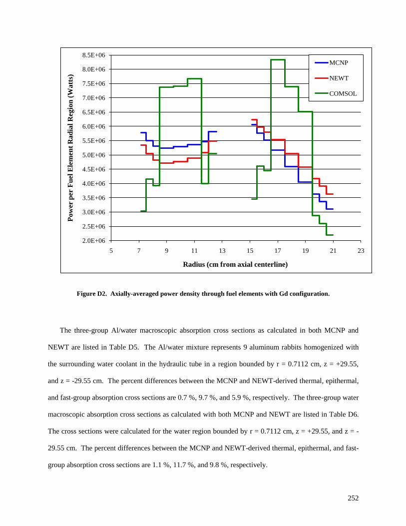
252
Figure D2. Axially-averaged power density through fuel elements with Gd configuration.
The three-group Al/water macroscopic absorption cross sections as calculated in both MCNP and
NEWT are listed in Table D5. The Al/water mixture represents 9 aluminum rabbits homogenized with
the surrounding water coolant in the hydraulic tube in a region bounded by r = 0.7112 cm, z = +29.55,
and z = -29.55 cm. The percent differences between the MCNP and NEWT-derived thermal, epithermal,
and fast-group absorption cross sections are 0.7 %, 9.7 %, and 5.9 %, respectively. The three-group water
macroscopic absorption cross sections as calculated with both MCNP and NEWT are listed in Table D6.
The cross sections were calculated for the water region bounded by r = 0.7112 cm, z = +29.55, and z = -
29.55 cm. The percent differences between the MCNP and NEWT-derived thermal, epithermal, and fast-
group absorption cross sections are 1.1 %, 11.7 %, and 9.8 %, respectively.
2.0E+06
2.5E+06
3.0E+06
3.5E+06
4.0E+06
4.5E+06
5.0E+06
5.5E+06
6.0E+06
6.5E+06
7.0E+06
7.5E+06
8.0E+06
8.5E+06
5 7 9 11 13 15 17 19 21 23
Pow
er p
er F
uel
Ele
men
t R
ad
ial
Reg
ion
(W
att
s)
Radius (cm from axial centerline)
MCNP
NEWT
COMSOL
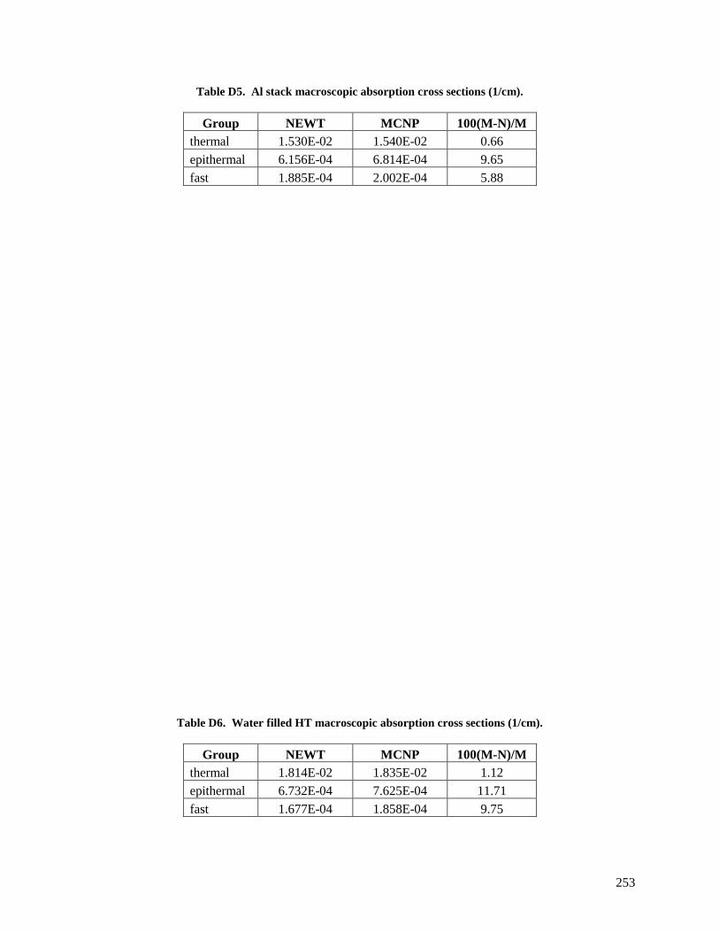
253
Table D5. Al stack macroscopic absorption cross sections (1/cm).
Group NEWT MCNP 100(M-N)/M
thermal 1.530E-02 1.540E-02 0.66
epithermal 6.156E-04 6.814E-04 9.65
fast 1.885E-04 2.002E-04 5.88
Table D6. Water filled HT macroscopic absorption cross sections (1/cm).
Group NEWT MCNP 100(M-N)/M
thermal 1.814E-02 1.835E-02 1.12
epithermal 6.732E-04 7.625E-04 11.71
fast 1.677E-04 1.858E-04 9.75
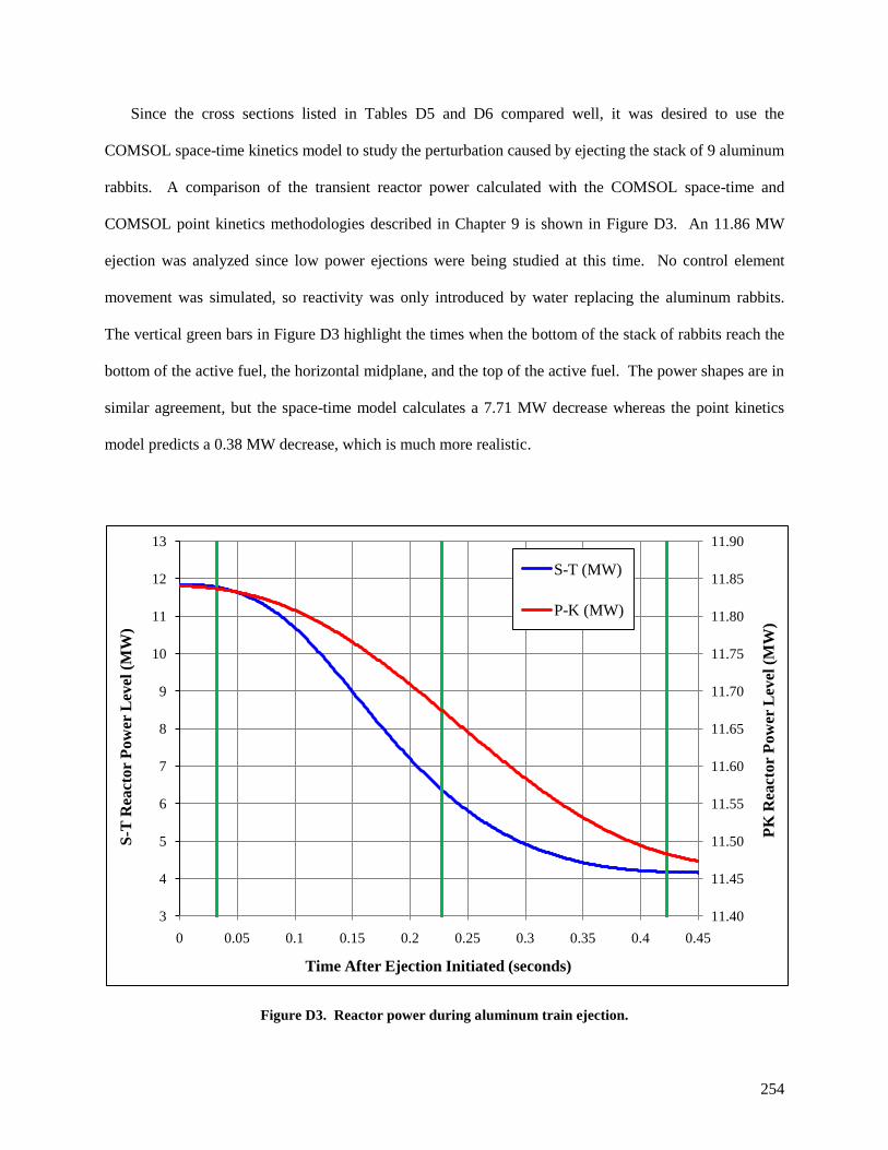
254
Since the cross sections listed in Tables D5 and D6 compared well, it was desired to use the
COMSOL space-time kinetics model to study the perturbation caused by ejecting the stack of 9 aluminum
rabbits. A comparison of the transient reactor power calculated with the COMSOL space-time and
COMSOL point kinetics methodologies described in Chapter 9 is shown in Figure D3. An 11.86 MW
ejection was analyzed since low power ejections were being studied at this time. No control element
movement was simulated, so reactivity was only introduced by water replacing the aluminum rabbits.
The vertical green bars in Figure D3 highlight the times when the bottom of the stack of rabbits reach the
bottom of the active fuel, the horizontal midplane, and the top of the active fuel. The power shapes are in
similar agreement, but the space-time model calculates a 7.71 MW decrease whereas the point kinetics
model predicts a 0.38 MW decrease, which is much more realistic.
Figure D3. Reactor power during aluminum train ejection.
11.40
11.45
11.50
11.55
11.60
11.65
11.70
11.75
11.80
11.85
11.90
3
4
5
6
7
8
9
10
11
12
13
0 0.05 0.1 0.15 0.2 0.25 0.3 0.35 0.4 0.45
PK
Rea
ctor
Pow
er L
evel
(M
W)
S-T
Rea
ctor
Pow
er L
evel
(M
W)
Time After Ejection Initiated (seconds)
S-T (MW)
P-K (MW)

255
The NEWT code performs 2-D (x-y plane) neutron transport calculations, and thus, the geometry of
the HFIR as modeled in the code used to calculate the spatial flux distribution and prepare few-group
cross sections is 2-D. A 2-D model assumes that the geometry is infinitely elongated in the z-direction,
and therefore, the model is per unit depth (z), the properties must be independent of z, and any differential
equation involving the derivative of z can be set to zero. A symmetric boundary condition is used at the
axial centerline where the hydraulic tube is modeled and the largest thermal neutron flux and flux
gradients exist. The hydraulic tube is therefore modeled as if it were infinitely elongated in the z-
direction in the 2-D NEWT model, but in reality, the hydraulic tube is a finite cylinder. This modeling
assumption can cause some issues since HFIR is cylindrical in geometry and the nuclear data being
calculated in 2-D is being used in a 2-D axisymmetric model.
A 2-D axisymmetric (r, z) model has cylindrical geometry (r, z, ϕ) and utilizes symmetry about an
axis of revolution (r = 0). The geometry is defined as a cross section that rotates 360 degrees about the
axis of revolution, which in the black rabbit ejection model is the center of the hydraulic tube. The 3-D
problem is confined to the r-z plane and the circumferential dimension (ϕ) conceptually disappears, the
model is per ―loop length‖ = 2πr, the properties must be independent of ϕ, and any differential equations
involving the derivatives of ϕ can be set to zero. A schematic representation showing the differences
between a 2-D and a 2-D axisymmetric geometry is depicted in Figure D4. The planes outlined by the
blue lines in this illustration represent the r-z plane modeled in COMSOL and the x-y plane modeled in
NEWT.

256
Figure D4. 2-D axisymmetric (left) and 2-D (right) geometry illustrations.
In conclusion, the space-time black rabbit ejection model is over-predicting the effects (transient
reactor power level, reactivity worth, etc.) caused by ejecting the black rabbit out of the HFIR hydraulic
tube. Some investigative studies were performed and documented in this appendix. A summary of the
conclusions are described below:
The few-group nuclear data being calculated via the NEWT representation is not sufficiently
accurate.
o The geometric representation in NEWT appears to provide an inadequate representation of
HFIR geometry. NEWT utilizes 2-D (x, y) geometry, but HFIR is cylindrical (r, z, ϕ).
o The worth of the black rabbit configuration with respect to a water filled hydraulic tube as
calculated by NEWT is 4 times greater than the measured worth.
o The thermal absorption cross section calculated by NEWT is an order of magnitude greater
than that calculated by MCNP.

257
The COMSOL three-group diffusion theory model has a limited area of applicability.
o The power distribution with the black rabbit hydraulic tube configuration does not agree
well with the MCNP and NEWT generated power distributions.
o The worth of the black rabbit configuration is being over-predicted and the neutron fluxes
in the Gd cylinder are being under-predicted in comparison to the MCNP calculation.
o The ejection velocity of the stack of rabbits is approximately 140 cm/s, and thus, the
neutron flux is rapidly varying in time.
The time rate of change in the neutron flux should be small during the time it takes a
neutron to travel a few mean free paths [114].
o Gd has a very large thermal neutron absorption cross section, and thus, is a highly
absorbing media.
The neutron flux should not be rapidly varying, but it is rapidly changing in the
highly absorbing media. Fick’s law applies to systems in which Σs >> Σs, but the Gd
absorption cross section is greater than the Gd scattering cross section.
Table D6. NEWT-derived Gd cross sections.
Cross Section Value (1/cm)
Σa1
3.81E-03
Σa2 5.61E-01
Σa3 9.84E+02
Σs1→2
3.58E-03
Σs1→3
1.43E-10
Σs2→3
4.13E-04
Σs3→2
9.67E-05
The absorption properties change drastically at the Gd/Al interfaces since Al has low
absorption cross sections.

258
VITA
David Chandler was born on January 27, 1985 in West Carrollton, Ohio, to his parents Len and Sheila
Chandler. He is the younger brother and brother-in-law of Louise and Jason Pence. David attended West
Carrollton High School and graduated in May of 2003 as one of his class’ valedictorians and as a scholar
all American soccer player. After graduation, David attended the University of Cincinnati where he
obtained his Bachelors of Science degree in Mechanical Engineering and his Masters of Science degree in
Nuclear Engineering in June and September of 2008, respectively. During his studies at the University of
Cincinnati he worked two quarters as a cooperative education student at Feintool in Blue Ash, OH and
four quarters at Westinghouse Electric Company in Pittsburgh, PA. David performed his M.S. research
as an intern at the Oak Ridge National Laboratory’s High Flux Isotope Reactor in Oak Ridge, TN.
After graduating from the University of Cincinnati, David enrolled at the University of Tennessee and
continued his research at the High Flux Isotope Reactor under the guidance of his advising professor, Dr.
G. Ivan Maldonado, and his technical mentor, Mr. R. Trent Primm, III. David’s Ph. D research interests
are in the field of nuclear reactor physics with an emphasis in Monte Carlo methods, fuel depletion, and
spatially-dependent reactor kinetics. En route to his Ph. D in Nuclear Engineering at the University of
Tennessee, David earned a certificate in nuclear criticality safety. David will graduate with his Ph. D in
the summer of 2011. The next step in David’s life will be to find a fulltime career in Nuclear
Engineering.