lable at ScienceDirect

Atmospheric Environment 155 (2017) 129e139

Contents lists avai

Atmospheric Environment

journal homepage: www.elsevier .com/locate/atmosenv

Spatiotemporal prediction of continuous daily PM2.5 concentrationsacross China using a spatially explicit machine learning algorithm

Yu Zhan a, Yuzhou Luo b, Xunfei Deng c, Huajin Chen b, Michael L. Grieneisen b,Xueyou Shen a, Lizhong Zhu a, *, Minghua Zhang b, **

a Department of Environmental Science, Zhejiang University, Hangzhou, Zhejiang 310058, Chinab Department of Land, Air, and Water Resources, University of California, Davis, CA 95616, USAc Institute of Digital Agriculture, Zhejiang Academy of Agricultural Sciences, Hangzhou, Zhejiang 310021, China

h i g h l i g h t s

* Corresponding author.** Corresponding author.

E-mail addresses: zlz@zju.edu.cn (L. Zhu), mhzhan

http://dx.doi.org/10.1016/j.atmosenv.2017.02.0231352-2310/© 2017 Elsevier Ltd. All rights reserved.

g r a p h i c a l a b s t r a c t

� A novel machine learning model forpredicting daily PM2.5 concentrationsin China.

� This model shows superior predictiveperformance and is able to handlemissing data.

� >90% of the population lived in areaswith annual mean PM2.5 > 35 mg/m3

� >40% of the population was exposedto PM2.5 >75 mg/m3 for over 100 daysin a year.

a r t i c l e i n f o

Article history:Received 16 December 2016Received in revised form8 February 2017Accepted 10 February 2017Available online 15 February 2017

Keywords:Fine particulate matterHuman exposureSpatial nonstationarityGeographically weightedMachine learning

a b s t r a c t

A high degree of uncertainty associated with the emission inventory for China tends to degrade theperformance of chemical transport models in predicting PM2.5 concentrations especially on a daily basis.In this study a novel machine learning algorithm, Geographically-Weighted Gradient Boosting Machine(GW-GBM), was developed by improving GBM through building spatial smoothing kernels to weigh theloss function. This modification addressed the spatial nonstationarity of the relationships between PM2.5

concentrations and predictor variables such as aerosol optical depth (AOD) and meteorological condi-tions. GW-GBM also overcame the estimation bias of PM2.5 concentrations due to missing AOD retrievals,and thus potentially improved subsequent exposure analyses. GW-GBM showed good performance inpredicting daily PM2.5 concentrations (R2 ¼ 0.76, RMSE ¼ 23.0 mg/m3) even with partially missing AODdata, which was better than the original GBM model (R2 ¼ 0.71, RMSE ¼ 25.3 mg/m3). On the basis of thecontinuous spatiotemporal prediction of PM2.5 concentrations, it was predicted that 95% of the popu-lation lived in areas where the estimated annual mean PM2.5 concentration was higher than 35 mg/m3,and 45% of the population was exposed to PM2.5 >75 mg/m3 for over 100 days in 2014. GW-GBMaccurately predicted continuous daily PM2.5 concentrations in China for assessing acute human healtheffects.

© 2017 Elsevier Ltd. All rights reserved.

g@ucdavis.edu (M. Zhang).

1. Introduction

Exposure to fine particulate matter with diameter <2.5 mm(PM2.5) has been associated with increased cardiovascular

Y. Zhan et al. / Atmospheric Environment 155 (2017) 129e139130

morbidity and respiratory mortality (Dockery et al., 1993; Kelleret al., 2015; Madaniyazi et al., 2015; Pope et al., 2011; Puett et al.,2009), as well as decreased birth weight (Rich et al., 2015).Annual average daily PM2.5 exposure levels have been used todevelop exposure-response functions (Burnett et al., 2014), and toassess the Global Burden of Disease or mortality attributable toambient PM2.5 (Apte et al., 2015; Brauer et al., 2012). In addition,reliable daily PM2.5 exposure levels are needed to assess acutehealth effects (Shang et al., 2013), such as acute lower respiratoryinfection for children. China is one of the countries with the mostsevere air pollution by PM2.5 (Brauer et al., 2016; Lai et al., 2013).Severe PM2.5 pollution has attracted public attention, and theChinese government has been implementing regulations whichaim to achieve a 15e25% decrease of PM2.5 concentrations from2012 to 2017 for highly polluted areas (SCPRC, 2013). While the airquality monitoring network has covered most major cities in China(MEPC, 2015), nationwide spatiotemporal distributions of PM2.5concentrations should be delineated for human exposure assess-ment and policy making.

Various models have been developed for predicting thespatiotemporal distributions of PM2.5 concentrations, includingchemical transport models (CTMs) and statistical models.

On the basis of meteorological fields generated by climatemodels, CTMs simulate main processes of chemicals in the atmo-sphere, including emissions, chemistry, transport, and deposition(Jacob, 1999). For instance, the Goddard Earth Observing System-chemical transport (GEOS-Chem) model (Bey et al., 2001), is ableto predict compositions and concentrations of PM2.5 based on thecorresponding emission inventories and environmental conditions(Geng et al., 2015; van Donkelaar et al., 2016). This model is espe-cially valuable for regions without PM2.5 monitoring data, wherestatistical models are generally inapplicable. This model showedgood predictive performance when assimilated with satellite-retrieved aerosol optical depth (AOD), and even better perfor-mance when ground-based PM2.5 observations were also incorpo-rated (van Donkelaar et al., 2016). Nevertheless, CTM's performancecould be undermined by high uncertainty in the emission in-ventories presented on a fine spatiotemporal resolution (e.g.,1� � 1� grids and daily). This is especially true for China, where theamount of annual coal consumption has been corrected up to 12%higher than previously reported (NBSC, 2013; 2015).

Given the established monitoring network in China, sophisti-cated statistical models that do not rely on the emission inventoriestend to be more suitable for predicting spatiotemporal distribu-tions of PM2.5 concentrations in China on a fine spatiotemporalresolution. A number of statistical models, such as the geographi-cally weighted regression (GWR) model (Ma et al., 2014), themixed-effect models (Ma et al., 2016a; Xie et al., 2015), and theBayesian hierarchical model (Lv et al., 2016), have been adopted topredict the PM2.5 concentrations in China. These statistical modelspredict spatiotemporal distributions of PM2.5 based on the ground-based PM2.5 observations, AOD satellite retrievals, meteorologicalconditions, and/or land use types. In dealing with missing data,these statistical models generally employ interpolation to fillmissing AOD retrievals or simply exclude the data points (i.e., datarecords) with missing values (Kloog et al., 2011; Lv et al., 2016; Maet al., 2016a). The exclusion however tends to result in biased es-timates of PM2.5 concentrations (Geng et al., 2015; van Donkelaaret al., 2010). These biased estimates tend to degrade the associ-ated epidemiological analysis, such as the Global Burden of Disease(Naghavi et al., 2015). Although complete sets of AOD retrievals canbe developed by fusing the data from different satellites or throughinterpolation (Nguyen et al., 2012; Xu et al., 2015), the change-of-support problem (i.e., inconsistent spatial units) or the propaga-tion of uncertainty in interpolation are likely to emerge. In addition,

these statistical models that belong to the data modeling cultureassume that the observations are generated by specified stochasticmodels (Breiman, 2001). Nevertheless, the specified models arelikely to oversimplify the otherwise complex relationships betweenPM2.5 concentrations and the predictor variables (Reid et al., 2015),such as by ignoring effects of interaction between predictor vari-ables on PM2.5 or nonlinear relationships between predictor vari-ables and PM2.5.

Machine learning algorithms or models, which pertain to thealgorithmic modeling culture, learn model structures from trainingdata and generally show better predictive performance than con-ventional statistical models (Breiman, 2001; Hastie et al., 2009). Forinstance, a neural network model with a good performance wasdeveloped to predict the daily PM2.5 concentrations in the conti-nental United States (Di et al., 2016). A gradient boosting machine(GBM) model outperformed ten other statistical models in pre-dicting the PM2.5 concentrations in California after a major fireevent (Reid et al., 2015). A GBM model, with the strengths of clas-sification/regression trees and boosting, grows an ensemble ofweak decision trees in a forward and stage-wise fashion (Friedman,2001, 2002). By learning from training data, GBMmodels are able tocapture interaction and nonlinearity in dependence structures, aswell as to handle missing data in a data point, such as missing AODretrieval. However, a “global”model is unable to address the spatialnonstationarity in the relationship between PM2.5 concentrationsand predictor variables. Moreover, trend-fitting methods such asspline interpolation or Kriging are inadequate to capture complexspatial variation (Brunsdon et al., 1996). Thus, the model structureshould alter geographically to reflect the spatial nonstationarity.

This study aims to develop a spatially explicit GBM model,named Geographically Weighted (GW) GBM, for predicting thecontinuous daily PM2.5 concentrations across China. Spatialsmoothing kernels were adopted to model the spatial non-stationarity in the relationship between PM2.5 concentrations andpredictor variables. The GW-GBM model was used to predict thedaily PM2.5 concentrations for 2014 in China (0.5� � 0.5� grids wereused due to the high computational expense of the GW-GBMmodel) based on the ground-based PM2.5 observations, AOD datafrom the Aqua-retrieved Collection 6 of Moderate-resolution Im-aging Spectroradiometer (MODIS) aerosol products (Levy et al.,2013), and meteorological conditions. The predictive performanceof the GW-GBMmodel was evaluated by using cross-validation. Wethen evaluated the estimation bias of PM2.5 concentrations due tomissing AOD retrievals, as well as the interaction, nonlinearity, andspatial nonstationarity of the dependence structure of PM2.5 on thepredictor variables. The GW-GBM model with good predictiveperformance and capable of dealing with missing data is expectedto advance the PM2.5 modeling.

2. Materials and methods

2.1. Data preparation

The GW-GBM model was used to predict the daily PM2.5 con-centrations in 2014 at 0.5� � 0.5� spatial resolution for China (4 194grid cells) based on the ground-based PM2.5 monitoring data(Fig. S1), day of year (DOY), AOD, and meteorological conditions.The PM2.5 monitoring data were retrieved from the National AirQuality Monitoring Network for mainland China and Hainan Island(MEPC, 2015), the Environmental Protection Department of HongKong (http://www.epd.gov.hk) for Hong Kong, and the Environ-mental Protection Administration of Taiwan (http://taqm.epa.gov.tw) for Taiwan. The PM2.5 concentrations were measured witheither the tapered element oscillating microbalance technology orthe beta-attenuation method (Zhao et al., 2016). The monitoring

Y. Zhan et al. / Atmospheric Environment 155 (2017) 129e139 131

sites with less than half-year data were excluded from this analysis.The PM2.5 monitoring data for 1 015 sites from 267 cities wereobtained, which were assigned to their enclosing grid cells. Aver-ages were taken for the cells containing multiple monitoring sites,resulting in 285 grid cells with PM2.5 monitoring data.

The AOD data were obtained from the deep blue/dark targetmerged product contained in the Aqua-retrieved Collection 6MODIS aerosol products at level 2 (Levy et al., 2013). Although1 � 1 km2 AOD products were available from the Multi-AngleImplementation of Atmospheric Correction (MAIAC) algorithm(Lyapustin et al., 2011), these AOD products were not completed forChina in 2014 at the time of this study. The AOD data wereresampled to the delineated grids by averaging. The overall per-centage of missing AOD was 39.1% (Table S1). The daily meteoro-logical conditions, including air temperature, atmosphericpressure, evaporation, precipitation, relative humidity, sunshineduration, and wind speed, for 839 meteorological stations weredownloaded from the China Meteorological Data Center (http://data.cma.cn). The elevation data, with a resolution of 90 m at theequator, were obtained from the Shuttle Radar Topography Mission(SRTM) database (Jarvis et al., 2008). These site-specific meteoro-logical data were interpolated to the delineated grids using co-Kriging with normal score transformation (Deutsch and Journel,1998), where elevation data were incorporated into the estimator.The gridded population density data, with a resolution of 1 km,were obtained from the Data Center for Resources and Environ-mental Sciences for calculating population-weighted PM2.5 con-centrations (RESDC, 2014), which were resampled to the delineatedgrids by averaging. Note that all data were summarized in thedelineated grids used for model development, evaluation, andprediction.

2.2. Model description

The GW-GBM model was developed as an ensemble of GBMmodels, where a single GBM model, hereafter referred to as a sub-model, was used for each predicting cell at 0.5� � 0.5� resolution.Each GW-GBM sub-model was trained to optimize a weightedsquared error loss function for the associated training cells(Ridgeway, 2015):

Lðy; f ðxÞÞ ¼XMm¼1

XNm

n¼1

wm½ymn � f ðxmnÞ�2, XM

m¼1

ðwmNmÞ (1)

where L(y, f(x)) is the loss function for predicting observation y (i.e.,PM2.5 concentrations) by model f(x); x represents predictor vari-ables, including DOY, AOD, atmospheric pressure, air temperature,evaporation, wind speed, relative humidity, sunshine duration, andprecipitation; m is a running index for the training cells (m ¼ 1 toM; M is the total number of training cells, i.e., cells with PM2.5monitoring data); n is a running index for the data points from cellm (n ¼ 1 to Nm; Nm is the total number of data points from cell m);xmn and ymn are values of predictor and response variables,respectively, for data pointmn; andwm is the weight of training cellm, which is determined by the spatial smoothing kernel based onthe distance between this training cell and the predicting cell. Thestrategy for identifying training cells for a targeted predicting cell,as well as the formulas for three commonly adopted spatialsmoothing kernels (i.e., Gaussian, bisquare, and tricube), are listedin the Supplement S2.

The loss function (Eq. (1)) was optimized through the GBMprocedure (Friedman, 2001, 2002). Please see Supplement S1 formore reader-friendly explanations of the following steps.

Initialization : f0ðxÞ ¼XMm¼1

XNm

n¼1

ðwmymnÞ, XM

m¼1

ðwmNmÞ (2)

For k ¼ 1 to K:

Subsampling : fjgS1 ¼ sample�

figNT1 ; S

�(3)

Updating residuals : ~yj ¼ yj � fk�1�xj�

(4)

Growing a tree : fRlkgL1 ¼ tree�n

~yj; xjoS

1

�(5)

Computing terminal node prediction : rlk

¼X

xj2Rlk

�wj~yj

�, Xxj2Rlk

wj (6)

Shrinking the new tree and adding it to the model:

fkðxÞ ¼ fk�1ðxÞ þ lrlkIðx2RlkÞ (7)

where at each step k, a subsample with S data points fjgS1 are drawn

from the training dataset figNT1 at random without replacement

(NT ¼ PMm¼1Nm); ~yj is the pseudo residual produced by the model

updated at the previous step annotated as fk-1(xj); Rlk represents theregion of the predictor feature space corresponding to terminal l ofthe new tree with L terminals; rlk is the prediction for terminal l;wj

is the weight of the cell that contains data point j; and l is theshrinkage rate (l ¼ 0.05). In growing a tree (step 5), it starts with asingle (root) node, and then searches over all binary splits of allpredictor variables for the one that reduces the weighted squarederror loss the most. The tree-split process iterates until the mini-mum number of data points in a terminal node (default: 10) or themaximum tree depth is reached. The tree depth (i.e., interactiondepth) is the length of the longest path from the root to the ter-minal nodes, which reflects the interaction among the predictorvariables. For example, a tree depth of 1 implies an additive model,and a depth of 2 implies 2-way interactions.

Note that K is determined with sample-based 10-fold cross-validation, where the training samples are randomly partitionedinto 10 groups of approximately the same size (Elith et al., 2008).Starting with a selected K’ (e.g., 50), the GW-GBM model trainedwith 9 groups makes predictions for the remaining group, which isrepeated 10 times to obtain a complete set of predictions, and theroot-mean-square error (RMSE) is recorded. This process isrepeated with a larger K0 until the RMSE does not decrease for 5steps. K is set to the optimal K’ and is used to train the formal GW-GBM model.

2.3. Missing data handling

As a tree-based model, the GW-GBM model can handle missingdata for continuous predictor variables by using surrogate splits(Breiman et al., 1984). In growing trees, primary splits were firstdetermined by using the subset of data with complete records foreach partially missing variable. Then, a list of surrogate predictorvariables and split points (namely surrogate splits) were formed,which produce splits similar to the primary splits. When makingpredictions based on the data points with missing records of agiven variable, the surrogate splits were chosen in the order of their

Y. Zhan et al. / Atmospheric Environment 155 (2017) 129e139132

similarity to the primary splits in case some surrogate splits are stillunavailable due to missing data.

2.4. Model prediction

The continuous daily PM2.5 concentrations for China in 2014were predicted on the 0.5� � 0.5� grids using the GW-GBM model.Seven regions of China were used for spatially summarizing modelpredictions, including North, Northwest, Northeast, East, Central,South, and Southwest China (Fig. S1). The annual and quarterlyaverages of PM2.5 concentrations were summarized from the pre-dicted daily concentrations. For human exposure assessment,population-weighted PM2.5 concentrations were calculated on thenational and regional levels (van Donkelaar et al., 2015).

PPW ¼XNi¼1

ðPi � CiÞ,XN

i¼1

Pi (8)

where PPW is the population-weighted PM2.5 concentration for aregion covering N grid cells; Pi is the population density of grid celli; and Ci is the PM2.5 concentration of grid cell i. The short- andlong-term PM2.5 exposure levels for the population in China wereevaluated.

Table 1Predictive performance based on datasets excluding or including the data pointswith missing AOD values in cross-validation.

Excluding missing AODa Including missing AODb

GW-GBM Original GBM GW-GBM Original GBM

RMSE (mg/m3) 24.3 25.5 23.0 25.3R2 0.74 0.71 0.76 0.71Slope 0.75 0.72 0.77 0.71

a Summary of the monitoring PM2.5: 62.9 ± 47.6 mg/m3 (m±s; n ¼ 37 626).b Summary of the monitoring PM2.5: 58.2 ± 47.2 mg/m3 (m±s; n ¼ 103071).

2.5. Model evaluation

The GW-GBM model was evaluated with cell-based 10-foldcross-validation, where the training cells were randomly parti-tioned into 10 groups of approximately the same size. The subse-quent steps for obtaining the predictions were similar to those ofsample-based 10-fold cross-validation mentioned in the “ModelDescription” section, i.e., the GW-GBMmodel trainedwith 9 groupsmade predictions for the remaining group, which was repeated 10times to obtain a complete set of predictions. Note that in themodelevaluation, the sample-based cross-validation to determine K wasconducted for each repeat of the cell-based cross-validation. Toshow the improvement by integrating the geographically weightedmethod, a regular GBM model (hereafter referred to as the originalGBM model) was also developed and evaluated with the sametraining dataset. The predictive performances were measured withthe root-mean-square error (RMSE) and coefficient of determina-tion (R2) in the cross-validation.

In order to test the effectiveness of surrogate splits for handlingpartially missing data in the GW-GBM model, the quarterly andannual averages of PM2.5 predictions for all simulation days werecompared with those excluding days with missing AOD data. Thedifferences were plotted in maps, and considered as potentialestimation bias if the missing AOD data could not be handled by amodel.

The spatial variation of the importance of predictor variables forpredicting PM2.5 concentrations was evaluated. Here the impor-tance of a predictor variable was defined based on the number oftimes the variable was used for tree splitting and the consequenterror reduction in each GW-GBM sub-model (Friedman, 2001). Theformulas for the variable importance measures are listed in theSupplement S3. For each sub-model (or predicting cell), theimportance measures of all predictor variables were scaled so thattheir sum was equal to 100 for more intuitive interpretation. Theoverall importance measures of the GW-GBM model were calcu-lated as the averages over all cells. The GW-GBM model wasimplemented in R by mainly adapting from package gbm (RDevelopment Core Team, 2015; Ridgeway, 2015).

3. Results

3.1. Predictive performance

On the basis of the cross-validation results (Table 1), the GW-GBM model showed good performance in predicting daily PM2.5concentrations even when AOD data were partially missing(R2 ¼ 0.76, RMSE¼ 23.0 mg/m3), which was better than the originalGBM model (R2 ¼ 0.71, RMSE ¼ 25.3 mg/m3). The R2 by region andseason ranged from 0.21 for the third quarter in Northwest China(due to the relative small number of monitoring sites in that region;Fig. S1) to 0.79 for the first quarter in East China (Table S2). Theperformance of the GW-GBM model was generally not sensitive tothe spatial smoothing kernel types (Table S3), although the bis-quare kernel showed slightly better performance than the tricubeand Gaussian kernels. Compared to the statistical measures basedon daily data, the GW-GBM model showed better performance forPM2.5 predictions on monthly, quarterly, and annual levels, with R2

of 0.84, 0.85, and 0.84, respectively (Fig. 1).

3.2. Spatiotemporal distributions of PM2.5 concentrations

As annual population-weighted averages by region (refer toFig. S1 for the locations of these regions), the highest PM2.5 con-centrations in 2014 were predicted in North China (77.5 mg/m3),followed by Central China (71.5 mg/m3) (Table 2). These two regionsare highly populated with 39.2% of the total population of China.South China consistently showed the lowest PM2.5 levels across theyear. Seasonally, the highest national average PM2.5 concentrationswere predicted in the first quarter (86.0 mg/m3), and the lowest inthe third quarter (40.1 mg/m3). In the Central and North China, theaverage daily PM2.5 were predicted to be > 100 mg/m3 during thefirst quarter. PM2.5 pollution was much alleviated in the thirdquarter for most of China, except for the southeast region of NorthChina (including the national capital region of Beijing-Tianjin-Hebei) and deserts in Northwest China (Fig. 2). The predictedspatiotemporal distributions of PM2.5 concentrations were gener-ally consistent with the previous studies for China in 2014 (Youet al., 2016a, 2016b), though those two studies did not reportpopulation-weighted PM2.5 concentrations.

3.3. Exposure to ambient PM2.5

On the basis of the continuous spatiotemporal prediction ofPM2.5 concentrations, it was found that 95% of the Chinese popu-lation in 2014 lived in areas where the estimated annual meanPM2.5 concentrationwas >35 mg/m3, and 45% of the populationwasexposed to PM2.5>75 mg/m3 for more than 100 days (Fig. 3). Thelevels of 35 and 75 mg/m3 are based on World Health Organization(WHO)’s annual and 24-h mean interim target 1 (IT1) air qualityguidelines, respectively (WHO, 2006). Spatially, South China hadthe highest percent of population (26%) living in areas meeting theannual IT1, while the lowest levels were in Northeast and Central

Fig. 1. Evaluation of the predictive performance of the GW-GBM model by using cross-validation at (A) daily, (B) monthly, (C) quarterly, and (D) annual levels.

Table 2Quarterly and annual averages ± standard deviations of population weighted PM2.5 concentrations for each region and the whole nation of China in 2014 (mg/m3).

Regiona Q1b Q2 Q3 Q4 Annual

Central China 103.2 ± 42.9 62.7 ± 15.0 45.2 ± 10.8 75.4 ± 23.7 71.5 ± 33.5East China 80.4 ± 39.3 59.9 ± 17.3 41.4 ± 11.8 61.9 ± 19.5 60.8 ± 27.8North China 106.3 ± 46.2 62.4 ± 18.3 55.2 ± 14.0 86.5 ± 37.7 77.5 ± 37.6Northeast China 75.0 ± 30.8 39.5 ± 12.9 35.9 ± 15.0 75.3 ± 37.3 56.4 ± 32.1Northwest China 86.4 ± 27.9 52.4 ± 15.8 38.4 ± 7.0 62.5 ± 16.2 59.8 ± 25.2South China 54.6 ± 24.6 31.1 ± 8.9 24.3 ± 6.5 48.1 ± 12.2 39.5 ± 19.1Southwest China 83.4 ± 33.0 47.4 ± 9.9 33.2 ± 6.5 57.4 ± 17.2 55.2 ± 26.7Nation 86.0 ± 29.0 52.2 ± 8.7 40.1 ± 6.7 68.1 ± 16.9 61.6 ± 24.5

a Regions are labelled on Fig. S1.b Q1: JanuaryeMarch; Q2: AprileJune; Q3: JulyeSeptember; Q4: OctobereDecember.

Y. Zhan et al. / Atmospheric Environment 155 (2017) 129e139 133

China (both are 0%). In addition, 33% of the Chinese populationwasexposed to annual mean PM2.5 >70 mg/m3 (twice of the annual IT1).Moreover, Fig. 3B shows the two-way cumulative distributions ofPM2.5 exposure intensity and duration at the daily level. Not onlywas the majority of the population exposed to PM2.5 exceeding thedaily IT1 for most days of the year, but many were also exposed toeven higher PM2.5 for at least a few days in a year. For instance, 55%of the national population was exposed to PM2.5 >150 mg/m3 formore than 10 days in 2014. Note that the personal exposure wouldlikely be more variable than the exposure predicted in this studydue to the use of grid-cell PM2.5 averages. The personal exposurewould be affected by the personal activity pattern, indoor-outdoorair exchange rate, and spatial heterogeneity within each grid cell.

3.4. Estimation bias due to missing AOD retrievals

To evaluate the improvement of model performance withmissing data handling, two sets of annual and quarterly averages of

PM2.5 concentration were calculated by including and excludingGW-GBM predictions for the data points with missing AOD data,and their differences were compared. Without the missing datahandling implemented in GW-GBM, the average PM2.5 concentra-tions would have been highly underestimated in Northeast China,and overestimated in South, East, and Northwest China (Fig. 4). Themagnitudes of the differences in average PM2.5 predictions gener-ally followed the spatiotemporal distributions of the missing rate ofAOD coverage (Fig. S2). Higher absolute values of the differenceswere associated with lower AOD coverage rates. Without missingdata handling by GW-GBM model, reduced average PM2.5 concen-trations (reduced by up to 50 mg/m3) would be reported inNortheast China, especially during the first and fourth quarterswhen the AOD coverage rates were lower than 20% for a large partof that region. Similarly, the GW-GBM model avoided the potentialoverestimation (up to >50 mg/m3) of PM2.5 concentrations due toAOD data missing in the first and second quarters for South andEast China, and in the second quarter for Northwest China (Fig. 4).

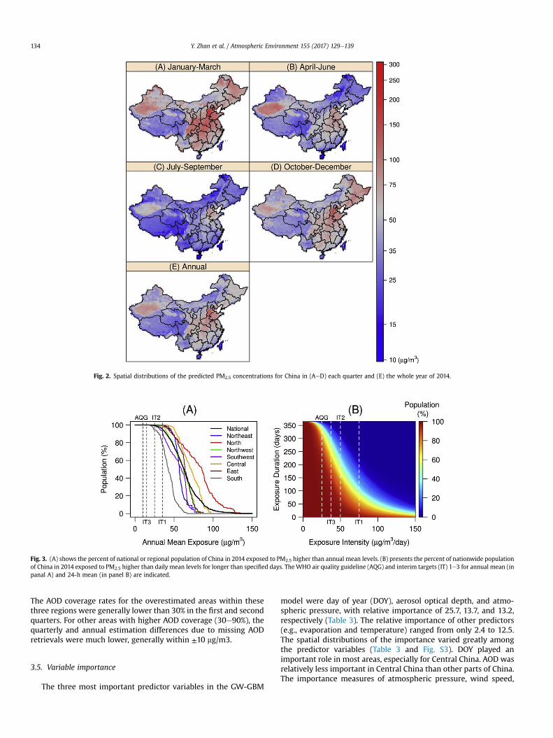
Fig. 2. Spatial distributions of the predicted PM2.5 concentrations for China in (AeD) each quarter and (E) the whole year of 2014.

Fig. 3. (A) shows the percent of national or regional population of China in 2014 exposed to PM2.5 higher than annual mean levels. (B) presents the percent of nationwide populationof China in 2014 exposed to PM2.5 higher than daily mean levels for longer than specified days. The WHO air quality guideline (AQG) and interim targets (IT) 1e3 for annual mean (inpanal A) and 24-h mean (in panel B) are indicated.

Y. Zhan et al. / Atmospheric Environment 155 (2017) 129e139134

The AOD coverage rates for the overestimated areas within thesethree regions were generally lower than 30% in the first and secondquarters. For other areas with higher AOD coverage (30e90%), thequarterly and annual estimation differences due to missing AODretrievals were much lower, generally within ±10 mg/m3.

3.5. Variable importance

The three most important predictor variables in the GW-GBM

model were day of year (DOY), aerosol optical depth, and atmo-spheric pressure, with relative importance of 25.7, 13.7, and 13.2,respectively (Table 3). The relative importance of other predictors(e.g., evaporation and temperature) ranged from only 2.4 to 12.5.The spatial distributions of the importance varied greatly amongthe predictor variables (Table 3 and Fig. S3). DOY played animportant role in most areas, especially for Central China. AOD wasrelatively less important in Central China than other parts of China.The importance measures of atmospheric pressure, wind speed,

Fig. 4. Estimation bias of average PM2.5 concentrations due to missing AOD retrievals for (AeD) each quarter and (E) the whole year of 2014 in China. The estimation bias is thedifference between the average of all predicted daily PM2.5 concentrations and the average of those with AOD retrievals. Areas with no AOD retrievals during the study periods arenot included (blank areas within the study domain).

Table 3Average variable importance in the GW-GBM model for each region of China.

Regiona DOYb AOD PRS TEM WIN EVP RHU SSD PRE

Central China 42.6 6.7 9.1 10.0 4.9 8.5 7.6 6.1 4.6East China 36.1 7.3 9.7 12.3 6.1 8.5 7.5 7.8 4.8North China 22.0 12.3 12.4 15.1 8.4 11.7 7.8 8.5 1.8Northeast China 22.8 10.5 7.5 17.5 11.9 11.0 9.7 7.8 1.4Northwest China 22.2 18.2 15.0 12.9 11.0 5.9 6.5 6.9 1.4South China 29.2 8.1 11.1 12.5 10.9 6.6 12.9 5.0 3.9Southwest China 27.7 14.9 16.3 8.4 12.6 6.9 5.4 4.6 3.2Nation 25.7 13.7 13.2 12.5 10.4 8.1 7.4 6.6 2.4

a Regions are labelled on Fig. S1.b Variable acronyms: Day of Year (DOY), Aerosol Optical Depth (AOD), Atmo-

spheric Pressure (PRS), Air Temperature (TEM), Wind Speed (WIN), Evaporation(EVP), Relative Humidity (RHU), Sunshine Duration (SSD), and Precipitation (PRE).Please see Fig. S3 for the detailed spatial distributions of variable importance.

Y. Zhan et al. / Atmospheric Environment 155 (2017) 129e139 135

and sunshine duration were relatively higher in Northwest Chinaand Tibetan Plateau than in other regions. Air temperatureexhibited high importance in Northeast China and a coastal part ofSouth China. The North China Plain (with notoriously severe PM2.5pollution) showed higher importance of evaporation and sunshineduration than other regions. The importance measures of relativehumidity and precipitationwere relatively higher in South and EastChina, respectively.

4. Discussion

The GW-GBM model showed good performance in predicting

continuous spatiotemporal PM2.5 concentrations in China. Ac-cording to the values of R2, the performance of the GW-GBM(R2 ¼ 0.76) was better than a previous national study withR2 ¼ 0.64 (Ma et al., 2014), a regional study in the North China Plainwith R2 ¼ 0.61 using 10-fold leave-10%-cities-out cross-validation(Lv et al., 2016), and other previous studies (Table S4). These studiesemployed artificial neural network, Bayesian hierarchical model,geographically weighted regression, and mixed-effects models. It isworthy to note that, besides the model algorithms and predictorvariables, validation strategies also affected the resulting values ofstatistical measures for model performance. For cross-validation,input data could be partitioned by data points, monitoring sites,or grid cells, which were named as sample-, site-, or cell-basedcross-validation, respectively.

In this study cell-based 10-fold cross-validationwas used, wherethe training cells are partitioned into 10 groups. In another nationalstudy, Ma et al. (2016a) used sample-based cross-validation asindicated in their later study (Ma et al., 2016b), where the samplesof data points were partitioned into 10 groups, and reported ahigher R2 of 0.79. In this study whenmissing-AOD data points wereexcluded (to be comparable with the previous studies), the sample-and site-based cross-validations resulted in much better perfor-mance, according to statistical measures (R2 ¼ 0.88 and 0.87,respectively), than the cell-based cross-validation (R2 ¼ 0.74)(Table S5). This was probably due to higher correlation betweentraining and predicting datasets for the sample-/site-based thanthe cell-based cross-validation. Since the main purpose of themodels was to predict PM2.5 concentrations in unmonitored cells,

Y. Zhan et al. / Atmospheric Environment 155 (2017) 129e139136

the training/predicting data partition of the cell-based cross-vali-dation better reflected the relationship between training and pre-dicting data for real prediction. Moreover, a higher density ofmonitoring sites was available in urban areas, and PM2.5 concen-trations observed within a city were usually similar to each other.Compared to cell-based cross-validation where virtually one“average” site was considered for each cell, site-based cross-vali-dation might lead to over-optimistic estimation of model perfor-mance due to the repeated uses of similar measurements within acell (Lv et al., 2016).

The geographically weightedmethod refined the GBMmodel byexplicitly addressing the spatial nonstationarity of the dependenceof PM2.5 concentrations on predictor variables. It was recognizedthat the relationship between PM2.5 concentrations and AOD wasspatially nonstationary, especially across a large region (Paciorekand Liu, 2009). Also, the spatial nonstationarity was suggested bythe spatial variability on the relative importance of predictor vari-ables across China (Table 3, Fig. S3). The spatial nonstationaritybetween PM2.5 concentrations and AOD was partially addressed bythe meteorological variables. Moreover, the geographicallyweightedmethod implemented smoothing kernels to screen quasi-stationary areas and to smooth transitions between nonstationaryareas. Although the spatial nonstationarity could be addressed byincluding spatial coordinates as predictor variables in the model,apparent artificial strips emerged in the predicted spatial distri-butions of PM2.5 concentrations (Fig. S4). Furthermore, it is alsoimportant to address temporal nonstationarity between PM2.5

concentrations and AOD (Kloog et al., 2011). With sufficientcomputing resources in the future, spatiotemporal smoothingkernels may be implemented in the GW-GBM model to addressspatial and temporal nonstationarity simultaneously. Note that theGW-GBM model consists of an ensemble of GW-GBM sub-models,whose number is proportional to the complexity of smoothingkernels implemented, thus it is much more computationallyexpensive than the original GBM model.

The important predictor variables on the PM2.5 concentrationswere identified, which provided valuable information foradvancing PM2.5 prediction in the future. The seasonality of PM2.5concentrations (DOY) derived from the monitoring data was themost important variable. In general, the PM2.5 concentrations wererelatively low in warm seasons and high in cold seasons, resultingfrom the seasonality of pollutant emissions and meteorologicalconditions. The meteorological variables were also highly impor-tant for predicting PM2.5 concentrations. Air pollutants tended toaccumulate when the atmospheric pressure were high and thewind speed were low, which might be enhanced by surface tem-perature inversion (Zhao et al., 2013). Scavenging by precipitationwas important to removal of PM2.5 (Tai et al., 2010). While AODwascommonly acknowledged as a good indicator of ambient PM2.5, inthis study its importance measure was similar to individual mete-orological variables. Besides the limited availability of AOD data inthe study area (<50% coverage as an annual average), the PM2.5-AOD relationship of high uncertainty also degraded the importanceof AOD (Paciorek and Liu, 2009). This relationship for examplemight be affected by the vertical profile of aerosol. Previous studiesused the vertical profile simulated by CTMs, e.g., GEOS-Chem, as ascaling factor to estimate the proportion of aerosol depth attrib-utable to ground-level PM2.5 (Liu et al., 2004; van Donkelaar et al.,2006). In the future, we also intend to integrate the vertical profileof aerosol into the GW-GBM model for better predictionperformance.

Obvious nonlinear and interaction effects of the predictor vari-ables on the PM2.5 concentrations were revealed by the partialdependence plots and interaction depths, respectively. A partialdependence plot shows the effect of a variable on the response after

accounting for the average effects of all other variables in themodel(Supplement S4). Nonlinearity means a nonlinear relationship be-tween a predictor variable and PM2.5 concentrations. Interaction isused when the effects of multiple predictor variables on PM2.5concentrations are not equal to the sum of their individual effects.In the GBM or GW-GBM model, while a single decision tree cannotproduce nonlinearity, a combination of hundreds or thousands ofshrunken trees can fit a nonlinear function (Eq. (7)). The partialdependence plots of the original GBM model reflect the overallnonlinear relationships of the PM2.5 concentrations with a fewpredictor variables (Fig. S5). For example, the partial dependence ofPM2.5 concentrations on evaporation initially decreased quicklyalong with the increase of evaporation and then leveled off. Inaddition, a GW-GBM model consisting of tree stubs indicated nointeraction effect, and deep tree depth indicated strong interactioneffects. In this study, the complex tree structures (interaction ortree depth: 8.0 ± 2.4) of the fitted GW-GBM model suggest stronginteraction effects between the predictor variables on the PM2.5concentrations. Therefore, additive or linear structures were inad-equate for modelling PM2.5 concentrations.

The GW-GBM model improved the prediction capability forPM2.5 by handling incomplete input data, particularly partiallymissing AOD retrievals. In Northeast China, for example, AOD re-trievals tended to be missing in the first and fourth quarters(Fig. S2), which might be related to high reflectance of snow. At thesame time, high PM2.5 concentrations were also predicted (Table 2).More fuel was combusted for heating in cold days, usually accom-panied with snow cover (Xu et al., 2011), resulting in higher PM2.5concentrations compared to warmer days when AOD retrievalswere available. In contrast, AOD retrievals in South China tended tobemissing in the first and second quarters (Fig. S2), whichmight bedue to cloud cover associated with rain. Compared to sunny days,PM2.5 concentrations in rainy days were lower because of rainscavenging. If a model did not generate PM2.5 predictions for thedata points with missing AOD data during those months (Ma et al.,2016a), it would generate biased estimates of the pollution andexposure level in terms of average concentrations (Fig. 4). Sincemissing AOD data are frequently observed during highly pollutedperiods in China, missing data handling is very important for ac-curate PM2.5 predictions in China.

The GW-GBM model equipped with surrogate splits was supe-rior to traditional statistical models in handling missing data forPM2.5 prediction. Traditional statistical models were generallyincapable of making predictions for the modeling time nodes wheninput data were partially missing. Thus, these models relied onother methods to fill the data gaps. In previous studies, data fusionor interpolation were conducted to fill AOD gaps (Lv et al., 2016;Nguyen et al., 2012; Xu et al., 2015), where AOD were fused frommultiple data sources and/or geostatistical interpolation (e.g.,Kriging) was used to fill the missing values. Another method was tointerpolate PM2.5 values estimated for the data points with AODretrievals to those with missing values through smoothing such asthin plate spline (Kloog et al., 2011). However, change-of-support oruncertainty propagation might emerge as a result, and the inter-polation tended to smooth spatial variations of AOD or PM2.5. Toavoid these problems, the GW-GBM model built surrogate splitsbased on the patterns learned from the training data with AODretrieved from the Aqua satellite only. Surrogate splits utilizedcorrelations of AOD values with the other predictor variables toreduce the loss of information due to missing values (Hastie et al.,2009). As the AOD missing rates were considerable in PM2.5 pre-diction, it was better to use a model that could handle missing datathan to use models that relied on additional missing data fillingmethods.

Y. Zhan et al. / Atmospheric Environment 155 (2017) 129e139 137

5. Conclusions

A spatially explicit machine learning algorithm, named GW-GBM, was developed to predict the spatiotemporal distributionsof continuous daily PM2.5 concentrations in China. All predictorvariables of the model are readily available from public data sour-ces. The GW-GBM model addressed spatial nonstationarity of thedependence of PM2.5 on environmental conditions, considerablyimproving the predictive performance. The GW-GBM modelrevealed interaction and nonlinear effects that are underrepre-sented by conventional statistical models. The GW-GBMmodel alsoovercame the estimation bias of PM2.5 concentrations due tomissing AOD retrievals, which tends to bias the exposure analyses.This study provided reliable data, such as exposure intensity andduration, for assessing acute human health effects of PM2.5 expo-sure in China. In the future, comparative analyses with epidemio-logical data in China are expected to provide helpful information forrefining exposure-response curves at higher PM2.5 concentrations.

Acknowledgements

This work was supported by the National Natural ScienceFoundation of China [21607127], and the Key Research and Devel-opment Program of Ministry of Science and Technology of China[2016YFC020710].

Appendix A. Supplementary data

Supplementary data related to this article can be found at http://dx.doi.org/10.1016/j.atmosenv.2017.02.023.

References

Apte, J.S., Marshall, J.D., Cohen, A.J., Brauer, M., 2015. Addressing global mortalityfrom ambient PM2.5. Environ. Sci. Technol. 49, 8057e8066.

Bey, I., Jacob, D.J., Yantosca, R.M., Logan, J.A., Field, B.D., Fiore, A.M., Li, Q., Liu, H.Y.,Mickley, L.J., Schultz, M.G., 2001. Global modeling of tropospheric chemistrywith assimilated meteorology: model description and evaluation. J. Geophys.Res. Atmos. 106, 23073e23095.

Brauer, M., Amann, M., Burnett, R.T., Cohen, A., Dentener, F., Ezzati, M.,Henderson, S.B., Krzyzanowski, M., Martin, R.V., Van Dingenen, R., vanDonkelaar, A., Thurston, G.D., 2012. Exposure assessment for estimation of theGlobal Burden of Disease attributable to outdoor air pollution. Environ. Sci.Technol. 46, 652e660.

Brauer, M., Freedman, G., Frostad, J., van Donkelaar, A., Martin, R.V., Dentener, F.,Dingenen, R.v., Estep, K., Amini, H., Apte, J.S., Balakrishnan, K., Barregard, L.,Broday, D., Feigin, V., Ghosh, S., Hopke, P.K., Knibbs, L.D., Kokubo, Y., Liu, Y.,Ma, S., Morawska, L., Sangrador, J.L.T., Shaddick, G., Anderson, H.R., Vos, T.,Forouzanfar, M.H., Burnett, R.T., Cohen, A., 2016. Ambient air pollution exposureestimation for the Global Burden of Disease 2013. Environ. Sci. Technol. 50,79e88.

Breiman, L., 2001. Statistical modeling: the two cultures. Stat. Sci. 16, 199e215.Breiman, L., Friedman, J., Stone, C.J., Olshen, R.A., 1984. Classification and Regression

Trees. ed eds. New York: Wadsworth.Brunsdon, C., Fotheringham, A.S., Charlton, M.E., 1996. Geographically weighted

regression: a method for exploring spatial nonstationarity. Geogr. Anal. 28,281e298.

Burnett, R.T., Pope 3rd, C.A., Ezzati, M., Olives, C., Lim, S.S., Mehta, S., Shin, H.H.,Singh, G., Hubbell, B., Brauer, M., Anderson, H.R., Smith, K.R., Balmes, J.R.,Bruce, N.G., Kan, H., Laden, F., Pruss-Ustun, A., Turner, M.C., Gapstur, S.M.,Diver, W.R., Cohen, A., 2014. An integrated risk function for estimating theglobal burden of disease attributable to ambient fine particulate matter expo-sure. Environ. Health Perspect. 122, 397e403.

Deutsch, C.V., Journel, A.G., 1998. GSLIB Geostatistical Software Library and User'sGuide. eds, second ed. Oxford University Press, New York.

Di, Q., Kloog, I., Koutrakis, P., Lyapustin, A., Wang, Y., Schwartz, J., 2016. AssessingPM2.5 exposures with high spatiotemporal resolution across the continentalUnited States. Environ. Sci. Technol. 50, 4712e4721.

Dockery, D.W., Pope, C.A., Xu, X., Spengler, J.D., Ware, J.H., Fay, M.E., Ferris, B.G.J.,Speizer, F.E., 1993. An association between air pollution and mortality in six U.S.cities. N. Engl. J. Med. 329, 1753e1759.

Elith, J., Leathwick, J.R., Hastie, T., 2008. A working guide to boosted regressiontrees. J. Anim. Ecol. 77, 802e813.

Friedman, J.H., 2001. Greedy function approximation: a gradient boosting machine.Ann. Stat. 29, 1189e1232.

Friedman, J.H., 2002. Stochastic gradient boosting. Comput. Stat. Data Anal. 38,367e378.

Geng, G., Zhang, Q., Martin, R.V., van Donkelaar, A., Huo, H., Che, H., Lin, J., He, K.,2015. Estimating long-term PM2.5 concentrations in China using satellite-basedaerosol optical depth and a chemical transport model. Remote Sens. Environ.166, 262e270.

Hastie, T., Tibshirani, R., Friedman, J., 2009. The Elements of Statistical Learning:Data Mining, Inference, and Prediction. eds, second ed. Springer-Verlag, NewYork.

Jacob, D., 1999. Introduction to Atmospheric Chemistry Ed. eds. Princeton Uni-versity Press, Princeton, New Jersey.

Jarvis, A., Reuter, H.I., Nelson, A., Guevara, E., 2008. Hole-filled seamless SRTM dataV4.1. International Centre for Trop.ical Agric.ulture (CIAT). http://srtm.csi.cgiar.org.

Keller, J.P., Olives, C., Kim, S.Y., Sheppard, L., Sampson, P.D., Szpiro, A.A., Oron, A.P.,Lindstrom, J., Vedal, S., Kaufman, J.D., 2015. A unified spatiotemporal modelingapproach for predicting concentrations of multiple air pollutants in the multi-ethnic study of atherosclerosis and air pollution. Environ. Health Perspect. 123,301e309.

Kloog, I., Koutrakis, P., Coull, B.A., Lee, H.J., Schwartz, J., 2011. Assessing temporallyand spatially resolved PM2.5 exposures for epidemiological studies using sat-ellite aerosol optical depth measurements. Atmos. Environ. 45, 6267e6275.

Lai, H.-K., Hedley, A.J., Thach, T.Q., Wong, C.-M., 2013. A method to derive therelationship between the annual and short-term air quality limitsdanalysisusing the WHO Air Quality Guidelines for health protection. Environ. Int. 59,86e91.

Levy, R.C., Mattoo, S., Munchak, L.A., Remer, L.A., Sayer, A.M., Patadia, F., Hsu, N.C.,2013. The Collection 6 MODIS aerosol products over land and ocean. Atmos.Meas. Tech. 6, 2989e3034.

Liu, Y., Park, R.J., Jacob, D.J., Li, Q., Kilaru, V., Sarnat, J.A., 2004. Mapping annual meanground-level PM2.5 concentrations using Multiangle Imaging Spectroradi-ometer aerosol optical thickness over the contiguous United States. J. Geophys.Res. Atmos. 109, 1e10.

Lv, B., Hu, Y., Chang, H.H., Russell, A.G., Bai, Y., 2016. Improving the accuracy of dailyPM2.5 distributions derived from the fusion of ground-level measurements withaerosol optical depth observations, a case study in North China. Environ. Sci.Technol. 50, 4752e4759.

Lyapustin, A., Wang, Y., Laszlo, I., Kahn, R., Korkin, S., Remer, L., Levy, R., Reid, J.S.,2011. Multiangle implementation of atmospheric correction (MAIAC): 2. Aerosolalgorithm. J. Geophys. Res. Atmos. 116.

Ma, Z., Hu, X., Huang, L., Bi, J., Liu, Y., 2014. Estimating ground-level PM2.5 in Chinausing satellite remote sensing. Environ. Sci. Technol. 48, 7436e7444.

Ma, Z., Hu, X., Sayer, A.M., Levy, R., Zhang, Q., Xue, Y., Tong, S., Bi, J., Huang, L., Liu, Y.,2016a. Satellite-based spatiotemporal trends in PM2.5 concentrations: China,2004-2013. Environ. Health Perspect. 124, 184e192.

Ma, Z., Liu, Y., Zhao, Q., Liu, M., Zhou, Y., Bi, J., 2016b. Satellite-derived high reso-lution PM2.5 concentrations in Yangtze River Delta Region of China usingimproved linear mixed effects model. Atmos. Environ. 133, 156e164.

Madaniyazi, L., Nagashima, T., Guo, Y., Yu, W., Tong, S., 2015. Projecting fine par-ticulate matter-related mortality in East China. Environ. Sci. Technol. 49,11141e11150.

MEPC, 2015. Air Quality Daily Report.: Ministry of Environmental Protection of thePeople's Republic of China. http://datacenter.mep.gov.cn/.

Naghavi, M., Wang, H., Lozano, R., Davis, A., Liang, X., Zhou, M., Vollset, S.E.,Ozgoren, A.A., Abdalla, S., Abd-Allah, F., Aziz, M.I.A., Abera, S.F., Aboyans, V.,Abraham, B., Abraham, J.P., Abuabara, K.E., Abubakar, I., Abu-Raddad, L.J., Abu-Rmeileh, N.M.E., Achoki, T., Adelekan, A., Ademi, Z.N., Adofo, K., Adou, A.K.,Adsuar, J.C., Aernlov, J., Agardh, E.E., Akena, D., Al Khabouri, M.J., Alasfoor, D.,Albittar, M., Alegretti, M.A., Aleman, A.V., Alemu, Z.A., Alfonso-Cristancho, R.,Alhabib, S., Ali, M.K., Ali, R., Alla, F., Al Lami, F., Allebeck, P., AlMazroa, M.A.,Salman, R.A.-S., Alsharif, U., Alvarez, E., Alviz-Guzman, N., Amankwaa, A.A.,Amare, A.T., Ameli, O., Amini, H., Ammar, W., Anderson, H.R., Anderson, B.O.,Antonio, C.A.T., Anwari, P., Apfel, H., Cunningham, S.A., Arsenijevic, V.S.A., Al, A.,Asad, M.M., Asghar, R.J., Assadi, R., Atkins, L.S., Atkinson, C., Badawi, A.,Bahit, M.C., Bakfalouni, T., Balakrishnan, K., Balalla, S., Banerjee, A., Barber, R.M.,Barker-Collo, S.L., Barquera, S., Barregard, L., Barrero, L.H., Barrientos-Gutierrez, T., Basu, A., Basu, S., Basulaiman, M.O., Beardsley, J., Bedi, N., Beghi, E.,Bekele, T., Bell, M.L., Benjet, C., Bennett, D.A., Bensenor, I.M., Benzian, H., Ber-tozzi-Villa, A., Beyene, T.J., Bhala, N., Bhalla, A., Bhutta, Z.A., Bikbov, B., BinAbdulhak, A., Biryukov, S., Blore, J.D., Blyth, F.M., Bohensky, M.A., Borges, G.,Bose, D., Boufous, S., Bourne, R.R., Boyers, L.N., Brainin, M., Brauer, M.,Brayne, C.E.G., Brazinova, A., Breitborde, N., Brenner, H., Briggs, A.D.M.,Brown, J.C., Brugha, T.S., Buckle, G.C., Bui, L.N., Bukhman, G., Burch, M.,Nonato, I.R.C., Carabin, H., Cardenas, R., Carapetis, J., Carpenter, D.O., Caso, V.,Castaneda-Orjuela, C.A., Castro, R.E., Catala-Lopez, F., Cavalleri, F., Chang, J.-C.,Charlson, F.C., Che, X., Chen, H., Chen, Y., Chen, J.S., Chen, Z., Chiang, P.P.-C.,Chimed-Ochir, O., Chowdhury, R., Christensen, H., Christophi, C.A., Chuang, T.-W., Chugh, S.S., Cirillo, M., Coates, M.M., Coffeng, L.E., Coggeshall, M.S.,Cohen, A., Colistro, V., Colquhoun, S.M., Colomar, M., Cooper, L.T., Cooper, C.,Coppola, L.M., Cortinovis, M., Courville, K., Cowie, B.C., Criqui, M.H., Crump, J.A.,Cuevas-Nasu, L., Leite, I.d.C., Dabhadkar, K.C., Dandona, L., Dandona, R.,Dansereau, E., Dargan, P.I., Dayama, A., De la Cruz-Gongora, V., de la Vega, S.F.,De Leo, D., Degenhardt, L., del Pozo-Cruz, B., Dellavalle, R.P., Deribe, K.,Jarlais, D.C.D., Dessalegn, M., deVeber, G.A., Dharmaratne, S.D., Dherani, M.,Diaz-Ortega, J.-L., Diaz-Torne, C., Dicker, D., Ding, E.L., Dokova, K., Dorsey, E.R.,

Y. Zhan et al. / Atmospheric Environment 155 (2017) 129e139138

Driscoll, T.R., Duan, L., Duber, H.C., Durrani, A.M., Ebel, B.E., Edmond, K.M.,Ellenbogen, R.G., Elshrek, Y., Ermakov, S.P., Erskine, H.E., Eshrati, B.,Esteghamati, A., Estep, K., Fuerst, T., Fahimi, S., Fahrion, A.S., Faraon, E.J.A.,Farzadfar, F., Fay, D.F.J., Feigl, A.B., Feigin, V.L., Felicio, M.M., Fereshtehnejad, S.-M., Fernandes, J.G., Ferrari, A.J., Fleming, T.D., Foigt, N., Foreman, K.,Forouzanfar, M.H., Fowkes, F.G.R., Fra Paleo, U., Franklin, R.C., Futran, N.D.,Gaffikin, L., Gambashidze, K., Gankpe, F.G., Garcia-Guerra, F.A., Garcia, A.C.,Geleijnse, J.M., Gessner, B.D., Gibney, K.B., Gillum, R.F., Gilmour, S.,Abdelmageem, I., Ginawi, M., Giroud, M., Glaser, E.L., Goenka, S., Dantes, H.G.,Gona, P., Gonzalez-Medina, D., Guinovart, C., Gupta, R., Gupta, R., Gosselin, R.A.,Gotay, C.C., Goto, A., Gowda, H.N., Graetz, N., Greenwell, K.F., Gugnani, H.C.,Gunnell, D., Gutierrez, R.A., Haagsma, J., Hafezi-Nejad, N., Hagan, H.,Hagstromer, M., Halasa, Y.A., Hamadeh, R.R., Hamavid, H., Hammami, M.,Hancock, J., Hankey, G.J., Hansen, G.M., Harb, H.L., Harewood, H., Haro, J.M.,Havmoeller, R., Hay, R.J., Hay, S.I., Hedayati, M.T., Pi, I.B.H., Heuton, K.R.,Heydarpour, P., Higashi, H., Hijar, M., Hoek, H.W., Hoffman, H.J., Hornberger, J.C.,Hosgood, H.D., Hossain, M., Hotez, P.J., Hoy, D.G., Hsairi, M., Hu, G., Huang, J.J.,Huffman, M.D., Hughes, A.J., Husseini, A., Huynh, C., Iannarone, M., Iburg, K.M.,Idrisov, B.T., Ikeda, N., Innos, K., Inoue, M., Islami, F., Ismayilova, S.,Jacobsen, K.H., Jassal, S., Jayaraman, S.P., Jensen, P.N., Jha, V., Jiang, G., Jiang, Y.,Jonas, J.B., Joseph, J., Juel, K., Kabagambe, E.K., Kan, H., Karch, A., Karimkhani, C.,Karthikeyan, G., Kassebaum, N., Kaul, A., Kawakami, N., Kazanjan, K., Kazi, D.S.,Kemp, A.H., Kengne, A.P., Keren, A., Kereselidze, M., Khader, Y.S.,Khalifa, S.E.A.H., Khan, E.A., Khan, G., Khang, Y.-H., Kieling, C., Kinfu, Y.,Kinge, J.M., Kim, D., Kim, S., Kivipelto, M., Knibbs, L., Knudsen, A.K., Kokubo, Y.,Kosen, S., Kotagal, M., Kravchenko, M.A., Krishnaswami, S., Krueger, H.,Defo, B.K., Kuipers, E.J., Bicer, B.K., Kulkarni, C., Kulkarni, V.S., Kumar, K.,Kumar, R.B., Kwan, G.F., Kyu, H., Lai, T., Balaji, A.L., Lalloo, R., Lallukka, T., Lam, H.,Lan, Q., Lansingh, V.C., Larson, H.J., Larsson, A., Lavados, P.M.,Lawrynowicz, A.E.B., Leasher, J.L., Lee, J.-T., Leigh, J., Leinsalu, M., Leung, R.,Levitz, C., Li, B., Li, Y., Li, Y., Liddell, C., Lim, S.S., de Lima, G.M.F., Lind, M.L.,Lipshultz, S.E., Liu, S., Liu, Y., Lloyd, B.K., Lofgren, K.T., Logroscino, G., London, S.J.,Lortet-Tieulent, J., Lotufo, P.A., Lucas, R.M., Lunevicius, R., Lyons, R.A., Ma, S.,Machado, V.M.P., MacIntyre, M.F., Mackay, M.T., MacLachlan, J.H., Magis-Rodriguez, C., Mahdi, A.A., Majdan, M., Malekzadeh, R., Mangalam, S.,Mapoma, C.C., Marape, M., Marcenes, W., Margono, C., Marks, G.B.,Marzan, M.B., Masci, J.R., Mashal, M.T.Q., Masiye, F., Mason-Jones, A.J.,Matzopolous, R., Mayosi, B.M., Mazorodze, T.T., McGrath, J.J., McKay, A.C.,McKee, M., McLain, A., Meaney, P.A., Mehndiratta, M.M., Mejia-Rodriguez, F.,Melaku, Y.A., Meltzer, M., Memish, Z.A., Mendoza, W., Mensah, G.A.,Meretoja, A., Mhimbira, F.A., Miller, T.R., Mills, E.J., Misganaw, A., Mishra, S.K.,Mock, C.N., Moffitt, T.E., Ibrahim, N.M., Mohammad, K.A., Mokdad, A.H.,Mola, G.L., Monasta, L., Monis, J.d.l.C., Hernandez, J.C.M., Montico, M.,Montine, T.J., Mooney, M.D., Moore, A.R., Moradi-Lakeh, M., Moran, A.E.,Mori, R., Moschandreas, J., Moturi, W.N., Moyer, M.L., Mozaffarian, D.,Mueller, U.O., Mukaigawara, M., Mullany, E.C., Murray, J., Mustapha, A.,Naghavi, P., Naheed, A., Naidoo, K.S., Naldi, L., Nand, D., Nangia, V.,Narayan, K.M.V., Nash, D., Nasher, J., Nejjari, C., Nelson, R.G., Neuhouser, M.,Neupane, S.P., Newcomb, P.A., Newman, L., Newton, C.R., Ng, M., Ngalesoni, F.N.,Nguyen, G., Nhung Thi Trang, N., Nisar, M.I., Nolte, S., Norheim, O.F.,Norman, R.E., Norrving, B., Nyakarahuka, L., Odell, S., O'Donnell, M., Ohkubo, T.,Ohno, S.L., Olusanya, B.O., Omer, S.B., Opio, J.N., Orisakwe, O.E., Ortblad, K.F.,Ortiz, A., Otayza, M.L.K., Pain, A.W., Pandian, J.D., Panelo, C.I., Panniyammakal, J.,Papachristou, C., Paternina Caicedo, A.J., Patten, S.B., Patton, G.C., Paul, V.K.,Pavlin, B., Pearce, N., Pellegrini, C.A., Pereira, D.M., Peresson, S.C., Perez-Padilla, R., Perez-Ruiz, F.P., Perico, N., Pervaiz, A., Pesudovs, K., Peterson, C.B.,Petzold, M., Phillips, B.K., Phillips, D.E., Phillips, M.R., Plass, D., Piel, F.B.,Poenaru, D., Polinder, S., Popova, S., Poulton, R.G., Pourmalek, F.,Prabhakaran, D., Qato, D., Quezada, A.D., Quistberg, D.A., Rabito, F., Rafay, A.,Rahimi, K., Rahimi-Movaghar, V., Rahman, S.U.R., Raju, M., Rakovac, I.,Rana, S.M., Refaat, A., Remuzzi, G., Ribeiro, A.L., Ricci, S., Riccio, P.M.,Richardson, L., Richardus, J.H., Roberts, B., Roberts, D.A., Robinson, M., Roca, A.,Rodriguez, A., Rojas-Rueda, D., Ronfani, L., Room, R., Roth, G.A.,Rothenbacher, D., Rothstein, D.H., Rowley, J.T., Roy, N., Ruhago, G.M., Rushton, L.,Sambandam, S., Soreide, K., Saeedi, M.Y., Saha, S., Sahathevan, R., Sahraian, M.A.,Sahle, B.W., Salomon, J.A., Salvo, D., Samonte, G.M.J., Sampson, U., Sanabria, J.R.,Sandar, L., Santos, I.S., Satpathy, M., Sawhney, M., Saylan, M., Scarborough, P.,Schoettker, B., Schmidt, J.C., Schneider, I.J.C., Schumacher, A.E., Schwebel, D.C.,Scott, J.G., Sepanlou, S.G., Servan-Mori, E.E., Shackelford, K., Shaheen, A.,Shahraz, S., Shakh-Nazarova, M., Shangguan, S., She, J., Sheikhbahaei, S.,Shepard, D.S., Shibuya, K., Shinohara, Y., Shishani, K., Shiue, I., Shivakoti, R.,Shrime, M.G., Sigfusdottir, I.D., Silberberg, D.H., Silva, A.P., Simard, E.P., Sindi, S.,Singh, J.A., Singh, L., Sioson, E., Skirbekk, V., Sliwa, K., So, S., Soljak, M., Soneji, S.,Soshnikov, S.S., Sposato, L.A., Sreeramareddy, C.T., Stanaway, J.R.D.,Stathopoulou, V.K., Steenland, K., Stein, C., Steiner, C., Stevens, A., Stoeckl, H.,Straif, K., Stroumpoulis, K., Sturua, L., Sunguya, B.F., Swaminathan, S.,Swaroop, M., Sykes, B.L., Tabb, K.M., Takahashi, K., Talongwa, R.T., Tan, F.,Tanne, D., Tanner, M., Tavakkoli, M., Ao, B.T., Teixeira, C.M., Templin, T.,Tenkorang, E.Y., Terkawi, A.S., Thomas, B.A., Thorne-Lyman, A.L., Thrift, A.G.,Thurston, G.D., Tillmann, T., Tirschwell, D.L., Tleyjeh, I.M., Tonelli, M.,Topouzis, F., Towbin, J.A., Toyoshima, H., Traebert, J., Tran, B.X., Truelsen, T.,Trujillo, U., Trillini, M., Dimbuene, Z.T., Tsilimbaris, M., Tuzcu, E.M., Ubeda, C.,Uchendu, U.S., Ukwaja, K.N., Undurraga, E.A., Vallely, A.J., van de Vijver, S., vanGool, C.H., Varakin, Y.Y., Vasankari, T.J., Vasconcelos, A.M.N., Vavilala, M.S.,Venketasubramanian, N., Vijayakumar, L., Villalpando, S., Violante, F.S.,

Vlassov, V.V., Wagner, G.R., Waller, S.G., Wang, J., Wang, L., Wang, X., Wang, Y.,Warouw, T.S., Weichenthal, S., Weiderpass, E., Weintraub, R.G., Wenzhi, W.,Werdecker, A., Wessells, K.R.R., Westerman, R., Whiteford, H.A., Wilkinson, J.D.,Williams, T.N., Woldeyohannes, S.M., Wolfe, C.D.A., Wolock, T.M., Woolf, A.D.,Wong, J.Q., Wright, J.L., Wulf, S., Wurtz, B., Xu, G., Yang, Y.C., Yano, Y., Yatsuya, H.,Yip, P., Yonemoto, N., Yoon, S.-J., Younis, M., Yu, C., Jin, K.Y., Zaki, M.E.S.,Zamakhshary, M.F., Zeeb, H., Zhang, Y., Zhao, Y., Zheng, Y., Zhu, J., Zhu, S.,Zonies, D., Zou, X.N., Zunt, J.R., Vos, T., Lopez, A.D., Murray, C.J.L.,Colla, G.B.D.M.C.D., 2015. Global, regional, and national age-sex specific all-cause and cause-specific mortality for 240 causes of death, 1990-2013: a sys-tematic analysis for the Global Burden of Disease Study 2013. Lancet 385,117e171.

NBSC, 2013. China Energy Statistical Yearbook of 2013. in: Energy statistics divisionof national bureau of statistics of the People's Republic of China. In: NationalBureau of Statistics of the People's Republic of China.

NBSC, 2015. China Energy Statistical Yearbook of 2014. in: Energy statistics divisionof national bureau of statistics of the People's republic of China. In: NationalBureau of Statistics of the People's Republic of China.

Nguyen, H., Cressie, N., Braverman, A., 2012. Spatial statistical data fusion forremote sensing applications. J. Am. Stat. Assoc. 107, 1004e1018.

Paciorek, C.J., Liu, Y., 2009. Limitations of remotely sensed aerosol as a spatial proxyfor fine particulate matter. Environ. Health Perspect. 117, 904e909.

Pope III, C.A., Burnett, R.T., Turner, M.C., Cohen, A., Krewski, D., Jerrett, M.,Gapstur, S.M., Thun, M.J., 2011. Lung cancer and cardiovascular disease mortalityassociated with ambient air pollution and cigarette smoke: shape of theexposure-response relationships. Environ. Health Perspect. 119, 1616e1621.

Puett, R.C., Hart, J.E., Yanosky, J.D., Paciorek, C., Schwartz, J., Suh, H., Speizer, F.E.,Laden, F., 2009. Chronic fine and coarse particulate exposure, mortality, andcoronary heart disease in the Nurses' Health Study. Environ. Health Perspect.117, 1697e1701.

R Development Core Team, 2015. R: a Language and Environment for StatisticalComputing. R Foundation for Statistical Computing, Vienna, Austria. http://www.R-project.org.

Reid, C.E., Jerrett, M., Petersen, M.L., Pfister, G.G., Morefield, P.E., Tager, I.B.,Raffuse, S.M., Balmes, J.R., 2015. Spatiotemporal prediction of fine particulatematter during the 2008 Northern California wildfires using machine learning.Environ. Sci. Technol. 49, 3887e3896.

RESDC, 2014. Gridded population of China in 2010. Resources and EnvironmentalSciences, Chinese Academy of Sciences. http://www.resdc.cn.

Rich, D.Q., Liu, K., Zhang, J., Thurston, S.W., Stevens, T.P., Pan, Y., Kane, C.,Weinberger, B., Ohman-Strickland, P., Woodruff, T.J., 2015. Differences in birthweight associated with the 2008 Beijing Olympic air pollution reduction: re-sults from a natural experiment. Environ. Health Perspect. 123, 880e887.

Ridgeway, G., 2015. Gbm: Generalized Boosted Regression Models. R PackageVersion 2.1.1. Update. https://CRAN.R-project.org/package¼gbm.

Shang, Y., Sun, Z., Cao, J., Wang, X., Zhong, L., Bi, X., Li, H., Liu, W., Zhu, T., Huang, W.,2013. Systematic review of Chinese studies of short-term exposure to airpollution and daily mortality. Environ. Int. 54, 100e111.

SCPRC, 2013. Air Pollution Prevention and Control Action Plan. China Clean AirUpdates. State Council of the People's Republic of China, Beijing. http://www.cleanairchina.org/file/loadFile/27.html.

Tai, A.P.K., Mickley, L.J., Jacob, D.J., 2010. Correlations between fine particulatematter (PM2.5) and meteorological variables in the United States: implicationsfor the sensitivity of PM2.5 to climate change. Atmos. Environ. 44, 3976e3984.

van Donkelaar, A., Martin, R.V., Park, R.J., 2006. Estimating ground-level PM2.5 usingaerosol optical depth determined from satellite remote sensing. J. Geophys. Res.Atmos. 111, 1e10.

van Donkelaar, A., Martin, R.V., Brauer, M., Kahn, R., Levy, R., Verduzco, C.,Villeneuve, P.J., 2010. Global estimates of ambient fine particulate matter con-centrations from satellite-based aerosol optical depth: development andapplication. Environ. Health Perspect. 118, 847e855.

van Donkelaar, A., Martin, V., Brauer, M., Boys, L., 2015. Use of satellite observationsfor long-term exposure assessment of global concentrations of fine particulatematter. Environ. Health Perspect. 123, 135e143.

van Donkelaar, A., Martin, R.V., Brauer, M., Hsu, N.C., Kahn, R.A., Levy, R.C.,Lyapustin, A., Sayer, A.M., Winker, D.M., 2016. Global estimates of fine partic-ulate matter using a combined geophysical-statistical method with informationfrom satellites, models, and monitors. Environ. Sci. Technol. 50, 3762e3772.

WHO, 2006. Air Quality Guidelines: Global Update 2005. Particulate Matter, Ozone,Nitrogen Dioxide and Sulfur Dioxide. World Health Organization. http://www.euro.who.int/__data/assets/pdf_file/0005/78638/E90038.pdf.

Xie, Y., Wang, Y., Zhang, K., Dong, W., Lv, B., Bai, Y., 2015. Daily estimation of ground-level PM2.5 concentrations over Beijing using 3 km resolution MODIS AOD.Environ. Sci. Technol. 49, 12280e12288.

Xu, W.Y., Zhao, C.S., Ran, L., Deng, Z.Z., Liu, P.F., Ma, N., Lin, W.L., Xu, X.B., Yan, P.,He, X., Yu, J., Liang, W.D., Chen, L.L., 2011. Characteristics of pollutants and theircorrelation to meteorological conditions at a suburban site in the North ChinaPlain. Atmos. Chem. Phys. 11, 4353e4369.

Xu, H., Guang, J., Xue, Y., de Leeuw, G., Che, Y.H., Guo, J., He, X.W., Wang, T.K., 2015.A consistent aerosol optical depth (AOD) dataset over mainland China byintegration of several AOD products. Atmos. Environ. 114, 48e56.

You, W., Zang, Z., Zhang, L., Li, Y., Pan, X., Wang, W., 2016a. National-Scale estimatesof ground-level PM2.5 concentration in China using geographically weightedregression based on 3 km resolution MODIS AOD. Remote Sens. 8, 184.

You, W., Zang, Z., Zhang, L., Li, Y., Wang, W., 2016b. Estimating national-scale

Y. Zhan et al. / Atmospheric Environment 155 (2017) 129e139 139

ground-level PM25 concentration in China using geographically weightedregression based on MODIS and MISR AOD. Environ. Sci. Pollut. R. 23,8327e8338.

Zhao, X.J., Zhao, P.S., Xu, J., Meng, W., Pu, W.W., Dong, F., He, D., Shi, Q.F., 2013.Analysis of a winter regional haze event and its formation mechanism in the

North China Plain. Atmos. Chem. Phys. 13, 5685e5696.Zhao, S., Yu, Y., Yin, D., He, J., Liu, N., Qu, J., Xiao, J., 2016. Annual and diurnal var-

iations of gaseous and particulate pollutants in 31 provincial capital cities basedon in situ air quality monitoring data from China National EnvironmentalMonitoring Center. Environ. Int. 86, 92e106.