speaker normalization for improved …szahoria/pdf/speaker normalization for improved...speaker...
TRANSCRIPT

SPEAKER NORMALIZATION FOR IMPROVED AUTOMATIC SPEECH
RECOGNITION FOR DIGITAL LIBRARIES
by
Wei Wang B.S. December 2001, Old Dominion University
A Thesis Submitted to the Faculty of Old Dominion University in Partial Fulfillment of
the Requirement for the degree of
MASTER OF SCIENCE in
COMPUTER ENGINEERING
OLD DOMINION UNVERISITY Norfolk Virginia
May 2004
Approved by: _____________________________ Stephen A. Zahorian (Director) _____________________________ Vijayan K. Asari (Member) _____________________________ Min Song (Member)

ii
ABSTRACT
SPEAKER NORMALIZATION FOR IMPROVED AUTOMATIC SPEECH RECOGNITION FOR DIGITAL LIBRARIES
Wei Wang Old Dominion University, 2004
Director: Dr. Stephen A. Zahorian
The context of the thesis work is the improvement of automatic speech recognition
(ASR) for use with digital libraries. First, commonly used multimedia file formats and codecs are
surveyed with the objective of identifying those formats that preserve speech quality while
keeping file sizes compact. The main contribution of the work is a new technique for speaker
adaptation based on frequency scale modifications. The frequency scale is modified using a
minimum mean square error matching of a spectral template for each speaker to a "typical
speaker" spectral template. Each spectral template is computed from the average amplitude-
normalized spectra of several seconds of the voiced portions of an utterance of a speaker. The
advantages of the new technique include the relatively small amount of speech needed to form
each spectral template, the text independence of the method, and the overall computational
simplicity. Of several parameters investigated for implementing the spectral matching, two
parameters, the low frequency limit and high frequency limit, were found to be the most effective.
Generally the improvements due to the speaker normalization were small. However, it was
determined that the normalization could compensate for the primary differences between male
and female speakers. Furthermore, adjustment of the frequency scale parameters based on a
neural network classifier, resulted in large improvements in vowel classification accuracy, thus
indicating that frequency scale modifications can be used to obtain better ASR performance.

iii
© 2004 Wei Wang. All Rights Reserved

iv
To Mom, Dad, Ting and Lan.
For all of your love and support.
獻給
我的祖父母, 父親, 母親.
雖然他們會非常高興我順利完成學業,
我相信他們最期望的,
還是我能認識個女友, 早早結婚.
王 巍
西元二○○四年

v
ACKNOWLEDGMENT
Many people contributed to this work in many ways. I would like to thank Dr. Stephen
Zahorian for his guidance and boundless patience and the opportunity to work with him in the
Speech Communication Lab. Without his encouragement and support, none of this would be
possible.
I would also like to express my special gratitude to Dr. Vijayan K. Asari and Dr. Min
Song, members of the thesis advisory committee, for their time and assistance.
In addition, I would like to thank my family and personal friends for their unconditional
love and support through the entire time. Thanks also to all my colleagues in the Speech
Communication Lab for being the most rewarding group of people to work with.
This research was made possible via National Science Foundation grant BES-9977260
and project JW900.
vi
LIST OF CONTENTS
Page LIST OF TABLES ......................................................................................................................VIII
LIST OF FIGURES....................................................................................................................... IX
Chapter I. INTRODUCTION ....................................................................................................................... 1
DIGITAL LIBRARY ......................................................................................................... 1
INTRODUCTION TO SPEAKER NORMALIZATION .................................................. 3
OVERVIEW OF THE FOLLOWING CHAPTERS.......................................................... 6
II. TECHNICAL BACKGROUND................................................................................................. 8
INTRODUCTION.............................................................................................................. 8
THE CODEC...................................................................................................................... 8
OVERVIEW OF COMPRESSION OF MULTIMEDIA FILES ....................................... 9
REVERSIBLE (LOSSLESS) AND IRREVERSIBLE (LOSSY) COMPRESSION ALGORITHMS................................................................................................................ 10
NON-STREAMING AND STREAMING VIDEO ......................................................... 11
OVERVIEW OF COMMON CODECS AS RELATED TO MULTIMEDIA FILE FORMATS ....................................................................................................................... 12
MPEG (MPEG, MPG) ........................................................................................ 12
MICROSOFT WINDOWS MEDIA PLAYER (AVI, ASF, WMV, WMA) ...... 14
DIVX................................................................................................................... 15
MACINTOSH (APPLE) QUICKTIME PLAYER (MOV) ................................ 16
REALNETWORKS REAL ONE PLAYER (RM, RMVB)................................ 16
ON2 TECHNOLOGY (VP3, VP4, VP5, VP6)................................................... 17
COMPARISON OF CODECS AND MEDIA FILE FORMATS FOR USE WITH A DIGITAL LIBRARY ....................................................................................................... 17
VOCAL TRACT LENGTH NORMALIZATION (VTLN) ............................................ 20
SUMMARY ..................................................................................................................... 24
III. NORMALIZATION ALGORITHM DESPCRIPTION ......................................................... 26
INTRODUCTION............................................................................................................ 26
THE ALGORITHM DESCRIPTION .............................................................................. 26
SPECTRAL PROCESSING............................................................................................. 27
SPECTRAL TEMPLATE RELIABILITY ...................................................................... 29
vii
DISCRETE COSINE TRANSFORM............................................................................... 32
DETERMINATION OF FL, FH, AND α .......................................................................... 37
FRONT-END FEATURE ADJUSTMENT USING NORMALIZATION PARAMETERS................................................................................................................ 40
PARAMETER ADJUSTMENT BASED ON CLASSIFICATION PERFORMANCE .. 40
NORMALIZATION BASED ON DCTC DIFFERENCES............................................. 41
SUMMARY ..................................................................................................................... 41
IV. EXPERIMENTAL EVALUATION ....................................................................................... 43
TIMIT DATABASE......................................................................................................... 43
BRIEF DESCRIPTION OF EXPERIMENTAL DATABASE........................................ 44
EXPERIMENT SET 1: GENERAL EFFECT OF NORMALIZATION FOR VARIOUS COMBINATIONS OF THE NORMALIZATION PARAMETERS AND VARIOUS COMBINATIONS OF TRAINING AND TEST DATA................................................. 48
EXPERIMENT SET 2: CLASSIFICATION RESULTS WITH MIXED TRAINING AND TEST SPEAKERS FOR VARIOUS TYPICAL SPEAKERS................................ 51
EXPERIMENT SET 3: PARAMETER ADJUSTMENT BY CLASSIFICATION PERFORMANCE ............................................................................................................ 52
EXPERIMENT SET 4: CLASSIFICATION ACCURACY AS FUNCTION OF THE NUMBER OF HIDDEN NODES IN THE NEURAL NETWORK ................................ 55
EXPERIMENT SET 5: CLASSIFICATION ACCURACY WITH A MAXIMUM LIKELIHOOD CLASSIFIER .......................................................................................... 56
SUMMARY ..................................................................................................................... 58
V. CONCLUSIONS AND FUTURE IMPROVEMENTS............................................................ 59
REFERENCES.............................................................................................................................. 61

viii
LIST OF TABLES
Table Page 1. Commonly used video and audio codecs and file formats ................................................... 19
2. The percentage of speakers such that FL, FH, and α exactly match (columns 1and 2) and percentage of speakers for which matches are within +1 or -1 search steps (column 3 and 4), when 2 or 5 sentences are used........................................................................................ 48
3. Vowel classification rates for training and test data, with gender matched training and test data, for various parameters used to control the normalization ............................................ 49
4. Vowel classification rates for training and test data, with gender mismatched between training and test data, for various parameters used to control the normalization ................. 50
5. Vowel classification rates for training and test data, with gender mixed training data and female or male test data, for various parameters used to control the normalization............. 50
6. Vowel classification rates for training and test data, both with mixed gender training and test data, for various parameters used to control the normalization ............................................ 51
7. Test results for mixed speakers types (male and female), without normalization (row 1), and with normalization, but using different training speakers as the “typical” speaker in the training process..................................................................................................................... 52
8. Test results for no normalization, minimum mean square error normalization, and classification optimized. ....................................................................................................... 54
9. Test results for no normalization, minimum mean square error normalization, and classification optimized ........................................................................................................ 54
10. Test results for no normalization, minimum mean square error normalization, and classification optimized ........................................................................................................ 54
11. Vowel classification rates for training and test data, with mixed gender training data and female or male test data, for various parameters used to control the normalization............. 56
12. Vowel classification rates for training and test data, with mixed gender training data and female or male test data, for various parameters used to control the normalization............. 56
13. Vowel classification rates with Gaussian-assumption classifiers for training and test data for males and females (tested separately) with same gender for both training and test data...... 57
14. Vowel classification rates with Gaussian-assumption classifiers, used mixed gender training data, and either female or male test data (tested separately)................................................. 57

ix
LIST OF FIGURES
Figure Page 1. Illustration of systematic differences in the spectra of female (a) versus male (b) speakers. 5
2. The spectrogram overlaid with the NFLER, as described in text, which can be used to discriminate the voiced and unvoiced speech regions......................................................... 29
3. Comparison of 4 different spectral templates of a speaker, each computed from approximately 3 seconds (1 sentence) of speech................................................................. 30
4. Comparison of 2 different spectral templates of a speaker, each computed from approximately 6 seconds (2 sentences) of speech ............................................................... 31
5. Comparison of 2 different spectral templates of a speaker, each computed from approximately 15 seconds (5 sentences) of speech ............................................................. 31
6. Bilinear transformation with α = 0.45 (dash-dot line), 0 (dotted line), and -0.45 (dashed line)...................................................................................................................................... 33
7. Illustration of original spectral template (dashed curve) and DCTC smoothing of spectrum by using FL, FH, and α (dotted curve) of a female speaker (a) and a male speaker (b). See text for more complete description...................................................................................... 36
8. (a) The upper panel depicts the long term spectral template of the typical speaker (dashed curve), another speaker without normalization applied (dotted curve), and the other curve after mean square error minimization between the DCTCs of the two speakers (dash-dot curve). In the lower panel, the DCTC differences between the two speakers are shown both before “x” and after “o” mean square error minimization................................................... 39
9. FL values as obtained from spectral templates computed from 3 different speech lengths for each of 20 speakers.............................................................................................................. 46
10. FH values as obtained from spectral templates computed from 3 different speech lengths for each of 20 speakers.............................................................................................................. 46
11. α values as obtained for from spectral templates computed from 3 different speech lengths for each of 20 speakers ........................................................................................................ 47
12. Test results using procedure similar to that used for experiment 1, but considering each test speaker individually for 20 test speakers............................................................................. 53
13. Similar results as shown in Figure 12, but based on 120 test speakers ............................... 53

1
CHAPTER I
INTRODUCTION
Digital Library
The goal of a digital library is to convert and store raw materials, such as the content of
books, magazines, audio and video, in a digital format. These digitized materials have many
advantages compared to the printed copies stored in conventional libraries. For example, in a
conventional library, the library usually stores at least two copies of each item in case of damage
from sources such as insect bites, normal wear and tear from human use, or natural disasters.
Extra money is spent for special preservation equipment; nevertheless, many works, such as
documentary films, still lose quality over time. One of the major advantages of digital-format
materials is that they can be restored with the same quality as the original and do not require
special equipment for preservation. Moreover, the raw materials become much easier to organize
and access using computers. People are not even required to physically stop at the library to
obtain their information by viewing or copying from original materials. Information can be
accessed through the Internet and downloaded to the user’s computer. When all the materials are
digitized, the titles of the materials and their contents can be stored and searched by computer and
accessed remotely over the network, which is much more convenient for users. Additionally,
searchable indices can be created automatically, greatly reducing the time and labor needed to
organize the library. The user also has much faster and easier access to the materials. Since many
of the digitizing processes can be highly automated, even the newest material can be available on
its release day.
________________________ * This thesis uses the APA style for citation, figures and tables.

2
Over the past 20 years, most text-based materials such as books or magazines have
slowly been converted into a digital format. Archived materials can easily be converted using
pattern recognition systems such as OCR (optical character recognition), so the content of the text
can be searched in detail for keywords or even sentences. Newer material is typically created in a
digital format. There is greater difficulty, however, with audio and video recordings, which are
another large growing portion of the raw materials and becoming more and more important for
digital libraries. Nowadays, home video recording systems have become so low cost that many
documentaries are recorded as video or audio. Many lectures, presentations, news reports and
movies are included in a digital library. There are many advantages in converting them to a
digital format. They become easier to preserve and require less physical storage space.
In comparison to text-based material, audio and video require much more data storage to
achieve a high quality representation. Data compression techniques can be used to dramatically
reduce the data storage required and thus also enable much faster remote access over a network,
but often with some quality reduction. Therefore, quality and quantity of data need to be
balanced. Another important issue is how to digitize the raw materials automatically, including
adding convenient features for searching. In the past, video usually could only be searched by
title or by keywords in a brief text-based introduction created by humans. It was often very
difficult to find the desired material without searching the content of the video. Now, with the
help of an automatic speech recognition (ASR) system, the audio portion can be converted to text
directly, so people can access and search for words or sentences from automatically-created
captions of the video clips and thus locate precise locations of interest within a video recording.
Although automatic speech recognition technology greatly aids the process of converting
audio to text, this aspect of digital library creation still faces many challenges. Due to the very
large file sizes of digital video, it is desirable to use a high level of compression to reduce the
storage space to a manageable level. However, even advanced compression algorithms result in
quality loss, which will be discussed in more detail in chapter two. The highest compression ratio

3
is not always the best choice, at least in the audio portion, because usually better audio quality
improves speech recognition performance.
The multimedia digital library, containing both video and audio portions, results in a
massive database. There are several problems encountered in digitizing these multimedia
materials. In the discussion here, we assume the original multimedia is in good condition and that
the signal to noise ratio is acceptable. We focus on comparing different algorithms for converting
the multimedia to a digital format and on improving the automatic speech recognition at the front-
end level.
Research Objectives
One objective of this research is to discuss and summarize many current video and audio
compression algorithms, which reduce file size to be convenient for access, but which also
preserve audio quality. Many current audio and video compressing algorithms are surveyed here.
The main concern is on the transfer rate over a network, balancing between audio quality and
speed of transmission. The second, and main objective, of this work is to investigate a method for
improving speech recognition performance for a digital library by normalizing for different
speakers. That is, even though we may have high quality audio, the audio portion comes from a
variety of speakers, none of whom we can ask to pronounce scripted sentences to improve the
recognition system. It is also not convenient, nor even possible, to retrain the system for each
new speaker. Thus the digital library application requires that speaker independent ASR be used.
Since the speaker-independent ASR system does not work well for all different speech dialogs,
non-typical pronunciations, many non-native English speakers, or even speakers with a slight
accent, the end result is often low recognition accuracy. The goal of speaker normalization is to
transform features for each speaker so that they resemble those of a “typical” speaker as closely
as possible, thus potentially improving the performance of an ASR system.
Introduction to Speaker Normalization

4
The fundamental difficulty in automatic speech recognition is variability in the acoustic
speech signal due to factors such as noise, varying channel conditions, varying speaking rates,
and speaker-specific differences. Many algorithms have been developed to ameliorate the affects
of the “unwanted” variability and thus hopefully improve ASR performance. Much of this effort
has been devoted to speaker normalization, or speaker adaptation, since speaker effects are a
major source of acoustic variability.
The primary physical cause of speaker variability is the difference in vocal tracts lengths
among speakers. Typically, men have the longest vocal tract lengths, children the shortest vocal
tract lengths, and women intermediate lengths. The main effect of these differences is a shift in
the natural resonances of the vocal tract, with the longest vocal tracts having the lowest frequency
resonances. Figure 1 illustrates this effect with the upper panel depicting the average spectra of 3
female speakers, and the lower panel depicting the average spectra of 3 male speakers. It can be
clearly seen that the spectra of the female speakers is shifted toward higher frequencies than that
of the male speakers.

5
0 1000 2000 3000 4000 5000 6000 7000 80000
0.2
0.4
0.6
0.8
1
Hz
norm
aliz
ed lo
g am
plitu
de
(a) 3 specrta of female speakers
0 1000 2000 3000 4000 5000 6000 7000 80000
0.2
0.4
0.6
0.8
1
Hz
norm
aliz
ed lo
g am
plitu
de
(b) 3 spectra of male speakers
female1female2female3
male1male2male3
Figure 1: Illustration of systematic differences in the spectra of female (a) versus male (b) speakers.
In some respects the most straightforward way to eliminate speaker variability is to
simply train an ASR system from only the data of a single speaker, that is, speaker-dependent
ASR. However, this approach, which was typical of high-performance ASR systems prior to
about 1990, has the obvious drawback that the ASR system must be retrained for each new
speaker. Another approach, which is much more typical today, is to first train an ASR system in a
speaker independent manner, using training data from many speakers, but then to adapt some
parameters in the recognizer for each speaker. However, even this second approach, typically
requires several minutes of scripted enrollment data. At the very least this enrollment period is an
inconvenience to the user; for some applications of ASR, such as for use with speech
transcription in a digital library, enrollment or speaker specific training is not possible.

6
From a user convenience perspective, an ASR system should be either completely
speaker independent, or at least appear to be so. In fact speaker-independent ASR performance
has improved dramatically over the past decade to the point that many systems are now usable
without this additional speaker specific training. Nevertheless, considerable variability remains in
the acoustic speech signal due to differences in vocal tract lengths among speakers, thus resulting
in different frequency ranges and scales used by each speaker. Several studies (see next section)
have shown that some type of linear or nonlinear speaker-specific frequency scale modification
can improve ASR performance. Most of the current methods of this category, generally referred
to as Vocal Tract Length Normalization (VTLN), determine the normalization from
computationally expensive ASR optimization experiments. Typically a single vocal tract scaling
parameter is adjusted for each speaker so as to maximize ASR performance on training data.
More importantly, a multi-pass recognition phase is used to find the most likely word sequence,
with an optimization over all possible VTLN scale factors. Although fast search routines have
been developed, which are much faster than the exhaustive search that gives the best solution,
still time-consuming multiple recognition passes are required.
Overview of the Following Chapters
This chapter gave a brief introduction to basic issues in digital library creation and
speaker normalization as a possible approach to improve ASR for digital libraries. In this section,
we give an overview of the contents of the following chapters in this thesis.
In chapter two, we present many different video and audio compression algorithms that
can help reduce the size of video clips while maintaining high audio quality. We also summarize
some literature from the field of speaker normalization for improving automatic speech
recognition.
Chapter three describes the new algorithm of speaker normalization, developed in the
course of this research. It is derived from the Long Term Average Spectral Template for each

7
speaker and uses Minimum Mean Square Error (MMSE) techniques to make the average template
of each speaker to be as similar as possible, using nonlinear speaker-specific transformations of
the frequency scale. The fundamental physical basis underlying the normalization is the different
vocal tract lengths of each speaker, as mentioned previously. Additionally, other systematic vocal
tract differences and even learned effects can cause each speaker to use a speakers-dependent
frequency scale.
The topic of chapter four is an experimental evaluation of the speaker normalization
procedure, focusing on vowel classification results with the TIMIT database. Three major
methods of normalization were evaluated. Additionally, the methods were tested for various
combinations of training and test speakers (with speakers either matching in gender or not
matching), for various combinations of speaker normalization parameters, and for the condition
of using classification optimized performance to determine the normalization parameters.
Chapter five gives a short summary of this research work and also mentions several
possible areas for further investigation of this research topic.

8
CHAPTER II
TECHNICAL BACKGROUND
Introduction
In this chapter, two main topics are discussed. First, we give brief summary of popular
multimedia file formats, focusing on compression issues. Some general information and history is
given for each multimedia file format. Then we evaluate these formats with respect to suitability
for use with a digital library. The goal is a multimedia format with low total size of the media file
which retains a high quality audio stream to enable acceptable automatic speech recognition
performance. Secondly, we also summarize some research work in the literature for speaker
normalization based on vocal tract length. By compensating for the differences in vocal tract
length, the spectral characteristics of each speaker are normalized, thus potentially improving the
performance of automatic speech recognition (ASR).
The CODEC
The word codec stands for compression and decompression. Codecs are used with
multimedia files (video, audio, or both) to compress the data using mathematical algorithms. In
general, after the media file is converted by the codec, the size of the file becomes much smaller
than original file size. The new compressed file can be transferred faster and can be stored using
less space. However, the compressed file must be decompressed before it can be processed. As
hardware technology becomes faster and faster, the total processing time can be reduced. The
time to compress, transfer, and decompress a file is considerably less than the same operations for
the original uncompressed file, due primarily to the large transfer times required for the very

9
large size original file. As an example, consider that 135 minutes of uncompressed DVD quality
video requires:
Image:
720 (width) * 480 (length) * 32 bit color = 1350 Kbytes per frame
30 frames/second * 135 minutes * 60 seconds/minutes = 243000 frames
1350Kbytes * 243000 ~= 312 GBytes
Audio:
44.1 KHz * 16 bit * 1/8 bit/byte ~= 86 Kbytes/sec
135 minutes * 60 seconds/minutes = 8100 seconds
8100 * 86 Kbytes * 5 channels = 3.5 GBytes
Thus the uncompressed media file, which includes both audio and video, requires about 315
GBytes for storage space. Even with the technology of 2004, this size is too large for convenient
storage and processing. For example, a single movie would require on the order of 75 DVDs!
There are many different approaches to solving this problem, as summarized in the following
section.
Overview of Compression of Multimedia Files
The simplest way to perform compression is to reduce the sampling rate and thus the
resolution of the raw media data. For the case of speech data and automatic speech recognition, a
22.05 kHz sampling rate is adequate (rather than 44.1 kHz) since most speech information is
between 300 Hz and 6000 Hz (twice the typical telephone bandwidth), and a 22.05 kHz sampling
rate is quite adequate for this frequency range. Speech can also be coded with a mono channel
and 16 bits per sample, giving an overall reduction by a factor of 8, or a file size of 2.5 Mbytes
per minute. This amount of reduction causes virtually no degradation in quality or ASR

10
performance. However, much larger reductions based on this approach will cause degradation in
speech quality and subsequently poorer ASR performance.
This reduced resolution method can also apply to the image portion of the media files. In
fact, a lower number of bits per sample, fewer pixels per frames, and fewer frames per second,
can reduce the size of the image portion of the media file dramatically. However, as with speech,
eventually, image quality degrades noticeably. It is necessary to preserve very high image quality
for many applications such as medical image data, and generally wherever image pattern
recognition is to be used. In order to allow large multimedia files to be stored and transferred in a
reasonable file size, a more complex compression algorithm must be used. Generally, a codec
works by removing duplicate or unnecessary data, or even less important data.
Reversible (lossless) and Irreversible (lossy) Compression Algorithms
There are two categories of compression algorithms—reversible and irreversible
compression. The reversible compression basically combines duplicate data. It then stores
compressed data in a different structure to reduce the size of the file. The new structure does not
really remove any data, so it is possible to decompress and exactly recreate the original file. This
compression approach is mainly used for compressing documents. The most well-known
algorithm of this type is Huffman Coding. In Huffman Coding, all symbols in the original file are
represented in a tree structure and symbols are assigned different numbers of bits, inversely
proportional to the probability of each symbol appearing in the file. That is, frequently appearing
symbols use a small number of bits, and less frequent symbols use more bits. This approach can
be used systematically, and in such a way that each symbol can be uniquely coded and decoded,
to provide overall compression.
• Example: encoding phrase ABABAC
• ASCII representation (8 bits/symbol or 48 bits total)
01000001 01000010 01000001 01000010 01000001 01000011

11
• Symbol probability A (1/2) B (1/3) C (1/6)
• Symbol assignments A=1, B=01, C=00
• Huffman coding of phrase (9 bits total)
1 01 1 01 1 00
• The size reduces to 18.75% of original size
Although these reversible algorithms are quite effective for applications where the media
file must be preserved exactly, the algorithms do not result in high enough compression ratios for
most applications that do not require exact data representations. For such applications, the
irreversible compression algorithms are used to obtain much higher compression ratios. However,
the compressed media file is actually “different” and cannot be restored to the original file. The
quality of the media is changed in certain portions only, but usually in such a way that the
changes cannot be recognized by humans. For example, humans can hear sound waves primarily
from 30Hz to 3000Hz. It is therefore possible to remove higher frequency data to reduce the size
of the media file, taking advantage of human physical limitations. In the image portion of the
media file, as long as reversibility is not required, very high compression ratios can be obtained,
thus making file archives much smaller.
Non-Streaming and Streaming Video
Even with a high compression ratio codec, good video-quality compressed two-hours
multimedia files still typically require about 500 Mbytes. For the case of non-streaming video, the
whole media file must be available. Thus, for example, if such a method were used for WEB
applications, the user would first have to download the entire 500 Mbytes before viewing the file.
In contrast, for the streaming approach with media files, data is sent data little by little and
decompressed in real time. The data stream in the compressed file is reordered such that data
dependencies are present only within a short-time range. Thus data can be buffered and decoded

12
immediately using only the data in a buffer. Typically each frame can be decoded immediately,
once the data from that frame is completely received. Thus, for WEB applications, a streaming
media file massively reduces the latency in the download time and also reduces the storage space
of the media file at the receiving end, since only a short amount of the entire file must be stored.
Overview of Common Codecs as Related to Multimedia File Formats
In this section, a brief history and summary of coding methods are given for several
multimedia file formats. Note that multimedia files and codecs are often considered to be
synonymous. In some cases, a multimedia file only uses one type of codec and thus the file
format and the codec can be considered interchangeably. However, some of the newer file
formats allow several different codes to be used, and thus the file format is not uniquely
associated with a codec. Moreover, many commercial companies release their own media player
software, and thus codecs and media file formats are integrated in their software. In the remainder
of this section, we discuss the file formats, with a primary focus on the codecs associated with
each format.
MPEG (mpeg, mpg)
MPEG, which stands for Moving Picture Experts Group, is widely used for coding video
and audio information such as movies, video, and music in a digital compressed format. There are
many generations of this compression algorithm. The file extension for the early MPEG codec
(mainly MPEG-1) is mpg or mpeg and the later version of the codecs (MPEG-2 and MPEG-4)
also generally use the mpg or mpeg file extensions. However, there are other multimedia file
types (i.e., files with extensions other than mpg or mpeg) that do use the MPEG codec, as
described in the following section. The following is a brief summary of each generation of the
MPEG algorithm.

13
MPEG-1, the first generation of this codec, was released in 1989. The quality of MPEG-1
is similar to that of a VHS tape. One of the standard uses of this codec is the Video-CD, with the
aim of being an alternative to analog VHS tape. The MPEG-1 standard uses 352 pixels by 240
pixels for each frame and 30 frames per second (in the US). After compression, the video thus
requires approximately 1.5 Mbits per second and the audio ranges from 64 to 192 Kbits per
second per channel. Thus, using MPEG-1, approximately 3000 seconds, or 50-60 minutes, of
video could be stored on a single 650 Mbyte CD.
MPEG-2 uses 720 pixels by 480 pixels for each frame and 30 frames per second. The bit
rate of MPEG-2 can be varied from 1.5 Mbps to 15 Mbps. The video typically requires about 4
Mbps and is widely used in DVD-VIDEO. At 4 Mbps, a 4.7 Gbytes DVD, could hold
approximately 10000 seconds (165 minutes) of video. The actual duration on DVD-VIDEO
varies because the audio is usually recorded as 5.1 channels (front left, front right, rear left, rear
right, center, 5 speakers and 1 subwoofer). Also, it includes extra special features, captions and
multiple audio formats in different languages. Because of these reasons, many DVD-VIDEOs are
dual layer format, with a storage capacity of approximately 8.5 Gbytes.
MPEG-4 is a new version of the previous standards. (Note that MPEG-3 was "skipped"
since the proposed MPEG-3 changes were incorporated into MPEG-4.) MPEG-4 is a streaming
compression algorithm of both multimedia video and sound. It has been used in many different
file formats such as AVI, MOV, etc. The bit rates of MPEG-4 vary from as low as 64kbps to as
high as 384Mbps. It only requires about 1.5Mbps for DVD quality video. Note that at 1.5 Mbps, a
4.7 GBytes DVD could store about 400 minutes of video.
MPEG Audio Layer-3 - This is used for audio compression and creates nearly CD quality
sound. This encoding is popularly known as mp3, and is widely used to store high quality music
in compressed form. Earlier versions were MPEG Audio Layer 1 and Layer 2. The bit rates for
these layers are:
• Layer-1: 32 kbps to 448 kbps

14
• Layer-2: 32 kbps to 384 kbps • Layer-3: 32 kbps to 320 kbps
Microsoft Windows Media Player (avi, asf, wmv, wma)
Microsoft created the AVI media file format as an Audio Video Interface. It is basically a
file structure that contains video and audio data. Therefore, the file can be packed with
uncompressed data or used with any video and audio codec. It is just a specification for audio and
video data in a file along with the header, which contains control information specifying the data
format and other details of the media file.
The advantage of the AVI format is its flexibility. Since there is no specific compression
algorithm for an AVI file, the developer can design a custom codec for a particular application. It
is also possible to use newer and better compression algorithms with the AVI format without
redefining the file format. Another advantage is that the video and audio codec are independent,
so very high quality audio or even uncompressed audio can be stored (for better speech
recognition), along with highly compressed video (if the video quality is not of primary
importance).
A problem with the AVI file format is that all such files have the file extension avi, and
thus it is not possible to determine which codec will be needed to view the file, just by examining
the file extension. The Microsoft Windows system is usually setup only with some of the basic
codecs. If other codecs are required, the user must obtain these from a developer website or from
the original hardware or software package, and insure that these other codes are properly
installed. This problem is especially bad when codecs become outdated and are no longer
available and supported. Commonly used video codecs in AVI are.
• CVID Cinepak video codec • IV50 Intel Indeo V5 codec • Microsoft H.261 codec • Microsoft H.263 codec • Microsoft RLE • Microsoft Video 1

15
• MP41/ MP42 Microsoft MPEG-4 codec • Microsoft WMVideo Encoder DMO • Microsoft WMVideo9 Encoder DMO
Because of this reason, Microsoft re-defined AVI to an extended media file format.
Following are some Microsoft media file formats:
• WMV - Windows Media Video. • WMA - Windows Media Audio. • ASF - Advanced Streaming Format.
The newer versions of the Microsoft media player include their standard codec wmv for
video and wma for audio, and uses file extensions to identify these. Microsoft also provides an
application called Movie Maker to convert other media file formats to these two new standards.
The application is very user friendly and easy to use in that the user only selects the usage
purpose such as high quality for a LAN connection or low quality for dial-up access, etc., and
does not need to be concerned with the codec details.
The ASF file is a Microsoft version streaming media file. It does not specify nor restrict
the video and audio codec. It only gives the structure of the video and audio stream. Basically, it
is a streaming version of the AVI media file format, so the media file can be encoded by any
video or audio codec.
DivX
The earliest DivX was called “DivX ;-)” and was initiated by computer "hackers" who
modified the Microsoft version of the MPEG-4 encoder, also known as MP43. Basically, the
hackers wanted to overcome the limitation that a video stream could not be directly saved using
Microsoft's MPEG-4 encoder. MP43 also has other limitations that were removed and features
that were improved in DivX ;-) such as allowing the user to choose different audio compression
algorithms in the media file. This illegal version of DivX became so popular because of its high
compression ratio and high-quality image that the people who originally hacked this codec
decided to build a new legal version of DivX. A project called Project Mayo has begun to

16
maintain and support DivX, called OpenDivX or DivX4. Eventually some of the developers
started a company, DivX Networks, which has built a closed source version of DivX4. As of
2003, the newest version is DivX5.1 and it is a complete MPEG-4 encoder. However, the
remaining open source group didn't want to stop Project Mayo, so they changed the DivX4 to
XviD and continued their open source work.
DivX doesn’t really have its own file format because of its history, so most DivX files
use avi as the file extension. The files cannot be viewed by Microsoft media player without
installing a supported DivX codec. The bit stream rate, frames rate, and image size can be varied
resulting in a wide range of compression ratios and flexibility for the users creating media files
with suitable file sizes.
Macintosh (Apple) QuickTime Player (mov)
Apple QuickTime is one of the very first video formats, and was released by Apple
Computer Systems around 1991. The quicktime file extension is mov. Apple QuickTime Player is
one of three major multimedia player products, (along with RealOne Player (RealNetworks),
mentioned in the next paragraph, and Microsoft Media Player, as described above) but it has lost
popularity with the majority of PC and Microsoft windows users. It was originally designed for
the Mackintosh system. On the Windows platform, the user must download the Apple Quicktime
Player software to view quicktime media files.
RealNetworks Real One Player (rm, rmvb)
RealNetworks created a new standard for streaming audio and released a program called
RealAudio in 1995. It is now mainly used for pre-recoded media files and distributed to view
streaming media files. It can also be used for live broadcasts such as web radio or web news. The
newest generation (as of 2003) media file format of the real video codec is rmvb, which uses
variable bite rate encoding, so the rapidly changing scenes have a higher frame rate, and slowly

17
changing scenes have lower frame rates to obtain high quality video with high compression
ratios.
On2 Technology (vp3, vp4, vp5, vp6)
On2 Technology is another company that developed a codec for streaming media files.
There are a total of 4 generations of this codec--VP3, VP4, VP5, and VP6. VHS quality video can
be obtained with data rates as low as 100Kbps, an extremely high compression ratio with respect
to the original video. Each generation of the codecs use the same name as their file extensions
such that VP3 as vp3, VP4 as vp4 and so on.
Comparison of Codecs and Media File Formats for use with a Digital Library
As summarized above, there are many codecs and file formats with advantages and
disadvantages for each one. Most of the codecs were designed for a specific purpose, and thus
today some are better suited for some applications then others. In general, a very high
compression ratio codec reduces storage and enables faster file transfers, but usually with lower
quality as compared to codecs with less compression. Real time processing is also important. The
streaming video codecs, which do not need to wait until the whole file has been transferred, are a
definite advantage for any application (such as the Digital Library), which is intended to work
over the WEB for easy access.
Although the purpose of all of these codecs is to reduce the size of the media file, they
are not all suitable for a digital library. Generally speaking, the audio signal is much more
important then the video signal in the digital library (at least for the present application) because
the audio must be high enough quality to enable accurate speech recognition. As long as the
quality of the video is acceptable for viewing by humans, the size can be massively reduced by
high compression ratios. An MPEG-4 codec such as DivX5 or Xvid codec is a very good choice
for compressing the video portion of the media file. The Xvid codec is not only free but also is
18
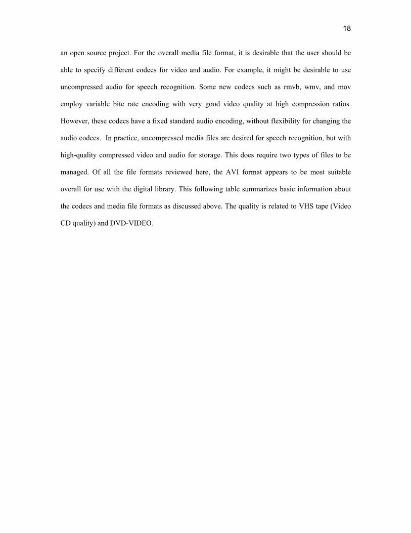
an open source project. For the overall media file format, it is desirable that the user should be
able to specify different codecs for video and audio. For example, it might be desirable to use
uncompressed audio for speech recognition. Some new codecs such as rmvb, wmv, and mov
employ variable bite rate encoding with very good video quality at high compression ratios.
However, these codecs have a fixed standard audio encoding, without flexibility for changing the
audio codecs. In practice, uncompressed media files are desired for speech recognition, but with
high-quality compressed video and audio for storage. This does require two types of files to be
managed. Of all the file formats reviewed here, the AVI format appears to be most suitable
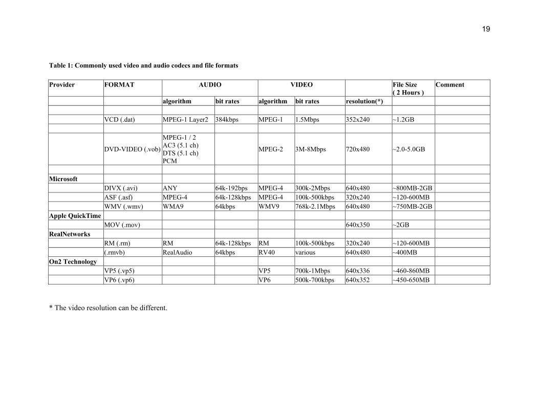
overall for use with the digital library. This following table summarizes basic information about
the codecs and media file formats as discussed above. The quality is related to VHS tape (Video
CD quality) and DVD-VIDEO.
19
Table 1: Commonly used video and audio codecs and file formats
Provider FORMAT AUDIO VIDEO File Size( 2 Hours )
Comment
algorithm bit rates algorithm bit rates resolution(*) VCD (.dat) MPEG-1 Layer2 384kbps MPEG-1 1.5Mbps 352x240 ~1.2GB
DVD-VIDEO (.vob)
MPEG-1 / 2 AC3 (5.1 ch) DTS (5.1 ch) PCM
MPEG-2 3M-8Mbps 720x480 ~2.0-5.0GB
Microsoft DIVX (.avi) ANY 64k-192bps MPEG-4 300k-2Mbps 640x480 ~800MB-2GB ASF (.asf) MPEG-4 64k-128kbps MPEG-4 100k-500kbps 320x240 ~120-600MB WMV (.wmv) WMA9 64kbps WMV9 768k-2.1Mbps 640x480 ~750MB-2GB Apple QuickTime MOV (.mov) 640x350 ~2GB RealNetworks RM (.rm) RM 64k-128kbps RM 100k-500kbps 320x240 ~120-600MB (.rmvb) RealAudio 64kbps RV40 various 640x480 ~400MB On2 Technology VP5 (.vp5) VP5 700k-1Mbps 640x336 ~460-860MB VP6 (.vp6) VP6 500k-700kbps 640x352 ~450-650MB
* The video resolution can be different.

20
Vocal Tract Length Normalization (VTLN)
Although high quality audio preserved with a "good" audio compression algorithm is
helpful for ASR accuracy, a completely speaker-independent ASR system is still subject to errors
due to variability arising from speaker differences. The ASR errors will create problems for
automated digital library creation of multimedia materials. In the remainder of this chapter, some
previous research for speaker normalization, the main research topic of this thesis, is summarized.
The most typical form of speaker normalization is a simple spectral transformation.
Assume SA(ω) and SB(ω) are long-term average spectra produced by speakers A and B. There are
many factors that cause differences in the long-term average spectra between two speakers
speaking the same speech materials. These factors include dialect, emphasis, miss-pronunciation,
and vocal tract-length differences. A normalizing spectral transformation is a mapping function
for one of the speakers, say speaker B, such that S'B(ω) = f(SB(ω)), and such that S'B(w) is similar
in some sense to SA(ω).
There has been much research that suggests that a major component of the speech
spectral variance between different speakers is because of different lengths of the vocal tract. The
human vocal tract is a basic physical component of the human anatomy that shapes the spectra of
sounds. For the speech recognition application, one of the traditional feature sets used are formant
frequencies, which are the peaks of the high-energy portions of the spectrum. These peaks are
determined by the resonances of the vocal tract, which are determined by overall length, and then
also by shape. For the case of vowels, in particular, the first two formant frequencies (F1, F2) of
each vowel signal are often used to project the speech signal to a two-dimensional pattern.
Beginning with the work of Peterson and Barney, it has been shown that vowels cluster
reasonably well in an F1-F2 space in the sense that the same vowels uttered by different speakers
have very similar values, and different vowels tend to have different F1-F2 values (Peterson and
Barney, 1952).

21
Although an F1-F2 space is a reasonably good feature space for recognizing vowels, the
vowel clusters in an F1-F2 space are large and overlap because of speaker differences. Thus, for
example, automatic vowel recognition rates based on F1 and F2 is much lower than rates obtained
by human listeners. One of the earliest reported attempts at vocal tract length normalization is that
of Wakita, who linearly scaled formant frequencies in a speaker specific way, in order to improve
the clustering properties of vowels in an F1-F2 space (Wakita, 1977). Wakita's approach is based
on theoretical work which shows that vocal tract length differences result in a linear scaling of
formant frequencies. In Wakita’s work, nine stationary American vowels were investigated.
Although there are many other investigations of speaker normalization, most other methods
require prior knowledge of the individual speaker. Wakita’s approach is physically based on a
general relationship between vocal tract length and formant locations, and the normalization is
accomplished without any prior knowledge of the speaker. The fundamental idea is that the vocal
tract configuration of each stationary vowel is the same for all speakers, but varies primarily in
vocal tract length. This is especially true when comparing male, female and child speakers.
Furthermore, Wakita showed that the changes in formant frequencies resulting from the
differences in vocal tract length can be compensated for by a simple equation.
iR
i FFl
l= (1)
Only the first three formant frequencies are adjusted by this equation, which implicitly
assumes a reference vocal tract length. As a result, the formant frequency projection area for each
vowel sound can be reduced to half or less of the original size.
There are many shortcomings of this approach, leaving room for improvements. The
normalization is based on comparisons of individual vowels, thus requiring that each speaker
utter the same vowels. It is not very convenient to make use of additional data from each speaker,
22
unless the new sounds are the same as those of the reference speaker. As also mentioned in the
paper, the formant frequency and length estimation is not very accurate. Additional methods for
normalizing for vocal tract length, based on various combinations of frequency shifts and warps
(Ono, Wakita, and Zhao, 1993; Tuerk and Robinson, 1993; Zahorian and Jagharghi, 1991).
In Ono et al’s paper, they investigate the relationship between spectral parameters and
speaker variations by a speaker-dependent shift of the spectra to improve the performance of a
speaker independent speech recognition system. The basic idea of their spectral shift techniques is
to shift individual filter band energies for each speaker to the band estimated to be that of the
reference speakers, based on the estimated vocal tract length.
Many researchers claimed that pitch is also one of the important parameters that can be
used to help normalize the acoustic properties of different speakers. Tuerk and Robinson
proposed a shift function based on each speaker’s geometric mean pitch frequency. The
normalization theory in their work is a modification of the auditory–perceptual work of Miller
(Miller, 1989). In Miller’s work, the transformed short-term spectral analysis of the input speech
signal can be equated to four pointers. The first three of the pointers (SF1, SF2, and SF3) relate to
formant frequencies and the fourth pointer SR is the speaker’s reference pitch, which is defined
as:
3000
ss
csss GMF
GMFGMFSR = (2)
The GMF0ss is the standard speaker’s geometric mean frequency, and the GMF0cs is the
current speaker’s mean frequency. Each formant frequency SF1, SF2, and SF3, then divided by
the SR and log scaled. The results are a set of coordinates in the auditory-perceptual space. Since
the formant ratio of F2-F1 and F3-F2 can be used to identify different vowels, the shift function
can adjust the location of formant frequencies, without changing identification. The processing

23
was tested by fist measuring the variance of the original data, then applying a speaker-specific
shift function dependent on the speakers mean pitch, and then re-examining the variance of the
shifted data. Relative to the original data, the variance was found to be reduced in the shifted set.
From a classifier point of view, the reduction of the variance helps test data to relocate to a
smaller area which improves the classification performance. In Tuerk and Robinson’s work, they
present a new linear function to further shift the coordinates to improve the performance.
Many of these VTLN methods are based on linear transformations. In Zahorian and
Jagharghi’s paper, the normalization is also derived from a physical basis. The frequency scale
for each speaker is re-scaled by a set of coefficients in a second order polynomial warping
function in the frequency domain. In particular, the frequency for each speaker is scaled by three
coefficients, a, b, and c, using.
cbfaff ++= '2''' (3)
In comparison to a linear transformation function, the second order polynomial function was
found to give a better mapping between unknown speakers and a reference speaker. The
coefficients were computed and stored by matching unknown and reference frequency patterns,
and finding coefficients such that the overall spectra of each unknown speaker and the reference
speakers would match as closely as possible. However, as in Wakita's earlier work, the method
required that the unknown and reference speaker utter the same sounds.
More recent work is focused on speaker adaptation to improve ASR for large-vocabulary
continuous speech recognition (Zhan and Westpa, 1997; Welling, Ney and Kanthank, 2002;
Gouvea, 1998). These references also summarize many of the general issues in speaker
adaptation by VTLN and provide a list of many related references on this topic. In Welling et al’s
work, the acoustic front end includes magnitude spectrum calculation, Mel frequency warping,

24
critical band integration, cepstral coefficient calculations, and additional parameter
transformations such as mean normalization and LDA. VTLN, for each speaker in training, and
each sentence in testing, is based on a piece-wise linear rescaling of the frequency axis applied to
the magnitude spectrum. The linear compression / expansion factor ranges from 0.88 to 1.12 with
a step size of 0.02 (13 total steps). The fundamental difficulty is that training of HMM model
parameters is in principle based on a separate optimization for each speaker, over both the
frequency scale parameter and all HMM parameters. Similarly, in recognition, optimal decoding
of the most likely word sequence for each sentence requires the consideration of each possible
frequency scaling for each sentence. The authors have presented several novel algorithmic
methods for improving performance and reducing computations, such as the use of single mixture
Gaussian densities in the first phase of training to determine VTLN scale factors, and
computationally efficient multi-pass approaches for both training and testing. The authors were
able to achieve error rate reductions on the order of 10-20% for several different ASR tasks
including digit strings and WSJ0.
Summary
In this chapter, several commonly used codecs and multimedia file formats were
discussed. Each of them has advantages and disadvantages because of original design goals.
Since we are mainly interesting in speech processing with better audio quality, the goal is to find
a multimedia file format with "reasonable" video quality at a high video compression, but with
the flexibility of a user specified and high quality audio codec to enable good performance for
automatic speech recognition. For the various multi-media formats surveyed, the avi appears to
be best for our work with the digital library.
We also surveyed some previous research for speaker normalization. Many researchers
attempted to determine a set of parameters, which could be normalized to remove differences
among speakers saying the same words. Thus, instead of retraining the classifier with each new

25
speaker, a much easier front-end normalization process could be used to improve recognition
performance. In this thesis, we purpose another normalization procedure by comparing the long-
term spectral template of a pre-selected typical speaker with each new speaker to improve
recognition performance. In chapter three the normalization process is described in detail;
experimental results are given in chapter four.
26
CHAPTER III
NORMALIZATION ALGORITHM DESPCRIPTION
Introduction
The normalization method is based on determining speaker specific frequency ranges and
scale factors, such that a spectral template for each speaker best matches, in a mean square error
sense, a spectral template for a selected typical speaker, with the goal of improving automatic
speech recognition. Generally speaking, speaker dependent automatic speech recognition systems
are more accurate than speaker independent systems. However, for many applications including
the case of digital libraries, it is difficult or impractical to obtain specific speech data from the
speaker to re-train the classifier to improve the accuracy. In the work reported here, the basic idea
is to create a spectral template of the high energy portions of a speech database for a typical
speaker and then, for each training and testing speaker, to adjust frequency ranges and scale
factors so that spectral templates computed for each speaker best match the typical speaker
template. The parameters used to make the match are the low frequency band edge, the high
frequency band edge, and a warping factor. The algorithm searches through all the possible
combination of these three parameters to obtain the closest mean square error (MSE) match of
each speaker’s spectral template to the typical speaker template. Using this new frequency range
and scale factor for each speaker, the classifier is trained using normalized speech features.
The Algorithm Description
The algorithm consists of the following two primary steps for Vocal Tract Length
Normalization. First, create a spectral template for a selected “typical” speaker, using a frequency
range and scaling factor expected to be nominal. Represent this spectral template with DCTC

27
parameters. Second, for each additional training and testing speaker, compute a spectral template.
Then, determine values of low frequency (FL), high frequency (FH), and warping factor (α), such
that a spectral template computed with this new frequency scale better matches the template of
the typical speaker. Two methods were investigated to obtain FL, FH, and α. In one, FL and FH
are first determined based on the frequency range each speaker appears to use, and then α is
determined by search methods. In the other method, all three parameters are determined by a
three-dimensional search process. The set of FL, FH, and α is obtained such that the weighted
mean square error difference between the DCTCs of the speaker and the DCTCs of the typical
speaker is minimized. The resultant values for FL, FH, and α are then considered as a parametric
representation of the spectral template for each speaker. Normalized parameters (DCTC values
computed using a normalized frequency range and scaling) can then be used as front-end features
for an ASR system. Many variations of this basic approach, and many experimental evaluations,
are reported in this work.
In addition to the algorithm mentioned above, another approach was investigated
whereby the frequency scaling parameters were adjusted so as to optimize automatic vowel
classification performance for “testing” data for each test speaker. The classifier was trained only
once. The training speakers are still first parameterized using normalized features from the
minimum mean square error approach. However, the frequency ranges and scaling factor
parameters of each testing speaker are re-adjusted so that classification accuracy is maximized.
Although this approach is not really fair, since "testing" data is used to some extent in training,
this method can be viewed as a control indicating the upper limit of possible recognition
performance. Each of these steps is explained and illustrated in more detail below.
Spectral Processing
In this work, for each training and testing speaker, all selected sentences (ten sentences or
about 30 seconds of speech in this work) were combined into a single array containing the

28
samples of the acoustic speech signal. The speech signal was then pre-emphasized using the
second order equation.
)2(64.0)1(49.0)1(95.0)()( −−−∗+−∗−= nynynxnxny (4)
This type of pre-emphasis simulates the frequency response of human hearing, and is
commonly used as a first step in speech processing for automatic speech recognition systems. For
the filtered sequence of data, the short-time spectrum was computed, using a frame length of
30ms and a frame spacing of 15ms. This short-time spectrum (called a spectrogram) gives the
distribution of the speech energy over time and frequency. From a spectrogram, the unvoiced and
voiced portions of speech are quite apparent. In particular, in a previous study (Kasi and
Zahorian, 2002), it was demonstrated that the normalized low frequency energy ratio (NFLER) is
a good indicator for voiced versus unvoiced speech. NFLER is determined by computing the
energy in each frame over the frequency range of 100 Hz to 900 Hz, and then normalizing (i.e.,
dividing) by the average energy in that range, over the entire utterance. Experiments showed that
those frames with NLFER above 0.75 are nearly always voiced and those frames with NFLER
below .5 are nearly always unvoiced. Thus, except for the uncertainty in the regions of the speech
signal when NFLER is between .5 and .75, NFLER is a reliable indicator of voiced versus
unvoiced speech. Thus, for the purposes of creating a spectral template using only the voiced
portions of the speech, frames were selected with NLFER greater than 0.75. This procedure
insured that only voiced frames were used to create the spectral template.
There are two main reasons that we decided to create speech templates based only on the
voiced speech. First, since the experiments were conducted only for vowels, which are voiced, it
seemed logical to assume that the spectral templates should be based only on the same type of
speech. However, in addition, pilot tests were done to compare results using spectral templates
29
created only from voiced speech versus spectral templates created from all the speech. In these
tests, it was found that normalization based on the voiced spectral templates was slightly better
(i.e., higher recognition results).
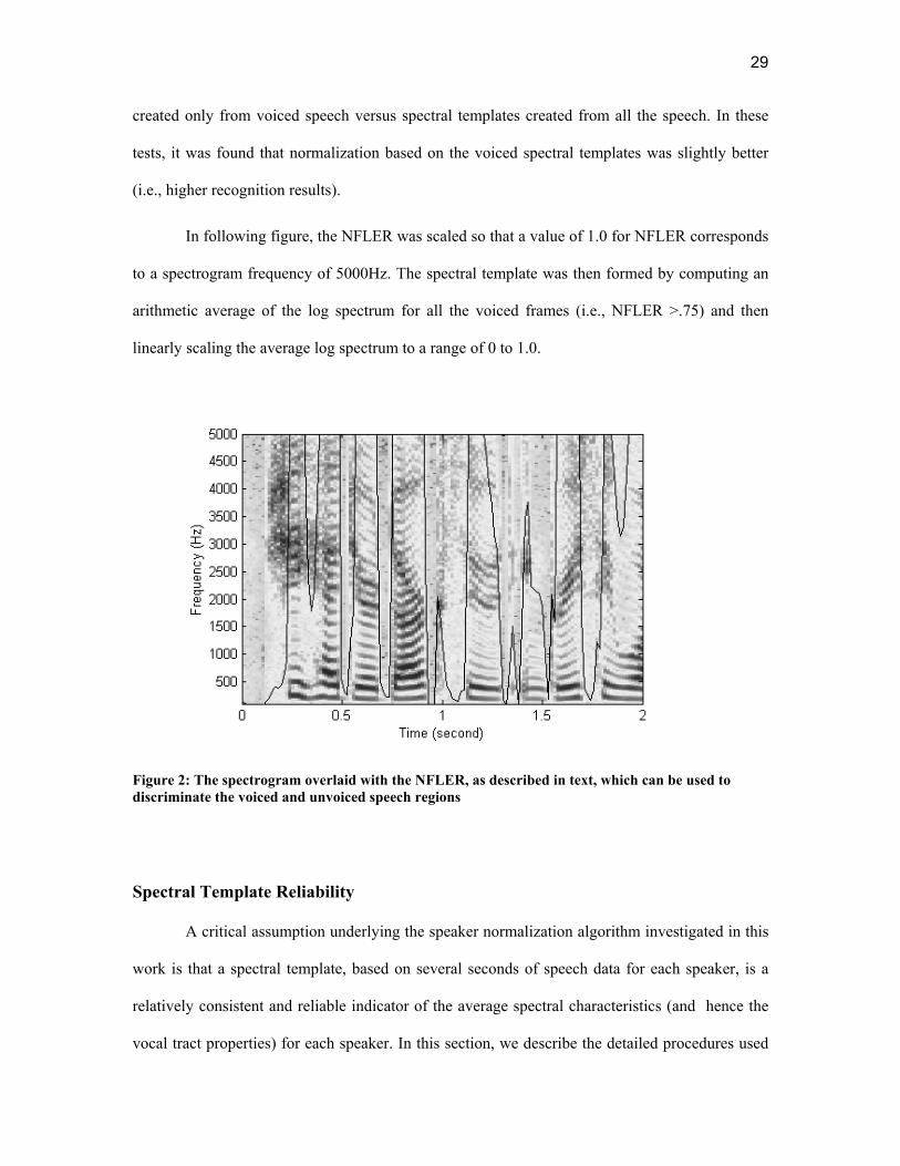
In following figure, the NFLER was scaled so that a value of 1.0 for NFLER corresponds
to a spectrogram frequency of 5000Hz. The spectral template was then formed by computing an
arithmetic average of the log spectrum for all the voiced frames (i.e., NFLER >.75) and then
linearly scaling the average log spectrum to a range of 0 to 1.0.
Figure 2: The spectrogram overlaid with the NFLER, as described in text, which can be used to discriminate the voiced and unvoiced speech regions
Spectral Template Reliability
A critical assumption underlying the speaker normalization algorithm investigated in this
work is that a spectral template, based on several seconds of speech data for each speaker, is a
relatively consistent and reliable indicator of the average spectral characteristics (and hence the
vocal tract properties) for each speaker. In this section, we describe the detailed procedures used

30
to create spectral templates, and give results that indicate that the spectral template is indeed a
reliable stable indicator of the average spectral characteristics of each speaker.
In the TIMIT speech database, which was used for the experiments reported in this thesis,
there are ten sentences for each speaker. Since each sentence is only 2 to 3 seconds long, it was
necessary to make sure that the spectral template computed from a small number of sentences are
a good representation of the long term spectral characteristics of each speaker. Although longer
speech data gives a better representation, there are also disadvantages such as the need for
acquiring the longer speech sample and more computations. In actual applications, long speech
materials may simply not be available. Therefore, experiments were conducted with one sentence,
two sentences, and five sentences to examine the degree to which spectral templates vary as a
function of speech length. The following figures depict long-term average spectral template using
one, two, and five sentences from the same speaker.
0 1000 2000 3000 4000 5000 6000 7000 8000
6
8
10
12
14
16
18
20
22
Hz
log
ampl
itude
Spectral Template (3 second long speech data)
data1data2data3data4
Figure 3: Comparison of 4 different spectral templates of a speaker, each computed from approximately 3 seconds (1 sentence) of speech
The graphs in Figure 3 depict four spectral templates from the same speaker. Each
colored line indicates the spectral template from a single (different) sentence. The content of each
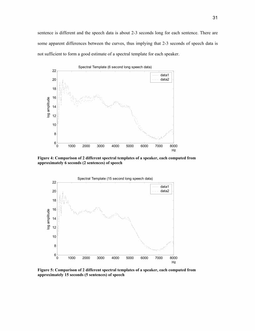
31
sentence is different and the speech data is about 2-3 seconds long for each sentence. There are
some apparent differences between the curves, thus implying that 2-3 seconds of speech data is
not sufficient to form a good estimate of a spectral template for each speaker.
0 1000 2000 3000 4000 5000 6000 7000 80006
8
10
12
14
16
18
20
22
Hz
log
ampl
itude
Spectral Template (6 second long speech data)
data1data2
Figure 4: Comparison of 2 different spectral templates of a speaker, each computed from approximately 6 seconds (2 sentences) of speech
0 1000 2000 3000 4000 5000 6000 7000 80006
8
10
12
14
16
18
20
22
Hz
log
ampl
itude
Spectral Template (15 second long speech data)
data1data2
Figure 5: Comparison of 2 different spectral templates of a speaker, each computed from approximately 15 seconds (5 sentences) of speech

32
This graph in Figure 5 depicts two long term spectral templates from the same speaker.
Each spectral template was created from approximately 15 seconds of speech data (5 sentences).
Even though each of the five sentences corresponds to totally different speech materials, the two
spectral templates match very closely. Note that the graphs shown in Figure 4, each obtained
from two sentences of speech data, are more similar to each other than the graphs depicted in
Figure 3, but not as similar as the two graphs shown in Figure 5. Thus, as expected, the spectral
templates are more reliable indicators of the long term spectrum, as a longer speech length is
used.
In the speaker normalization experiments reported in chapter 4, all ten sentences were
used for template creation. Thus, the total speech duration for each speaker was typically between
20 and 30 seconds. Spectral template based on ten sentences are the most accurate possible with
the TIMIT speech database, since the database contains only ten sentences for each speaker.
Discrete Cosine Transform
The spectral templates were parametrically encoded with a Discrete Cosine Transform
(DCT). In the following few paragraphs, we describe the procedure used to compute the DCT. For
ease of explanation, consider X(f) to be the continuous magnitude spectrum represented by the FFT,
encoded with linear amplitude and frequency scales. Before the Discrete Cosine Transform
Coefficients (DCTCs) are computed, X(f) is first rescaled using perceptual amplitude and frequency
scales, and relabeled as X'(f). The relationship between the X(f) and the X’(f’) is defined by the
following equations.
, , )(' fgf = ))(()(' ' fXafX = dfdfdgdf =' (5)

33
A selected range of f, that is from FL to FH, is first linearly scaled and shifted to a range of 0 to 1.
Similarly g is constrained so that f’ is also over a 0 to 1 range. In all of this work, g was the
bilinear transformation given by the formula.
−+== −
)2cos(1)2sin(tan1)( 1'
fffffgπα
παπ
(6)
Thus g is parametrically encoded with a single parameter, α, which is referred to as the warping
scale factor. Figure 6 illustrates the warping function, with values of α equal to 0.45, 0, and -0.45.
Typically an α value of 0.45 is used for automatic speech recognition applications.
0 0.1 0.2 0.3 0.4 0.50
0.1
0.2
0.3
0.4
0.5
f
f'
Figure 6: Bilinear transformation with α = 0.45 (dash-dot line), 0 (dotted line), and -0.45 (dashed line)
The nonlinear amplitude scaling, “a”, in practice is typically a logarithm, since amplitude
sensitivity in hearing is approximately logarithmic. The next step in processing is to compute a
cosine transform of the scaled magnitude spectrum. The DCTC values, computed as in equation 6
below, can be considered as acoustic features for encoding the perceptual spectrum:

34
(7) ')'cos()'(')(1
0
dffifXiDCTC ∫ ∗∗∗= π
By substitution in equation 7, and replacing "a" by log
∫ ∗∗∗=1
0
))(cos())(log()( dfdfdgfgifXiDCTC π (8)
Also, we can redefine the basis vectors as
dfdgfgifi ))(cos()( ∗∗= πφ (9)
so the final equation for computing the DCTCs becomes
(10) dfffXiDCTC i )())(log()(1
0
φ∗= ∫
For the actual processing, all discrete spectral values are computed with FFTs and the
equation above changes to a summation:
(11) )())(log()(2
1
nnXiDCTCN
Nni∑
=
∗= φ

35
where n is a an FFT index, and N1 and N2 correspond to the lowest and highest frequencies used in
the calculation. The calculation of these modified cosine basis vectors is very similar to the
calculation of cepstral coefficients. However, in line with our previous work, we call these terms
Discrete Cosine Transform Coefficients (DCTC), (Zahorian and Nossair, 1999), rather than
cepstral coefficients. Note that the DCTCs are also coefficients that represent a smoothed version of
the scaled spectrum and it is thus very easy to compute the smoothed spectrum from the DCTCs.
From the Vocal Tract Length Normalization point view, this method for DCTC
calculations is very convenient, since speaker-normalized DCTC coefficients can be computed
directly from the FFT spectrum, using only three normalization parameters, low frequency (FL),
high frequency (FH), and warping factor (α), to control the normalization.
The combination of using DCTC representations and VTLN is illustrated in Figure 7. The
top panel of the Figure 7 (a) shows the original spectral template of a single female speaker over a
frequency range of 0 Hz to 8000 Hz, as well as the DCTC smoothed version of this spectrum (FL
= 100 Hz, FH = 5000 Hz, and α = 0.45). The bottom panel (b) shows a similar graph of the DCTC
smoothed spectrum of a male speaker.

36
0 1000 2000 3000 4000 5000 6000 7000 80000
0.2
0.4
0.6
0.8
1
Hz
norm
aliz
ed lo
g am
plitu
de
(a) female speaker
0 1000 2000 3000 4000 5000 6000 7000 80000
0.2
0.4
0.6
0.8
1
Hz
norm
aliz
ed lo
g am
plitu
de
(b) male speaker
original spectranormalized spectra
original spectranormalized spectra
Figure 7: Illustration of original spectral template (dashed curve) and DCTC smoothing of spectrum by using FL, FH, and α (dotted curve) of a female speaker (a) and a male speaker (b). See text for more complete description

37
Determination of FL, FH, and α
For this work, two methods were used for the actual template matching. In the first
method, FL and FH, were first determined independently by separate algorithms for all speakers,
including the typical speaker. In particular, FL was determined by computing the average F0 in the
speech utterance, and then letting FL equal to ½ that average F0 value. FH was determined by
searching the amplitude-normalized spectral template, from FS/2 toward lower frequencies, and
setting FH equal to the frequency at which the spectral template is first higher than some threshold
(typically 0.1 times the maximum value). Thus the objective here was to first determine the
frequency range used by each speaker, based only on the spectral template of that speaker.
For this first method, α was set to .45 for the typical speaker. Then, for all other speakers,
α was adjusted to minimize the mean square error (as described below) between the DCTCs of
that speaker and the typical speaker, but using the frequency ranges found as described in the
preceding paragraph.
In the second method of the spectral template matching, the low frequency limit (FL), the
high frequency limit (FH), and warping factor α were set to nominal values (100 Hz, 5000 Hz, and
0.45) for the typical speaker. Using these three values for the parameters, FL, FH, and α, a set of
"warped" cosine basis vectors over frequency (referred to as bvF matrix) were computed. This
matrix was then used to convert the spectral template of the speech signal for the typical speaker
to 15 DCTC coefficients. These 15 DCTCs thus form a 15-dimensional representation of the
spectral template for the typical speaker. After the typical speaker template was created, for all
remaining speakers in the database, speaker specific values of FL, FH and the α were computed
such that DCTCs computed for each of the speakers with speaker specific frequency parameters
best match the DCTCs of the typical speaker template. That is, for each speaker, determine FL,
FH, and α, such that
38
15,))())(( 2
1=−=∑
=
NkDCTCkDCTCerror T
N
kU (12)
is minimized. In the equation, U denotes the both training and test (unknown) speaker and T
denotes the typical speaker.
Figure 8 illustrates the spectral template matching procedure, both in the frequency
domain (upper panel), and in the DCTC parameter space (lower panel). In the top panel, the
dashed and dotted lines are spectral templates from the "typical” speaker (dashed) and an
arbitrary "test" speaker (dotted), before any frequency adjustments were made. The dash-dot
curve is the template for the test speaker, but after the Minimum Mean Square Error was
minimized. The lower panel in the figure depicts the DCTC differences between the typical
speaker and the unknown new speaker both before and after the Mean Square Error was
minimized.
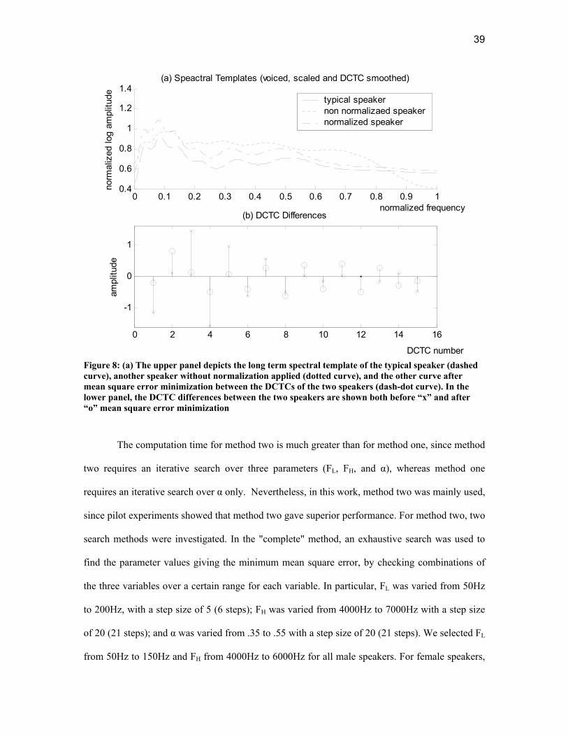
39
0 0.1 0.2 0.3 0.4 0.5 0.6 0.7 0.8 0.9 10.4
0.6
0.8
1
1.2
1.4
normalized frequency
norm
aliz
ed lo
g am
plitu
de
(a) Speactral Templates (voiced, scaled and DCTC smoothed)
0 2 4 6 8 10 12 14 16
-1
0
1
DCTC number
ampl
itude
(b) DCTC Differences
typical speakernon normalizaed speakernormalized speaker
Figure 8: (a) The upper panel depicts the long term spectral template of the typical speaker (dashed curve), another speaker without normalization applied (dotted curve), and the other curve after mean square error minimization between the DCTCs of the two speakers (dash-dot curve). In the lower panel, the DCTC differences between the two speakers are shown both before “x” and after “o” mean square error minimization
The computation time for method two is much greater than for method one, since method
two requires an iterative search over three parameters (FL, FH, and α), whereas method one
requires an iterative search over α only. Nevertheless, in this work, method two was mainly used,
since pilot experiments showed that method two gave superior performance. For method two, two
search methods were investigated. In the "complete" method, an exhaustive search was used to
find the parameter values giving the minimum mean square error, by checking combinations of
the three variables over a certain range for each variable. In particular, FL was varied from 50Hz
to 200Hz, with a step size of 5 (6 steps); FH was varied from 4000Hz to 7000Hz with a step size
of 20 (21 steps); and α was varied from .35 to .55 with a step size of 20 (21 steps). We selected FL
from 50Hz to 150Hz and FH from 4000Hz to 6000Hz for all male speakers. For female speakers,

40
FL was varied from 100Hz to 200Hz and FH was varied from 5000Hz to 7000Hz. The same range
of α was used for both male and female speakers. An exhaustive search of all these combinations
thus required a total of 6 x 21 x 21 or 2664 steps, in the search process for each speaker. After
experimental verification that the error surface was relatively smooth, a much faster search
technique was adopted with termination of the search in all directions for which the error was
found to be increasing. This method was found to reduce the number of calculations by
approximately a factor of 10 with very little change in performance relative to the more complete
search of the parameter space.
A file for each speaker was generated consisting of the frequency ranges and scaling
factor (FL, FH, and α), and remaining DCTC differences for each training and test speaker. This
parameters were then used for additional processing and for vowel classification experiments.
Front-End Feature Adjustment using Normalization Parameters
In the original DCTC features extraction function (no speaker normalization), the
spectrum was computed for 30ms frames with 15 ms frame spacing over the entire speech data
available for that speaker. Then the DCTC features were computed by multiplying with the
cosine basis matrix. To be able to use the new frequency ranges and scaling factor, an additional
flag was added to the feature calculation function. In particular, the normalization can be either
enabled. When the normalization is disabled, the FL, FH and α are based on the standard settings;
typical, FL is equal to 100Hz, FH is equal to 5000Hz, and α is equal to 0.45 for each frame. When
the normalization is enabled, the parameters are replaced by the speaker-specific values of FL, FH
and α, and the DCTC differences are (optionally) added to the DCTC features.
Parameter Adjustment Based on Classification performance
As mentioned earlier, in order to examine the upper limit of performance possible based
on adjustments of the three parameters of frequency, additional experiments were conducted with

41
parameters adjusted so as to maximize classification performance for each speaker. In particular,
the spectral template matching described above (based on minimum mean square error matching)
was first implemented for each training and test speaker. A neural network vowel classifier was
then trained using the normalized data of each training speaker. This trained neural network was
then used to iteratively evaluate each test speaker, with further adjustments then made in FL, FH,
and α for each test speaker so as to maximize classification performance. Of course, these tests
are not really good indicators of test performance, since the test data does effectively become part
of the training data. However, the results obtained with this method do give an indication of the
performance improvements possible by adjusting only three parameters that control the frequency
range and scale for each speaker.
Normalization based on DCTC differences
Finally, since the fundamental assumption of this normalization is that the mean square
difference between the DCTCs of the typical speaker template and that of each underlying
speaker should be minimized, the average DCTC values for each speaker, including the typical
speaker, were computed after normalization by the frequency parameters. These speaker-specific
average DCTC values could then be subtracted from the DCTCs of each speaker after the
frequency domain adjustments described above. After this subtraction, the DCTCs of each
speaker would have a mean value of 0.0, thus also presumably reducing the variability in DCTCs
among speakers.
Summary
In this chapter, we described the normalization procedure in detail. By comparing long term
spectral template from the typical speaker and each training and test speaker, the average spectral
differences between speakers can be reduced, potentially improving classifier accuracy. Methods
presented were:

42
1. Algorithmic methods to determine the frequency range, defined by parameters FL and FH,
followed by error minimization to compute the nonlinear scaling parameter α.
2. An error minimization method to find the simultaneous best fit of all three normalization
parameters FL, FH, and α.
3. Method 2, above followed by additional adjustments of the parameters FL, FH, and α so as
to maximize classification accuracy.
4. Either method 1 or 2, followed by subtraction of the DCTC averages for each spectral
template.
With minor modifications of the front-end speech analysis feature extraction procedure, we
can avoid the computational burden of re-training the classifier for each new speaker and
hopefully further improve classifier accuracy. In the next chapter, the experimental work is
presented which evaluates the speaker normalization method.

43
CHAPTER IV
EXPERIMENTAL EVALUATION
TIMIT Database
All experiments reported in this thesis were conducted with the TIMIT database of
sentences. The DARPA TIMIT database is acoustic-phonetic speech data, which was designed to
provide phonetically labeled acoustic data for the development and evaluation of automatic
speech recognition systems. It was developed as a joint effort between Texas Instruments (TI)
and MIT, funded by DARPA, in 1986. (DARPA Speech Recognition Workshop, 1986) It consists
of utterances of 630 speakers that represent the major dialects of American English, as subdivided
by regions at U.S. There are totally eight different regions represented as shown below:
Folder Area ------------- ---------------------------------------------------- dr1 New England dr2 Northern dr3 North Midland dr4 South Midland dr5 Southern dr6 New York City dr7 Western dr8 Army Brat (moved around)
The TIMIT speech database is organized in 2 categories, a training data set that
includes 420 speakers, and a test data set that includes 210 speakers. There are ten sentences for
each speaker. For each speaker, there are three different sentence types; (1) ”sa” consists of 2
(same sentence for all speakers) sentences per speaker which are considered as SRI dialect
calibration sentences; (2) “si” consists of 3 (different) sentences per speaker which are referred to
as TI (Texas Instruments) random contextual variants sentences; and (3) “sx” consists of 5

44
(different) sentences per speaker, which are the MIT phonetically compact sentences. In our
work, we used small training data sets and large test data sets. Therefore the training and test data
sets, as mentioned above, were not used. The actual training and test database subsets of TIMT
are described below.
Brief Description of Experimental Database
The normalization methods described in chapter three were evaluated using a neural
network classification of 10 monophone vowels (/aa/, /iy/, /uw/, /ae/, /er/, /ih/, /eh/, /ao/, /ah/, and
/uh/) taken from the TIMIT database. In the TIMIT database, there are many more male speakers
than female speakers. In the experiments reported here, we did not use the defined training and
test data sets. Instead, we selected speakers more suitable for our experimentation. In Experiment
1 and Experiment 3, there are totally 4 different configurations of interest: (1) no normalization,
(2) normalization based on FH, FL, and α, (3) normalization based on FH, FL, α, and DCTC
averages, and (4) normalization based on FH and FL only. Also, three data configurations were
used, consisting of three different training sets, and three different testing sets; (1) 50 female
training speakers with 120 male or female testing speakers; (2), 50 male training speakers with
120 male or female testing speakers; (3) 25 male plus 25 female (a total of 50) training speakers
with 60 male plus 60 female (a total of 120) testing speakers. The total number of vowel training
tokens was either 3584 (female training), 3424 (male training), or 3462 (mixed training set). The
total number of vowel tokens for testing was either 8336 (female testing), 8139 (male testing),
and 8126 (mixed testing set).
Experiments 1, 2, and 3 were conducted with a back-propagation neural network
classifier with one hidden layer of 10 hidden nodes. Each neural network had 15 input nodes,
which equals the number of features generated by the front-end analysis. Each network had 10
output nodes, one for each to indicate each vowel. Although 10 hidden nodes were used for most
of the results presented in this chapter, in experiment 4, the changes in classification accuracy due

45
to varying the number of hidden nodes are also reported. Finally, one series of tests was done
with a maximum likelihood classifier.
Long-Term Spectral Template Matching Experiment
In chapter three, we mentioned two different approaches for finding the three
normalization parameters. The first method is to first determine FL and FH based on intrinsic
properties of each spectral template, and to compute α to minimize the mean square error between
two spectral templates. The second method is based on a simultaneous error minimization
solution of three normalization parameters, so this gives many possible combinations of the three
parameters to consider. Although the second method is highly time consuming, pilot experiments
indicated that higher recognition rates were obtained with the second method than for the first
method. Thus, all the experiments reported in this chapter were conducted using the second
method.As mentioned in Chapter 3, if the speech signal has a longer duration, the spectral
template computed from the longer duration signal should be a more "reliable" estimate of
spectral characteristics of the speaker, and the three normalization parameters, FH, FL, and α,
computed from such a template should be consistent estimates for each speaker. That is, if these
three parameters were computed from a spectral template computed from a different speech
segment from the same speaker, the three parameters should have the same or nearly the same
values. To experimentally test this assumption, spectral templates were computed for speech
segments consisting of two, five, and ten sentences, which varied the speech duration from
approximately 6 seconds to 30 seconds. The three normalization parameters, FL, FH, and α, were
then computed for each spectral template, using the same typical speaker reference. The
following three figures illustrate the variations in the three normalization parameters as a function
of speech duration (two, five, and ten sentences) for each of 20 speakers. The method used here is
the full search of the three normalization parameters, FL, FH, and α.

46
Frequency Low
020406080
100120140160
1 3 5 7 9 11 13 15 17 19
speaker number
Hz2 sentences5 sentences10 sentences
Figure 9: FL values as obtained from spectral templates computed from 3 different speech lengths for each of 20 speakers
Figure 9 depicts the minimum mean square error obtained value of FL for each test
speaker, using templates obtained from two, five, or ten sentences. The x-axis is represents test
speaker indices, using randomly selected female speakers (speakers 1-13) and randomly selected
male speakers (speakers 14-20). The y-axis is the computed FL value (search range of 50-150Hz
for male speakers and 100-200Hz for female speakers) for each of the three template lengths.
Frequency High
4900
5000
5100
5200
5300
5400
5500
1 3 5 7 9 11 13 15 17 19
speaker number
Hz2 sentences5 sentences10 sentences
Figure 10: FH values as obtained from spectral templates computed from 3 different speech lengths for each of 20 speakers
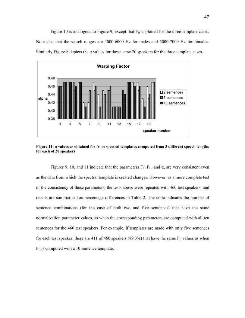
47
Figure 10 is analogous to Figure 9, except that FH is plotted for the three template cases.
Note also that the search ranges are 4000-6000 Hz for males and 5000-7000 Hz for females.
Similarly Figure 8 depicts the α values for these same 20 speakers for the three template cases.
Warping Factor
0.38
0.40
0.42
0.44
0.46
0.48
1 3 5 7 9 11 13 15 17 19
speaker number
alpha2 sentences5 sentences10 sentences
Figure 11: α values as obtained for from spectral templates computed from 3 different speech lengths for each of 20 speakers
Figures 9, 10, and 11 indicate that the parameters FL, FH, and α, are very consistent even
as the data from which the spectral template is created changes. However, as a more complete test
of the consistency of these parameters, the tests above were repeated with 460 test speakers, and
results are summarized as percentage differences in Table 2. The table indicates the number of
sentence combinations (for the case of both two and five sentences) that have the same
normalization parameter values, as when the corresponding parameters are computed with all ten
sentences for the 460 test speakers. For example, if templates are made with only five sentences
for each test speaker, there are 411 of 460 speakers (89.3%) that have the same FL values as when
FL is computed with a 10 sentence template.

48
Table 2: The percentage of speakers such that FL, FH, and α exactly match (columns 1and 2) and percentage of speakers for which matches are within +1 or -1 search steps (column 3 and 4), when 2 or 5 sentences are used
exact matched +1 or -1 step matched 5 sentences 2 sentences 5 sentences 2 sentences number of same FL 89.6% 82.6% 97.4% 95.2% number of same FH 84.6% 81.1% 97.6% 92.8% number of same α 47.2% 39.8% 95.2% 83.7%
Although the percentage of exact matches for α is only 40–50%, the normalization
parameters generally do not vary much when the templates change. For example, as Table 2
shows, the percentage of speakers for which the normalization parameters match to within +1 or -
1 step of the search range is typically over 90%. Nevertheless, since spectral templates based on
longer speech intervals should give the best representation of the average spectrum of each
speaker, all ten sentences were used for each test speaker in the following experiments. In actual
applications, it appears that the long term spectral template should be based on 30 seconds or
more of speech, so that the normalization parameters FL, FH, and α will accurately represent the
spectral characteristics of each speaker.
In summary, the experimental results presented in this section, along with the spectral
template plots given in chapter 3, are reasonable evidence that the spectral templates based on all
10 sentences available in the TIMIT database for each speaker are quite good representations of
the average spectrum for each speaker. It was also simply not possible to test with even longer
speech durations.
Experiment Set 1: General Effect of Normalization for Various Combinations of the
Normalization Parameters and Various Combinations of Training and Test Data
The primary goal of these experiments was to determine the general effects on vowel
classification performance of the normalization for various combinations of normalization
parameters, including the entire set. As specific sub goal was to determine if, for the case when

49
training and test speakers are deliberately mismatched as to speaker gender, the frequency axis
normalization could eliminate the systematic differences between parameters computed from
female speakers and male speakers. Test results, in terms of test classification results for the
vowels, are presented in Table 3, 4 and 5.
Table 3: Vowel classification rates for training and test data, with gender matched training and test data, for various parameters used to control the normalization
speaker gender condition (Male vs Male) (Female vs Female) Training data Test data Training data Test data number of speakers 50 120 50 120 number of sentences 500 1200 500 1200 no spkn 71.6% 66.5% 69.5% 64.7% spkn, (FL, FH, α, DCTC) 68.3% 65.5% 68.8% 64.1% FL, FH, and α 67.9% 65.6% 68.6% 63.5% FL, FH 71.0% 67.0% 69.8% 65.8%
Referring to Table 3, the first two rows of data are the numbers of sentences and speakers
for each training and test data set. For the case of Table 3, the training and test data sets are
matched in terms of speaker gender. The remaining rows of data are vowel classification results
for various normalization conditions. The third row lists the classification accuracy without any
normalization. The normalization parameters are selectively applied to the test speakers in each of
the following rows. For two of the cases (rows 4 and 5), the normalization procedure appears to
result in a 1 to 2% drop in classification accuracy. The only case for which the normalization
results in a slight improvement is when only FL and FH are applied, which gives approximately a
0.5 to 1% improvement.

50
Table 4: Vowel classification rates for training and test data, with gender mismatched between training and test data, for various parameters used to control the normalization
speaker gender condition (Male vs Female) (Female vs Male) Training data Test data Training data Test data number of speakers 50 120 50 120 number of sentences 500 1200 500 1200 no spkn 71.6% 44.4% 69.5% 48.2% spkn, (FL, FH, α, DCTC) 68.3% 60.9% 68.8% 62.7% FL, FH, and α 67.9% 60.3% 68.6% 63.4% FL, FH 71.0% 61.9% 69.8% 64.0%
Table 4 is arranged the same as is Table 3. The primary difference from Table 3 is that
training and test speakers are from different genders in Table 4. With no speaker normalization,
test results are much lower than comparison results for the gender matched training and testing
results with no normalization. Additionally, for this gender mismatched case, test results are
improved about 17% relative to non-normalized results (61% versus 44%). Furthermore, the
"best" normalization is that based only on FL and FH. However, even the normalized test data
results shown in Table 4 are lower than all the test results given in Table 3.
Table 5: Vowel classification rates for training and test data, with gender mixed training data and female or male test data, for various parameters used to control the normalization
speaker gender condition (Male&Female vs Female) (Male&Female vs Male) Training data Test data Training data Test data number of speakers 25-25 120 25-25 120 number of sentences 250-250 1200 250-250 1200 no spkn 68.1% 61.7% 68.1% 64.3% spkn, (FL, FH, α, DCTC) 68.5% 63.4% 68.5% 65.4% FL, FH, and α 68.3% 63.1% 68.3% 65.3% FL, FH 69.7% 64.1% 69.7% 65.0%
Finally, in Table 5, results are given when the training data is a mixture of male and
female speakers, but test speakers are either only male or only female. For the case of female test
speakers, the normalization results in about a 4% improvement relative to the non-normalized

51
results. However, for the case of male test speakers, the normalization results in less than 1%
improvement.
Experiment Set 2: Classification Results with Mixed Training and Test Speakers for
Various Typical Speakers
This experiment was designed as a further investigation of the normalization procedure
presented in this thesis, but using a mixture of male and female speakers for both training and
testing. For these tests, only FL and FH, shown to be most effective in Experiment 1, were used for
normalization. Results are given in Table 6. The normalization results in about a 2%
improvement of test results, as compared to no normalization.
Table 6: Vowel classification rates for training and test data, both with mixed gender training and test data, for various parameters used to control the normalization
speaker gender condition (Male&Female vs Male&Female) Training data Test data number of speakers 25-25 60-60 number of sentences 250-250 600-600 no spkn 68.1% 63.5% spkn, (FL, FH, α, DCTC) 68.5% 64.4% FL, FH, and α 68.3% 64.2% FL, FH 69.7% 65.2%
Additionally, we tested the performance of the system, using each of the training speakers in the
training database as the typical speaker. Typical test results are shown in Table 7. Test results for
the different typical speakers are shown for the four "best” and four "worst” typical speakers.

52
Table 7: Test results for mixed speakers types (male and female), without normalization (row 1), and with normalization, but using different training speakers as the “typical” speaker in the training process
speaker gender condition (Male vs Female) no normalization 63.5% 1. (FL, FH), female 65.2% 2. (FL, FH), male 64.7% 3. (FL, FH), female 63.8% 4. (FL, FH), female 63.2% 1. (FL, FH), male 61.3% 2. (FL, FH), male 62.5% 3. (FL, FH), female 62.8% 4. (FL, FH), male 62.9%
Experiment Set 3: Parameter Adjustment by Classification Performance
As mentioned earlier, the DCTC coefficients can be computed from the log spectrum
using only FL, FH, and α to adjust the normalization. In this experiment, a further investigation
was conducted using neural network classification performance accuracy to guide the adjustment
of parameters. First, the method mentioned for experiment 1 was performed to evaluate the
baseline performance accuracy. Secondly, using the neural network trained from the normalized
training data, the FL, FH, and α for each test speaker was used and the performance accuracy for
each test speaker was calculated individually. Next, using the fixed neural network based on the
training speakers, the three parameters, FL, FH, and α were adjusted for each test speaker (but
considering one speaker only at a time), until the maximum performance accuracy was reached
for each test speaker. These tests were very time consuming, since a very large number of tests
were needed for each speaker, since classification performance did not seem to depend
“smoothly” on parameter adjustments.

53
0.0%10.0%20.0%30.0%40.0%50.0%60.0%70.0%80.0%90.0%
100.0%
1 2 3 4 5 6 7 8 9 10 11 12 13 14 15 16 17 18 19 20
speaker number
%M.S.E. normalizedN.N normalized
Figure 12: Test results using procedure similar to that used for experiment 1, but considering each test speaker individually for 20 test speakers
Test results were obtained using the same procedure used for experiment 1, but results
are shown for test speaker individually. Results for 20 speakers are given in Figure 12. The bars
labeled “Mean Square Error” are test classification results obtained when parameter adjustments
for each test speaker are based on minimum mean square error methods. The bars labeled
“Classification Optimized” are test classification results obtained when the original parameter
settings (based on the mean square error) were further adjusted to maximize classification
accuracy.
30.0%
40.0%
50.0%
60.0%
70.0%
80.0%
90.0%
100.0%
1 9 17 25 33 41 49 57 65 73 81 89 97 105 113speaker number
%M.S.E. normalizedN.N. normalized
Figure 13: Similar results as shown in Figure 12, but based on 120 test speakers

54
Generally speaking, the classification accuracy for each test speaker improved from 3%
to 25%. The optimized classification values for FL, FH, and α were recorded for each test
speaker, and front-end DCTC features recomputed for each test speaker based on the new
parameters values. The overall classification accuracy with the “new” FL, FH, and α is compared
with test results for no normalization, and mean square error normalization, in Tables 8, 9, 10.
Table 8: Test results for no normalization, minimum mean square error normalization, and classification optimized.
speaker gender condition (Male vs Male) (Female vs Female) Training data Test data Training data Test data number of speakers 50 120 50 120 number of sentences 500 1200 500 1200 no spkn 71.6% 66.5% 69.5% 64.7% FL, FH, α 67.9% 65.6% 68.6% 63.5% classification improved 67.9% 73.4% 68.6% 72.6%
Table 9: Test results for no normalization, minimum mean square error normalization, and classification optimized
speaker gender condition (Male&Female vs Male&Female) Training data Test data number of speakers 25-25 60-60 number of sentences 250-250 600-600 no spkn 68.1% 63.5% FL, FH, and α 68.3% 64.2% classification improved 68.3% 72.7%
Table 10: Test results for no normalization, minimum mean square error normalization, and classification optimized
speaker gender condition (Male vs Female) (Female vs Male) Training data Test data Training data Test Data number of speakers 50 120 50 120 number of sentences 500 1200 500 1200 no spkn 71.6% 44.4% 69.5% 48.2% FL, FH, and α 67.9% 60.3% 68.6% 63.4% classification improved 67.9% 69.5% 68.6% 70.6%

55
The 3st row of the table indicates the no normalization results in different training and test
data combinations. The 4nd row of the table indicates the spectral template matching with
minimum mean square error method. The 5th row of the table indicates the classification accuracy
adjusting normalization parameters (FL, FH, and α) adjusted to maximize classification accuracy.
There is approximately a 7% improvement in gender matched and gander mixed case. In the
gender mismatched case, there is approximately a 22% improvement.
Note that in all the results reported for experiment 3, the classifier was trained only once,
using normalized features from training speakers, based on the minimum mean square error
approach. It is possible that test results would have improved even more if the classification
optimization approach had also been used to refine the parameter settings for each of the training
speakers, and then the neural network retrained.
Experiment Set 4: Classification Accuracy as function of the Number of Hidden
Nodes in the Neural Network
The number of hidden nodes of the neural network classifier can further affect the
performance accuracy. For all experiments reported previously in this chapter, the neural
network classifier had one hidden layer with 10 hidden nodes. In this experiment, the number of
different hidden nodes was varied, and classification tests were conducted for each number of
hidden nodes. In general it was observed that if fewer than 5 hidden nodes or more than 35
hidden nodes were used, test classification accuracy degraded. The best overall accuracy was
obtained with 30 hidden nodes. Note that the accuracy of classification for both non-normalized
and normalized speech data improved as the number of hidden nodes increased. The
improvement from no normalization to normalization decreased slightly as the number of hidden
nodes increased. Table 11 gives the classification result with mixed gender training data and each
gender as test data using 10 hidden nodes. Table 12 summarizes the classification results of
experiments with 5 and 30 hidden nodes with mixed gender training data and female test data.

56
Table 11: Vowel classification rates for training and test data, with mixed gender training data and female or male test data, for various parameters used to control the normalization
number of hidden nodes 10 10 speaker gender condition (Male&Female vs Female) (Male&Female vs Male) Training data Test data Training data Test data number of speakers 25-25 25-25 120 120 number of sentences 250-250 250-250 1200 1200 no spkn 68.1% 61.7% 68.1% 64.3% spkn, (FL, FH, α, DCTC) 68.5% 63.4% 68.5% 65.4% FL, FH, and α 68.3% 63.1% 68.3% 65.3% FL, FH 69.7% 64.1% 69.7% 65.0%
Table 12: Vowel classification rates for training and test data, with mixed gender training data and female or male test data, for various parameters used to control the normalization
number of hidden nodes 5 30 speaker gender condition (Male&Female vs Female) (Male&Female vs Female) Training data Test data Training data Test data number of speakers 25-25 120 25-25 120 number of sentences 250-250 1200 250-250 1200 no spkn 64.3% 59.2% 72.4% 63.7% spkn, (FL, FH, α, DCTC) 65.7% 62.7% 72.8% 64.4% FL, FH, and α 65.7% 62.8% 72.7% 64.1% FL, FH 66.2% 63.0% 74.4% 64.5%
Experiment Set 5: Classification Accuracy with a Maximum Likelihood Classifier
Most of the experiments reported in the previous sections did not indicate much
improvement due to speaker normalization. We hypothesized that perhaps the neural network was
already able to discriminate such complex decision boundaries that the normalization was not
needed. We further hypothesized that the effects of the normalization might be more apparent if a
"simpler" classifier, with smoother decision boundaries, were used. One such classifier is a
Gaussian-assumption “maximum-likelihood " classifier. This classifier is based on classifying
each test vector according to the minimum distance to the training center for each category. There
are three variations of the classifier. In the first variation, the distance measure is simply

57
Euclidean distance. In the second variation, the distance measure is Mahalonbis distance. This
distance is based on the assumption that the covariance matrix of the data in each category is
identical. The third distance measure is based on different covariance matrices for each category.
Tables 13 and 14 show the classification accuracy for various cases with the maximum
likelihood classifier. Four different combinations were evaluated for gender matched training and
test data in Table 13, and mixed gender for training with male or female speakers for test data in
Table 14. Each case used all three normalization parameters FL, FH, and α. Three options to
perform the distance measurement were used, indicated as <1>, <2>, <3> in tables 13 and 14, and
corresponding to the three variations on distance as mentioned above.
Table 13: Vowel classification rates with Gaussian-assumption classifiers for training and test data for males and females (tested separately) with same gender for both training and test data
(Male vs Male) (Female vs Female) Training data Test data Training data Test data nspkn<3> 67.8% 66.3% 65.6% 64.9% nspkn<2> 71.6% 64.7% 69.3% 63.8% nspkn<1> 52.6% 50.9% 51.3% 50.8% spkn<3> 64.5% 64.9% 64.7% 63.9% spkn<2> 68.8% 64.8% 69.3% 63.1% spkn<1> 48.0% 49.1% 50.1% 49.6%
Table 14: Vowel classification rates with Gaussian-assumption classifiers, used mixed gender training data, and either female or male test data (tested separately)
(Male&Female vs Female) (Male&Female vs Male) Training data Test data Training data Test data nspkn<3> 62.8% 59.9% 62.8% 63.7% nspkn<2> 69.4% 61.3% 69.4% 65.0% nspkn<1> 50.0% 50.6% 50.0% 46.9% spkn<3> 63.6% 64.1% 63.6% 64.7% spkn<2> 68.5% 61.9% 68.5% 64.8% spkn<1> 47.9% 48.7% 47.9% 48.4%
The results obtained using the maximum likelihood classifier (distance measures <2> and
<3>) are very close (typically 1 to 2% lower) to the results obtained using the neural network
58
classifier. The accuracy obtained with the Euclidean distance classifier (distance measure <1>), is
considerably lower. However, in no cases are there large differences in accuracy between speaker
normalized and non-normalized data. Thus the speaker normalization was also not found to be
effective with this type of classifier.
Summary
In this chapter, results of five vowel classification experiments conducted to evaluate the
effectiveness of the speaker normalization are reported. The effects investigated in these
experiments are:
1. Different combinations of the normalization parameters.
2. A mixture of male and females speakers for training with various typical speakers.
3. Parameter adjustment by classification performance.
4. Performance evaluation with various numbers of hidden nodes.
5. Performance evaluation with Gaussian-based Maximum-Likelihood classifiers.
These experiments indicate that the spectral template matching based on minimizing
mean square error does reduce differences among speakers enough to improve classification
performance when training and test speakers differ in gender. Only small improvements are
obtained when the training and test data are each gender mixed. For the case when both the
training and test data are all male or all female, virtually no improvement was obtained due to
speaker normalization.

59
CHAPTER V
CONCLUSIONS AND FUTURE IMPROVEMENTS
In this thesis, two main topics were considered in relation to digital library applications.
First, a survey of widely used multimedia file formats and commonly applied codecs were
compared, with respect to digital library usage. The intention is to preserve high audio quality, so
that automatic speech recognition algorithms will perform as well as possible, but with only
reasonable video quality so that overall file sizes will be small. Of all the commonly available
multimedia formats, the Microsoft AVI files appear to best meet these requirements.
The second, and main topic of this thesis was the development of a new vocal tract length
speaker normalization method. The algorithm is based on determining three speaker parameters,
FH, FL, α such that the mean square error between spectral templates of speakers is minimized.
The goal of the normalization is to reduce spectral variability among speakers, and thus hopefully
improve the accuracy of ASR. Several experiments were conducted, and results reported, to
evaluate the effectiveness of the speaker normalization.
The primary observations and conclusions from the evaluation experiments are:
1. The normalization is effective enough to greater improve classifier accuracy if the
classifier is trained on male speech and tested on female speech, or vice-versa. That is, the
normalization appears to account for the primary spectral differences between male and
female speakers.
2. The normalization is not effective enough to significantly improve classifier accuracy
when training and test data are matched. Thus the normalization does not appear to
significantly reduce spectral differences among speakers of the same gender.

60
3. Classification results for normalized speech do not strongly depend on the selection of the
typical speaker that is used as the prototype for matching.
4. Conclusions mentioned above are valid independently of whether a neural network for
Gaussian Maximum-Likelihood classifier is used.
5. If the three frequency parameters are adjusted for each speaker based on neural network
accuracy, it is possible to find improved values for the parameters, in the sense that
classification accuracy can be improved with the adjusted parameter values.
Although the VTLN algorithm based on minimum mean square error spectral template
matching was not effective for improving classification accuracy, there are ways that the
algorithm might be improved. A few possible ways are listed here.
1. As reported in chapter 4, the frequency domain parameters based on classifier performance
did result in considerably improved accuracy. This gives a kind of "existence" proof that
classification accuracy can be improved with better speaker-specific values of FL, FH, and
α. Therefore a method for determining FL, FH, and α other than the one based on mean
square error should be explored.
2. In practice, test speech is likely to have poor audio quality or might be from a non-native
speaker with an accent. It is possible that the speaker normalization may make more of a
difference for this poorer quality speech than for the studio quality speech used in the
experiments reported in this thesis.
3. As mentioned in chapters 3 and 4, the longer speech segments result in better spectral
templates. In the case of digital libraries, the speech samples from each speaker are
typically much longer than 30 seconds. Thus, there is potential to create better spectral
templates.
4. The speaker normalization should be tested using a complete ASR system, rather than just
vowels.

61
REFERENCES
Developer QuickTime. See: http://developer.apple.com/quicktime/
DivX.com Support. See: http://www.divx.com/support/
Gouvea, E. B. (1998). Acoustic-feature-based frequency warping for speaker normalization. PhD thesis, Carnegie Mellon University.
Home of the XviD codec. See: http://www.xvid.org/
Miller, J. D. (1989). Auditory-perceptual interpretation of the vowel. Journal of the Acoustical Society of America, 85: 2114-2134.
Motion Pictures Experts Group. (1998). Overview of the MPEG-4 standard”, ISO/IEC JTC1/SC29/WG11 N2459.
MPEG Pointers and Resource. See: http://www.mpeg.org/MPEG/index.html
On2 Technologies. See: http://www.on2.com/
Ono, Y., Wakita, H., Zhao, Y. (1993). Speaker normalization using constrained spectra shifts in auditory filter domain. EuroSpeech-93, Vol 1, 355-358.
Peterson G. E., Barney, H. L. (1952). Control methods used in the study of the vowels. Journal of the Acoustical Society of America, Vol. 24, 175-184.
RadioPass. See: http://www.real.com/player/
Tuerk, C., Robinson, T. (1993). A new frequency shift function for reducing inter-speaker variance. EuroSpeech-93, Vol 1, 351-354.
Video Coding for Low Bit Rate Communication. (1998). ITU-T Recommendation H.263 Version 2.
Wakita, H. (1977). Normalization of vowels by vocal-tract length and its application to vowel identification. IEEE Transactions on Acoustics, Speech and Signal Processing, ASSP-25, No.2, 183-192

62
Welling L., Ney, H., Kanthak, S. (2002). Speaker adaptive modeling by vocal tract normalization. IEEE Transaction on Acoustics, Speech and Signal Processing, Vol. 10, No.6, 415-425.
Windows Media. See: http://www.microsoft.com/windows/windowsmedia/default.aspx
Zahorian, S. A., Jagharghi, A. J. (1991). Speaker normalization of static and dynamic vowel spectral features. Journal of the Acoustical Society America, Vol. 90, No.1.
Zahorian, S. A., Nossair, Z. B. (1999). A partitioned neural network approach for vowel classification using smoothed time/frequency features. IEEE Transactions on Speech and Audio Processing, Vol. 7, No. 4, pp. 414-425.
Zhan, P., Westphal, M. (1997). Speaker Normalization based on frequency warping. ICASSP-97