special-relativistic smoothed particle hydrodynamics: a … · 2010-08-16 · special-relativistic...
TRANSCRIPT
Special-relativistic Smoothed ParticleHydrodynamics: a benchmark suite
Stephan Rosswog1
Jacobs University Bremen, Campus Ring 1, D-28759 [email protected]
Summary. In this paper we test a special-relativistic formulation of SmoothedParticle Hydrodynamics (SPH) that has been derived from the Lagrangian of anideal fluid. Apart from its symmetry in the particle indices, the new formulationdiffers from earlier approaches in its artificial viscosity and in the use of special-relativistic “grad-h-terms”. In this paper we benchmark the scheme in a number ofdemanding test problems. Maybe not too surprising for such a Lagrangian scheme,it performs close to perfectly in pure advection tests. What is more, the methodproduces accurate results even in highly relativistic shock problems.
Key words: Smoothed Particle Hydrodynamics, special relativity, hydrody-namics, shocks
1 Introduction
Relativity is a crucial ingredient in a variety of astrophysical phenomena. Forexample the jets that are expelled from the cores of active galaxies reachvelocities tantalizingly close to the speed of light, and motion near a blackhole is heavily influenced by space-time curvature effects. In the recent past,substantial progress has been made in the development of numerical toolsto tackle relativistic gas dynamics problems, both on the special- and thegeneral-relativistic side, for reviews see [20, 14, 2]. Most work on numericalrelativistic gas dynamics has been performed in an Eulerian framework, acouple of Lagrangian smooth particle hydrodynamics (SPH) approaches doexist though.In astrophysics, the SPH method has been very successful, mainly becauseof its excellent conservation properties, its natural flexibility and robustness.Moreover, its physically intuitive formulation has enabled the inclusion ofvarious physical processes beyond gas dynamics so that many challengingmulti-physics problems could be tackled. For recent reviews of the methodwe refer to the literature [24, 27]. Relativistic versions of the SPH method
2 Stephan Rosswog
were first applied to special relativity and to gas flows evolving in a fixedbackground metric [16, 18, 19, 17, 4, 31]. More recently, SPH has also beenused in combination with approximative schemes to dynamically evolve space-time [1, 10, 12, 11, 26, 9, 8, 3].In this paper we briefly summarize the main equations of a new, special-relativistic SPH formulation that has been derived from the Lagrangian of anideal fluid. Since the details of the derivation have been outlined elsewhere,we focus here on a set of numerical benchmark tests that complement thoseshown in the original paper [28]. Some of them are “standard” and oftenused to demonstrate or compare code performance, but most of them aremore violent—and therefore more challenging—versions of widespread testproblems.
2 Relativistic SPH equations from a variational principle
An elegant approach to derive relativistic SPH equations based on the dis-cretized Lagrangian of a perfect fluid was suggested in [25]. We have recentlyextended this approach [28, 29] by including the relativistic generalizations ofwhat are called “grad-h-terms” in non-relativistic SPH [32, 23]. For details ofthe derivation we refer to the original paper [28] and a recent review on theSmooth Particle Hydrodynamics method [27].In the following, we assume a flat space-time metric with signature (-,+,+,+)and use units in which the speed of light is equal to unity, c = 1. We re-serve Greek letters for space-time indices from 0...3 with 0 being the temporalcomponent, while i and j refer to spatial components and SPH particles arelabeled by a, b and k.Using the Einstein sum convention the Lagrangian of a special-relativisticperfect fluid can be written as [13]
Lpf,sr = −∫TµνUµUν dV, (1)
whereTµν = (n[1 + u(n, s)] + P )UµUν + Pηµν (2)
denotes the energy momentum tensor, n is the baryon number density, uis the thermal energy per baryon, s the specific entropy, P the pressure andUµ = dxµ/dτ is the four velocity with τ being proper time. All fluid quantitiesare measured in the local rest frame, energies are measured in units of thebaryon rest mass energy1, m0c
2. For practical simulations we give up generalcovariance and perform the calculations in a chosen “computing frame” (CF).In the general case, a fluid element moves with respect to this frame, therefore,
1 The appropriate mass m0 obviously depends on the ratio of neutrons to protons,i.e. on the nuclear composition of the considered fluid.
Special-relativistic Smoothed Particle Hydrodynamics: a benchmark suite 3
the baryon number density in the CF, N , is related to the local fluid rest framevia a Lorentz contraction
N = γn, (3)
where γ is the Lorentz factor of the fluid element as measured in the CF. Thesimulation volume in the CF can be subdivided into volume elements such thateach element b contains νb baryons and these volume elements, ∆Vb = νb/Nb,can be used in the SPH discretization process of a quantity f :
f(r) =∑b
fbνbNb
W (|r − rb|, h), (4)
where the index labels quantities at the position of particle b, rb. Our notationdoes not distinguish between the approximated values (the f on the LHS) andthe values at the particle positions (fb on the RHS). The quantity h is thesmoothing length that characterizes the width of the smoothing kernel W , forwhich we apply the cubic spline kernel that is commonly used in SPH [22, 24].Applied to the baryon number density in the CF at the position of particle a,Eq. (4) yields:
Na = N(ra) =∑b
νbW (|ra − rb|, ha). (5)
This equation takes over the role of the usual density summation of non-relativistic SPH, ρ(ra) =
∑bmbW (|ra − rb|, h). Since we keep the baryon
numbers associated with each SPH particle, νb, fixed, there is no need toevolve a continuity equation and baryon number is conserved by construction.If desired, the continuity equation can be solved though, see e.g. [4]. Note thatwe have used a’s own smoothing length in evaluating the kernel in Eq. (5).To fully exploit the natural adaptivity of a particle method, we adapt thesmoothing length according to
ha = η
(νaNa
)−1/D
, (6)
where η is a suitably chosen numerical constant, usually in the range between1.3 and 1.5, and D is the number of spatial dimensions. Hence, similar to thenon-relativistic case [32, 23], the density and the smoothing length mutuallydepend on each other and a self-consistent solution for both can be obtainedby performing an iteration until convergence is reached.With these prerequisites at hand, the fluid Lagrangian can be discretized[25, 27]
LSPH,sr = −∑b
νbγb
[1 + u(nb, sb)]. (7)
Using the first law of thermodynamics one finds (for a detailed derivation seeSec. 4 in [27]) for the canonical momentum per baryon
Sa ≡1νa
∂LSPH,sr
∂va= γava
(1 + ua +
Pana
), (8)
4 Stephan Rosswog
which is the quantity that we evolve numerically. Its evolution equation followsfrom the Euler-Lagrange equations,
d
dt
∂L
∂va− ∂L
∂ra= 0, (9)
as [27]
dSadt
= −∑b
νb
(Pa
N2aΩa∇aWab(ha) +
PbN2bΩb∇aWab(hb)
), (10)
where the “grad-h” correction factor
Ωb ≡ 1− ∂hb∂Nb
∑k
∂Wbk(hb)∂hb
(11)
was introduced. As numerical energy variable we use the canonical energy perbaryon,
εa ≡ γa(
1 + ua +Pana
)− PaNa
= va · Sa +1 + uaγa
(12)
which evolves according to [27]
dεadt
= −∑b
νb
(PavbN2aΩa
· ∇aWab(ha) +PbvaN2bΩb
· ∇aWab(hb)). (13)
As in grid-based approaches, at each time step a conversion between the nu-merical and the physical variables is required [4, 28].The set of equations needs to be closed by an equation of state. In all of thefollowing tests, we use a polytropic equation of state, P = (Γ −1)nu, where Γis the polytropic exponent (keep in mind our convention of measuring energiesin units of m0c
2).
3 Artificial dissipation
To handle shocks, additional artificial dissipation terms need to be included.We use terms similar to [4](
dSadt
)diss
= −∑b
νbΠab∇aWab with Πab = −KvsigNab
(S∗a−S∗b) · eab (14)
and(dεadt
)diss
= −∑b
νbΨab · ∇aWab with Ψab = −KvsigNab
(ε∗a − ε∗b)eab. (15)
Special-relativistic Smoothed Particle Hydrodynamics: a benchmark suite 5
Here K is a numerical constant of order unity, vsig an appropriately chosensignal velocity, see below, Nab = (Na +Nb)/2, and eab = (ra − rb)/|ra − rb|is the unit vector pointing from particle b to particle a. For the symmetrizedkernel gradient we use
∇aWab =12
[∇aWab(ha) +∇aWab(hb)] . (16)
Note that in [4] ∇aWab(hab) was used instead of our ∇aWab, in practice wefind the differences between the two symmetrizations negligible. The stars atthe variables in Eqs. (14) and (15) indicate that the projected Lorentz factors
γ∗k =1√
1− (vk · eab)2(17)
are used instead of the normal Lorentz factor. This projection onto the lineconnecting particle a and b has been chosen to guarantee that the viscousdissipation is positive definite [4].The signal velocity, vsig, is an estimate for the speed of approach of a signalsent from particle a to particle b. The idea is to have a robust estimate thatdoes not require much computational effort. We use [28]
vsig,ab = max(αa, αb), (18)
whereα±k = max(0,±λ±k ) (19)
with λ±k being the extreme local eigenvalues of the Euler equations
λ±k =vk ± cs,k1± vkcs,k
(20)
and cs,k being the relativistic sound velocity of particle k. These 1D estimatescan be generalized to higher spatial dimensions, see e.g. [20]. The resultsare not particularly sensitive to the exact form of the signal velocity, but inexperiments we find that Eq. (18) yields somewhat crisper shock fronts andless smeared contact discontinuities (for the same value of K) than earliersuggestions [4].Since we are aiming at solving the relativistic evolution equations of an idealfluid, we want dissipation only where it is really needed, i.e. near shocks whereentropy needs to be produced2. To this end, we assign an individual value ofthe parameter K to each SPH particle and integrate an additional differentialequation to determine its value. For the details of the time-dependent viscosityparameter treatment we refer to [28].
2 A description of the general reasoning behind artificial viscosity can be found, forexample, in Sec. 2.7 of [27]
6 Stephan Rosswog
4 Test bench
In the following we demonstrate the performance of the above describedscheme at a slew of benchmark tests. The exact solutions of the Riemannproblems have been obtained by help of the RIEMANN VT.f code providedby Marti and Muller [20]. Unless mentioned otherwise, approximately 3000particles are shown.
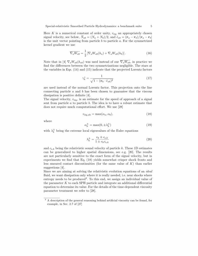
4.1 Test 1: Riemann problem 1
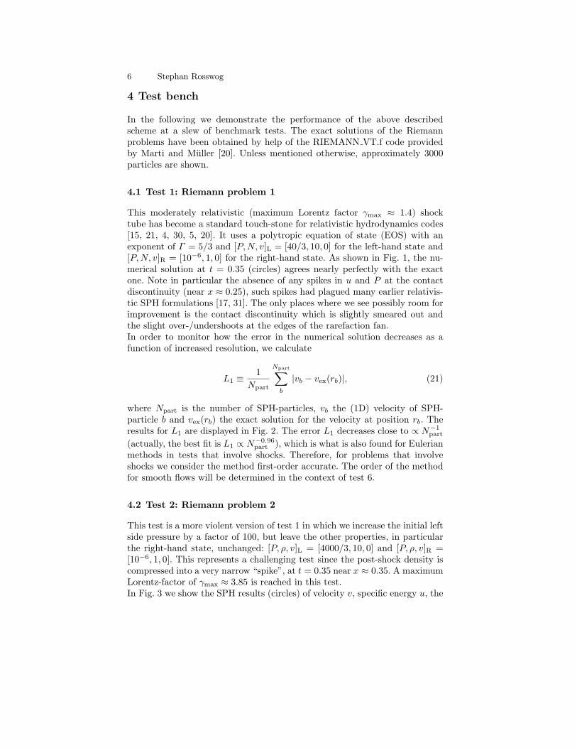
This moderately relativistic (maximum Lorentz factor γmax ≈ 1.4) shocktube has become a standard touch-stone for relativistic hydrodynamics codes[15, 21, 4, 30, 5, 20]. It uses a polytropic equation of state (EOS) with anexponent of Γ = 5/3 and [P,N, v]L = [40/3, 10, 0] for the left-hand state and[P,N, v]R = [10−6, 1, 0] for the right-hand state. As shown in Fig. 1, the nu-merical solution at t = 0.35 (circles) agrees nearly perfectly with the exactone. Note in particular the absence of any spikes in u and P at the contactdiscontinuity (near x ≈ 0.25), such spikes had plagued many earlier relativis-tic SPH formulations [17, 31]. The only places where we see possibly room forimprovement is the contact discontinuity which is slightly smeared out andthe slight over-/undershoots at the edges of the rarefaction fan.In order to monitor how the error in the numerical solution decreases as afunction of increased resolution, we calculate
L1 ≡1
Npart
Npart∑b
|vb − vex(rb)|, (21)
where Npart is the number of SPH-particles, vb the (1D) velocity of SPH-particle b and vex(rb) the exact solution for the velocity at position rb. Theresults for L1 are displayed in Fig. 2. The error L1 decreases close to ∝ N−1
part
(actually, the best fit is L1 ∝ N−0.96part ), which is what is also found for Eulerian
methods in tests that involve shocks. Therefore, for problems that involveshocks we consider the method first-order accurate. The order of the methodfor smooth flows will be determined in the context of test 6.
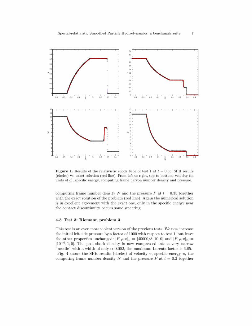
4.2 Test 2: Riemann problem 2
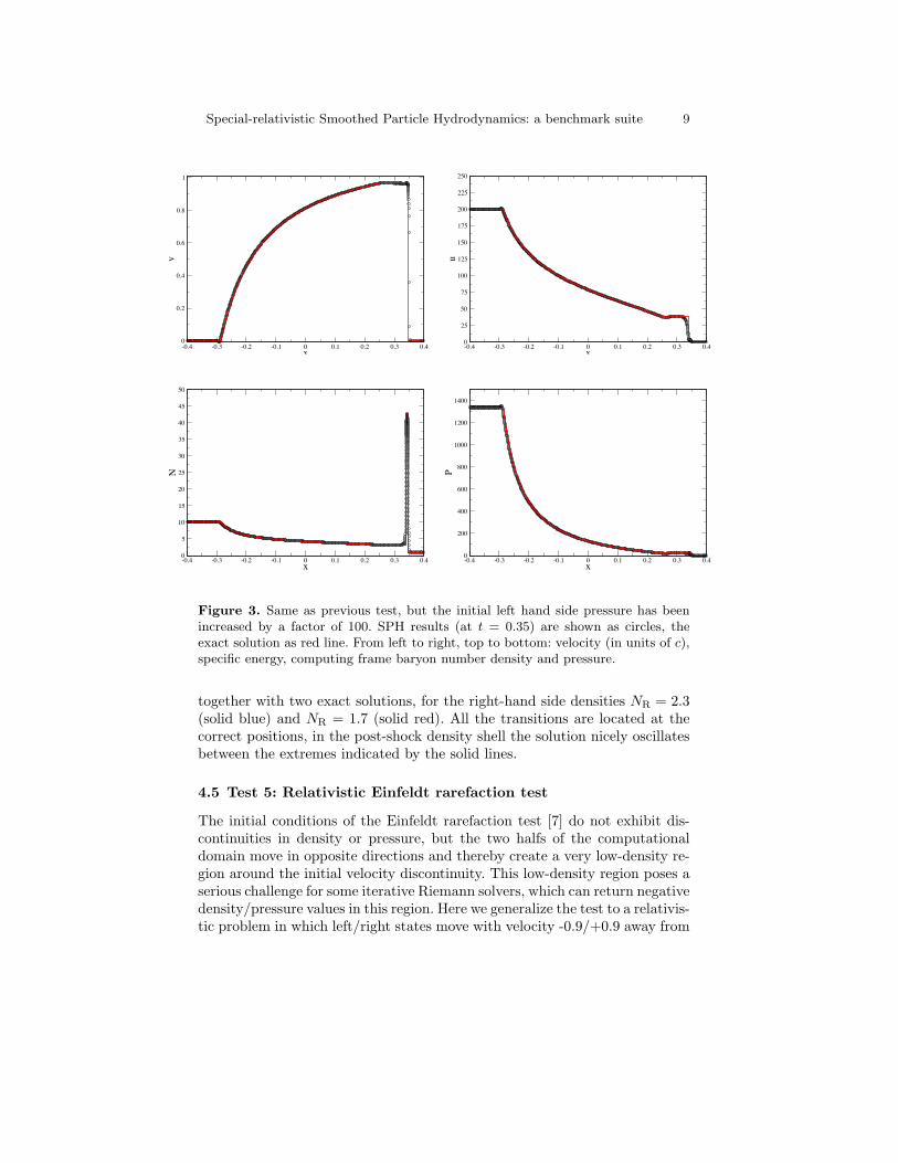
This test is a more violent version of test 1 in which we increase the initial leftside pressure by a factor of 100, but leave the other properties, in particularthe right-hand state, unchanged: [P, ρ, v]L = [4000/3, 10, 0] and [P, ρ, v]R =[10−6, 1, 0]. This represents a challenging test since the post-shock density iscompressed into a very narrow “spike”, at t = 0.35 near x ≈ 0.35. A maximumLorentz-factor of γmax ≈ 3.85 is reached in this test.In Fig. 3 we show the SPH results (circles) of velocity v, specific energy u, the
Special-relativistic Smoothed Particle Hydrodynamics: a benchmark suite 7
-0.4 -0.3 -0.2 -0.1 0 0.1 0.2 0.3 0.4x
0
0.1
0.2
0.3
0.4
0.5
0.6
0.7
0.8
0.9v
-0.4 -0.3 -0.2 -0.1 0 0.1 0.2 0.3 0.4x
0
0.2
0.4
0.6
0.8
1
1.2
1.4
1.6
1.8
2
2.2
2.4
u
-0.4 -0.3 -0.2 -0.1 0 0.1 0.2 0.3 0.4x
0
1
2
3
4
5
6
7
8
9
10
11
12
N
-0.4 -0.3 -0.2 -0.1 0 0.1 0.2 0.3 0.4x
0123456
789101112131415
P
Figure 1. Results of the relativistic shock tube of test 1 at t = 0.35: SPH results(circles) vs. exact solution (red line). From left to right, top to bottom: velocity (inunits of c), specific energy, computing frame baryon number density and pressure.
computing frame number density N and the pressure P at t = 0.35 togetherwith the exact solution of the problem (red line). Again the numerical solutionis in excellent agreement with the exact one, only in the specific energy nearthe contact discontinuity occurs some smearing.
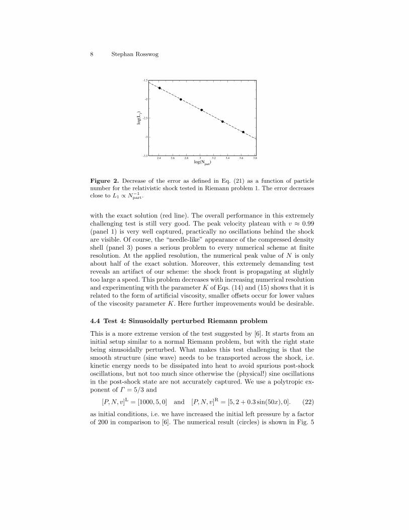
4.3 Test 3: Riemann problem 3
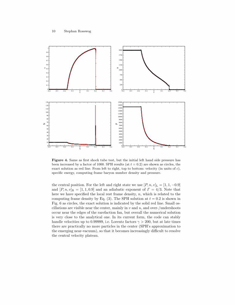
This test is an even more violent version of the previous tests. We now increasethe initial left side pressure by a factor of 1000 with respect to test 1, but leavethe other properties unchanged: [P, ρ, v]L = [40000/3, 10, 0] and [P, ρ, v]R =[10−6, 1, 0]. The post-shock density is now compressed into a very narrow“needle” with a width of only ≈ 0.002, the maximum Lorentz factor is 6.65.Fig. 4 shows the SPH results (circles) of velocity v, specific energy u, the
computing frame number density N and the pressure P at t = 0.2 together
8 Stephan Rosswog
2.4 2.6 2.8 3 3.2 3.4 3.6 3.8log(Npart)
-3.5
-3
-2.5
-2
-1.5
log(L 1)
Figure 2. Decrease of the error as defined in Eq. (21) as a function of particlenumber for the relativistic shock tested in Riemann problem 1. The error decreasesclose to L1 ∝ N−1
part.
with the exact solution (red line). The overall performance in this extremelychallenging test is still very good. The peak velocity plateau with v ≈ 0.99(panel 1) is very well captured, practically no oscillations behind the shockare visible. Of course, the “needle-like” appearance of the compressed densityshell (panel 3) poses a serious problem to every numerical scheme at finiteresolution. At the applied resolution, the numerical peak value of N is onlyabout half of the exact solution. Moreover, this extremely demanding testreveals an artifact of our scheme: the shock front is propagating at slightlytoo large a speed. This problem decreases with increasing numerical resolutionand experimenting with the parameter K of Eqs. (14) and (15) shows that it isrelated to the form of artificial viscosity, smaller offsets occur for lower valuesof the viscosity parameter K. Here further improvements would be desirable.
4.4 Test 4: Sinusoidally perturbed Riemann problem
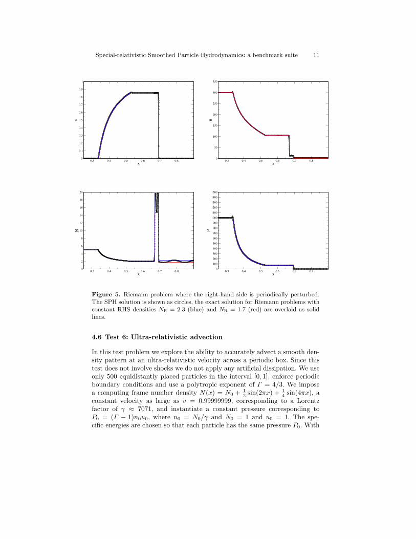
This is a more extreme version of the test suggested by [6]. It starts from aninitial setup similar to a normal Riemann problem, but with the right statebeing sinusoidally perturbed. What makes this test challenging is that thesmooth structure (sine wave) needs to be transported across the shock, i.e.kinetic energy needs to be dissipated into heat to avoid spurious post-shockoscillations, but not too much since otherwise the (physical!) sine oscillationsin the post-shock state are not accurately captured. We use a polytropic ex-ponent of Γ = 5/3 and
[P,N, v]L = [1000, 5, 0] and [P,N, v]R = [5, 2 + 0.3 sin(50x), 0]. (22)
as initial conditions, i.e. we have increased the initial left pressure by a factorof 200 in comparison to [6]. The numerical result (circles) is shown in Fig. 5
Special-relativistic Smoothed Particle Hydrodynamics: a benchmark suite 9
-0.4 -0.3 -0.2 -0.1 0 0.1 0.2 0.3 0.4x
0
0.2
0.4
0.6
0.8
1v
-0.4 -0.3 -0.2 -0.1 0 0.1 0.2 0.3 0.4x
0
25
50
75
100
125
150
175
200
225
250
u
-0.4 -0.3 -0.2 -0.1 0 0.1 0.2 0.3 0.4x
0
5
10
15
20
25
30
35
40
45
50
N
-0.4 -0.3 -0.2 -0.1 0 0.1 0.2 0.3 0.4x
0
200
400
600
800
1000
1200
1400
P
Figure 3. Same as previous test, but the initial left hand side pressure has beenincreased by a factor of 100. SPH results (at t = 0.35) are shown as circles, theexact solution as red line. From left to right, top to bottom: velocity (in units of c),specific energy, computing frame baryon number density and pressure.
together with two exact solutions, for the right-hand side densities NR = 2.3(solid blue) and NR = 1.7 (solid red). All the transitions are located at thecorrect positions, in the post-shock density shell the solution nicely oscillatesbetween the extremes indicated by the solid lines.
4.5 Test 5: Relativistic Einfeldt rarefaction test
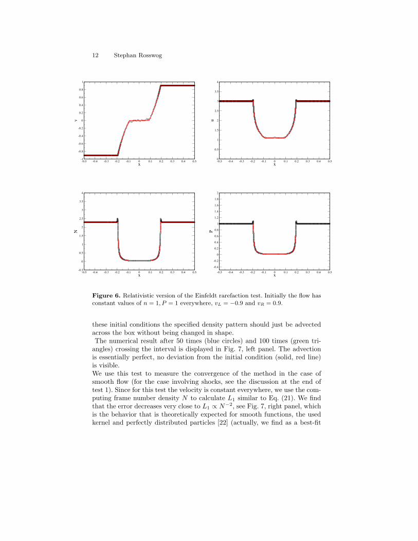
The initial conditions of the Einfeldt rarefaction test [7] do not exhibit dis-continuities in density or pressure, but the two halfs of the computationaldomain move in opposite directions and thereby create a very low-density re-gion around the initial velocity discontinuity. This low-density region poses aserious challenge for some iterative Riemann solvers, which can return negativedensity/pressure values in this region. Here we generalize the test to a relativis-tic problem in which left/right states move with velocity -0.9/+0.9 away from
10 Stephan Rosswog
-0.4 -0.3 -0.2 -0.1 0 0.1 0.2 0.3 0.4x
0
0.1
0.2
0.3
0.4
0.5
0.6
0.7
0.8
0.9
1
v
-0.4 -0.3 -0.2 -0.1 0 0.1 0.2 0.3 0.4x
0
250
500
750
1000
1250
1500
1750
2000
u
-0.4 -0.3 -0.2 -0.1 0 0.1 0.2 0.3 0.4x
0
10
20
30
40
50
60
70
80
90
100
110
120
130
N
-0.4 -0.3 -0.2 -0.1 0 0.1 0.2 0.3 0.4x
0100020003000400050006000
70008000
9000100001100012000130001400015000
P
Figure 4. Same as first shock tube test, but the initial left hand side pressure hasbeen increased by a factor of 1000. SPH results (at t = 0.2) are shown as circles, theexact solution as red line. From left to right, top to bottom: velocity (in units of c),specific energy, computing frame baryon number density and pressure.
the central position. For the left and right state we use [P, n, v]L = [1, 1,−0.9]and [P, n, v]R = [1, 1, 0.9] and an adiabatic exponent of Γ = 4/3. Note thathere we have specified the local rest frame density, n, which is related to thecomputing frame density by Eq. (3). The SPH solution at t = 0.2 is shown inFig. 6 as circles, the exact solution is indicated by the solid red line. Small os-cillations are visible near the center, mainly in v and u, and over-/undershootsoccur near the edges of the rarefaction fan, but overall the numerical solutionis very close to the analytical one. In its current form, the code can stablyhandle velocities up to 0.99999, i.e. Lorentz factors γ > 200, but at late timesthere are practically no more particles in the center (SPH’s approximation tothe emerging near-vacuum), so that it becomes increasingly difficult to resolvethe central velocity plateau.
Special-relativistic Smoothed Particle Hydrodynamics: a benchmark suite 11
0.3 0.4 0.5 0.6 0.7 0.8x
0
0.1
0.2
0.3
0.4
0.5
0.6
0.7
0.8
0.9
1
v
0.3 0.4 0.5 0.6 0.7 0.8x
0
50
100
150
200
250
300
350
u
0.3 0.4 0.5 0.6 0.7 0.8x
0
2
4
6
8
10
12
14
16
18
20
N
0.3 0.4 0.5 0.6 0.7 0.8x
0100200300400500600
700800
900100011001200130014001500
P
Figure 5. Riemann problem where the right-hand side is periodically perturbed.The SPH solution is shown as circles, the exact solution for Riemann problems withconstant RHS densities NR = 2.3 (blue) and NR = 1.7 (red) are overlaid as solidlines.
4.6 Test 6: Ultra-relativistic advection
In this test problem we explore the ability to accurately advect a smooth den-sity pattern at an ultra-relativistic velocity across a periodic box. Since thistest does not involve shocks we do not apply any artificial dissipation. We useonly 500 equidistantly placed particles in the interval [0, 1], enforce periodicboundary conditions and use a polytropic exponent of Γ = 4/3. We imposea computing frame number density N(x) = N0 + 1
2 sin(2πx) + 14 sin(4πx), a
constant velocity as large as v = 0.99999999, corresponding to a Lorentzfactor of γ ≈ 7071, and instantiate a constant pressure corresponding toP0 = (Γ − 1)n0u0, where n0 = N0/γ and N0 = 1 and u0 = 1. The spe-cific energies are chosen so that each particle has the same pressure P0. With
12 Stephan Rosswog
-0.5 -0.4 -0.3 -0.2 -0.1 0 0.1 0.2 0.3 0.4 0.5x
-1
-0.8
-0.6
-0.4
-0.2
0
0.2
0.4
0.6
0.8
1
v
-0.5 -0.4 -0.3 -0.2 -0.1 0 0.1 0.2 0.3 0.4 0.5x
0
0.5
1
1.5
2
2.5
3
3.5
4
u
-0.5 -0.4 -0.3 -0.2 -0.1 0 0.1 0.2 0.3 0.4 0.5x
-0.5
0
0.5
1
1.5
2
2.5
3
3.5
4
N
-0.5 -0.4 -0.3 -0.2 -0.1 0 0.1 0.2 0.3 0.4 0.5x
-0.4
-0.2
0
0.2
0.4
0.6
0.8
1
1.2
1.4
1.6
1.8
2
P
Figure 6. Relativistic version of the Einfeldt rarefaction test. Initially the flow hasconstant values of n = 1, P = 1 everywhere, vL = −0.9 and vR = 0.9.
these initial conditions the specified density pattern should just be advectedacross the box without being changed in shape.The numerical result after 50 times (blue circles) and 100 times (green tri-
angles) crossing the interval is displayed in Fig. 7, left panel. The advectionis essentially perfect, no deviation from the initial condition (solid, red line)is visible.We use this test to measure the convergence of the method in the case ofsmooth flow (for the case involving shocks, see the discussion at the end oftest 1). Since for this test the velocity is constant everywhere, we use the com-puting frame number density N to calculate L1 similar to Eq. (21). We findthat the error decreases very close to L1 ∝ N−2, see Fig. 7, right panel, whichis the behavior that is theoretically expected for smooth functions, the usedkernel and perfectly distributed particles [22] (actually, we find as a best-fit

Special-relativistic Smoothed Particle Hydrodynamics: a benchmark suite 13
0 0.1 0.2 0.3 0.4 0.5 0.6 0.7 0.8 0.9 1x
0.4
0.6
0.8
1
1.2
1.4
1.6
N
after 100 intervall crossingsafter 50 intervall crossingsinitial condition
v= 0.99999999! = 7071
2 2.2 2.4 2.6 2.8 3log(Npart)
-5
-4.5
-4
-3.5
-3
log(L 1)
Figure 7. Left: Ultra-relativistic advection (v = 0.99999999, Lorentz factor γ =7071) of a density pattern across a periodic box. The advection is essentially perfect,the patterns after 50 (blue circles) and 100 (green triangles) times crossing the boxare virtually identical to the initial condition (red line). Right: Decrease of theL1 error as a function of resolution, for smooth flows the method is second-orderaccurate.
exponent -2.07). Therefore, we consider the method second-order accurate forsmooth flows.
5 Conclusions
We have summarized a new special-relativistic SPH formulation that is de-rived from the Lagrangian of an ideal fluid [28]. As numerical variables it usesthe canonical energy and momentum per baryon whose evolution equationsfollow stringently from the Euler-Lagrange equations. We have further appliedthe special-relativistic generalizations of the so-called “grad-h-terms” and arefined artificial viscosity scheme with time dependent parameters.The main focus of this paper is the presentation of a set of challenging bench-mark tests that complement those of the original paper [28]. They show theexcellent advection properties of the method, but also its ability to accuratelyhandle even very strong relativistic shocks. In the extreme shock tube test 3,where the post-shock density shell is compressed into a width of only 0.1 %of the computational domain, we find the shock front to propagate at slightlytoo large a pace. This artifact ceases with increasing numerical resolution, butfuture improvements of this point would be desirable. We have further deter-
14 Stephan Rosswog
mined the convergence rate of the method in numerical experiments and findit first-order accurate when shocks are involved and second-order accurate forsmooth flows.
References
1. S. Ayal, T. Piran, R. Oechslin, M. B. Davies, and S. Rosswog, Post-NewtonianSmoothed Particle Hydrodynamics, ApJ 550 (2001), 846–859.
2. T. W. Baumgarte and S. L. Shapiro, Numerical Relativity and Compact Bina-ries, Phys. Rep. 376 (2003), 41–131.
3. A. Bauswein, R. Oechslin, and H. -J. Janka, Discriminating Strange Star Merg-ers from Neutron Star Mergers by Gravitational-Wave Measurements, ArXive-prints (2009).
4. J. E. Chow and J.J. Monaghan, Ultrarelativistic SPH, J. Computat. Phys. 134(1997), 296.
5. L. Del Zanna and N. Bucciantini, An Efficient Shock-capturing Central-typeScheme for Multidimensional Relativistic Flows. I. Hydrodynamics, A&A 390(2002), 1177–1186.
6. A. Dolezal and S. S. M. Wong, Relativistic Hydrodynamics and Essentially Non-oscillatory Shock Capturing Schemes, J. Comp. Phys. 120 (1995), 266.
7. B. Einfeldt, P. L. Roe, C. D. Munz, and B. Sjogreen, On Godunov-type MethodsNear Low Densities, J. Comput. Phys. 92 (1991), 273–295.
8. J. A. Faber, T. W. Baumgarte, S. L. Shapiro, K. Taniguchi, and F. A. Rasio,Dynamical Evolution of Black Hole-Neutron Star Binaries in General Relativity:Simulations of Tidal Disruption, Phys. Rev. D 73 (2006), no. 2, 024012.
9. J. A. Faber, P. Grandclement, and F. A. Rasio, Mergers of Irrotational NeutronStar Binaries in Conformally Flat Gravity, Phys. Rev. D 69 (2004), no. 12,124036.
10. J. A. Faber and F. A. Rasio, Post-Newtonian SPH Calculations of Binary Neu-tron Star Coalescence: Method and First Results, Phys. Rev. D 62 (2000), no. 6,064012.
11. J. A. Faber and F. A. Rasio, Post-Newtonian SPH Calculations of Binary Neu-tron Ntar Coalescence. III. Irrotational Systems and Gravitational Wave Spec-tra, Phys. Rev. D 65 (2002), no. 8, 084042.
12. J. A. Faber, F. A. Rasio, and J. B. Manor, Post-Newtonian Smoothed ParticleHydrodynamics Calculations of Binary Neutron Star Coalescence. II. BinaryMass Ratio, Equation of State, and Spin Dependence, Phys. Rev. D 63 (2001),no. 4, 044012.
13. V. Fock, Theory of Space, Time and Gravitation, Pergamon, Oxford, 1964.14. J. Font, Numerical Hydrodynamics in General Relativity, Living Rev. Relativ.
3 (2000), 2.15. J. F. Hawley, L. L. Smarr, and J. R. Wilson, A Numerical Study of Nonspherical
Black Hole Accretion. II - Finite Differencing and Code Calibration, ApJS 55(1984), 211–246.
16. A. Kheyfets, W. A. Miller, and W. H. Zurek, Covariant Smoothed Particle Hy-drodynamics on a Curved Background, Phys. Rev. D 41 (1990), 451–454.
17. P. Laguna, W. A. Miller, and W. H. Zurek, Smoothed Particle HydrodynamicsNear a Black Hole, ApJ 404 (1993), 678–685.
Special-relativistic Smoothed Particle Hydrodynamics: a benchmark suite 15
18. P.J. Mann, A Relativistic Smoothed Particle Hydrodynamics Method Tested withthe Shock Tube, Comp. Phys. Commun. (1991).
19. P.J. Mann, Smoothed Particle Hydrodynamics Applied to Relativistic SphericalCollapse, J. Comput. Phys. 107 (1993), 188–198.
20. J. M. Marti and E. Muller, Numerical Hydrodynamics in Special Relativity,Living Rev. Relativ. 6 (2003), 7.
21. J.M. Marti and E. Muller, Extension of the Piecewise Parabolic Method to One-Dimensional Relativistic Hydrodynamics, J. Comp. Phys. 123 (1996), 1.
22. J. J. Monaghan, Smoothed Particle Hydrodynamics, Ann. Rev. Astron. Astro-phys. 30 (1992), 543.
23. J. J. Monaghan, SPH Compressible Turbulence, MNRAS 335 (2002), 843–852.24. J. J. Monaghan, Smoothed Particle Hydrodynamics, Rep. Prog. Phys. 68 (2005),
1703–1759.25. J. J. Monaghan and D. J. Price, Variational Principles for Relativistic Smoothed
Particle Hydrodynamics, MNRAS 328 (2001), 381–392.26. R. Oechslin, S. Rosswog, and F.-K. Thielemann, Conformally Flat Smoothed
Particle Hydrodynamics Application to Neutron Star Mergers, Phys. Rev. D 65(2002), no. 10, 103005.
27. S. Rosswog, Astrophysical Smooth Particle Hydrodynamics, New Astron. Rev.53 (2009), 78.
28. S. Rosswog, Conservative, Special-relativistic Smooth Particle Hydrodynamics,submitted to J. Comp. Phys. (2009), eprint arXiv:0907.4890.
29. S. Rosswog, Relativistic Smooth Particle Hydrodynamics on a Given BackgroundSpace-time, Classical Quantum Gravity, in press (2010).
30. S. Siegler, Entwicklung und Untersuchung eines Smoothed Particle Hydrody-namics Verfahrens fur relativistische Stromungen, Ph.D. thesis, Eberhard-Karls-Universitat Tubingen, 2000.
31. S. Siegler and H. Riffert, Smoothed Particle Hydrodynamics Simulations of Ul-trarelativistic Shocks with Artificial Viscosity, ApJ 531 (2000), 1053–1066.
32. V. Springel and L. Hernquist, Cosmological Smoothed Particle HydrodynamicsSimulations: the Entropy Equation, MNRAS 333 (2002), 649–664.