speciation, sources and bioavailability of copper … sources and bioavailability of copper and zinc...

Speciation, Sources and Bioavailability of

Copper and Zinc in

DoD-Impacted Harbors and Estuaries

Project Final Report February 2005

CP 1158 (Updated March 2007)

Martin Shafer Ph.D., Degui Tang Ph.D., Jocelyn Hemming Ph.D., Brian Beard Ph.D., David Armstrong Ph.D. Environmental Chemistry and Technology

University of Wisconsin-Madison February 2005

Distribution Statement A: Approved for Public Release, Distribution is Unlimited

This report was prepared under contract to the Department of Defense Strategic Environmental Research and Development Program (SERDP). The publication of this report does not indicate endorsement by the Department of Defense, nor should the contents be construed as reflecting the official policy or position of the Department of Defense. Reference herein to any specific commercial product, process, or service by trade name, trademark, manufacturer, or otherwise, does not necessarily constitute or imply its endorsement, recommendation, or favoring by the Department of Defense.

2

Page 2 of 79

Contents I. Introduction & Synopsis . . . . . . . . . . . . . . . . . . . . . . . . . . . . . . . . . . 03 II. Manuscripts Published in Peer-Reviewed Journals . . . . . . . . . 08 III. Selected Presentations Given at International Meetings . . . . . 14 IV. Theses Defended . . . . . . . . . . . . . . . . . . . . . . . . . . . . . . . . . . 14 V. Field Campaigns. . . . . . . . . . . . . . . . . . . . . . . . . . . . . . . . . . . . 15 A. Study Sites . . . . . . . . . . . . . . . . . . . . . . . . . . . . . . . . . . . . . 15 B. Field Operations Summary . . . . . . . . . . . . . . . . . . . . . . . . . 20 VI. Speciation Studies . . . . . . . . . . . . . . . . . . . . . . . . . . . . . . . . . . 23

A. Summary . . . . . . . . . . . . . . . . . . . . . . . . . . . . . . . . . . . . . . 23 B. Cape Fear. . . . . . . . . . . . . . . . . . . . . . . . . . . . . . . . . . . . . . 24 C. Norfolk-Hampton Roads . . . . . . . . . . . . . . . . . . . . . . . . . . 29 D. San Diego Bay . . . . . . . . . . . . . . . . . . . . . . . . . . . . . . . . . . 33 E. Filterable Copper – Strong Ligand Comparison . . . . . . . . 39 F. Chelex Lability Summary . . . . . . . . . . . . . . . . . . . . . . . . . . 40

VII. Ligand & Dissolved Organic Matter Character . . . . . . . . . . . . . 42 VIII. Copper & Zinc Partitioning. . .. . . . . . . . . . . . . . . . . . . . . . . . . . 46 IX. Thiol Ligand Production & Excretion . . . . . . . . . . . . . . . . . . . . . 51 X. Bioavailability Studies . . . . . . . . . . . . . . . . . . . . . . . . . . . . . . . . 55 A. Bioassay Protocols . . . . . . . . . . . . . . . . . . . . . . . . . . . . . . 55 B. Selected Outcomes . . . . . . . . . . . . . . . . . . . . . . . . . . . . . . 60 XI. Copper Stable Isotope Ratio Studies . . . . . . . . . . . . . . . . . . . . 67

A. Goal and Summary . . . . . . . . . . . . . . . . . . . . . . . . . . . . . . 67 B. Background and Theory . . . . . . . . . . . . . . . . . . . . . . . . . . 69 C. Analytical Considerations . . . . . . . . . . . . . . . . . . . . . . . . . 71 D. Analytical Progress . . . . . . . . . . . . . . . . . . . . . . . . . . . . . . 72 E. Samples for Stable Isotope Ratio Analysis . . . . . . . . . . . . 75

3

Page 3 of 79

I. Introduction & Synopsis The response of organisms to metal exposure is dependent on the chemical and physical associations (speciation) as well as the concentration of the respective metal. Metal toxicity is regulated by the biogeochemical environment in which it exists, with the metals physical form, kinetic lability, and oxidation state mediating bioavailability. With few exceptions, the uptake rate of a trace metal by an organism is largely dependent on its “free” or hydrated concentration in the growth environment. The “free” or available metal is regulated by a complex series of competition reactions among aqueous ligands and cell membrane-associated ligands that transport metals into the organism (Figure 1). Therefore total and operationally defined “dissolved” metal concentrations are not necessarily predictive of toxicity or potential risk to the environment. Current regulatory frameworks and metrics do not adequately address metal speciation and addressing speciation will enable more realistic estimations of acute and chronic risk from metal exposures. The overarching goal of this SERDP project was to advance our understanding of metal-ligand binding in order to further the development of practical and predictive models of trace metal bioavailability. This goal is illustrated in Figure 2. Our primary speciation focus was on Strong Metal-Binding Ligands and Colloidal Phases. Figure 1. Copper speciation in aquatic environments. (modified from Turner 1995)

Cu(I) e.g. CuCl2-

dissolvedinorganic

complexes

dissolvedorganic

complexes

Cu-fulvicCu-humic

complexes

adsorbedCu

Cu inorganisms

Cu2+

DISSOLVED

COLLOIDAL

PARTICULATE

reduction

complexation

complexation

biologicalavailability

geochemicalavailability

4

Page 4 of 79

Total Metal

LabileSpeciesbyChemical +PhysicalSpeciation

AvailableSpecies

byBioassay

Measures

PredictiveToolsFor

-Bioavailability-Toxicity

Figure 2. Develop Practical Speciation Procedures, with Bioassay Grounding for the Prediction of Bioavailable Forms of Metals.

In this project we isolated important metal-ligand pools and characterized the ligands and their metal-binding properties in three contrasting marine estuaries, focusing primarily on Copper (Cu) and to a lesser degree, Zinc (Zn). Chemical measures of metal speciation were linked to bioavailability as quantified in parallel laboratory studies with marine algae. Multiple bioavailability/toxicity endpoints including: (1) cellular budgets of trace metals, (2) molecular biomarkers, and (3) growth characteristics, were measured. Rigorous trace metal “clean” protocols (Figure 4) were integrated throughout all components of the study, including the bioassay studies, and state-of-the-art analytical techniques were applied for speciation measurements. Our chemical speciation tools included electrochemical methods (Figure 6), principally voltammetry (Cathodic Stripping Voltammetry (CSV) and Anodic Stripping Voltammetry (ASV)), and kinetic separations on chelating-resins. Ultrafiltration (Figure 5) at 1 kDa and 10 kDa was also routinely applied to fractionate aquatic ligand pools. For our study systems, we chose three DoD-impacted marine estuaries with major contrasts in ligand source, type, and abundance, as well as significant gradients in trace element levels. These are: (a) San Diego Bay, California, (b) Norfolk Harbor, Virginia, and (c) Cape Fear, North Carolina. The overall approach is diagramed in Figure 3.

5

Page 5 of 79

Figure 3. Project Approach.

Extensive field studies documented the existence of large gradients in metal speciation, both between and within systems. In San Diego Bay, levels of strong ligand [L1] increase markedly from North to South Bay, however, in general concentrations of [L1] and Cu are similar. In both the Cape Fear and Norfolk systems, levels of strong ligand are in large excess of Cu levels; (e.g. [L1] = 10x [Cu]), and “free” Cu levels are therefore extremely low (pCu = 14-15). Significant differences in the “quality” of the organic matter are apparent, as shown by large contrasts in normalized Cu-binding ligand levels. Colloidal phases of Cu and DOM were significant, if not the dominant, pools in each of the study systems, particularly at sites with high algal production or where there are large inputs of terrestrial carbon. Cu-binding ligands are also predominantly found in the colloidal size fraction, and in both colloidal and dissolved phases, represent only a very small fraction of DOM mass. Kinetic separations on Chelex resin revealed the presence of large non-labile pools of

POTW

Harbor

Fractionation / Speciation

SourceApportionment

Bioavailability

Ultrafiltration DEAEChelex

Uptake Growth Rate Biochemical

Characterization

StableIsotopeAnalysis

Parameterizationof Metal

Association

IsotopeSpike

IsotopeSpike

Voltammetry

Isotope Partitioning

Chelex Kinetics

Trace Metals

Filtration

WatershedIndustrial

DoDSources

Collaboration withand Support for

Skrabal and Zirino

Ligands-chemical

composition-size/shape-functional

group-aromaticity

-bindingcapactity-stability

6

Page 6 of 79

Cu in each of the study systems, and a close relationship was observed between colloidal and non-labile species. In contrast to Cu, a super-majority of filterable Zn in each system was labile to Chelex. Copper partitioning to colloids is significantly greater than that to particles. Bioavailability studies indicated that Cu uptake into cells can be accurately predicted from levels of strong ligand [L1]. The fraction of filterable Cu bioavailable is greatest in the San Diego system. Bioavailability is greatly enhanced by ultrafiltration, where up to 75% of ambient Cu is accessible after ligand level reduction. These results strongly support efforts to develop speciation-based water quality criteria. The technology and models underpinning these findings should be transferable to scientists within EPA and DoD.

Figure 4. Trace metal “clean” sampling in San Diego Bay.

7

Page 7 of 79

Figure 5. Ultrafiltration of Cape Fear estuarine water.

Figure 6. Cathodic stripping voltammetry.

Permeates Concentrates<0.4 µm <10 kD <1 kD >1 kD >10 kD



8

Page 8 of 79

II. Manuscripts Published in Peer-Reviewed Journals The following research manuscripts, all published in high-impact factor peer-reviewed journals, were produced exclusively from data developed over the course of this study. SERDP was clearly acknowledged as the funding agency in each manuscript. A brief summary of our findings is presented after each manuscript abstract. The full manuscripts are provided in the Appendix to this report.

1. Tang, D., K. Vang, D.A. Karner, D.A. Armstrong, and M.M. Shafer. 2003. Determination of Dissolved Thiols Using Solid Phase Extraction and HPLC Analysis of Fluorescently Derivatized Thiolic Compounds. Journal of Chromatography A, 998(1-2):31-40.

Abstract A method employing solid-phase extraction coupled with HPLC separation of thiol-monobromobimane (mBBr) derivatives was developed and optimized to quantify dissolved thiols at concentrations as low as 0.1 nM for glutathione (GSH) and γ-glutamylcysteine (γEC) in natural waters. Careful control of the derivatization conditions is crucial for successful detection in both the direct and the solid-phase extraction measurements. The reducing reagent, tri-n-butylphosphine (TBP), is needed for complete derivatization. At the optimal addition of TBP ([TBP]/[mBBr] = 0.4–1.6). Cu, which is present at higher concentrations than thiols in most natural waters, does not interfere with the determination of thiols under these derivatization conditions. Other soft metals such as Ag(I) and Hg(II) are present at levels typically less than 10 pM in natural waters, so their effects on thiol quantification should be minimal. The thiol fluorescence signal was totally suppressed if the mole ratio of TBP to mBBr was 2.6 or greater. Consistent recovery of thiols standards in a NaCl solution (0.5 M) was obtained using the Waters HLB reversed-phase resin, and blank levels of GSH and γEC were extremely low (less than 0.03 nM). The detection limits for GSH, γEC and phytochelatin-2 (PC-2) were 0.03, 0.03, and 0.06 nM, respectively. Linear ranges for the thiols studied were excellent, typically from 0.1 to 20 nM.. This study demonstrates the capability of a new method for detection of low levels of dissolved thiols in aqueous systems using solid-phase extraction coupled with HPLC detection. The method will significantly enhance the ability to investigate the release of dissolved thiols from algae and their role in regulating trace metal bioavailability in surface.

2. Shafer, M., S. Hoffmann, J. Overdier, and D. Armstrong. 2004. Physical and kinetic speciation of Copper and Zinc in three geochemically contrasting marine estuaries. Environmental Science and Technology 38(14):3810-3819.

Abstract The physical and kinetic speciation of Cu and Zn in three impacted marine estuaries was examined. Contrasts in sources of metal-binding ligands, solution chemistry, and hydrologic

9

Page 9 of 79

forcing between and within the three study systems (Cape Fear River Estuary, North Carolina; Norfolk-Hampton Roads-Elizabeth River, Virginia; San Diego Bay, California) were exploited to enhance our understanding of Cu and Zn speciation. Trace metal-optimized tangential flow ultrafiltration at 1 kDa nominal molecular weight limit (NMWL) was used to fractionate <0.4 µm species into colloidal and “dissolved” pools. Colloidal species of dissolved organic matter (DOM) and copper were significant and often the dominant pools in each of the three study systems. Characteristic colloidal fractions of both DOM and Cu ranged from near 70% of <0.4 µm concentrations in Cape Fear to 50% in San Diego Bay. Colloidal Cu and DOM were strongly coupled, and variability in observed <0.4 µm Cu concentrations was closely related to the concentrations of colloidal-associated metal. Colloidal fractions were much smaller for Zn than that of Cu; ranging from 10-30% in Cape Fear to less than 5% in San Diego Bay, and no relationship to DOM was observed. Kinetic separations on Chelex resin revealed the presence of large non-labile pools of Cu in each of the study systems, with the highest fractions (70-100%) in Cape Fear and Norfolk and lowest (30-50%) in San Diego Bay. A close relationship was observed between colloidal and non-labile Cu species, implying slow reactivity of colloidal-bound Cu. The fraction of filterable Zn labile to Chelex averaged 97%, 85%, and 60% in San Diego, Norfolk, and Cape Fear, respectively. Anthropogenic Zn appeared almost exclusively in the <1 kDa fraction, while anthropogenic Cu was distributed between dissolved and colloidal pools. Copper particle-partition coefficients (Kd) followed the trend: San Diego >> Norfolk > Cape Fear and were inversely correlated with DOC concentrations. Colloid-based partition coefficients were significantly greater, in many cases an order of magnitude greater, than particle-based partition coefficients. The partitioning data suggest the presence of metal-enriched bacterial-derived exudates and/or discrete metal phases in colloidal-sized particles in impacted regions of these estuaries. The strong relationships observed between Cu and DOC indicates that Cu partitioning behavior over a range of estuarine environments may be modeled effectively with a limited set of coefficients. Our measurements of metal lability and size distribution imply that the fraction of <0.4 µm Zn that is likely to be bioavailable is greater than that for Cu, especially in impacted regions of the study systems.

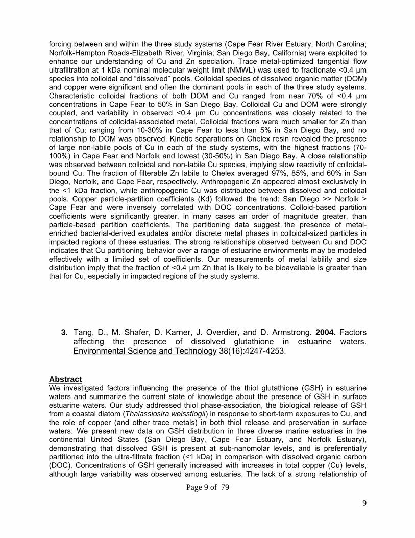
3. Tang, D., M. Shafer, D. Karner, J. Overdier, and D. Armstrong. 2004. Factors affecting the presence of dissolved glutathione in estuarine waters. Environmental Science and Technology 38(16):4247-4253.

Abstract We investigated factors influencing the presence of the thiol glutathione (GSH) in estuarine waters and summarize the current state of knowledge about the presence of GSH in surface estuarine waters. Our study addressed thiol phase-association, the biological release of GSH from a coastal diatom (Thalassiosira weissflogii) in response to short-term exposures to Cu, and the role of copper (and other trace metals) in both thiol release and preservation in surface waters. We present new data on GSH distribution in three diverse marine estuaries in the continental United States (San Diego Bay, Cape Fear Estuary, and Norfolk Estuary), demonstrating that dissolved GSH is present at sub-nanomolar levels, and is preferentially partitioned into the ultra-filtrate fraction (<1 kDa) in comparison with dissolved organic carbon (DOC). Concentrations of GSH generally increased with increases in total copper (Cu) levels, although large variability was observed among estuaries. The lack of a strong relationship of

10

Page 10 of 79

GSH concentration across systems, sites, and season to a single variable is not surprising in view of the expected influences of biota species type, other metals (e.g., Mn), and concurrent and possibly opposing effects of Cu and DOC on GSH release and preservation. In 30-h exposure experiments, release of dissolved GSH from the diatom Thalassiosira weissflogii into organic ligand-free experimental media was a strong function of added Cu concentration. The released GSH increased from about 0.02 to 0.27 fmol/cell as Cu was increased from the background level (0.5 nM) to 310 nM in the modified Aquil media. However, excretion of GSH was lower (up to 0.13 fmol/cell) when cells were grown in surface waters of San Diego Bay, despite much higher total Cu concentrations. Experiments conducted in-situ in San Diego Bay water indicated that high concentrations of added Cu destabilized GSH, while both Mn(II) and natural colloids promoted GSH stability. In contrast, laboratory experiments in synthetic media indicated that moderate levels of added Cu enhanced GSH stability. In summary, we have shown that GSH, the major low molecular weight thiol in phytoplankton, is released from phytoplankton in significant amounts and that release is enhanced by Cu. Given the observed lability of GSH in solution and our measurements documenting the presence of significant levels of GSH in natural waters, it is plausible that the dissolved species of GSH detected is the more stable disulfide form (GSSG) and/or complexed with metals. The influences of Cu on GSH stability are complex. Our experiments indicated that added Cu promoted degradation of GSH in a natural water but enhanced stability in a synthetic medium. These differences may be due to contrasts in GSH concentration, GSH/Cu ratios, and/or chemical composition of the natural water and synthetic medium. Dissolved organic matter may promote stability through conjugation or enhance degradation through photochemical reactions.

4. Tang, D., M. Shafer, D. Karner, and D. Armstrong. 2005. Response of non-protein thiols to copper stress and extracellular release of glutathione in the diatom Thalassiosira weissflogii. Limnology and Oceanography 50(2):516-525.

Abstract In this manuscript we present results from bioassay experiments using a coastal diatom, Thalassiosira weissflogii, data that document (1) the physiological response of the diatom to copper exposure in terms of photosynthetic pigments and intracellular thiols, (2) the induction and release of essential thiols from the diatom cells and the implications of these processes, and (3) comparability of cell growth and excretion of metal-complexing ligands in the metal-buffered and metal-unbuffered media. We studied the dynamic changes of cellular thiols and the extracellular release of glutathione (GSH) during growth of the marine diatom Thalassiosira weissflogii under varying levels of copper (Cu) addition in both metal buffered (with EDTA) and un-buffered (without EDTA) media. In summary, we found that, with certain exceptions, cell growth, intracellular thiol induction, and extracellular GSH release were comparable at similar Cu exposure levels in both the EDTA-buffered and un-buffered medium. These findings substantiate the premise that algae respond nearly exclusively to inorganic species of Cu. In both media, specific growth rates of greater than 1 per day were obtained at total inorganic Cu concentrations of less than 80 nmol L-1; however, at higher Cu levels, cell growth was significantly suppressed. The cell quotas of thiols and Chl a both decreased with growth time, so that Chl a–normalized cellular thiol concentrations were more or less conservative, with normalized values in the range of 0.5 and 1.5 mmol GSH (g-Chl a)-1. A clear dose–response relationship was observed between PC2:GSH ratio and inorganic Cu levels in EDTA-un-

11

Page 11 of 79

buffered medium, regardless of growth time; however, a more complicated pattern was observed in EDTA-buffered medium. GSH was released from the phytoplankton cells at generally similar concentrations into both the EDTA-buffered and un-buffered growth media—so it does not appear that the presence of a synthetic metal chelator substantially affects thiol release. GSH release was closely related to Cu-induced cell membrane damage. The extracellular GSH release rate was higher in normally grown cultures than in growth-limited cultures but lower than in growth-suppressed cultures. There is, however, an indication that EDTA possibly enhanced the release of GSH, as indicated by the higher dead:live cell ratios under EDTA-replete conditions. We also demonstrated that the release of GSH from the diatom and Cu exposure are in some sense decoupled. For normally growing cells, about 1.5–2.2% of cellular GSH is released in the early exponential growth phase and 9.2% released in the late exponential phase, with the difference likely reflecting physiological changes during growth (mainly the decrease of cellular GSH quota). At background Cu conditions (~1 nmol L-1), glutathione was excreted at an average rate of 0.087 fmol cell-1 d-1 in both media, but release increased with increasing inorganic Cu concentrations. At the elevated Cu exposures (total inorganic [Cu] 100 nmol L-1), substantially greater amounts of GSH were released, corresponding to the changes of the cell membrane integrity. The excretion of GSH apparently reflects physiological conditions during algal growth rather than an enzymatic response of the algae to control trace metal speciation in the media. Thus, the Cu-enhanced release of glutathione into ambient waters is probably an inadvertent by-product of cell membrane damage by Cu rather than a feedback mechanism to control the speciation (and toxicity) of aqueous Cu. However, at background levels of Cu, glutathione released from algae could contribute a significant portion of the Cu-complexing ligands in oceanic waters.

5. Karner, D., M. Shafer, J. Overdier, J. Hemming, and W. Sonzogni. 2006. An algal probe for copper speciation in marine waters: Lab method development. Environmental Toxicology and Chemistry 25(4):1106-1113.

Abstract The present experiments were designed to develop a laboratory-based marine algal bioassay to examine the bioavailability of Cu with minimal use of synthetic ligands, such as EDTA. Our principal research objective was to develop a robust bioassay protocol for metal speciation in marine waters using an algal probe. We wanted to minimize trace levels of EDTA in samples to avoid compromising ambient speciation but also to allow chemical speciation of metal-binding ligands excreted by the phytoplankton cells, which may be masked in the presence of EDTA. The principal focus of our experiments was on Cu; however, some experiments with Zn also were conducted (not reported here). We found that Zn toxicity was substantially lower than that of Cu and likely was irrelevant in most marine waters. The marine diatom Thalassiosira weissflogii was employed as our bioassay test organism. The first goal of the present experiments was to determine the optimal assay length, temperature, and light conditions resulting in optimal Cu concentration responses. The second goal was to determine if algal growth could be successfully maintained when EDTA, Cu, and Zn were removed from the experimental media. The final goal was to establish if robust Cu concentration responses could be achieved without EDTA buffering.

12

Page 12 of 79

Laboratory-based algal assays were developed to explore the bioavailability of copper to the marine alga Thalassiosira weissflogii. The assay was shown to be both reliable and reproducible to increasing levels of Cu. Growth consistently decreased as total Cu increased to 340 nM, with a significant reduction in growth occurring at total Cu levels of 100 nM or greater. A calibration strategy was developed that avoided use of the synthetic ligand ethylenediaminetetraacetic acid (EDTA) in the Aquil growth medium, thereby allowing ambient metal speciation. In a comparison of T. weissflogii cells grown in Aquil medium with EDTA to medium containing no added copper, zinc, and less than 0.003 nM of EDTA, no significant growth differences were observed after 8 d, indicating adequate stored nutrients. A 30-h assay was selected as the optimal time frame after examination of data from concentration–response experiments. Using 65Cu stable isotope additions, parameters examined included growth, chlorophyll a, copper uptake, phytochelatin production, and dissolved organic carbon excretion. The T. weissflogii specific growth rates decreased from 1.36 d-1 at pCu (i.e., the negative logarithmic concentration of free Cu) = 8.8 to 0.56 d-1 at pCu = 7.8, whereas intercellular copper concentrations increased from 13.6 to 70.1 fg/cell, respectively. Calculated values of the copper concentration that caused a 50% reduction in algal growth of pCu = 7.7 and copper per algal mass of 625 µg/g were established. Using an algal assay based on EDTA-free culture medium, along with trace-metal clean techniques, the effect of copper on T.weissflogii and the speciation of copper in marine waters can be studied. The method described has been applied to contrasting marine–estuarine environments, and the results from these studies will be presented in follow-up papers. The elimination of EDTA from growth media such as Aquil has the potential to improve phytoplankton–trace metal interaction studies in several important areas. Its removal not only eliminates direct algal cell toxicity associated with high concentrations of EDTA but also EDTA-enhanced release of glutathione, an antioxidant and primary precursor to phytochelatin production. The presence of EDTA severely compromises phytoplankton studies addressing intra- and extracellular complexation of metals by competing with algal-produced - excreted ligands (e.g., thiols, phytochelatins) for the target metals. The presence of EDTA in Aquil also can bind essential metals required by phytoplankton. As demonstrated in the present study, use of a large excess of EDTA in the Cu-spike solution to achieve low free Cu levels may have the unintended consequence of binding other essential trace metals, such as Zn, and decreasing them to a level at which growth is suppressed. A recent study demonstrated that high concentrations of EDTA can change the speciation of Fe and also raise organic carbon levels; therefore, the use of EDTA was not recommended when studying Fe limitation in phytoplankton. For many metals of concern, effective control of free metal-ion levels over a wide concentration range is difficult to achieve with EDTA, and use of alternative synthetic chelators can be equally (or more) problematic. Although use of synthetic ligands to control free ion levels in metal-bioassay experiments has its place, the present study and other recent investigations demonstrate that the use of EDTA is not necessary and may even be problematic. By applying innovative trace-metal clean methods, use of EDTA in trace-metal bioassay experiments can be avoided.

13

Page 13 of 79

6. Karner, D., M. Shafer, J. Overdier, J. Hemming, and W. Sonzogni. 2007. Roles

of dissolved and colloidal DOC in regulating copper toxicity to the marine alga Thalassiosira weissflogii. In review at: Environmental Toxicology and Chemistry.

Abstract The specific influence of colloidal (1 kDa – 0.4 µm) and dissolved (< 1 kDa) natural organic matter (NOM) on copper (Cu) bioavailability and toxicity to the marine alga Thalassiosira weissflogii was evaluated in water samples collected from three estuaries: Cape Fear, NC; Norfolk, VA; and San Diego, CA (USA). Trace metal clean filtration and ultrafiltration techniques were employed to separate samples into the < 0.4 µm and < 1 kDa fractions (colloid-free) used in 30 h bioassay titrations with 65Cu additions. Bioavailability was determined by measuring the cellular Cu quota, whereas toxicity was indicated by a reduction in the specific growth rate SGR). With increasing Cu concentrations, the specific growth rates generally decreased (controls with no added Cu averaged 1.23 and 1.22 d-1 for < 0.4 µm and < 1 kDa fractions, respectively; decreasing to 0.70 and 0.45 d-1, respectively, at highest Cu additions) and cellular Cu concentrations generally increased (controls averaged 5 and 4 fg/cell, respectively, for < 0.4 µm and < 1 kDa fractions, increasing to 101 and 129 fg/cell, respectively, at highest Cu additions). Colloidal NOM was shown to exhibit a clear protective effect as average IC50 values from the < 1 kDa fractions (402 nM Cu) were lower than those from the < 0.4 µm fractions (492 nM Cu). Partition coefficients demonstrate that Cu-binding to algal particles is greater at San Diego relative to Norfolk and Cape Fear and inversely related to NOM levels. When normalized on an organic carbon basis, colloidal organic matter in all three systems was more effective in reducing Cu toxicity to the algal cells than dissolved organic matter. Samples collected nearest to the bay-mouth at all three harbors exhibited particularly efficient colloidal NOM sequestration of Cu, emphasizing the importance of this complexation in mixing zones. We demonstrate that colloidal and dissolved organic carbon can play important roles in mitigating the bioavailability and toxicity of trace metals to marine phytoplankton in estuarine systems. In summary, we have presented Cu-titration data for three marine estuaries using the marine diatom T. weissflogii as a probe of DOC characteristics. We have directly measured and compared the influence of natural colloidal and dissolved carbon on the bioavailability of Cu to the alga. The calculated concentrations that cause a 50% decrease in growth were consistently higher in the < 0.4 µm fractions compared to the < 1 kDa fractions demonstrating the important role colloidal organic matter has in buffering toxicity of trace metals, such as Cu, to phytoplankton cells. Copper partitioning to the diatom cells, indicated by KD values, is inversely related to DOC concentrations and follows the trend San Diego >> Norfolk > Cape Fear. Colloidal phases in both allochthonous DOM dominated systems (Cape Fear) and in autochthonous dominated systems (San Diego) were better able to protect alga from Cu toxicity than dissolved phases (when normalized to respective organic matter levels). At all three harbor mouth locations, colloidal SGR/DOC ratios were consistently lower than the dissolved SGR/DOC ratios, indicating that colloidal phases are regulating Cu speciation at coastal ocean sites where low DOC levels are typically observed.

14

Page 14 of 79

III. Selected Presentations Given at International Meetings

1. Bioavailability of Copper Probed with the Marine Alga Thalassiosira Weissflogii. 2004. Midwest SETAC Annual Conference. March 2004. La Crosse, WI.

2. Coupling Chemical Speciation to Bioavailability: Studies of Copper in Three

Marine Estuaries (San Diego Bay, CA; Norfolk Harbor, VA; Cape Fear, NC). 2003. American Society of Limnology & Oceanography Annual Meeting. February 2003, Salt Lake City, UT.

3. Dissolved Glutathione in the Surface Waters of San Diego Bay, CA. and It’s

Release from Phytoplankton in Response to Copper Stress. 2003. American Society of Limnology & Oceanography Annual Meeting. February 2003, Salt Lake City, UT.

4. Copper Speciation and Bioavailability in Three Impacted Marine Estuaries. 2002.

Ocean Sciences Conference, American Geophysical Union. February 2002, Honolulu, HI.

5. The Release of Thiols from Marine Algae in Response to Copper Stress – The

Application of a Solid Phase Extraction and HPLC Determination of Fluorescently Derivatized Thiolic Compounds. 2002. Ocean Sciences Conference, American Geophysical Union. February 2002, Honolulu, HI.

IV. Theses Defended

1. Karner, D.A. 2005. Development and Application of an Algal Probe for Copper Speciation in Marine Waters. Master of Science (Limnology and Marine Sciences) – University of Wisconsin-Madison.

2. Hoffmann, S.A. 2002. Strong Binding of Copper, Zinc, and Lead to Colloids and

Natural Organic Matter in Rivers. Doctor of Philosophy (Environmental Chemistry & Technology) – University of Wisconsin-Madison.

3. Galdo-Miguez, I. 1999. Evaluation and Application of an Ultrafiltration Technique

for Speciation of Organic Carbon and Trace Metals. Master of Science (Environmental Chemistry & Technology) – University of Wisconsin-Madison.

15

Page 15 of 79

V. Field Campaigns Field studies were designed to exploit contrasts in sources and nature of metal ligands, solution chemistry, and hydrologic forcing to enhance our understanding of copper and zinc speciation.

A. Study Sites I. San Diego Bay The principal hydrologic and geochemical characteristics of San Diego Bay driving trace element speciation are: (1) Minimal fluvial loading, (2) Primarily autochthonous dissolved organic carbon, (3) Generally high total dissolved Cu levels, and (4) A ligand gradient from North to South Bay. Figure 7. Sampling Sites in San Diego Bay.

Jan 01, 02

May 01, 02

Sept.01

33 Sites Sampled

16

Page 16 of 79

Five high intensity focus sites (F) and five non-focus (NFF) sampling sites were established in the San Diego Bay harbor/estuary system (Figures 7 and 8). Sampling at the non-focus sites was equivalent to that at the focus sites except that ultrafiltration was not carried-out. Coding and details of site locations are provided in Table 1. Thirty-three sites were occupied/sampled over the course of the study. The San Diego studies were carried out with close collaboration and integration with Drs Zirino’s and Chadwick’s group. The sampling strategy of the San Diego Bay work was designed around a residence time model of the Bay developed by Dr Chadwick. Sampling sites were positioned along a gradient from short (North Bay) to long (South Bay) water residence time. In addition to the primary gradient, sites which reflected end-member sources and highly anthropogenically altered regions were sampled. Figure 8. Aerial Photo of San Diego Bay.

17

Page 17 of 79

II. Norfolk Harbor The principal hydrologic and geochemical characteristics of Norfolk Harbor driving trace element speciation are: (1) Extensive fluvial loading, (2) Autochthonous + Terrestrial dissolved organic carbon, (3) Large total dissolved Cu gradients, and (4) Moderate DOC and ligand levels.

Figure 9. Sampling Sites in Norfolk Harbor.

22 Sites Sampled

Oct Jul 01

Jun 03 Oct 02

18

Page 18 of 79

Five high intensity focus sites and five non-focus sampling sites were established in the

Norfolk/Hampton Roads/Elizabeth River harbor/estuary system (Figures 9 and 10). Sampling at the non-focus sites was equivalent to that at the focus sites except that ultrafiltration was not carried-out. Coding and details of site locations are provided in Table 1. Twenty-two sites were occupied/sampled over the course of the study.

Figure 10. Aerial Photo of Norfolk Harbor. III. Cape Fear Estuary The principal hydrologic and geochemical characteristics of the Cape Fear Estuary driving trace element speciation are: (1) Fluvial dominated, (2) Terrestrial dissolved organic carbon, (3) Low total dissolved Cu concentrations, and (4) Very high DOC and ligand levels. Three high intensity focus sites and one non-focus sampling sites were established in the Cape Fear Estuary system (Figures 11 and 12). Sampling at the non-focus sites was equivalent to that at the focus sites except that ultrafiltration was not carried-out. Coding and details of site locations are provided in Table 1. Seven sites were occupied/sampled over the course of the study. A sharp gradient from terrestrial ligands to autochthonous oceanic ligands is present from sites CFNC01 to CFNC03. Figure 11. Aerial Photo of Cape Fear.

19

Page 19 of 79

Figure 12. Sampling Sites in the Cape Fear Estuary.

•Apr 02

•Oct 00

7 Sites Sampled

20

Page 20 of 79

B. Field Operations Summary Our primary field fractionation tools, 0.4 µm filtration, 10 or 1 kilodalton ultrafiltration, chelex kinetic separations, (and recently 0.02 µm Anotec filtrations) were applied to all sites. Full scale ultrafiltration fractionations at a molecular weight cutoff of 1kD were conducted at all the focus sites. In San Diego and Cape Fear, splits of these samples were distributed to both Dr.Zirino’s and Dr Skrabal’s groups respectively, for supplemental electrochemical and photochemical experiments. Chelex kinetic separations were performed at all Cape Fear, Norfolk, and, San Diego sampling sites. Bioassay experiments utilizing two species of marine algae were conducted at every sampling site in the Cape Fear, Norfolk and San Diego systems. In addition, at each of the focus sites, detailed dose-response studies were carried-out on the bioassay organisms by exposing the organisms to progressively increasing levels of the 65Cu stable isotope. Dose-response studies were carried-out on both 0.4 µm filtered samples and 1kD ultrafiltered samples. Samples for detailed electrochemical speciation were obtained, which included, in addition to the field filtered (0.4 µm) samples from all sampling sites, sub-samples from the ultrafiltration fractionations. Other samples collected included those for filtered and particulate trace metals (including Cu and Zn), metal stable isotopes, dissolved and particulate organic carbon, sulfide, dissolved and particulate thiols, pigments, suspended particulate matter, and SUVA. Standard hydrographic measurements were also taken. In addition to our prescribed field programs, we also implemented a series of dedicated field experiments designed to follow-up and address emerging critical issues affected copper and zinc speciation in the impacted harbors. Table 1 on the following page summarizes the routine classes of samples collected at focus and non-focus sites on a typical sampling campaign. Additional collections are made to support dedicated field experiments (e.g. incubation experiments).

21

Page 21 of 79

Table 1. General Classification of Samples

Sample Class Focus Site Non-Focus Site

Trace Metals - Unfiltered (total) X X Trace Metals - 0.4 µm Filtered X X Trace Metals - Particulate (>1.0 µm) X X Voltammetry - 0.4 µm Filtered X X Voltammetry - 1kD Permeate X --- Voltammetry - 1kD Retentate X --- Chelex - 0.4 µm Filtered X X Chelex - 1kD Permeate X --- Bioassay (Spe1) - 0.4 µm Filtered X X Bioassay (Spe1) - 1 kD Permeate X Bioassay (Spe1) - 1 kD Retentate X Bioassay (Spe1) - Unfiltered X Bioassay (Spe2) - 0.4 µm Filtered X X Bioassay (Spe2) - 1 kD Permeate X Bioassay (Spe2) - 1 kD Retentate X Cu/Zn Stable Isotopes - 0.4 µm Filtered X X Cu/Zn Stable Isotopes - Particulate (>1 µM) X X Organic Carbon - 0.4 µm Filtered X X Organic Carbon - Particulate (>.7 µM) X X UV Absorbance - 0.4 µm Filtered X X Pigments by HPLC - Particulate (>.7 µM) X X Sulfide - 0.4 µm Filtered X X Thiol - 0.4 µm Filtered X X Thiol - Particulate (>.7 µm) X X SPM - Particulate (>.4 µM) X X Nutrients - 0.4 µm Filtered X X

Table 2 on the following page presents specific details on sampling site date and location.

22

Page 22 of 79

076° 18.19136° 47.491Lower Elizabeth RiverNRF-0603-SFH12:00 PM17-Jun-03Norfolk

076° 22.28536° 55.970Off Graney IslandNRF-0603-NFG11:30 AM18-Jun-03Norfolk

076° 32.29037° 00.184James RiverNRF-0603-SFD5:30 PM16-Jun-03Norfolk

076° 17.80936° 50.485Upper Elizabeth near ShipyardsNRF-0603-FC1:45 PM17-Jun-03Norfolk

076° 17.57736° 45.135Southern Elizabeth River near I-64 BridgeNRF-0603-FB9:45 AM17-Jun-03Norfolk

076° 17.70436° 58.717Hampton Roads Outside I-64 BridgeNRF-0603-FA9:30 AM18-Jun-03Norfolk

076° 21.54936° 55.859Off Graney IslandNRF1002-NFE4:45 PM13-Oct-02Norfolk

076° 17.73236° 50.383Upper Elizabeth near ShipyardsNRF1002-FD5:45 PM14-Oct-02Norfolk

076° 18.19036° 47.482Lower Elizabeth RiverNRF1002-FC11:00 AM14-Oct-02Norfolk

076° 39.43537° 04.974James River near CR686 Boat LandingNRF1002-FB7:00 PM13-Oct-02Norfolk

076° 18.45036° 58.638Hampton Roads near I-64 BridgeNRF1002-FA4:00 PM13-Oct-02Norfolk

117° 13.76532° 42.967Shelter Island MarinaSD0502-FE11:45 AM14-May-02San Diego

117° 08.64032° 39.677South Bay, Past Bridge, Center of ChannelSD0502-FD3:30 PM13-May-02San Diego

117° 07.20432° 37.170Far South BaySD0502-FC2:00 PM13-May-02San Diego

117° 11.14632° 43.458Off Harbor IslandSD0502-FB10:30 AM14-May-02San Diego

117° 13.57032° 40.383Bay MouthSD0502-FA8:30 AM14-May-02San Diego

077° 56.08734° 06.875mid-Upper RiverCF-0402-C3:30 PM16-Apr-02Cape Fear

077° 56.90233° 59.133mid-Lower RiverCF-0402-FB9:30 AM16-Apr-02Cape Fear

077° 58.80433° 56.390Mouth of Cape Fear RiverCF-0402-FA1:30 PM16-Apr-02Cape Fear

117° 10.07432° 41.996North of Coronado BridgeSD0202-NFG1:00 PM28-Feb-02San Diego

117° 13.74632° 42.965Shelter Island MarinaSD0202-NFF3:00 PM27-Feb-02San Diego

117° 13.72132° 42.603Shelter Island, Mooring by ParkSD0202-NFE3:00 PM26-Feb-02San Diego

117° 11.90732° 43.340Off Harbor IslandSD0202-FD9:30 AM28-Feb-02San Diego

117° 07.28132° 37.142Far South BaySD0202-FC10:45 AM27-Feb-02San Diego

117° 08.82532° 39.900South Bay, Past Bridge, Center of ChannelSD0202-FB10:00 AM26-Feb-02San Diego

117° 13.45032° 40.350Bay MouthSD0202-FA4:30 PM25-Feb-02San Diego

117° 13.72132° 42.603Off Shelter Island from Beach AreaSD0901-NFF12:30 PM13-Sep-01San Diego

117° 08.98832° 40.848Just South of Coronado BridgeSD0901-NFA5:00 PM12-Sep-01San Diego

117° 11.14632° 43.458Off Harbor Island, Near Yellow BouySD0901-FC10:00 AM13-Sep-01San Diego

117° 08.04732° 38.883South Bay, Between Marina & Carrier DockSD0901-FB3:30 PM12-Sep-01San Diego

117° 13.57032° 40.383Bay Mouth, Between 1st & 2nd markers SD0901-FA10:30 AM11-Sep-01San Diego

076° 39.96137° 08.834James River near CR686 Boat LandingNRF0701-NFF10:30 AM19-Jul-01Norfolk

076° 21.79836° 50.380Nansemond RiverNRF0701-NFE5:30 PM18-Jul-01Norfolk

076° 17.79436° 50.489Upper Elizabeth near ShipyardsNRF0701-FD1:30 PM18-Jul-01Norfolk

076° 18.23036° 47.448Lower Elizabeth RiverNRF0701-FC10:00 AM18-Jul-01Norfolk

076° 21.19636° 55.801Off Graney IslandNRF0701-FB2:30 PM17-Jul-01Norfolk

076° 18.55536° 58.705Hampton Roads near I-64 BridgeNRF0701-FA10:00 AM17-Jul-01Norfolk

117° 13.76832° 42.969Shelter Island MarinaSD0501-F2:30 PM11-May-01San Diego

117° 11.08632° 43.435Off Harbor IslandSD0501-E12:45 PM11-May-01San Diego

117° 08.13232° 38.840South Bay, Between Marina & Carrier DockSD0501-D11:00 AM11-May-01San Diego

117° 07.40132° 37.355Far South BaySD0501-C9:00 AM11-May-01San Diego

117° 09.08932° 40.857Just South of Coronado BridgeSD0501-B2:00 PM10-May-01San Diego

117° 13.49232° 40.923Bay MouthSD0501-A11:30 AM10-May-01San Diego

117° 13.94532° 42.430Off SPAWAR-Point LomaSDNF052:45 PM01-Feb-01San Diego

117° 13.86132° 42.858Shelter Island MarinaSDNF044:30 PM31-Jan-01San Diego

117° 10.47232° 42.159North of Coronado BridgeSDNF033:30 PM30-Jan-01San Diego

117° 13.22432° 42.930Off Shelter Island from Beach AreaSDNF025:00 PM29-Jan-01San Diego

117° 08.98832° 40.848Just South of Coronado BridgeSDNF013:30 PM29-Jan-01San Diego

117° 08.04732° 38.883South Bay, Between Marina & Carrier DockSDF059:00 AM02-Feb-01San Diego

117° 07.51032° 37.396Far South BaySDF0410:00 AM01-Feb-01San Diego

117° 08.68932° 39.861South Bay, Past Bridge, Center of ChannelSDF031:00 PM31-Jan-01San Diego

117° 11.13532° 43.401Off Harbor IslandSDF028:15 AM31-Jan-01San Diego

117° 13.22532° 42.930Bay MouthSDF019:00 AM30-Jan-01San Diego

077° 56.08734° 06.875Mid-Upper Cape Fear RiverCFNC0412:30 PM10-Oct-00Cape Fear

078° 00.49933° 55.162Mouth of Cape Fear RiverCFNC0310:00 AM10-Oct-00Cape Fear

077° 56.50934° 02.800Mid-Lower Cape Fear RiverCFNC0211:00 AM09-Oct-00Cape Fear

077° 57.30034° 10.297Upper Cape Fear River at WilmingtonCFNC0110:30 AM08-Oct-00Cape Fear

076° 18.26636° 58.267Hampton Roads near I-64 BridgeNRFVA59:30 AM06-Oct-00Norfolk

076° 21.76536° 50.334Nansemond RiverNRFVA46:00 PM05-Oct-00Norfolk

076° 18.40136° 51.066Elizabeth River near Downtown NorfolkNRFVA34:00 PM05-Oct-00Norfolk

076° 20.66236° 52.663Off S. Graney Island near Coast GuardNRFVA22:00 PM05-Oct-00Norfolk

076° 19.99736° 51.834Upper Elizabeth near Degaussing StationFOCV0110:00 AM05-Oct-00Norfolk

WestNorthTimeDate

LongitudeLatitudeLocationSite Code

SamplingLocation

076° 18.19136° 47.491Lower Elizabeth RiverNRF-0603-SFH12:00 PM17-Jun-03Norfolk

076° 22.28536° 55.970Off Graney IslandNRF-0603-NFG11:30 AM18-Jun-03Norfolk

076° 32.29037° 00.184James RiverNRF-0603-SFD5:30 PM16-Jun-03Norfolk

076° 17.80936° 50.485Upper Elizabeth near ShipyardsNRF-0603-FC1:45 PM17-Jun-03Norfolk

076° 17.57736° 45.135Southern Elizabeth River near I-64 BridgeNRF-0603-FB9:45 AM17-Jun-03Norfolk

076° 17.70436° 58.717Hampton Roads Outside I-64 BridgeNRF-0603-FA9:30 AM18-Jun-03Norfolk

076° 21.54936° 55.859Off Graney IslandNRF1002-NFE4:45 PM13-Oct-02Norfolk

076° 17.73236° 50.383Upper Elizabeth near ShipyardsNRF1002-FD5:45 PM14-Oct-02Norfolk

076° 18.19036° 47.482Lower Elizabeth RiverNRF1002-FC11:00 AM14-Oct-02Norfolk

076° 39.43537° 04.974James River near CR686 Boat LandingNRF1002-FB7:00 PM13-Oct-02Norfolk

076° 18.45036° 58.638Hampton Roads near I-64 BridgeNRF1002-FA4:00 PM13-Oct-02Norfolk

117° 13.76532° 42.967Shelter Island MarinaSD0502-FE11:45 AM14-May-02San Diego

117° 08.64032° 39.677South Bay, Past Bridge, Center of ChannelSD0502-FD3:30 PM13-May-02San Diego

117° 07.20432° 37.170Far South BaySD0502-FC2:00 PM13-May-02San Diego

117° 11.14632° 43.458Off Harbor IslandSD0502-FB10:30 AM14-May-02San Diego

117° 13.57032° 40.383Bay MouthSD0502-FA8:30 AM14-May-02San Diego

077° 56.08734° 06.875mid-Upper RiverCF-0402-C3:30 PM16-Apr-02Cape Fear

077° 56.90233° 59.133mid-Lower RiverCF-0402-FB9:30 AM16-Apr-02Cape Fear

077° 58.80433° 56.390Mouth of Cape Fear RiverCF-0402-FA1:30 PM16-Apr-02Cape Fear

117° 10.07432° 41.996North of Coronado BridgeSD0202-NFG1:00 PM28-Feb-02San Diego

117° 13.74632° 42.965Shelter Island MarinaSD0202-NFF3:00 PM27-Feb-02San Diego

117° 13.72132° 42.603Shelter Island, Mooring by ParkSD0202-NFE3:00 PM26-Feb-02San Diego

117° 11.90732° 43.340Off Harbor IslandSD0202-FD9:30 AM28-Feb-02San Diego

117° 07.28132° 37.142Far South BaySD0202-FC10:45 AM27-Feb-02San Diego

117° 08.82532° 39.900South Bay, Past Bridge, Center of ChannelSD0202-FB10:00 AM26-Feb-02San Diego

117° 13.45032° 40.350Bay MouthSD0202-FA4:30 PM25-Feb-02San Diego

117° 13.72132° 42.603Off Shelter Island from Beach AreaSD0901-NFF12:30 PM13-Sep-01San Diego

117° 08.98832° 40.848Just South of Coronado BridgeSD0901-NFA5:00 PM12-Sep-01San Diego

117° 11.14632° 43.458Off Harbor Island, Near Yellow BouySD0901-FC10:00 AM13-Sep-01San Diego

117° 08.04732° 38.883South Bay, Between Marina & Carrier DockSD0901-FB3:30 PM12-Sep-01San Diego

117° 13.57032° 40.383Bay Mouth, Between 1st & 2nd markers SD0901-FA10:30 AM11-Sep-01San Diego

076° 39.96137° 08.834James River near CR686 Boat LandingNRF0701-NFF10:30 AM19-Jul-01Norfolk

076° 21.79836° 50.380Nansemond RiverNRF0701-NFE5:30 PM18-Jul-01Norfolk

076° 17.79436° 50.489Upper Elizabeth near ShipyardsNRF0701-FD1:30 PM18-Jul-01Norfolk

076° 18.23036° 47.448Lower Elizabeth RiverNRF0701-FC10:00 AM18-Jul-01Norfolk

076° 21.19636° 55.801Off Graney IslandNRF0701-FB2:30 PM17-Jul-01Norfolk

076° 18.55536° 58.705Hampton Roads near I-64 BridgeNRF0701-FA10:00 AM17-Jul-01Norfolk

117° 13.76832° 42.969Shelter Island MarinaSD0501-F2:30 PM11-May-01San Diego

117° 11.08632° 43.435Off Harbor IslandSD0501-E12:45 PM11-May-01San Diego

117° 08.13232° 38.840South Bay, Between Marina & Carrier DockSD0501-D11:00 AM11-May-01San Diego

117° 07.40132° 37.355Far South BaySD0501-C9:00 AM11-May-01San Diego

117° 09.08932° 40.857Just South of Coronado BridgeSD0501-B2:00 PM10-May-01San Diego

117° 13.49232° 40.923Bay MouthSD0501-A11:30 AM10-May-01San Diego

117° 13.94532° 42.430Off SPAWAR-Point LomaSDNF052:45 PM01-Feb-01San Diego

117° 13.86132° 42.858Shelter Island MarinaSDNF044:30 PM31-Jan-01San Diego

117° 10.47232° 42.159North of Coronado BridgeSDNF033:30 PM30-Jan-01San Diego

117° 13.22432° 42.930Off Shelter Island from Beach AreaSDNF025:00 PM29-Jan-01San Diego

117° 08.98832° 40.848Just South of Coronado BridgeSDNF013:30 PM29-Jan-01San Diego

117° 08.04732° 38.883South Bay, Between Marina & Carrier DockSDF059:00 AM02-Feb-01San Diego

117° 07.51032° 37.396Far South BaySDF0410:00 AM01-Feb-01San Diego

117° 08.68932° 39.861South Bay, Past Bridge, Center of ChannelSDF031:00 PM31-Jan-01San Diego

117° 11.13532° 43.401Off Harbor IslandSDF028:15 AM31-Jan-01San Diego

117° 13.22532° 42.930Bay MouthSDF019:00 AM30-Jan-01San Diego

077° 56.08734° 06.875Mid-Upper Cape Fear RiverCFNC0412:30 PM10-Oct-00Cape Fear

078° 00.49933° 55.162Mouth of Cape Fear RiverCFNC0310:00 AM10-Oct-00Cape Fear

077° 56.50934° 02.800Mid-Lower Cape Fear RiverCFNC0211:00 AM09-Oct-00Cape Fear

077° 57.30034° 10.297Upper Cape Fear River at WilmingtonCFNC0110:30 AM08-Oct-00Cape Fear

076° 18.26636° 58.267Hampton Roads near I-64 BridgeNRFVA59:30 AM06-Oct-00Norfolk

076° 21.76536° 50.334Nansemond RiverNRFVA46:00 PM05-Oct-00Norfolk

076° 18.40136° 51.066Elizabeth River near Downtown NorfolkNRFVA34:00 PM05-Oct-00Norfolk

076° 20.66236° 52.663Off S. Graney Island near Coast GuardNRFVA22:00 PM05-Oct-00Norfolk

076° 19.99736° 51.834Upper Elizabeth near Degaussing StationFOCV0110:00 AM05-Oct-00Norfolk

WestNorthTimeDate

LongitudeLatitudeLocationSite Code

SamplingLocation

23

Page 23 of 79

VI. Speciation Studies

A. Summary Colloidal-species of organic carbon and copper are significant, if not the dominant phase, in each of the three study systems (Table 3). Colloidal-phase zinc levels are much lower. Organic carbon and Cu concentrations are highly correlated; however Zn concentrations show no relationship to DOC. Higher colloid levels and fractions are typically observed at sites with high autochthonous carbon production or where there are large inputs of terrestrial carbon. Cu-binding ligands are found predominantly in the colloidal size fraction, and in both colloidal and dissolved phases, represent only a very small fraction of DOM mass. Total Zn-binding ligand levels are significantly lower than Cu-ligand levels and colloidal phases are of only minor importance.

Table 3: Speciation Summary

Chelex NL = Metal not retained on chelating column (a measure of reactivity). Predicted bioavailability of Cu follows the trend: San Diego > Norfolk > Cape Fear. Bioavailability of Zn is predicted to be high in both San Diego and Norfolk and lower at Cape Fear.

Metric Analyte Cape Fear Norfolk San Diego[DOC] µM DOC 200-1000 200-500 65-170% Colloidal DOC 40-75 30-60 20-45

[Cu] nM Cu 6-20 (12) 12-60 (25) 4-120 (35)[Zn] nM Zn 4-25 (15) 6-250 4-300 (110)

% Colloidal Cu 45-80 40-50 45-50% Colloidal Zn 15-40 6-12 <5

% Chelex NL Cu 70-100 70-100 40-80% Chelex NL Zn 18-30 0-15 1-3[L1] Cu 70-120 60-200 (80) 5-90 (40)[L1] Zn 5-40 2-25 0-5

Bioavailability Cu Low Moderate HighBioavailability Zn Moderate High High

24

Page 24 of 79

CFNC01 CFNC02 CFNC03

mg

L-1 D

OC

0

2

4

6

8

10

12

14

16

18

20

DissolvedColloidal

CFNC01 CFNC02 CFNC03

µg L

-1 C

u

0.0

0.2

0.4

0.6

0.8

1.0

1.2

1.4

DissolvedColloidal

73%

83%

67%

74%

73%

65%

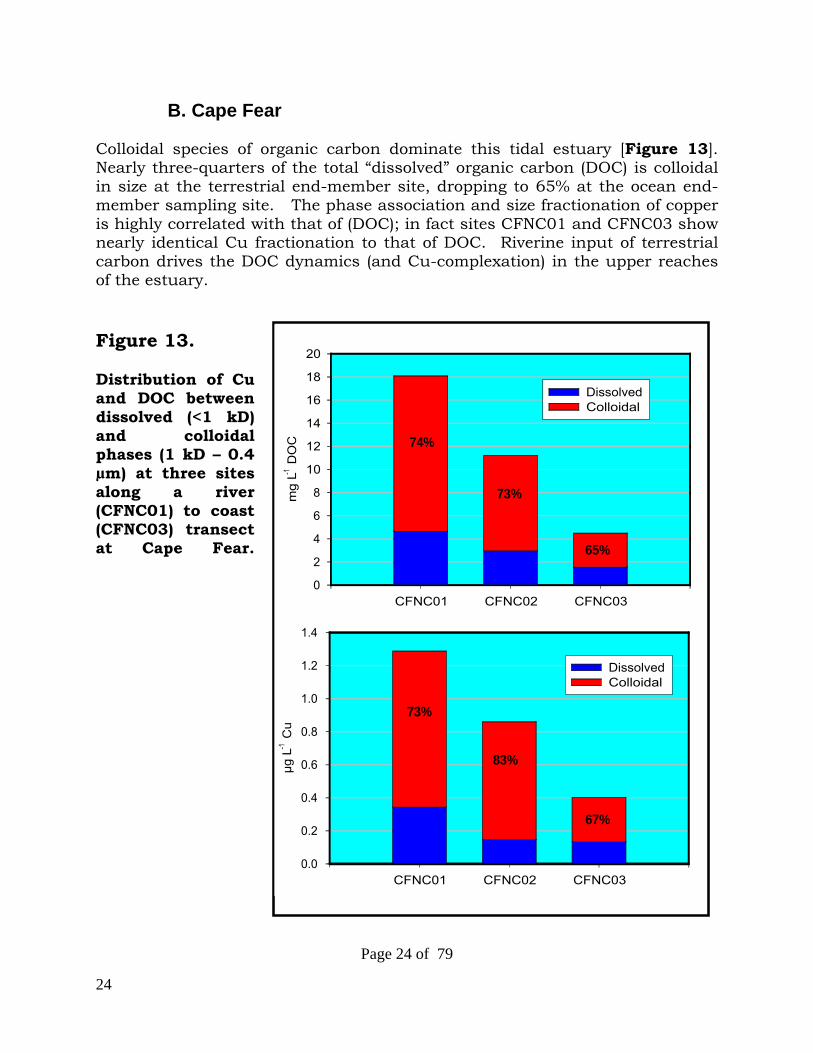
B. Cape Fear

Colloidal species of organic carbon dominate this tidal estuary [Figure 13]. Nearly three-quarters of the total “dissolved” organic carbon (DOC) is colloidal in size at the terrestrial end-member site, dropping to 65% at the ocean end-member sampling site. The phase association and size fractionation of copper is highly correlated with that of (DOC); in fact sites CFNC01 and CFNC03 show nearly identical Cu fractionation to that of DOC. Riverine input of terrestrial carbon drives the DOC dynamics (and Cu-complexation) in the upper reaches of the estuary. Figure 13. Distribution of Cu and DOC between dissolved (<1 kD) and colloidal phases (1 kD – 0.4 µm) at three sites along a river (CFNC01) to coast (CFNC03) transect at Cape Fear.

25

Page 25 of 79

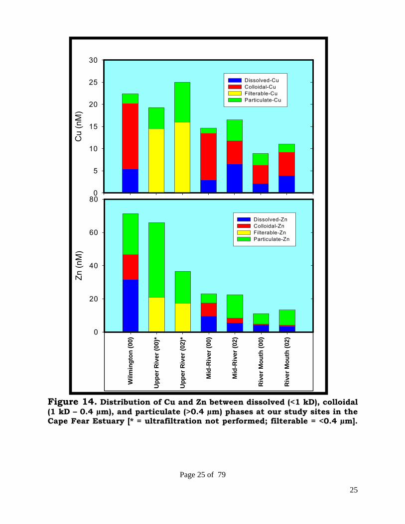
Figure 14. Distribution of Cu and Zn between dissolved (<1 kD), colloidal (1 kD – 0.4 µm), and particulate (>0.4 µm) phases at our study sites in the Cape Fear Estuary [* = ultrafiltration not performed; filterable = <0.4 µm].

Cu

(nM

)

0

5

10

15

20

25

30

Dissolved-Cu Colloidal-Cu Filterable-Cu Particulate-Cu

Wilm

ingt

on (0

0)

Upp

er R

iver

(00)

*

Upp

er R

iver

(02)

*

Mid

-Riv

er (0

0)

Mid

-Riv

er (0

2)

Riv

er M

outh

(00)

Riv

er M

outh

(02)

Zn (n

M)

0

20

40

60

80

Dissolved-Zn Colloidal-Zn Filterable-Zn Particulate-Zn

26

Page 26 of 79

A very high degree of consistency is observed in metal levels and phase partitioning at a given site [Figure 14]. Concentrations of both metals drop significantly as one moves downstream from Wilmington to the mouth of the Cape Fear River. This decline is greater for Zn (70 nM to 15 nM) than for Cu (24 nM to 10 nM). While colloidal forms of Cu are the dominant phase, colloidal species of Zn are much less important, with only minor contributions at the river mouth. In contrast, particulate forms of Zn are the dominant phase, with particulate forms of Cu contributing, but much less so. The dissolved (<1 kDa) fraction of Cu is typically less than 30% of total metal at all sites. Trace metal and DOC Levels in Cape Fear can be modeled with a two end-member mixing model (Cape Fear River & Coastal Seawater) [Figure 15]. DOC and metal in <1 kDa phases exhibit only minor non-conservative behavior. Figure 15. Two end-member mixing model for Cape Fear.

Cu-complexing ligand at Cape Fear [Figure 16] is found to be predominantly associated with colloidal sized phases at both upper and mid-estuary sites. An input of <1 kD sized ligand in the ocean end-member site results in a nearly 50:50 distribution between colloidal and dissolved phases.

salinity0 5 10 15 20 25 30 35

DO

C-0

.4µm

(µM

)

200

400

600

800

1000

1200

1400

1600

Cu-

0.4µ

m (n

M)

4

6

8

10

12

14

16

18

20

22

Cu-

1kD

(nM

)

1

2

3

4

5

6

DO

C-1

kD (µ

M)

100

150

200

250

300

350

400

450

DOC - 0.4 µmCu - 0.4 µmCu - 1 kDDOC - 1 kD

27

Page 27 of 79

Figure 16. Phase distribution of Cu-complexing ligand at three sites at Cape Fear.

CFNC03

Dissolved = 8% Colloidal = 92%

CFNC02

Dissolved = 40%Colloidal = 60%

CFNC01


Total Cu Ligand = 113 nM

Total Cu Ligand = 68.3 nM


28

Page 28 of 79

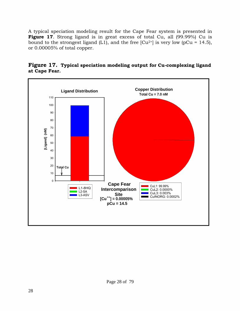
A typical speciation modeling result for the Cape Fear system is presented in Figure 17. Strong ligand is in great excess of total Cu, all (99.99%) Cu is bound to the strongest ligand (L1), and the free [Cu2+] is very low (pCu = 14.5), or 0.00005% of total copper. Figure 17. Typical speciation modeling output for Cu-complexing ligand at Cape Fear.

Ligand Distribution

[Lig

and]

(nM

)

0

10

20

30

40

50

60

70

80

90

100

110

Total Cu

L1-8HQ L2-SAL3-ASV

Copper DistributionTotal Cu = 7.0 nM

CuL1: 99.99%CuL2: 0.0000% CuL3: 0.003% CuINORG: 0.0002%

Cape FearIntercomparison

Site[Cu++] = 0.00005%

pCu = 14.5

29

Page 29 of 79

C. Norfolk – Hampton Roads The Norfolk system is more complex both hydrographically and geochemically than the Cape Fear system, however, colloidal phases remain critically important [Figure 18]. Several geochemically contrasting riverine sources of Cu-complexing ligand are evident, including the James River (with a large proportion of < 1 kD DOC and Cu) and the Elizabeth River (with a higher proportion of colloidal DOC and Cu). As in the Cape Fear system, colloidal Cu levels are strongly related to colloidal carbon levels; however, carbon levels are significantly lower, and the nature of carbon more variable, so the relationship is not as tight. Site NRF-A shows evidence of coagulation/aggregation of DOC and Cu-ligand associated with aggregate precursors. Figure 18. Distribution of Cu and DOC between dissolved (<1 kD) and colloidal phases (1 kD – 0.4 µm) at selected focus sites at Norfolk.

NRF-1 NRF-C NRF-A NRF-B

mg

L-1 D

OC

0.00.51.01.52.02.53.03.54.04.55.05.56.0

DissolvedColloidal

NRF-1 NRF-C NRF-A NRF-B

µg L

-1 C

u

0.00.20.40.60.81.01.21.41.61.82.02.22.42.6

DissolvedColloidal

57% 44%

33%

58% 41%

57%27%

16%

30

Page 30 of 79

Figure 19. Distribution of Cu and Zn between dissolved (<1 kD), colloidal (1 kD – 0.4 µm), and particulate (>0.4 µm) phases at our study sites in the Norfolk Estuary [* = ultrafiltration not performed; filterable = <0.4 µm].

Cu

(nM

)

0

10

20

30

40

50

60

70

80

90


Ham

pton

Rds

(00)

*H

ampt

on R

ds (0

1)H

ampt

on R

ds (0

2)H

ampt

on R

ds (0

3)*

N. G

rane

y Is

le (0

1)N

. Gra

ney

Isle

(02)

*N

. Gra

ney

Isle

(03)

*Ja

mes

Riv

er (0

1)*

Jam

es R

iver

(02)

Jam

es R

iver

(03)

*N

anse

mon

d R

. (00

)*N

anse

mon

d R

. (01

)*S

. Gra

ney

Isle

(00)

*D

egau

ssin

g S

ite (0

0)U

pper

Eliz

abet

h (0

0)*

Upp

er E

lizab

eth

(01)

Upp

er E

lizab

eth

(02)

Upp

er E

lizab

eth

(03)

*Lo

wer

Eliz

abet

h (0

1)Lo

wer

Eliz

abet

h (0

2)Lo

wer

Eliz

abet

h (0

3)*

Sou

th E

lizab

eth

(03)

*

Zn (n

M)

0

50

100

150

200

250

350400

Dissolved-Zn Colloidal-Zn Filterable-Zn Particulate-Zn

31

Page 31 of 79

A very high degree of consistency is observed in metal levels and phase partitioning at most sites [Figure 19] (e.g. compare four years of sampling at Hampton Rds, and four years of sampling at the Upper Elizabeth sites). Concentrations of both metals at the ocean end-member site (Hampton Rds) are comparable to those observed at the ocean end-member site at Cape Fear, however, river and harbor concentrations of metals are significantly greater in the Norfolk system than at Cape Fear (40-80 nM versus 20-25 nM Cu and 150-400 nM versus 60-70 nM Zn. Colloidal forms of Cu are a co-dominant phase at most sites, however, colloidal species of Zn are much less important, with only minor contributions at all sites studied. In contrast, particulate forms of Zn are the dominant phase at all sites impacted by the James River, including the ocean end-member. Particulate forms of Zn at the Elizabeth River sites are significant but not dominant. Significant (20-40%) particulate contribution to total Cu levels is also observed. Dissolved (< 1 kD) Cu levels are typically less than 50% of total Cu levels at all study sites, and a similar dissolved fraction is measured at James River impacted sites for Zn. However in the Elizabeth River system dissolved fractions of Zn are much greater (>80%). Colloidal sized (1 kD – 0.4 µm) Cu-binding ligands typically represent 50-60% of total ligand in the Norfolk system (Figure 20). Very high levels of ligand are measured at site NRF-C, the Elizabeth river end-member (this river drains a large wetland and in doing so acquires high levels of DOC). Figure 20. Phase distribution of Cu-complexing ligand at two sites in the Norfolk system.

NRF-A

Dissolved = 44%

Colloidal = 56%

NRF-C



Total Cu Ligand = 196 nM

32

Page 32 of 79

A typical speciation modeling result for a Norfolk site with relatively high levels of both total Cu and DOC is presented in Figure 21. The general copper speciation pattern is intermediate between that determined at Cape Fear and that in San Diego Bay. Total Cu levels are approaching strong (L1) ligand concentrations, and therefore a small fraction of Cu is bound to weaker L2 ligands. However, little or no Cu is associated with ASV ligands. Free Cu2+ is still very small however (pCu = 13.2), though an order of magnitude higher than at Cape Fear when expressed as a percentage of total Cu. Modeling predicts a 54%/46% distribution between colloidal and dissolved phases, nearly identical to the ratio actually measured by ultrafiltration, lending strong support to that approach. Figure 21. Typical speciation modeling output for Cu-complexing ligand at Norfolk.

Ligand distribution

[Lig

and]

(nM

)

0

50

100

150

200

Copper distribution

total Cu = 34.6 nM[Cu2+] = 0.0005%

pCu = 13.2

Colloidal (1 kDa - 0.4µm)Dissolved (<1 kDa)

L3 (ASV)L2 (CSV - SA)L1 (CSV - 8HQ)

TotalCu

Copper and Cu-binding ligand distribution - NRF-CNorfolk, July 2001

46% dissolved

54% colloidal

33

Page 33 of 79

D. San Diego Bay At the other end of the gradient from high DOC fluvial/terrestrial dominated systems to low DOC/authothonous dominated systems is San Diego Bay. Fluvial inputs are minimal and DOC levels are nearly an order-of-magnitude lower. DOC and ligand levels are regulated by a balance between production of authothonous carbon and loss through sedimentation/coagulation and hydrologic flushing. Colloidal carbon fractions increase from 20-25% at Bay mouth to 40-50% in South Bay, a trend consistent with increasing water residence time (Figure 22). Colloidal Cu levels are high (40-55%) and are not simply related to bulk colloidal carbon, suggesting the presence of a very strong ligand, but at low concentrations. The observed trends in colloidal Cu fraction also reflect the parallel increases of ligand and total Cu as one moves from Bay mouth to South Bay. Figure 22. Distribution of Cu and DOC between dissolved (<1 kD) and colloidal phases (1 kD – 0.4 µm) along a transect from South Bay (SDFO4) to Bay Mouth (SDFO1) in San Diego Bay.

SDF04 SDF05 SD09FB SDF03 SDF02 SD09FC SDF01

mg

L-1 D

OC

0.0

0.2

0.4

0.6

0.8

1.0

1.2

1.4

1.6

1.8

2.0

2.2

DissolvedColloidal

SDF04 SDF05 SD09FB SDF03 SDF02 SD09FC SDF01

µg L

-1 C

u

0.0

0.5

1.0

1.5

2.0

2.5

3.0

3.5

DissolvedColloidal

39% 48%

48%

43%

46%

35%28%

47%

37% 18%27%

54%

51%

36%

34

Page 34 of 79

Figure 23. Distribution of Cu and Zn between dissolved (<1 kD), colloidal (1 kD – 0.4 µm), and particulate (>0.4 µm) phases at our study sites in San Diego Bay [* = ultrafiltration not performed; filterable = <0.4 µm].

Cu

(nM

)

0

10

20

30

40

50

60

70120140


Bay

Mou

th (0

101)

Bay

Mou

th (0

501)

Bay

Mou

th (0

901)

Bay

Mou

th (0

202)

Bay

Mou

th (0

502)

SPA

WR

(010

1)Sh

elte

r Is.

(010

1)Sh

elte

r Is.

(090

1)Sh

elte

r Is.

(020

2)H

arbo

r Is.

(010

1)H

arbo

r Is.

(050

1)H

arbo

r Is.

(090

1)H

arbo

r Is.

(020

2)H

arbo

r Is.

(050

2)Lo

wer

N. B

ay (0

101)

Upp

er S

. Bay

(010

1)U

pper

S. B

ay (0

501)

Upp

er S

. Bay

(090

1)U

pper

S. B

ay (0

202)

Mid

S. B

ay (0

101)

Mid

S. B

ay (0

501)

Mid

S. B

ay (0

901)

Mid

S. B

ay (0

202)

Mid

S. B

ay (0

502)

Far S

. Bay

(010

1)Fa

r S. B

ay (0

501)

Far S

. Bay

(020

2)Fa

r S. B

ay (0

502)

Zn (n

M)

0

50

100

150

200

250 Dissolved-Zn Colloidal-Zn Filterable-Zn Particulate-Zn

35

Page 35 of 79

As observed in our two other study systems, metal levels and phase partitioning at most sites are quite consistent on a seasonal and annual basis [Figure 23] (e.g. compare four samples each at Far S. Bay, Mid S. Bay, and Harbor Is. sites – (the 0501 data are an exception however)). Concentrations of Cu at the ocean end-member site (Bay Mouth) are more variable (ranging from 5 – 20 nM) and typically lower than at Norfolk and Cape Fear. This reflects both the large contrast and sharp gradient in metal concentrations between harbor and ocean and varying tidal mixing conditions. Zinc concentrations, like those of Cu, are also variable at the ocean end-member site; however levels are comparable to those measured at Norfolk and Cape Fear. Copper and Zn concentrations in San Diego Bay proper are similar to those measured in the Norfolk system (40-60 nM Cu; 150-200 nM Zn), but again significantly higher than at Cape Fear (20-25 nM Cu and 60-70 nM Zn. Colloidal forms of Cu are a co-dominant phase at most sites, however, colloidal species of Zn are much less important, with only minor contributions at all sites studied. Unlike in the two other study systems, particulate forms of Zn are only a relatively minor component of the total metal. The one exception to this “rule” are samples collected in May of 2001, where very large particulate fractions of Zn (and Cu) were measured – coinciding with a major algal bloom in the Bay. Particulate contributions to total Cu levels were more significant (15-30%) than that measured for Zn. Dissolved (< 1 kD) Cu levels are typically less than 40% of total Cu levels at all study sites, however dissolved fractions of Zn are typically much greater (>85%). Except for the ocean end-member site (where < 1 kD Cu-binding ligands dominate), colloidal phases completely dominate the Cu-binding ligand size distribution (Figure 24). Between 70 and 80% of total strong-ligand binding capacity in San Diego Bay proper is associated with colloidal species. This is in contrast to most sites in the other study systems, where strong-ligand binding capacity more closely tracked DOC levels. Note that strong ligand levels double from the Bay Mouth (18 nM) to North Bay (36 nM), and double again from North Bay to South Bay (73 nM)

36

Page 36 of 79

Figure 24. Phase distribution of Cu-complexing ligand at five sites in San Diego Bay, representing a transect from Bay Mouth (SDF01) to South Bay (SDF04).

SDF03


SDF02


SDF01





SDF05



SDF04



37

Page 37 of 79

A typical speciation modeling result for San Diego Bay Mouth Site is presented in Figure 25. Total Cu levels are similar to those at Cape Fear, however the ligand levels are much lower, and therefore, the strongest ligands are saturated. Some Cu is bound to weaker ligands (L2), a small fraction even to very weak (ASV) ligands. Free [Cu2+] is much higher than at Cape Fear (pCu = 12.5). Figure 25. Typical speciation modeling output for Cu-complexing ligand in San Diego Bay – Bay Mouth.

Ligand Distribution

[Lig

and]

(nM

)

0

10

20

30

40

50

60

70

Total Cu

L1-8HQ L2-SAL3-ASV


CuL1: 57.4%CuL2: 41.8%CuL3: 0.6% CuINORG: 0.2%

San Diego BaySite 3

[Cu++] = 0.0036%pCu = 12.5

38

Page 38 of 79

A typical speciation modeling result for San Diego Bay – South Bay Site is presented in Figure 26. Levels of strong ligand and Cu are both greater than at the Bay mouth. A large majority of the Cu is bound to the strongest ligands (likely algal-sourced), and much less is bound to weaker ligands than at the Bay mouth. Figure 26. Typical speciation modeling output for Cu-complexing ligand in San Diego Bay – South Bay.

Ligand Distribution

[Lig

and]

(nM

)

0

10

20

30

40

50

60

70

80

90

100

110

120

Total Cu

L1-8HQ L2-SAL3-ASV


CuL1: 87.6%CuL2: 12.3%CuL3: 0.04%CuINORG: 0.06%

San Diego BaySite 27

[Cu++] = 0.0007%pCu = 12.6

39

Page 39 of 79

E. Filterable Copper – Strong Ligand Comparison Total levels of strong copper-binding ligand are in large excess of Cu levels in both the Cape Fear and Norfolk systems (Figure 27). At Cape Fear, strong ligand levels range from 80 to over 270 nM (modal value of ~100 nM) and filterable Cu concentrations are < 20 nM. At Norfolk, strong ligand levels range from 60 to nearly 400 nM, with filterable Cu concentrations in the range of 20-50 nM. However in San Diego, concentrations of ligand and copper are similar, and many instances, Cu levels exceed strong ligand (Figure 27). Bioavailability of Cu is predicted to be significantly greater under the conditions measured in San Diego in comparison to other study systems. Figure 27. Strong copper ligand concentrations compared with filterable copper levels at Cape Fear, San Diego Bay, and Norfolk.

Strong Cu Ligand LevelsCompared With

Filterable Cu Levels

CFN

C01

CF0

402C

CFN

C02

CF0

402B

CFN

C03

CF0

402A

SDF0

4SD

0501

CSD

0202

CSD

0502

CSD

F05

SD09

01B

SD02

02B

SD05

02D

SDF0

3SD

0501

BSD

F02

SD09

01C

SD02

02D

SD05

02B

SDF0

1SD

0501

ASD

0901

ASD

0202

ASD

0502

E

NR

F100

2DN

RF0

603D

NR

F070

1CN

RF1

002C

NR

F060

3CN

RF1

002E

NR

F070

1AN

RF0

603A

[Cu-

Liga

nd] a

nd [C

u f] (n

M)

0

20

40

60

80

100

120

140

160

180

200

220

240

Total Ligand Filterable Cu

Cape Fear

San Diego

Norfolk

274 384

40

Page 40 of 79

F. Chelex Lability Summary

Uptake of copper and zinc onto a chelating resin (Chelex-100) was used as a measure of the lability of metal in the aqueous samples. Fundamentally this is a metric of the dissociation kinetics (lability) of metal-ligand associations and therefore complements the voltammetry studies which are equilibrium based. It must be stressed that kinetic lability is not necessarily correlated with the stability constant (equilibrium-derived) – it’s possible for a very strong metal-ligand association to exhibit fast dissociation kinetics. We specially prepared Chelex columns and operated them under conditions that would be expected to retain only the free and very labile metal ion. This work is detailed in our publication: Shafer, M., S. Hoffmann, J. Overdier, and D. Armstrong. 2004. Physical and kinetic speciation of Copper and Zinc in three geochemically contrasting marine estuaries. Environmental Science and Technology 38(14):3810-3819., and only a brief mention of this sizable effort is presented here. Figure 28. Chelex non-labile Cu versus colloidal Cu in the 3 systems.

Colloidal versus

Chelex Non-Labile Copper

Colloidal Copper (nM)0 5 10 15 20 25 30

Che

lex

Non

-Lab

ile C

oppe

r (nM

)

0

10

20

30

40

50

San Diego: r2=0.89Cape Fear: r2=0.91Norfolk: r2=0.88

41

Page 41 of 79

A very strong relationship exists between Chelex non-labile Cu (i.e. the Cu not retained on the columns) and colloidal copper (Figure 28), indicating that Cu associated with colloids is likely not labile and therefore less bioavailable. The lines defining the relationships for San Diego and Cape Fear pass through the origin, suggesting that all non-labile copper is represented by colloidal phases. However, at Norfolk, a significant y-intercept is measured (~10 nM – Figure 28) signifying the presence of non-labile Cu species in the < 1 kD dissolved fraction. The presence of strong synthetic ligands such as EDTA or NTA, sourced from waste water treatment plant discharges, in the Norfolk samples, could explain this finding. A comparison of the measured physical and kinetic speciation of Cu and Zn at Bay Mouth sites at Cape Fear and San Diego is presented in Figure 29. Filterable (dissolved + colloidal) Cu levels are 50% higher (10 versus 6.5 nM) at San Diego; however, the colloidal fraction is significantly greater at Cape Fear. The labile/non-labile distribution of Cu mirrors that of the dissolved-colloidal fractionation. Figure 29. Comparison of physical and kinetic speciation of Cu and Zn at Bay Mouth Sites at Cape Fear and San Diego.

nM C

u or

Zn

0

2

4

6

8

10

12

Dissolved Colloidal Labile NonLabile

Cape Fear San Diego

Copper

Copper

ZincZinc

42

Page 42 of 79

Filterable Zn concentrations are comparable in the two systems, as is the distribution between dissolved and colloidal phases – both systems exhibiting a much greater Zn dissolved fraction than that for Cu. The greater dissolved fraction for Zn is mirrored in the Zn lability data, with lability fractions approaching 90% in San Diego. Though labile Zn fractions at Cape Fear are significantly greater than those for Cu, a substantial non-labile fraction is still measurable. VII. Ligand & Dissolved Organic Matter Character (DOM) Significant differences in the “quality” of the organic matter are apparent, as shown by contrasts in carbon normalized Cu-binding ligand levels (Figure 30) and Specific UV-Absorbance - SUVA-254 nm (Figure 31). Normalized dissolved strong ligand levels in San Diego range over a factor of 2 (from 110-210 µM/M). In Norfolk, the overall dissolved levels are higher, but a factor of 2 range in normalized ligand abundance is also observed [from 200-400 µM/M]. A much larger range is measured in the Cape Fear system (60-450 µM/M) resulting primarily from dilution of strong ligand by very high DOC at the river end-member sites. Colloidal phases in all three systems, particularly at sites with high algal production, are dramatically enriched in Cu-binding ligand in comparison with dissolved phases. This colloidal enrichment is most evident in San Diego Bay, the system with the greatest autochthonous carbon production. It’s clear from these normalized data, and very important to mention, that the strong Cu-binding ligand at all sites and systems represents only a very small fraction of the DOM (irregardless of specific binding site stoiciommetry). At typical values of 100-200 µM/M strong ligand abundance corresponds to only 100-200 PPM in the carbon. Even in the highly enriched colloidal fractions strong ligand abundance rarely exceeds 1000 PPM (0.1%). SUVA-254 data demonstrate the predominantly terrestrial character of the DOM in the Norfolk and Cape Fear systems (higher SUVA values are indicators of increasing aromatic content of the DOC). At Cape Fear, the ultrafiltration retentates (higher molecular weight fractions) have a greater aromatic content compared to the permeates (1 and 10 kDa). However in San Diego, the opposite is true, again indicating a remarkably different pool of DOM than that found in the Cape Fear system. SUVA values increase from Bay Mouth to South Bay in San Diego, likely reflecting the longer hydraulic residence time and more extensive DOM processing in South Bay.

43

Page 43 of 79

Figure 30. Comparison of organic carbon normalized strong Cu ligand levels between dissolved (1 kDa permeate) and colloidal (1 kDa retentate) molecular weight fractions in our three study systems.

Strong Cu Ligand Levels Normalized to Organic CarbonComparison between Sites and Size Fraction

CFN

C01

CFN

C02

CF0

402B

CFN

C03

CF0

402A

NR

F100

2CN

RF0

701C

NR

F100

2DN

RF0

701A

SD02

02C

SDF0

4SD

0202

BSD

F05

SDF0

3SD

0202

DSD

F02

SD02

02A

SDF0

1

[Stro

ng L

igan

d] /

[Car

bon]

(µM

/M)

0

100

200

300

400

500

600

700

800

900

1000

DissolvedColloidalCape Fear Norfolk San Diego

1890 1440

44

Page 44 of 79

Figure 31. Comparison of Specific UV Absorbance (SUVA- 254 nm) between small (1 kDa permeate) and large (1 kDa retentate) molecular weight fractions in our three study systems.

Norfolk

Hampton Roads James River ShipYards Elizabeth River

SU

VA

(L/c

m)

0

100

200

300

400

5001 kD Retentate 1 kD Permeate

CapeFear

River Mouth Mid-River

SU

VA

(L/c

m)

0

100

200

300

400

500 1kD Retentate 10kD Retentate 10kD Permeate 1kD Permeate

San Diego

Bay Mouth Harbor Island S. Crndo. Bridge South Bay

SU

VA

(L/c

m)

0

100

200

300

400

5001kD Retentate 1kD Permeate

45

Page 45 of 79

Algal pigment levels show a strong correlation with Cu-binding ligand concentrations (Figure 32), suggesting that strong ligands are derived from algal exudates. In San Diego the data (slopes) suggests that strong ligand is solely derived from algal production, whereas on the East Coast a baseline contribution from non-algal sources is also indicated. Figure 32. Strong Cu-binding ligand concentration – relationship to algal pigments (Fucoxanthin – a diatom accessory pigment) at study sites.

.

Metal-Binding Ligandas a function of

Diatom Photo-Pigment

Fucoxanthin (ng L-1 )0 500 1000 1500 2000 2500 3000 3500 4000

Stro

ng C

u-bi

ndin

g Li

gand

(nM

)

0

50

100

150

200

250

West Coast (San Diego)East Coast (Norfolk+Cape Fear)

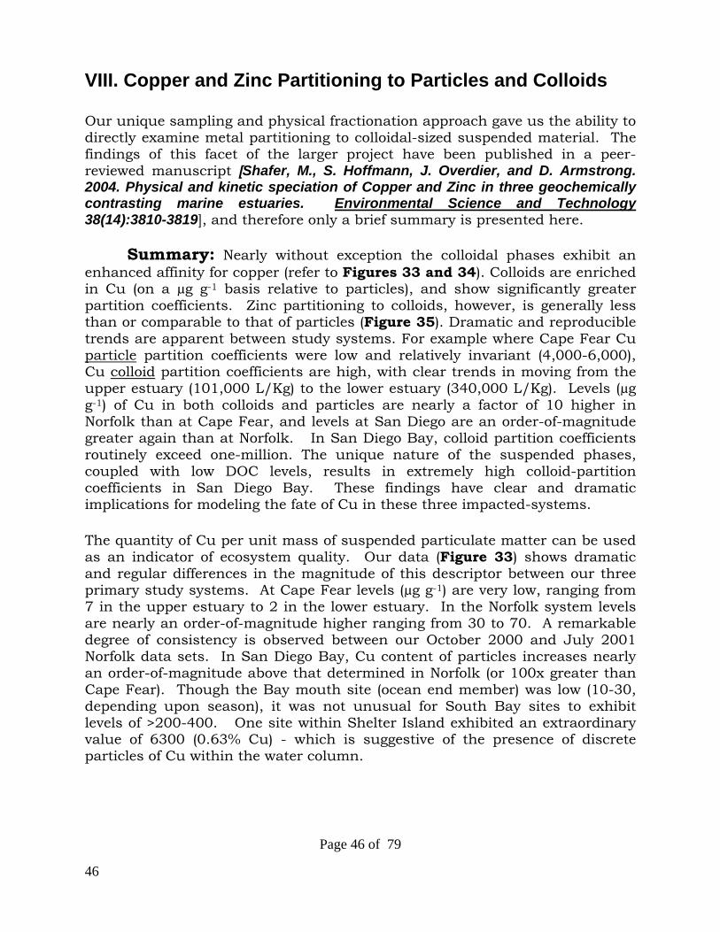
46

Page 46 of 79

VIII. Copper and Zinc Partitioning to Particles and Colloids Our unique sampling and physical fractionation approach gave us the ability to directly examine metal partitioning to colloidal-sized suspended material. The findings of this facet of the larger project have been published in a peer-reviewed manuscript [Shafer, M., S. Hoffmann, J. Overdier, and D. Armstrong. 2004. Physical and kinetic speciation of Copper and Zinc in three geochemically contrasting marine estuaries. Environmental Science and Technology 38(14):3810-3819], and therefore only a brief summary is presented here.

Summary: Nearly without exception the colloidal phases exhibit an enhanced affinity for copper (refer to Figures 33 and 34). Colloids are enriched in Cu (on a µg g-1 basis relative to particles), and show significantly greater partition coefficients. Zinc partitioning to colloids, however, is generally less than or comparable to that of particles (Figure 35). Dramatic and reproducible trends are apparent between study systems. For example where Cape Fear Cu particle partition coefficients were low and relatively invariant (4,000-6,000), Cu colloid partition coefficients are high, with clear trends in moving from the upper estuary (101,000 L/Kg) to the lower estuary (340,000 L/Kg). Levels (µg g-1) of Cu in both colloids and particles are nearly a factor of 10 higher in Norfolk than at Cape Fear, and levels at San Diego are an order-of-magnitude greater again than at Norfolk. In San Diego Bay, colloid partition coefficients routinely exceed one-million. The unique nature of the suspended phases, coupled with low DOC levels, results in extremely high colloid-partition coefficients in San Diego Bay. These findings have clear and dramatic implications for modeling the fate of Cu in these three impacted-systems. The quantity of Cu per unit mass of suspended particulate matter can be used as an indicator of ecosystem quality. Our data (Figure 33) shows dramatic and regular differences in the magnitude of this descriptor between our three primary study systems. At Cape Fear levels (µg g-1) are very low, ranging from 7 in the upper estuary to 2 in the lower estuary. In the Norfolk system levels are nearly an order-of-magnitude higher ranging from 30 to 70. A remarkable degree of consistency is observed between our October 2000 and July 2001 Norfolk data sets. In San Diego Bay, Cu content of particles increases nearly an order-of-magnitude above that determined in Norfolk (or 100x greater than Cape Fear). Though the Bay mouth site (ocean end member) was low (10-30, depending upon season), it was not unusual for South Bay sites to exhibit levels of >200-400. One site within Shelter Island exhibited an extraordinary value of 6300 (0.63% Cu) - which is suggestive of the presence of discrete particles of Cu within the water column.

47

Page 47 of 79

Copper Content of Particles & Colloids

CF-Wilm

ington

CF-mid River

CF-River Mouth

NF-Hampton Roads

NF-Graney Island

NF-Upper Elizabeth

NF-Lower Elizabeth

SD-Bay Mouth (01)

SD-Bay Mouth (09)

SD-Harbor Island (01)

SD-Harbor Island (09)

SD-Crndo. Bridge (01)

SD-mid South Bay (01)

SD-mid South Bay (09)

SD-South Bay (01)

ug/g

Cu

0

200

400

600

800

1000

1200

1400

1600

1800

2000

2200

2400

ugg-Particles ugg-Colloids

Figure 33. Copper content of particles and colloids in the three study systems.

48

Page 48 of 79

Figure 34. Copper: Particle and colloid Partition Coefficient.

CF-Wilm

ington

(00)

CF-mid

River (

00)

CF-mid

River (

02)

CF-Rive

r Mou

th (00

)

CF-Rive

r Mou

th (02

)

NF-Ham

pton R

oads

(01)

NF-Ham

pton R

oads

(02)

NF-Gran

ey Is

land (

01)

NF-Gran

ey Is

land (

02)

NF-James

Rive

r (02

)

NF-Upp

er Eliz

abeth

(01)

NF-Upp

er Eliz

abeth

(02)

NF-Lower

Elizabe

th (01

)

NF-Lower

Elizabe

th (02

)

SD-Bay

Mou

th (01

)

SD-Bay

Mou

th (09

)

SD-Bay

Mou

th (02

)

SD-Harb

or Isl

and (

01)

SD-Harb

or Isl

and (

09)

SD-Harb

or Isl

and (

02)

SD-Crnd

o. Brid

ge (0

1)

SD-mid

South

Bay (0

1)

SD-mid

South

Bay (0

9)

SD-mid

South

Bay (0

2)

SD-Sou

th Bay

(01)

SD-Sou

th B

ay (0

2)

KD (

L/K

g)

0.0

2.0e+5

4.0e+5

6.0e+5

8.0e+5

1.0e+6

1.2e+6

1.4e+6

2.5e+6

Kd-Particles Kd-Colloids

CopperParticle & Colloid

Partition Coefficient

49

Page 49 of 79

Figure 35. Zinc: Particle and colloid Partition Coefficient.

CF-Wilm

ington

(00)

CF-mid

River (

00)

CF-mid

River (

02)

CF-Rive

r Mou

th (00

)

CF-Rive

r Mou

th (02

)

NF-Ham

pton R

oads

(01)

NF-Ham

pton R

oads

(02)

NF-Gran

ey Is

land (

00)

NF-Gran

ey Is

land (

01)

NF-James

Rive

r (02

)

NF-Upp

er Eliza

beth

(01)

NF-Upp

er Eliza

beth

(02)

NF-Lower

Elizabe

th (01

)

NF-Lower

Elizabe

th (02

)

SD-Bay

Mou

th (01

)

SD-Bay

Mou

th (09

)

SD-Bay

Mou

th (02

)

SD-Harb

or Isl

and (

01)

SD-Harb

or Isl

and (

09)

SD-Harb

or Isl

and (

02)

SD-Crnd

o. Brid

ge (0

1)

SD-mid

South

Bay (0

1)

SD-mid

South

Bay (0

9)

SD-mid

South

Bay (0

2)

SD-Sou

th Bay

(01)

SD-Sou

th B

ay (0

2)

KD (

L/K

g)

0.0

1.0e+5

2.0e+5

3.0e+5

4.0e+5

5.0e+5

6.0e+5

Kd-Particles Kd-Colloids

ZincParticle & Colloid

Partition Coefficient

50

Page 50 of 79

Particle-partition coefficients, though not strictly thermodynamic constants, are frequently used to express the net “affinity” of a particle for a metal. We have determined these Kd values for all our sites and not unexpectedly the trends observed follow those determined for the micrograms per gram descriptor (above). Cape Fear Kd’s are very low (4,000-6,000 L/Kg), reflecting both low Cu levels on particles and competition from high DOC levels. Norfolk Kd levels are typically in the range of 20,000 to 40,000, a magnitude not atypical for many moderately-impacted systems. However, in San Diego Bay Kds were nearly always greater than 50,000, with several sites in the hundreds of thousands. It’s apparent that the nature of the suspended particles in San Diego Bay coupled with low DOC levels, result in a strong preference of Cu for particulate phases. Cu Kd-colloid is strongly predicted in all three study systems from DOC levels (Figure 36). The corresponding DOM-Cu Kd-particle relationship is significant but not as strong as the colloid relationship. Figure 36. Relationships between DOC and Colloid and Particle Partition Coefficients for Copper.

Copper Kd versus DOC

DOC (µM)100 1000

Kd (

L/K

g)

1e+4

1e+5

1e+6

Particle Colloid

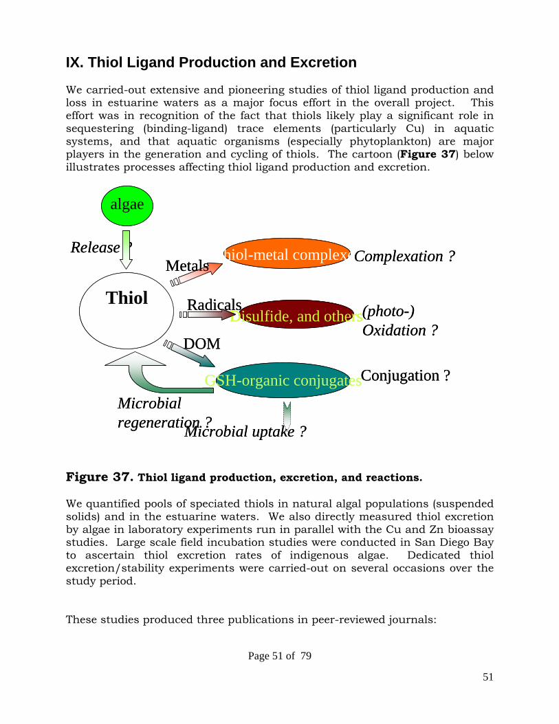
51

Page 51 of 79

IX. Thiol Ligand Production and Excretion We carried-out extensive and pioneering studies of thiol ligand production and loss in estuarine waters as a major focus effort in the overall project. This effort was in recognition of the fact that thiols likely play a significant role in sequestering (binding-ligand) trace elements (particularly Cu) in aquatic systems, and that aquatic organisms (especially phytoplankton) are major players in the generation and cycling of thiols. The cartoon (Figure 37) below illustrates processes affecting thiol ligand production and excretion.

Release ?

algae

ThiolDisulfide, and others(photo-)

Oxidation ?

Thiol-metal complexes

GSH-organic conjugates

Metals Complexation ?

Radicals

DOM

Conjugation ?

Microbial uptake ?

Microbial regeneration ?

Release ?

algae

ThiolDisulfide, and others(photo-)

Oxidation ?

Thiol-metal complexes

GSH-organic conjugates

Metals Complexation ?

Radicals

DOM

Conjugation ?

Microbial uptake ?

Microbial regeneration ?

Figure 37. Thiol ligand production, excretion, and reactions. We quantified pools of speciated thiols in natural algal populations (suspended solids) and in the estuarine waters. We also directly measured thiol excretion by algae in laboratory experiments run in parallel with the Cu and Zn bioassay studies. Large scale field incubation studies were conducted in San Diego Bay to ascertain thiol excretion rates of indigenous algae. Dedicated thiol excretion/stability experiments were carried-out on several occasions over the study period. These studies produced three publications in peer-reviewed journals:

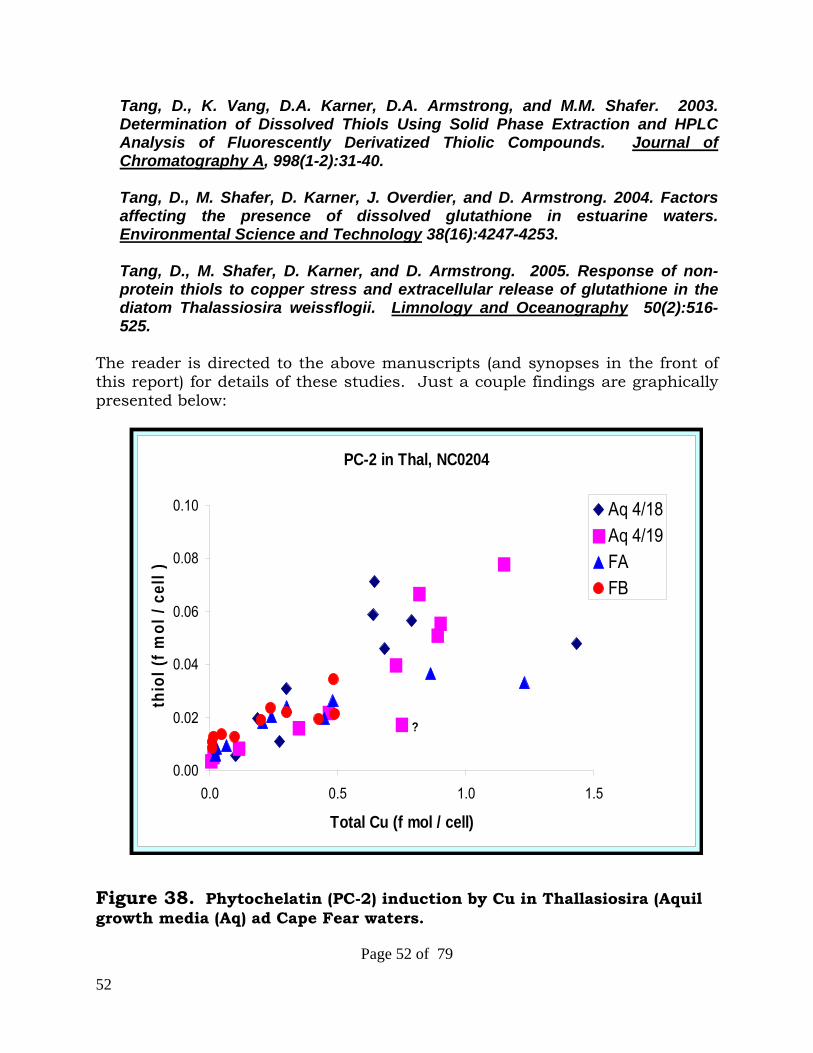
52

Page 52 of 79

Tang, D., K. Vang, D.A. Karner, D.A. Armstrong, and M.M. Shafer. 2003. Determination of Dissolved Thiols Using Solid Phase Extraction and HPLC Analysis of Fluorescently Derivatized Thiolic Compounds. Journal of Chromatography A, 998(1-2):31-40. Tang, D., M. Shafer, D. Karner, J. Overdier, and D. Armstrong. 2004. Factors affecting the presence of dissolved glutathione in estuarine waters. Environmental Science and Technology 38(16):4247-4253. Tang, D., M. Shafer, D. Karner, and D. Armstrong. 2005. Response of non-protein thiols to copper stress and extracellular release of glutathione in the diatom Thalassiosira weissflogii. Limnology and Oceanography 50(2):516-525.

The reader is directed to the above manuscripts (and synopses in the front of this report) for details of these studies. Just a couple findings are graphically presented below: Figure 38. Phytochelatin (PC-2) induction by Cu in Thallasiosira (Aquil growth media (Aq) ad Cape Fear waters.

PC-2 in Thal, NC0204

0.00

0.02

0.04

0.06

0.08

0.10

0.0 0.5 1.0 1.5

Total Cu (f mol / cell)

thio

l (f m

ol /

cell

)

Aq 4/18Aq 4/19FAFB

?

53

Page 53 of 79

A strong linear relationship is observed between Cu burden in the algae (as well as aqueous Cu exposure concentrations) and induced thiol (phytochelatin – PC-2) levels in the algae (Figure 38). Measured thiol induction slopes were similar in defined culture media and field site waters (Cape Fear sites A and B).

Figure 39. Dissolved glutathione in San Diego Bay Field data (Figure 39) confirm the predictions of laboratory studies. Increasing levels of dissolved thiol (glutathione - GSH) are found to be correlated with increasing Cu levels. The higher levels in May compared with the February data set is consistent with greater primary production observed during the May sampling period.

0.00

0.20

0.40

0.60

0.80

1.00

0 20 40 60 80 100

Cu (nM)

diss

. GSH

(nM

)

Feb'02, 0.6umFeb'02, 1KD May'02, 0.6umLinear (Feb'02, 0.6um)Linear (May'02, 0.6um)

54

Page 54 of 79

GSH released from T.w. culture, SD0205

0.00

0.05

0.10

0.15

0.20

0.25

0.30

0 100 200 300 400 500 600 700 800

Total diss. Cu (nM)

diss

GS

H /

Cel

l (fm

ol/c

ell

FAFDFCFBFEGSH 3/2GSH 5/16GSH 5/16GSH 4/18 aGSH 4/18 b

Figure 40. Glutathione (GSH) Release from Thallasiosira in Aquil Media (GSH) and San Diego Waters (FX). Increasing amounts of thiol (glutathione) are observed to be excreted into the growth media upon exposure to increasing levels of Cu (Figure 40). Less thiol is excreted in the field samples compared with the Aquil calibration samples which illustrate the protective effect of natural colloids on thiol induction.

55

Page 55 of 79

X. Bioavailability Studies Summary: We developed robust trace metal bioassays using two species of marine phytoplankton (Thalassiosira weissflogi, and Emiliania huxleyi). In an effort to provide sub-lethal toxicity markers, and to support biotic ligand modeling, we examined a wide range of endpoints, including intra- and extracellular metal uptake (levels/burden in cells), phytochelatin induction (metal stress proteins), as well as growth inhibition. The bioassay methods developed provide key values for the levels of critical ligands (on a site specific basis) protective of organism toxicity - i.e. the metal buffering capacity of the system calibrated to the test organism. This is accomplished by titrating (in discrete increments) the ligands with added metal using the test organism as the biosensor. We also independently determined the concentrations of various classes of ligands with electrochemical (voltammetric) techniques and compared the biological endpoints to chemical ones. This approach supported one of our principal project goals: i.e. to couple chemical measures of ligand quantity and strength to various biological endpoints. The bioassay protocols that we developed in this project are described in a peer-reviewed publication: Karner, D., M. Shafer, J. Overdier, J. Hemming, and W. Sonzogni. 2006. An algal probe for copper speciation in marine waters: Lab method development. Environmental Toxicology and Chemistry 25(4):1106-1113. A. Brief Outline of Bioassay Protocols i. Facility Algae are cultured, and most experiments performed, in the bio-monitoring facility of the University of Wisconsin - Madison State Laboratory of Hygiene. Experiments are carried out in specially constructed HEPA-filtered, polycarbonate enclosures, placed within constant temperature, walk-in incubators. Sample processing is restricted to several class-100 HEPA clean benches, and trace metal clean technique is applied throughout all steps. ii. Algal Species Two common marine phytoplankters were evaluated: (1) Thalassiosira weissflogi, a centrales diatom. Cells are 10-12 µm in dimension, and (2) Emiliania huxleyi, a prymnesiophyte with CaCO3 coccoliths. Cells are 4-8 µm in dimension.

56

Page 56 of 79

iii. Calibration Marine algae are cultured in an extremely well-defined synthetic seawater media (modified - Aquil). Aquil media is “chelexed” to remove traces of contaminant metals and filter sterilized. (The Chelex-100, a chelating ion-exchange resin, is subject to an exhaustive 10 day clean-up protocol to remove trace of metals and “loose” ligand). Once sterilized, the media is handled under axenic conditions. Initially, the algae are grown in full Aquil media, which incorporates trace levels of many micronutrients, including Cu and Zn. Algae are harvested in late log phase from the complete media and transferred to Aquil media devoid of added Cu, Fe, Zn, and EDTA. Timing is such that after 6-7 days in deficient media, growth dilution provides a stable and low background level of Cu and Zn in the cells, which can then be harvested for actual experimentation. The period from initial spiking of cells into full Aquil to harvesting from deficient Aquil in preparation for an actual exposure typically spans two to three weeks. Calibration curves are prepared in deficient Aquil media, by the addition of nM levels of target metal. The metal is added in the form of a stable isotope (65Cu, 68Zn). Prior to preparation of the actual exposure flask, the acid washed polycarbonate vessels are pre-equilibrated with an aliquot of Aquil spiked with metal to the specific designated exposure level. The pre-exposure Aquil is discarded after 24 hours of equilibration. Dependent upon the algal species, levels of spiked total metal range from 0 to 200 nM, with 6-7 concentration points. Chemical modeling allows us to accurately determine the speciation of Cu or Zn in the Aquil calibration flasks, including levels of free ion.

Thalassiosira weissflogi

Centrales Diatom with SiO2 frustules. 10-12 µm. Widely Distributed

Emiliania huxleyi

Prymnesiophyte with CaCO3 coccoliths. 4-8 µm. Very Widely Distributed

57

Page 57 of 79

Experiments are initiated by spiking into the exposure flasks the specially-prepared algal cells, typically about one hour after the metal additions. For Thalassiosira we target for an initial cell concentration of 4,000 cells per ml; for Emiliania, 15,000 cells per ml. For a 300 mL Aquil exposure volume, this cell concentration is provided by an addition of 3-7 mL of the mid-log phase deficient stock. Our standard exposure period is 30 hours under an 18/6 light cycle. Additions are staggered, accounting for post-exposure processing time, so that variation in actual exposure periods among various flasks is minimized. Figure 41. Thallasiosira Cu calibration curve.

A typical calibration curve in deficient Aquil is shown above in Figure 41. Cells were inoculated to an initial density of 4000 cells per mL, with an exposure period of 30 hours. The points and associated regression model line relate free Cu levels in the growth media (nM) to intracellular Cu concentrations (fg per cell). Excellent dose response linearity is indicated. Also shown (vertical bars) is the macro response (cell number as determined by flow cytommetry) of the organism to increasing free Cu levels. A toxic “threshold” of approximately 7-8 nM free Cu is indicated, with a growth EC50 of 13 nM calculated.

Thallasiosira - July 20 (Norfolk)

nM Free Copper-2 0 2 4 6 8 10 12 14 16 18 20

Cel

ls p

er m

l

0

2000

4000

6000

8000

10000

12000

14000

Cu

(fg

per

cell)

0

40

80

120

160

200

240

280

Cells per ml Cu per Cell

InnoculationCell Number

EC50=13 nM

58

Page 58 of 79

iv. Post-Exposure Processing Post-exposure sub-sampling is conducted under HEPA clean benches, and incorporates a series of carefully executed and earmarked filtrations adapted to the specific analyte. Each and every exposure flask undergoes these tests (and there could by hundreds in a typical field sampling event). These are summarized below: 1. Intra- and Extra- cellular Trace Metal content of algal cells

- The algal suspension is filtered onto a 25 mm pre-cleaned Teflon (1-2 µm) membrane, held in an all Teflon vacuum filtration apparatus. - To differentiate intra- and extracellular associated metal, the harvested cells are rinsed with a buffered solution of EDTA, followed by rinses with ultra-clean synthetic seawater. Both the filter and the rinses are frozen (-20 ºC). - The filtrate (after UV-oxidation and buffering) is analyzed for metals either by solid-phase-chelation inductively-coupled plasma mass spectrometry (SPC-ICP-MS) or high resolution sector-field ICP-MS (HR-ICP-MS). - The filter-borne algal cells are solubilized using an automated microwave-assisted acid digestion in sealed Teflon bombs.

- The algal digestate is analyzed for metals by solution ICP-MS. 2. Thiol (including Phytochelatin) content of algal cells

- The algal suspension is filtered onto a 25 mm glass-fiber filter (GFF-0.7 µm), held in an all Teflon filtration apparatus. - The filter is placed into a small LDPE vial, shock frozen in liquid nitrogen, and then transferred to a -80 ºC freezer. - Thiols are extracted at 60 ºC using methanesulfonic acid in a borate buffer, followed by homogenizing (Teflon pestle) and centrifugation to prepare a representative, clear, extract. - Thiols in the extract are derivitized with mBBR (a fluorescent tag) in the presence of TBP (a disulfide reducing agent). - The derivitized thiols are quantified by HPLC using a dual solvent gradient of 0.08% TFA in MQ and 100% acetonitrile. - Thiols quantified include: Phytochelatin 2 (PC2), Phytochelatin 3 (PC3), glutathione, cysteine, glutamylcysteine, and acetylcysteine.

3. Pigment content of algal cells

- The algal suspension is filtered onto a 25 mm glass-fiber filter (GFF-0.7µm), held in an all Teflon filtration apparatus. - The filter is folded, sealed in foil, placed into a -20 ºC freezer. - The pigments are extracted from the cells into a 90% acetone/water matrix. - Pigments are quantified by HPLC, using both fluorescence and

59

Page 59 of 79

UV-VIS (diode array) detection. - Typically the following compounds are detected and quantified: fucoxanthin, diadinoxanthin, lutein, β-carotene, chlorophyll a, chlorophyll b, alloxanthin, zeaxanthin, pheophytin, and pheophorbide.

4. Cellular Mass concentrations

- The algal suspension is filtered onto a tared, 25 mm polycarbonate membrane (1.0 µm), held in an all Teflon filtration apparatus. - The filter is folded, placed into a 40 ºC oven, and then dried to constant weight. Filters are re-weighed on a micro-balance to a significance level of 0.01 mg.

5. Cell Number concentrations - An aliquot of the algal suspension is gently centrifuged to achieve a cell pre-concentration factor of 5. - Cell are enumerated (and sized) on a Coulter EPICS XL flow-cytometer. Three separate aliquots of the concentrated suspension are measured.

Other measurements that are performed on a less frequent basis are (a) trace metal content of the filtrate to complete a mass balance (b) thiol content of filtrate to look for excretion products (c) Cathodic Stripping Voltammetry (CSV) and Anodic Stripping Voltammetry (ASV) to assess ligand release by algae. The protocols outlined above allow us to relate the free metal level in the growth media to cellular pools of various constituents, including the trace metals. v. Field Sample Analysis Field samples are handled in a manner nearly identical to that described above for the calibration curves, with a few key differences: a. Obviously the field sample (0.4 µm filtrate, 1 and 10 kD permeate, ultrafiltration concentrate) is substituted for the Aquil media. Algae spiking levels, however, remain similar, with target concentrations of 4,000 and 15,000 cells/ml depending upon species. b. Metal stable isotope spiking levels are distributed over a significantly larger concentration range to account for the protective effect of natural aquatic ligands (e.g. Cu spikes at certain Norfolk sites range up to 500 nM). Complexation capacity and EC50 are determined from the inflections and slope, respectively, of the dose-response curve. The bioavailable metal is probed from the duplicate or triplicate samples receiving no metal addition. The metal

60

Page 60 of 79

Thallasiosira - Copper Uptake as a Function of Added Cu. Three Site Comparison:NRF-A, NRF-C, SD0901-A.

nM Added + Ambient Copper0 100 200 300 400 500 600

Cu

(fg p

er c

ell)

0

20

40

60

80

100

120

140

160

180

Norfolk Site CNorfolk Site ASan Diego A

content of these cells represents that which the algae can acquire from the natural environment - i.e. bioavailable. The cellular pool is equated to the labile pool in the sample using the calibration relationships established with each batch of exposures. The labile solution pool of metal can be expressed as a fraction of total measured Cu in the sample to facilitate comparison among samples.

B. Selected Outcomes from Bioassay Experiments

Figure 42. Comparison of Cu uptake from 0.4 µm filtered samples by

Thallasiosira at three study sites.

A comparison of Cu uptake from 0.4 µm filtered samples by Thallasiosira at three study sites (Norfolk Site A, July 2001 - at entrance to Hampton Roads; Norfolk Site C, July 2001 - Elizabeth River end-member, San Diego Site A, September 2001, North Bay, at entrance to Harbor) is shown in Figure 42. Copper intra-cellular uptake is measured in fg per cell, after 30 hour

61

Page 61 of 79

exposures. Dose-response is typically linear at each site, and uptake patterns are consistent with relative ligand levels between sites (e.g. Norfolk-C ligand levels are 2.5x greater than at Norfolk-A which results in a dramatic decrease in uptake due to competition from “dissolved” ligands). Figure 43. Copper uptake (fg/cell Cu) and Cell Growth (cells/ml) of Thallasiosira from 1 kD permeate at Norfolk Site D. Dose-response (Growth and Cu-uptake) of Thallasiosira to Cu in 1 kD ultrafiltration permeate from Norfolk Site D (similar to Site C in Figure 42 above) is shown in Figure 43. The protective effect of the colloidal ligands has been removed and toxicity is evident at much lower Cu concentrations. The cellular Cu pool (fg/cell) is enhanced as fewer ligands are available to keep Cu from partitioning to the cell.

nM Cu0 100 200 300 400 500 600

fg/c

ell

0

20

40

60

80

100

120

140

160

180

cells

/ml

8000

10000

12000

14000

16000

18000

20000

22000

24000Cu (fg/cell)extracellularintracellularcells mL-1

growth curve

62

Page 62 of 79

Figure 44. Comparison of Thallasiosira growth in 0.4 µm filtered and 1 kDa permeate samples from Norfolk Site A (Hampton Roads). Figure 44 above shows a comparison of Thallasiosira growth in 0.4 µm filtered and 1 kD ultrafiltration permeate samples from Norfolk Site A (entrance to Hampton Roads) in July 2001. The figure clearly illustrates the protective effect of colloidal ligands. Thallasiosira grown in the 0.4 µm filtered sample (containing the complete suite of complexing ligands) shows no reduction in growth until a threshold of at least 300 nM total Cu is reached. However, in the 1 kD permeate (where a large fraction of Cu ligands have been removed) the toxic effect of the Cu is evident at a much lower total Cu concentration of about 120 nM.

Thallasiosira - Norfolk Site A, JulyCell Number as a Function of Added Cu


Cel

ls/m

L

0

2000

4000

6000

8000

10000

12000

14000

16000

18000

20000

22000

0.4 µm Filtrate1 kD PermeateColloid Retentate

InnoculationCell Number

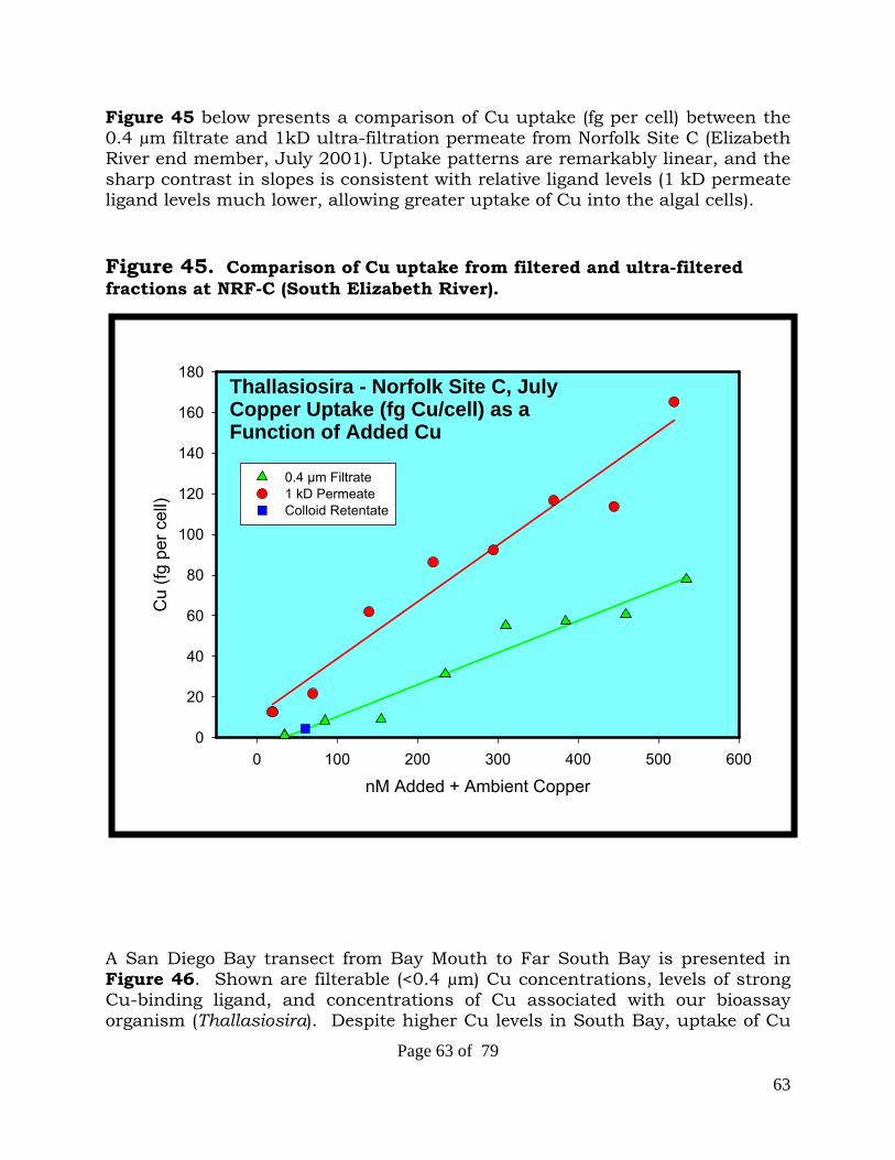
63

Page 63 of 79

Figure 45 below presents a comparison of Cu uptake (fg per cell) between the 0.4 µm filtrate and 1kD ultra-filtration permeate from Norfolk Site C (Elizabeth River end member, July 2001). Uptake patterns are remarkably linear, and the sharp contrast in slopes is consistent with relative ligand levels (1 kD permeate ligand levels much lower, allowing greater uptake of Cu into the algal cells). Figure 45. Comparison of Cu uptake from filtered and ultra-filtered fractions at NRF-C (South Elizabeth River). A San Diego Bay transect from Bay Mouth to Far South Bay is presented in Figure 46. Shown are filterable (<0.4 µm) Cu concentrations, levels of strong Cu-binding ligand, and concentrations of Cu associated with our bioassay organism (Thallasiosira). Despite higher Cu levels in South Bay, uptake of Cu

Thallasiosira - Norfolk Site C, JulyCopper Uptake (fg Cu/cell) as a Function of Added Cu


Cu

(fg p

er c

ell)

0

20

40

60

80

100

120

140

160

180

0.4 µm Filtrate1 kD Permeate Colloid Retentate

64

Page 64 of 79

into Thallasiosira is low, likely reflecting the much greater abundance of strong Cu-binding ligands in South Bay. However, at the mid-Bay Coronado Bridge site, ligand levels are substantially reduced but Cu levels remain relatively high, and as a result Cu uptake by Thallasiosira is significantly enhanced. Similarly for the Bay Mouth site; despite quite low Cu levels, the concentration of bioavailable Cu is actually greater than in South Bay as strong ligand levels are lower than filterable Cu levels. Figure 46. Uptake of Cu by Thallasiosira as a function of filterable Cu concentrations and strong Cu-binding ligand levels along a San Diego Bay transect. Table 4 presents a summary of bioavailability measures at selected field sites as a means to show a few key findings of this aspect of the project.

San Diego Bay Transect

nM (C

u &

Cu-

Liga

nd)

0

10

20

30

40

50

60

70

80

90

fg C

u pe

r Cel

l

0

2

4

6

8

10

12

14

16

18

20

nM Filtrable CunM Strong Cu-Ligandfg/cell Thalassiosira

BayMouth

HarborIsland

CoronadoBridge

MidSouth Bay

FarSouth Bay

65

Page 65 of 79

Measurements of bioavailable copper at the contrasting study sites indicate that (1) the fraction of filterable Cu that is bioavailable is greatest in the San Diego system, and (2) Cu bioavailability is greatly enhanced by ultrafiltration, where up to 75% of ambient Cu is made accessible after ligand level reduction. Table 4. Bioavailable Cu fractions at selected field sites. Figure 47 on the following page illustrates how these data can be placed into a modeling framework with significant predictive power. The working hypothesis is that the levels of strong Cu-binding ligand, L1, (in contrast to weaker L2 and L3 species) regulate metal availability to biological systems (e.g. algal cells). Therefore, when levels of total filterable Cu are less than L1, uptake into cells should be prevented or at least hindered. However, when Cu levels approach or exceed L1, uptake of metals by organisms should be relatively unhindered and cellular metal levels should rapidly increase. Indeed this is what we are observing in the three study systems (refer to Figure 47). If we plot Cu in the probe organism (in this case Thalassiosira, fg per cell) versus excess Cu (i.e. [Cu] > [L1]), we observe a relationship that supports the working hypothesis. Cellular levels of Cu are extremely low until [L1] is saturated, at which point Cu uptake begins to increase dramatically. Remember that the data points in this plot encompass three very different environments (our three impacted harbors), so the predictive power is quite robust. Note that if instead of the strong ligand [L1], the concentration of weak ligand [L2 or L3] is substituted in the above equation; a much poorer relationship is found, therefore reinforcing the concept of strong ligand control.

Site

0.4 m Filtrate 1 kD Permeate

TotalCu (nM)

Bioavailable Cu (nM)

%Bioavailable

Total Cu (nM)


%Bioavailable

NRF-A 16.5 0.33 2.0 11.0 0.50 4.6

NRF-C 34.6 0.37 1.1 19.4 0.42 2.2

SDF02 35.8 7.07 19.7 16.6 11.3 68.3

SDF03 49.1 3.06 6.2 26.1 15.5 59.2

SD09A 9.8 2.97 30.3 6.3 4.74 75.2

CFNC 7.0 0.37 5.3

Site

0.4 m Filtrate 1 kD Permeate

TotalCu (nM)


%Bioavailable

Total Cu (nM)


%Bioavailable

NRF-A 16.5 0.33 2.0 11.0 0.50 4.6

NRF-C 34.6 0.37 1.1 19.4 0.42 2.2

SDF02 35.8 7.07 19.7 16.6 11.3 68.3

SDF03 49.1 3.06 6.2 26.1 15.5 59.2

SD09A 9.8 2.97 30.3 6.3 4.74 75.2

CFNC 7.0 0.37 5.3

66

Page 66 of 79

Figure 47. Copper uptake into cells can be accurately predicted from levels of strong ligand.

Relationship Between Excess Cu and Cu Levels in Organism Probe (Thalassiosira) in Samples fromThree Marine Estuaries

Excess Cu (nM) i.e. [Cu] > [L 1]-180-160-140-120-100 -80 -60 -40 -20 0 20 40

Cu

fg p

er c

ell

0

10

20

30

40

50

60

70

80

90

100

67

Page 67 of 79

XI. High Precision Cu Stable Isotope Ratio Measurements A. Goal and Summary Our objective was to determine whether sources of Copper (Cu) (and in later research, Zinc (Zn)) in DOD-impacted harbors can be identified by unique stable isotopic signatures of these transition metals. Reconstruction and apportionment of historic metal inputs may also be possible from sediment cores if appropriate coring locations can be identified. Our proof-of-principal evaluation was conducted within the context of our much larger study of Cu and Zn speciation and bioavailability. When we initially proposed this hypothesis and effort, we felt that there was a reasonable chance of success and in general the potentially large benefits (both in application deliverables for the DoD and fundamental geochemical processes) outweighed the risks. However, it was certainly true that this was cutting-edge research given that, except for the work of Maréchal et al. (1999) and Gale et al. (1999), that few investigators had even the analytical capabilities to quantify the isotope fractionation, let alone the environmental application. Our group possessed the analytical tools, as well as extensive field study experience, and therefore was in a unique position to test the hypothesis. We initially estimated that it would require 18-24 months to reach preliminary conclusions, and as it turned out, that was close, but somewhat underestimated. In fact it took us roughly 26 months to overcome some quite recalcitrant analytical hurdles and demonstrate the technical feasibility of measuring extremely small stable isotopic ratio variations of copper in some very nasty matrices. This effort was an absolute prerequisite in the research path for determining the viability of using copper isotopic fractionation in the environment to trace sources of the metal. As briefly outlined in the following sections, the first 12 months effort involved ground-breaking work on Cu isotope systematics on the multi-collector, magnetic sector, inductively-coupled plasma mass spectrometer (MC-MS-ICP-MS; Micromass Isoprobe). The bottom-line conclusion from these studies was very encouraging, and that from an instrumental viewpoint, the applied goal was instrumentally technically feasible. We then moved on to developing methods for recovery and cleanup of Cu from complex matrices (marine and estuarine waters and sediments) This work has been particularly challenging given that both isolation/extraction/concentration and cleanup steps must be essentially quantitative (i.e. they must maintain the exact isotopic signature of the source material). It was also determined that a very high degree of cleanup was required because the MC-MS-ICP-MS Cu isotope ratio precision and accuracy was significantly influenced by the presence of other cations/anions in the samples. Though this might sound like a fairly straight forward exercise in good analytical chemistry, the added constraint of maintaining (and demonstrating) endogenous isotope ratios, as it turned-out, was very demanding of time and resources. In the end, however, we believe

68

Page 68 of 79

that we have overcome the technical/analytical hurdles and feel that a pilot-scale field effort is certainly justified. We worked towards that goal with field samples collected in parallel with the speciation/bioavailability samples, and initial data from DoD-impacted samples showed Cu isotopic signatures significantly different than that of reference standards and seawater (Figure 49). That anti-fouling agent-impacted samples should have a different isotope signature is not implausible given the wide range of Cu-isotope fractionation now recognized to exist in nature, and the extreme precision of our methods. In fact it’s very gratifying that after sticking our neck out several years ago, that recent reports in the literature confirm the early work of Maréchal et al. (1999) and suggest that Cu-isotope fractionation is likely to prove to be a powerful new tool for probing geochemical processes and source attribution (Bermin et al. (2006); Chapman et al. (2006); Markl et al. (2006); Maréchal and Albarède. (2002); Zhu et. al, (2002); Coplen, et. al, (2001); Zhu, et. al, (2000). Though certainly a high visibility component of the overall project, the actual planned fiscal commitment to the Cu-isotope component of the project was quite small in comparison to that required for the speciation and bioavailability components. In fact, because of the analytical challenges (now resolved), the actual effort devoted to the Cu-isotope work went well beyond what was planned, and as a result funding and time for a comprehensive evaluation of Cu isotope ratios in all the field samples collected was inadequate. However, the hard development was completed successfully, and the viability of the hypothesis established. Additional work will be required to field validate the extensive isotope effort to date. We believe that with just a few minor exceptions that field estuarine water sites are adequately sampled to date, and that these should provide a great data set representative of in-harbor mixed isotope conditions. In a couple areas we feel the data set could be strengthened: 1. Copper Ore Samples

We have analyzed common major Cu-containing reagents, and although Cu isotope fractionation is apparent (which bodes well for actual ore samples), the provenance of the reagents is unknown. In collaboration with the Geology and Geophysics Departments we have obtained a small selection of common ores, and these remain to be analyzed. However, it is also critical that we identify and sample the current and historic feedstock ores for common Naval and Recreational anti-fouling coatings. We believe that this should be possible using contacts within the Navy, Coating Manufacturers, and Economic Geologist communities.

2. Anti-fouling Paint Samples

In addition to obtaining a more complete collection of “off-the-shelf” anti-fouling paints representative of both Navy and Recreational boat current and historic application, we would approach paint manufacturers for semi-processed materials.

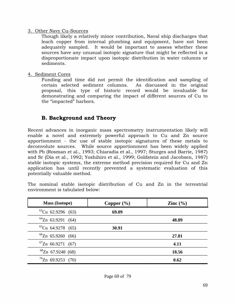
69

Page 69 of 79

3. Other Navy Cu-Sources

Though likely a relatively minor contribution, Naval ship discharges that leach copper from internal plumbing and equipment, have not been adequately sampled. It would be important to assess whether these sources have any unusual isotopic signature that might be reflected in a disproportionate impact upon isotopic distribution in water columns or sediments.

4. Sediment Cores

Funding and time did not permit the identification and sampling of certain selected sediment columns. As discussed in the original proposal, this type of historic record would be invaluable for demonstrating and comparing the impact of different sources of Cu to the “impacted” harbors.

B. Background and Theory Recent advances in inorganic mass spectrometry instrumentation likely will enable a novel and extremely powerful approach to Cu and Zn source apportionment - the use of stable isotopic signatures of these metals to deconvolute sources. While source apportionment has been widely applied with Pb (Rosman et al., 1993; Chiaradia et al., 1997; Sturges and Barrie, 1987) and Sr (Dia et al., 1992; Yoshihiro et al., 1999; Goldstein and Jacobsen, 1987) stable isotopic systems, the extreme method precision required for Cu and Zn application has until recently prevented a systematic evaluation of this potentially valuable method. The nominal stable isotopic distribution of Cu and Zn in the terrestrial environment is tabulated below:

Mass (Isotope) Copper (%) Zinc (%) 63Cu 62.9296 (63) 69.09 64Zn 63.9291 (64) 48.89 65Cu 64.9278 (65) 30.91 66Zn 65.9260 (66) 27.81 67Zn 66.9271 (67) 4.11 68Zn 67.9248 (68) 18.56 70Zn 69.9253 (70) 0.62

of 79

Recent studies by Chapman et al. (2006); Markl et al. (2006); Zhu et al. (2002), Zhu et al. (2000), Maréchal et al. (1999) and Gale et al. (1999) and earlier work by Shields et al. (1965) and Walker et al. (1958), have shown that stable Cu isotope ratios in copper ores vary significantly in nature, and that the potential therefore exists for source discrimination based upon isotopic signature. Isotopic variation of over 9 per mil between various ore bodies has been reported in these studies. Copper is relatively mobile in geologic processes, and through incomplete redox and exchange reactions, isotopic fractionation may occur. In the earliest published paper addressing natural relative isotopic variation in Cu, Walker et al. (1958), using a Nier type mass spectrometer, measured a total spread of -1 to +8 per mil in a number of minerals. Measurement error was estimated to be less than 0.1% using an NBS CuO primary standard and a CuI working standard. Samples (n=12) of chalcocite and native copper from the White Pine mine in Ontonagon Michigan (USA), and samples (n=11) of volborthite, malachite, and azurite from the Cougar mine in Montrose Colorado (USA) were studied along with 16 other samples (including brochantite, pitchblende, marine sediments, niccolite). The sediment sample with the highest positive enrichment contained a large amount of organic matter and was collected in an area with significant anaerobic bacterial activity. The later finding suggests that biologically-mediated redox cycling may enhance isotopic fractionation. The most comprehensive study to date of natural variations in the isotopic composition of Cu, was conducted by Shields et al. (1965). Over 100 samples, including a large selection of primary and secondary Cu-containing minerals (chalcopyrite, bornite, chalcocite, oxides, carbonates, native Cu, tetrahedrite, etc.) were studied. These investigators employed a much improved mass spectrometer compared with that used by Walker et al.(1958), and were able to obtain stable ratios, essentially independent of time as long as the ion current was not decaying. Shields et al. (1965) referenced their ratios to a standard different from that used by Walker et al. (1958), and therefore the absolute fractionation reported (-9.0 to +3.3 per mil) is not directly comparable with Walker’s data (conversion is easy however), but the total range in fractionation observed (12.3 per mil) is remarkably consistent. The authors concluded that variations in Cu isotope fractionation appear to be related to conditions under which a given mineral species forms, with a secondary influence of location. Maréchal et. al. (1999) employed modern plasma-source mass spectrometry to the study of Cu and Zn isotopic fractionation in silicates, ores, and biological materials. These investigators referenced their ratio data to the NIST Cu standard (SRM 976), a convention that we followed in our work. This study is

of 79

especially relevant from the analytical standpoint, in that our analysis (both instrumental and clean-up) protocols incorporate and build upon the detailed work of these investigators. Ratio precision of 20-40 ppm (0.04 per mil) was reported, similar to that revealed on our instrument in preliminary validation studies. Remarkably, these investigators also reported a range in Cu isotope fractionation of Cu ores of about 9 per mil. The smaller number of ores examined (n=9) prevented any definitive conclusion as to the relationship between mineral type and isotopic signature. The work of Gale et al. (1999) is important in at least three major areas: (a) they corroborated earlier studies by demonstrating that stable isotope fractionation of Cu in natural Cu-containing minerals range between -1.63 to +7.71 per mil (b) an exploratory study of the effect of smelting and fire refining on Cu isotopes, suggested that isotopic fractionation does not occur in these processes, therefore preserving the original isotopic signature of the ore. (c) they compared traditional TIMS techniques with state-of-the-art MC-MS-ICP-MS methods (our method of choice) and found comparable natural fractionation. The important initial question to for us to address is whether the background geochemical isotopic signatures of the various study sites are significantly and usefully different than that of DoD and other anthropogenic copper sources. For source apportionment to be successful, a fractionation of >0.4 per mil must be observed between major end-members, given an isotopic ratio precision of 20-40 ppm.

C. Analytical Considerations Ultra-high-precision isotope ratio measurements of Cu and Zn require the use of complex and expensive mass-spectrometry instrumentation. Potentially two classes of technologies can be applied to the analytical challenge: (A) Thermal Ion Mass Spectrometry (TIMS), and Multiple-Collector, Magnetic Sector, Inductively-Coupled Plasma Mass Spectrometry (MC-MS-ICP-MS). The former approach, though still evolving incrementally, is a mature technique, having been used now for several decades. Its primary application has been in systems with 3 or more stable isotopes, where the ionization potential of the element is relatively low, and where, due to radiogenic parents, large natural variations in stable isotopic abundance are found. These elements include: Neodymium (Nd), Lead (Pb), and Strontium (Sr). However, application of TIMS to Cu-isotope systematics is problematic in that the Cu ionization potential is relatively high leading to very poor efficiencies, and double-spike techniques to correct for instrumental isotopic fractionation cannot be applied since only two stable isotopes exist. In addition the TIMS analysis is extremely time-

of 79

consuming, which coupled with the required pre-analysis chemical separations, dramatically limits sample throughput. Instrumentation for the later approach, MC-MS-ICP-MS, has been commercially available for only about 8 years, and it’s only in the last 5 years that as the scientific community recognized the potential of this technique and compelled manufacturers to modify designs and correct deficiencies, that the early promise has been fulfilled. The great advantages of this technique emanate from the argon plasma-front end. The inductively-coupled plasma is a very efficient ionization source, and therefore elements with high ionization potentials can be effectively measured. Also analysis time is shortened and sample preparation simplified over traditional TIMS approaches. One drawback to this method, though not technical in nature, is the high cost of the instrumentation, typically over $750,000. The multi-collector design allows for simultaneous collection of several ion beams, therefore overcoming the precision limitation imposed by plasma “flicker” in single collector instruments. Multi-collector instruments can produce remarkably precise isotope ratio data, in certain systems better than 0.0005% (5 ppm, .005 per mil). This level of precision is more than adequate to expect that stable isotopic fractionation in non-radiogenic element systems can be accurately quantified. Particularly exciting is the potential for 1st and 2nd row transition metals (including Cu), where multiple redox states are the rule, and where biological and geochemical redox cycling may lead to significant isotopic fractionation.

C. Analytical Progress

The nearly 1 million dollar cost of the MC-MS-ICP-MS system purchased by the UW-Madison in early 2000 was funded through non-DOD sources. Our instrument is of a unique design, where the electrostatic focusing sector of traditional double-focusing designs is replaced by a hexapole-collision cell. The hexapole improves transmission over competing designs, thermalizing and focusing the ions, while the integrated collision cell destroys polyatomic species endemic to plasma-based instrumentation, and which would otherwise interfere with analyte mass spectra. The later factor cannot be over emphasized, spectral interference removal is critical for accurate and intercomparable data. The first year of effort in this area of study was dedicated to demonstrating the technical feasibility of measuring extremely small stable isotopic ratio variations of copper. This work was a necessary first step in determining the viability of using copper isotopic fractionation in the environment to trace sources of the metal. These studies involved ground-breaking work on Cu

of 79

isotope systematics on the multi-collector, magnetic sector, inductively-coupled plasma mass spectrometer (Micromass Isoprobe). As mentioned previously, the bottom-line conclusion from these studies was very encouraging, and that from an instrumental viewpoint, the applied goal was technically feasible.

Figure 48. Copper Stable Isotope Ratio Precision: MS-MC-ICP-MS An example of the external precision obtained during one of our standard validation experiments is shown above in Figure 48. Remarkable precision is apparent, with variation not evident until the 4th or 5th decimal place. A per mil standard deviation (1 σ) of 0.022 is calculated, more than an order-of-magnitude better than would be required to resolve the unit per mil variations measured in copper ores (see above). An important, but somewhat cautionary outcome of these studies was the finding that Cu isotope ratio precision and accuracy was significantly influenced by the presence of other cations in the samples. Therefore, we chose a very conservative approach in confronting the next phase of the validation, i.e. isolation and concentration of Cu from complex natural

NBS = - 0.08

Analysis Number0 5 10 15 20 25

dCu

(65/

63)

-0.20

-0.16

-0.12

-0.08

-0.04

0.00

0.04

0.08

0.12

0.16

0.20

NIST = - 0.08

of 79

matrices. Considering the technical complexities of the overall goal, we decided that to dispatch any concerns (either our own, or from external reviewers) about matrix effects, that we would purify samples such that only trace levels of interfering ions remained. Though this might sound like a fairly straight-forward exercise in good analytical chemistry, the added constraint of maintaining (and demonstrating) endogenous isotope ratios, as it turned-out, was more of a challenge than expected. Our focus for much of the remaining project period was to develop methods for recovery and cleanup of Cu from complex matrices without isotopic fractionation (i.e. maintaining exact!!!!! 63/65 ratio). We directed a large portion of this effort towards methods capable of isolating metals from relatively large volumes of marine and estuarine water. a. Extraction: Isolation of Cu and Zn from Seawater Matrix. To allay concerns about isotopic fractionation, the method must be essentially 100% efficient in isolating Cu and Zn, but equally important one must also be able to recovery 100% of the Cu and Zn from the “sorbant”. Some isotopic fractionation is essentially unavoidable so quantitative recovery is critical and also serves as a good predictor of method effectiveness. We tried several approaches including both solid and liquid-liquid extractions. For example: various immobilized ligands (iminodiacetate on polymer backbone (Chelex), other direct solid-phase extractant resins (Eichrom; Diphonix and Monophosphonic). Chelex displayed good efficiency in extraction from seawater, but we were not able to achieve 100% removal from the Chelex, even with an array of common eluants. Eichrom resins showed the opposite problem - poor and irreproducible extraction efficiency of Cu from seawater, but good recovery from the solid phase. All these methods were also plagued by poor efficiency in pre-cleanup (i.e. interfering ions were also extracted with target Cu and Zn). Somewhat discouraged, we then turned to a method first proposed by Wells and Bruland (1998) for isolation of several metals from saline waters. We adapted and modified this method and after several months of experimentation feel confident that this approach will meet our stringent requirements. A brief summary of the technique follows. One must first synthesize the metal-binding ligand (bis(2-hydroxyethyl) dithiocarbamate (HEDC). We did so according to the method of King and Fritz (1985) using ethanolamine, sodium hydroxide, and carbon disulfide dissolved in methanol, followed by careful precipitation of the crude ligand upon addition of 2-propanol. The ligand was subsequently purified and characterized. The clean ligand is added to seawater samples to form a neutrally-charged, polar (water soluble) metal ligand complex. The ligand has high affinity and specificity for Fe, Co, Ni, Cu, Zn, and Cd. The neutral metal complexes are recovered onto a polystyrene-based C-18 resin column. The metal complexes are eluted from the column with an acidic methanol solution. The eluates are

of 79

evaporated to near dryness after addition of nitric acid to destroy the organic ligand, and the residue taken up in 7 N HCl. Near quantitative isolation of the target metals from major ion matrix is achieved in this method. In brief, the major steps in this process are:

Quantitative Extraction of Cu from Complex Matrices 1. Synthesize ligand (HEDC)

2. Purify and characterize 3. Form metal-ligand complex 4. Recover complex on C-18 5. Elute metal from column 6. Destroy residual ligand

7. Take up metals in 7 N HCl b. Clean-up: Separation of Cu from Other Trace Elements: The sample extract is further cleaned-up, and trace elements separated by anion exchange chromatography on AG MP-1 resins. Copper is eluted from the resin with 23 mL of 7 N HCl. Iron and Zn can be subsequently recovered with 2 N HCl and 0.5 N HNO3 respectively. This clean-up and separation method was adapted from work published by Marechal et al. 1999. The HCL eluates are evaporated to dryness and residue taken up in 1% HNO3 for analysis by MC-MC-ICP-MS.

Clean-up and Separation of Cu from other Elements 1. Anion exchange (AG MP-1) chromatography using 7 N HCl

2. Collect fractions, dry down, take up in dilute nitric acid E. Samples for Stable Isotope Analysis a. Bio-fouling Panel Studies We collaborated with Dr. Peter Seligman (SPAWAR/SYSCEN) to evaluate the Cu (and other metals) leached from panels treated with Cu-biofouling paints. Dr. Seligman provided us a series of seawater leachate samples (BRA-640) from which we worked to provide:

i. high precision Cu isotope ratio measurements (after extraction and removal of seawater matrix). ii. comprehensive multi-element measurements on panel extracts. These data will provide a very valuable data set on minor and trace element leaching rates from the panels. In addition these data will likely support our source reconciliation efforts.

of 79

b. Harbor/Estuary Studies One liter and 0.5 liter samples for stable isotope measurements were collected from each of our study sites on every sampling campaign. Since this sampling program focused on the filterable phases, all isotope samples were field filtered through 0.4 µm Meissner polypropylene filters. We have demonstrated that this filter behaves ideally with respect to Cu and Zn, neither sorbing “dissolved” metal nor introducing metal contamination. This behavior is a prerequisite for accurate isotope ratio characterization of the samples. We also collected particulate phases on a 1 µm Teflon membrane for exploratory measurements of stable isotope ratios in suspended particles. Water samples were stabilized with ultra-high purity nitric acid to ensure high metal recovery. The blank contributed by the acid is negligible.

Impacted-Harbor Cu-Isotope Sample Summary (number of samples collected) Cape Fear Dissolved (4) Particulate (4) Colloidal (6) Norfolk Harbor Dissolved (12) Particulate (12) Colloidal (5) San Diego Bay Dissolved (28) Particulate (28) Colloidal (12) In addition to the Harbor/Estuary samples, we obtained the following “source” samples.

Cu Stable Isotope Source Sample Summary Navy ship hull panel leachates (BRA-640) A commercial Cu-based antifouling paint Six Cu ores representing industrial feed stocks Reference seawater Vegetation from Cu mine-impacted area Several rivers draining contrasting watersheds Figure 49 on the following page presents some preliminary Cu-isotope fractionation (signature) data. Though the data set is still small, and we’re not

of 79

yet capable of asserting that our hypothesis is definitive, it is apparent that a large range in isotopic fractionation is exists (more than an order of magnitude greater than our analytical precision) and that impacted-harbor samples are differentiated from selected source samples.

Figure 49. Measured copper stable isotope ratios in selected reference and field samples. F. Citations Bermin J., D. Vance, C. Archer, and P.J. Statham. 2006. The determination of the isotopic composition of Cu and Zn in seawater. Chemical Geology 226:280-297.

Copper Isotope Fractionation

del 65Cu (vs HPS Cu)

-0.5 0.0 0.5 1.0 1.5 2.0 2.5 3.0

White Pine Mine

Copper Salts

Copper Metal

Seawater

NBS 976

BRA-640

Norfolk FD

Norfolk FC

San Diego NF04

San Diego F03

of 79

Chapman J.B., T.F,D. Mason, D.J. Weiss, B.J. Coles, and J.J. Wilkinson. 2006. Chemical separation and isotopic variations of Cu and Zn from five geological reference materials. Geostandards and Geoanalytical Research 30:5-16.

Chiaradia, M., B.E. Chenhall, A.M. Depers, B.L. Gulson, and B.G. Jones. 1997. Identification of historical lead sources in roof dusts and recent lake sediments from an industrialized area: indications from lead isotopes. Sci. Tot. Environ. 205:107-128. Coplen, T.B., J.A. Hopple, J.K. Böhlke, H.S. Peiser, S.E. Rieder, H.R. Krouse, K.J. R. Rosman, T. Ding, R.D. Vocke Jr., K.M. Révész, A. Lamberty, P. Taylor, and P. De Bièvre. 2001. Compilation of Minimum and Maximum Isotope Ratios of Selected Elements in Naturally Occurring Terrestrial Materials and Reagents. USGS Water Resources Investigation Report 01-4222. Dia, A.N., A.S. Cohen, R.K. O’Nions, and N.J. Shakelton. 1992. Seawater Sr isotope variation over the past 300 kyr and influence of global climate cycles. Nature 356:786-788. Gale, N.H., A.P. Woodhead, Z.A. Stos-Gale, A. Walder, and I. Bowen. 1999. Natural variations detected in the isotopic composition of copper: possible applications to archaeology and geochemistry. International Journal of Mass Spectrometry, 184(1):1-9. Goldstein, S.J. and S.B. Jacobsen. 1987. Nd and Sr isotopic systematics of river water dissolved material: implications for the sources of Nd and Sr in seawater. Chem. Geol. 66:245-272. Halliday, A.N., D.C. Lee, J.N. Christensen, M. Rehkamper, W. Yi, X. Luo, C.H. Hall, C.J. Ballentine, T. Pettke, and C. Stirling. 1998. Applications of multiple collector-ICPMS to cosmochemistry, geochemistry, and paleoceanography. Geochimica et Cosmochimica Acta, 62(6):919-940. Maréchal, C.N., and F. Albarède. 2002. Ion-exchange fractionation of copper and zinc isotopes. Geochimica et Cosmochimica Acta, 66(9):1499-1509. Maréchal, C.N., P. Télouk, and F. Albarède. 1999. Precise analysis of copper and zinc isotopic compositions by plasma-source mass spectrometry. Chemical Geology, 156:251-273. Markl, G., Y. Lahaye, and G. Schwinn. 2006. Copper isotopes as monitors of redox processes in hydrothermal mineralization. Geochimica et. Cosmochimica Acta 70:4215-4228.

of 79

Rosman, K.J., W. Chisholm, C.F. Boutron, J.P. Candelone, and U. Gorlach. 1993. Isotopic evidence for the source of lead in Greenland snows since the late 1960s. Nature 362:333-335. Shields, W.R., S.S. Goldich, E.L. Garner, and T.J. Murphy. 1965. Natural variations in the abundance ratio and the atomic weight of copper. Journal of Geophysical Research, 70(2):479-491. Sturges, W.T. and L.A. Barrie. 1987. Lead 206/207 isotope ratios in the atmosphere of North America as tracers of US and Canadian emissions. Nature 329:144-146. Vanhaecke, F., L. Moens, R. Dams, I. Papadakis, and P. Taylor. 1997. Applicability of high-resolution ICP-Mass Spectrometry for isotope ratio measurements. Analytical Chemistry, 69(2):268-273. Walker, E.C., F. Cuttitta, and F.E. Senftle. 1958. Some natural variations in the relative abundance of copper isotopes. Geochimica et Cosmochimica Acta, 15:183-194. Wells, M.L., and K.W. Bruland. 1998. An improved method for rapid preconcentration and determination of bioactive trace metals in seawater using solid phase extraction and high resolution inductively coupled plasma mass spectrometry. Marine Chemistry, 63:145-153. Yoshihiro, A., T. Tsuyoshi, K. Hikari, and N. Akira. 1999. Provenance of the North Pacific sediments and process of source material transport as derived from Rb-Sr isotopic systematics. Chemical Geology 158(3/4):271-291. Zhu, X.K., Y. Guo, R.J.P. Williams, R.K. O’Nions, A. Matthews, N.S. Belshaw, G.W. Canters, E.C. de Waal, U. Weser, B.K. Burgess, and B. Salvato. 2002. Mass fractionation processes of transition metal isotopes. Earth and Planetary Science Letters, 200:47-62. Zhu, X.K., R.K. O’Nions, Y. Guo, N.S. Belshaw, and D. Rickard. 2000. Determination of natural Cu-isotope variation by plasma-source mass spectrometry: implications for use as geochemical tracers. Chemical Geology, 163:139-149.

speciation, sources and bioavailability of copper … sources and bioavailability of copper and zinc...

Documents