specifications and strategies for state estimation of ...470903/fulltext01.pdf · specifications...
TRANSCRIPT
Specifications and strategies for state
estimation of vehicle and platoon
MUHAMMAD ALTAMASH AHMED KHAN
Master’s Degree Project
Stockholm, Sweden August 2011
XR–EE–SB 2011:013

To my Family.

Table of Contents
Table of Contents ii
List of Tables v
List of Figures vi
Nomenclature ix
Abstract xi
Acknowledgements xii
1 Introduction 11.1 Prelude . . . . . . . . . . . . . . . . . . . . . . . . . . . . . . . . . . . . . . . . . . . 11.2 Previous efforts . . . . . . . . . . . . . . . . . . . . . . . . . . . . . . . . . . . . . . . 21.3 Grand Cooperative Driving Challenge (GCDC) . . . . . . . . . . . . . . . . . . . . . 21.4 Work description . . . . . . . . . . . . . . . . . . . . . . . . . . . . . . . . . . . . . . 41.5 Thesis outline . . . . . . . . . . . . . . . . . . . . . . . . . . . . . . . . . . . . . . . . 5
2 Background 62.1 States of a system . . . . . . . . . . . . . . . . . . . . . . . . . . . . . . . . . . . . . 62.2 Reference frames . . . . . . . . . . . . . . . . . . . . . . . . . . . . . . . . . . . . . . 7
2.2.1 Types of reference systems . . . . . . . . . . . . . . . . . . . . . . . . . . . . 72.2.2 Conversion between the reference systems . . . . . . . . . . . . . . . . . . . . 10
2.3 State estimation techniques . . . . . . . . . . . . . . . . . . . . . . . . . . . . . . . . 122.3.1 Kalman filter . . . . . . . . . . . . . . . . . . . . . . . . . . . . . . . . . . . . 132.3.2 Extended kalman filter . . . . . . . . . . . . . . . . . . . . . . . . . . . . . . . 14
2.4 Available sensors . . . . . . . . . . . . . . . . . . . . . . . . . . . . . . . . . . . . . . 162.4.1 GPS . . . . . . . . . . . . . . . . . . . . . . . . . . . . . . . . . . . . . . . . . 162.4.2 Wheel speed sensor . . . . . . . . . . . . . . . . . . . . . . . . . . . . . . . . . 172.4.3 Acceleration sensors . . . . . . . . . . . . . . . . . . . . . . . . . . . . . . . . 182.4.4 Gyro and steering sensor . . . . . . . . . . . . . . . . . . . . . . . . . . . . . 182.4.5 Radar . . . . . . . . . . . . . . . . . . . . . . . . . . . . . . . . . . . . . . . . 19
2.5 GCDC requirements . . . . . . . . . . . . . . . . . . . . . . . . . . . . . . . . . . . . 19
ii
3 Single Vehicle Estimation 223.1 States of a vehicle . . . . . . . . . . . . . . . . . . . . . . . . . . . . . . . . . . . . . 223.2 Kinematic model . . . . . . . . . . . . . . . . . . . . . . . . . . . . . . . . . . . . . . 24
3.2.1 Process model . . . . . . . . . . . . . . . . . . . . . . . . . . . . . . . . . . . 253.2.2 Measurement model . . . . . . . . . . . . . . . . . . . . . . . . . . . . . . . . 31
3.3 Bicycle model . . . . . . . . . . . . . . . . . . . . . . . . . . . . . . . . . . . . . . . . 343.3.1 Process model . . . . . . . . . . . . . . . . . . . . . . . . . . . . . . . . . . . 353.3.2 Measurement model . . . . . . . . . . . . . . . . . . . . . . . . . . . . . . . . 423.3.3 Implementation . . . . . . . . . . . . . . . . . . . . . . . . . . . . . . . . . . . 45
3.4 Covariance matrices . . . . . . . . . . . . . . . . . . . . . . . . . . . . . . . . . . . . 45
4 Platoon Estimation 474.1 States of the platoon vehicle . . . . . . . . . . . . . . . . . . . . . . . . . . . . . . . . 474.2 Separate estimation model . . . . . . . . . . . . . . . . . . . . . . . . . . . . . . . . . 49
4.2.1 Process model . . . . . . . . . . . . . . . . . . . . . . . . . . . . . . . . . . . 494.2.2 Measurement model . . . . . . . . . . . . . . . . . . . . . . . . . . . . . . . . 514.2.3 Relative distance calculation . . . . . . . . . . . . . . . . . . . . . . . . . . . 524.2.4 Vehicle ahead . . . . . . . . . . . . . . . . . . . . . . . . . . . . . . . . . . . . 54
4.3 Joint estimation model . . . . . . . . . . . . . . . . . . . . . . . . . . . . . . . . . . . 544.3.1 Process model . . . . . . . . . . . . . . . . . . . . . . . . . . . . . . . . . . . 554.3.2 Measurement model . . . . . . . . . . . . . . . . . . . . . . . . . . . . . . . . 62
5 Simulation Methodology 645.1 Data acquisition . . . . . . . . . . . . . . . . . . . . . . . . . . . . . . . . . . . . . . 645.2 Kalman filter implementation . . . . . . . . . . . . . . . . . . . . . . . . . . . . . . . 65
5.2.1 Asynchronous sensors data . . . . . . . . . . . . . . . . . . . . . . . . . . . . 665.3 Platoon simulation scenario . . . . . . . . . . . . . . . . . . . . . . . . . . . . . . . . 67
6 Single Vehicle Estimation Results 686.1 Straight run results . . . . . . . . . . . . . . . . . . . . . . . . . . . . . . . . . . . . . 68
6.1.1 Position estimates . . . . . . . . . . . . . . . . . . . . . . . . . . . . . . . . . 696.1.2 Velocities and Speed scale factor estimates . . . . . . . . . . . . . . . . . . . . 716.1.3 Acceleration and Acceleration bias estimates . . . . . . . . . . . . . . . . . . 746.1.4 Yaw angle, Side Slip, Yaw-rate and Yaw-bias estimates . . . . . . . . . . . . . 76
6.2 Turning maneuver results . . . . . . . . . . . . . . . . . . . . . . . . . . . . . . . . . 796.2.1 Position estimates . . . . . . . . . . . . . . . . . . . . . . . . . . . . . . . . . 796.2.2 Velocities and Speed scale factor estimates . . . . . . . . . . . . . . . . . . . . 816.2.3 Acceleration and Acceleration bias estimates . . . . . . . . . . . . . . . . . . 846.2.4 Yaw angle, Side Slip, Yaw-rate and Yaw-bias estimates . . . . . . . . . . . . . 85
6.3 Discussion . . . . . . . . . . . . . . . . . . . . . . . . . . . . . . . . . . . . . . . . . . 89
7 Platoon Estimation Results 907.1 Preface to platoon vehicle estimation . . . . . . . . . . . . . . . . . . . . . . . . . . . 90
7.1.1 Radar modeling . . . . . . . . . . . . . . . . . . . . . . . . . . . . . . . . . . . 927.2 Relative distance . . . . . . . . . . . . . . . . . . . . . . . . . . . . . . . . . . . . . . 927.3 Velocity / Speed . . . . . . . . . . . . . . . . . . . . . . . . . . . . . . . . . . . . . . 95
7.3.1 Absolute speed . . . . . . . . . . . . . . . . . . . . . . . . . . . . . . . . . . . 957.3.2 Relative speed . . . . . . . . . . . . . . . . . . . . . . . . . . . . . . . . . . . 96
7.4 Relative heading (Line bearing) . . . . . . . . . . . . . . . . . . . . . . . . . . . . . . 97
iii

7.5 Acceleration . . . . . . . . . . . . . . . . . . . . . . . . . . . . . . . . . . . . . . . . . 987.6 Discussion . . . . . . . . . . . . . . . . . . . . . . . . . . . . . . . . . . . . . . . . . . 98
8 Conclusion and Future works 1008.1 Conclusion . . . . . . . . . . . . . . . . . . . . . . . . . . . . . . . . . . . . . . . . . 1008.2 Future Work . . . . . . . . . . . . . . . . . . . . . . . . . . . . . . . . . . . . . . . . 101
8.2.1 Inclusion of an IMU . . . . . . . . . . . . . . . . . . . . . . . . . . . . . . . . 1018.2.2 Four wheel model . . . . . . . . . . . . . . . . . . . . . . . . . . . . . . . . . . 1018.2.3 Longer data set . . . . . . . . . . . . . . . . . . . . . . . . . . . . . . . . . . . 1018.2.4 More advanced platoon estimation models . . . . . . . . . . . . . . . . . . . . 1018.2.5 Real time implementation and testing . . . . . . . . . . . . . . . . . . . . . . 101
Bibliography 102
iv

List of Tables
3.1 Definition of the notations used in the F matrix . . . . . . . . . . . . . . . . . . . . 31
3.2 Measurement noise co-variance matrix Rk . . . . . . . . . . . . . . . . . . . . . . . . 46
4.1 Definition of the notations used in the F matrix . . . . . . . . . . . . . . . . . . . . 51
4.2 Definition of the notations used in the F matrix . . . . . . . . . . . . . . . . . . . . 61
5.1 Truck parameters . . . . . . . . . . . . . . . . . . . . . . . . . . . . . . . . . . . . . . 65
v

List of Figures
1.1 Cooperative driving [1] . . . . . . . . . . . . . . . . . . . . . . . . . . . . . . . . . . 3
2.1 Rectangular ECEF reference system [2] . . . . . . . . . . . . . . . . . . . . . . . . . 8
2.2 Geodetic ECEF reference system . . . . . . . . . . . . . . . . . . . . . . . . . . . . . 9
2.3 Local geodetic or tangent reference system . . . . . . . . . . . . . . . . . . . . . . . . 9
2.4 Body frame reference system . . . . . . . . . . . . . . . . . . . . . . . . . . . . . . . 10
2.5 GPS receivers . . . . . . . . . . . . . . . . . . . . . . . . . . . . . . . . . . . . . . . . 17
2.6 Steering wheel angle vs Wheel steering angle . . . . . . . . . . . . . . . . . . . . . . 19
3.1 Dynamic model for vehicle [3] . . . . . . . . . . . . . . . . . . . . . . . . . . . . . . . 23
3.2 Scania’s test track . . . . . . . . . . . . . . . . . . . . . . . . . . . . . . . . . . . . . 25
3.3 Bicycle model for vehicle [4] . . . . . . . . . . . . . . . . . . . . . . . . . . . . . . . . 35
3.4 Lateral force vs the tyre slip angle [5] . . . . . . . . . . . . . . . . . . . . . . . . . . 37
3.5 Bicycle model implementation . . . . . . . . . . . . . . . . . . . . . . . . . . . . . . . 45
4.1 Vehicles forming a platoon [1] . . . . . . . . . . . . . . . . . . . . . . . . . . . . . . . 48
4.2 Separate estimation model representation . . . . . . . . . . . . . . . . . . . . . . . . 49
4.3 Description of relative states . . . . . . . . . . . . . . . . . . . . . . . . . . . . . . . 53
4.4 Platoon vehicles acting like spring mass System [6] . . . . . . . . . . . . . . . . . . . 55
5.1 Time line with the sensor data . . . . . . . . . . . . . . . . . . . . . . . . . . . . . . 65
5.2 Measurement update step . . . . . . . . . . . . . . . . . . . . . . . . . . . . . . . . . 67
6.1 Estimated trajectory using the EKF with bicycle model . . . . . . . . . . . . . . . . 69
6.2 Number of visible satellites . . . . . . . . . . . . . . . . . . . . . . . . . . . . . . . . 69
6.3 Innovation sequence east . . . . . . . . . . . . . . . . . . . . . . . . . . . . . . . . . . 70
6.4 Innovation sequence north . . . . . . . . . . . . . . . . . . . . . . . . . . . . . . . . . 70
6.5 Innovation sequence up . . . . . . . . . . . . . . . . . . . . . . . . . . . . . . . . . . 71
vi

6.6 Longitudinal velocities comparison . . . . . . . . . . . . . . . . . . . . . . . . . . . . 72
6.7 Speed scale factor . . . . . . . . . . . . . . . . . . . . . . . . . . . . . . . . . . . . . . 72
6.8 Longitudinal velocity innovation sequences . . . . . . . . . . . . . . . . . . . . . . . . 73
6.9 Lateral velocity . . . . . . . . . . . . . . . . . . . . . . . . . . . . . . . . . . . . . . . 73
6.10 Vertical velocity . . . . . . . . . . . . . . . . . . . . . . . . . . . . . . . . . . . . . . . 74
6.11 Longitudinal acceleration . . . . . . . . . . . . . . . . . . . . . . . . . . . . . . . . . 74
6.12 Lateral acceleration . . . . . . . . . . . . . . . . . . . . . . . . . . . . . . . . . . . . . 75
6.13 Lateral accelerometer bias . . . . . . . . . . . . . . . . . . . . . . . . . . . . . . . . . 75
6.14 Yaw angle / Heading . . . . . . . . . . . . . . . . . . . . . . . . . . . . . . . . . . . . 76
6.15 Side slip angle . . . . . . . . . . . . . . . . . . . . . . . . . . . . . . . . . . . . . . . . 76
6.16 Yaw angle innovation sequences . . . . . . . . . . . . . . . . . . . . . . . . . . . . . . 77
6.17 Yaw rate . . . . . . . . . . . . . . . . . . . . . . . . . . . . . . . . . . . . . . . . . . . 77
6.18 Yaw rate gyro bias . . . . . . . . . . . . . . . . . . . . . . . . . . . . . . . . . . . . . 78
6.19 Wheel steering angle . . . . . . . . . . . . . . . . . . . . . . . . . . . . . . . . . . . . 78
6.20 Estimated trajectory using the EKF with bicycle model . . . . . . . . . . . . . . . . 79
6.21 Estimated trajectory using the EKF with kinematic model . . . . . . . . . . . . . . . 79
6.22 Innovation sequence east . . . . . . . . . . . . . . . . . . . . . . . . . . . . . . . . . . 80
6.23 Innovation sequence north . . . . . . . . . . . . . . . . . . . . . . . . . . . . . . . . . 80
6.24 Innovation sequence up . . . . . . . . . . . . . . . . . . . . . . . . . . . . . . . . . . 81
6.25 Longitudinal velocities comparison . . . . . . . . . . . . . . . . . . . . . . . . . . . . 81
6.26 Speed scale factor . . . . . . . . . . . . . . . . . . . . . . . . . . . . . . . . . . . . . . 82
6.27 Longitudinal velocity innovation sequences . . . . . . . . . . . . . . . . . . . . . . . . 82
6.28 Lateral velocity . . . . . . . . . . . . . . . . . . . . . . . . . . . . . . . . . . . . . . . 83
6.29 Vertical velocity . . . . . . . . . . . . . . . . . . . . . . . . . . . . . . . . . . . . . . . 83
6.30 Longitudinal acceleration . . . . . . . . . . . . . . . . . . . . . . . . . . . . . . . . . 84
6.31 Lateral acceleration . . . . . . . . . . . . . . . . . . . . . . . . . . . . . . . . . . . . . 84
6.32 Lateral accelerometer bias . . . . . . . . . . . . . . . . . . . . . . . . . . . . . . . . . 85
6.33 GPS heading . . . . . . . . . . . . . . . . . . . . . . . . . . . . . . . . . . . . . . . . 85
6.34 Heading / Yaw angle estimates . . . . . . . . . . . . . . . . . . . . . . . . . . . . . . 86
6.35 Side slip angle . . . . . . . . . . . . . . . . . . . . . . . . . . . . . . . . . . . . . . . . 86
6.36 Yaw angle innovation sequences . . . . . . . . . . . . . . . . . . . . . . . . . . . . . . 87
6.37 Yaw rate . . . . . . . . . . . . . . . . . . . . . . . . . . . . . . . . . . . . . . . . . . . 87
6.38 Yaw rate gyro bias . . . . . . . . . . . . . . . . . . . . . . . . . . . . . . . . . . . . . 88
6.39 Wheel steering angle . . . . . . . . . . . . . . . . . . . . . . . . . . . . . . . . . . . . 88
7.1 Platoon trajectory . . . . . . . . . . . . . . . . . . . . . . . . . . . . . . . . . . . . . 91
vii

7.2 Time headway . . . . . . . . . . . . . . . . . . . . . . . . . . . . . . . . . . . . . . . 91
7.3 Relative distance components for vehicle no. 2 ∆p21e and ∆p21n . . . . . . . . . . . . 92
7.4 Relative distance components for vehicle no. 3 ∆p31e and ∆p31n . . . . . . . . . . . . 93
7.5 Relative distance to the vehicle no. 2 ∆d12 . . . . . . . . . . . . . . . . . . . . . . . 93
7.6 Difference of relative distances with radio outage and without outage, Vehicle No.2 94
7.7 Relative distance to the vehicle no. 3 ∆d13 . . . . . . . . . . . . . . . . . . . . . . . 94
7.8 Difference of relative distances with radio outage and without outage, Vehicle No.3 95
7.9 Absolute speed of vehicles . . . . . . . . . . . . . . . . . . . . . . . . . . . . . . . . . 95
7.10 Relative speed of vehicles, east component . . . . . . . . . . . . . . . . . . . . . . . . 96
7.11 Relative speed of vehicles, north component . . . . . . . . . . . . . . . . . . . . . . . 96
7.12 Relative speed of vehicles . . . . . . . . . . . . . . . . . . . . . . . . . . . . . . . . . 97
7.13 Relative bearing of vehicles . . . . . . . . . . . . . . . . . . . . . . . . . . . . . . . . 97
7.14 Absolute acceleration of vehicles . . . . . . . . . . . . . . . . . . . . . . . . . . . . . 98
viii

Nomenclature
β Side slip angle
η Speed scale factor
λ Longitude
ν Heading
ω Yaw-rate
φ Latitude
ψ Yaw angle
θ Pitch angle
ϕ Roll angle
ax Longitudinal component of acceleration in body frame
ay Lateral component of acceleration in body frame
bω Yaw-rate gyro bias
bay Lateral accelerometer bias
pe East coordinate of position in ENU frame
pn North coordinate of position in ENU frame
pu Up coordinate of position in ENU frame
vd Vertical component of velocity in ENU frame
vG Ground component of velocity in ENU frame
ix
vx Longitudinal component of velocity in body frame
vy Lateral component of velocity in body frame
Xk State vector at time instant k
Yk Observation vector at time instant k
ADAS Advanced driver assistance systems
ADASE Advanced driving assistance system in europe
DARPA-GC Defense advanced research projects agency - Grand challenge
ECEF Earth centric earth fixed
ENU East-North-Up
GCDC Grand cooperative driving challenge
x

Abstract
Advancement in the automobile industry has resulted in the concept of advanced driver assistance
systems (ADAS). As of now, a major portion of ADAS is essentially non-cooperative in nature. These
systems make use of the information gathered by in-car sensors that scan the vehicle’s environment.
Significant progress can be made, however, when vehicles not only sense information, but also
communicate intelligently with other vehicles and road side infrastructure. This constitutes the field
of cooperative driving which was the objective of the Grand Cooperative Driving Challenge (GCDC)
competition, held in May 2011 at Helmond, Holland.
The purpose of this thesis is to define specifications and strategies, that could be employed for the
state estimation of single vehicle and of a platoon of vehicles, specifically for the GCDC competition.
The states of a vehicle are the parameters that can be used in navigation and control of a vehicle.
In the current thesis work, it includes the parameters transmitted to other platoon vehicles as well
as the those sent to vehicle’s controller. Two types of states have been classified, namely the single
vehicle states and the platoon states. Different models have been studied for the representation of
single vehicle and the vehicles in the platoon. Each model has its own particular advantages and
disadvantages. The decision of employing a model depends upon the platooning strategies, and the
processing power available. Kalman filters have been used for the state estimation.
xi
Acknowledgements
I would like to express my sincere gratitude to my supervisors Dennis Sundman and Henrik Petters-
son and to my examiner Magnus Jansson, for their continuous help and guidance, with out which
this work would not have been possible.
It was a genuine pleasure to work with the Scoop team: Joakim Kjellberg, Elin Stalklinga,
Liliana Garcia, Mattias Bjork, Mohammadreza Khaksari, Sagar Behere and Simon Pettersson, whose
commitment to the task was exemplary. All members were highly helpful and cooperative, and i
thoroughly enjoyed working with them. It was a great learning experience for me. Specially, the
able leadership of Jonas Martensson was quite essential to the over all success of this project. Also,
i am highly grateful to Rickard Lyberger for his kindness and support.
I would also like to acknowledge Assad Al Alam, John-Olof Nilsson and Dave Zachariah for their
generous help and advice. I always found them willing to discuss, even stupidest of my ideas.
My final words go to my family, whose love and guidance have been elementary to all achievements
in my life.
xii

Chapter 1
Introduction
1.1 Prelude
Man has always been in search of ease and convenience. For most part of the history, human modes
of travel have been in-efficient and time consuming . They were not only physically exhaustive, but
were also a major co-factor in the slow economic progress of the societies. As the his knowledge of
nature increased, man eagerly learned to harness its maverick forces, for own benefits. The discovery
of the enormous power of steam was not a different story, as it was quickly learned, how to make
good use of it. Steam engines were designed, which were used in the early rail locomotives. But
human ingenuity did not stop here, as it was instantly realized that same principle could be used to
draw wheeled carts. This gave birth to the early forms of road vehicles.
Since the dawn of automotive travel, it has been the man’s desire to take this new technology to
ever new heights. Research endeavors in the field of automobiles has resulted in the development of
advanced driver assistance systems (ADAS). One of its main purpose is to automate major driving
tasks, hence reducing driver’s work load. As of now, a major portion of ADAS is essentially non-
cooperative in nature. These systems make use of the information that is gathered by on-board
sensors, which scan the vehicle’s environment. Significant progress can be made, when vehicles
not only sense information, but also communicate intelligently with other vehicles and road side
infrastructure. This constitutes the field of cooperative driving, in which the vehicles on the road
communicate with each other, resulting in better collective behavior. Its effect can be realized as the
increased throughput on the road and improved safety. The information gathered in this way can
help drivers and vehicle-systems make better judgments, resulting in smoother and safer driving.
1

2
Smoother driving decreases congestion problems, resulting in lower fuel consumption and lower
CO2 emission. Communication between vehicles is a step along the path towards the ideal of a truly
intelligent transport system. This was the objective of grand cooperative driving challenge (GCDC),
held in May 2011 at Helmond, Holland, that aimed to accelerate the development, integration,
demonstration and deployment of cooperative driving systems.
1.2 Previous efforts
There have been numerous efforts made in the development of driver assistance systems. Some of the
work has been done in the field of autonomous driving like the defense advanced research projects
agency, grand challenge (DARPA-GC) project. The (DARPA-GC) project is a research program
that aims at developing technology to automate the vehicular mode of travel and transportation in
order to keep the troops out of danger. DARPA project includes the vehicles traveling in multiple
real life environment like build up areas and urban cities. Its objective is to simulate the miliary
supply missions with the vehicles making their way through the haze of city traffic, passing through
the streets safely.
While DARPA-GC project is specifically focused towards military’s need of a fully autonomous
driving system, some other work has been done in scope of civilian assisted driving like advanced
driving assistance system in Europe (ADASE II). ADASE II is a joint European research platform for
research in field of advanced driving assistance. It aims at improving the transport safety, efficiency
and comfort without using extra resources in terms of energy or special infra structure. ADASE II
uses a combination of recent automobile technologies complemented by the telemetric links to traffic
management centers, other vehicles and service providers. The vehicle receives information about
the terrain and the traffic lying ahead, which can be used to assist the driver in his tasks or even to
control the vehicle independently.
1.3 Grand Cooperative Driving Challenge (GCDC)
GCDC cooperative ADAS scenarios were envisioned with vehicle moving in platoons. A platoon
is a group of vehicles, moving on the road, sharing the information of mutual interest with each
other. Platooning, in theory, can significantly increase road capacity due to allowing a smaller time

3
headways (the distance between a follower and a leading vehicle divided by follower speed) meanwhile
maintaining a high level of traffic safety. A bottleneck in achieving a smaller time headway, is the
driver’s reaction time. This can be of particular concern at high speeds, when a delay in the response
can lead to a disaster. Therefore, the driver style adaptation is not the solution. adaptive cruise
control (ACC) was introduced some years ago, to address the problem. ACC systems try to achieve
and maintain specified time headways, using environmental sensors - radar, lidar or even vision based
systems - that measure the distance and relative velocity between the ACC-equipped vehicle and
the preceding vehicle. Vehicles acceleration and deceleration is automatically adjusted, based on the
input from these sensors. This leaves the driver with the control of steering only. Time headways
that can be achieved with the ACC systems, ranges between 1s to 3s. It has been theorized that
with the application of ACC systems at short headways may lead to unstable traffic behavior, known
as string instability, i.e. amplification of disturbances in the upstream direction. A short braking
action of a vehicle will introduce a disturbance in the platoon of vehicles, causing a shockwave that
amplifies in the upstream direction, finally leading to a full stand-still of follower vehicles at some
point or even to a collision.
Figure 1.1: Cooperative driving [1]
A solution based upon the mobile communication technology has been suggested to alleviate
this problem. In such an approach, the vehicles share their dynamic information such as position,
velocity and acceleration with each other. In this manner a ”look further ahead” scenario can be
realized, in which the vehicles can know the condition of many preceding vehicles . In this way

4
stable platoon behavior can be achieved, while maintaining a relatively short headway time. The
system created by the combination of the ACC-like controllers with wireless communication (vehicle-
to-vehicle (V2V) communication and vehicle-to-infrastructure (V2I) communication) is commonly
known as cooperative adaptive cruise control (CACC).
A main challenge in the large scale deployment of CACC is the serviceability and reliability of
the system. This requires the design of the system to be made fail safe, comprising of redundant
solutions to ensure safety in case of system’s failure.
The main concepts of GCDC 2011 was to test the working of a CACC system. It comprised
of a GCDC lead vehicle, competing vehicles from different teams and road side facilities. This
provided the participants with a realistic environment to test and demonstrate their innovative
solutions for cooperative driving. The aforementioned issue of string stability was also tested during
different phases of competition. There were two distinct phases of the competition, a simulated
urban phase and a highway phase. The urban phase featured traffic lights and road side units. In
highway phase, the traffic consisted of sets of platoons, separated by relatively large inter platoon
distances, compared to the short intra platoon distances (small time headways). This posed specific
communication and control challenges. Therefore, both intra platoon behavior and inter platoon
behavior (joining another platoon) were evaluated in the GCDC 2011 competition. Platooning is
not limited to highway scenarios. In urban situations, there are significant advantages of platooning
capabilities. The acceleration behavior at traffic lights, where platooning technology will help to
maximize the throughput at green lights is an example of such a situation. [1]
1.4 Work description
This thesis work is a part of the Scoop project, which was a joint effort of Kungliga Tekniska
Hogskolan (KTH) and Scania CV AB. It intended to develop a vehicle control system for the GCDC
2011. Specifically, the thesis aims at studying different strategies that can be employed for the state
estimation of the own vehicle, also referred as the ego vehicle, and of the platoon. The states of
the vehicles are the parameters that are necessary for navigation and control the vehicle. State
estimation depends upon the raw input data from various sources, both from own vehicle and from
other members of the platoon. They are dubbed as observations, which are related to the states
5
being estimated. Observations are often tempered by random biases and noises, which may be
time varying in nature and therefore cannot be used directly. This leads to the requirement of some
method that merges the data from various sensors together, to form a integrated and reliable picture
of the dynamic system. The most commonly used method for fusing the motley data, is the kalman
filter. Kalman filter optimally fuses data from varies sensors using mathematical models to produce
state estimates that are theoretically the best realization of actual state values. Two models each for
single vehicle estimation and platoon vehicles estimation have been studied in the course of thesis
work. Each model has its advantages and disadvantages. Tuning is necessary for kalman estimator
in order to achieve the optimal results.
1.5 Thesis outline
The structure of the report is described below
1. Introduction
2. Background
3. Ego Vehicle Estimation
4. Platoon Vehicle Estimation
5. Simulation Methodology
6. Single Vehicle Estimation Results
7. Platoon Estimation Results
8. Conclusion and Future Work
9. Bibliography

Chapter 2
Background
This chapter briefly describes the states of vehicles, available raw data, principles behind the state
estimation, and the GCDC requirements. The first section of the chapter overviews the formal
description of the states of the vehicle. In the next part of the chapter, attention is given to the
methods employed for the state estimations. Then, the data available to calculate those states is
mentioned and in the last part, the requirements laid out by GCDC organization are described.
2.1 States of a system
The key to analyze any physical system is to mathematically model it. A physical system can be
modeled as either being static or dynamic. Static system is one that can be fairly modeled by a
set of constant parameters. An example of a static system include constant stress forces acting on
the building structures. Dynamic systems, on the other hand are modeled by a set of variables
that describe their status. That status is normally defined in terms of so called state variables,
which are usually a function of time. Examples of dynamic systems include a swinging pendulum,
a moving vehicle, a biological system etc. From practical standpoint, almost all of the systems
occurring in nature or man-made are dynamic in essence. Static systems are defined as static under
some particular constraint. Further classification of systems can be made on their nature, that can
be either continuous or discrete. All naturally occurring systems are continuous but for ease of
analysis, they can be discretized. In this thesis, discrete systems are the focus of study.
The states of a system are the variables that can be used to represent , analyze or control a system.
6
7
Normally these states are described by set of equations that tell sufficient information which can be
used to predict the future behavior of the system. Equations that describes the progression /change
of state variables w.r.t. the time, represented as Xk, are called state equations. There is also a
second set of equations, that relates states variables to the physical observations represented as Yk.
They are called observation or measurement equations. Together, Xk and Yk, form the state space
model or representation for the system of interest. While most of the states are directly observable,
some other are not. They referred to as the hidden states of the system.
A vehicle may be considered as a dynamic system. Typical vehicular states are position, velocity,
acceleration, normal and frictional forces, side slip, bank angle, pitch angle etc.
2.2 Reference frames
The main purpose of this thesis work is to develop a estimator module that estimates the dynamic
states of the vehicle. Usually these states are defined in different reference frames. A frame of refer-
ence is a term used to describe a coordinate system with respect to which the position, orientation,
and other properties of an object are defined. Therefore a knowledge of different types of frames of
references, also called coordinate systems and their inter conversion, is required before proceeding
any further.
2.2.1 Types of reference systems
In the following sub-sections, four types of reference frames will be discussed. First one is the inertial
frame. The second type is called earth centric earth fixed (ECEF) reference system. Third type
is the local geodetic or tangent reference systems and the fourth one is the body vehicle reference
frame. A state variable x defined in a reference frame a is referred to as xa. Description of these
reference frames is given is the subsection 2.2.1.
Inertial reference system
Inertial reference frame is the one in which Newton’s laws of motion hold true, [2, p.46]. Therefore
it is a frame that is at rest or is in continuous motion with constant speed. Its origin can be at

8
arbitrary location. Its cardinal axis are mutually perpendicular to each other. Output from the
inertial sensors is normally described in this reference frame resolved with respect to the body frame
in which the sensor is physically present.
ECEF reference system
ECEF stands for earth centric earth fixed reference system. ECEF frame has its origin at the
center of the earth. It rotates with the earth such that any point on the surface of the earth can
be mapped uniquely in this reference system. Global positioning system (GPS) measurements are
made in this reference frame. It has two sub coordinate systems that can be used to tag a point,
namely rectangular ECEF frame and geodetic ECEF frame.
Rectangular ECEF reference system A point P in rectangular ECEF reference system can
be represented by three cartesian coordinates mentioned as [x, y, z]e. Its x-axis passes through the
point of intersection of great circle passing through two poles also called prime meridian and the
equator. Its z-axis passes through the true North and y-axis completes the right hand rotation and
passes through the equator at 90 degrees. This is shown in figure 2.1,
Figure 2.1: Rectangular ECEF reference system [2]
Geodetic ECEF reference system Another way of tagging points in ECEF reference system is
by approximating the earth as an ellipsoid and then assigning the point of interest P on its surface a
3- tuple ( φ, λ, h). Here φ is termed as the latitude, λ as longitude and h as the altitude of the point
P. Latitude is defined as angle in the meridian plane, from the equatorial plane to the ellipsoidal

9
normal at the point P. The longitude is the angle in the equatorial plane, from the prime meridian
to the the projection of the point of interest P on the equatorial plane. This is shown in the figure
2.2,
Figure 2.2: Geodetic ECEF reference system
Local geodetic or Tangent reference system
It is usually termed as East-North-Up (ENU) reference system. It can be determined by fitting a
tangent plane to the earth’s reference geoid at the point of interest P. Its x-axis points towards east,
y-axis points towards the true north while z-axis points towards the upward from the surface of the
earth to complete the rotation. It is show in the figure 2.3,
Figure 2.3: Local geodetic or tangent reference system
For the systems that are stationary and located at the origin of the tangent frame, tangent frame
and the geographical frames actually coincide. For the mobile systems, the origin of the tangent
10
frame is fixed while the origin of the geographical frame moves with the system. Tangent frame
is used for the navigation with respect to some fixed reference such as the runways. Geographical
frame is used to make measurement on the mobile platforms like measuring the relative distance
and speed from the radar mounted on the moving vehicle.
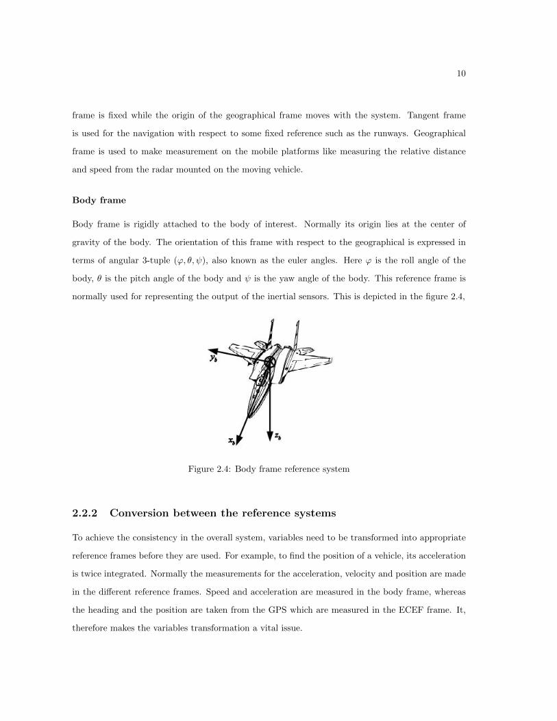
Body frame
Body frame is rigidly attached to the body of interest. Normally its origin lies at the center of
gravity of the body. The orientation of this frame with respect to the geographical is expressed in
terms of angular 3-tuple (ϕ, θ, ψ), also known as the euler angles. Here ϕ is the roll angle of the
body, θ is the pitch angle of the body and ψ is the yaw angle of the body. This reference frame is
normally used for representing the output of the inertial sensors. This is depicted in the figure 2.4,
Figure 2.4: Body frame reference system
2.2.2 Conversion between the reference systems
To achieve the consistency in the overall system, variables need to be transformed into appropriate
reference frames before they are used. For example, to find the position of a vehicle, its acceleration
is twice integrated. Normally the measurements for the acceleration, velocity and position are made
in the different reference frames. Speed and acceleration are measured in the body frame, whereas
the heading and the position are taken from the GPS which are measured in the ECEF frame. It,
therefore makes the variables transformation a vital issue.

11
For illustration purpose, a vectored velocity Vb is assumed to be measured in the body frame
having components Vbx , Vby and Vbz. The transformation of velocity Vb into the geographical or
local tangent frame velocity Vg requires the knowledge of euler angles of the body ϕ , θ and ψ at
the moment of interest. The transformed vector Vg will have components Ve , Vn and Vu. Ve is
the east Component, Vn is the north component and Vu is the up component of the velocity in the
geographical or local tangent frame. The Vg and Vb are related by the equation 2.1,
Vg = Rgb Vb. (2.1)
Here Rgb is the transformation matrix from the body frame to the geographical frame and is given
by equation 2.2,
Rgb =
sψcθ cψcϕ+ sψsθsϕ −cψsϕ+ sψsθcϕ
cψcθ −sψcϕ+ cψsθsϕ sψsϕ+ cψsθcϕ
−sθ cθsϕ cθcϕ
(2.2)
where c stands for the cosine and s for the sine of the angle.
It is common to have the position of the vehicle expressed in the local tangent plane. The reason
for doing so is that the position update in this system only requires the distances traveled by the
body along three locally defined orthogonal axis east, north and up. These distances can be found
by integrating the velocities Ve , Vn and Vu w.r.t. the time. For converting the local ENU position
to the ECEF position, origin of the local tangent plane has to be known. If the origin is represented
by [x0, y0, z0]e in ECEF , then the coordinates of the moving object [pe, pn, pu]t in ENU frame can
be converted to the ECEF position [xe, ye, ze]e , as given in the equation 2.3,
xeyeze
=
x0y0z0
+Ret
pepnpu
. (2.3)
In the equation 2.3 Ret is the transformation matrix from the local tangent plane to the ECEF
plane. It is given by equation 2.4,

12
Ret =
−sin(λ0) −sin(φ0)cos(λ0) cos(φ0)cos(λ0)
cos(λ0) −sin(φ0)sin(λ0) cos(λ0)sin(φ0)
0 cos(φ0) sin(λ0).
(2.4)
where, φ0 and λ0 are the latitude and longitude of the origin of the local tangent plane. Con-
versely, a position vector in rectangular ECEF frame can be converted to the ENU frame. Conversion
equation in that case is shown is equation 2.5
pepnpu
= Rte
xe − x0ye − y0ze − z0
(2.5)
where Rte is the transpose of Ret .
There is often a need to convert coordinates of a point expressed in Geodetic ECEF frame to the
Rectangular ECEF frame. This is normally the case of converting the latitude and longitude mea-
sured by the GPS receiver that are expressed in WGS-84 geodetic system to cartesian coordinates.
The conversion is given by equations 2.6-2.8,
xe = (RN + h)cos(φ)cos(λ) (2.6)
ye = (RN + h)cos(φ)sin(λ) (2.7)
ze = (RN (1− e2) + h)sin(φ) (2.8)
2.3 State estimation techniques
A general definition of a dynamic system was presented in section 2.1. Also as described, the
state space representation for a dynamic system requires the knowledge of state and measurement
equations. State equations are collectively referred to as process model and measurement equations
as the observation model. These two models have to be defined for the analysis of a system, also called
system state estimation. There are many techniques available for the state estimation amongst which

13
kalman filter(KF) is the most popular one. KF is an optimal state estimation algorithm for linear
systems in which the states and the measurements are corrupted by noises. Another derivative of the
Kalman filter is called extended kalman filter(EKF), that is typically used for the state estimation
of non-linear systems. Since the very start, Kalman filter has been the focus of research in the field
of positioning and navigation. A detailed description of the KF theory is beyond the scope of this
report. Instead a brief summary of KF and EKF will be presented in the section below.
2.3.1 Kalman filter
A linear discrete time system is assumed having state vector X ∈ Rm and observation vector
Y ∈ Rn. The state space representation of this system is given by the equations 2.9 and 2.10,
Xk = Fk Xk−1 +Bk Uk−1 + nk (2.9)
Yk = Hk Xk + ek. (2.10)
where,
Xk is the vector of state variables at time instant k
Xk−1 is the vector of state variables at time instant k-1
Yk is the vector of observation variables at time instant k
Fk is the state propagation matrix
Uk is the control input vector to the system
Bk is the input matrix
Hk is the observation matrix
nk is the state or process noise
ek is the measurement or observation noise
14
Vectors nk and ek are assumed to be zero-mean, uncorrelated, white Gaussian noises with co-
variance matrices Qk and Rk respectively.
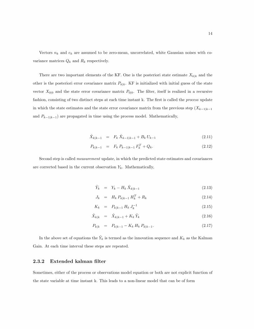
There are two important elements of the KF. One is the posteriori state estimate Xk|k and the
other is the posteriori error covariance matrix Pk|k. KF is initialized with initial guess of the state
vector X0|0 and the state error covariance matrix P0|0. The filter, itself is realized in a recursive
fashion, consisting of two distinct steps at each time instant k. The first is called the process update
in which the state estimates and the state error covariance matrix from the previous step (Xk−1|k−1
and Pk−1|k−1) are propagated in time using the process model. Mathematically,
Xk|k−1 = Fk Xk−1|k−1 +Bk Uk−1 (2.11)
Pk|k−1 = Fk Pk−1|k−1 FTk +Qk. (2.12)
Second step is called measurement update, in which the predicted state estimates and covariances
are corrected based in the current observation Yk. Mathematically,
Yk = Yk −Hk Xk|k−1 (2.13)
Jk = Hk Pk|k−1 HTk +Rk (2.14)
Kk = Pk|k−1 Hk J−1k (2.15)
Xk|k = Xk|k−1 +Kk Yk (2.16)
Pk|k = Pk|k−1 −Kk Hk Pk|k−1. (2.17)
In the above set of equations the Yk is termed as the innovation sequence and Kk as the Kalman
Gain. At each time interval these steps are repeated.
2.3.2 Extended kalman filter
Sometimes, either of the process or observations model equation or both are not explicit function of
the state variable at time instant k. This leads to a non-linear model that can be of form
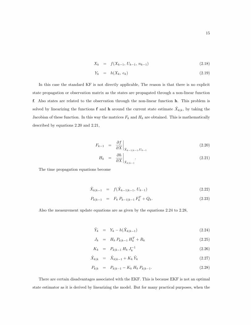
15
Xk = f(Xk−1, Uk−1, nk−1) (2.18)
Yk = h(Xk, ek) (2.19)
In this case the standard KF is not directly applicable, The reason is that there is no explicit
state propagation or observation matrix as the states are propagated through a non-linear function
f. Also states are related to the observation through the non-linear function h. This problem is
solved by linearizing the functions f and h around the current state estimate Xk|k, by taking the
Jacobian of these function. In this way the matrices Fk and Hk are obtained. This is mathematically
described by equations 2.20 and 2.21,
Fk−1 =∂f
∂X
∣∣∣∣Xk−1|k−1,Uk−1
(2.20)
Hk =∂h
∂X
∣∣∣∣Xk|k−1
. (2.21)
The time propagation equations become
Xk|k−1 = f(Xk−1|k−1, Uk−1) (2.22)
Pk|k−1 = Fk Pk−1|k−1 FTk +Qk. (2.23)
Also the measurement update equations are as given by the equations 2.24 to 2.28,
Yk = Yk − h(Xk|k−1) (2.24)
Jk = Hk Pk|k−1 HTk +Rk (2.25)
Kk = Pk|k−1 Hk J−1k (2.26)
Xk|k = Xk|k−1 +Kk Yk (2.27)
Pk|k = Pk|k−1 −Kk Hk Pk|k−1. (2.28)
There are certain disadvantages associated with the EKF. This is because EKF is not an optimal
state estimator as it is derived by linearizing the model. But for many practical purposes, when the
16
degree of non-linearity is not too high, EKF gives reasonably good approximation. Other options
include the use of unscented kalman filter (UKF) and particle filter (PF), but they tend to be more
computationally intensive.
2.4 Available sensors
Basically, four types of sensors were used for gathering the measurement data in this study. These
are the GPS, wheel speed sensor, acceleration sensors and the gyro / steering sensors. All of these
sensors except the GPS were embedded internally in the truck and could be accessed via the CAN
(controller area network) bus system. Details of the sensors are given below.
2.4.1 GPS
A GPS receiver is a passive system that uses the signals received from the satellites orbiting the
earth, and estimates its own position using the known position of the satellite and the measured
propagation time of the signal. In addition to the position, GPS also measures the horizontal or
road speed, vertical speed, heading and the altitude. The propagation time measurements are not
very precise which results in erroneous estimates. Some of the contributing factors in the error are
the receiver clock error, satellite clock error, ionosphere and troposphere delays, satellite position
error and noise. Hence the GPS measured quantity is corrupted with a noise and is of form,
Y = Y + vgps. (2.29)
where Y is the actual value , Y is the value being measured from the GPS and vgps is the noise.
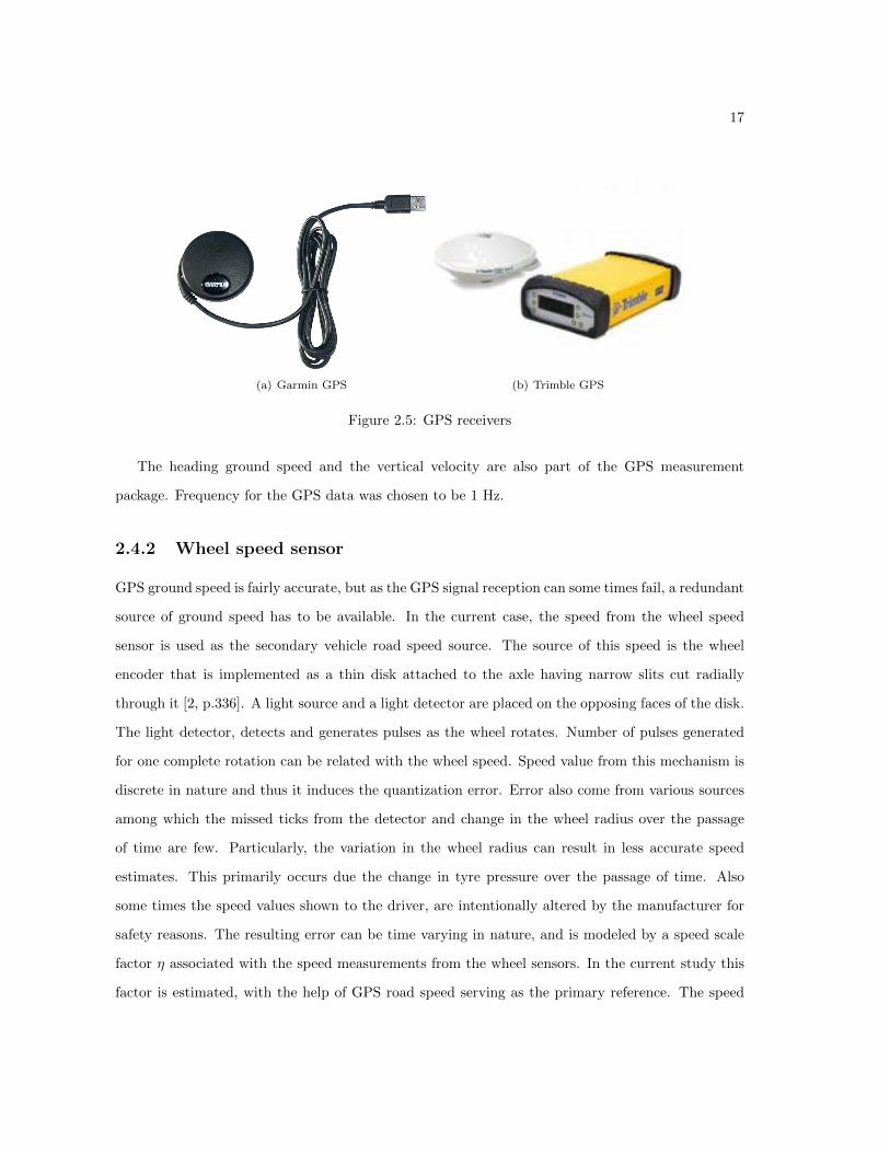
A low cost Garmin GPS was used for taking the measurements with the position error CEP
(Circular Error Probability)of five meter. It was replaced by a highly accurate RTK (Real Time
Kinematic) enabled Trimble GPS, model SPS 852. The RTK GPS receives a correction signal send
by a local base station and provides the position estimates with CEP in range of 10 cm.
17
(a) Garmin GPS (b) Trimble GPS
Figure 2.5: GPS receivers
The heading ground speed and the vertical velocity are also part of the GPS measurement
package. Frequency for the GPS data was chosen to be 1 Hz.
2.4.2 Wheel speed sensor
GPS ground speed is fairly accurate, but as the GPS signal reception can some times fail, a redundant
source of ground speed has to be available. In the current case, the speed from the wheel speed
sensor is used as the secondary vehicle road speed source. The source of this speed is the wheel
encoder that is implemented as a thin disk attached to the axle having narrow slits cut radially
through it [2, p.336]. A light source and a light detector are placed on the opposing faces of the disk.
The light detector, detects and generates pulses as the wheel rotates. Number of pulses generated
for one complete rotation can be related with the wheel speed. Speed value from this mechanism is
discrete in nature and thus it induces the quantization error. Error also come from various sources
among which the missed ticks from the detector and change in the wheel radius over the passage
of time are few. Particularly, the variation in the wheel radius can result in less accurate speed
estimates. This primarily occurs due the change in tyre pressure over the passage of time. Also
some times the speed values shown to the driver, are intentionally altered by the manufacturer for
safety reasons. The resulting error can be time varying in nature, and is modeled by a speed scale
factor η associated with the speed measurements from the wheel sensors. In the current study this
factor is estimated, with the help of GPS road speed serving as the primary reference. The speed

18
measurement, therefore can be written as
Vwss = (1 + η)V + vwss. (2.30)
where Vwss is the measured speed from the speed sensors, V is the actual speed and η is the
speed scale factor. vwss is the measurement noise in the speed signal. A non-zero value of η means
represents the deviation of the WSS measurement from the true value.
2.4.3 Acceleration sensors
Two types of acceleration signals are available from the embedded sensors in the truck. One is the
longitudinal acceleration ax. This signal is obtained by differentiating the vehicle speed got from
the tachograph. Apart from the longitudinal acceleration, the lateral acceleration signal ay is also
measured. It source is an accelerometer present in the truck that directly measures the body y-axis
acceleration. This signal also contains an inherent bias, which may be time varying in nature. It
represents the degree of imprecision in the instrument manufacturing. The acceleration measurement
model, is therefore given by the equations 2.31 and 2.32,
ax = ax + valong (2.31)
ay = ay + bay + valat. (2.32)
where ax and ay are the measured accelerations, ax and ay are the actual acceleration values, bay
is the bias value associated with the lateral accelerations, and valong and valat are the noise signals.
As mentioned above, the longitudinal acceleration is not obtained by the accelerometer, therefore
there is no bias signal associated with it.
2.4.4 Gyro and steering sensor
Scania test truck contains a gyro scope that measures the rate of change of the yaw-angle also called
the yaw-rate. Again the gyro scope is modeled as the accelerometer i.e.
ω = ω + bω + vω (2.33)
19
where ω is the measured yaw-rate, ω is the actual yaw-rate , bω is the bias signal for the yaw-rate,
and vω is the noise signal.
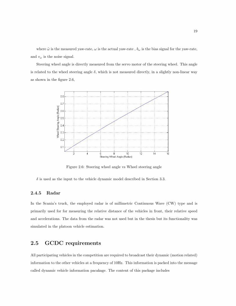
Steering wheel angle is directly measured from the servo motor of the steering wheel. This angle
is related to the wheel steering angle δ, which is not measured directly, in a slightly non-linear way
as shown in the figure 2.6,
Figure 2.6: Steering wheel angle vs Wheel steering angle
δ is used as the input to the vehicle dynamic model described in Section 3.3.
2.4.5 Radar
In the Scania’s truck, the employed radar is of millimetric Continuous Wave (CW) type and is
primarily used for for measuring the relative distance of the vehicles in front, their relative speed
and accelerations. The data from the radar was not used but in the thesis but its functionality was
simulated in the platoon vehicle estimation.
2.5 GCDC requirements
All participating vehicles in the competition are required to broadcast their dynamic (motion related)
information to the other vehicles at a frequency of 10Hz. This information is packed into the message
called dynamic vehicle information pacakage. The content of this package includes
20
1. Vehicle Position
2. Vehicle Position Timestamps
3. Vehicle Position Accuracy
4. Vehicle Speed
5. Vehicle Acceleration
6. Vehicle Heading
7. Vehicle Yaw-Rate
In addition to this information, vehicle are also required to transmit the so called static vehicle
information message. The contents of this message includes
1. Vehicle Length
2. Vehicle Width
GCDC committee has also mentioned the accuracy requirements for the dynamic states that
each competing vehicle has to fulfill. These are listed below
Position accuracy It is impractical to define the absolute accuracy for the GPS receiver position
estimates. The reason is that these estimates are themselves dependant on multiple factors like the
time of the day, number of visible satellites, atmospheric conditions, radio channel behavior and
receiver antenna placement etc. GCDC requirement for the position accuracy εp is given by
εp ≤ 1m (2.34)
Speed accuracy Only longitudinal speed estimates are required to be transmitted. The criteria
for the speed accuracy is εs is given by
εs ≤ 0.5ms−1 (2.35)

21
Acceleration accuracy Here again the longitudinal acceleration is meant. The criteria for the
acceleration accuracy εa is given by
εa ≤ 0.2ms−2 (2.36)

Chapter 3
Single Vehicle Estimation
The basic purpose of the current thesis is to device some strategy to estimate the dynamic states of
the vehicle and of platoon. This chapter deals with the state estimation of a single vehicle i.e. the
test vehicle, which is also referred as the Ego vehicle by the GCDC committee. In the Section 3.1,
a brief overview of the vehicular states that are to be estimated is given. This forms the basis of
the more detailed analysis presented in the subsequent sections of the chapter. A vehicle is required
to be modeled mathematically , such that the model can be used together with the sensors data in
the estimation process. Next part of this chapter covers the details of dynamic modeling of the ego
vehicle. Two types of models have been analyzed in course of current thesis work. These include a
kinematic model, which does not make any direct reference to the forces acting on the vehicle, and
a dynamic model referred in the text as the bicycle model which takes into account the forces acting
on the vehicles body. Section 3.2 describes the details of the kinematic model for the ego vehicle.
Section 3.3 deals with the description of the Bicycle model of the vehicle. Covariance matrices are
discussed in the Section 3.4.
3.1 States of a vehicle
In the scope of this thesis, only those vehicular states that are related to the motion and controlling
of the vehicle have been studied and implemented. Such a model is also referred as the six degrees
of freedom (6-DoF) model. This model assumes that the vehicle can translate along three principle
orthogonal axis and as well as rotate about these them, hence making the degree of motion freedom,
22
23
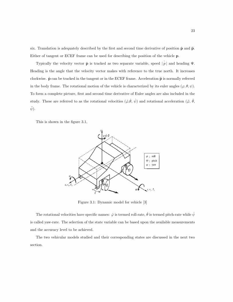
six. Translation is adequately described by the first and second time derivative of position p and p.
Either of tangent or ECEF frame can be used for describing the position of the vehicle p.
Typically the velocity vector p is tracked as two separate variable, speed ˙| p | and heading Ψ.
Heading is the angle that the velocity vector makes with reference to the true north. It increases
clockwise. p can be tracked in the tangent or in the ECEF frame. Acceleration p is normally referred
in the body frame. The rotational motion of the vehicle is characterized by its euler angles (ϕ, θ, ψ).
To form a complete picture, first and second time derivative of Euler angles are also included in the
study. These are referred to as the rotational velocities (ϕ,θ, ψ) and rotational acceleration (ϕ, θ,
ψ).
This is shown in the figure 3.1,
Figure 3.1: Dynamic model for vehicle [3]
The rotational velocities have specific names: ϕ is termed roll-rate, θ is termed pitch-rate while ψ
is called yaw-rate. The selection of the state variable can be based upon the available measurements
and the accuracy level to be achieved.
The two vehicular models studied and their corresponding states are discussed in the next two
section.

24
3.2 Kinematic model
Kinematic is the branch of mechanics that deals with the motion of the objects with out explicitly
mentioning the causes i.e. forces behind. A kinematic model is a mathematical description of an
object in motion e.g a vehicle, that can be used to describe its motion parameters like position,
velocity, acceleration, heading etc. at any given moment of time. A kinematic model can be the
most convenient representation of a vehicle as it does not requires the intricate knowledge of the
vehicle’s dynamics which in some cases are quite difficult to model. Such a model provides a nice
trade-off between the complexity and the accuracy.
As discussed in the previous section, any ,moving object can be thought to exhibit 6 DoF while in
motion. In practice for an autonomous or semi-autonomous vehicle, the expressable or controllable
degree of freedom is usually less than six. A vehicle is limited in the way it can move. In other
words, while a position and orientation may be achievable, a vehicle’s current configuration often
limits its ability to reach the posture without careful maneuvering or judicious use of its local degrees
of freedom. Therefore a vehicle can be thought of as a non-holonomic system. In a non-holonomic
system, the controllable degrees of freedom are in general less than the total degrees of freedom. A
car could translate in all three orthogonal axes. Although in almost all the cases, a car does not slide
in the plane perpendicular to the forward direction or jump off the ground [7]. Also it is assumed
that the vehicle cannot side-slip. Suppose Vb represents the vehicle longitudinal velocity. Then in
the body frame centered at the center of gravity (CoG) of the vehicle, it will have components Vbx,
Vby and Vbz. Non-holonomic constraint implies that
Vb =
vbxvbyvbz
=
vx0
0
(3.1)
Where vby = 0 means that the vehicle cannot slip along the side and vbz = 0 implies that vehicle
cannot suddenly jump off ground.
Further simplifications can be made in the model based on the measurements sensors available
and the nature of the terrain followed by the vehicle. If it is assumed that the vehicle will be mostly
traveling on a flat stretch of road, thus either of the roll-rate and pitch rate or both can neglected.

25
In the current project there is no source available for measuring roll-rate. Therefore this assumption
of zero roll rate ϕ is well motivated. As for the vehicle pitch, this may or may not be ignored. The
effect of the vehicle roll can be compensated by using suitable value for the error covariances inside
the Kalman filter. There is no sensor directly measuring the pitch rate, but an indirect observation
can be derived using the GPS vertical velocity vgpsd and the GPS ground velocity vgpsg such that
sinθ =vgpsd
vgpsg(3.2)
cosθ =
√1− (
vgpsd
vgpsg)2. (3.3)
Some of the vehicle test maneuvers are performed on the Scania’s main test track, which pitch’s
up at certain segments. This is shown in the figure 3.2
Figure 3.2: Scania’s test track
Hence it seems to be a judicious choice, not to ignore the vehicle’s pitch motion.
3.2.1 Process model
The GCDC dynamic vehicle information message contents as described in the Section 2.5, form the
basis for the selection of state vector in any of the studied model. Then there are some additional
states that are defined to improve the accuracy of the basic states.
Position p of the vehicle can be described either in ECEF or in the local tangent frame. Local

26
tangent frame representation is a preferred choice as it gives the position details with respect to a
locally defined origin, which results in easy tracking. It will have components [pe, pn, pu], which are
related to the components of the velocity in the ENU frame as given in the equation 3.4,
pe
pn
pu
=
Ve
Vn
Vu
. (3.4)
The velocity vector of the vehicle in the ENU frame is related to the longitudinal and lateral
velocity in the body frame by the transpose of (2.2). This requires the knowledge of the euler angles
(ϕ, θ, ψ). Roll angle ϕ is ignored in the current work. Hence the transformation matrix Rgb , for the
current case in the light of the assumption made above, is given by equation 3.5,
Rgb =
sinψ cosθ cosψ sinψ sinθ
cosψ cosθ −sinψ cosψ sinθ
−sinθ 0 cosθ
. (3.5)
Here sin θ and cos θ are given by (3.2). Using the above transformation matrix, the velocity in
the local tangent frame is given by (2.1). Therefore
Ve
Vn
Vu
=
vxsinψ cosθ
vxcosψ cosθ
−vxsinθ
(3.6)
Using equations (3.2) and (3.4), the velocity vector in ENU frame can be related to the derivative
of position vector. This is given by the equation (3.7),

27
pe
pn
pu
=
vxsinψ cosθ
vxcosψ cosθ
−vxsinθ
=
vxsinψ
√1−
v2dv2x
vxcosψ
√1−
v2dv2x
− vd
. (3.7)
Only the longitudinal acceleration i.e. the x-component of the body acceleration is taken into
account in this model.
ab =
abx
aby
abz
=
ax
0
0
. (3.8)
Velocity and acceleration are related by the equation (3.9)
vx = ax. (3.9)
Here ω is the yaw-rate of the vehicle.It is related to Vehicle yaw or the heading angle ψ as
ψ = ω. (3.10)
As discussed earlier, speed from the wheel speed sensor together with the speed from the GPS
are used as observations. This wheel speed can be slightly in-accurate primarily due to the change
in the tyre pressure over the course of time as well as the due the inherent limitation of the speed
estimation mechanism built in the system, as described in the section 2.4.2. In contrast the speed
from the GPS is accurate with in 2 to 5 cm when the vehicle is moving considerably fast. Hence the
GPS speed or serves as a reference speed for the Model and the wheel speed is adjusted accordingly.
This is modeled by introducing a speed adjustment scale factor η which is also one of the states of
the state vector.

28
The remainder states include acceleration ax , yaw-rate ω, vertical velocity vd, speed scale factor
η, and yaw gyro bias bω, all of which are modeled as random walk. Over all, the state vector X for
the kinematic model consist of 10 states, which are shown in the equation (3.11),
X = [pe pn pu vx vd ax ψ ω η bω] t. (3.11)
Continuous time model equations
Kinematic Model in continues time is a non-linear model of form Xt = f(Xt), and can be written
by combining the state-rate equations given above. This is shown in the equation set (3.12),
pe = vxsinψ
√1−
v2dv2x
pn = vxcosψ
√1−
v2dv2x
pu = − vd
vx = ax
vd = 0
ax = 0
ψ = ω
ω = 0
η = 0
bω = 0
(3.12)
Discrete time model equations
Solution to the above continuous time differential equations can be found for time t > t0, where
t0 is the initial time instant. Here the moments of interest at which the filter periodically updates
are t = n dt, where dt is the update rate of the filter. Therefore the continuous time model given

29
above which has to be discretized for the implementation. Derivative X is replaced according to the
equation (3.14)
X =Xk −Xk−1
dt(3.13)
In discrete time the kinematic model will be of form Xk+1 = f(Xk)+nk, where nk is the process
noise vector that drives the process. Discrete model is then given by equation (3.14)
pe,k = pe,k−1 +
(vx,k−1sinψk−1
√1−
v2d,k−1
v2x,k−1
)dt + ne
pn,k = pn,k−1 +
(vx,k−1cosψk−1
√1−
v2dk−1
v2x,k−1
)dt + nn
pu,k = pu,k−1 − vd,k−1 dt + nu
vx,k = vx,k−1 + ax,k−1 dt + nvx
vd,k = vd,k−1 + nvd
ax,k = ax,k−1 + nax
ψk = ψk − 1 + ωk−1 dt + nψ
ωk = ωk−1 + nω
ηk = ηk−1 + nη
bω,k = bω,k−1 + nω
(3.14)
Here nk, the process noise vector, given by nk = [ne nn nu nvx nvd nax nψ nω nη nω] t.
It is assumed that the vector nk is uncorrelated, zero mean and gaussian with a co-variance
matrix Qk. Also, Qk is assumed to be diagonal matrix.
A point of interest is that even though position, speed and heading in the continuous time model
do not include process noises, noise is included in the discrete model. These terms are included
in the model due to the fact that there might be additional sources of error that have not been

30
modeled. One example is the assumption used that the roll rate of the vehicle is zero. As this is not
correct, corresponding error terms are added to the position state equations. Also there is normally
a wheel slip that has not been modeled here.
Since this is a non-linear model, EKF will be applied to this situation as described in the section
2.3.2. State propagation is carried by the equations (3.14). The covariance matrix is propagated
through equation (2.22) which requires the state transition matrix Fk. This is done by linearizing
the model around the previous state estimate, Xk−1|k−1. The matrix Fk, which is the Jacobian of
the function f(Xk) + nk w.r.t to Xk is given by equation (3.16)
F[i,j] =∂f(Xi)
∂Xj
∣∣∣∣Xk−1|k−1
(3.15)
Fk =
1 0 0 F1,4 F1,5 0 F1,7 0 0 0
0 1 0 F2,4 F2,5 0 F2,7 0 0 0
0 0 1 0 −dt 0 0 0 0 0
0 0 0 1 0 dt 0 0 0 0
0 0 0 0 1 0 0 0 0 0
0 0 0 0 0 1 0 0 0 0
0 0 0 0 0 0 1 dt 0 0
0 0 0 0 0 0 0 1 0 0
0 0 0 0 0 0 0 0 1 0
0 0 0 0 0 0 0 0 0 1
(3.16)
The variables Fij used in the above matrix are given in the table 3.1, where discrete time subscript
k has been dropped for convenience.

31
F1,4 = sinψ
(vx√
v2x − v2
d
)dt
F1,5 = sinψ
(−vd√v2x − v2
d
)dt
F1,7 = cosψ(√
v2x − v2
d
)dt
F2,4 = cosψ
(vx√
v2x − v2
d
)dt
F2,5 = cosψ
(−vd√v2x − v2
d
)dt
F2,7 = − sinψ(√
v2x − v2
d
)dt
Table 3.1: Definition of the notations used in the F matrix
3.2.2 Measurement model
Measurement model includes data from the GPS and CAN bus, contained in the CAN messages as
described in the section 2.4. As the message frequency is different for the messages, they have to be
aligned chronologically before data is extracted from them and subsequently used.
The measurement vector for the Kinematic Model is given by equation (3.17),
Yk = [pgpse,k , pgpsn,k , p
gpsu,k , v
canx,k , v
gpsG,k, v
gpsd,k , a
canx,k , ψ
gpsk , ωcank ] t. (3.17)
The above can be related to the output equations of the sensors to form the measurement model,
which turns out to be non-linear in nature. Hence it is of form Yk = h(Xk) + ek, where ek is the
measurement noise vector, in which individual sensors own a part.
The discrete time equations are given by the equation set (3.18),

32
pgpse = pe + ee
pgpsn = pn + en
pgpsu = pu + eu
vcanx,k = (1 + ηk) vx,k + ev,can
vgpsG,k = vx,k + ev,gps
vgpsd,k = vd,k + evd
acanx,k = ax,k + eax
ψgpsk = ψk + eψ
ωcank = ωk + bgyro,k + eω
(3.18)
The measurement noise vector ek is given by ek = [ee, en, eu, ev,can, ev,gps, evd, eax, eψ, eω] t
.
It is assumed that, as in the case of the process noise matrix, that the vector ek is uncorrelated,
zero mean gaussian vector with the co-variance matrix Rk. Hence, Rk is assumed to be a diagonal
matrix.
Linearization of the model is done around the current state estimate, Xk|k−1. This results in the
observation matrix Hk. The matrix Hk, which is the Jacobian of the function h(Xk) + vk w.r.t to
Xk, is given by
H[i,j] =∂h(Xi)
∂Xj
∣∣∣∣Xk|k−1
, (3.19)

33
Hk =
1 0 0 0 0 0 0 0 0 0
0 1 0 0 0 0 0 0 0 0
0 0 1 0 0 0 0 0 0 0
0 0 0 (1 + ηk) 0 0 0 0 vx,k 0
0 0 0 1 0 0 0 0 0 0
0 0 0 0 1 0 0 0 0 0
0 0 0 0 0 1 0 0 0 0
0 0 0 0 0 0 1 0 0 0
0 0 0 1 0 0 0 1 0 0
. (3.20)

34
3.3 Bicycle model
Kinematic model is provides a convenient way of modeling a vehicle as it does not requires the
knowledge of the actual dynamics involved. As described in the previous section, a zero lateral
velocity vy = 0, assumption was made. This in turn implies zero lateral force on the vehicle.
Normally for the straight stretch of road this assumption is quite reasonable, but during constant
cornering or turning of vehicle this may not be true. Even during sudden turns there is a significant
lateral acceleration of the vehicle. Hence, the vehicle’s velocity vector is no longer along the vehicle’s
longitudinal axis but slips in the direction of the turn. This generates the so called side slip angle
β of the vehicle. The β is defined as the angle of the velocity vector from the longitudinal axis of
the vehicle body. That is to say, the side slip angle is the difference of the GPS heading ψgps and
the yaw-angle or the angle of the vehicle’s velocity vector ψ . Neglecting the β, can have significant
influence on the vehicle’s positioning during certain maneuvers. Hence, a study of the vehicle’s
lateral dynamics becomes important in order to accurately model the vehicle’s behavior.
One of the popular model used in the study of lateral dynamics of the vehicle is the Bicycle Model.
The bicycle model is a two wheel model which assumes that the dominant effect on vehicle steering
is tire slip caused by angular acceleration. This can also be interpreted as while turning, the forces
acting along longitudinal direction of the vehicle as well as the wheel angular acceleration are as-
sumed to be zero, i.e vx = 0 and ωwheel = 0, whereas a net lateral force is assumed to be acting
upon the vehicle. This results in a lateral velocity. Assuming non-zero lateral velocity, the vehicle
velocity vector in the body frame is given by equation (3.21),
Vb =
vbx
vby
vbz
=
vx
vy
0
. (3.21)
Additionally, the lateral and longitudinal weight shifts defined as the shift of the weight from one
side of the vehicle to the other under angular accelerations (mostly due to cornering) are assumed
to be negligible. A front wheel driven vehicle is assumed in the following analysis. This is illustrated
in figure 3.3.

35
Figure 3.3: Bicycle model for vehicle [4]
In figure 3.3, β is the side slip angle at the CoG of vehicle, and ψ is the vehicle yaw-angle. δ
is the front wheel steering angle. ν represents the angle of vehicle’s velocity vector, which is it’s
heading. Vehicle velocity V is also the body frame velocity vb. All of these variables are referenced
at the Center of Gravity (CoG)of the vehicle. a is the distance of the CoG from the front wheel and
b is the angle of the back wheel from the CoG. The side slip at the tyres is not same as at the CoG
due to the difference in the velocities at the individual tyres. Therefore the side slip at the front
wheel is given by αF and at rear wheel is given by αR. FyF is the lateral force acting on the front
wheel whereas FyR is rear wheel lateral force.
3.3.1 Process model
The process model, in this case, is described in three parts. In the first part the model without
the navigation equations is developed. This only contains states necessary to estimate the lateral
dynamics of the vehicle, that is to say purely bicycle model. It is done in order to clearly explain the

36
mathematical structure of the bicycle model. As it will be seen that the bicycle model, needs the
speed estimates in order to estimate the lateral dynamics of the vehicle. In order to do so, a speed
estimation model is presented in the second part. Finally, in the third part, a navigation model is
presented.
Lateral dynamics estimation sub model
Starting with the Newton second law of motion, the net forces acting along the body can be written.
m ay = FyF + FyR (3.22)
m ax = 0, (3.23)
where m is the mass of the vehicle and ay is the inertial acceleration at the CoG along the vehicle
body y-axis. There are two contributing terms to ay: y which represents the sidewards acceleration
of the vehicle, and Vx ψ which represents the centripetal acceleration during the turning maneuver
of vehicle [8].
ay = y + vx ψ (3.24)
Equation (3.22), can be written by using the equation (3.24) as
m (y + vx ψ) = FyF + FyR (3.25)
Also, the balancing the moment about the z-axis, the yaw-dynamic equations can be written as
Iz ψ = aFyF − b FyR (3.26)
where Iz is the vehicle moment of inertia about the z-axis.
The next step is to model the lateral forces acting on the tyres. The most commonly used is
the linear tyre model that assumes that the relationship between the Lateral force and the tyre slip
angle is linear in a certain region as shown in the figure 3.4
Hence the equations for the lateral force on the tyres are given as

37
Figure 3.4: Lateral force vs the tyre slip angle [5]
FyF = −2 αF CF (3.27)
FyR = −2 αR CR (3.28)
where CF and CR are the cornering squiffiness of the tyres mentioned in the 3.4 as Cα which is
the slope of the graph. These are predetermined constants. The tyre slip angles αF and αR depend
on multiple variables, including the side slip angle β, vehicle yaw-rate ψ, vehicle dimensions etc. [8].
They are given as
αF = β + a ψvx− δ (3.29)
αR = β − b ψvx
(3.30)
Also as discussed above, the vehicle produces side-slip angle during cornering. The heading
measurement from the GPS, in that case, will be the sum of the yaw-angle and side slip
ψgps = β + ψ, (3.31)
where ψ is defined in the equation (3.10).
Hence, the side slip β, has to be estimated separately in order to get the correct yaw-angle of
the vehicle, by subtracting β from the GPS heading ν measurement.

38
The lateral acceleration and the yaw-rate bias signals are used as observations, as will be discussed
later in detail. These signals come from the accelerometer and the gyro embedded in the truck , and
it was mentioned in the Section 2.4 that time varying biases bay and bω are also associated with the
them. They are modeled as random walk given by
bay = 0
bω = 0
(3.32)
Hence it needs to be estimated, in order to get the correct value of lateral acceleration signal.
The state vector for the lateral dynamics model becomes
X(lat) = [β , ω , ψ , bay , bω , vy]t (3.33)
By combining the equations (3.29) and (3.27) and putting them in the equations (3.25) and
(3.26), together with equations (3.10) and (3.32), the state space equations for the lateral dynamics
model can be derived, as given in [9], [10] and [4]. This is shown in the equation set (3.34),
β
ω
ψ
bay
bω
vy
=
−CF−CR
mvx−a CF+b CR
mv2x− 1 0 0 0 0
−a CF+b CR
Iza2 CF+b2 CR
Izvx0 0 0 −a CF+b CR
Izvx
0 1 0 0 0 0
0 0 0 0 0 0
0 0 0 0 0 0
0 −vx + −a CF+b CR
mvx0 0 0 −CF−CR
mvx
β
ω
ψ
bay
bω
vy
+
CF
mvx
a CF
Iz
0
0
0
CF
m
δ(3.34)
.
In the above model, longitudinal velocity vx and the wheel steering angle δ appears as the control
input. Lateral velocity in this case is not directly related to lateral acceleration, but defined as a
function of terms of vx, ω and δ. Discretization of the above model is done according to (3.13).
Appropriate process noise vector nk is added to the discrete time model.

39
Speed estimation sub model
It is mentioned above that the longitudinal velocity or simply the vehicle’s speed appears as a control
input in the bicycle model equations. But as it was discussed in the Section 3.1, the speed has to
be corrected and the corresponding scale factor has to be estimated before using the signal in the
estimation process. In the current scenario, this has to be done before equations (3.34) are evaluated.
Therefore a speed estimation filter is employed. Vertical velocity is also part of the estimation.The
state vector for the speed estimation model becomes
X(spd) = [vx , vd , ax , η] t (3.35)
The continuous time state equations are described in the equation (3.36),
vx = ax
vd = 0
ax = 0
η = 0
(3.36)
In the above equations, vx is the speed or the longitudinal velocity, vd is the vertical speed, ax
is the longitudinal acceleration and η is the speed scale factor. Discretization of the above model is
done according to (3.13). Appropriate process noise vector nk is added to the discrete time model.
Navigation sub model
The navigation model describes the motion equations for the vehicle. The data from the lateral
dynamic estimation filter and the speed estimation filter serve as an input. The state vector X for
the navigation model consist of 3 states, which are given by the equation (3.37),
X(nav) = [pe pn pu ] t. (3.37)
It was mentioned that the pitch angle is approximated by the ratio of the vehicle’s vertical velocity

40
and the horizontal velocity. There is one important fact to note; during the straight traveling of
the vehicle, the GPS ground speed vG and the longitudinal velocity vx are same. But during the
turning the vehicle can have a lateral component vy of velocity. This component can be significant,
depending on the turn rate. Therefore, vG is related to the two velocity components vx and vy by
the equation (3.38),
vx = vG cos β
vy = vG sin β(3.38)
and
vG =√v2x + v2y . (3.39)
Here, β is the side slip angle. As a result of the lateral component of the velocity, the expression
of the the sin and cos mentioned in the equation (3.2) are changed. The new expressions are given
by
sinθ =vd√
v2x + v2y
(3.40)
cosθ =
√1− (
v2dv2x + v2y
). (3.41)
Using equations (3.40) and (3.4), velocity vector in ENU frame can be related to the derivative
of position vector. This is given by the equation (3.42),
pe
pn
pu
=
vxsinψ cosθ + vy cosψ
vxcosψ cosθ − vy sinψ
−vxsinθ
=
vxsinψ
√1−
v2dv2x + v2y
+ vy cosψ
vxcosψ
√1−
v2dv2x + v2y
− vy sinψ
−vx vd√v2x + v2y
.(3.42)
41
Here vx, vy, vd and ψ appear as the control input . Discretization of the above model is done
according to (3.13). Appropriate process noise vector nk is added to the discrete time model.

42
3.3.2 Measurement model
In the following sections the measurement models associated with the three process models are
described.
Lateral dynamics estimation sub model
The measurement vector for the Lateral Dynamics Model is given by the equation (3.43)
Y(lat)k = [ψgpsk , ωcank acany,k , ]
t (3.43)
The vector Y(lat)k is related to the vector X
(lat)k as described by the equation set (3.44),
ψgpsk = ψk + eψ
ωcank = ωk + eω
acany,k =−a CF − b CR
mvxωk +
−CF − CRmvx
vy,k + bay +CFm
δk + eay
(3.44)
The observation equation for the lateral velocity is described in [11]. The measurement noise
vector e(lat) is given by e(lat) = [eψ, eω, eay]t . The observation model also includes δ as the
control input. The observation matrix in this case is given by equation set (3.45),
H(lat) =
0 0 1 0 0 0
0 1 0 0 0 0
0 −a CF−b CR
mvx0 1 0 −CF−CR
mvx
(3.45)
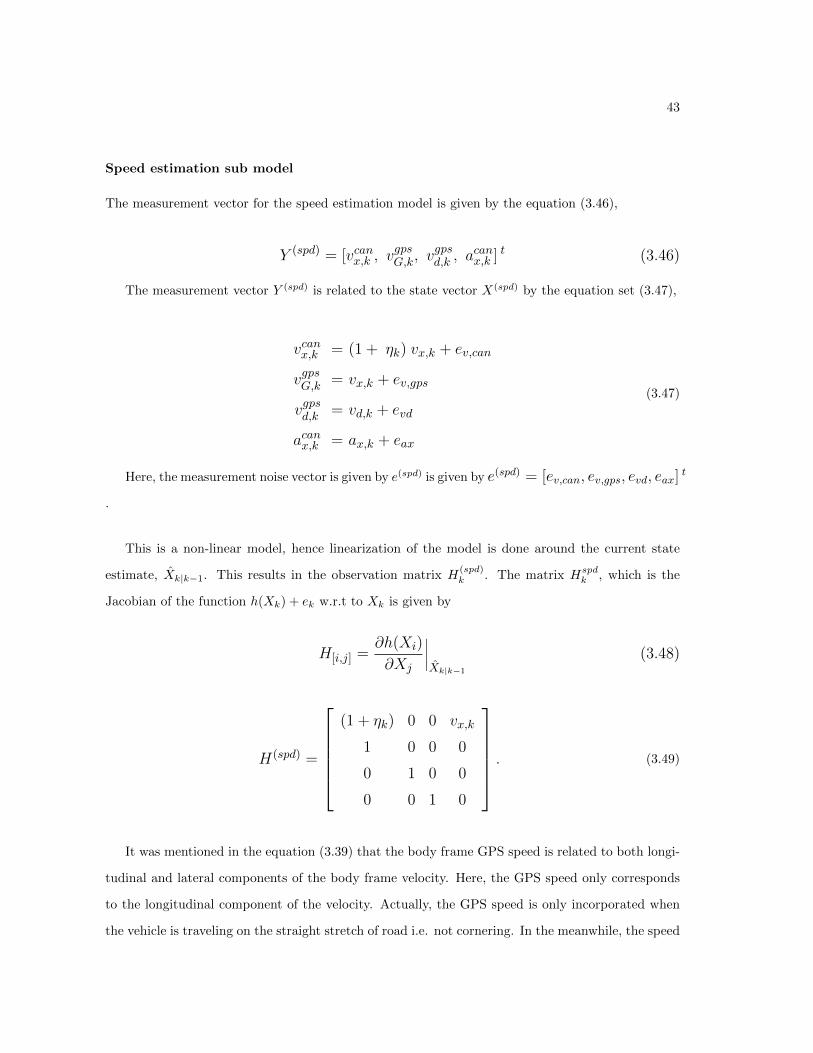
43
Speed estimation sub model
The measurement vector for the speed estimation model is given by the equation (3.46),
Y (spd) = [vcanx,k , vgpsG,k, v
gpsd,k , a
canx,k ] t (3.46)
The measurement vector Y (spd) is related to the state vector X(spd) by the equation set (3.47),
vcanx,k = (1 + ηk) vx,k + ev,can
vgpsG,k = vx,k + ev,gps
vgpsd,k = vd,k + evd
acanx,k = ax,k + eax
(3.47)
Here, the measurement noise vector is given by e(spd) is given by e(spd) = [ev,can, ev,gps, evd, eax]t
.
This is a non-linear model, hence linearization of the model is done around the current state
estimate, Xk|k−1. This results in the observation matrix H(spd)k . The matrix Hspd
k , which is the
Jacobian of the function h(Xk) + ek w.r.t to Xk is given by
H[i,j] =∂h(Xi)
∂Xj
∣∣∣∣Xk|k−1
(3.48)
H(spd) =
(1 + ηk) 0 0 vx,k
1 0 0 0
0 1 0 0
0 0 1 0
. (3.49)
It was mentioned in the equation (3.39) that the body frame GPS speed is related to both longi-
tudinal and lateral components of the body frame velocity. Here, the GPS speed only corresponds
to the longitudinal component of the velocity. Actually, the GPS speed is only incorporated when
the vehicle is traveling on the straight stretch of road i.e. not cornering. In the meanwhile, the speed

44
scale factor is estimated. When the vehicle start turning, the GPS speed measurement is ignored.
This is done by zeroing the second row of the H(spd)k matrix. The vehicle turning is determined
by setting a speed threshold on the yaw-rate of the vehicle.
Navigation sub model
The measurement vector for the process model is given by
Y(nav)k = [pgpse,k , p
gpsn,k , p
gpsu,k ] t (3.50)
The measurement vector Y(nav)k is related to the state vector X
(spd)k by the equation set (3.51),
pgpse = pe + ee
pgpsn = pn + en
pgpsu = pu + eu
(3.51)
Measurement vector is generated by transforming the GPS geodetic frame data (λ, φ, h) to the
tangent frame variables pe, pn, pu by equations (2.6) and (2.5). The measurement noise vector ek is
given by ek = [ee, en, eu]t .
The observation matrix in this case is given by,
H(nav) =
1 0 0
0 1 0
0 0 1
. (3.52)

45
3.3.3 Implementation
The bicycle model is therefore implemented as a cascade of three sub-filters. The first is the speed
estimation filter that feeds its estimates to the lateral dynamics model. Finally the navigation filter
is run based on the inputs from the former two filters. This is shown in the figure 3.5,
Figure 3.5: Bicycle model implementation
The speed estimation filter is an EKF while the lateral dynamics estimation filter and the navi-
gation filters are KFs.
3.4 Covariance matrices
Various process noise vectors, nk and measurement noise vectors, ek were mentioned throughout
the description of the Kinematic and Bicycle models. These noises are added to cater for the
uncertainties, that may be present due to non-modeled elements in the process model, and the
physical sensor noises in case of the measurement model. These noise vectors are assumed to
be normally distributed with zero mean and co-variance matrices Qk and Rk for the process and
measurement noises respectively. Dimensions of Qk are m × m and of Rk are n × n, where m is
the length of state vector and n is the length of the observation vector. Also, noise vectors are
approximated to be individually and mutually uncorrelated. This means that both of these matrices
will be diagonal matrices containing mean PSDs (Power Spectral Densities). This further highlights
the fact, that the state errors are mutually uncorrelated. Also the mutual correlation between the
two noise vectors, nk and ek is assumed to be zero i.e. a null matrix.

46
For the Kinematic model, a noise term is associated with individual state in the process model,
e.g. in the case of the position variables, this represents the lack of sophistication. This follows the
fact that the roll-rate of the vehicle is ignored and the pitch rate is not directly incorporated in the
model. While Rk can be ,made up by using the sensors error provided in the data sheets, the choice
of values of Qk is done more heuristically. Also a note worthy point is that, the relative values of the
two noise vectors, not the absolute values is what actually matters. A high value of Qk will result
in more uncertainty in the states and will lead to noisy estimates. In case of position estimates, this
will lead the filter to follow the GPS more closely. A high value of Rk mean that measurements have
high noise levels.
While the values for Qk are chosen to optimize the performance of the filter, the measurement
noise matrix Rk is filled with the PSD of sensors noises. E.g. position data accuracy heavily depends
upon the number of tracked satellites, atmospheric conditions, time of the day etc. It is defined in
terms of CEP (Circular Error Probability). CEP is defined as the radius of a circle centered on the
true value that contains 50 percent of the actual GPS measurements. Variance for the horizontal
position is related to the CEP by the formula(1.2CEP )√
2
2
. The GPS receiver used during the data
collection had horizontal CEP of 5 m. While, for the vertical position, a CEP of 15m was noted.
Table 3.2 describes the standard deviation for all sensor noises.
Measurement Noise PSD 1σ Measurement Noise 1σ
Position (East) 4.2 m Velocity (Vertical, GPS) 5e-1 ms−1
Position (North) 4.2 m Acceleration (Longitudinal) 1e-1 ms−2
Position (Up) 13 m Acceleration (Longitudinal) 5e-2 ms−2
Velocity (Ground, CAN) 1e-2 ms−1 Yaw Angle 1e-3 rad
Velocity (Ground, GPS) 5e-2 ms−1 Yaw Rate 1e-1 rads−1
Table 3.2: Measurement noise co-variance matrix Rk
Also as mentioned in the section 2.3, the state error matrix P is propagated using the equation
(2.22). However a initial estimate of P is required to start with. Initial estimate P0|0 is critical to
choose. Different values lead different transient response of the filter.

Chapter 4
Platoon Estimation
In the GCDC competition scenario, vehicles are supposed to form the so called platoons, that refer
to a stack or group of moving vehicle interacting with each other. Each vehicle shares its dynamic
states with the other as described in the Section 2.5. This information, together with the data from
the sensors onboard, is used to control the ego vehicle. As the data from the other vehicles reaches
via radio, it can be corrupted or delayed. Hence there arises a requirement of processing the data it
is passed on to the vehicle controller. This chapter deals with the estimation technique that can be
used for the platoon vehicles. Two platoon models have been studied in the course of the thesis work.
The first in the separate estimation model while the second is a joint estimation model. Section 4.1
deals with the formal description of the states associated with the platoon vehicles. In the Section
4.2, the separate estimation model for the platoon vehicle is mentioned. Joint estimation model is
described in the Section 4.3.
4.1 States of the platoon vehicle
Platoon of vehicle consist of more than one vehicle interacting with each other, in which the vehicle
at the absolute front is termed as the leader of the platoon. Each vehicle tries to keep the coherence
in the platoon by controlling its speed i.e. maintaining a constant speed profile and if necessary,
acceleration or deceleration. The vehicle controller decides which action to perform based on the
data from the estimation module [12], which is the focus of this study. A typical platoon scenario is
depicted in the figure 4.1,
47

48
Figure 4.1: Vehicles forming a platoon [1]
The estimation module is responsible for the data provision to the controller regarding the states
of the platoon vehicles. These states are a set of parameters associated with each individual vehicle
in relation to the ego vehicle influencing its behavior. These are also termed here as the control
states which are mentioned below
Relative Distance The relative distance of platoon vehicle relative to the Ego vehicle along the
axis of motion. This is a signed variable, positive for the vehicles ahead and negative for the
ones at the back
Absolute Speed The absolute speed of the platoon vehicle.
Absolute Acceleration The absolute acceleration of the platoon vehicle
The motivation for choosing this set of control states for each vehicle, is the requirement from
the controller as mentioned in [12]. This information together with some other is to be sent to the
controller via CAN message.
Like in the case of the ego vehicle estimation, two types of models are studied for the platoon
vehicles. The first is a separate estimation model, that estimates the states of each vehicle individ-
ually. It’s working resembles that of a parallel filter bank. The second model is a joint estimation
model where the states of all platoon vehicles are a part of common state vector. Ego vehicle data
appears as control input to the model. Relative distance is one of the states in the model, so radar
information is incorporated directly in to the filter. These models are explained following sections.

49
4.2 Separate estimation model
This model estimates the states for each vehicle in the platoon individually. Platoon states estimation
is done in two parts. First the so called local states are estimated. This approach resembles the
Kinematic model for the ego vehicle mentioned in the Section 3.2, but the state vector has a fewer
number of states . Once done, the relative distance is then calculated using the estimated local
states. If the platoon vehicle whose estimation is being done, is the one directly in front, then the
radar information also used and is fused together with the control states estimates from the filter,
via Weighted Least Squares (WLS) method. Figure 4.2 describes the whole process,
Figure 4.2: Separate estimation model representation
4.2.1 Process model
The main source of data available for the platoon vehicle state estimation is the radio. The content
of the radio message as mentioned in section 2.5, are limited which in turn entails the use of a fewer

50
state model for the vehicle representation. This results in the use of a planar motion model i.e. a
2D motion model, which also ignores lateral component of velocity or the side slip. As details of the
kinematic model were mentioned in previous chapter, therefore it is not explained here.
The local state vector X for the kinematic model consist of 6 states, which are given by equation
(4.1),
X = [pie pin v
ix a
ix ψ
i ωi ] t. (4.1)
Here the superscript i indicates that state vector is for the ith vehicle of the platoon. The discrete
state space model for the local state vector is given in the equation set (4.2),
pie,k = pie,k−1 + vix,k−1 sinψik−1 dt + nie
pin,k = pin,k−1 + vix,k−1 cosψik−1 dt + nin
vix,k = vix,k−1 + aix,k−1 dt + nivx
aix,k = aix,k−1 + niax
ψik = ψik−1 + ωk−1 dt + niψ
ωik = ωik−1 + niω
(4.2)
Here nk, the process noise vector, given by nk = [nie nin n
ivx n
iax n
iψ niω] t.
Furthermore, it is assumed that the vector nk is uncorrelated, zero mean and gaussian with a
co-variance matrix Qk. Also, Qk is assumed to be diagonal matrix.
The matrix Fk, which is the Jacobian of the non-linear model is given in the equation set (4.3),

51
Fk =
1 0 F1,3 0 F1,5 0
0 1 F2,3 0 F2,5 0
0 0 1 dt 0 0
0 0 0 1 0 0
0 0 0 0 1 dt
0 0 0 0 0 1
. (4.3)
The variables Fij used in the above matrix are given by the table (4.1),
F1,3 = sinψi dtF1,5 = vix cosψi dtF2,3 = cosψi dtF2,5 = −vix sinψi dt
Table 4.1: Definition of the notations used in the F matrix
In the above discussion, discrete time subscript k has been dropped for convenience.
4.2.2 Measurement model
All the measurement comes from the radio. The observation vector Yk is given by the equation (4.4),
Yk = [pi,re,k, pi,rn,k, v
i,rx,k, a
i,rx,k, ψ
i,rk , ωi,rk ] t (4.4)
Superscript r indicates that the source of the data is the radio. The discrete time equations of
the model are given in the equation (4.5),

52
pi,re,k = pie + eie
pi,rn,k = pin + ein
vi,rx,k = vix,k + eivx
ai,rx,k = aix,k + eiax
ψi,rk = ψik + eiψ
ωi,rk = ωik + eiω
(4.5)
The measurement noise vector ek is given by ek = [eie, ein, e
ivx, e
iax, e
iψ, e
iω] t
.
It is assumed that, like in the case of the process noise matrix, that the vector ek is uncorrelated,
zero mean gaussian vector with the co-variance matrix Rk. Hence, Rk is assumed to be diagonal
matrix.
4.2.3 Relative distance calculation
Once the above states are estimated by the EKF, relative distance is then calculated for the ith
vehicle. This is illustrated in the figure 4.3,
Here diagonal distance refer to the length of the line connecting the geometric centers of two
vehicles, whereas the longitudinal distance is the distance between centers along the axis of motion
of the Ego vehicle as defined in the beginning of the chapter. Also the Line Bearing is defined as
the angle of the line connecting the two vehicles centers w.r.t. the velocity vector (i.e. the heading
of the ego vehicle.
This is done in four steps. First the diagonal distance ∆ddiag between the ith and the Ego vehicle
ε is calculated by the equation (4.6),
∆ddiag =√
(pεe − pie)2 + (pεn − pin)2 (4.6)
In the second step, the angle between the diagonal line w.r.t. the north, ζ is calculated as

53
Figure 4.3: Description of relative states
ζ = arctan 2{(pεn − pin), (pεe − pie)}mod 2π (4.7)
Here arctan 2 is the inverse tangent function that yields the angle in range [−π , +π] and mod
represents the modulus operator. Hence, the line bearing αLB in the radians is calculated as
αLB = min {|φ− ζ| , |2π − φ− ζ|} (4.8)
where φ is the heading of ego vehicle in radians. Then comes the relative distance ∆d which is
given by the equation (4.9),

54
∆d =
+ |∆ddiagcos(αLB)| − (Li+Lε)2 if αLB ≤ |π/2|
− |∆ddiagcos(αLB)| − (Li+Lε)2 if αLB > |π/2|
(4.9)
Here Li and Lε are the lengths of the ith platoon vehicle and Ego vehicle respectively.
4.2.4 Vehicle ahead
The Vehicle Ahead is defined as the vehicle that is immediately in front of the ego vehicle. It has
a critical importance in the control of ego vehicle. Therefore it deserves special treatment in the
estimation process. The idea here is that the accuracy and reliability of the information of the
vehicle ahead can be significantly improved by fusing its estimated data with the data from the
radar. Data from the radar used here consist of relative distance to the vehicle ahead, relative speed
to which ego vehicle’s speed can be added to get the absolute speed of the vehicle ahead and absolute
acceleration of vehicle ahead.
Let Xctrl be the vector of the control states of dimension 3× 1 containing the relative distance,
absolute speed and absolute acceleration estimates from the EKF, and Xrdr be the vector of dimen-
sion 3 × 1 containing the relative distance, absolute speed and absolute acceleration of the vehicle
ahead from the radar. These two vectors have covariances matrices Pctrl and Prdr respectively. They
can be fused together by using the formula given in [13, p. 29-30],
Xfus = (P−1ctrl + P−1
rdr)−1(P−1
ctrlXctrl + P−1rdrXrdr) (4.10)
where Xfus is the fused vector having covariance matrix (P−1ctrl + P−1rdr)−1.
4.3 Joint estimation model
In the previous section the model for single platoon vehicle estimation was discussed. It was men-
tioned above that the states for the vehicle in the platoon are the same as the state basic states
defined for the ego vehicle. Then by using those states the relative distance is calculated. Some
additional insight can be gathered by realizing that in the cooperative driving scenario, the vehicles

55
are interconnected. This refers to the fact that the disturbance caused by the vehicles at the start
of the platoon, propagates till the end. Then it is the responsibility of the controller to dampen out
the effect. This is normally termed as the string stability [14]. What is important here, is the fact
that the vehicles of a platoon can be thought to be connected to each other as masses are attached
in a spring damper system. This is shown in the figure 4.4,
Figure 4.4: Platoon vehicles acting like spring mass System [6]
The platoon of vehicles therefore can be studied in the same way as the spring-damper system
is analyzed. This can become a joint estimation problem where the vehicles states form together a
combined state vector.
4.3.1 Process model
For a platoon of N vehicles, it is assumed that the vehicles are joined together by spring of stiffness
k and damper of damping c, in series. Mass of the ith vehicle is denoted by mi. Let the position
and the velocity of the ith vehicle be denoted by the vectors ri = [pie , pin ]
tand the ri = [pie , p
in ]
t
respectively . Also, let Ff be the force exerted by the vehicle in front and Fr be the force exerted
by the rear vehicle on the ith vehicle. Then the two forces can be expressed using the expressions
similar to that of spring-damper system as

56
Ff = k (ri+1 − ri − d(i+1,i)s ) + c (ri+1 − ri)
Fr = k (ri − ri−1 − d(i,i−1)s ) + c (ri − ri−1)
(4.11)
In the above equations d(i+1,i)s is defined as the d
(i+1,i)s = d.
ri+1 − ri‖ri+1 − ri‖
, where d > 0 is the
minimum distance that should be maintained for platoon safety [6]. The force Ff for the lead vehicle
is zero while the force Fr is zero for the last vehicle of the platoon. The forces acting on the ith
vehicle can be expressed using the Newton’s second law as
mi ri = Ff − Fr (4.12)
Combining equations (4.11) and (4.12) one can get following set of equations for all platoon
vehicles
ri =
k
mi(r2 − r1 − d
(2,1)s ) +
c
mi(r2 − r1) if i = 1
k
mi(ri+1 − ri − d
(i+1,i)s ) − k
mi(ri − ri−1 − d
(i,i−1)s )
+c
mi(ri+1 − ri) −
c
mi(ri+1 − ri) if 2 ≤ i ≤ N
− k
mi(rN − rN−1 − d
(N,N−1)s ) − c
mi(rN − rN−1) if i = N
(4.13)
Lets call ri+1 − ri as ∆ri+1,i, the relative distance of vehicle i+1 w.r.t. vehicle i and ri+1 − ri
as ∆vi+1,i which is the relative velocity of the vehicle i+1 w.r.t. vehicle i. Then the above equations
can be written as
ri =
k
mi(∆r2,1 − d
(2,1)s ) +
c
mi(∆v2,1) if i = 1
k
mi(∆ri+1,i − d
(i+1,i)s ) − k
mi(∆ri,i−1 − d
(i,i−1)s )
+c
mi(∆vi+1,i) −
c
mi(∆vi+1,i) if 2 ≤ i ≤ N
− k
mi(∆rN,N−1 − d
(N,N−1)s ) − c
mi(∆vN,N−1) if i = N
(4.14)

57
The the d(i+1,i)s which now becomes d.
∆ri+1,i
‖∆ri+1,i‖can be written as
d(i+1,i)s =
d(i+1,i)s,e
d(i+1,i)s,n
=
d (pi+1
e − pie)√(pi+1e − pie)
2+ (pi+1
n − pin)2
d (pi+1n − pin)√
(pi+1e − pie)
2+ (pi+1
n − pin)2
=
d ∆p
(i+1,i)e√
(∆p(i+1,i)e )
2+ (∆p
(i+1,i)n )
2
d ∆p(i+1,i)n√
(∆p(i+1,i)e )
2+ (∆p
(i+1,i)n )
2
(4.15)
A state space model can be generated out of the above equations. The state vector Xplt will
comprise of two relative states namely the vector relative distance ∆ri+1,i , the vector relative
velocity ∆vi+1,i for each vehicle pair (i+1 , i) as well as the absolute velocity ri and absolute
acceleration a for each vehicle i . In scaler form, the state vector Xplt can be written as
Xplt =
∆p(i+1,i)e
∆p(i+1,i)n
∆v(i+1,i)e
∆v(i+1,i)n
v(i)e
v(i)n
a(i)
(4.16)
Here acceleration ai is modeled as random walk.
In the current thesis work, a three vehicle model was studied in which two vehicles were simulated
to be in front of the ego vehicle. As the estimation for the ego vehicle is done separately from the
platoon vehicles, its data does not become the part of the state vector. In other words the equation
for i = 1 is not the part of the model. The reason for choosing this number of vehicles was to
keep the complexity of the model low enough to be simulated. Also the mass of each vehicle mi
was considered to be same. Therefore, the platoon model for only three vehicle is presented here.
Implementational details of the model are covered in the Chapters 5 and 7. With ego vehicle as
the Vehicle no. 1 and using equations (4.14) and (4.15) the platoon system model for two vehicles
(except ego vehicle) becomes

58
∆p(2,1)
e = ∆v(2,1)e
∆p(2,1)
n = ∆v(2,1)n
∆v(2,1)
e = 0
∆v(2,1)
n = 0
v(2)e = K1 (∆p(3,2)e − ∆p(2,1)e + d(2,1)s,e − d(3,2)s,e ) + K2 (∆v3,2e − ∆v2,1e )
v(2)n = K1 (∆p(2,1)n − ∆p(2,1)n + d(2,1)s,n − d(3,2)s,n ) + K2 (∆v(3,2)n − ∆v(2,1)n )
a(2) = 0
∆p(3,2)
e = ∆v(3,2)e
∆p(3,2)
n = ∆v(3,2)n
∆v(3,2)
e = 0
∆v(3,2)
n = 0
v(3)e = −K1 (∆p(3,2)e − d(3,2)s,e ) − K2 ∆v(3,2)e
v(3)n = −K1 (∆p(3,2)n − d(3,2)s,n ) − K2 ∆v(3,2)n
a(3) = 0
(4.17)
where K1 isk
mand K2 is
c
m. Also Both of these are design parameters.
One thing to note is that, from the ego vehicle perspective, the relative distance ∆r3,2 and relative
velocity ∆v3,2 are not important. What is required by the ego vehicle is the relative position and
velocity of lead vehicle 3 w.r.t itself i.e. ∆r3,1 and ∆v3,1. Now assuming that the relative distance is
measured from the geometric center of the vehicles, it is obvious that ∆r3,2 = ∆r3,1 - ∆r2,1. This
further implies that ∆v3,2 = ∆v3,1 - ∆v2,1. Putting these values in the continuous time model
and discretizing those equation, the discrete time model can be generated, which is given by

59
∆p(2,1)e,k = ∆p
(2,1)e,k−1 + ∆v(2,1)e ∆t + ndp1
∆p(2,1)n,k = ∆p
(2,1)n,k−1 + ∆v2,1n ∆t + ndp2
∆v(2,1)e,k = ∆v
(2,1)e,k−1 + ndv1
∆v(2,1)n,k = ∆v
(2,1)n,k−1 + ndv2
v(2)e,k = v2e,k−1 + (K1 (∆p
(3,1)e,k−1 − 2∆p
(2,1)e,k−1 + d(2,1)s,e − d(3,2)s,e ) + K2 (∆v
(3,1)e,k−1 − 2∆v
(2,1)e,k−1)) ∆t + nv1
v(2)n,k = v2n,k−1 + (K1 (∆p
(3,1)n,k−1 − 2∆p
(2,1)n,k−1 + d(2,1)s,n − d(3,2)s,n ) + K2 (∆v
(3,1)n,k−1 − 2∆v
(2,1)n,k−1)) ∆t + nv2
a(2)k = a
(2)k−1 + na1
∆p(3,1)e,k = ∆p
(3,1)e,k−1 + ∆v(3,1)e ∆t + ndp3
∆p(3,1)n,k = ∆p
(3,1)n,k−1 + ∆v(3,1)n ∆t + ndp4
∆v(3,1)e,k = ∆v
(3,1)e,k−1 + ndv3
∆v(3,1)n,k = ∆v
(3,1)n,k−1 + ndv4
v(3)e,k = v3e,k−1 + (−K1 (∆p
(3,1)e,k−1 − p
(2,1)e,k−1 − d(3,2)s,e ) − K2 (∆v
(3,1)e,k−1 − ∆v
(2,1)e,k−1)) ∆t + nv3
v(3)n,k = v3n,k−1 + (−K1 (∆p
(3,1)n,k−1 − ∆p
(2,1)n,k−1 − d(3,2)s,n ) − K2 (∆v
(3,1)n,k−1 − ∆v
(2,1)n,k−1)) ∆t + nv4
a(3)k = a
(3)k−1 + na2
(4.18)
Here nk, the process noise vector is given by
nk = [ndp1 ndp2 ndv1 ndv2 nv1 nv2 na1 ndp3 ndp4 ndv3 ndv4 nv3 nv4 na2] t
In the above equations, the position vector r1 = [p1e , p1n ]
tand the velocity vector r1 = [v1e , v
1n ]
t
of the ego vehicle appears as the control input uk.
As the model is non-linear of form f(Xk , uk) therefore an Extended Kalman Filter (EKF) will
be applied to this situation as described in the section 2.3.2. The matrix Fk, which is the Jacobian
of the function f(Xk) +nk w.r.t to Xk,as defined in the equation (3.15) is given by the equation set
(4.19),

60
Fk =
1 0 1 0 0 0 0 0 0 0 0 0 0 0
0 1 0 1 0 0 0 0 0 0 0 0 0 0
0 0 1 0 0 0 0 0 0 0 0 0 0 0
0 0 0 1 0 0 0 0 0 0 0 0 0 0
F5,1 F5,2 F5,3 0 0 0 0 F5,8 F5,9 F5,10 0 0 0 0
F6,1 F6,2 0 F6,4 0 0 0 F6,8 F6,9 0 F6,11 0 0 0
0 0 0 0 0 0 1 0 0 0 0 0 0 0
0 0 0 0 0 0 0 1 0 1 0 0 0 0
0 0 0 0 0 0 0 0 1 0 1 0 0 0
0 0 0 0 0 0 0 0 0 1 0 0 0 0
0 0 0 0 0 0 0 0 0 0 1 0 0 0
F12,1 F12,2 F12,3 0 0 0 0 F12,8 F12,9 F5,10 0 0 0 0
F13,1 F13,2 0 F13,4 0 0 0 F13,8 F13,9 0 F13,11 0 0 0
0 0 0 0 0 0 0 0 0 0 0 0 0 1
(4.19)
The variables Fi,j used in the above matrix are given in the table 4.2. Note that the time
subscript has been dropped for convenience.
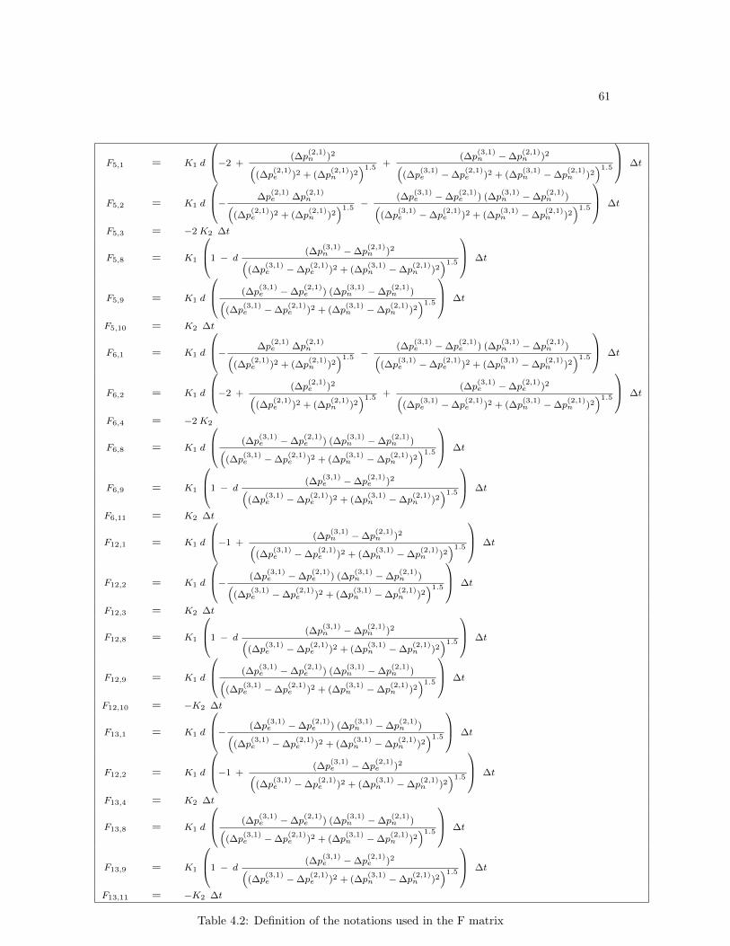
61
F5,1 = K1 d
−2 +(∆p
(2,1)n )2(
(∆p(2,1)e )2 + (∆p
(2,1)n )2
)1.5 +(∆p
(3,1)n − ∆p
(2,1)n )2(
(∆p(3,1)e − ∆p
(2,1)e )2 + (∆p
(3,1)n − ∆p
(2,1)n )2
)1.5 ∆t
F5,2 = K1 d
−∆p
(2,1)e ∆p
(2,1)n(
(∆p(2,1)e )2 + (∆p
(2,1)n )2
)1.5 −(∆p
(3,1)e − ∆p
(2,1)e ) (∆p
(3,1)n − ∆p
(2,1)n )(
(∆p(3,1)e − ∆p
(2,1)e )2 + (∆p
(3,1)n − ∆p
(2,1)n )2
)1.5 ∆t
F5,3 = −2 K2 ∆t
F5,8 = K1
1 − d(∆p
(3,1)n − ∆p
(2,1)n )2(
(∆p(3,1)e − ∆p
(2,1)e )2 + (∆p
(3,1)n − ∆p
(2,1)n )2
)1.5 ∆t
F5,9 = K1 d
(∆p(3,1)e − ∆p
(2,1)e ) (∆p
(3,1)n − ∆p
(2,1)n )(
(∆p(3,1)e − ∆p
(2,1)e )2 + (∆p
(3,1)n − ∆p
(2,1)n )2
)1.5 ∆t
F5,10 = K2 ∆t
F6,1 = K1 d
−∆p
(2,1)e ∆p
(2,1)n(
(∆p(2,1)e )2 + (∆p
(2,1)n )2
)1.5 −(∆p
(3,1)e − ∆p
(2,1)e ) (∆p
(3,1)n − ∆p
(2,1)n )(
(∆p(3,1)e − ∆p
(2,1)e )2 + (∆p
(3,1)n − ∆p
(2,1)n )2
)1.5 ∆t
F6,2 = K1 d
−2 +(∆p
(2,1)e )2(
(∆p(2,1)e )2 + (∆p
(2,1)n )2
)1.5 +(∆p
(3,1)e − ∆p
(2,1)e )2(
(∆p(3,1)e − ∆p
(2,1)e )2 + (∆p
(3,1)n − ∆p
(2,1)n )2
)1.5 ∆t
F6,4 = −2 K2
F6,8 = K1 d
(∆p(3,1)e − ∆p
(2,1)e ) (∆p
(3,1)n − ∆p
(2,1)n )(
(∆p(3,1)e − ∆p
(2,1)e )2 + (∆p
(3,1)n − ∆p
(2,1)n )2
)1.5 ∆t
F6,9 = K1
1 − d(∆p
(3,1)e − ∆p
(2,1)e )2(
(∆p(3,1)e − ∆p
(2,1)e )2 + (∆p
(3,1)n − ∆p
(2,1)n )2
)1.5 ∆t
F6,11 = K2 ∆t
F12,1 = K1 d
−1 +(∆p
(3,1)n − ∆p
(2,1)n )2(
(∆p(3,1)e − ∆p
(2,1)e )2 + (∆p
(3,1)n − ∆p
(2,1)n )2
)1.5 ∆t
F12,2 = K1 d
−(∆p
(3,1)e − ∆p
(2,1)e ) (∆p
(3,1)n − ∆p
(2,1)n )(
(∆p(3,1)e − ∆p
(2,1)e )2 + (∆p
(3,1)n − ∆p
(2,1)n )2
)1.5 ∆t
F12,3 = K2 ∆t
F12,8 = K1
1 − d(∆p
(3,1)n − ∆p
(2,1)n )2(
(∆p(3,1)e − ∆p
(2,1)e )2 + (∆p
(3,1)n − ∆p
(2,1)n )2
)1.5 ∆t
F12,9 = K1 d
(∆p(3,1)e − ∆p
(2,1)e ) (∆p
(3,1)n − ∆p
(2,1)n )(
(∆p(3,1)e − ∆p
(2,1)e )2 + (∆p
(3,1)n − ∆p
(2,1)n )2
)1.5 ∆t
F12,10 = −K2 ∆t
F13,1 = K1 d
−(∆p
(3,1)e − ∆p
(2,1)e ) (∆p
(3,1)n − ∆p
(2,1)n )(
(∆p(3,1)e − ∆p
(2,1)e )2 + (∆p
(3,1)n − ∆p
(2,1)n )2
)1.5 ∆t
F12,2 = K1 d
−1 +(∆p
(3,1)e − ∆p
(2,1)e )2(
(∆p(3,1)e − ∆p
(2,1)e )2 + (∆p
(3,1)n − ∆p
(2,1)n )2
)1.5 ∆t
F13,4 = K2 ∆t
F13,8 = K1 d
(∆p(3,1)e − ∆p
(2,1)e ) (∆p
(3,1)n − ∆p
(2,1)n )(
(∆p(3,1)e − ∆p
(2,1)e )2 + (∆p
(3,1)n − ∆p
(2,1)n )2
)1.5 ∆t
F13,9 = K1
1 − d(∆p
(3,1)e − ∆p
(2,1)e )2(
(∆p(3,1)e − ∆p
(2,1)e )2 + (∆p
(3,1)n − ∆p
(2,1)n )2
)1.5 ∆t
F13,11 = −K2 ∆t
Table 4.2: Definition of the notations used in the F matrix

62
4.3.2 Measurement model
Observation vector Yk consist of data from platoon vehicles via radio interface and the radar data
for the Vehicle Ahead. It is assumed that all the measurements mentioned in (4.4) are also available
in this case. It was mentioned before the own vehicle state variables appears as the control input in
the state model. They are also used in the measurement model. The observation vector is given by
Yk = [∆p(2,1),(o)e,k , ∆p
(2,1),(o)n,k , ∆p
(2,1),(r)e,k , ∆p
(2,1),(r)n,k , v
(2),(o)e,k , v
(2),(o)n,k ,
∆p(3,1),(o)e,k , ∆p
(3,1),(o)n,k , v
(3),(o)e,k , v
(3),(o)n,k a
(2),(o)k a
(3),(o)k ] t
where the subscript o in the variables indicates that these are observation variables as opposed to
the state variables . The subscript r to the radar data available for the vehicle ahead. The relative
quantities mentioned in the Yk are calculated using the data from the radio, radar and the estimated
states for the ego vehicle before using them in the EKF.
The discrete time relationship between the measurements and the state variables is linear as is
given by

63
∆p(2,1),(o)e,k = ∆p
(2,1)e,k + ed1
∆p(2,1),(o)n,k = ∆p
(2,1)n,k + ed2
∆p(2,1),(r)e,k = ∆p
(2,1)e,k + ed1
∆p(2,1),(r)n,k = ∆p
(2,1)n,k + ed2
v(2),(o)e,k = v
(2)e,k + ev1
v(2),(o)n,k = v
(2)n,k + ev2
a(2),(o)k = a
(2)k + ea1
∆p(3,1),(o)e,k = ∆p
(3,1)e,k + ed3
∆p(3,1),(o)n,k = ∆p
(3,1)n,k + ed4
v(3),(o)e,k = v
(3)e,k + ev3
v(3),(o)n,k = v
(3)n,k + ev4
a(3),(o)k = a
(3)k + ea2
(4.20)
Here nk, the process noise vector is given by
nk = [ed1 ed2 ev1 ev2 ea1 ed3 ed4 ev3 ev4 ea2] t
The diagonal distances ∆d12,diag and ∆d13,diag are calculated as
∆d12,diag =
√(∆p
(2,1)e,k )
2+ (∆p
(2,1)n,k )
2
∆d13,diag =
√(∆p
(3,1)e,k )
2+ (∆p
(3,1)n,k )
2
(4.21)
The rest of the procedure for calculating the relative distances ∆d12 and ∆d13 is same as described
in the Section 4.2.3.

Chapter 5
Simulation Methodology
In the previous chapters the models studied for the single vehicle and vehicle in the platoon were
described. Two single vehicle models and two platoon vehicle were discussed. For testing the
models, data from test runs on truck was needed. The aim of this chapter is to mention gathering
the measurement data, procedure and some related issues, in the implementation of state estimators.
Section 5.1 discusses the Data Acquisition from the truck test runs. Section 5.2 deals with the Matlab
implementation of the single vehicle and the platoon scenarios together with some issues related with
the implementation.
5.1 Data acquisition
Measurement data was gathered from the test drives on the Scania test track, in which the truck
named Ebola was used. Sensors used in the measurement process were mentioned in the Section
2.4. An external laptop was connected to the truck CAN network, and the data was recorded to
it using CANalyzer software, in comma separated value (CSV) format. CSV files were imported in
to the MATLAB and converted in to the MATLAB data file (MAT files), later to be used by the
estimators.
The truck did not carry any trailer behind. The list of truck’s parameters is given in the table
(5.1),
64
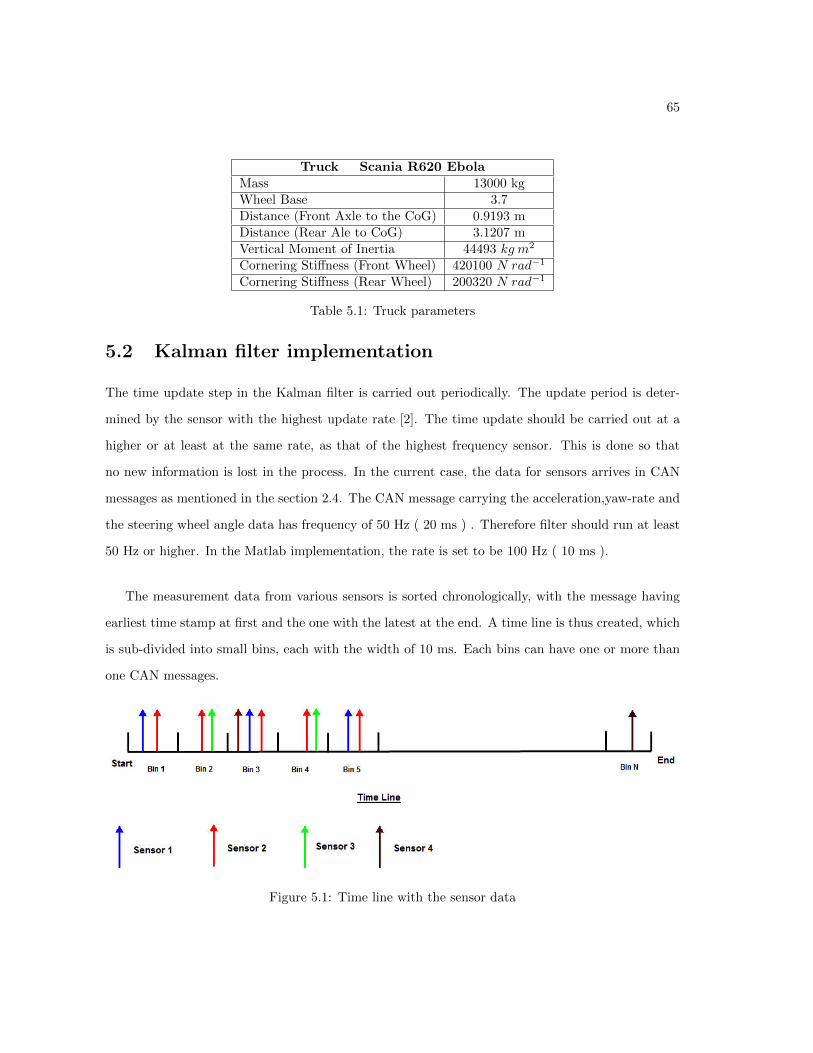
65
Truck Scania R620 EbolaMass 13000 kgWheel Base 3.7Distance (Front Axle to the CoG) 0.9193 mDistance (Rear Ale to CoG) 3.1207 mVertical Moment of Inertia 44493 kg m2
Cornering Stiffness (Front Wheel) 420100 N rad−1
Cornering Stiffness (Rear Wheel) 200320 N rad−1
Table 5.1: Truck parameters
5.2 Kalman filter implementation
The time update step in the Kalman filter is carried out periodically. The update period is deter-
mined by the sensor with the highest update rate [2]. The time update should be carried out at a
higher or at least at the same rate, as that of the highest frequency sensor. This is done so that
no new information is lost in the process. In the current case, the data for sensors arrives in CAN
messages as mentioned in the section 2.4. The CAN message carrying the acceleration,yaw-rate and
the steering wheel angle data has frequency of 50 Hz ( 20 ms ) . Therefore filter should run at least
50 Hz or higher. In the Matlab implementation, the rate is set to be 100 Hz ( 10 ms ).
The measurement data from various sensors is sorted chronologically, with the message having
earliest time stamp at first and the one with the latest at the end. A time line is thus created, which
is sub-divided into small bins, each with the width of 10 ms. Each bins can have one or more than
one CAN messages.
Figure 5.1: Time line with the sensor data
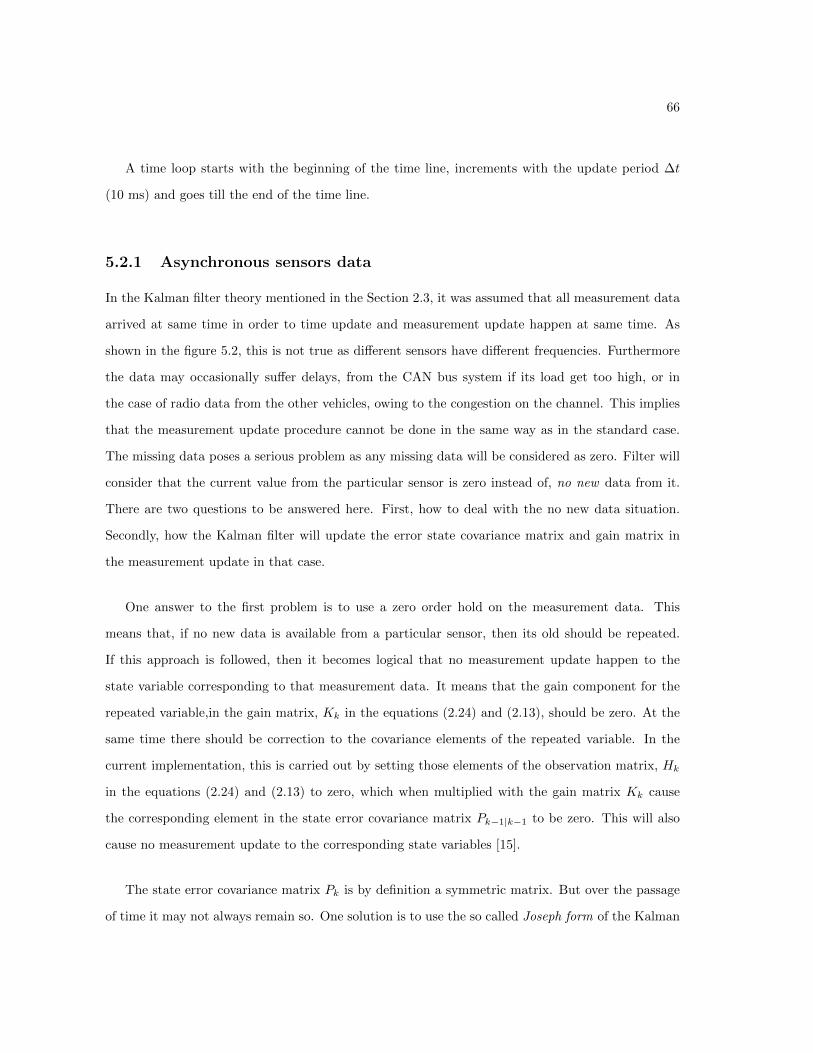
66
A time loop starts with the beginning of the time line, increments with the update period ∆t
(10 ms) and goes till the end of the time line.
5.2.1 Asynchronous sensors data
In the Kalman filter theory mentioned in the Section 2.3, it was assumed that all measurement data
arrived at same time in order to time update and measurement update happen at same time. As
shown in the figure 5.2, this is not true as different sensors have different frequencies. Furthermore
the data may occasionally suffer delays, from the CAN bus system if its load get too high, or in
the case of radio data from the other vehicles, owing to the congestion on the channel. This implies
that the measurement update procedure cannot be done in the same way as in the standard case.
The missing data poses a serious problem as any missing data will be considered as zero. Filter will
consider that the current value from the particular sensor is zero instead of, no new data from it.
There are two questions to be answered here. First, how to deal with the no new data situation.
Secondly, how the Kalman filter will update the error state covariance matrix and gain matrix in
the measurement update in that case.
One answer to the first problem is to use a zero order hold on the measurement data. This
means that, if no new data is available from a particular sensor, then its old should be repeated.
If this approach is followed, then it becomes logical that no measurement update happen to the
state variable corresponding to that measurement data. It means that the gain component for the
repeated variable,in the gain matrix, Kk in the equations (2.24) and (2.13), should be zero. At the
same time there should be correction to the covariance elements of the repeated variable. In the
current implementation, this is carried out by setting those elements of the observation matrix, Hk
in the equations (2.24) and (2.13) to zero, which when multiplied with the gain matrix Kk cause
the corresponding element in the state error covariance matrix Pk−1|k−1 to be zero. This will also
cause no measurement update to the corresponding state variables [15].
The state error covariance matrix Pk is by definition a symmetric matrix. But over the passage
of time it may not always remain so. One solution is to use the so called Joseph form of the Kalman
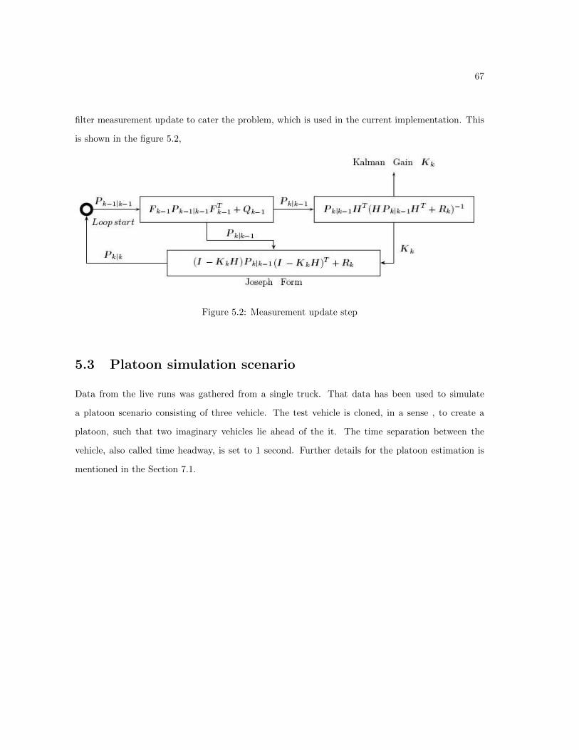
67
filter measurement update to cater the problem, which is used in the current implementation. This
is shown in the figure 5.2,
Figure 5.2: Measurement update step
5.3 Platoon simulation scenario
Data from the live runs was gathered from a single truck. That data has been used to simulate
a platoon scenario consisting of three vehicle. The test vehicle is cloned, in a sense , to create a
platoon, such that two imaginary vehicles lie ahead of the it. The time separation between the
vehicle, also called time headway, is set to 1 second. Further details for the platoon estimation is
mentioned in the Section 7.1.

Chapter 6
Single Vehicle Estimation Results
Chapter 3 described the two single vehicle models studied in this thesis. These included the kine-
matic model and a dynamic Bicycle model. This chapter describes the results for the single vehicle
estimation using both models. State estimation was done for two types of vehicle maneuvers, one
mainly along straight track and other in tight turnings. This is done in order to closely study the
relative performance of the two models in two distinct scenarios. The test runs were performed
on the Scania main test track. This chapter is divided in to three section. Estimation results for
straight run using both models are mentioned in the Section 6.1. Section 6.2 describes the results for
the turning maneuvers. In both of these sections, there are subsections, each describing the results
of a set of related estimated parameters. Finally in the section 6.3, a comparative analysis is done
for the performance of the two models.
6.1 Straight run results
The track was mentioned in the figure 3.5, which comprises of a combination of uphill, down hill,
gentle turns and straight runs. Test was conducted with truck running on different speed profile
along the track. The track itself starts at a slightly uphill position, then its goes down and starts to
turn to left gently. From there it is a fairly plain stretch of road. Then the track goes up and turns
left such that the it has maximum height in the middle. Its direction reverses and it goes down in
parallel to the opposite up going side. Finally the track circuit is closed at the point where it starts.
In the following subsections, the results of the kinematic and Bicycle models are presented along
side with each other.
68

69
6.1.1 Position estimates
Figure 6.1 shows the estimated trajectory in the local tangent or ENU frame. The data from GPS
receiver is in the geodetic ECEF reference frame, that has to be converted to the local tangent frame
using equation (2.6) and (2.5) before feeding it in the Kalman filter. The test run is 261 second long
and with an artificial GPS outage of 10 seconds occurring between 218th second and 228th second.
Also the track starts turning in counter clock-wise direction around 142nd seconds until it completely
reverses the direction about 160th seconds. The red crosses are the GPS position estimate used as
the observations and the blue solid line indicates the estimated position.
Figure 6.1: Estimated trajectory using the EKF with bicycle model
Also the number of visible satellites is plotted in the figure 6.2
Figure 6.2: Number of visible satellites
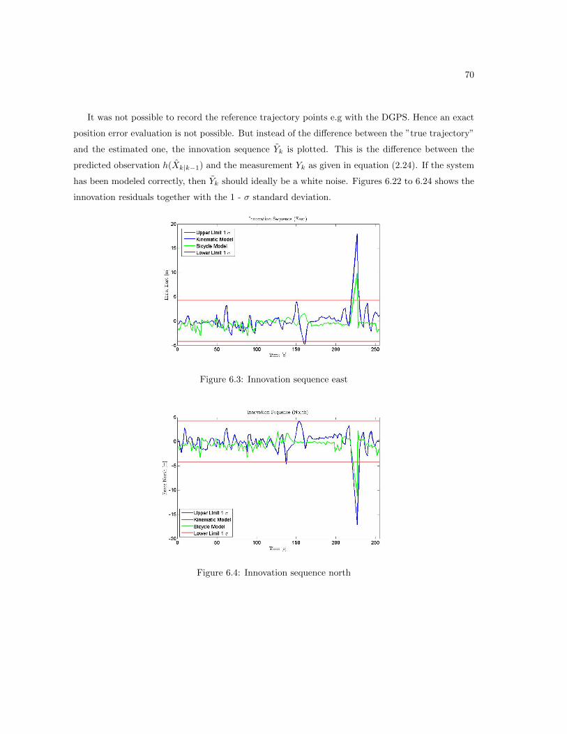
70
It was not possible to record the reference trajectory points e.g with the DGPS. Hence an exact
position error evaluation is not possible. But instead of the difference between the ”true trajectory”
and the estimated one, the innovation sequence Yk is plotted. This is the difference between the
predicted observation h(Xk|k−1) and the measurement Yk as given in equation (2.24). If the system
has been modeled correctly, then Yk should ideally be a white noise. Figures 6.22 to 6.24 shows the
innovation residuals together with the 1 - σ standard deviation.
Figure 6.3: Innovation sequence east
Figure 6.4: Innovation sequence north

71
Figure 6.5: Innovation sequence up
It can be seen from the above figures that the, for most of the time, the error in the East
and North position estimates is bounded by the standard deviation or 1σ bound, defined in Section
3.2.3. Exception happens between 218 and 228 second when there is an GPS outage. The innovation
sequence for the position estimates for both models actually over shoots the 1σ limit, but the bicycle
model due to its lateral dynamics estimation capability, performs better than the kinematic model.
Also during the turn which occurs between the 143rd and 160th second, the bicycle models again
has a lower error than the kinematic model as sufficient lateral forces are generated then, which
causes the vehicle to slip. Kinematic model cannot track this side slip and hence fares worse. In
the ideal case the innovation sequences should be white noises, but in the current case they are not.
The reason is that the position values i.e. Longitude and the Latitude used by the filters in the
estimation process are themselves the output of another Kalman filter inside the GPS receiver. This
induces a certain correlation in the position values that makes the innovation here non-white.
6.1.2 Velocities and Speed scale factor estimates
The longitudinal velocity, speed scale factor estimates and innovation sequences for two models are
shown in the figures 6.6 to 6.8.

72
Figure 6.6: Longitudinal velocities comparison
Figure 6.7: Speed scale factor
The WSS vehicle speed from the CAN, GPS ground speed and the two longitudinal velocities
estimates are plotted together in the figure 6.6. WSS speed is greater than the GPS speed, which is
used as the reference speed by EKFs running on the two models. The difference is estimated as the
speed scale factor which settles around a mean value of 22× 10−3. Also the innovation sequence for
the velocity is given by,

73
Figure 6.8: Longitudinal velocity innovation sequences
Lateral Velocity for the test vehicle is shown in the figure 6.9.
Figure 6.9: Lateral velocity
Lateral velocity has quite significant value when the vehicle turns as well as at the start and the
end of the recording. As it was mentioned that the track goes up and down hill, in the middle as
well in the start and the end. This creates a vertical component of the velocity. Vertical velocity is
given by the figure 6.10,

74
Figure 6.10: Vertical velocity
6.1.3 Acceleration and Acceleration bias estimates
Longitudinal Acceleration which is also tracked a states by the two models. Its estimates are shown
in the figure 6.11.
Figure 6.11: Longitudinal acceleration
The acceleration signal from the CAN bus is very noisy. Therefore it need to be filtered which
is done here by the two filters.
Lateral acceleration is used as an observation by the bicycle model. Here the acceleration signal
and its associated bias signal are shown in the figure 6.12 and 6.13.
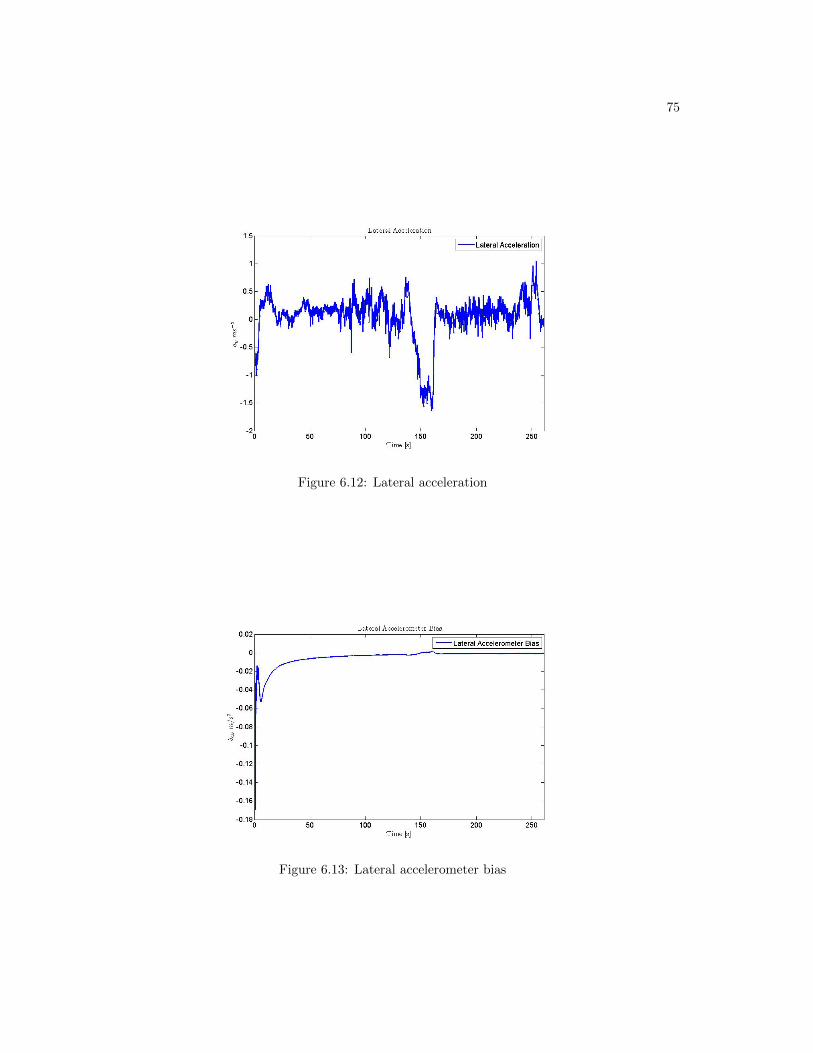
75
Figure 6.12: Lateral acceleration
Figure 6.13: Lateral accelerometer bias
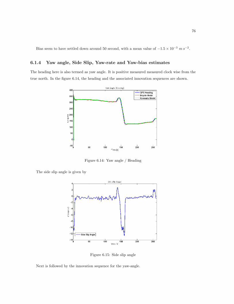
76
Bias seem to have settled down around 50 second, with a mean value of −1.5× 10⁻³ ms−2.
6.1.4 Yaw angle, Side Slip, Yaw-rate and Yaw-bias estimates
The heading here is also termed as yaw angle. It is positive measured measured clock wise from the
true north. In the figure 6.14, the heading and the associated innovation sequences are shown.
Figure 6.14: Yaw angle / Heading
The side slip angle is given by
Figure 6.15: Side slip angle
Next is followed by the innovation sequence for the yaw-angle.

77
Figure 6.16: Yaw angle innovation sequences
The innovation sequence for the heading estimates from the Kinematic model, as evident from
the above figure, some what resembles the side slip angle which is estimated by the Bicycle model.
The reason is the fact that the side slip is, by definition the difference of the GPS heading and the
yaw-angle tracked by the EKF as defined in the Section 3.3.1. Also the innovation for the bicycle
model is the difference of the GPS heading and the side slip angle and yaw-angle combined i.e.
ψbicycle = ψgps − (ψ + β) (6.1)
The yaw rate and the gyro bias are mentioned in the figures 6.17 and 6.18
Figure 6.17: Yaw rate

78
Figure 6.18: Yaw rate gyro bias
In the above figure, the gyro bias seems to have settled down around 2.73× 10⁻⁴, in about 180
seconds. Also the wheel steering angle is used as a control input by the bicycle model. It is not
directly measured but instead the steering wheel angle is measured and converted to the desired
angle by the non-linear relationship mentioned in the figure 2.4.4.
Figure 6.19: Wheel steering angle

79
6.2 Turning maneuver results
Bicycle model efficiently tracks the lateral dynamics of the vehicle. This helps in accurate estimation
of the vehicle position. This can be best seen when there are significant lateral forces present, as
in the case of constant cornering or turning. A second test was performed where the vehicle under
went constant turning for significant period of time. No GPS outage happened or was induced. This
section of the chapter deals with the estimation results for the such turning maneuver.
6.2.1 Position estimates
The estimated trajectories by the models, together with the GPS fixes are shown in the figures 6.20
and 6.21,
Figure 6.20: Estimated trajectory using the EKF with bicycle model
Figure 6.21: Estimated trajectory using the EKF with kinematic model

80
Innovation sequences for the position are shown the figures 6.22 to 6.24.
Figure 6.22: Innovation sequence east
Figure 6.23: Innovation sequence north

81
Figure 6.24: Innovation sequence up
Here the actual merits of the bicycle model come to full light. It can be seen that while turning
the estimates of the kinematic model goes quite off-course, sometimes even crossing the 1σ bound,
while the estimates of the bicycle model are always inside the limits.
6.2.2 Velocities and Speed scale factor estimates
The longitudinal velocity, speed scale factor estimates and innovation sequences for two models are
shown in the figure 6.25
Figure 6.25: Longitudinal velocities comparison

82
As the vehicle is constantly turning therefore an accurate estimation of the speed scale factor is
not possible. The figure 6.26 depicts that.
Figure 6.26: Speed scale factor
Innovation Sequence for the longitudinal velocity is
Figure 6.27: Longitudinal velocity innovation sequences
Lateral Velocity is given by

83
Figure 6.28: Lateral velocity
It is quite apparent that, the lateral velocity generated during the turning, can not be simply
ignored. Otherwise position estimation accuracy can suffer significantly. The vertical velocity is
given in the figure 6.29,
Figure 6.29: Vertical velocity

84
6.2.3 Acceleration and Acceleration bias estimates
Longitudinal acceleration estimates are shown in the figure 6.30.
Figure 6.30: Longitudinal acceleration
Lateral Acceleration and Biases are given by
Figure 6.31: Lateral acceleration

85
Figure 6.32: Lateral accelerometer bias
As can be seen above, the lateral accelerometer bias assumes a constant value of 1.5× 10⁻⁴ after
22 seconds. Actually the bias estimation is stopped as soon as the turning is initiated. It is done as
during the turning the bias and the actual signal become indistinguishable from each other.
6.2.4 Yaw angle, Side Slip, Yaw-rate and Yaw-bias estimates
Heading from the GPS is given in the figure 6.33
Figure 6.33: GPS heading
As the heading contains several discontinuities, this has to be un-wrapped before it is given
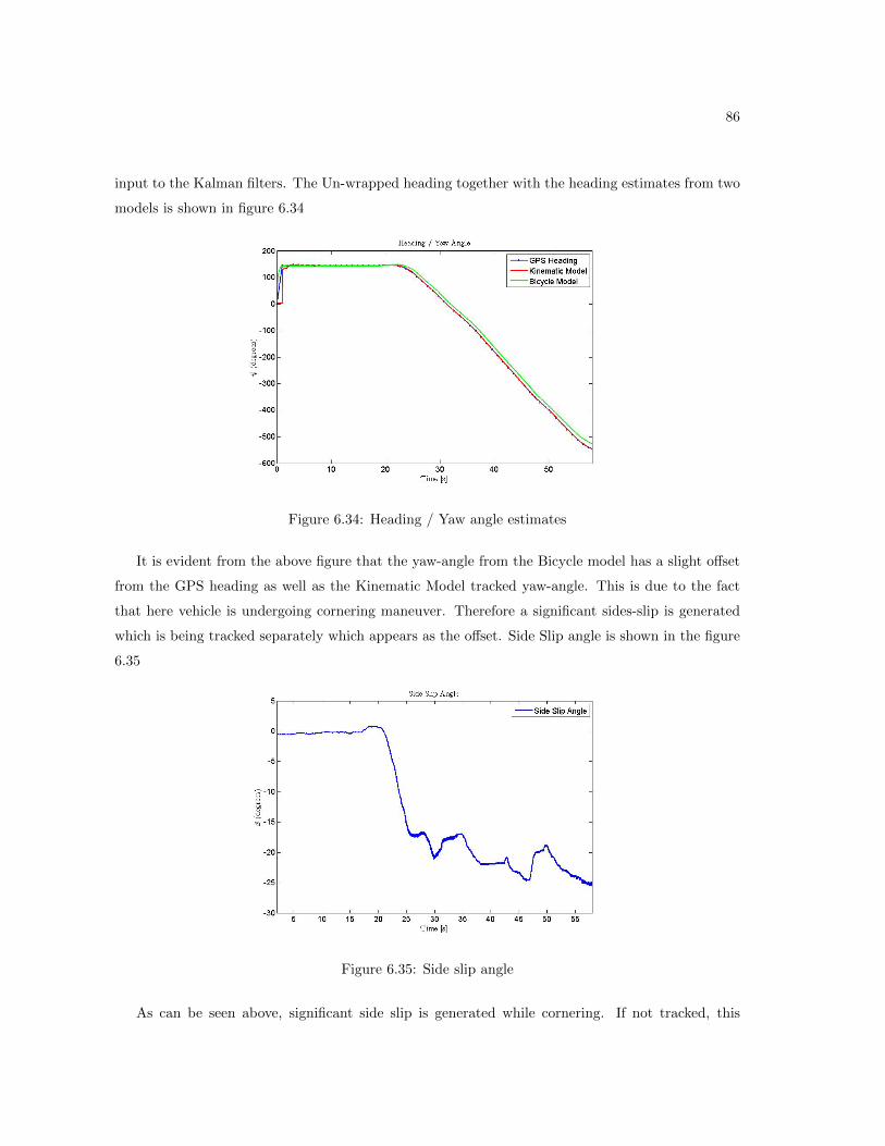
86
input to the Kalman filters. The Un-wrapped heading together with the heading estimates from two
models is shown in figure 6.34
Figure 6.34: Heading / Yaw angle estimates
It is evident from the above figure that the yaw-angle from the Bicycle model has a slight offset
from the GPS heading as well as the Kinematic Model tracked yaw-angle. This is due to the fact
that here vehicle is undergoing cornering maneuver. Therefore a significant sides-slip is generated
which is being tracked separately which appears as the offset. Side Slip angle is shown in the figure
6.35
Figure 6.35: Side slip angle
As can be seen above, significant side slip is generated while cornering. If not tracked, this

87
can lead to erroneous yaw-angle estimates that can have detrimental effects on the accuracy of the
position estimates. The innovation sequences for the yaw-angle estimates are shown in the figure
6.36.
Figure 6.36: Yaw angle innovation sequences
It can be observed that the innovation sequence for the yaw-angle for the bicycle model is almost
white while for the kinematic model, it resembles the curve for the side-slip angle. Yaw rate and
yaw bias are given in the figures 6.37 and 6.38,
Figure 6.37: Yaw rate

88
Figure 6.38: Yaw rate gyro bias
As in the case of the lateral accelerometer bias, here the gyro bias estimation is stopped as soon
the vehicle starts turning. Turning is said to happen when the yaw rate crosses a threshold of 5 degsec .
Wheel steering angle for the current maneuver is given in the figure 6.39,
Figure 6.39: Wheel steering angle

89
6.3 Discussion
In the sections above, the results for the two single vehicle models are discussed. The first of them
is the Kinematic model. This model is based on the equations of motion of a body in a plane. No
explicit knowledge of the vehicles parameters is required in this model. This is a autonomous model
that does not take any control input.
The second model studied is the bicycle model. This model takes into account the dynamic
forces acting on the vehicle. The vehicle dynamics are modeled similar to those of a bicycle, hence
the model takes its name. The prime focus of this model is to study the lateral dynamics of the
vehicle e.g. the side slip. It requires the knowledge of vehicle’s parameter. This model takes the
wheel steering angle as an input.To better analyze the performance of the two models, data from
two test tracks are studied. First is relatively a straight stretch of road for most of its part. The
second track is a tight maneuvering track where vehicle test undergoes constant cornering.
Kinematic model has limited number of states as compared to the bicycle model. It performance
is almost equivalent to that of the bicycle model when the vehicle is moving on straight stretch of
road. This can be sen from the results of the position and the heading innovation sequences. But
as soon the vehicle starts cornering, it generates lateral velocity that if not taken into account can
lead to larger errors in the position and the heading. Bicycle model estimates the lateral velocity
and the side slip angle that lead to accurate estimation of the above mentioned states.
On the other side, the bicycle model has more number of states and a larger state covariance
matrix than the kinematic model. It is in-fact a cascade of three sub-filters. Its operation requires
more computational resources than then simpler kinematic model. Also, vehicle parameters are
required to be known for its implementation. Therefore the choice of the model for the Ego vehicle
estimation depends on various factors like processing time constraints set by the hardware, the type
of motion track etc.

Chapter 7
Platoon Estimation Results
In the Chapter 5, two platoon vehicle models were discussed namely separate and joint estimation
models. This chapter describes their results . The chapter is divided in to five sections. In Section 7.1
the simulation strategy and design parameters are presented. Section 7.2 describes the results of the
inter vehicle distance estimation. Section 7.3 explains the results of the velocity / speed estimation.
It is divided into two sub sections. The first sub-section discusses the results for the relative velocity
while the second half deals with the results for the absolute speed estimation. Then in the section
7.4, the results for the acceleration are mentioned. Line bearing or the relative bearing results make
up the section 7.5 while the discussion on the performance of the two models is presented in the
Section 7.6.
7.1 Preface to platoon vehicle estimation
The test runs used to collect the data involved only one vehicle. Therefore in order to study the
models for the platoon and do simulations, a virtual platoon was created in the Matlab. It was
done by cloning the test (ego)vehicles two times such that two virtual vehicles, laying ahead of the
test vehicle, formed a platoon with it. Ego vehicle was termed as vehicle number 1 with the other
vehicles being 2 and 3. Measurement data from the Track 1 discussed in the Section 6.1 was used
in the simulation. This is shown in the figure 7.1,
90

91
Figure 7.1: Platoon trajectory
Observation vector for each vector included all the parameters that were supposed to be available
during the GCDC competition. This was mentioned in the Section 2.5. Radar data was generated
for the vehicle ahead. The relative distance between the vehicle was in terms of a constant time
separation also called time headway. It was chosen to be 1 second between each vehicle. This is
shown in the figure 7.2.
Figure 7.2: Time headway
As the signals from the platoon vehicles arrive via radio, they can get corrupted which results
in delayed or missing observations. The outage can last for several seconds. Therefore to study the

92
performance of the models in the outage, a radio loss of 10 seconds was simulated for both vehicles
at different time instances. For the vehicle 2 which is also the Vehicle Ahead, the radio outage was
simulated between 90th and 100th second, while for the vehicle 3 it was between 220th and 230th
second.
7.1.1 Radar modeling
Radar data is modeled by taking the data of the vehicle with out radio outage and adding white
noise of small variance to it.
7.2 Relative distance
First the East and the North components of the estimated relative distance vector ∆p21e and ∆p21n
for the vehicle no.2 are shown.
Figure 7.3: Relative distance components for vehicle no. 2 ∆p21e and ∆p21n

93
Similarly for the vehicle no.3, ∆p31e and ∆p31n are given in figure 7.4,
Figure 7.4: Relative distance components for vehicle no. 3 ∆p31e and ∆p31n
Figure 7.5 shows the estimated relative distances in meters, by the two models,
Figure 7.5: Relative distance to the vehicle no. 2 ∆d12
In the figure 7.5, three variables are plotted. The first is the distance estimated by the separate
estimation model ∆dseparate21 . The second is the same but with radar data fusion ∆dseparate,radar21 .
Finally the third is the relative distance estimated by the joint estimation model ∆djoint21 . From the
visual inspection it is obvious that the third technique fares better than the other two. In order
to evaluate the performance of the model,the difference of three relative distances and the jointly
estimated relative distance are plotted.

94
Figure 7.6: Difference of relative distances with radio outage and without outage, Vehicle No.2
It becomes clear that the joint estimation technique is better than the separate estimation with
and with our radar fusion. In the similar way the relative distances for the third vehicle is plotted.
Figure 7.7: Relative distance to the vehicle no. 3 ∆d13
The performance of the joint estimation model is evidently superior to that of the separate
estimation model.

95
Figure 7.8: Difference of relative distances with radio outage and without outage, Vehicle No.3
7.3 Velocity / Speed
The speed section describes the results of the two models.
7.3.1 Absolute speed
First the absolute speed of the three vehicles is plotted. This includes the radar fusion for the vehicle
in front.
Figure 7.9: Absolute speed of vehicles
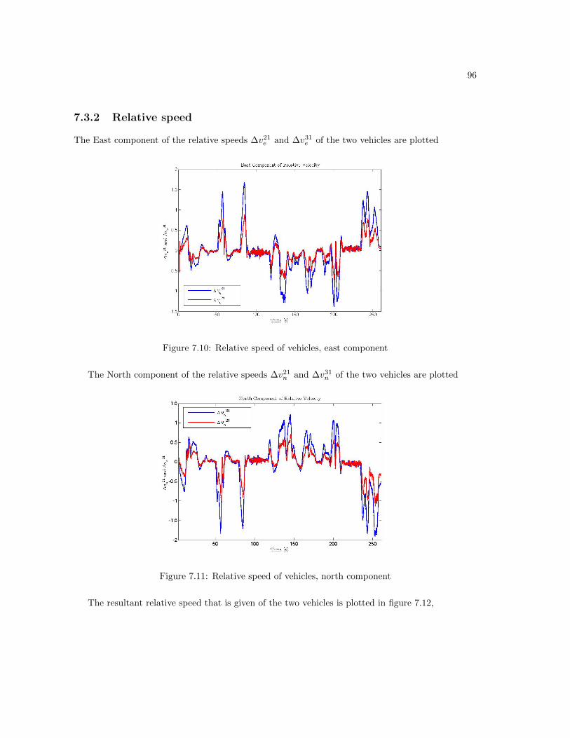
96
7.3.2 Relative speed
The East component of the relative speeds ∆v21e and ∆v31e of the two vehicles are plotted
Figure 7.10: Relative speed of vehicles, east component
The North component of the relative speeds ∆v21n and ∆v31n of the two vehicles are plotted
Figure 7.11: Relative speed of vehicles, north component
The resultant relative speed that is given of the two vehicles is plotted in figure 7.12,

97
Figure 7.12: Relative speed of vehicles
7.4 Relative heading (Line bearing)
Line bearing is used in calculating the relative distance of the vehicles in front to the Ego vehicle.
The results for the line bearing are shown in the figure 7.13
Figure 7.13: Relative bearing of vehicles
It is important to note that line bearing shows change while the vehicles are negotiating turn,
that is in the middle of the track.
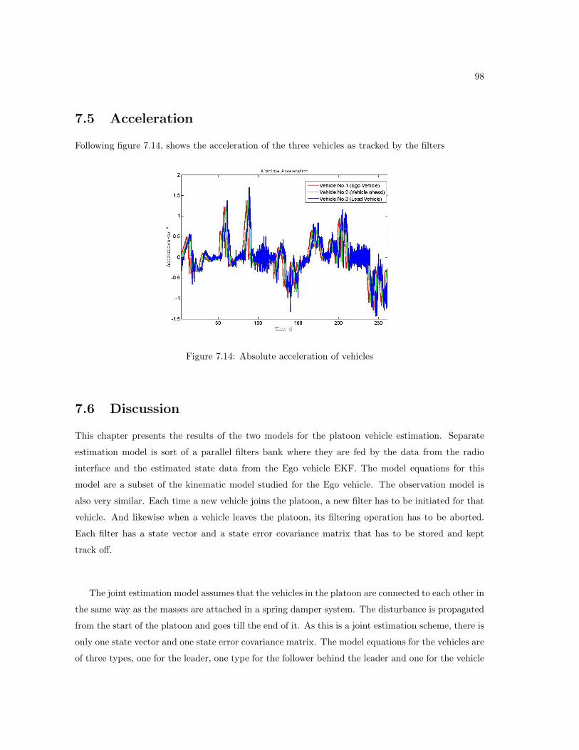
98
7.5 Acceleration
Following figure 7.14, shows the acceleration of the three vehicles as tracked by the filters
Figure 7.14: Absolute acceleration of vehicles
7.6 Discussion
This chapter presents the results of the two models for the platoon vehicle estimation. Separate
estimation model is sort of a parallel filters bank where they are fed by the data from the radio
interface and the estimated state data from the Ego vehicle EKF. The model equations for this
model are a subset of the kinematic model studied for the Ego vehicle. The observation model is
also very similar. Each time a new vehicle joins the platoon, a new filter has to be initiated for that
vehicle. And likewise when a vehicle leaves the platoon, its filtering operation has to be aborted.
Each filter has a state vector and a state error covariance matrix that has to be stored and kept
track off.
The joint estimation model assumes that the vehicles in the platoon are connected to each other in
the same way as the masses are attached in a spring damper system. The disturbance is propagated
from the start of the platoon and goes till the end of it. As this is a joint estimation scheme, there is
only one state vector and one state error covariance matrix. The model equations for the vehicles are
of three types, one for the leader, one type for the follower behind the leader and one for the vehicle

99
at the end. The model uses the data from the own vehicle as the control input. The observation
model is a linear one with the inputs from the radio, radar and the own vehicle estimated data. Each
time a vehicle joins the platoon, it is checked whether the vehicle is a new leader or a new follower.
The state model is accordingly selected. This effectively increases the size of the state vector and
the covariance matrix.
Performance of these models can be analyzed with different judging parameters. First comes
the track error of the states. The joint estimation model estimates all states including the relative
distance internally i.e. not after the filtration is done. This ensures that the estimation error is
theoretically always less than the separate estimation model. This is evident from the estimation
results. But this comes with a price to pay. The first is that there are in fact three not one sub-model
for the platoon vehicles as describes above. This adds to the complexity as each a vehicle joins or
leaves the platoon, it has to assigned a appropriate sub-model. The second is that as the number
of the vehicles in the platoon grow, the size of the state vector and the covariance matrix increase.
This can be seen that for each vehicle, there are seven parameters that are tracked by the EKF
using this model. While for low number of vehicles this is not a problem, as the size of platoon
increases, it becomes more time consuming to invert the matrix in the time update step of the EKF.
The inversion can be implemented in an efficient way but still it can be a bottle neck in the real
time working.
Finally, it can be said that the choice of the model is dependant on the platooning strategy e.g. if
the vehicles in the platoon can be limited, on the hardware on which the EKF is to be implemented
and finally the implementation strategy i.e. how the matrix inversion is performed.

Chapter 8
Conclusion and Future works
This is the final chapter of the thesis report. This includes a conclusion section that discuses the
main inferences of the thesis work. Finally it includes a future works section that summarizes the
possible future extension of the thesis study.
8.1 Conclusion
The purpose of this thesis was to define the specifications and study the strategies that could be
employed for the state estimation of single vehicle and of platoon. States are the variables that are
required by the vehicle controller for controlling the vehicle. In addition to that, GCDC defines a
set of information that needs to be exchanged between the vehicles via radio, which are also part of
the states to be estimated. Two types of states have been classified, first is the own vehicle state and
the other being the platoon states. Single vehicle states are used to represent the vehicles dynamic
information. Platoon states refer to the set of variables describing the dynamics of other vehicles in
the platoon, also called platoon-mates. Kalman filters have been employed for the state estimation.
Different models have been studied, both for representing the single vehicle and the vehicles in
platoon. For the single vehicle this includes the so called Kinematic model and the Bicycle model.
Kinematic model representation does not require the knowledge of the vehicles parameters, whereas
the application of the Bicycle model does. Also the bicycle model implementation is more involved
that the kinematic model. It seems a bit more computationally intensive. On the other hand, the
kinematic model suffers in terms of accuracy especially during the turning maneuvers. This can be
critical if the vehicle’s area of operation is not a straight stretch of road.
100

101
For the platoon state estimation, again two models are studied. The first is the separate estima-
tion model that estimates the states of each vehicle in the platoon individually. The second one is a
joint estimation model. It tries to estimates the states of all platoon vehicles as part of a single state
vector. Here again each model has its own particular advantages and disadvantages. The separate
estimation model is simple in its mathematical representation as compared to the joint estimation
method which is more complex. The processing time taken by the two depends upon the number of
vehicles in platoon. For less number of vehicles, both take almost almost equal amount of time but
as the size of platoon grows, so does the relative processing time taken by the joint model. But it
has better performance as compared to the former. Actually the decision of employing the model
depends upon the platooning strategies, and on the processing power available.
8.2 Future Work
Some of the possible future extensions that can be done on the basis of current work are being
mentioned below.
8.2.1 Inclusion of an IMU
The measurements used in the estimation were taken from the trucks CAN bus system. This included
only one lateral accelerometer and one yaw-rate gyro. It would be of great interest to incorporate a
3D Inertial measurement unit with a set 3 accelerometer and 3 gyros.
8.2.2 Four wheel model
A bicycle model has been studied together with a simple kinematic model. A four wheel vehicle
model can be studied and comparisons made between their performances.
8.2.3 Longer data set
Data set of maximum of 4.5 minutes was used. It would be nice to see the system behavior with the
data that also includes the start from the stand still and stop from a running condition.
8.2.4 More advanced platoon estimation models
Some more involved platoon estimation model can be studied, that might take into account the
delays on the radio network.
8.2.5 Real time implementation and testing
Finally, the whole work is most beneficial if it can be implemented and tested in real time.
Bibliography
[1] TNO, “Gcdc rules and technology final version 2.0, http://www.gcdc.net,” tech. rep., GCDC
organization, Feb 2011.
[2] J. A. Farrell, Professional Aided Navigation GPS with High Rate Sensors. New York: McGraw-
Hill, 2008.
[3] V. Antevski, “Heavy vehicle trajectory control,” Master’s thesis, Aeronautical and Vehicle
Engineering School, KTH Stockholm Sweden, 2011.
[4] J. F. King TinLeung, “Road vehicle state estimation using low-cost gps/ins,” Mechanical Sys-
tems and Signal Processing, vol. 25, no. 6, pp. 1988–2004, 2010.
[5] T. Gillespie, Fundamentals of Vehicle Dynamics. Warrendale: Society of Automotive Engineers,
1992.
[6] S.-Y. Yi and K.-T. Chong, “Impedance control for a vehicle platoon system,” Mechatronics,
vol. 15, no. 5, pp. 627–638, 2005.
[7] A. Schumacher, “Integration of a gps aided strapdown inertial navigation system for land ve-
hicles,” Master’s thesis, EE School, KTH Stockholm Sweden, 2006. report number XR-EE-SB
2006:006.
[8] J.Y.Wong, Theory of Ground Vehicle. John Wiley and Sons, 2001.
[9] J. R. David M. Bevly and J. C. Gerdes, “Integrating ins measurement with gps measurments
for continuous estimation of vehicle sideslip, roll and tire cornering stiffness,” IEEE Transaction
on Intelligent Transport System, 2006.
[10] M. B. David and P. Bradford, “Cascaded kalman filters for accurate estimation of multiple
biases, dead-reckoning navigation, and full state feedback control of ground vehicles,” IEEE
Transactions on Control Systems Technology, vol. 15, no. 2, pp. 199–208, 2007.
102

103
[11] K. J. B. Thomas A. Wenzel and M. V.Blundell, “Simplified extended kalman filter for automa-
tive state estimation,” Int H, Modelling, Identification and Control, vol. 3, no. 3, 2008.
[12] J. Kjellberg, “Implementing control algorithms for platooning based on v2v communication,”
Master’s thesis, EE School, KTH Stockholm Sweden, 2011. report number, XR-EE-RT
2011:008.
[13] F. Gustafsson, Statistical Sensor Fusion. Lund: Studentlitteratur, 2010.
[14] P.A.Cook, “Conditions for string stability,” Systems and Control Letters, vol. 54, no. 10,
pp. 991–998, 2005.
[15] R. L. Thorne, “Asynchronous data fusion for auv navigation using extended kalman filter,” Mas-
ter’s thesis, Naval Postgraduate School, Monterey California, 1997. report number, 19971122-
133.