1

Spectral analysis of rock samples from East Suriname

using the Spectral Evolution PSR+

- Building a spectral library of rock samples -

Shannon de Roos & Steven M. de Jong

24 November 2017

Department of Physical Geography

Utrecht University, The Netherlands

2

3

ABSTRACT

Spectral signatures of minerals and rocks can be used to determine mineral compositions for specific

areas and can function as a useful aid for remote sensing image interpretation. In this study, the aim

is to build a spectral library of common rocks and minerals for the region of East Suriname,

particularly the Greenstone belt, and to test the performance of the recently purchased

spectroradiometer PSR+. The samples that were used for building the spectral library were selected

from multiple collections from the geological department of Naturalis, Leiden. The samples were

selected based on the overlap of their location of origin with the study area and on their relation with

mining sources bauxite and gold. For the evaluation of the PSR+ spectroradiometer, samples from

the Peyne area, southern France, were used. Samples from the Peyne area consisted of seven different

rock samples, from nine different locations. Most minerals and rocks of the Suriname collection

showed impurities by iron or iron- bearing minerals due to weathering and other causes. The spectral

signatures of the metasomatic rock sample showed the significant presence of the mineral muscovite

and it appeared that the hornfels sample contained the same green epidote mineral as the greenstone

sample.

This spectral library was created as an aid for remote sensing image interpretation for images of

Suriname. However, geological image interpretation in Suriname would not be easy, due to the vast

amount of vegetation and deep weathering of exposed rock and the low availability of cloud-free

images.

Evaluation of the measurements of the PSR+3500 show variations (or noise) in the optical range of

the spectrum measured by the first detector. The rippling effect (peaks/valleys) that was created in

this range 400-1100nm, influences the spectral reflectance measurements of the rock samples.

Additionally, peaks were visible in the spectral signatures at the wavelength range of the transition

of the detectors. To improve the spectral reflectance curves, which is mostly needed for the optical

part of the spectrum, the noise of the detectors and the transition in detectors should be as small as

possible.

i

4

TABLE OF CONTENTS

ABSTRACT ....................................................................................................................................................................................................... i

ACKNOWLEDGEMENT ........................................................................................................................................................................... iii

1 INTRODUCTION .................................................................................................................................................................................... 1

1.1 Spectral signatures.................................................................................................................................................................... 1

1.1.1 Absorption features ................................................................................................................................................................. 1

1.2 Spectral evolution PSR+.......................................................................................................................................................... 2

1.3 Study areas ................................................................................................................................................................................... 3

1.3.1 Eastern Suriname ...................................................................................................................................................................... 3

1.3.2 La Peyne, France ........................................................................................................................................................................ 5

1.4 Research objectives .................................................................................................................................................................. 6

2 METHODS................................................................................................................................................................................................. 7

2.1 Rock and mineral samples ..................................................................................................................................................... 7

2.1.1 Suriname samples ..................................................................................................................................................................... 7

2.1.2 Peyne samples ............................................................................................................................................................................ 8

2.2 DARWin SP application software ....................................................................................................................................... 9

2.2.1 Instrument control panel ....................................................................................................................................................... 9

2.2.2 Main menu .................................................................................................................................................................................. 10

2.2.3 The scan ....................................................................................................................................................................................... 11

3 RESULTS ................................................................................................................................................................................................. 13

3.1 Spectral analysis of the Suriname Collection .............................................................................................................. 13

3.1.1 Minerals ....................................................................................................................................................................................... 13

3.1.2 Sedimentary rocks .................................................................................................................................................................. 21

3.1.3 Metamorphic rocks ................................................................................................................................................................. 28

3.1.4 Igneous rocks ............................................................................................................................................................................ 37

3.2 Analysis of the spectroradiometer PSR+3500 ............................................................................................................ 41

3.2.1 Accuracy instrument.............................................................................................................................................................. 41

3.2.2 Effect accuracy on measurements ................................................................................................................................... 42

3.2.3 Number of scans ...................................................................................................................................................................... 43

3.2.4 Contact probe ............................................................................................................................................................................ 44

4 DISCUSSION .......................................................................................................................................................................................... 47

5 CONCLUSION ........................................................................................................................................................................................ 48

6 REFERENCES ........................................................................................................................................................................................ 49

ii

5

ACKNOWLEDGEMENT

This research would not have been possible without the samples from Suriname, which we were able

to obtain thanks to the geological collections of Natuur Historisch Museum Naturalis, Leiden and the

help of Arike Gill, who sorted out the samples that we requested. I would also like to thank Ing. Marcel

van Maarseveen, for his help regarding the PSR+ Spectroradiometer and the DARWin software. I

want to thank drs. Maarten Zeylmans van Emmichoven for being willing to act as my second

supervisor.

iii

1

1 INTRODUCTION

1.1 Spectral signatures

Spectral signatures of minerals and rocks can be used to determine mineral compositions for specific

areas and can be an useful aid for remote sensing image interpretation. In this study, a spectral library

of the Greenstone belt region in East Suriname is build and the performance of the recently purchased

PSR+ spectroradiometer of the University of Utrecht is tested. For the evaluation of the PSR+

spectroradiometer, samples from the Peyne area, southern France, were used.

Each object contains a reflectance spectrum. When lights incidents on this object, it interacts with it,

where parts of the light spectrum are reflected and other parts absorbed (van der Meer & de Jong,

2006). Reflectance is therefore defined as the ratio of intensity of light reflected from a sample, to the

intensity of light incident upon it (van der Meer & de Jong, 2006). For many years, information about

the earth surface has been gained from reflectance spectra, as it is a rapid and non-destructive method

to study the mineralogy of rocks (van der Meer& de Jong, 2006). Apart from the wavelength bands in

the optical part of the wavelength spectrum (blue;400-500nm, green;500-600 nm, red;600-700 nm),

Near infrared (NIR; 700-1500 nm) and short wave infrared (1500-3000 nm) are of importance when

analysing spectra of minerals (van der Meer & de Jong, 2006).

1.1.1 Absorption features

Absorption features are determined by electronic transition and charge transfer processes,

associated with transition metal ions, but also by vibrational processes of H2O and OH- molecules (van

der Meer& de Jong, 2006). Properties of these absorption features include the position, shape, depth,

width and asymmetry and are the result of the specific crystal structure in which the absorbing

element resides and by the chemical structure of the mineral (van der Meer& de Jong, 2006).

Absorption features are therefore directly related to the mineral composition of a rock fragment.

The most common features in the mineral spectra are caused by the electronic process called the

crystal field effect (van der Meer & de Jong, 2006). This occurs due to unfilled electron shells of

transition metals. It appears that in an isolated ion, these transition metals have identical energies,

but that these energy levels are split when the atom is situated in a crystal field (van der Meer & de

2

Jong, 2006). When different energy levels are created, it becomes possible for an electron to move

from a lower to higher energy level. To do this, it needs the energy of a photon that equals the energy

of the difference between these energy levels. Absorption bands can also be caused by charge transfer,

for example when Fe2+ transforms into Fe3+. The resulting absorption bands from charge transfers

are characteristic to its mineralogy (van der Meer & de Jong, 2006).

Absorption features can also be created by vibrations of the strings that bonds atoms to form

molecules (van der Meer & de Jong, 2006). Vibrations are generated when energy is absorbed by the

molecule in its ground state. The frequency of the vibration is dependent on the strength of the

strings. Because vibrations cost little energy, absorption features occur at high wavelengths, in the

infrared region (800-2500 nm), and are deep and narrow (van der Meer & de Jong, 2006). In minerals,

absorption features due to vibrational processes are mainly caused by water and hydroxyl molecules,

but also by carbonate and sulphate.

Additionally, absorption band depth is influenced by the grain size of a particle. It decides the amount

of light that is absorbed or scattered (van der Meer & de Jong, 2006). In general, smaller grains cause

higher albedos, whereas in larger grains the absorption is larger, as the internal path for photon

absorption is longer (van der Meer & de Jong, 2006).

1.2 Spectral evolution PSR+

The spectroradiometer PSR+3500, recently purchased by the University of Utrecht, has a spectral

range of 350 to 2500 nm and a high spectral resolution, varying from 3nm to 8nm (Spectral Evolution,

2012). The spectral range is measured with three detectors, which are presented together with the

spectral resolutions at Full Width Half Maximum in table 1.1.

Table 1.1 Detectors and spectral resolutions (Full Width at Half Maximum) , of the spectroradiometer PSR+.

Detector Type Range (nm) Spectral resolution (FWHM)

1 512 element Si photodiode array 350-1000 3 nm at 700 nm

2 256 element extended InGaAs photodiode

array

970-1910 8 nm at 1500 nm

3 256 element extended InGaAs photodiode

array

1900-2550 6 nm at 2100 nm

3

The PSR+3500 is provided with a contact leaf clip and a contact probe, which allows one to measure

the spectral radiance of rock fragments and vegetation leaves. The contact probe contains its own

light source and has a scan button. The scan can therefore be made while holding the contact probe,

but it is also possible to take the target scan from the computer using the DARWin software. The

instrument is further provided with lenses of varying angles (1-5°, 8° & 10°), so that a wide range of

objects can be measured.

For further information about the instrument, the site of Spectral Evolution is recommended;

http://www.spectralevolution.com/spectroradiometer_PSR_plus.html.

1.3 Study areas

1.3.1 Eastern Suriname

The mining sector in Suriname is the most important contribution to the country’s economy, with its

main focus on the metals gold, which accounted around 60% of the economic export in 2010, and

bauxite, which contributed around a quarter to the total export (Briegel, 2012). Suriname belongs to

one of the top ten bauxite sources in the world (Mobbs, 2016).

Some large bauxite and gold mines are found in eastern Suriname, where the primary bauxite mines

are located in the North in Lelydorp and Coermotibo (Haalboom, 2012). However, as these mines are

nearing depletion, new bauxite mines, such as the Kaaimangrassie and Klaverblad mines are opened

(Haalboom, 2012).

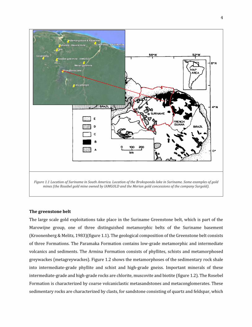
Large scale gold exploitation takes place in east Suriname, around the Brokopondo lake (figure 1.1).

Some examples of gold mines are the Rosebel gold mine, owned by IAMGOLD and the Merian gold

concessions of the company Surgold.

4

Figure 1.1 Location of Suriname in South America. Location of the Brokopondo lake in Suriname. Some examples of gold mines (the Rosebel gold mine owned by IAMGOLD and the Merian gold concessions of the company Surgold).

The greenstone belt

The large scale gold exploitations take place in the Suriname Greenstone belt, which is part of the

Marowijne group, one of three distinguished metamorphic belts of the Suriname basement

(Kroonenberg & Melitz, 1983)(figure 1.1). The geological composition of the Greenstone belt consists

of three Formations. The Paramaka Formation contains low-grade metamorphic and intermediate

volcanics and sediments. The Armina Formation consists of phyllites, schists and metamorphosed

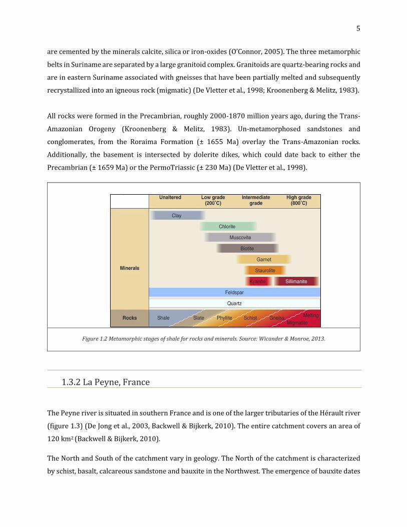
greywackes (metagreywackes). Figure 1.2 shows the metamorphoses of the sedimentary rock shale

into intermediate-grade phyllite and schist and high-grade gneiss. Important minerals of these

intermediate-grade and high-grade rocks are chlorite, muscovite and biotite (figure 1.2). The Rosebel

Formation is characterized by coarse volcaniclastic metasandstones and metaconglomerates. These

sedimentary rocks are characterized by clasts, for sandstone consisting of quartz and feldspar, which

5

are cemented by the minerals calcite, silica or iron-oxides (O’Connor, 2005). The three metamorphic

belts in Suriname are separated by a large granitoid complex. Granitoids are quartz-bearing rocks and

are in eastern Suriname associated with gneisses that have been partially melted and subsequently

recrystallized into an igneous rock (migmatic) (De Vletter et al., 1998; Kroonenberg & Melitz, 1983).

All rocks were formed in the Precambrian, roughly 2000-1870 million years ago, during the Trans-

Amazonian Orogeny (Kroonenberg & Melitz, 1983). Un-metamorphosed sandstones and

conglomerates, from the Roraima Formation (± 1655 Ma) overlay the Trans-Amazonian rocks.

Additionally, the basement is intersected by dolerite dikes, which could date back to either the

Precambrian (± 1659 Ma) or the PermoTriassic (± 230 Ma) (De Vletter et al., 1998).

Figure 1.2 Metamorphic stages of shale for rocks and minerals. Source: Wicander & Monroe, 2013.

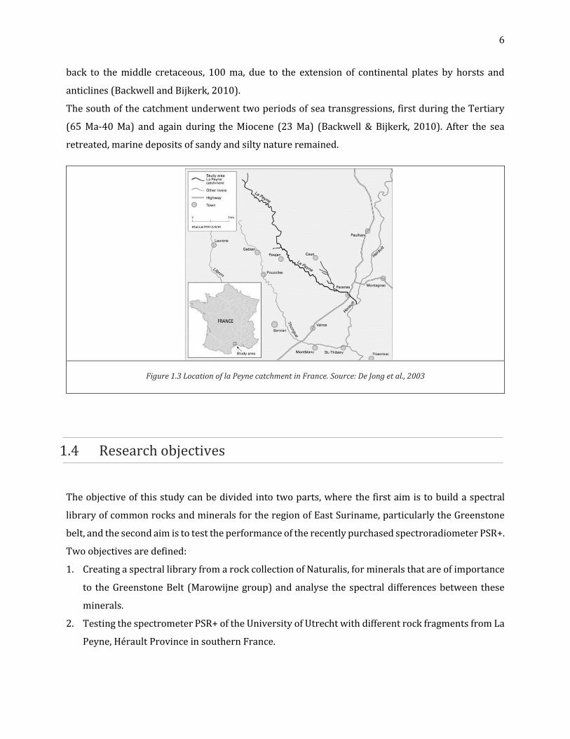
1.3.2 La Peyne, France

The Peyne river is situated in southern France and is one of the larger tributaries of the Hérault river

(figure 1.3) (De Jong et al., 2003, Backwell & Bijkerk, 2010). The entire catchment covers an area of

120 km2 (Backwell & Bijkerk, 2010).

The North and South of the catchment vary in geology. The North of the catchment is characterized

by schist, basalt, calcareous sandstone and bauxite in the Northwest. The emergence of bauxite dates

6

back to the middle cretaceous, 100 ma, due to the extension of continental plates by horsts and

anticlines (Backwell and Bijkerk, 2010).

The south of the catchment underwent two periods of sea transgressions, first during the Tertiary

(65 Ma-40 Ma) and again during the Miocene (23 Ma) (Backwell & Bijkerk, 2010). After the sea

retreated, marine deposits of sandy and silty nature remained.

Figure 1.3 Location of la Peyne catchment in France. Source: De Jong et al., 2003

1.4 Research objectives

The objective of this study can be divided into two parts, where the first aim is to build a spectral

library of common rocks and minerals for the region of East Suriname, particularly the Greenstone

belt, and the second aim is to test the performance of the recently purchased spectroradiometer PSR+.

Two objectives are defined:

1. Creating a spectral library from a rock collection of Naturalis, for minerals that are of importance

to the Greenstone Belt (Marowijne group) and analyse the spectral differences between these

minerals.

2. Testing the spectrometer PSR+ of the University of Utrecht with different rock fragments from La

Peyne, Hérault Province in southern France.

7

2 METHODS

2.1 Rock and mineral samples

Two collections were created with the PSR+ spectroradiometer. The rock sample collection of eastern

Suriname was measured and compared to mineral spectra from the USGS spectral library (SPecLib

V6) which was available in ENVI 5.2. For most rock sample analysis, the rock and mineral description

from several sites that provides mineral rock information have been used: Rocks & minerals, by

O’Connor (2005); minerals.net, by Friedman (1997-2017); Mindat (n.d.).

Samples from the Peyne area consisted of seven different rock samples, from nine different locations.

This collection was not analysed in detail, but mainly used to test the performance of the PSR+3500

instrument and the DARWin application software.

2.1.1 Suriname samples

The samples that were used for building the spectral library were selected from multiple collections

from the geological department of Naturalis, Leiden. The samples were selected based on the overlap

of the location of origin with the study area and on their relation with mining sources bauxite and

gold. Some samples were not found in Northeast Suriname, but these samples were chosen because

they are very common rocks in Suriname or because of their interesting spectral signatures.

Most samples were used from the collection of J.W. Brinck (1950-1955), during his expedition about

gold deposits. These samples were taken from the region around the Brokopondo lake. The presence

of gold is dependent on the Formation in which it has been mineralized. Brinck (1956) found gold

attached to mostly quartz, blue quartz and pyrite, and stated that ferberite is a valuable indication of

gold.

Bauxite, hematite and kaolinite samples were used from a collection of the TU Hogeschool Delft

(collection date unknown). These samples originated from the bauxite mines Rorac and Para, situated

above the study area, Northeast Suriname. Other samples were used from collections of R.H.

Verschure (n.d.), F. Voltz (± 1931), J.F. van Kersen (1955) and two gneiss samples from the Bakhuys

expedition (n.d.), from West Suriname. The full list of the collected samples, description and specific

8

location can be found as an Appendix of the Suriname collection in the form of an excel sheet. This

appendix also contains pictures of the samples along with the measured spectra. Exact locations were

found using Google Earth. The samples are from old expeditions (50-100 years ago), therefore,

specific locations were often difficult to find. For a few samples the locations could not be traced back.

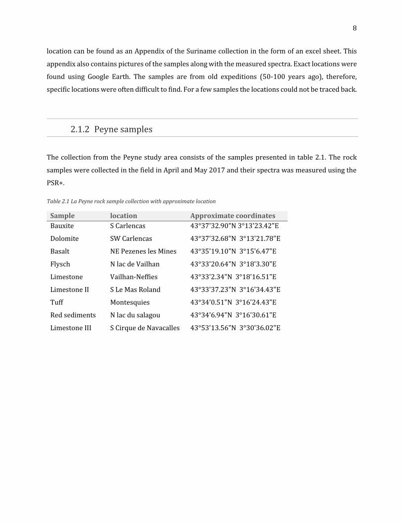
2.1.2 Peyne samples

The collection from the Peyne study area consists of the samples presented in table 2.1. The rock

samples were collected in the field in April and May 2017 and their spectra was measured using the

PSR+.

Table 2.1 La Peyne rock sample collection with approximate location

Sample location Approximate coordinates

Bauxite S Carlencas 43°37'32.90"N 3°13'23.42"E

Dolomite SW Carlencas 43°37'32.68"N 3°13'21.78"E

Basalt NE Pezenes les Mines 43°35'19.10"N 3°15'6.47"E

Flysch N lac de Vailhan 43°33'20.64"N 3°18'3.30"E

Limestone Vailhan-Neffies 43°33'2.34"N 3°18'16.51"E

Limestone II S Le Mas Roland 43°33'37.23"N 3°16'34.43"E

Tuff Montesquies 43°34'0.51"N 3°16'24.43"E

Red sediments N lac du salagou 43°34'6.94"N 3°16'30.61"E

Limestone III S Cirque de Navacalles 43°53'13.56"N 3°30'36.02"E

9

2.2 DARWin SP application software

2.2.1 Instrument control panel

The PSR+ instrument can be connected to the PC with an USB cable, via a Bluetooth adapter. When

the instrument is connected, the DARWin software can be used. Each time the software is opened, the

instrument has to be configured. This is done with the “Inst. Control” button on the toolbar. First, the

right COM port has to be selected from the pull-down menu and then the PC should be connected to

the instrument. A successful connection should display the text “COM# opened” right next to the

connect button. In the upper right corner, the active instrument will be displayed

(PSR+3500_serialnumber) and the instruments parameters will be loaded. After the connection is

made, the type of measurement can be selected. Measurement options include: Direct Energy, which

can be used when radiance and irradiance are of interest, and reflectance or absorbance, both for

ratio measurements.

It should be noted that when the option Direct Energy is chosen, the reflectance values will not be

saved. So when re-opening the saved file of the scan, only the reference and target scan can be

displayed. In this study, the performance of the instrument is analysed, therefore the option Direct

energy is chosen to keep the most spectral information; both the reference and reflectance values.

But as the end purpose of the results of this study is to apply the measured reflectance curves in

remote sensing software, such as ENVI or ERDAS, the reflectance curves of each scan are computed

with excel and saved as a .txt file.

Finally, there is an “initialization” option of the instrument in the instrument control panel window.

This can be done either once, the first time the instrument is connected, or each time the instrument

is connected with the “Connect” button. The latter is advisable when multiple instruments can be

selected for one PC, but is otherwise unnecessary.

10

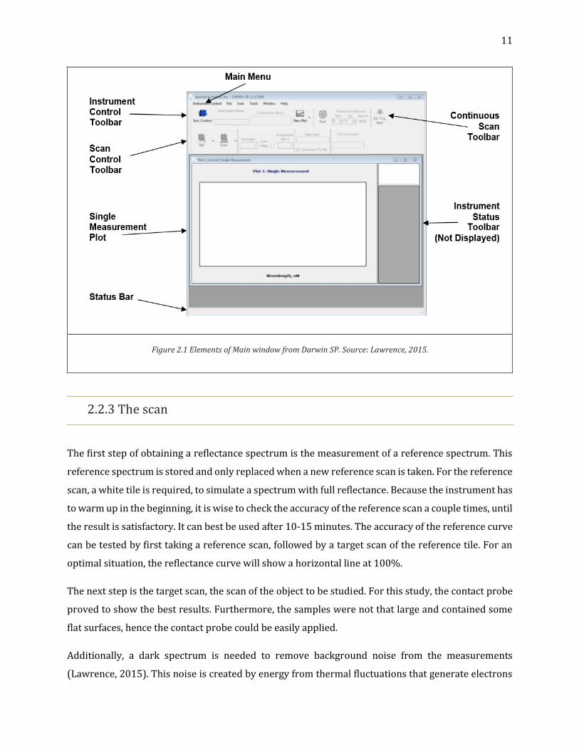
2.2.2 Main menu

In the main menu a new plot can be created, where the user can choose a single measurement plot or

a multiple measurement plot. The latter can be useful as different spectra can be directly compared.

This option was often chosen to compare the differences in spectra for the same rock sample. The plot

is shown below the main menu, where the wavelength (x-axis) is displayed in nm (figure 2.1). Next to

the plot window, on the right, instrument data and measured data is displayed after the target scan is

made. This data is directly stored under the name that was assigned in the instrument control panel,

if the “save scan data to file” option in the main menu is on. Other important functions displayed in

the main menu, are the reference and target scan, to measure the spectra. The continuous scan option

allows the user to measure the target with the contact probe, which is useful for rocks with irregular

surfaces. The “next scan” option, displayed in the main window, shows the name of the next scan that

is made, where it automatically summarizes the scan by number. Some tools are included, such as a

spectral library from the USGS (SpecLib V6) and some spectral vegetation indices, such as the

Normalized Vegetation Index (NDVI).

The “Avg scan time” function can be used to alter the number of scans, over which the average is

taken. A value between 1 and 100 can be chosen, where an increasing number of averages causes a

smoothening of noisy signals. However, with a higher average more time is needed to complete the

scan. In this study an Avg of 50 is used for measurements. The effect of this option to the results is

analysed, where a granite sample is measured with the Avg. time= 100 as a reference scan. Then

multiple measurements are taken with a Avg. time steps of 10, and the spectra are compared to the

reference scan of 100.

11

Figure 2.1 Elements of Main window from Darwin SP. Source: Lawrence, 2015.

2.2.3 The scan

The first step of obtaining a reflectance spectrum is the measurement of a reference spectrum. This

reference spectrum is stored and only replaced when a new reference scan is taken. For the reference

scan, a white tile is required, to simulate a spectrum with full reflectance. Because the instrument has

to warm up in the beginning, it is wise to check the accuracy of the reference scan a couple times, until

the result is satisfactory. It can best be used after 10-15 minutes. The accuracy of the reference curve

can be tested by first taking a reference scan, followed by a target scan of the reference tile. For an

optimal situation, the reflectance curve will show a horizontal line at 100%.

The next step is the target scan, the scan of the object to be studied. For this study, the contact probe

proved to show the best results. Furthermore, the samples were not that large and contained some

flat surfaces, hence the contact probe could be easily applied.

Additionally, a dark spectrum is needed to remove background noise from the measurements

(Lawrence, 2015). This noise is created by energy from thermal fluctuations that generate electrons

12

in the same way photons do (StellarNet, 2017). This noise is always present, even when light is not,

and increases with higher temperatures (StellarNet, 2017).The Dark Mode is done internally, where

a shutter automatically closes for a moment, right before the measurement is taken (Lawrence, 2015).

The dark data is recorded and used to refine the detector data from the spectral instrument.

In general, Automatic Dark Mode is more sufficient, as the user does not have to take frequent Dark

Mode measurements (Lawrence, 2015). A scaled Dark Mode becomes useful when timing becomes of

interest (high speed, external triggering, pulsed operation).

During the scan process, 3-5 scans were taken of each sample whenever possible. For a few samples,

only a single scan could be taken, due to their size or irregular surface. Every time a new sample was

measured, the reference scan was renewed. Before the first sample was measured and the instrument

had to warm up, a few reference scans were taken, to assure the accuracy of the instrument was

satisfactory, which was mostly after 10-15 minutes. After this, the instrument remained on during the

whole day of measuring. The light of the contact probe was sometimes turned off for a few minutes

when it was not in use, as the contact probe would heat up to high temperatures.

13

3 RESULTS

3.1 Spectral analysis of the Suriname Collection

3.1.1 Minerals

The spectral curves of hematite (TU Delft, 1918, figure 3.1-A) and gibbsite (van Kersen, 1955, figure

3.1-B) from the Suriname collection are plotted in graph 3.1, together with the hematite and gibbsite

curves of the USGS spectral library. Both hematite and gibbsite contain additional features compared

to spectral curves of the USGS. For gibbsite this is at 810-1245 nm and for hematite, additional

features occur between 743-1370 nm and 1880-2132 nm. When the measured gibbsite and hematite

are plotted together with the measured ferrite from the Waniwiro hills (van Kersen 1955), it becomes

clear that both samples contain impurities by iron.

The samples pyrolusite, pyrite and ferberite, from the collection of Brinck (1956), are plotted in the

same graph. Pictures of all three samples can be seen in figure 3.2. Pyrolusite is the most common

manganese mineral and ferberite is the iron-rich endmember of the mineral series wolframite, which

also contains variable amounts of manganese (Friedman, 1997-2017). Pyrite is a mineral composed

of ironsulfide. Graph 3.2 shows the pyrolusite sample is also rich in iron, presenting a very similar

curve to that of ferrite. The USGS spectral library also contains a spectral signature of pyrolusite,

which does not show any absorption features. The double absorption features of the ferberite sample

between 1370-1445 nm, 1880-2060 and 2128-2231 nm, coincide with the spectral curve of ferrite,

as do the absorption features between 1750-1230 nm, 1370-1445, 1880-2060 nm 2160-2236 nm

from the pyrite curve, confirming the presence of iron in both ferberite and pyrite samples.

14

A

B

Figure 3.1-A Hematite sample from Rorac, NE Suriname. Figure 3.1-B Gibbsite sample from Nassau Mountains, NE Suriname.

Gibbsite USGS

Gibbsite

(Nassau

Mountain)

Hematite (Rorac)

Hematite USGS

Wavelength (nm)

Re

fle

cta

nce

Wavelength (nm)

Re

fle

cta

nce

(ra

tio

)

Gibbsite

(Nassau

Mountain)

Hematite (Rorac)

Ferrite

Graph 3.1 A. Spectral curves of gibbsite and hematite, displayed in ENVI 5.2 and B. spectral curves of hematite and gibbsite compared to ferrite.

15

Ferberite

(de Jong Zuid)

Re

fle

cta

nce

(ra

tio

)

Ferrite

Wavelength (nm)

Pyrolusite USGS

Pyrolusite

(Haute Rufin)

Pyrite

(Lawa river)

Graph 3.2 Spectral signatures of pyrolusite, ferberite, pyrite and ferrite , displayed in ENVI 5.2

Figure 3.2 Samples of A. pyrite from Haute Rufin, B. pyrolusite from Haute Rufin and C. ferberite from Pakira Hill, de Jong

zuid. All locations are in East Suriname.

A B

C

16

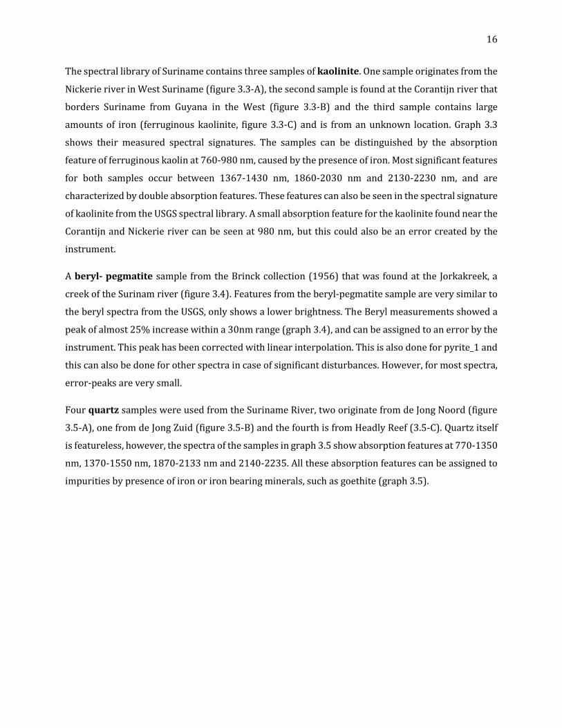
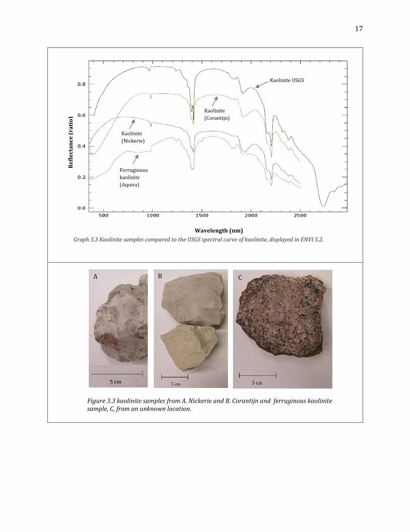
The spectral library of Suriname contains three samples of kaolinite. One sample originates from the

Nickerie river in West Suriname (figure 3.3-A), the second sample is found at the Corantijn river that

borders Suriname from Guyana in the West (figure 3.3-B) and the third sample contains large

amounts of iron (ferruginous kaolinite, figure 3.3-C) and is from an unknown location. Graph 3.3

shows their measured spectral signatures. The samples can be distinguished by the absorption

feature of ferruginous kaolin at 760-980 nm, caused by the presence of iron. Most significant features

for both samples occur between 1367-1430 nm, 1860-2030 nm and 2130-2230 nm, and are

characterized by double absorption features. These features can also be seen in the spectral signature

of kaolinite from the USGS spectral library. A small absorption feature for the kaolinite found near the

Corantijn and Nickerie river can be seen at 980 nm, but this could also be an error created by the

instrument.

A beryl- pegmatite sample from the Brinck collection (1956) that was found at the Jorkakreek, a

creek of the Surinam river (figure 3.4). Features from the beryl-pegmatite sample are very similar to

the beryl spectra from the USGS, only shows a lower brightness. The Beryl measurements showed a

peak of almost 25% increase within a 30nm range (graph 3.4), and can be assigned to an error by the

instrument. This peak has been corrected with linear interpolation. This is also done for pyrite_1 and

this can also be done for other spectra in case of significant disturbances. However, for most spectra,

error-peaks are very small.

Four quartz samples were used from the Suriname River, two originate from de Jong Noord (figure

3.5-A), one from de Jong Zuid (figure 3.5-B) and the fourth is from Headly Reef (3.5-C). Quartz itself

is featureless, however, the spectra of the samples in graph 3.5 show absorption features at 770-1350

nm, 1370-1550 nm, 1870-2133 nm and 2140-2235. All these absorption features can be assigned to

impurities by presence of iron or iron bearing minerals, such as goethite (graph 3.5).

17

Re

fle

cta

nce

(ra

tio

)

Kaolinite USGS

Kaolinite

(Corantijn)

Wavelength (nm)

Kaolinite

(Nickerie)

Ferruginous

kaolinite

(Aquira)

Graph 3.3 Kaolinite samples compared to the USGS spectral curve of kaolinite, displayed in ENVI 5.2.

Figure 3.3 kaolinite samples from A. Nickerie and B. Corantijn and ferruginous kaolinite sample, C, from an unknown location.

A B C

18

Figure 3.4 Beryl- pegmatite sample from Jorkakreek, Marowijne River.

Wavelength (nm)

Wavelength (nm)

Re

fle

cta

nce

R

efl

ect

an

ce

Graph 3.4 Beryl corrected with linear interpolation. Green spectrum is from USGS spectral library. Red and purple are measured and corrected measurement of beryl respectively.

19

Re

fle

cta

nce

(ra

tio

)

Ferrite

Quartz

(de Jong Noord)

Quartz

(de Jong Zuid)

Quartz

(Headly Reef)

Wavelength (nm)

Graph 3.5 Spectral signatures of quartz samples compared to ferrite, displayed in ENVI 5.2.

Figure 3.5-B Quartz sample from de Jong Zuid, NE Suriname.

Figure 3.5-A Quartz sample from de Jong Noord, NE Suriname

Figure 3.5-C Quartz sample from Headly Reef, Suriname River.

20

A few quartz samples that are included contain beforehand known impurities. A quartz-diorite

sample, quartz-gold sample and quartz-hematite sample are analysed. The samples can be seen in

figure 3.6 and their spectral curves are shown in graph 3.6. For the quartz-gold and quartz-hematite

samples the features can be attributed to the presence of iron. The mineral hematite does not contain

significant features and the spectral curve of gold is not known. The quartz-diorite sample contains

Graph 3.6 Spectral signatures of impure quartz samples compared, displayed in ENVI 5.2.

Re

fle

cta

nce

(ra

tio

)

Wavelength (nm)

Olioclase USGS

Quartz-hematite

Quartz-gold

Quartz-diorite

Figure 3.6 A. quartz-diorite sample, B. quartz-gold sample and C. quartz-hematite sample.

A B C

21

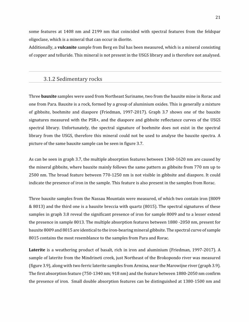
some features at 1408 nm and 2199 nm that coincided with spectral features from the feldspar

oligoclase, which is a mineral that can occur in diorite.

Additionally, a vulcanite sample from Berg en Dal has been measured, which is a mineral consisting

of copper and telluride. This mineral is not present in the USGS library and is therefore not analysed.

3.1.2 Sedimentary rocks

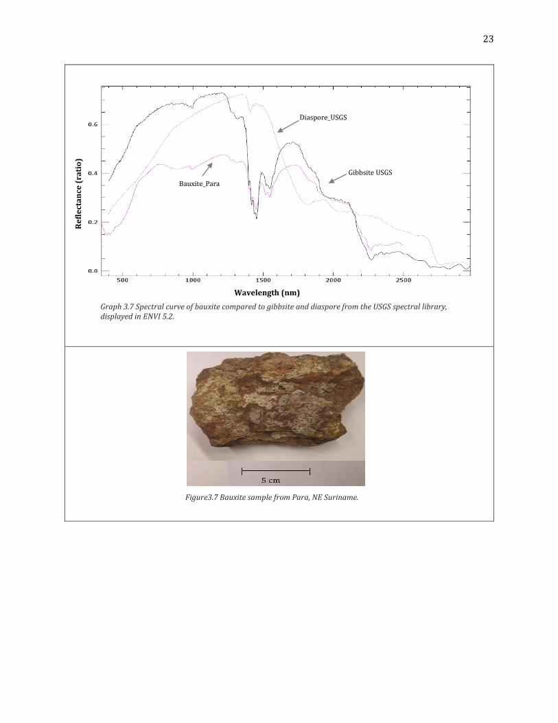
Three bauxite samples were used from Northeast Suriname, two from the bauxite mine in Rorac and

one from Para. Bauxite is a rock, formed by a group of aluminium oxides. This is generally a mixture

of gibbsite, boehmite and diaspore (Friedman, 1997-2017). Graph 3.7 shows one of the bauxite

signatures measured with the PSR+, and the diaspore and gibbsite reflectance curves of the USGS

spectral library. Unfortunately, the spectral signature of boehmite does not exist in the spectral

library from the USGS, therefore this mineral could not be used to analyse the bauxite spectra. A

picture of the same bauxite sample can be seen in figure 3.7.

As can be seen in graph 3.7, the multiple absorption features between 1360-1620 nm are caused by

the mineral gibbsite, where bauxite mainly follows the same pattern as gibbsite from 770 nm up to

2500 nm. The broad feature between 770-1250 nm is not visible in gibbsite and diaspore. It could

indicate the presence of iron in the sample. This feature is also present in the samples from Rorac.

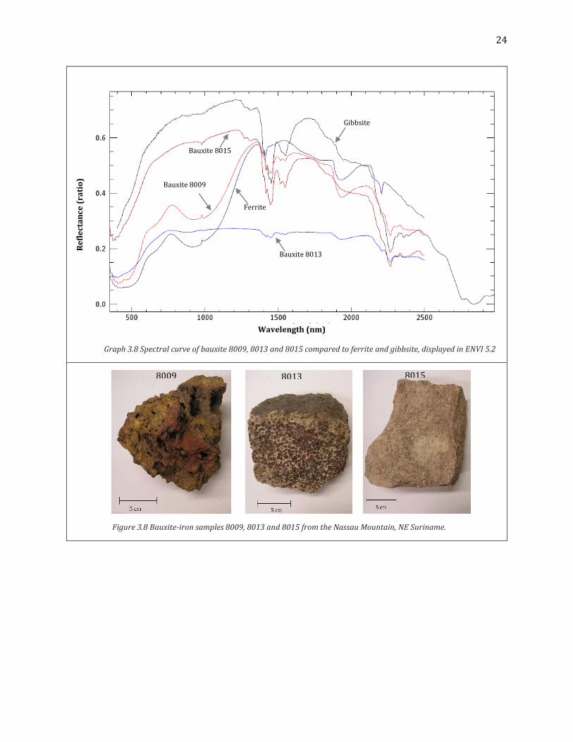
Three bauxite samples from the Nassau Mountain were measured, of which two contain iron (8009

& 8013) and the third one is a bauxite breccia with quartz (8015). The spectral signatures of these

samples in graph 3.8 reveal the significant presence of iron for sample 8009 and to a lesser extend

the presence in sample 8013. The multiple absorption features between 1880 -2050 nm, present for

bauxite 8009 and 8015 are identical to the iron-bearing mineral gibbsite. The spectral curve of sample

8015 contains the most resemblance to the samples from Para and Rorac.

Laterite is a weathering product of basalt, rich in iron and aluminium (Friedman, 1997-2017). A

sample of laterite from the Mindrineti creek, just Northeast of the Brokopondo river was measured

(figure 3.9), along with two ferric laterite samples from Armina, near the Marowijne river (graph 3.9).

The first absorption feature (750-1340 nm; 918 nm) and the feature between 1880-2050 nm confirm

the presence of iron. Small double absorption features can be distinguished at 1380-1500 nm and

22

one with its maximum depth at 2208 for all three samples. These features could be caused by various

minerals, such as: muscovite, illite, gibbsite, kaolinite or serpentine.

Conglomerate rocks consist of gravel-sized clasts, which are cemented together by calcite, silica or

iron-oxide (O’Connor, 2005). A conglomerate sample from the Kabalebo river in West Suriname was

measured (figure 3.10). Graph 3.10 shows the presence of iron and that calcite is most likely not

present for this sample.

Shale is a clay, consisting of quartz and feldspars. Feldspar is an aluminium silicate mineral

(Friedman, 1997-2017). The spectra of some feldspar minerals are shown in graph 3.11 together with

the measured shale spectra. Quartz minerals are featureless and so are most feldspar minerals in the

400-2500 nm wavelength part of the spectrum. The measured shale spectrum does not contain any

notable features, apart from a tiny one at 2209 nm. This feature is too small to be correlated to any

feldspar mineral. Small features at 980 and 1880 are measurement errors. The measured shale

sample is shown in figure 3.11.

23

Figure3.7 Bauxite sample from Para, NE Suriname.

Graph 3.7 Spectral curve of bauxite compared to gibbsite and diaspore from the USGS spectral library, displayed in ENVI 5.2.

Bauxite_Para

Gibbsite USGS

Diaspore_USGS

Re

fle

cta

nce

(ra

tio

)

Wavelength (nm)

24

Figure 3.8 Bauxite-iron samples 8009, 8013 and 8015 from the Nassau Mountain, NE Suriname.

8009 8013 8015

Graph 3.8 Spectral curve of bauxite 8009, 8013 and 8015 compared to ferrite and gibbsite, displayed in ENVI 5.2

Re

fle

cta

nce

(ra

tio

)

Wavelength (nm)

Ferrite

Bauxite 8013

Bauxite 8009

Gibbsite

Bauxite 8015

25

Figure 3.9 Laterite sample from Mindrinetti

Graph 3.9 Spectral curve of laterite and ferrite displayed in ENVI 5.2

Ferrite

Laterite

(Mindrinetti)

Laterite

(Marowijne)

Re

fle

cta

nce

(ra

tio

)

Wavelength (nm)

26

Figure 3.10 Conglomerate sample from Kabalebo river, West Suriname.

Re

fle

cta

nce

(ra

tio

)

Ferrite

Wavelength (nm)

Conglomerate (Kabalebo

river)

Calcite USGS

Graph 3.10 Spectral curve of conglomerate compared to ferrite and calcite, displayed in ENVI 5.2

27

.

Shale (Siparinikreek)

Anorthite USGS

Orthoclase USGS

Quartz USGS

Bytownite USGS

Labradorite USGS

Re

fle

cta

nce

(ra

tio

)

Wavelength (nm)

Graph 3.11 Spectral curve of Shale compared to feldspar minerals and quartz, displayed in ENVI 5.2

Figure 3.11 Shale sample from Marowijne river.

28

3.1.3 Metamorphic rocks

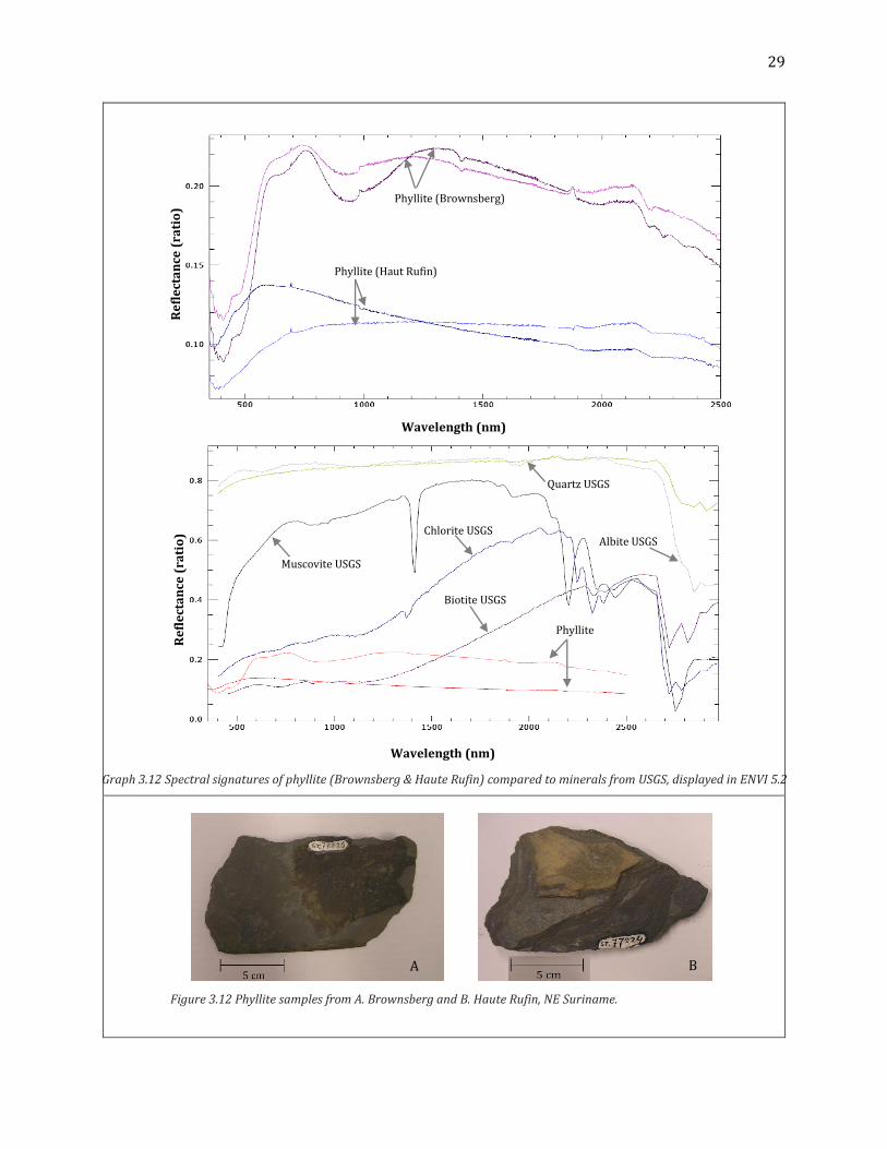
Phyllite samples were used from Brownsberg, near the Brokopondo lake (figure 3.12-A) and from

Haute Rufin, near the Lawa river (figure 3.12-B). Phyllite is a metamorphic rock, intermediate

between slate and schist, with shale as a parent rock (Wicander & Monroe, 2013). In general, all

curves shown in graph 3.12 are relatively featureless, because of the quartz minerals. The phyllite

that originated from Brownsberg shows an absorption feature between 780-1216 nm, with its

deepest point around 940 nm, which could indicate the presence of iron. The feature from either

chlorite or muscovite at 1410 is also present for the phyllite in Brownsberg, but not for the phyllite

found near Lawa river in Haute Rufin. All phyllite spectra show a small feature at 2200 nm, which

might be caused by the presence of iron. Peaks are visible at 694 for all measurements, most likely

another error from the instrument.

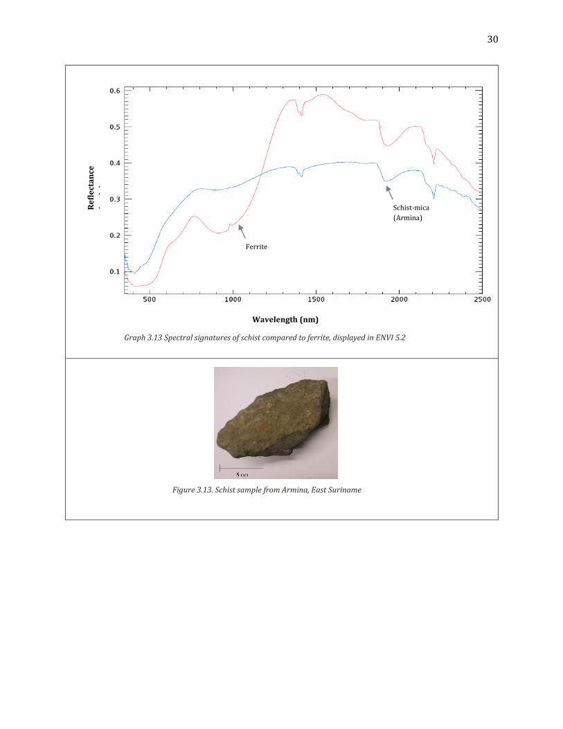
A schist-mica sample was measured from Armina, near Marowijne river (graph 3.13, figure 3.13).

Unlike the spectral signatures from shale and phyllite, the schist-mica contains various absorption

features. When the curve is plotted along with ferrite, it can be clearly seen that these features are

caused by iron.

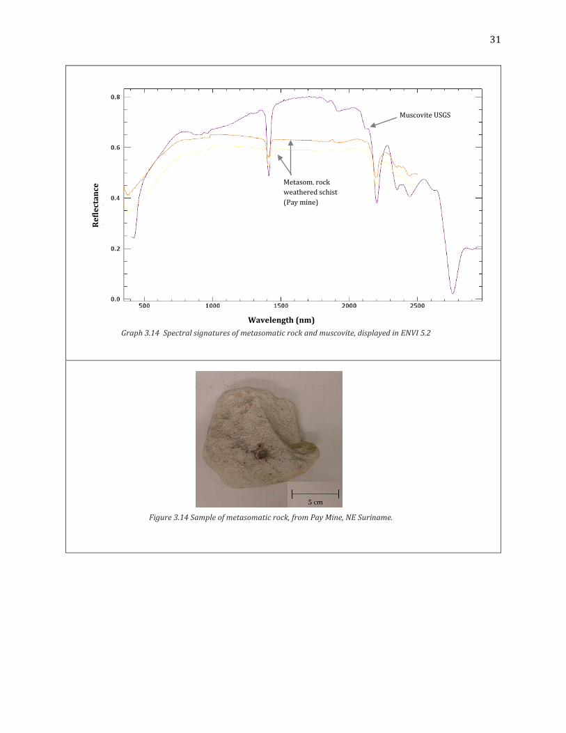
A sample of metasomatic rock of weathered schist was used from the Pay mine in Rosebel (Brinck,

1956). Metasomatic is a metamorphic process where alteration of the chemical composition of the

rock takes place (Zharikov et al., 2007). The spectral signatures in graph 3.14 shows a strong presence

of muscovite. The sample can be seen in figure 3.14.

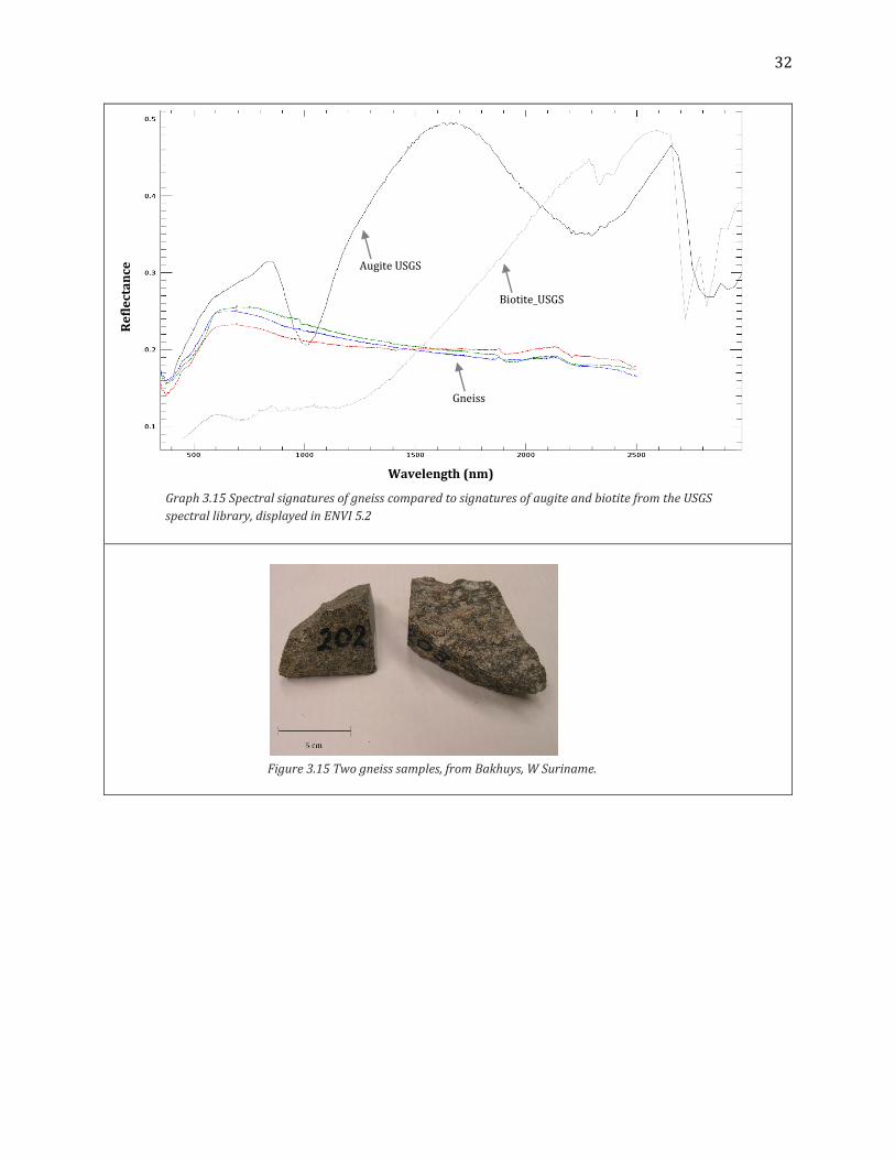
Gneiss is formed by metamorphosis of schist under high-grade conditions. Its reflectance curve is

similar to that of phyllite, as they share the parent rock shale (figure 1.2). Two gneiss samples were

measured from the Bakhuys expedition in Kabalebo, West Suriname (figure 3.15). The spectral curves

of the samples shown in graph 3.15 are nearly featureless in the 400-2500 nm range, except for the

optical range. A small feature at 2300 nm can be caused by biotite. Augite is also a common mineral

in gneiss (O’Connor, 2005). However, features of these spectra cannot be traced back in the measured

reflectance curves of these gneiss samples. The features at 980 and 1880 are probably caused by the

error of the detectors.

29

Graph 3.12 Spectral signatures of phyllite (Brownsberg & Haute Rufin) compared to minerals from USGS, displayed in ENVI 5.2

Figure 3.12 Phyllite samples from A. Brownsberg and B. Haute Rufin, NE Suriname.

A B

Wavelength (nm)

Re

fle

cta

nce

(ra

tio

) R

efl

ect

an

ce (

rati

o)

Wavelength (nm)

Phyllite (Haut Rufin)

Phyllite (Brownsberg)

Quartz USGS

Albite USGS

Muscovite USGS

Chlorite USGS

Biotite USGS

Phyllite

30

Re

fle

cta

nce

(ra

tio

)

Ferrite

Wavelength (nm)

Schist-mica

(Armina)

Graph 3.13 Spectral signatures of schist compared to ferrite, displayed in ENVI 5.2

Figure 3.13. Schist sample from Armina, East Suriname

31

Wavelength (nm)

Re

fle

cta

nce

(ra

tio

) Muscovite USGS

Metasom. rock

weathered schist

(Pay mine)

Graph 3.14 Spectral signatures of metasomatic rock and muscovite, displayed in ENVI 5.2

Figure 3.14 Sample of metasomatic rock, from Pay Mine, NE Suriname.

32

Wavelength (nm)

Re

fle

cta

nce

(ra

tio

)

Gneiss

Augite USGS

Biotite_USGS

Graph 3.15 Spectral signatures of gneiss compared to signatures of augite and biotite from the USGS

spectral library, displayed in ENVI 5.2

Figure 3.15 Two gneiss samples, from Bakhuys, W Suriname.

33

A greenstone sample from the van Kersen (1955) collection is used, that originates from the Nassau

Mountain (figure 3.16). Greenstone describes metamorphic rocks formed under low pressures and

temperatures, containing green minerals such as chlorite, serpentine or epidote (Friedman, 1997-

2017). The spectra of these minerals are plotted together with the one of the greenstone sample,

which contains a small feature at 1404 nm, 2015 and 2054 nm and 2345 nm (graph 3.16). The

position of most of these features coincides with the spectral curve of epidote. The feature at 2015

nm can be caused by the mineral serpentine. Features of chlorite are not found in the curve from the

greenstone sample from Nassau Mountain, which indicates a lack of its presence.

A hornfels sample from Nassau Mountain was measured (van Kersen, 1955; figure 3.17). Hornfels

are rocks derived from argillaceous sandstones, such as shale (Lay, 2009). The mineral composition

of hornfels is dependent on the parent rock, but mostly contains minerals that are formed under high

temperature conditions, such as coredierite and andalusite. Graph 3.17 shows that the hornfels

sample contains iron (780-1350 nm, 1860-2050 nm, 1413 nm). The absorption features at 2255 nm

and 7161 nm cannot be correlated to the features from the mineral coredierite or andalusite, but do

coincide with the features of the greenstone sample at the same wavelengths. This could indicate the

presence of epidote for this sample as well. The green colour of the hornfels sample reinforces this

possibility.

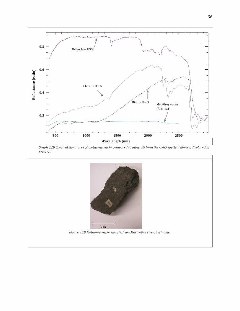
The Metagreywacke sample from the Marowijne river, Armina is nearly featureless, as it contains

quartz minerals (O’Connor, 2005)(graph 3.18; figure 3.18). A tiny feature at 1407 nm could be caused

by the feldspar mineral orthoclase. Small features at 2250 nm and 2340 nm indicate small presences

of chlorite and biotite minerals.

34

Figure 3.16 Greenstone sample, from Nassau Mountain, NE Suriname.

Wavelength (nm)

Re

fle

cta

nce

(ra

tio

)

Serpentine USGS

Greenstone

(Nassau Mountain)

Epidote USGS

Chlorite USGS

Graph 3.16 Spectral signatures of gneiss compared to signatures of augite and biotite from the USGS

spectral library, displayed in ENVI 5.2

35

Wavelength (nm)

Re

fle

cta

nce

(ra

tio

)

Coredierite USGS

Andalusite USGS

Ferrite

Chlorite USGS

Hornfels

(Nassau Mountain)

Graph 3.17 Spectral signature of hornfels compared to minerals from the USGS spectral library, displayed in

ENVI 5.2

Figure 3.17 Hornfels sample from Nassau Mountain, NE Suriname.

36

Wavelength (nm)

Re

fle

cta

nce

(ra

tio

)

Orthoclase USGS

Chlorite USGS

Biotite USGS MetaGreywacke

(Armina)

Graph 3.18 Spectral signatures of metagraywacke compared to minerals from the USGS spectral library, displayed in

ENVI 5.2

Figure 3.18 Metagreywacke sample, from Marowijne river, Suriname.

37

3.1.4 Igneous rocks

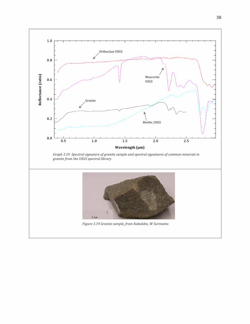
Granite consists mostly of orthoclase, Plagioclase and quartz. Orthoclase and Plagioclase are

featureless in the 700-2500 nm range of the spectrum, causing Granite to be nearly featureless as

well. Small absorption features are caused by muscovite (1415 nm, 2350-2390 nm) and maybe biotite

(2300-2390 nm) (graph 3.19, figure 3.19).

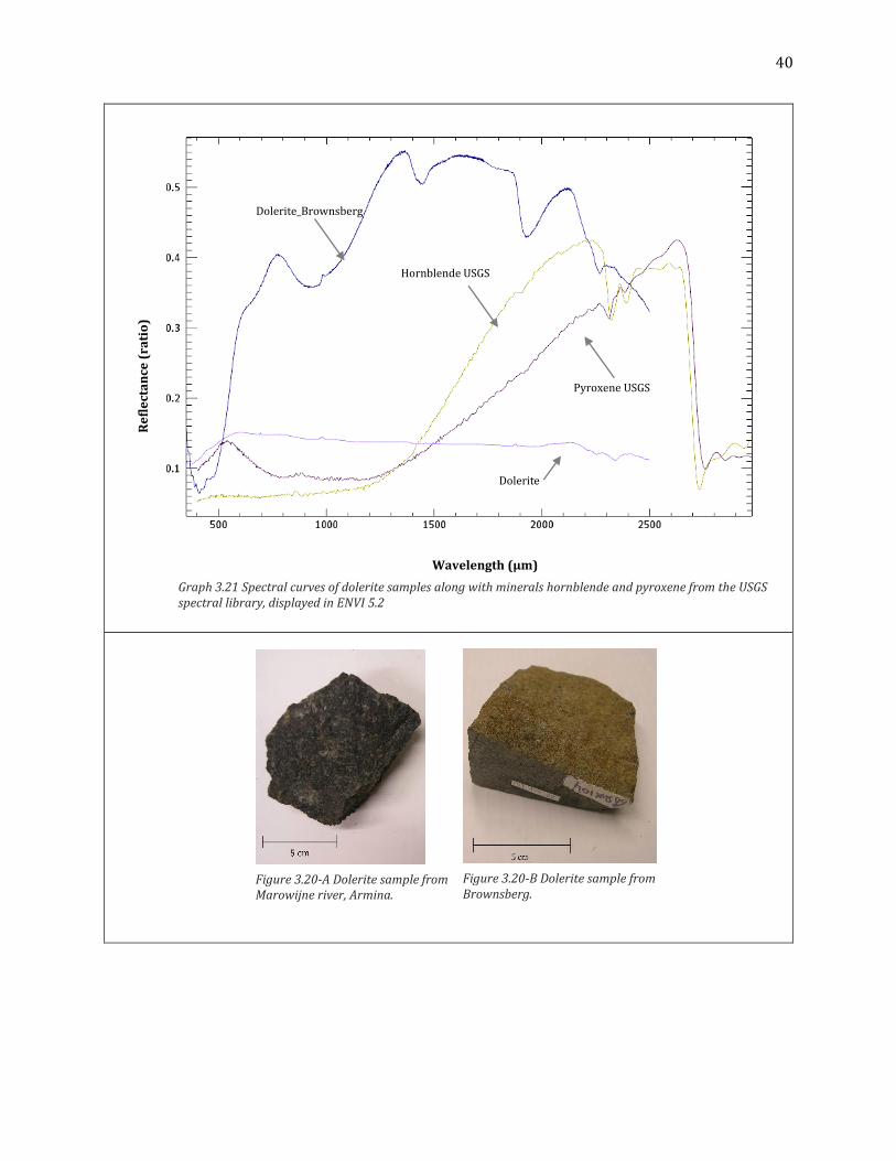
Multiple dolerite samples were measured from various locations (Armina; figure 3.20-A, Brownsweg;

figure 3.20-B). The reflectance curves from dolerite or diabase presented in graph 3.20 show a

variety in brightness, where most reflectance spectra remained below 0.2, but some exceeded 0.5.

Features occurred in the ranges of 780-1280 nm (960 nm), 1370-1585 (1415) nm and 1870- 2110

nm and can be assigned to the presence of iron, or iron-bearing minerals such as goethite. The spectra

that contain iron are from samples of Brownsweg. Most spectra contained barely any features.

Essential minerals of dolerite are plagioclase and pyroxene, and some non-essential minerals are K-

fledspar, hornblende and quartz (Mindat., n.d.). Unfortunately, plagioclase is not available in the USGS

spectral library, but graph 3.21 shows two dolerite spectral curves, together with a pyroxene and

hornblende spectral curve from the USGS library. However, features of the dolerite samples cannot

be linked to these minerals.

38

Wavelength (µm)

Re

fle

cta

nce

(ra

tio

)

Granite

Muscovite

USGS

Biotite_USGS

Orthoclase USGS

Graph 3.19 Spectral signature of granite sample and spectral signatures of common minerals in granite from the USGS spectral library

Figure 3.19 Granite sample, from Kabalebo, W Suriname.

39

Wavelength (µm)

Re

fle

cta

nce

(ra

tio

)

Graph 3.20 Spectral curves of dolerite samples displayed in ENVI 5.2

40

Dolerite_Brownsberg

Pyroxene USGS

Hornblende USGS

Dolerite

Wavelength (µm)

Re

fle

cta

nce

(ra

tio

)

Graph 3.21 Spectral curves of dolerite samples along with minerals hornblende and pyroxene from the USGS spectral library, displayed in ENVI 5.2

Figure 3.20-B Dolerite sample from Brownsberg.

Figure 3.20-A Dolerite sample from Marowijne river, Armina.

41

3.2 Analysis of the spectroradiometer PSR+3500

3.2.1 Accuracy instrument

Graph 3.22 shows the reference spectrum that was measured with the spectralon SRT-99-100 from

Labsphere. It can be seen clearly that there is a through- effect created by the transition of the

different detectors. Furthermore, the first detector shows a pattern consisting of peaks and

troughs/valleys deviating from the smooth curves of detectors two and three.

To test the accuracy of the instrument some target measurements of the spectralon have to be taken.

Graph 3.23 shows the ratio of a reference and target scan from the white tile after several minutes. A

line at 100% would indicate an error of 0%. The abrupt transition of the detectors is again visible,

creating a difference of 0.2%. It also shows that the second detector contains the least noise, which is

more present in detector three. Variations in the first detector are mainly caused by offset differences,

which results in a variation between 0.2% to 0.6%. It should be noted that even when the instrument

has warmed up, the accuracy varies with new measurements. After 10-15 minutes the instrument

was on, the average reflectance error from the detectors was in the range of 0.4-1.0%. The noise is

the most significant at the beginning and end of the wavelength spectrum.

Another pattern was observed, namely after the instrument has warmed up and the error seemed

relatively low (error<0.6%), the error increased after increasing the number of scans, without

renewing the reference scan (0.7%< error <1.0%). This while the contact probe was placed on the

D1 D2 D3

Graph 3.22 Spectral radiance curve of the spectralon reference tile (100%reflectance) in DARWin, where parts of the spectrum belonging to detectors 1, 2 and 3 are indicated.

42

spectralon and not touched during the measurements. It proves that to reduce the error of the

measurements, it is important to regularly refresh the reference scan.

3.2.2 Effect accuracy on measurements

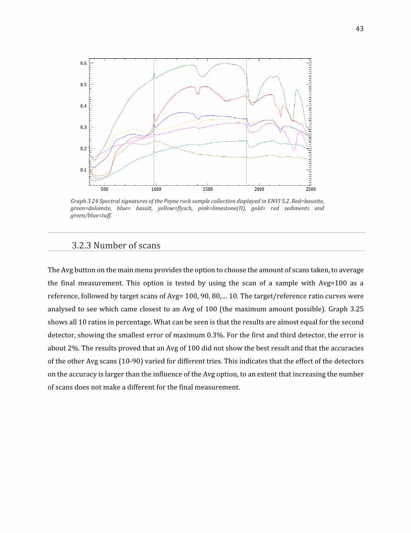
Graph 3.24 shows the reflectance spectra of multiple samples from the Peyne collection, measured

with the contact probe. In general the curves of the same sample show the same pattern but variate

in height due to differences in brightness of the sample. In the optical range 350-650 nm, the

reflectance curve shows a rippling pattern, similar to the curve of the reference spectrum in graph

3.22. However, for each target measurement this pattern, or the magnitude of the peaks and throughs

of the pattern, deviates from the pattern of the reference scan, allowing it to be visible in the

reflectance curve as well.

Furthermore, due to the transition of detectors, peaks are created at certain wavelengths. For every

measurement, a peak is present at around 980 nm and a smaller peak at 1880 nm. An additional peak

can sometimes be seen at 690 nm. The severity of the peaks varies for different measurements. It

might help to renew the reference measurement more often, however the peaks will always be visible.

Graph 3.23 Ratio of reference and target measurement of white tile.

43

3.2.3 Number of scans

The Avg button on the main menu provides the option to choose the amount of scans taken, to average

the final measurement. This option is tested by using the scan of a sample with Avg=100 as a

reference, followed by target scans of Avg= 100, 90, 80,… 10. The target/reference ratio curves were

analysed to see which came closest to an Avg of 100 (the maximum amount possible). Graph 3.25

shows all 10 ratios in percentage. What can be seen is that the results are almost equal for the second

detector, showing the smallest error of maximum 0.3%. For the first and third detector, the error is

about 2%. The results proved that an Avg of 100 did not show the best result and that the accuracies

of the other Avg scans (10-90) varied for different tries. This indicates that the effect of the detectors

on the accuracy is larger than the influence of the Avg option, to an extent that increasing the number

of scans does not make a different for the final measurement.

Graph 3.24 Spectral signatures of the Peyne rock sample collection displayed in ENVI 5.2. Red=bauxite, green=dolomite, blue= basalt, yellow=flysch, pink=limestone(II), gold= red sediments and green/blue=tuff.

44

3.2.4 Contact probe

The measurements of the contact probe can be influenced in multiple ways by both the sample and

the user. Three of these manners were tested and it was studied in which way they affect the spectral

measurements.

Surface irregularities

The rock samples of both collections show a large variety in shape. For some samples, flat surfaces

are difficult to find. With a bauxite sample from the Peyne collection, two scans are taken. The first

scan is taken with the contact probe placed on the rock sample, but for the second scan the contact

probe is only partially placed on the sample.

Graph 3.25 Ratio of Avg number (total number of scans of which an average is taken for the final measurement) over the Avg of 100.

45

The resulting spectral signatures of both measurements can be seen in graph 3.26. It shows that for

the reflectance curve where the contact probe is not correctly placed on the sample, the spectral

signature is lower in reflectance, but the shape and features of the curve remains the same. This

indicates that there is no interference of the lightning (fluorescent) with the measurement.

Because mostly the Suriname collection contains some samples with very irregular surfaces, this test

is also done for gibbsite, but now the contact probe is placed on a relatively flat part of the sample

during the first scan and placed on an irregular part of the surface for the second scan. The resulting

curves show the same decrease in reflectance and also show no difference in the shape.

Smooth surfaces

There are also samples that contain a relatively flat surface, which makes it possible to place the

contact probe on the sample instead of holding it. In this way, the contact probe will remain still

during all the scans over which it averages. The noise of holding the sample by hand was tested with

flysch from the Peyne collection. A scan of the flysch sample was used as a reference scan. The contact

probe is released from the sample and placed on the sample at the approximately same position for

the target scan. For the second target scan, the contact probe was picked up again and held against

the sample. A third scan was made where both the probe and the sample were held. Measurements

are repeated once or twice.

Graph 3.26 Spectral reflectance curves of bauxite from the Peyne collection, displayed in DARWin. Dark blue= rock sample completely covers the contact probe lense during scan measurement, light blue=contact probe is only partially placed on scan.

46

Graph 3.27 shows that when the contact probe is held by hand, the reflectance curve is higher, but

also show that the noise is not necessarily larger. The smallest error was actually measured when

both the contact probe and sample were held by hand (± by 3%).

Graph 3.27 Spectral reflectance curves of flysch. Blue= contact probe placed on sample, not touched during measurement, orange= contact probe held by hand, green=sample & contact probe held by hand.

47

4 DISCUSSION

A study of the Rosebel mine, held by Carlier (2012), revealed that the mineralogy of that area was

dominated by three mineral groups: Kaolinites, white mica’s (muscovite, paragonite) and chlorites

(Fe- chlorites). In this study, many rocks contained iron or iron-bearing minerals, which could be the

same Fe- chlorites. Muscovite minerals were also present in multiple samples. For the greenstone and

hornfels sample, chlorite minerals did not appear to be present, but instead it seemed that most

features were caused by the mineral epidote.

This spectral library was created as an aid for remote sensing image interpretation for images of

Suriname. However, geological image interpretation of Suriname is not an easy task. Apart from some

interferences by clouds, the incredible amount of vegetation that covers the country could make it

very difficult to identify mineralogy of Suriname. Locations of (old) mining areas are nearly the only

bare spots available for geological image interpretation, but these rocks are mostly weathered due to

protracted exposure. It should also be noted that the proportions of the mineral compositions vary

for the same rock types at different locations, or even at the same location, which makes it difficult to

assign one spectral reflectance curve to a specific rock.

Concerning the evaluation of the PSR+ spectroradiometer, it appeared that the first detector caused

the most deviations in the spectral curves measurements, due to differences in offset of the curves.

This detector is a different kind of detector (512 element Si photodiode array) than the second and

third detectors, which are both of the same type (256 element extended InGaAs photodiode array).

However, the second and third detector also showed a difference in accuracy, where the third

detector caused significantly more noise. To improve the spectral reflectance curves, which is mostly

needed for the optical range in the spectrum (first detector), the noise, difference in offset and the

transition in detectors should be as small as possible.

Analysis of the PSR+ showed peaks at transitions of detectors on the wavelength spectrum. The

severity of these peaks varied for different measurements. So far, no correlation between the

instrument temperature and increase in peak errors has been found, but this is not thoroughly

studied. Refreshing the reference scan more often might decrease the severity of the peak. The exact

cause that increases the error should be further studied.

48

5 CONCLUSION

This research about the spectral reflectance curves of samples from Suriname, which were measured

with the recently purchased PSR+3500 spectrometer, consisted of two research objectives.

Creating a spectral library from a rock collection of Naturalis, for minerals that are of

importance to the Greenstone Belt formation and analyse the spectral differences between

these minerals.

A spectral library was created with the PSR+ spectrometer and analysed. The minerals in the selection

showed impurities by iron (gibbsite, hematite, quartz). For the minerals pyrolusite, pyrite and

ferberite, iron is a composite element, so these features could already be expected. Samples from the

metamorphic section mainly consisted of intermediate- to high-grade metamorphosed shale

(phyllite, schist, gneiss) and also for these rocks, except for gneiss, the most significant absorption

features were caused by iron. The spectral signatures of the metasomatic rock sample showed the

significant presence of the mineral muscovite and it appeared that the hornfels sample contained the

same green epidote mineral as the greenstone sample.

Testing the spectrometer PSR+ of the University of Utrecht with different rock fragments from

La Peyne, France.

Overall, the PSR+3500 showed relatively good results, especially for the NIR-SWIR region. This was

because the second detector contains the least amount of noise. The first detector showed the most

variations, caused by offset differences and the third detector showed more noise than the second. In

the optical region, the rippling pattern that was observed influences the spectral reflectance of the

measurements. Peaks were visible in the spectral curves at the wavelength range of the transition of

the detectors. The severity of these peaks differed for different measurements.

Results showed that the reference scan of the spectralon should be regularly refreshed, as noise

increases with increased amount of target scans. Furthermore, increasing the number of scans taken

to average each measurement in the Avg option, does not yield in better reflectance curves, as the

noise from the detectors is too large.

49

6 REFERENCES

Backwell, C.A., Bijkerk, C.G.J. (2010). An analysis of flash floods in the Peyne catchment southern

France, UU scriptiearchief.

Briegel, F.(2012). Country report of Suriname, Economic Research Department, Rabobank Nederland.

Brinck, J. W. (1956). Goudafzettingen in Suriname (Gold deposits in Surinam). Leidse Geologische

Mededelingen, 21(1), 1-246.

Carlier, L.C.F. (2012). Characterization of the geological and geo-chemical footprint of the Koolhoven

gold deposit, Suriname.

Friedman, H. (1997-2017). Minerals.net: the mineral and gemstone kingdom, consulted during 06-17

and 07-17, from: http://www.minerals.net/

Gibbs, A. K., & Olszewski, W. J. (1982). Zircon U Pb ages of Guyana greenstone-gneiss terrane.

Precambrian Research, 17(3-4), 199-214.

Haalboom, B. (2012). The intersection of corporate social responsibility guidelines and indigenous

rights: Examining neoliberal governance of a proposed mining project in Suriname. Geoforum, 43(5),

969-979.

De Jong, S. M., Pebesma, E. J., & Lacaze, B. (2003). Above‐ground biomass assessment of

Mediterranean forests using airborne imaging spectrometry: the DAIS Peyne experiment.

International Journal of Remote Sensing, 24(7), 1505-1520.

Kroonenberg, S.B. & Melitz , P.J. (1983). Summit levels, bedrock control and the etchplain concept in

the basement of Surinam, Geologie en Mijnbouw,62, 389-399.

Lawrence (2015). Spectral evolution: DARWin application software version 1.3 user manual. USA.

Lay, M.G.(2009). Metamorphosed rocks. In Handbook of road technology (fourth edition)

van der Meer, F.D. & de Jong, S.M. (2006) Imaging spectrometry; basic principles and prospective

applications, Springer, Dordrecht: the Netherlands.

Mindat. (n.d.). Mindat, consulted during 06-17 and -7-17, from: https://www.mindat.org/min-

48432.html

Mobbs. P.M.(2016). The mineral industries of Suriname, U.S. Geological Survey Minerals Yearbook

2013.

O’Connor. (2005). Rocks and minerals, consulted during 06-17 and 07-17, from:

https://flexiblelearning.auckland.ac.nz/rocks_minerals/rocks/

Spectral Evolution. (2012). PSR+ High resolution field portable spectroradiometer. Lawrence, USA.

50

Stellarnet. (2017). Stellarnet: what is a dark spectrum, consulted in 06-17From:

http://www.stellarnet.us/dark-spectrum-spectrawiz/

De Vletter, D. R., Aleva, G. J. J., & Kroonenberg, S. B. (1998). Research into the Precambrian of

Suriname. The history of earth sciences in Suriname. Royal Netherlands Academy of Science,

Netherlands Institute of Applied Geosciences, 15-63.

Wicander, R. & Monroe, J.S. (2013). Metamorphism and metamorphic rocks. In GEOL (2nd edition)

(pp.191). West Yorkshire: Brooks/Cole.