spectral analysis of the continuous and discretized heat and
TRANSCRIPT

Spectral analysis of the continuous and discretizedheat and advection equation on single and multiple
domains
Jens Lindstrom? and Jan Nordstrom??
?Uppsala University, Department of Information Technology, SE-751 05, Uppsala,Sweden, [email protected]
??Linkoping University, Department of Mathematics, SE-581 83, Linkoping,Sweden, [email protected]
Abstract
In this paper we study the heat and advection equation in single and mul-tiple domains. We discretize using a second order accurate finite differencemethod on Summation-By-Parts form with weak boundary and interface con-ditions. We derive analytic expressions for the spectrum of the continuousproblem and for their corresponding discretization matrices. We show howthe spectrum of the single domain operator is contained in the multi domainoperator spectrum when artificial interfaces are introduced. We study theimpact on the spectrum and discretization errors depending on the interfacetreatment and verify that the results are carried over to higher order accurateschemes.
1 Introduction
When solving partial differential equations (PDEs) as for example the Navier-Stokesequations, there is often a need to divide the computational domain into several sub-domains to allow for flexible geometry handling and sufficient resolution. The sub-domains need to be coupled in a way that preserves both the stability and accuracyof the computational scheme. A proof of stability and conservation for a multi-block method for the compressible Navier-Stokes equations was shown recently in[1]. They used a finite difference method on Summation-By-Parts (SBP) form withthe Simultaneous Approximation Term (SAT) technique to impose the boundaryand interface conditions weakly. The SBP and SAT method has been used for manyapplications in fluid dynamics since it has the benefit of being provable energy sta-ble when the correct boundary and interface conditions are imposed for the PDE[1, 2, 3, 4, 5, 6].
In this paper we investigate the details of the diffusion and advection operators byconsidering the one-dimensional heat and advection equation on single and multipledomains. The boundary and interface conditions are imposed weakly using the
1

SAT technique and the equations are discretized using a second order accurate SBPoperator. There are SBP operators of order 2, 3, 4 and 5 derived in for example[7, 8] and we stress that the stability analysis given in this paper holds for any orderof accuracy. The second order operators was chosen since it allows us to deriveanalytical results regarding certain spectral properties of the operators.
The reason for doing such an investigation is because the SBP operators areby construction one-sided at boundaries and interfaces. The weak implementationof the boundary and interface conditions significantly modifies the scheme close tothese points and we want to see exactly what influence these modifications have.
2 Single domain spectral analysis of the heat equa-
tion
In order to compare the effects on the spectrum when introducing an artificial in-terface we shall begin by decomposing the heat equation on a single domain bothcontinuously and discretized. This allows us to isolate expressions stemming fromthe boundaries only and separate them from the interface part.
2.1 Continuous case
Consider the heat equation on −1 ≤ x ≤ 1,
ut = uxx
u(x, 0) = f(x)
u(−1, t) = g1(t)
u(1, t) = g2(t).
(1)
To analyze (1) we introduce the Laplace transform
u = Lu =
∞∫0
e−studt (2)
which is defined for locally integrable functions on [0,∞) where the real part of shas to be sufficiently large. The basic property that we are going to use is that ittransform differentiation with respect to the time variable to multiplication with thecomplex number s. Hence a time-dependent PDE in Laplace transformed space isan ordinary differential equation (ODE) which we can solve. Finding analyticallythe inverse transformation is in general a very difficult problem but that is not ourinterest here.
We shall use the Laplace transform to determine the spectrum of (1). Assumethat g1 = g2 = 0 and take the Laplace transform of (1). The initial conditionis omitted since it does not enter in the spectral analysis. We get an ODE intransformed space,
su = uxx
u(−1, s) = 0
u(1, s) = 0,
(3)
2

which is an eigenvalue problem for s. By the ansatz u = ekx we can determine thatthe general solution to (3) is
u = c1e√sx + c2e
−√sx. (4)
By applying the boundary conditions we obtain
c1e−√s + c2e
√s = 0 (5)
c1e√s + c2e
−√s = 0 (6)
which we write in matrix form as[e−√s e
√s
e√s e−
√s
]︸ ︷︷ ︸
E(s)
[c1c2
]=
[00
]. (7)
Equation (7) will have a non-trivial solution when the coefficient matrix E(s) issingular. We hence seek the values of s such that the determinant is zero. We have
det(E(s)) = −2 sinh(2√s) (8)
which is zero for
s = −π2n2
4, n ∈ N. (9)
This infinite sequence of values is thus the spectrum of (1). Note that s = 0 is notconsidered a solution since then we have a double root and u = c1 + c2x. From theboundary conditions we get that u ≡ 0 and hence u ≡ 0, which is trivial.
Remark 2.1. Note that the spectrum is identical to that obtained by standard Sturm-Liouville theory but with the sign reversed. From the Gustafsson-Kreiss-Sundstromtheory point of view, the negative sign implies that (1) is well-posed [9].
2.2 Discrete case
To discretize (1) we use a second order accurate finite difference operator on SBPform,
uxx ≈ D2v (10)
where v = [v0, v1, . . . , vN ]T is the discrete grid function and the mesh is uniformwith N + 1 grid points. The exact form of the operator D2 is, see [7, 10],
D2 = P−1(−A+BD) =1
∆x2
0 0 0 0 · · · 01 −2 1 0 · · · 0...
. . . . . . . . . . . ....
0 · · · 0 1 −2 10 0 0 0 · · · 0
(11)
3
where
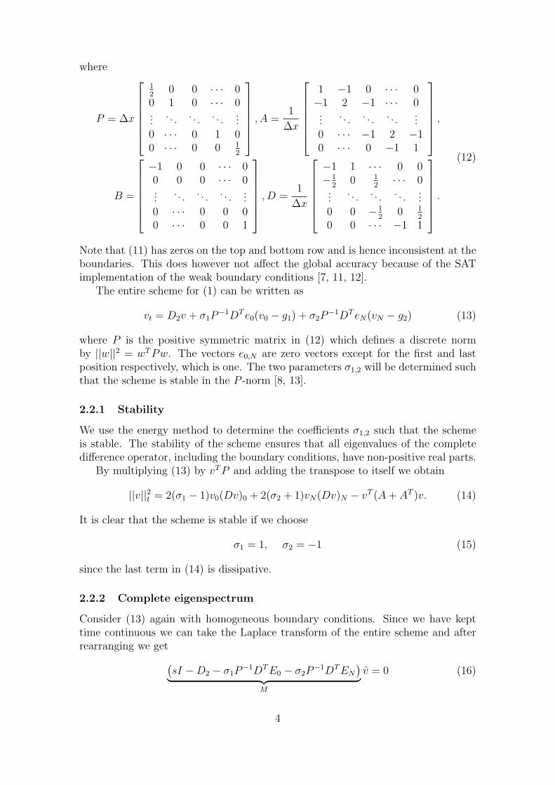
P = ∆x
12
0 0 · · · 00 1 0 · · · 0...
. . . . . . . . ....
0 · · · 0 1 00 · · · 0 0 1
2
, A =1
∆x
1 −1 0 · · · 0−1 2 −1 · · · 0...
. . . . . . . . ....
0 · · · −1 2 −10 · · · 0 −1 1
,
B =
−1 0 0 · · · 00 0 0 · · · 0...
. . . . . . . . ....
0 · · · 0 0 00 · · · 0 0 1
, D =1
∆x
−1 1 · · · 0 0−1
20 1
2· · · 0
.... . . . . . . . .
...0 0 −1
20 1
2
0 0 · · · −1 1
.(12)
Note that (11) has zeros on the top and bottom row and is hence inconsistent at theboundaries. This does however not affect the global accuracy because of the SATimplementation of the weak boundary conditions [7, 11, 12].
The entire scheme for (1) can be written as
vt = D2v + σ1P−1DT e0(v0 − g1) + σ2P
−1DT eN(vN − g2) (13)
where P is the positive symmetric matrix in (12) which defines a discrete normby ||w||2 = wTPw. The vectors e0,N are zero vectors except for the first and lastposition respectively, which is one. The two parameters σ1,2 will be determined suchthat the scheme is stable in the P -norm [8, 13].
2.2.1 Stability
We use the energy method to determine the coefficients σ1,2 such that the schemeis stable. The stability of the scheme ensures that all eigenvalues of the completedifference operator, including the boundary conditions, have non-positive real parts.
By multiplying (13) by vTP and adding the transpose to itself we obtain
||v||2t = 2(σ1 − 1)v0(Dv)0 + 2(σ2 + 1)vN(Dv)N − vT (A+ AT )v. (14)
It is clear that the scheme is stable if we choose
σ1 = 1, σ2 = −1 (15)
since the last term in (14) is dissipative.
2.2.2 Complete eigenspectrum
Consider (13) again with homogeneous boundary conditions. Since we have kepttime continuous we can take the Laplace transform of the entire scheme and afterrearranging we get(
sI −D2 − σ1P−1DTE0 − σ2P
−1DTEN)︸ ︷︷ ︸
M
v = 0 (16)
4

where I is the N + 1 dimensional identity operator and E0,N are zero matricesexcept for the (0, 0) and (N,N) positions respectively which is one. To determinethe complete eigenspectrum of the discrete operator M we start by considering thedifference scheme for an internal point. The internal scheme is the standard centralfinite difference scheme and hence
∂
∂tvi =
vi−1 − 2vi + vi+1
∆x2. (17)
By taking the Laplace transform of (17) we obtain a recurrence relation
svi =vi−1 − 2vi + vi+1
∆x2(18)
for which we can obtain the general solution by the ansatz vi = σκi. The ansatzyields the second order equation
κ2 − (s+ 2)κ+ 1 = 0 (19)
with the two solutions
κ+,− =s+ 2
2±
√(s+ 2
2
)2
− 1 (20)
where s = s∆x2. Hence the general solution to (18) is
vi = c1κi+ + c2κ
i−. (21)
To obtain the eigenspectrum of M we consider the boundary points. The schemeis modified at grid points x0, x1, xN−1 and xN and the corresponding equations areafter substituting (15)
(s+ 2)v0 = 0
−2v0 + (s+ 2)v1 − v2 = 0
−vN−2 + (s+ 2)vN−1 − 2vN = 0
(s+ 2)vN = 0.
(22)
If we assume that the ansatz (21) is valid at gridpoints xi, i = 1, . . . , N − 1 we getby substituting (21) into (22) the square matrix equation
s+ 2 0 0 0−2 ((s+ 2)− κ+)κ+ ((s+ 2)− κ−)κ− 00 ((s+ 2)κ+ − 1)κN−2
+ ((s+ 2)κ− − 1)κN−2− −2
0 0 0 s+ 2
︸ ︷︷ ︸
E(s,κ)
v0
c1c2vN
=
0000
.(23)
Equation (23) will have a non-trivial solution for the values of s which makes E(s, κ)singular. Thus we seek the values of s for which det(E(s, κ)) = 0. These values ofs constitute the spectrum of M [9]. The determinant of E(s, κ) is
det(E(s, κ)) = (s+ 2)2(κN− − κN+ ) (24)
5
and we can see that the spectrum containts the points for which
s = −2, κN+ = κN− . (25)
In the second case we let κ+ = aeiθ, κ− = beiφ and we can by identifying the radiusand argument determine that
s = 2
((−1)k cos
(πk
N
)− 1
), k = 1, . . . , N − 1. (26)
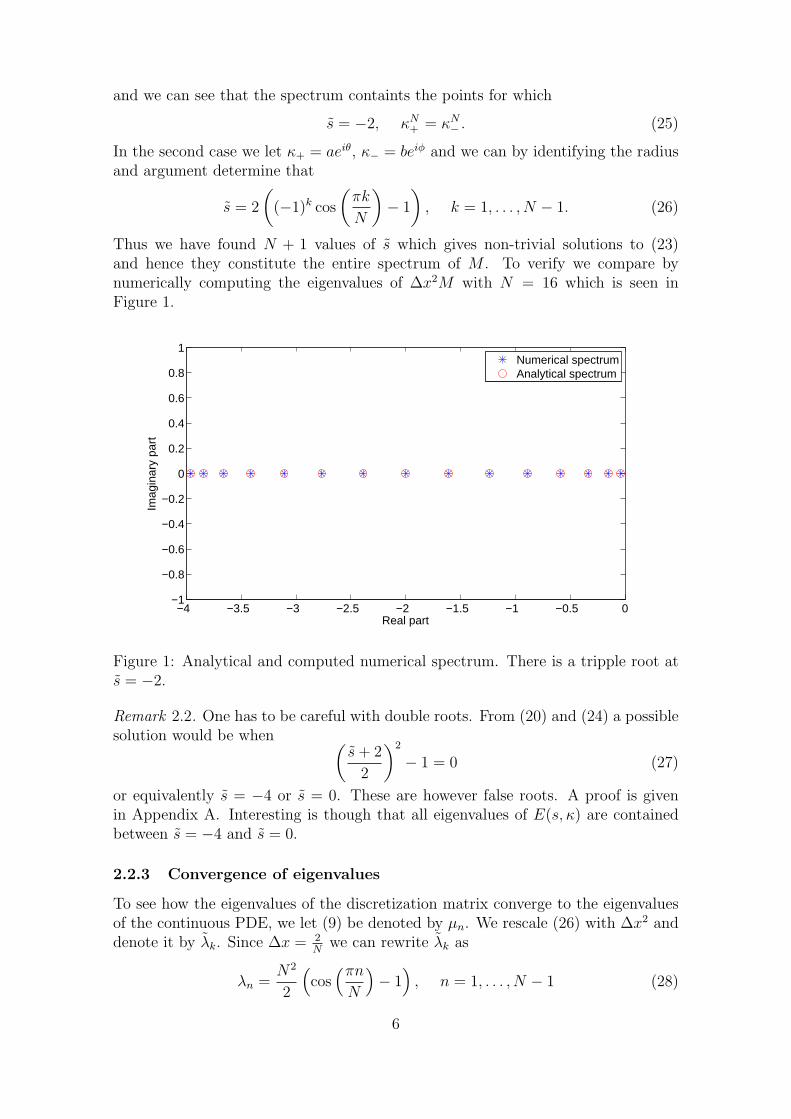
Thus we have found N + 1 values of s which gives non-trivial solutions to (23)and hence they constitute the entire spectrum of M . To verify we compare bynumerically computing the eigenvalues of ∆x2M with N = 16 which is seen inFigure 1.
−4 −3.5 −3 −2.5 −2 −1.5 −1 −0.5 0−1
−0.8
−0.6
−0.4
−0.2
0
0.2
0.4
0.6
0.8
1
Real part
Imag
inar
y pa
rt
Numerical spectrumAnalytical spectrum
Figure 1: Analytical and computed numerical spectrum. There is a tripple root ats = −2.
Remark 2.2. One has to be careful with double roots. From (20) and (24) a possiblesolution would be when (
s+ 2
2
)2
− 1 = 0 (27)
or equivalently s = −4 or s = 0. These are however false roots. A proof is givenin Appendix A. Interesting is though that all eigenvalues of E(s, κ) are containedbetween s = −4 and s = 0.
2.2.3 Convergence of eigenvalues
To see how the eigenvalues of the discretization matrix converge to the eigenvaluesof the continuous PDE, we let (9) be denoted by µn. We rescale (26) with ∆x2 anddenote it by λk. Since ∆x = 2
Nwe can rewrite λk as
λn =N2
2
(cos(πnN
)− 1), n = 1, . . . , N − 1 (28)
6
which generates the same sequence as (26), but it is monotonically decreasing. Thisallows us to compare µn and λn elementwise.
By assuming that n < N we can Taylor expand (28) around zero and simplifyto get
λn = µn +O
(n4
N2
). (29)
We can see that for large N we can expect the first√N eigenvalues to be rather
well approximated while for larger n than that, they will start to diverge. This isthe typical situation. When the resolution is increased, more eigenvalues will beconverged but eigenvalues that are not converging will be created.
3 Multi domain spectral analysis of the heat equa-
tion
In this section we shall use the knowledge obtained in the previous section to de-termine spectral properties when an artificial interface has been introduced in thedomain. Our goal is to determine how the introduction of an interface influencesthe spectrum of both the continuous and discrete equations. Moreover we want todesign the interface treatment in such a way that it is similar to, or maybe evenbetter than, the single domain spectrum if possible.
3.1 Continuous case
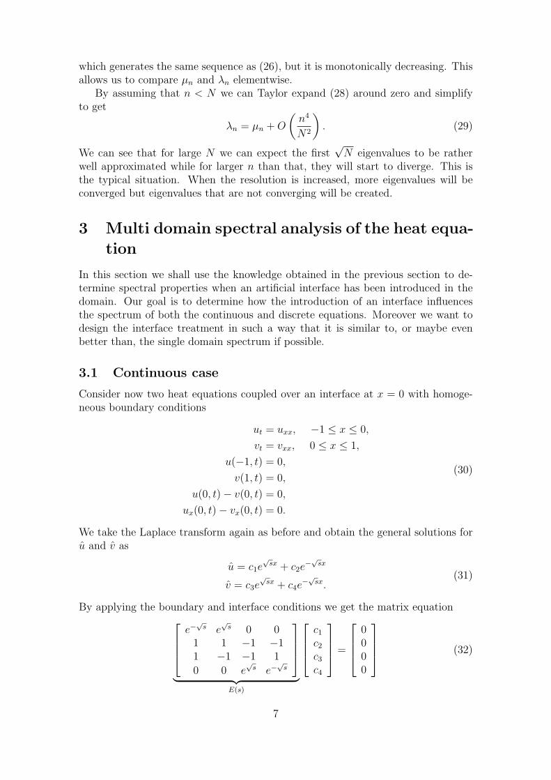
Consider now two heat equations coupled over an interface at x = 0 with homoge-neous boundary conditions
ut = uxx, −1 ≤ x ≤ 0,
vt = vxx, 0 ≤ x ≤ 1,
u(−1, t) = 0,
v(1, t) = 0,
u(0, t)− v(0, t) = 0,
ux(0, t)− vx(0, t) = 0.
(30)
We take the Laplace transform again as before and obtain the general solutions foru and v as
u = c1e√sx + c2e
−√sx
v = c3e√sx + c4e
−√sx.
(31)
By applying the boundary and interface conditions we get the matrix equatione−√s e
√s 0 0
1 1 −1 −11 −1 −1 1
0 0 e√s e−
√s
︸ ︷︷ ︸
E(s)
c1c2c3c4
=
0000
(32)
7

with a non-trivial solution when det(E(s)) = 0. A direct computation of the de-terminant shows that det(E(s)) = 4 sinh(2
√s) and hence the spectrum remains
unchanged by the introduction of an interface. This is of course all in order sincethe interface is purely artificial. However when we discretize (30) we modify thescheme at the interface and we can expect that this modification will influence theeigenvalues of the complete difference operator.
3.2 Discrete case
In order to proceed we assume that there are equally many grid points in eachsubdomain and that the grid spacing is the same. This means that we can applythe same operators in both domains which will simplify the notation and algebra.
With a slight abuse of notation we now let u and v denote the discrete gridfunctions with both having N + 1 components. Thus there are in total 2N + 2 gridpoints in the domain since the interface point occurs twice, and the resolution istwice as high as in the single domain case.
By using the SBP and SAT technique we can discretize (30) as
ut = D2u+ σ1P−1DTE0u
+ σ2P−1DT eN(uN − v0) + σ3P
−1eN((Du)N − (Dv)0)
vt = D2v + τ1P−1DTENv
+ τ2P−1DT e0(v0 − uN) + τ3P
−1e0((Dv)0 − (Du)N)
(33)
The unknown penalty parameters σ1,2,3 and τ1,2,3 has again to be determined forstability.
3.2.1 Stability
To determine the unknown parameters σ1,2,3 and τ1,2,3 we multiply the first equationin (33) with uTP and the second with vTP . We add the transposes of the resultingexpressions to themselves to get
||u||2t = −2u0(Du)0 + 2uN(Du)N − uT (A+ AT )u
+ 2σ1(Du)0u0 + 2σ2(Du)N(uN − v0) + 2σ3uM((Du)N − (Dv)0)
||v||2t = −2v0(Dv)0 + 2vN(Dv)N − vT (A+ AT )v
+ 2τ1(Dv)NvN + 2τ2(Dv)0(v0 − uN) + 2τ3v0((Dv)0 − (Du)N).
(34)
By adding both expressions in (34) we can write the result as
||u||2t + ||v||2t = 2(σ1 − 1)u0(Du)0 + 2(τ1 + 1)vN(Dv)N
+ qTHq − uT (A+ AT )u− vT (A+ AT )v(35)
where q = [uN , (Du)N , v0, (Dv)0]T and
H =
0 1 + σ2 + σ3 0 −(τ2 + τ3)
1 + σ2 + σ3 0 −(τ2 + τ3) 00 −(σ2 + τ3) 0 −1 + τ2 + τ3
−(σ3 + τ2) 0 −1 + τ2 + τ3 0
. (36)
8

In order to bound (35) we have to choose
σ1 = 1, τ1 = −1 (37)
as in the single domain case, and we have to choose the rest of the penalty parameterssuch that H ≤ 0. This is easily accomplished by noting that the diagonal of Hconsists of zeros only, and hence by the Gershgorin theorem we need to put allremaining entires to zero to ensure the semidefiniteness of H. This gives us a one-parameter family of solutions
r ∈ R, σ2 = −(1 + r), σ3 = r, τ2 = −r, τ3 = 1 + r. (38)
Thus all penalty parameters have been determined and the scheme is stable.Worth noting is that the parameter r determines how the equations are coupled.
For r = 0 two of the penalty parameters in (38) disappear and renders the schemeone-sided coupled in the sense that the left domain receives a solution value fromthe right domain and gives the value of its gradient to the right domain. For r = −1the situation is reversed and for other values of r, the scheme is fully coupled. Notethat the scheme is stable for all choices of r. We shall investigate the influence ofthe interface paramater in later sections. More details can also be found in [6].
3.2.2 Eigenspectrum
The scheme (33) with a second order accurate difference operator makes eight gridpoints (two at each boundary and four at the interface) stray from a standard cen-tral finite difference scheme. This is a significant modification and we can expectthat there will be a global impact depending on these modifications. A direct wayof investigating this is by considering the change on the spectrum due to the modi-fications.
We take the Laplace transform of (33) and consider the difference equations atthe modified boundary and interface points. We get after substituting (37) and (38)into (33) that
(s+ 2)u0 = 0
−2u0 + (s+ 2)u1 − u2 = 0
−uN−2 + (s+ 2)uN−1 − (2 + r)uN + (1 + r)v0 = 0
2ruN−1 + (s+ 2)uN − 2(1 + 2r)v0 + 2rv1 = 0
−2(1 + r)uN−1 + 2(1 + 2r)uN + (s+ 2)v0 − 2(1 + r)v1 = 0
−ruN − (1− r)v0 + (s+ 2)v1 − v2 = 0
−vN−2 + (s+ 2)vN−1 − 2vN = 0
(s+ 2)vN = 0.
(39)
From the internal schemes we have similarly as before that
ui = c1κi+ + c2κ
i−
vj = c3κj+ + c4κ
j−
(40)
9
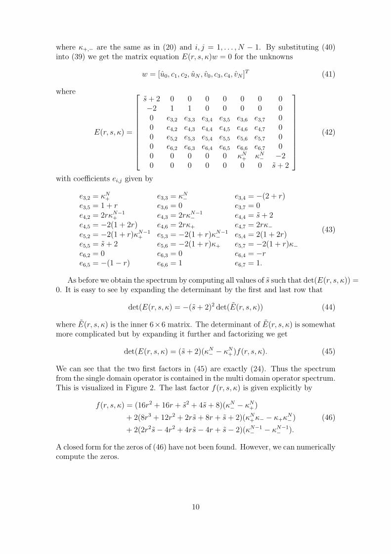
where κ+,− are the same as in (20) and i, j = 1, . . . , N − 1. By substituting (40)into (39) we get the matrix equation E(r, s, κ)w = 0 for the unknowns
w = [u0, c1, c2, uN , v0, c3, c4, vN ]T (41)
where
E(r, s, κ) =
s+ 2 0 0 0 0 0 0 0−2 1 1 0 0 0 0 00 e3,2 e3,3 e3,4 e3,5 e3,6 e3,7 00 e4,2 e4,3 e4,4 e4,5 e4,6 e4,7 00 e5,2 e5,3 e5,4 e5,5 e5,6 e5,7 00 e6,2 e6,3 e6,4 e6,5 e6,6 e6,7 00 0 0 0 0 κN+ κN− −20 0 0 0 0 0 0 s+ 2
(42)
with coefficients ei,j given by
e3,2 = κN+ e3,3 = κN− e3,4 = −(2 + r)e3,5 = 1 + r e3,6 = 0 e3,7 = 0e4,2 = 2rκN−1
+ e4,3 = 2rκN−1− e4,4 = s+ 2
e4,5 = −2(1 + 2r) e4,6 = 2rκ+ e4,7 = 2rκ−e5,2 = −2(1 + r)κN−1
+ e5,3 = −2(1 + r)κN−1− e5,4 = 2(1 + 2r)
e5,5 = s+ 2 e5,6 = −2(1 + r)κ+ e5,7 = −2(1 + r)κ−e6,2 = 0 e6,3 = 0 e6,4 = −re6,5 = −(1− r) e6,6 = 1 e6,7 = 1.
(43)
As before we obtain the spectrum by computing all values of s such that det(E(r, s, κ)) =0. It is easy to see by expanding the determinant by the first and last row that
det(E(r, s, κ) = −(s+ 2)2 det(E(r, s, κ)) (44)
where E(r, s, κ) is the inner 6×6 matrix. The determinant of E(r, s, κ) is somewhatmore complicated but by expanding it further and factorizing we get
det(E(r, s, κ) = (s+ 2)(κN− − κN+ )f(r, s, κ). (45)
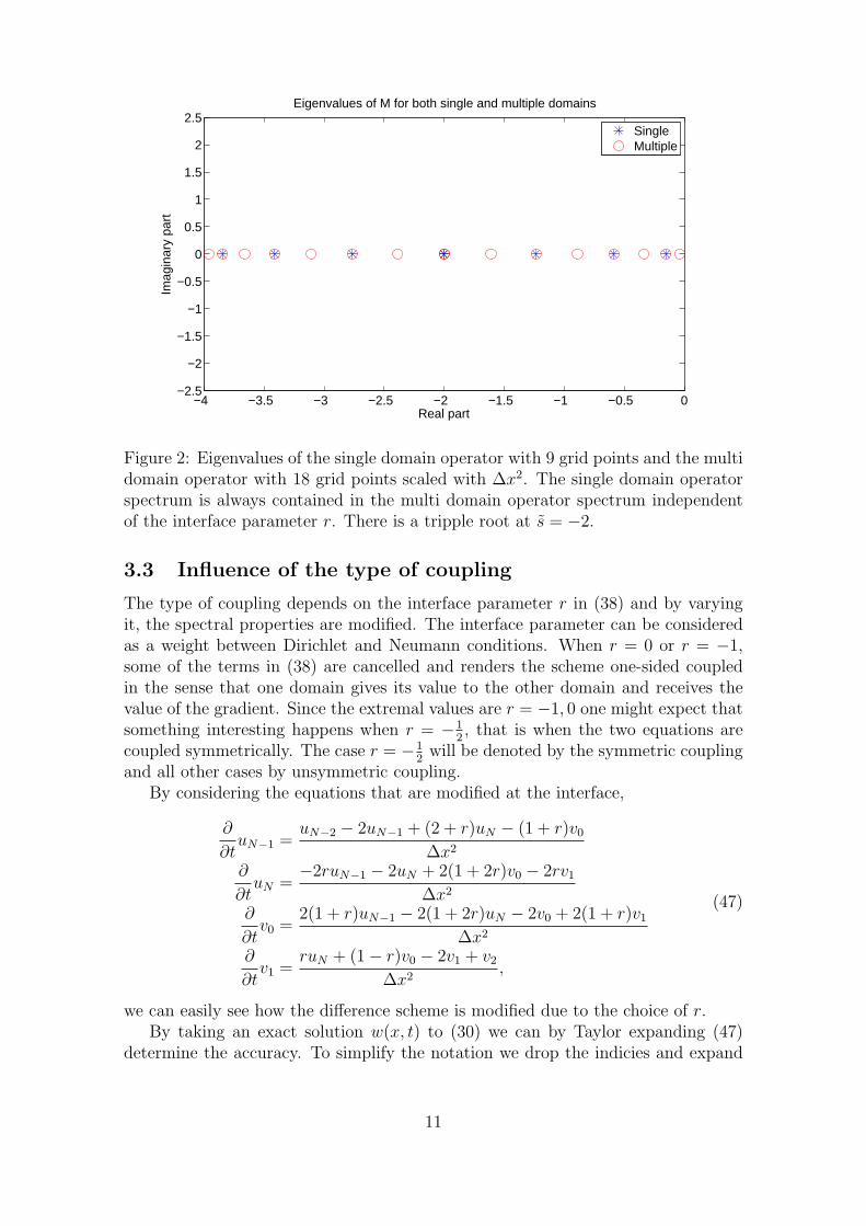
We can see that the two first factors in (45) are exactly (24). Thus the spectrumfrom the single domain operator is contained in the multi domain operator spectrum.This is visualized in Figure 2. The last factor f(r, s, κ) is given explicitly by
f(r, s, κ) = (16r2 + 16r + s2 + 4s+ 8)(κN− − κN+ )
+ 2(8r3 + 12r2 + 2rs+ 8r + s+ 2)(κN+κ− − κ+κN− )
+ 2(2r2s− 4r2 + 4rs− 4r + s− 2)(κN−1− − κN−1
− ).
(46)
A closed form for the zeros of (46) have not been found. However, we can numericallycompute the zeros.
10
−4 −3.5 −3 −2.5 −2 −1.5 −1 −0.5 0−2.5
−2
−1.5
−1
−0.5
0
0.5
1
1.5
2
2.5
Real part
Imag
inar
y pa
rt
Eigenvalues of M for both single and multiple domains
SingleMultiple
Figure 2: Eigenvalues of the single domain operator with 9 grid points and the multidomain operator with 18 grid points scaled with ∆x2. The single domain operatorspectrum is always contained in the multi domain operator spectrum independentof the interface parameter r. There is a tripple root at s = −2.
3.3 Influence of the type of coupling
The type of coupling depends on the interface parameter r in (38) and by varyingit, the spectral properties are modified. The interface parameter can be consideredas a weight between Dirichlet and Neumann conditions. When r = 0 or r = −1,some of the terms in (38) are cancelled and renders the scheme one-sided coupledin the sense that one domain gives its value to the other domain and receives thevalue of the gradient. Since the extremal values are r = −1, 0 one might expect thatsomething interesting happens when r = −1
2, that is when the two equations are
coupled symmetrically. The case r = −12
will be denoted by the symmetric couplingand all other cases by unsymmetric coupling.
By considering the equations that are modified at the interface,
∂
∂tuN−1 =
uN−2 − 2uN−1 + (2 + r)uN − (1 + r)v0
∆x2
∂
∂tuN =
−2ruN−1 − 2uN + 2(1 + 2r)v0 − 2rv1
∆x2
∂
∂tv0 =
2(1 + r)uN−1 − 2(1 + 2r)uN − 2v0 + 2(1 + r)v1
∆x2
∂
∂tv1 =
ruN + (1− r)v0 − 2v1 + v2
∆x2,
(47)
we can easily see how the difference scheme is modified due to the choice of r.By taking an exact solution w(x, t) to (30) we can by Taylor expanding (47)
determine the accuracy. To simplify the notation we drop the indicies and expand
11
all equations around xj = x∗. We get
∂
∂tw(x∗, t) = wxx(x∗, t) +O(∆x2)
∂
∂tw(x∗, t) = −2rwxx(x∗, t) +O(∆x2)
∂
∂tw(x∗, t) = 2(1 + r)wxx(x∗, t) +O(∆x2)
∂
∂tw(x∗, t) = wxx(x∗, t) +O(∆x2)
(48)
for the corresponding equations in (47). We can now easily see that we obtain thesecond order accurate second derivative only for r = −1
2. Even though some of the
above equations correspond to inconsistent approximations of the second derivative,the global accuracy of the operator remain unchanged [7, 13, 12].
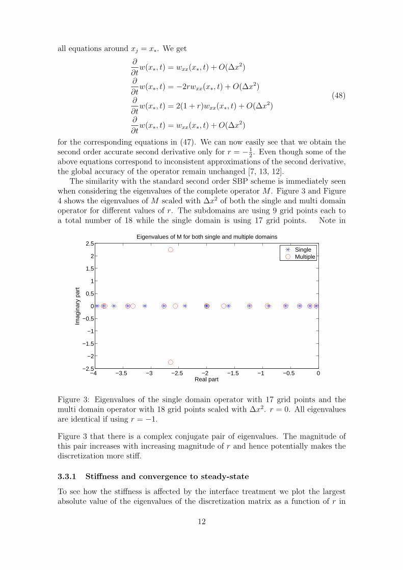
The similarity with the standard second order SBP scheme is immediately seenwhen considering the eigenvalues of the complete operator M . Figure 3 and Figure4 shows the eigenvalues of M scaled with ∆x2 of both the single and multi domainoperator for different values of r. The subdomains are using 9 grid points each toa total number of 18 while the single domain is using 17 grid points. Note in
−4 −3.5 −3 −2.5 −2 −1.5 −1 −0.5 0−2.5
−2
−1.5
−1
−0.5
0
0.5
1
1.5
2
2.5
Real part
Imag
inar
y pa
rt
Eigenvalues of M for both single and multiple domains
SingleMultiple
Figure 3: Eigenvalues of the single domain operator with 17 grid points and themulti domain operator with 18 grid points scaled with ∆x2. r = 0. All eigenvaluesare identical if using r = −1.
Figure 3 that there is a complex conjugate pair of eigenvalues. The magnitude ofthis pair increases with increasing magnitude of r and hence potentially makes thediscretization more stiff.
3.3.1 Stiffness and convergence to steady-state
To see how the stiffness is affected by the interface treatment we plot the largestabsolute value of the eigenvalues of the discretization matrix as a function of r in
12
−4 −3.5 −3 −2.5 −2 −1.5 −1 −0.5 0−2.5
−2
−1.5
−1
−0.5
0
0.5
1
1.5
2
2.5
Real part
Imag
inar
y pa
rt
Eigenvalues of M for both single and multiple domains
SingleMultiple
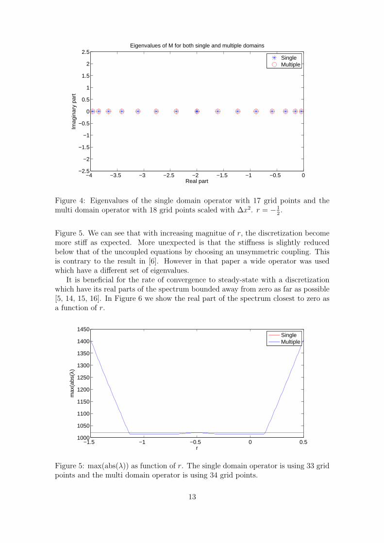
Figure 4: Eigenvalues of the single domain operator with 17 grid points and themulti domain operator with 18 grid points scaled with ∆x2. r = −1
2.
Figure 5. We can see that with increasing magnitue of r, the discretization becomemore stiff as expected. More unexpected is that the stiffness is slightly reducedbelow that of the uncoupled equations by choosing an unsymmetric coupling. Thisis contrary to the result in [6]. However in that paper a wide operator was usedwhich have a different set of eigenvalues.
It is beneficial for the rate of convergence to steady-state with a discretizationwhich have its real parts of the spectrum bounded away from zero as far as possible[5, 14, 15, 16]. In Figure 6 we show the real part of the spectrum closest to zero asa function of r.
−1.5 −1 −0.5 0 0.51000
1050
1100
1150
1200
1250
1300
1350
1400
1450
r
max
(abs
(λ)
SingleMultiple
Figure 5: max(abs(λ)) as function of r. The single domain operator is using 33 gridpoints and the multi domain operator is using 34 grid points.
13

−1.5 −1 −0.5 0 0.5−2.4661
−2.466
−2.4659
−2.4658
−2.4657
−2.4656
−2.4655
−2.4654
−2.4653
r
max
(rea
l(λ)
SingleMultiple
Figure 6: max(R(λ)) as a function of r. The single domain operator is using 33 gridpoints and the multi domain operator is using 34 grid points.
We have used 33 grid points for the single domain in both Figure 5 and Figure6 and hence the coupled domains have 34 grid points in total. The computationof the rightmost lying eigenvalue in Figure 6 is resolved and the variation with r issmall. For a coarse mesh the convergence to steady-state can be slightly improvedby having an unsymmetric coupling. This is again contrary to the result in [6].
3.3.2 Error analysis
We will use the method of manufactured solutions to study the error as a functionof the interface parameter r. Any function v ∈ C2 is a solution to
ut = uxx + F (x, t), −1 ≤ x ≤ 1,
u(x, 0) = v(x, 0)
u(−1, t) = v(−1, t)
u(1, t) = v(1, t)
(49)
where the forcing function F (x, t) has been chosen appropriately. In this particularcase we choose
v(x, t) =sin(2πx− t) + sin(t)
4(50)
which satisfies (49) with homogeneous boundary conditions and
F (x, t) =cos(t)− cos(2πx− t) + π2 sin(2πx− t)
4. (51)
The spatial discretization and stability conditions are the same as before and weuse the classical 4th-order Runge-Kutta time integration scheme to solve a systemof the form
∂ψ
∂t= Mψ + F. (52)
14
All spatial discretization, including boundary and interface conditions, is includedin M and F is the above forcing function in discrete vector form. Thus we have aanalytical solution which we can use to study the errors. In [17] it is stated that theerrors can be reduced depending on the interface coupling for a hyperbolic problemand we will investigate if a similar effect exist for a parabolic problem.
Using the manufactured solution (49) it was verified that the coupled schemeconverges with second order of accuracy independent of the interface parameter r.
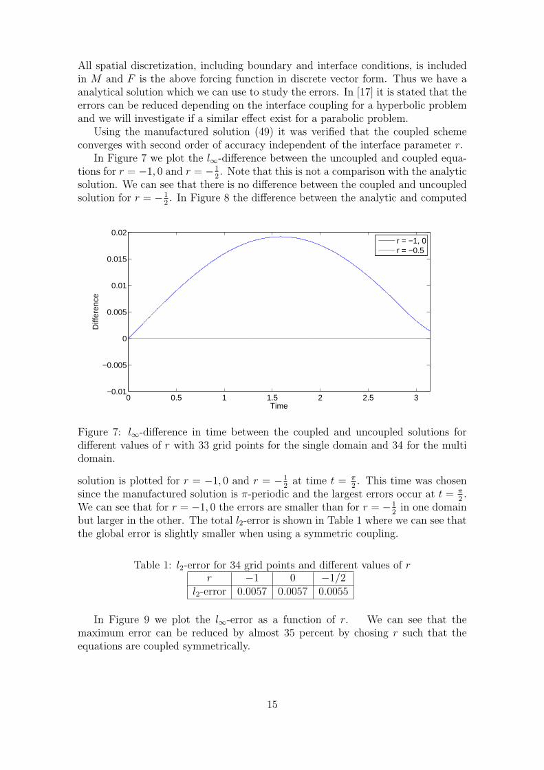
In Figure 7 we plot the l∞-difference between the uncoupled and coupled equa-tions for r = −1, 0 and r = −1
2. Note that this is not a comparison with the analytic
solution. We can see that there is no difference between the coupled and uncoupledsolution for r = −1
2. In Figure 8 the difference between the analytic and computed
0 0.5 1 1.5 2 2.5 3−0.01
−0.005
0
0.005
0.01
0.015
0.02
Time
Diff
eren
ce
r = −1, 0r = −0.5
Figure 7: l∞-difference in time between the coupled and uncoupled solutions fordifferent values of r with 33 grid points for the single domain and 34 for the multidomain.
solution is plotted for r = −1, 0 and r = −12
at time t = π2. This time was chosen
since the manufactured solution is π-periodic and the largest errors occur at t = π2.
We can see that for r = −1, 0 the errors are smaller than for r = −12
in one domainbut larger in the other. The total l2-error is shown in Table 1 where we can see thatthe global error is slightly smaller when using a symmetric coupling.
Table 1: l2-error for 34 grid points and different values of rr −1 0 −1/2
l2-error 0.0057 0.0057 0.0055
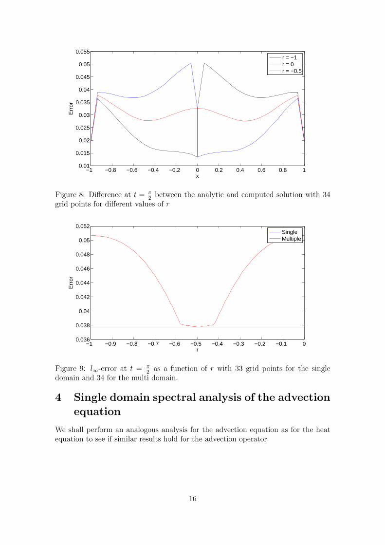
In Figure 9 we plot the l∞-error as a function of r. We can see that themaximum error can be reduced by almost 35 percent by chosing r such that theequations are coupled symmetrically.
15
−1 −0.8 −0.6 −0.4 −0.2 0 0.2 0.4 0.6 0.8 10.01
0.015
0.02
0.025
0.03
0.035
0.04
0.045
0.05
0.055
x
Err
or
r = −1r = 0r = −0.5
Figure 8: Difference at t = π2
between the analytic and computed solution with 34grid points for different values of r
−1 −0.9 −0.8 −0.7 −0.6 −0.5 −0.4 −0.3 −0.2 −0.1 00.036
0.038
0.04
0.042
0.044
0.046
0.048
0.05
0.052
r
Err
or
SingleMultiple
Figure 9: l∞-error at t = π2
as a function of r with 33 grid points for the singledomain and 34 for the multi domain.
4 Single domain spectral analysis of the advection
equation
We shall perform an analogous analysis for the advection equation as for the heatequation to see if similar results hold for the advection operator.
16

4.1 Continuous case
Consider the advection equation in one domain,
ut + ux = 0, −1 ≤ x ≤ 1,
u(−1, t) = g(t),
u(x, 0) = f(x).
(53)
Equation (53) is significantly different from (1) due to the directionality of the spatialoperator. In this case there is one signal travelling from left to right and hence onlyone boundary condition is needed at x = −1. To obtain the spectrum we take theLaplace transform of (53) and proceed as before. We get
su+ ux = 0 (54)
which has the characteristic equation
κ+ s = 0 (55)
and thus the general solution of (54) is
u = ce−sx. (56)
If we apply the boundary condition with g = 0 we get c = 0 and thus u = 0. Hencethere is no continuous spectrum of (53) since there are no values of s such thatces = 0 for c 6= 0.
4.2 Discrete case
We discretize (53) using the SBP and SAT technique on a uniform mesh of N + 1grid points
ut + P−1Qv = σP−1(v0 − g)e0 (57)
where P and e0 are as before and
Q =1
2
−1 1 0 0 · · · 0−1 0 1 0 · · · 0...
. . . . . . . . . . . ....
0 · · · 0 −1 0 10 · · · 0 0 −1 1
, P−1Q =1
2∆x
−2 2 0 0 · · · 0−1 0 1 0 · · · 0...
. . . . . . . . . . . ....
0 · · · 0 1 0 −10 · · · 0 0 −2 2
.(58)
Note that Q+QT = diag(−1, 0, · · · , 0, 1) which is used to select the boundary termsin the energy estimate. By applying the energy method to (57) with g = 0 we get
||v||2t = (1 + 2σ)v20 − v2
N (59)
which is bounded for σ ≤ −12
and hence the scheme is stable.To determine the spectrum we Laplace transform (57) (with g = 0) and rewrite
as(sI + P−1Q− σP−1E0)v = 0. (60)
17

From the internal scheme we have
svi +1
2∆x(vi+1 − vi−1) = 0 (61)
or equivalentlyvi+1 + 2svi − vi−1 = 0 (62)
with s = s∆x. The characteristic equation is κ2 + 2sκ− 1 = 0 which has solutions
κ+,− = −s±√s2 + 1. (63)
Thus the general solution of (62) is
vi = c1κi+ + c2κ
i−. (64)
The first and last equation in (60) are modified and we can use them to write amatrix equation for the unknowns c1,2. The equations are
(s− 1− 2σ)v0 + v1 = 0
−vN−1 + (s+ 1)vN = 0(65)
and by inserting the general solution (64) into (65) we get the matrix equationE(s, κ)c = 0 where
E(s, κ) =
[s− 1− sσ + κ+ s− 1− sσ + κ−
(s+ 1)κN+ − κN−1+ (s+ 1)κN− − κN−1
−
]. (66)
The spectrum consists as before of the singular points of E(s, κ). A direct compu-tation of the determinant of E(s, κ) gives that
det(E(s, κ)) = κN− (√s2 + 1− 1− 2σ)(1 +
√s2 + 1)
+ κN+ (√s2 + 1 + 1 + 2σ)(1−
√s2 + 1).
(67)
A closed form expression for the zeros of (67) have not been found. We can howevercompute the eigenvalues numerically. We will return to (67) when we consider thespectrum of the coupled problem.
5 Multi domain spectral analysis of the advection
equation
We introduce again an artificial interface at x = 0 for the advection equation to studyhow the spectral properties of the continuous and discrete operators are modified.
5.1 Continuous case
Consider now
ut + ux = 0, −1 ≤ x ≤ 0,
vt + vx = 0, 0 ≤ x ≤ 1,
u(−1, t) = g(t),
v(0, t) = u(0, t).
(68)
18
The spectrum is again obtained by Laplace transforming (68) and applying theboundary and interface conditions. The general solutions to the Laplace transformedequations are u = c1e
−sx and v = c2e−sx. The boundary and interface conditions
imply that c1 = 0 and c2 = c1, and hence there is no spectrum as expected.
5.2 Discrete case
One form of the SBP and SAT discretization of (68) is
ut + P−1Qu = σP−1(u0 − g)e0
vt + P−1Qv = τP−1(v0 − uN)e0(69)
where u, v now denote the discrete grid functions. Both domains have equidistantgrid spacing and equal number of grid points to allow for the same difference oper-ators in both domains.
5.2.1 Conservation and stability
When constructing an interface for equations with advection it is important thatthe scheme is not only stable, but also conservative [1, 18, 10]. Let Φ(x) be asmooth testfunction and let φ = [Φ(x0), . . . ,Φ(xN)]T . We multiply both equationsin (69) with φTP respectively. By using the SBP property of Q and adding the twoequations we can shift the differentiation onto φ and get
φTPut+φTPvt−φ0u0 +φNvN−(Qφ)Tu−(Qφ)Tv−σφ0(u0−g) = φi(τ+1)(v0−uN)
(70)where we have used φ0 = Φ(−1), φN = Φ(1) and φi = Φ(0) to denote the boundaryand interface points. To ensure that the interface is conservative we cannot haveany remaining interface terms and hence we need to put τ = −1 to cancel the termsin the right hand side of (70). With this choice we thus have a conservative interfacetreatment.
To determine the stability condition we proceed with the energy method as beforeby multiplying both equations in (69) with uTP and vTP respectively. By assumingthat g = 0 we get
||u||2t + ||v||2t = (1 + 2σ)u20 + (1 + τ)v2
0 − v2N − (uN + τv0)
2 (71)
and we can see that the scheme is stable if we chose σ ≤ −12
and τ ≤ −1. Thus theinterface treatment is both stable and conservative with τ = −1.
5.2.2 Eigenspectrum
We Laplace transform (69) and get the general solution from the internal schemesas before,
ui = c1κi+ + c2κ
i−
vi = c3κi+ + c4κ
i−,
(72)
19
where κ+,− = −s ±√s2 + 1. The scheme at the boundaries and interfaces are
different from the internal scheme and their corresponding equations are
(s− 1− 2σ)u0 + u1 = 0
(s+ 1)uN − uN−1 = 0
2τ uN + (s− 1− 2τ)v0 + v1 = 0
(s+ 1)vN − vN−1 = 0.
(73)
By inserting the general solutions into (73) we get again the matrix equation E(s, κ)c =0 for the unknowns c = [c1, . . . , c4]
T where
E(s, κ) =
s− 1− 2σ + κ+ s− 1− 2σ + κ− 0 0
(s+ 1)κN+ − κN−1+ (s+ 1)κN− − κN−1
− 0 02τκN+ 2τκN− s− 1− 2τ + κ+ s− 1− 2τ + κ−
0 0 (s+ 1)κN+ − κN−1+ (s+ 1)κN− − κN−1
−
.(74)
The spectrum is obtained for the singular values of E(s, κ). By expanding thedeterminant of E(s, κ) and factorizing we get
det(E(s, κ)) = f(σ, s)g(τ, s) (75)
where
f(σ, s) = κN− (√s2 + 1− 1− 2σ)(1 +
√s2 + 1)
+ κN+ (√s2 + 1 + 1 + 2σ)(1−
√s2 + 1)
(76)
is exactly (67). The second factor is
g(τ, s) = (s2 − 1− 2τ s− 2τ + sκ+ + κ+)κN−
− (s2 − 1− 2τ s− 2τ + sκ− + κ−)κN+
− (s− 1− 2τ + κ+)κN−1− + (s− 1− 2τ + κ−)κN−1.
(77)
We can see that the single domain operator spectrum is again contained in themulti domain operator spectrum, which is visualized in Figure 10 and Figure 11for σ = −1
2and σ = −1 respectively. In the second case, which is fully upwinded,
we can see that the spectrum is identical for the single and multi domain operatorssince all eigenvalues of the multi domain operator are double eigenvalues.
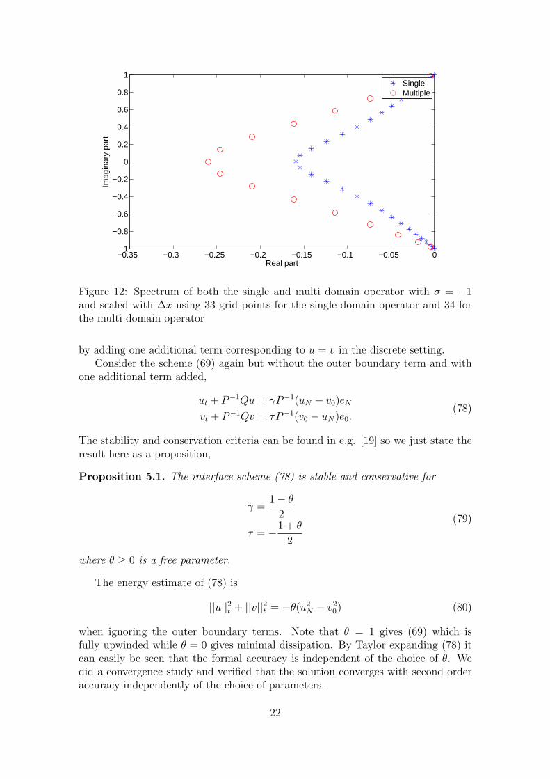
Figure 12 shows the spectrum of both the single and multi domain operators for33 and 34 grid points respectively and σ = −1. We can see that the spectrum ofthe operators does not agree as they did in the coupled diffusion case. Note againthat all eigenvalues of the multi domain operator are double eigenvalues.
5.3 Extending the interface treatment
In the previous section we discussed one of many different schemes for the advectionequation coupled over an interface. The scheme was based on the boundary andinterface conditions for the continuous PDE. The interface condition v = u is of
20

−0.35 −0.3 −0.25 −0.2 −0.15 −0.1 −0.05 0−1
−0.8
−0.6
−0.4
−0.2
0
0.2
0.4
0.6
0.8
1
Real part
Imag
inar
y pa
rt
SingleMultiple
Figure 10: Spectrum of both the single and multi domain operator with σ = −12
and scaled with ∆x, using 17 grid points for the single domain operator and 34 forthe multi domain operator. The single domain operator spectrum is contained inthe multi domain operator spectrum.
−0.35 −0.3 −0.25 −0.2 −0.15 −0.1 −0.05 0−1
−0.8
−0.6
−0.4
−0.2
0
0.2
0.4
0.6
0.8
1
Real part
Imag
inar
y pa
rt
SingleMultiple
Figure 11: Spectrum of both the single and multi domain operator with σ = −1and scaled with ∆x, using 17 grid points for the single domain operator and 34 forthe multi domain operator. The multi domain operator spectrum is identical to thesingle domain operator spectrum since all eigenvalues of the multi domain operatorare double eigenvalues.
course identical to u = v in the continuous sense, but this is not true in the discretesetting with weak interface conditions. We can hence modify the interface treatment
21
−0.35 −0.3 −0.25 −0.2 −0.15 −0.1 −0.05 0−1
−0.8
−0.6
−0.4
−0.2
0
0.2
0.4
0.6
0.8
1
Real part
Imag
inar
y pa
rt
SingleMultiple
Figure 12: Spectrum of both the single and multi domain operator with σ = −1and scaled with ∆x using 33 grid points for the single domain operator and 34 forthe multi domain operator
by adding one additional term corresponding to u = v in the discrete setting.Consider the scheme (69) again but without the outer boundary term and with
one additional term added,
ut + P−1Qu = γP−1(uN − v0)eN
vt + P−1Qv = τP−1(v0 − uN)e0.(78)
The stability and conservation criteria can be found in e.g. [19] so we just state theresult here as a proposition,
Proposition 5.1. The interface scheme (78) is stable and conservative for
γ =1− θ
2
τ = −1 + θ
2
(79)
where θ ≥ 0 is a free parameter.
The energy estimate of (78) is
||u||2t + ||v||2t = −θ(u2N − v2
0) (80)
when ignoring the outer boundary terms. Note that θ = 1 gives (69) which isfully upwinded while θ = 0 gives minimal dissipation. By Taylor expanding (78) itcan easily be seen that the formal accuracy is independent of the choice of θ. Wedid a convergence study and verified that the solution converges with second orderaccuracy independently of the choice of parameters.
22
5.3.1 Stiffness, convergence and errors
In the case of advection there are two free parameters compared to the diffusioncase where there is only one. One parameter for the outer boundary −∞ ≤ σ ≤ −1
2
and one parameter for the interface 0 ≤ θ ≤ ∞. Since we are interested only inthe interface treatment we let σ = −1 be fixed and consider the stiffness, rate ofconvergence and error as a function of θ.
In [17] the quasi-one-dimensional Euler equations were used with an interfacetreatment corresponding to θ = 1 to study the errors. Their convergence studyshowed that the errors were small and does not increase with the number of sub-domains. We continue with a more detailed investigation by posing the errors asfunctions of the interface treatment.
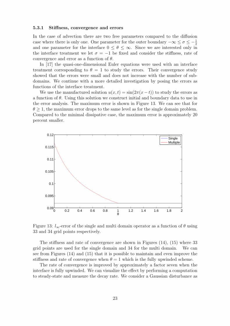
We use the manufactured solution u(x, t) = sin(2π(x− t)) to study the errors asa function of θ. Using this solution we construct initial and boundary data to use inthe error analysis. The maximum error is shown in Figure 13. We can see that forθ ≥ 1, the maximum error drops to the same level as for the single domain problem.Compared to the minimal dissipative case, the maximum error is approximately 20percent smaller.
0 0.2 0.4 0.6 0.8 1 1.2 1.4 1.6 1.8 20.09
0.095
0.1
0.105
0.11
0.115
0.12
θ
SingleMultiple
Figure 13: l∞-error of the single and multi domain operator as a function of θ using33 and 34 grid points respectively.
The stiffness and rate of convergence are shown in Figures (14), (15) where 33grid points are used for the single domain and 34 for the multi domain. We cansee from Figures (14) and (15) that it is possible to maintain and even improve thestiffness and rate of convergence when θ = 1 which is the fully upwinded scheme.
The rate of convergence is improved by approximately a factor seven when theinterface is fully upwinded. We can visualize the effect by performing a computationto steady-state and measure the decay rate. We consider a Gaussian disturbance as
23

0 0.2 0.4 0.6 0.8 1 1.2 1.4 1.6 1.8 215
20
25
30
35
40
45
50
55
60
θ
Stif
fnes
s
SingleMultiple
Figure 14: max(abs(λ)) as function of θ. The single domain operator is using 33grid points and the multi domain operator is using 34 grid points.
0 0.2 0.4 0.6 0.8 1 1.2 1.4 1.6 1.8 2−0.08
−0.07
−0.06
−0.05
−0.04
−0.03
−0.02
−0.01
0
θ
Con
verg
ence
rat
e
SingleMultiple
Figure 15: max(R(λ)) as a function of θ. The single domain operator is using 33grid points and the multi domain operator is using 34 grid points.
initial data with initial position x0 = −12. The initial data is given explicitly by
f(x) = e−100(x−x0)2 . (81)
The disturbance is transported out of the boundary and the exact steady-state so-lution is identically zero. To investigate what effect multiple interfaces have wecompute in time until the l2-norm of the solution is less than 10−16, which is con-sidered to be the steady-state solution. The result is seen in Table 2 for the single
24
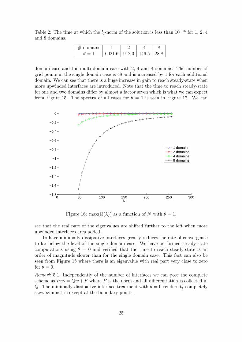
Table 2: The time at which the l2-norm of the solution is less than 10−16 for 1, 2, 4and 8 domains.
# domains 1 2 4 8θ = 1 6021.6 912.0 146.5 28.8
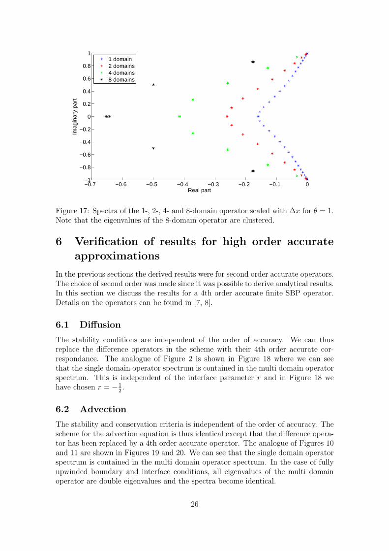
domain case and the multi domain case with 2, 4 and 8 domains. The number ofgrid points in the single domain case is 48 and is increased by 1 for each additionaldomain. We can see that there is a huge increase in gain to reach steady-state whenmore upwinded interfaces are introduced. Note that the time to reach steady-statefor one and two domains differ by almost a factor seven which is what we can expectfrom Figure 15. The spectra of all cases for θ = 1 is seen in Figure 17. We can
0 50 100 150 200 250 300−1.8
−1.6
−1.4
−1.2
−1
−0.8
−0.6
−0.4
−0.2
0
N
1 domain2 domains4 domains8 domains
Figure 16: max(R(λ)) as a function of N with θ = 1.
see that the real part of the eigenvalues are shifted further to the left when moreupwinded interfaces area added.
To have minimally dissipative interfaces greatly reduces the rate of convergenceto far below the level of the single domain case. We have performed steady-statecomputations using θ = 0 and verified that the time to reach steady-state is anorder of magnitude slower than for the single domain case. This fact can also beseen from Figure 15 where there is an eigenvalue with real part very close to zerofor θ = 0.
Remark 5.1. Independently of the number of interfaces we can pose the completescheme as Pwt = Qw+F where P is the norm and all differentiation is collected inQ. The minimally dissipative interface treatment with θ = 0 renders Q completelyskew-symmetric except at the boundary points.
25
−0.7 −0.6 −0.5 −0.4 −0.3 −0.2 −0.1 0−1
−0.8
−0.6
−0.4
−0.2
0
0.2
0.4
0.6
0.8
1
Real part
Imag
inar
y pa
rt
1 domain2 domains4 domains8 domains
Figure 17: Spectra of the 1-, 2-, 4- and 8-domain operator scaled with ∆x for θ = 1.Note that the eigenvalues of the 8-domain operator are clustered.
6 Verification of results for high order accurate
approximations
In the previous sections the derived results were for second order accurate operators.The choice of second order was made since it was possible to derive analytical results.In this section we discuss the results for a 4th order accurate finite SBP operator.Details on the operators can be found in [7, 8].
6.1 Diffusion
The stability conditions are independent of the order of accuracy. We can thusreplace the difference operators in the scheme with their 4th order accurate cor-respondance. The analogue of Figure 2 is shown in Figure 18 where we can seethat the single domain operator spectrum is contained in the multi domain operatorspectrum. This is independent of the interface parameter r and in Figure 18 wehave chosen r = −1
2.
6.2 Advection
The stability and conservation criteria is independent of the order of accuracy. Thescheme for the advection equation is thus identical except that the difference opera-tor has been replaced by a 4th order accurate operator. The analogue of Figures 10and 11 are shown in Figures 19 and 20. We can see that the single domain operatorspectrum is contained in the multi domain operator spectrum. In the case of fullyupwinded boundary and interface conditions, all eigenvalues of the multi domainoperator are double eigenvalues and the spectra become identical.
26

−15 −10 −5 0−1
−0.8
−0.6
−0.4
−0.2
0
0.2
0.4
0.6
0.8
1
Real part
Imag
inar
y pa
rt
Eigenvalues of M for both single and multiple domains
SingleMultiple
Figure 18: Eigenvalues of the 4th order accurate single domain diffusion operatorwith 9 grid points and the multi domain operator with 18 grid points scaled with∆x2. The single domain operator spectrum is always contained in the multi domainoperator spectrum independent of the interface parameter r. Here r = −1
2.
−0.4 −0.35 −0.3 −0.25 −0.2 −0.15 −0.1 −0.05 0−2
−1.5
−1
−0.5
0
0.5
1
1.5
2
Real part
Imag
inar
y pa
rt
SingleMultiple
Figure 19: Spectrum of both the single and multi domain advection operator withσ = −1
2and scaled with ∆x, using 17 grid points for the 4th order accurate single
domain operator and 34 for the multi domain operator. The single domain operatorspectrum is contained in the multi domain operator spectrum.
7 Summary and conclusions
We have used a second order accurate finite difference method on Summation-By-Parts form to discretize the heat- and advection equation on single and multiple
27

−0.4 −0.35 −0.3 −0.25 −0.2 −0.15 −0.1 −0.05 0−2
−1.5
−1
−0.5
0
0.5
1
1.5
2
Real part
Imag
inar
y pa
rt
SingleMultiple
Figure 20: Spectrum of both the single and multi domain advection operator withσ = −1 and scaled with ∆x, using 17 grid points for the 4th order accurate singledomain operator and 34 for the multi domain operator. The multi domain operatorspectrum is identical to the single domain operator spectrum since all eigenvaluesof the multi domain operator are double eigenvalues.
domains. The results are differing between the diffusion and advection case and wediscuss them separately.
In both cases we derived an interface treatment which is depending on an inter-face parameter which can be used to alter the interface treatment. We studied whichimpact the interface treatment has on the spectrum, stiffness, rate of convergenceand errors. In both cases we showed how the spectrum of the single domain operatoris included in the multi domain operator spectrum and that the result carry over tohigher order accurate approximations.
7.1 Diffusion
In the single domain case, a closed form expression for all eigenvalues of the dis-cretization matrix, including the boundary conditions, was found. We showed howthe eigenvalues of the discretization matrix converged to the eigenvalues of the con-tinuous equation. For the multiple domain case we showed how the spectrum ofthe single domain operator is contained in the multi domain operator spectrumindependent of the interface treatment.
The stiffness and rate of convergence were not significantly effected by the choiceof interface treatment. We used a manufactured solution to study the errors. Whenthe symmetric coupling was used, the maximum error of the multi domain casereduced to the level of the single domain case. Compared to the unsymmetric cou-pling, the maximum errors were reduced by almost 35 percent when the symmetriccoupling was used.
28

7.2 Advection
For the advection equation we showed that the spectrum of the single domain opera-tor is contained in the multi domain operator spectrum independent of the interfacetreatment similarly to the diffusion case.
The stiffness showed only minor differences depending on the interface treatment.The rate of convergence to steady-state was improved by approximately a factorseven when adding one upwinded interface. By adding more upwinded interfaceswe could dramatically decrease the computational time to reach the steady-statesolution. When the interface treatment was chosen minimally dissipative the schemebecomes completely skew-symmetric and the rate of convergence to steady-state wasseverely decreased due to the presence of an eigenvalue with almost zero real part.
We used an exact solution to study the errors as a function of the interfacetreatment. We showed that it is possible to bring down the maximum errors to thelevel of the single domain case by using the upwinded coupling. The maximum errorwas about 20 percent smaller when using a fully upwinded coupling compared tothe minimal dissipative coupling.
References
[1] Jan Nordstrom, Jing Gong, Edwin van der Weide, and Magnus Svard. A stableand conservative high order multi-block method for the compressible Navier-Stokes equations. Journal of Computational Physics, 228(24):9020–9035, 2009.
[2] Jan Nordstrom and Magnus Svard. Well-Posed Boundary Conditions for theNavier–Stokes Equations. SIAM Journal on Numerical Analysis, 43(3):1231–1255, 2005.
[3] Magnus Svard, Mark H. Carpenter, and Jan Nordstrom. A stable high-orderfinite difference scheme for the compressible Navier-Stokes equations, far-fieldboundary conditions. Journal of Computational Physics, 225(1):1020–1038,2007.
[4] Magnus Svard and Jan Nordstrom. A stable high-order finite difference schemefor the compressible Navier-Stokes equations: No-slip wall boundary conditions.Journal of Computational Physics, 227(10):4805 – 4824, 2008.
[5] Magnus Svard, Ken Mattsson, and Jan Nordstrom. Steady-State Computa-tions Using Summation-by-Parts Operators. Journal of Scientific Computing,24(1):79–95, 2005.
[6] Jens Lindstrom and Jan Nordstrom. A stable and high-order accurate conjugateheat transfer problem. Journal of Computational Physics, 229(14):5440–5456,2010.
[7] Ken Mattsson and Jan Nordstrom. Summation by parts operators for finitedifference approximations of second derivatives. Journal of ComputationalPhysics, 199(2):503–540, 2004.
29
[8] Bo Strand. Summation by Parts for Finite Difference Approximations for d/dx.Journal of Computational Physics, 110(1):47 – 67, 1994.
[9] Bertil Gustafsson, Heinz-Otto Kreiss, and Joseph Oliger. Time DependentProblems and Difference Methods. Wiley Interscience, 1995.
[10] Mark H. Carpenter, Jan Nordstrom, and David Gottlieb. Revisiting and extend-ing interface penalties for multi-domain summation-by-parts operators. Journalof Scientific Computing, 45(1-3):118–150, 2010.
[11] Sofia Eriksson and Jan Nordstrom. Analysis of the order of accuracy for node-centered finite volume schemes. Applied Numerical Mathematics, 59(10):2659– 2676, 2009.
[12] Magnus Svard and Jan Nordstrom. On the order of accuracy for differenceapproximations of initial-boundary value problems. Journal of ComputationalPhysics, 218(1):333–352, 2006.
[13] Ken Mattsson. Boundary Procedures for Summation-by-Parts Operators. Jour-nal of Scientific Computing, 18(1):133–153, 2003.
[14] Bjorn Engquist and Bertil Gustafsson. Steady state computations for wavepropagation problems. Mathematics of Computation, 49(179):39–64, 1987.
[15] Jan Nordstrom. The influence of open boundary conditions on the convergenceto steady state for the Navier-Stokes equations. Journal of ComputationalPhysics, 85(1):210 – 244, 1989.
[16] Peter Eliasson, Sofia Eriksson, and Jan Nordstrom. The influence of weak andstrong solid wall boundary conditions on the convergence to steady-state ofthe Navier-Stokes equations. In Proc. 19th AIAA CFD Conference, number2009-3551 in Conference Proceeding Series. AIAA, 2009.
[17] X. Huan, J.E. Hicken, and D.W. Zingg. Interface and Boundary Schemes forHigh-Order Methods. In the 39th AIAA Fluid Dynamics Conference, AIAAPaper No. 2009-3658, San Antonio, USA, 22–25 June 2009.
[18] Mark H. Carpenter, Jan Nordstrom, and David Gottlieb. A Stable and Con-servative Interface Treatment of Arbitrary Spatial Accuracy. Journal of Com-putational Physics, 148(2):341 – 365, 1999.
[19] Sofia Eriksson, Qaisar Abbas, and Jan Nordstrom. A stable and conserva-tive method for locally adapting the design order of finite difference schemes.Journal of Computational Physics, In Press, Accepted Manuscript:–, 2010.
A Double roots
When determining the solutions to the recurrence relation from the Laplace trans-formed scheme in the interior, one has to be careful with double roots of the char-acteristic equation. Due to the ansatz, false roots might be introduced and it isnecessary to confirm whether or not these roots belong to the spectrum.
30

The characteristic equation (19) has double roots for s = −4 and s = 0. Thesolutions are
κ = −1, κ = 1 (82)
respectively. The general solution to the recurrence relation is then
vi = (c1 + c2i)κi. (83)
We assume that the general solution (83) is valid for i = 1, . . . N − 1 and insert intothe modified boundary equations to get the matrix equation E(s, κ)c = 0 for theunknowns c = [v0, c1, c2, vN ]T where
E(s, κ) =
s+ 2 0 0 0−2 ((s+ 2)− κ)κ ((s+ 2)− 2κ)κ 00 ((s+ 2)κ− 1)κN−2 ((s+ 2)(N − 1)κ− (N − 2))κN−2 −20 0 0 s+ 2
.(84)
By inserting s = −4 and κ = −1 into (84) we get det(E(s, κ)) = 4N(−1)N 6= 0. Byinserting s = 0 and κ = 1 into (84) we get det(E(s, κ)) = 4N 6= 0. Hence neithers = −4 nor s = 0 is a part of the spectrum.
31