spectral and electrical graph theory · 2011-05-17 · graph theory daniel a. spielman ... d i...
TRANSCRIPT
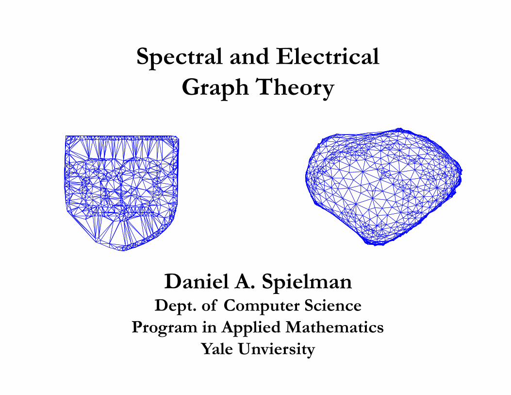
Spectral and Electrical Graph Theory
Daniel A. Spielman Dept. of Computer Science
Program in Applied Mathematics Yale Unviersity
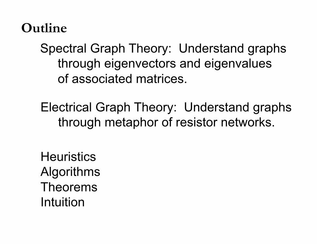
Outline Spectral Graph Theory: Understand graphs through eigenvectors and eigenvalues of associated matrices.
Electrical Graph Theory: Understand graphs through metaphor of resistor networks.
Heuristics Algorithms Theorems Intuition

Spectral Graph Theory
Graph G = (V,E)
Matrix A
rows and cols indexed by
Eigenvalues
Eigenvectors
Av = λv
v : V → IR
V

Spectral Graph Theory
Graph G = (V,E)
Matrix A
rows and cols indexed by
Eigenvalues
Eigenvectors
Av = λv
v : V → IR
1! 2! 3! 4!
1! 2! 3! 4!−1 −0.618 0.618 1
A(i, j) = 1 if (i, j) ∈ EV
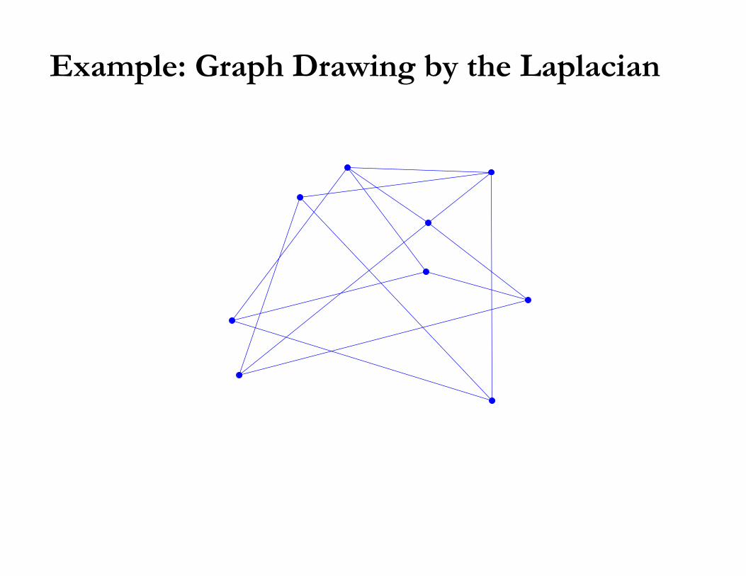
Example: Graph Drawing by the Laplacian

Example: Graph Drawing by the Laplacian
3 1 2
4
5 6 7
8 9
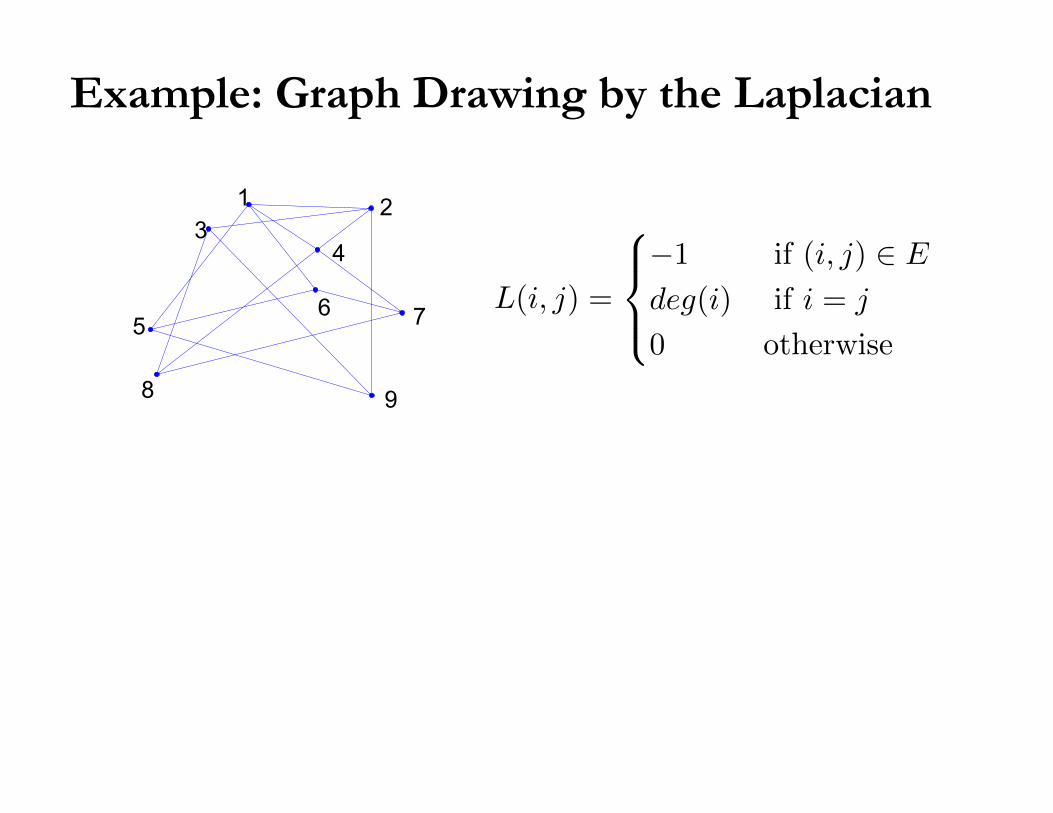
Example: Graph Drawing by the Laplacian
31 2
4
56 7
8 9
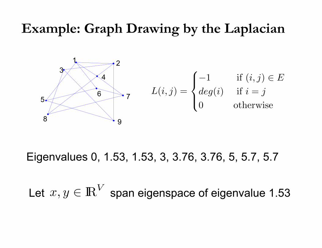
L(i, j) =
−1 if (i, j) ∈ E
deg(i) if i = j
0 otherwise
Example: Graph Drawing by the Laplacian
31 2
4
56 7
8 9
L(i, j) =
−1 if (i, j) ∈ E
deg(i) if i = j
0 otherwise
Eigenvalues 0, 1.53, 1.53, 3, 3.76, 3.76, 5, 5.7, 5.7
Let span eigenspace of eigenvalue 1.53 x, y ∈ IRV
Example: Graph Drawing by the Laplacian
1 2
4
5
6
9
3
8
7
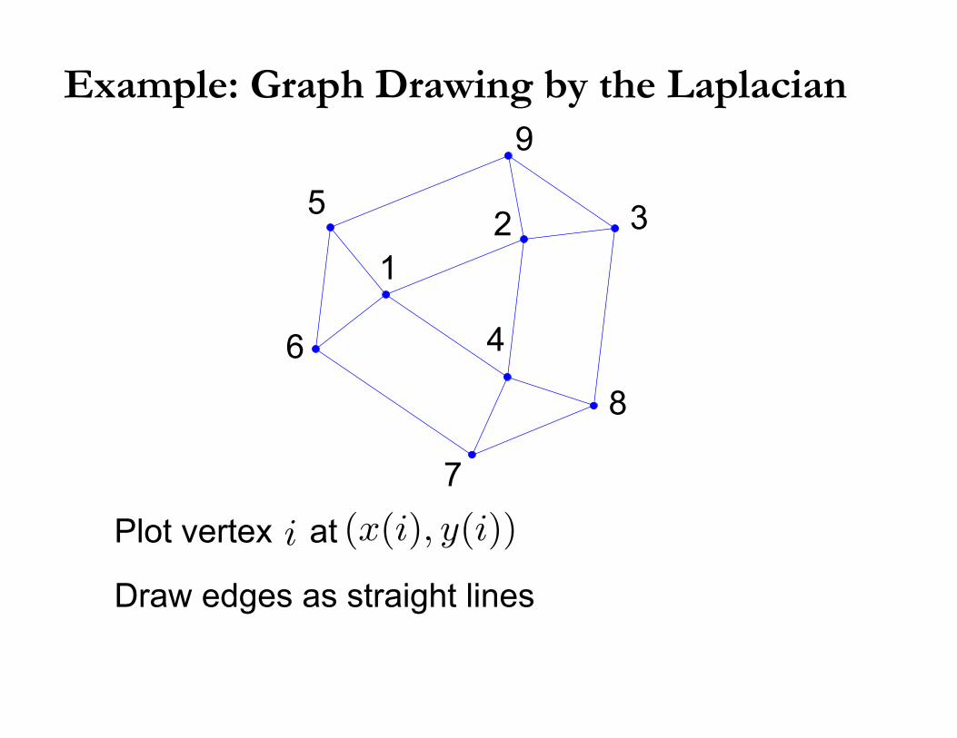
Plot vertex at i (x(i), y(i))
Draw edges as straight lines
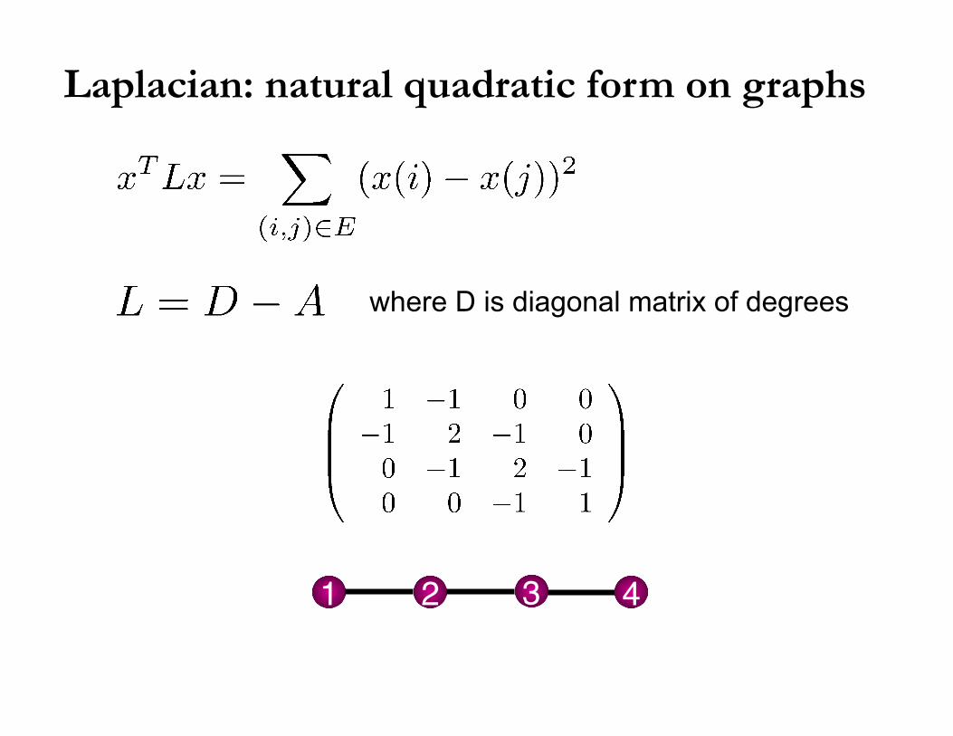
Laplacian: natural quadratic form on graphs
where D is diagonal matrix of degrees
1! 2! 3! 4!

Laplacian: fast facts
zero is an eigenvalue
Connected if and only if
Fiedler (‘73) called “algebraic connectivity of a graph” The further from 0, the more connected.
λ2 > 0
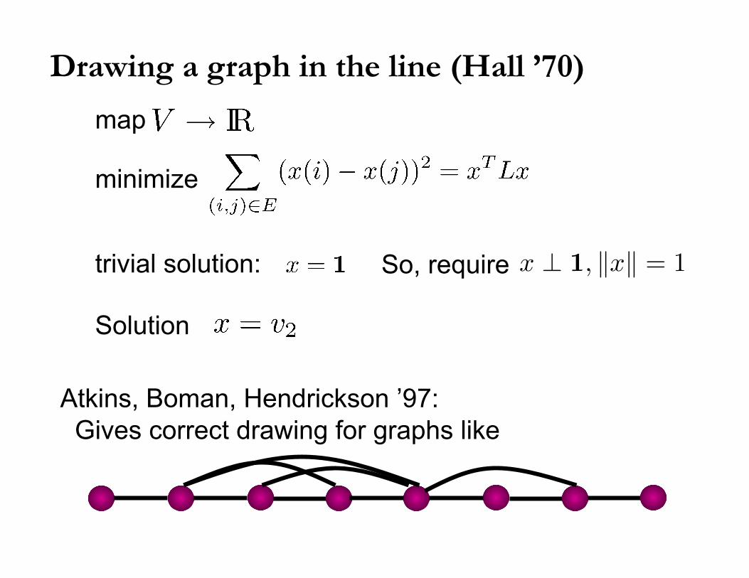
Drawing a graph in the line (Hall ’70)
map
minimize
trivial solution: So, require
Solution
Atkins, Boman, Hendrickson ’97: Gives correct drawing for graphs like
x ⊥ 1, �x� = 1

Courant-Fischer definition of eigvals/vecs

Courant-Fischer definition of eigvals/vecs
(here )
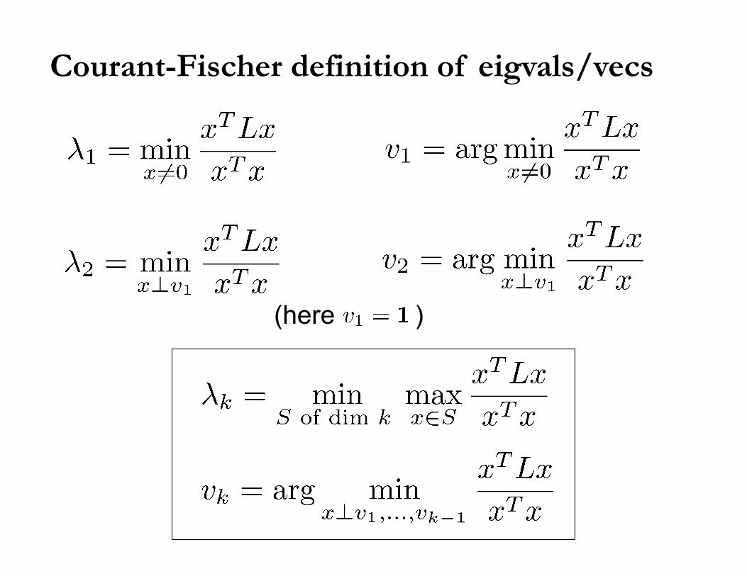
Courant-Fischer definition of eigvals/vecs
(here )

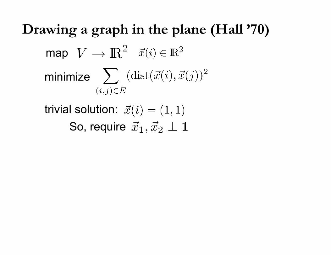
Drawing a graph in the plane (Hall ’70)
minimize
map
Drawing a graph in the plane (Hall ’70)
minimize
map
trivial solution: So, require �x1, �x2 ⊥ 1
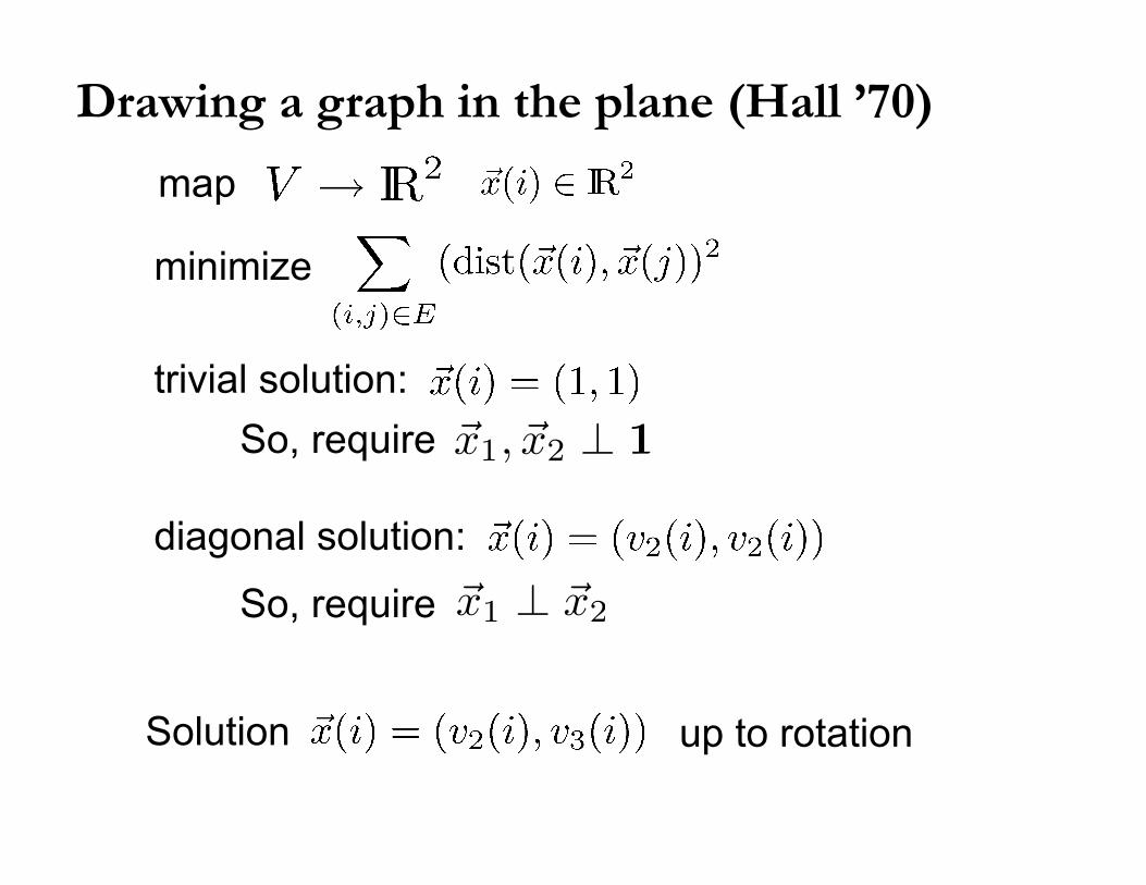
Drawing a graph in the plane (Hall ’70)
minimize
map
trivial solution:
So, require
Solution up to rotation
So, require
diagonal solution: �x1 ⊥ �x2
�x1, �x2 ⊥ 1
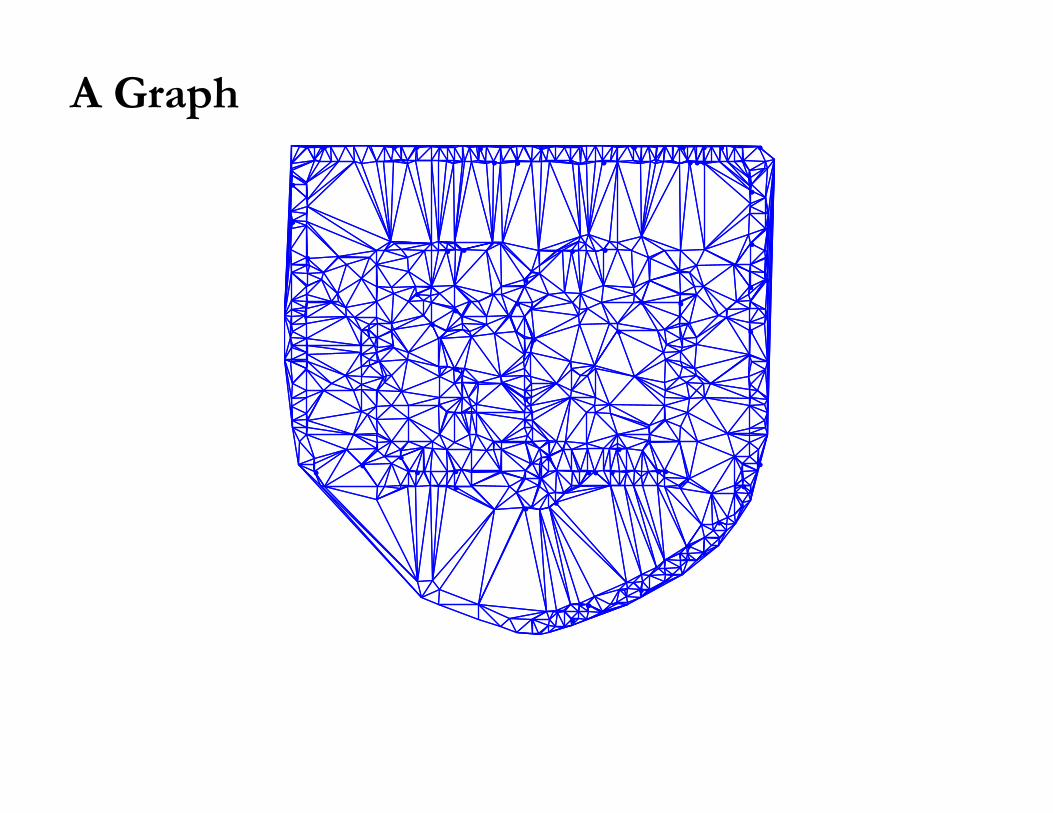
A Graph
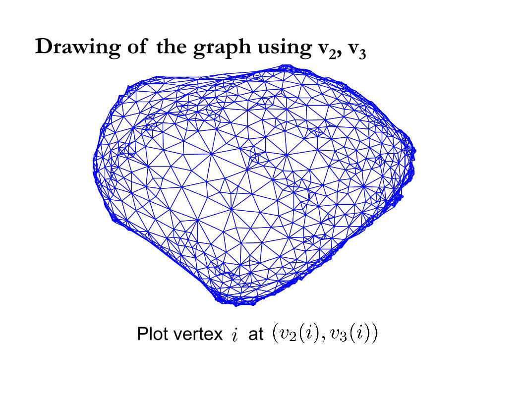
Drawing of the graph using v2, v3
Plot vertex at i
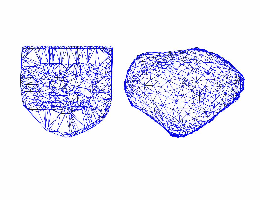

The Airfoil Graph, original coordinates
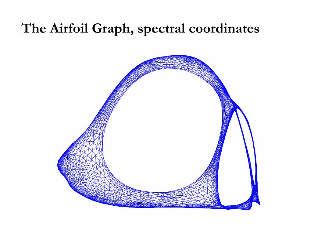
The Airfoil Graph, spectral coordinates
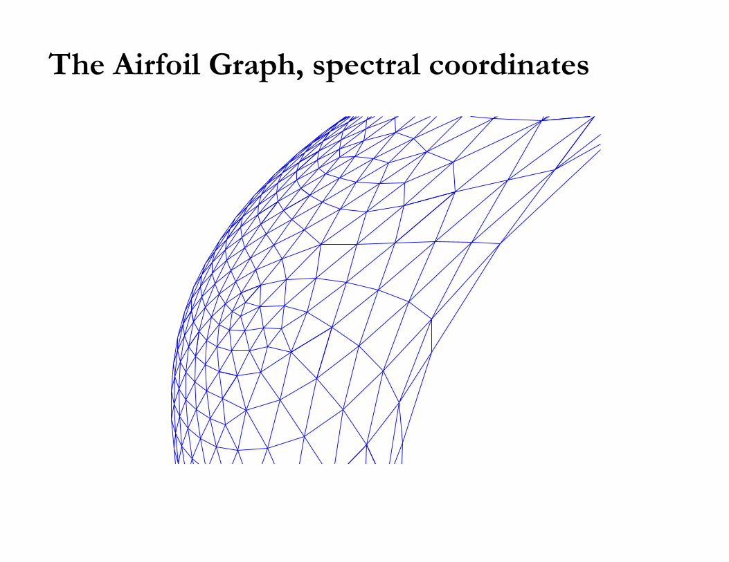
The Airfoil Graph, spectral coordinates
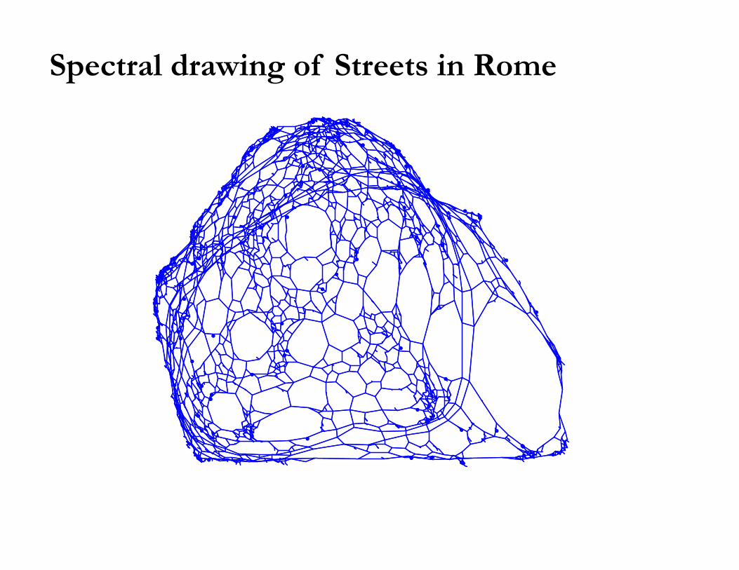
Spectral drawing of Streets in Rome
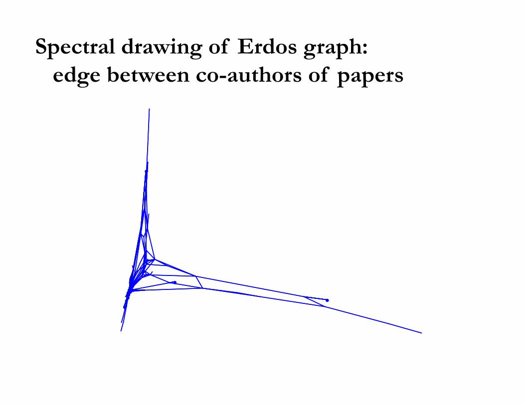
Spectral drawing of Erdos graph: edge between co-authors of papers
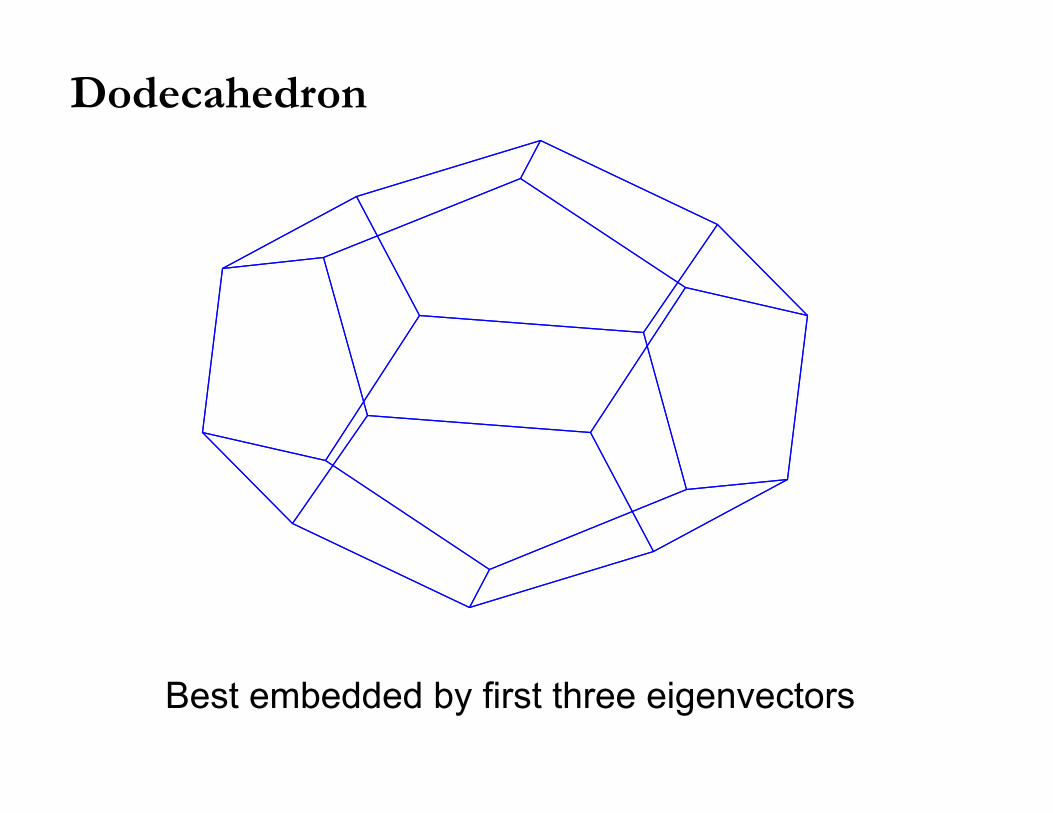
Dodecahedron
Best embedded by first three eigenvectors
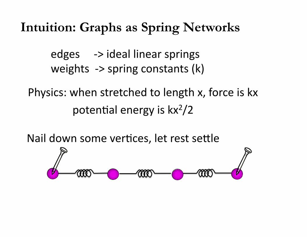
edges -‐> ideal linear springs weights -‐> spring constants (k)
Nail down some ver9ces, let rest se;le
Physics: when stretched to length x, force is kx poten9al energy is kx2/2
Intuition: Graphs as Spring Networks
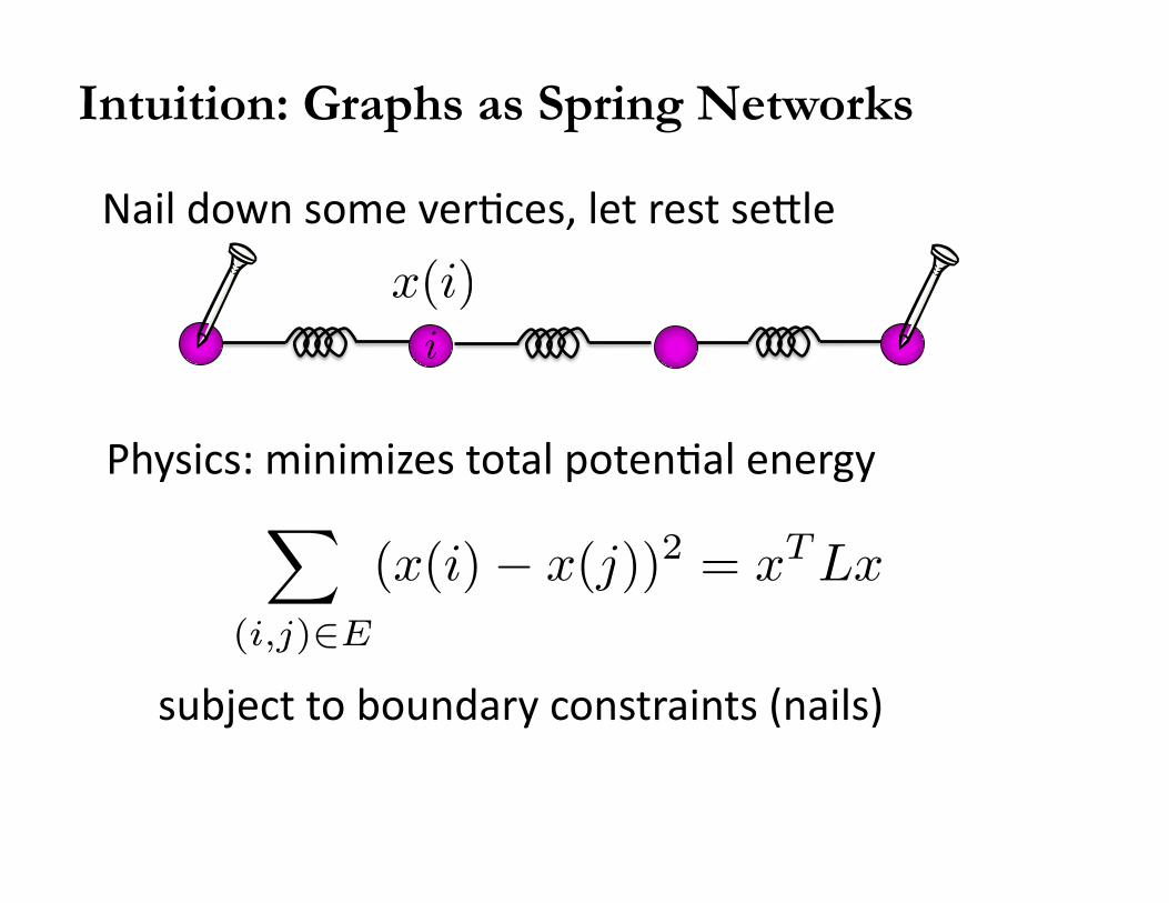
Nail down some ver9ces, let rest se;le
Physics: minimizes total poten9al energy
subject to boundary constraints (nails)
i
Intuition: Graphs as Spring Networks
�
(i,j)∈E
(x(i)− x(j))2 = xTLx
x(i)
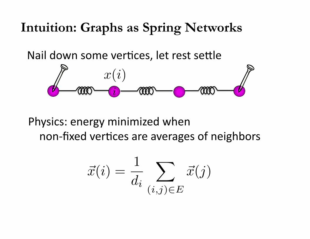
Nail down some ver9ces, let rest se;le
Physics: energy minimized when non-‐fixed ver9ces are averages of neighbors
i
Intuition: Graphs as Spring Networks
x(i)
�x(i) =1
di
�
(i,j)∈E
�x(j)
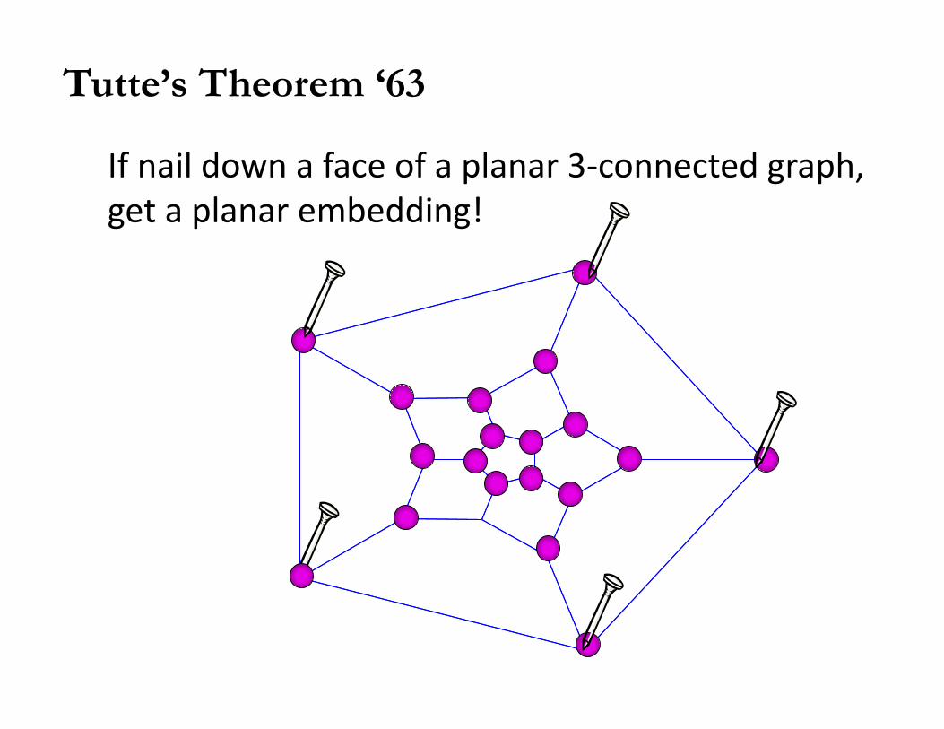
If nail down a face of a planar 3-‐connected graph, get a planar embedding!
Tutte’s Theorem ‘63
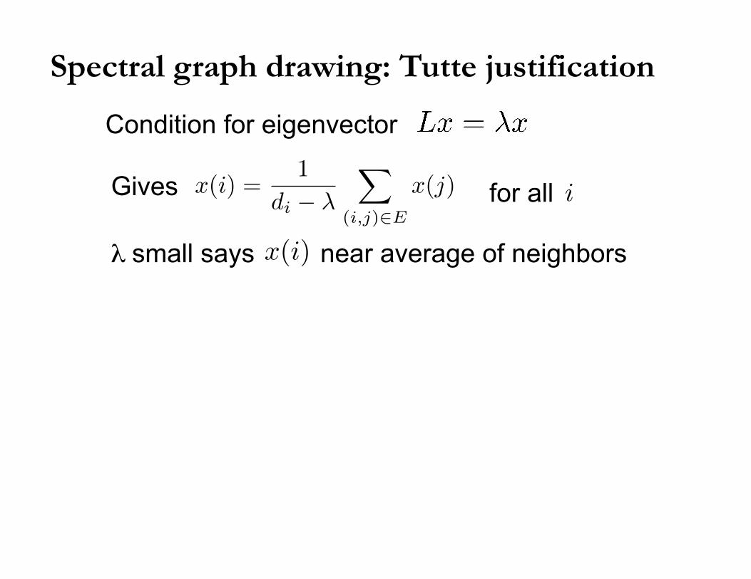
Condition for eigenvector
Spectral graph drawing: Tutte justification
Gives for all
λ small says near average of neighbors
x(i) =1
di − λ
�
(i,j)∈E
x(j)
x(i)
i

Condition for eigenvector
Spectral graph drawing: Tutte justification
Gives for all i
λ small says near average of neighbors
x(i) =1
di − λ
�
(i,j)∈E
x(j)
x(i)
For planar graphs:
λ2 ≤ 8d/n [S-Teng ‘96]
λ3 ≤ O(d/n) [Kelner-Lee-Price-Teng ‘09]

Small eigenvalues are not enough
Plot vertex at i (v3(i), v4(i))
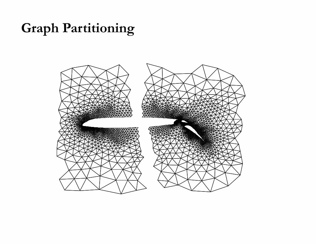
Graph Partitioning
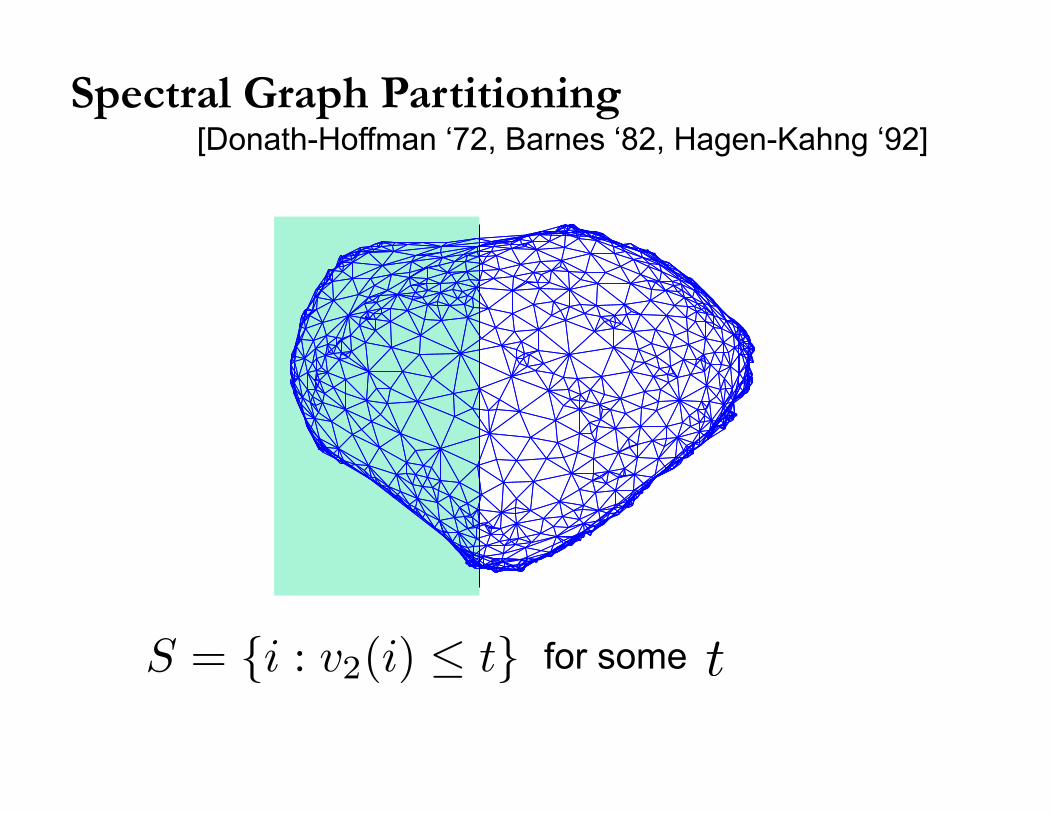
Spectral Graph Partitioning
for some S = {i : v2(i) ≤ t}
[Donath-Hoffman ‘72, Barnes ‘82, Hagen-Kahng ‘92]
t
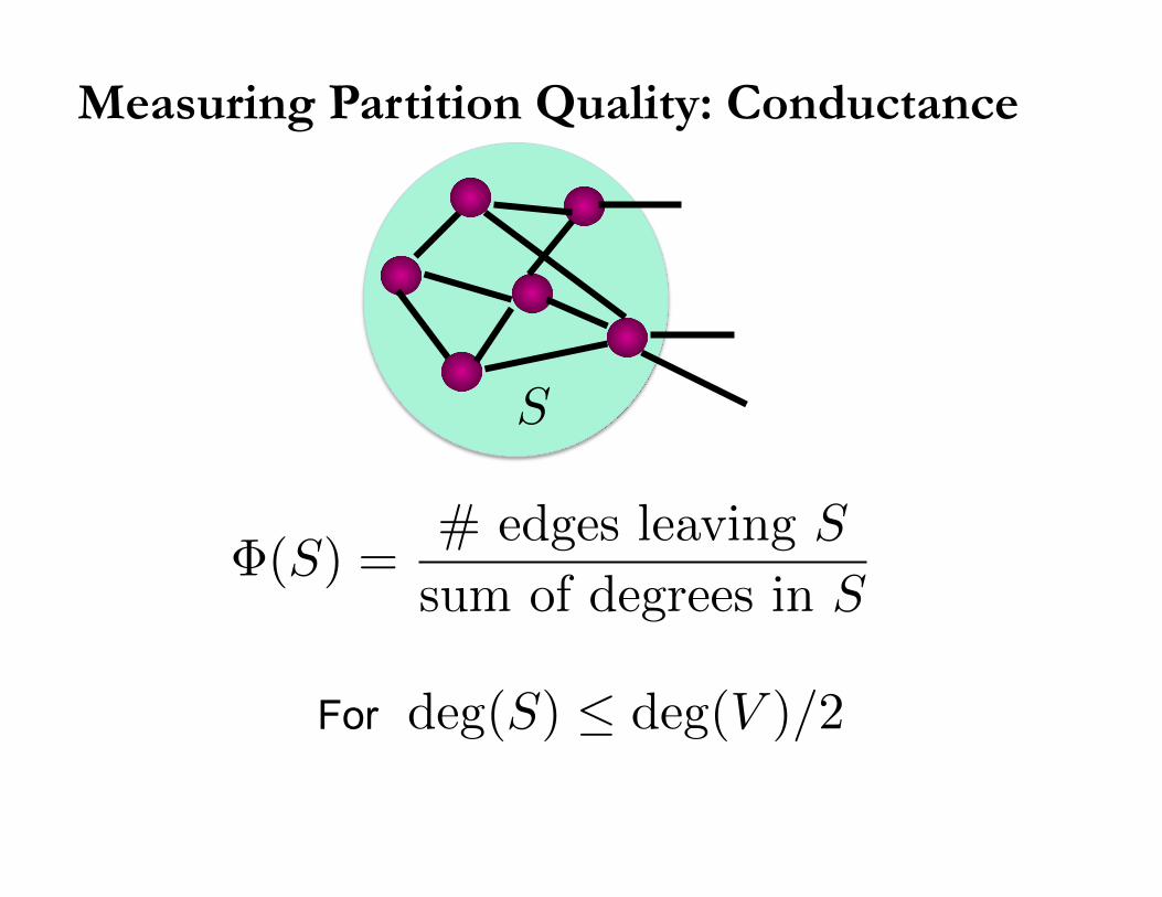
Measuring Partition Quality: Conductance
Φ(S) =# edges leaving S
sum of degrees in S
S
For deg(S) ≤ deg(V )/2

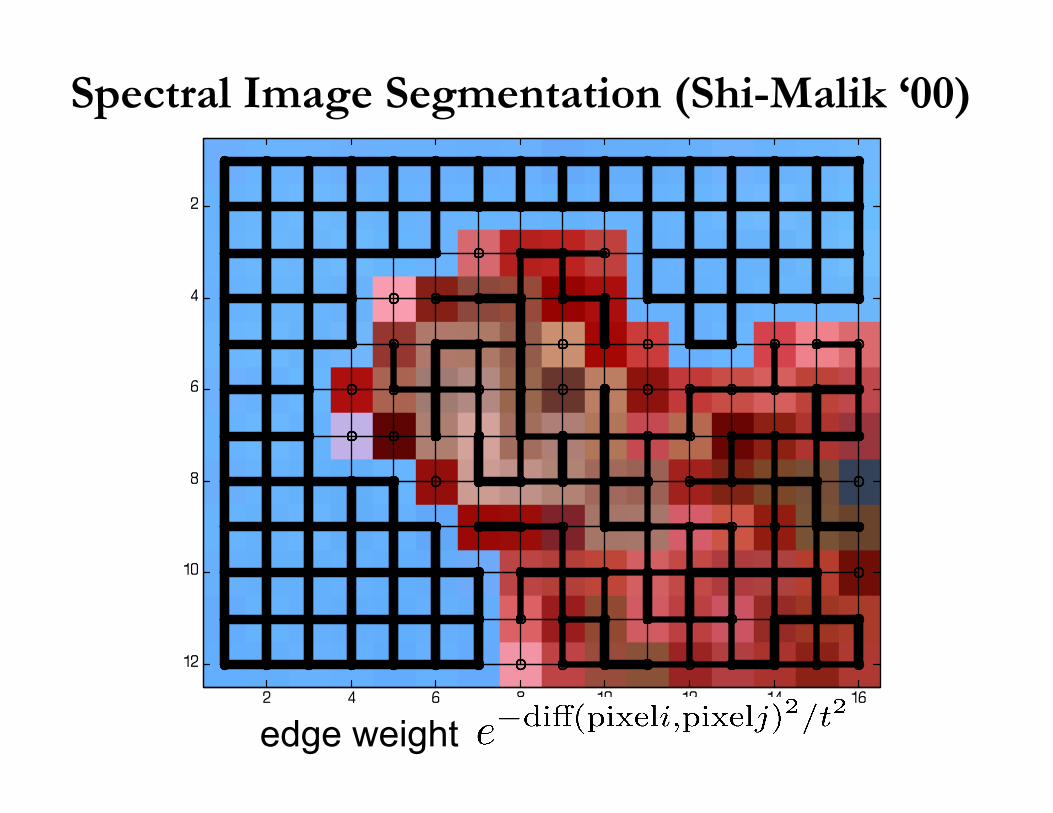
Spectral Image Segmentation (Shi-Malik ‘00)

Spectral Image Segmentation (Shi-Malik ‘00)

Spectral Image Segmentation (Shi-Malik ‘00)

Spectral Image Segmentation (Shi-Malik ‘00)
Spectral Image Segmentation (Shi-Malik ‘00)
edge weight

The second eigenvector

Second eigenvector cut
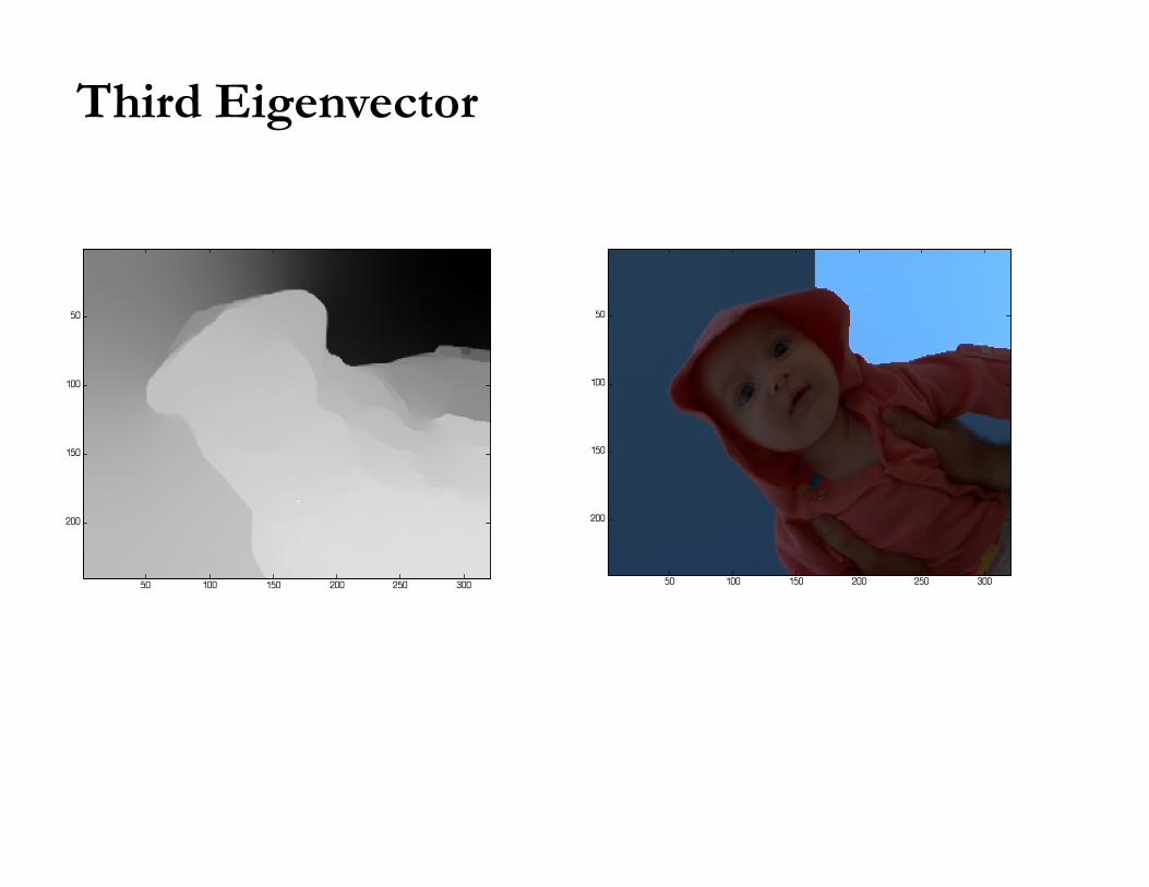
Third Eigenvector

Fourth Eigenvector

Cheeger’s Inequality [Alon-Milman ‘85, Jerrum-Sinclair ‘89, Diaconis-Stroock ‘91]
[Cheeger ‘70]
For Normalized Laplacian: L = D−1/2LD−1/2
And, is a spectral cut for which
λ2/2 ≤ minS
Φ(S) ≤�2λ2
Φ(S) ≤�2λ2
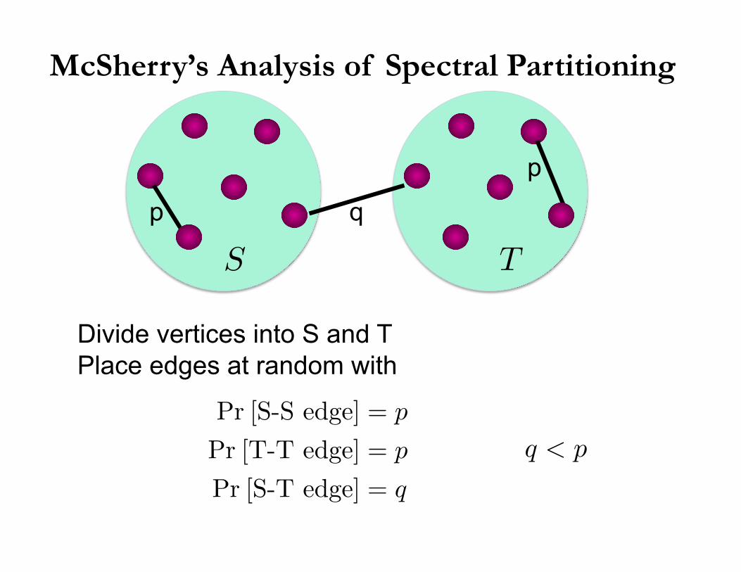
McSherry’s Analysis of Spectral Partitioning
S T
p
p
q
Divide vertices into S and T Place edges at random with
Pr [S-S edge] = p
Pr [T-T edge] = p
Pr [S-T edge] = q
q < p
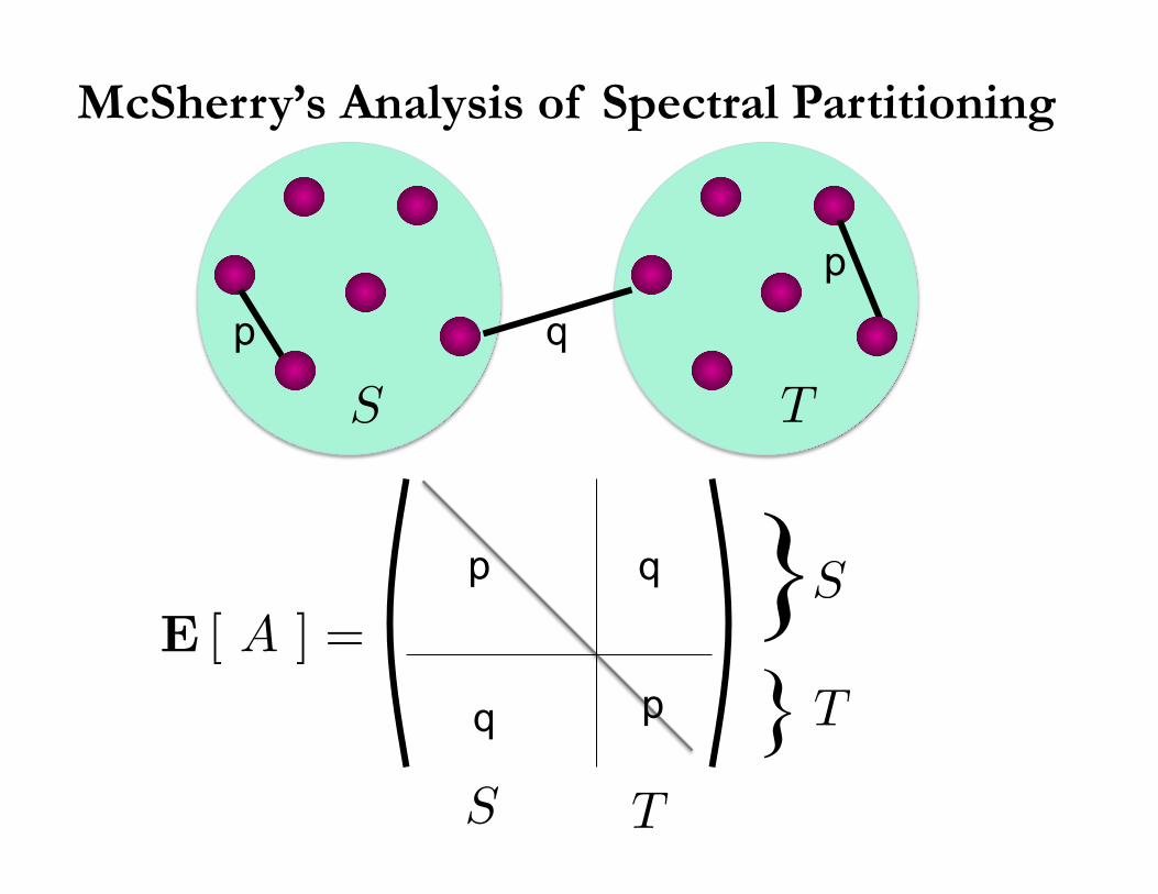
McSherry’s Analysis of Spectral Partitioning
S T
p
p
q
E [ A ] =
p q
q p
}} T
TS
S
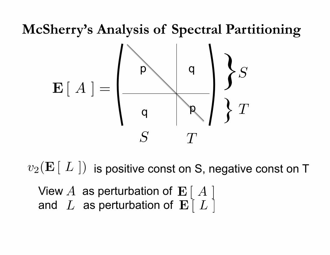
McSherry’s Analysis of Spectral Partitioning
E [ A ] =
p q
q p
}} T
TS
S
is positive const on S, negative const on T
View as perturbation of and as perturbation of E [ L ]
E [ A ]AL
v2(E [ L ])
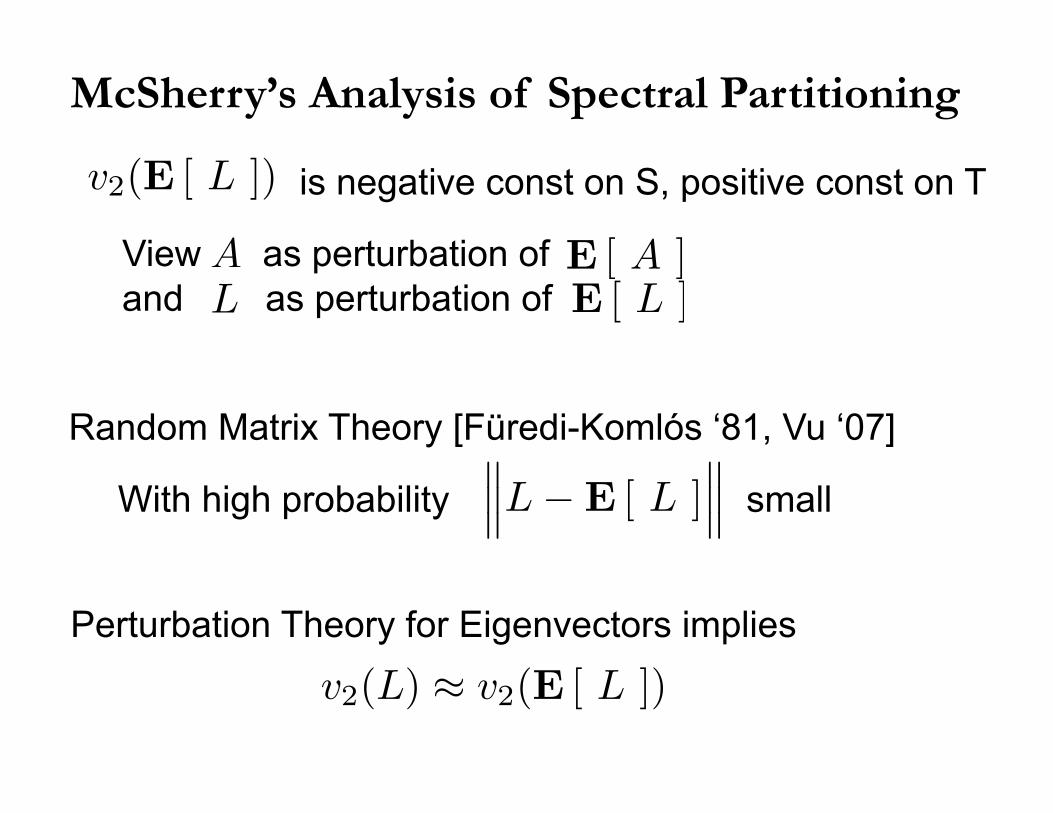
is negative const on S, positive const on T
McSherry’s Analysis of Spectral Partitioning
View as perturbation of and as perturbation of E [ L ]
E [ A ]AL
Random Matrix Theory [Füredi-Komlós ‘81, Vu ‘07]
With high probability small ���L−E [ L ]
���
Perturbation Theory for Eigenvectors implies
v2(L) ≈ v2(E [ L ])
v2(E [ L ])

Spectral graph coloring from high eigenvectors
Embedding of dodecahedron by 19th and 20th eigvecs.

Spectral graph coloring from high eigenvectors
Coloring 3-colorable random graphs [Alon-Kahale ’97]
p
pp
p
p
Independent Sets
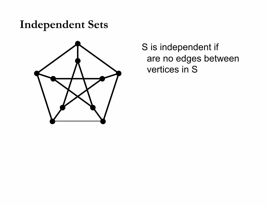
S is independent if are no edges between vertices in S

Independent Sets
S is independent if are no edges between vertices in S
Hoffman’s Bound: if every vertex has degree d
|S| ≤ n
�1− d
λn
�
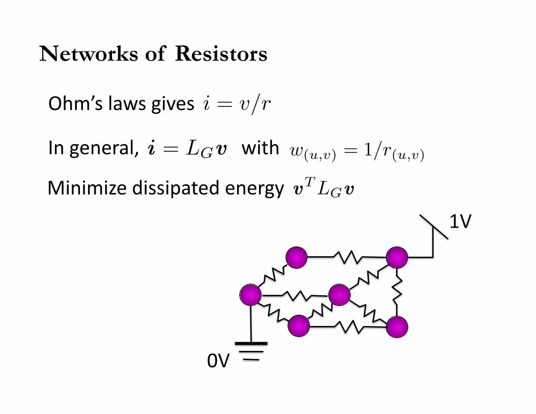
Networks of Resistors
Ohm’s laws gives
In general, with w(u,v) = 1/r(u,v)
Minimize dissipated energy
i = v/r
i = LGv
vTLGv
1V
0V
1V
0V
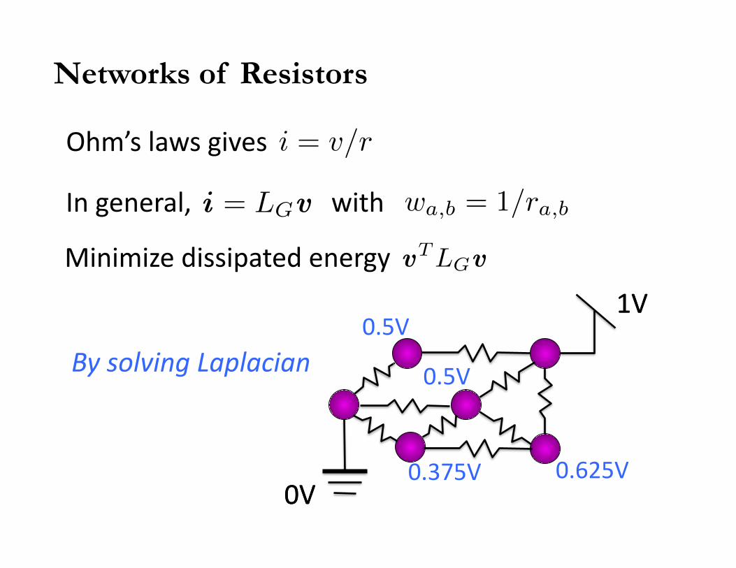
0.5V
0.5V
0.625V 0.375V
By solving Laplacian
1V
0V
Ohm’s laws gives
In general, with
Minimize dissipated energy
i = v/r
i = LGv
vTLGv
Networks of Resistors
wa,b = 1/ra,b
Electrical Graph Theory
Considers flows in graphs
Allows comparisons of graphs, and embedding of one graph within another.
Relative Spectral Graph Theory

Effective Resistance
Resistance of entire network, measured between a and b.
= 1/(current flow at one volt)
0V
0.53V
0.27V
0.33V 0.2V
1V
0V
a b
Ohm’s law:
Reff(a, b)
r = v/i

Effective Resistance
= 1/(current flow at one volt) = voltage difference to flow 1 unit
Ohm’s law:
Reff(a, b)
Resistance of entire network, measured between a and b.
r = v/i
Effective Resistance
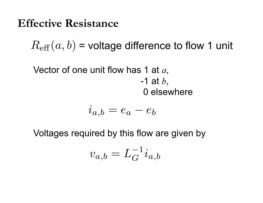
= voltage difference to flow 1 unit Reff(a, b)
ia,b = ea − eb
Vector of one unit flow has 1 at a, -1 at b, 0 elsewhere
Voltages required by this flow are given by
va,b = L−1G ia,b
Effective Resistance
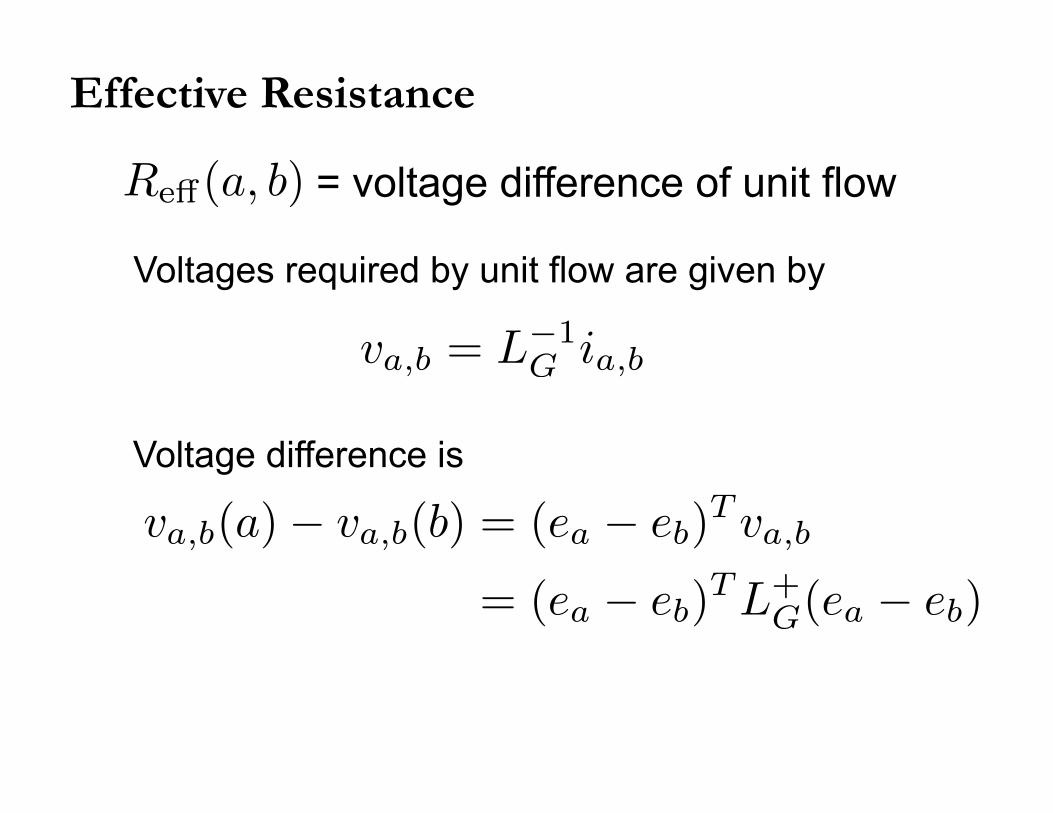
= voltage difference of unit flow Reff(a, b)
Voltages required by unit flow are given by
Voltage difference is
va,b(a)− va,b(b) = (ea − eb)T va,b
= (ea − eb)TL+
G(ea − eb)
va,b = L−1G ia,b
Effective Resistance Distance
Effective resistance is a distance Lower when are more short paths
Equivalent to commute time distance: expected time for a random walk from a to reach b and then return to a.
See Doyle and Snell, Random Walks and Electrical Networks

Relative Spectral Graph Theory
For two connected graphs G and H with the same vertex set, consider
LGL−1H
work orthogonal to nullspace or use pseudoinverse
Allows one to compare G and H
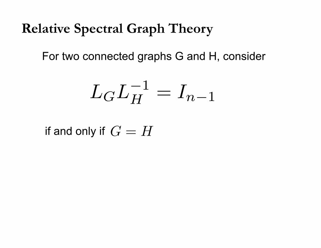
Relative Spectral Graph Theory
For two connected graphs G and H, consider
if and only if G = H
LGL−1H
= In−1
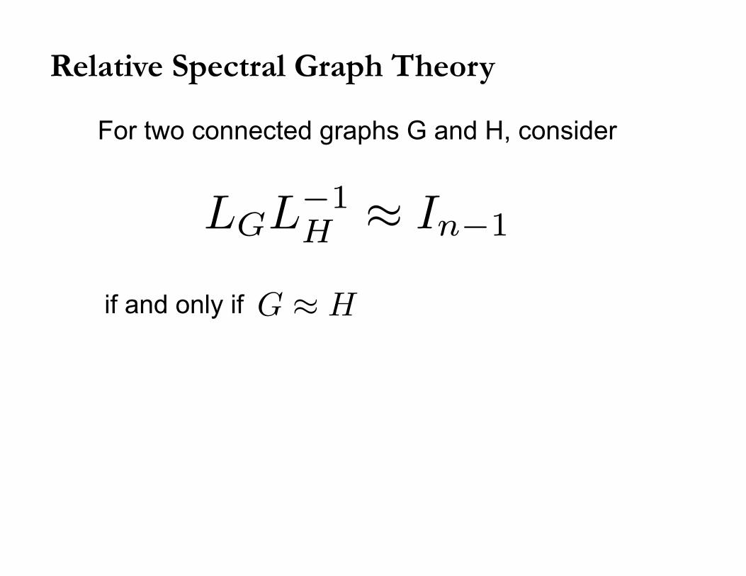
Relative Spectral Graph Theory
For two connected graphs G and H, consider
if and only if
LGL−1H
≈ In−1
G ≈ H
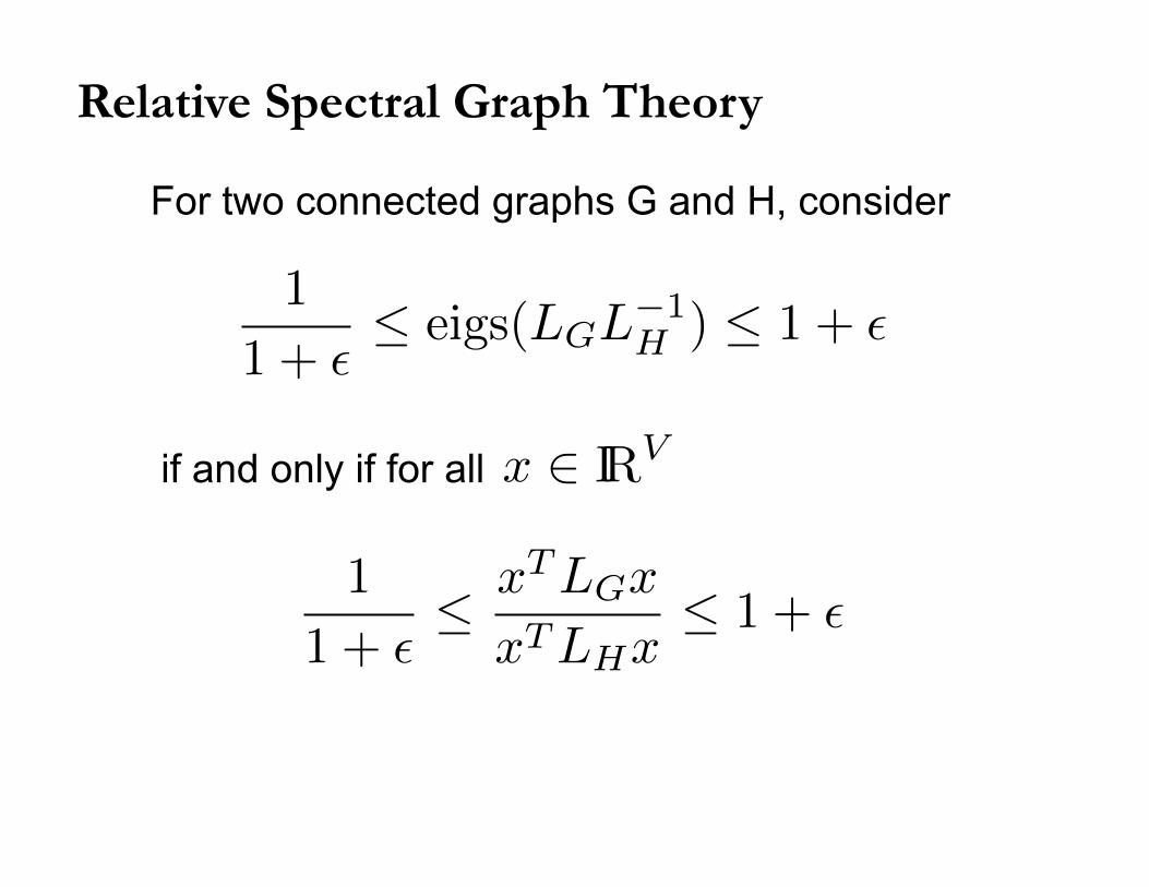
Relative Spectral Graph Theory
For two connected graphs G and H, consider
if and only if for all
1
1 + �≤ eigs(LGL
−1H
) ≤ 1 + �
1
1 + �≤ xTLGx
xTLHx≤ 1 + �
x ∈ IRV
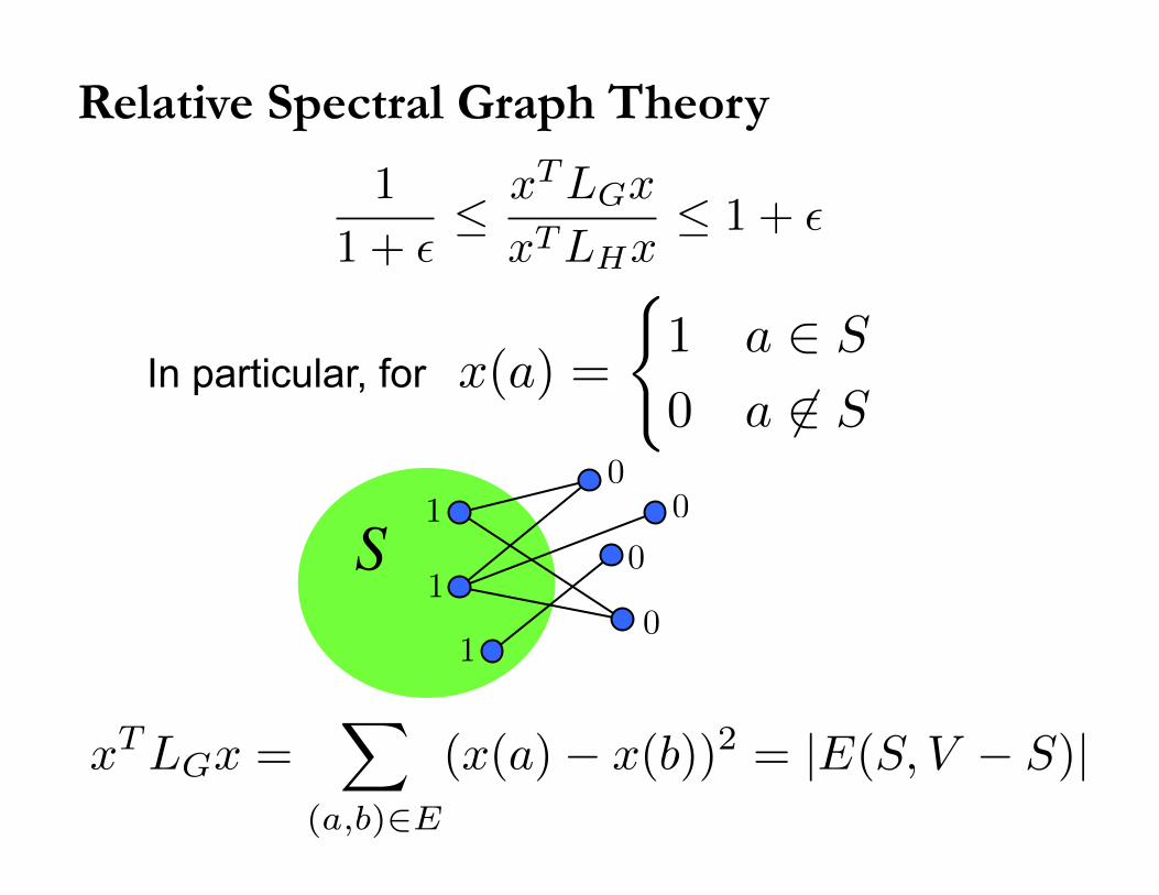
xTLGx =�
(a,b)∈E
(x(a)− x(b))2 = |E(S, V − S)|
Relative Spectral Graph Theory
1
1 + �≤ xTLGx
xTLHx≤ 1 + �
In particular, for
00
0
1
1
1
S 0
x(a) =
�1 a ∈ S
0 a �∈ S

Relative Spectral Graph Theory
For all
1
1 + �≤ |EG(S, V − S)|
|EH(S, V − S)| ≤ 1 + �
S ⊂ V
1
1 + �≤ xTLGx
xTLHx≤ 1 + �

Expanders Approximate Complete Graphs
Expanders:
d-regular graphs on n vertices
high conductance
random walks mix quickly
weak expanders: eigenvalues bounded from 0
strong expanders: all eigenvalues near d
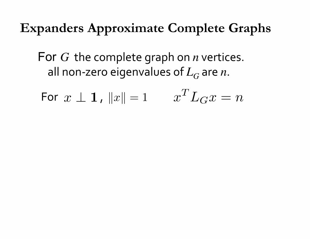
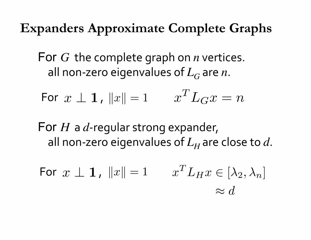
For G the complete graph on n vertices. all non-‐zero eigenvalues of LG are n.
For , x ⊥ 1 xTLGx = n�x� = 1
Expanders Approximate Complete Graphs
For G the complete graph on n vertices. all non-‐zero eigenvalues of LG are n.
For , x ⊥ 1 xTLGx = n
For H a d-‐regular strong expander, all non-‐zero eigenvalues of LH are close to d.
For , x ⊥ 1
�x� = 1
�x� = 1
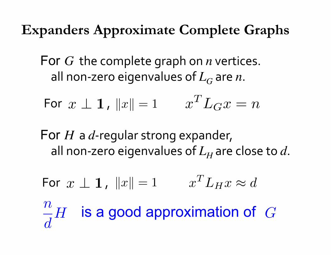
Expanders Approximate Complete Graphs
xTLHx ∈ [λ2,λn]
≈ d
For , x ⊥ 1
n
dH is a good approximation of G
�x� = 1
Expanders Approximate Complete Graphs
xTLHx ≈ d
For G the complete graph on n vertices. all non-‐zero eigenvalues of LG are n.
For , x ⊥ 1 xTLGx = n
For H a d-‐regular strong expander, all non-‐zero eigenvalues of LH are close to d.
�x� = 1

Sparse approximations of every graph
Can find an H with edges in nearly-linear time.
O(n log n/�2)
[Batson-S-Srivastava]
[S-Srivastava]
1
1 + �≤ xTLGx
xTLHx≤ 1 + �
For every G, there is an H with edges (2 + �)2n/�2
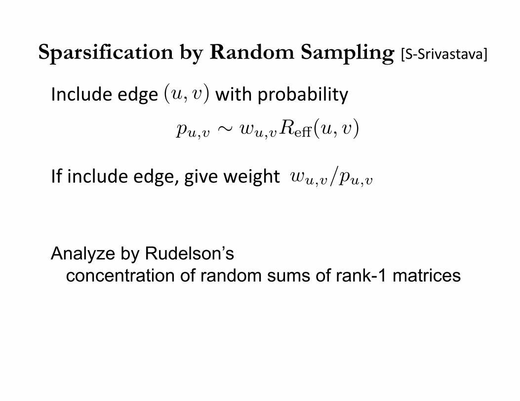
Sparsification by Random Sampling [S-‐Srivastava]
Include edge with probability (u, v)
pu,v ∼ wu,vReff(u, v)
If include edge, give weight wu,v/pu,v
Analyze by Rudelson’s concentration of random sums of rank-1 matrices
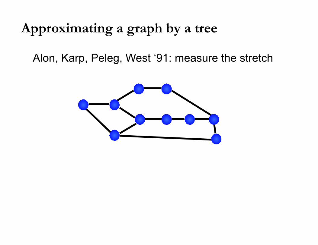
Approximating a graph by a tree
Alon, Karp, Peleg, West ‘91: measure the stretch
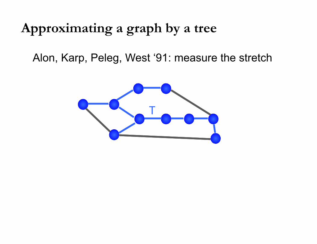
T
Approximating a graph by a tree
Alon, Karp, Peleg, West ‘91: measure the stretch
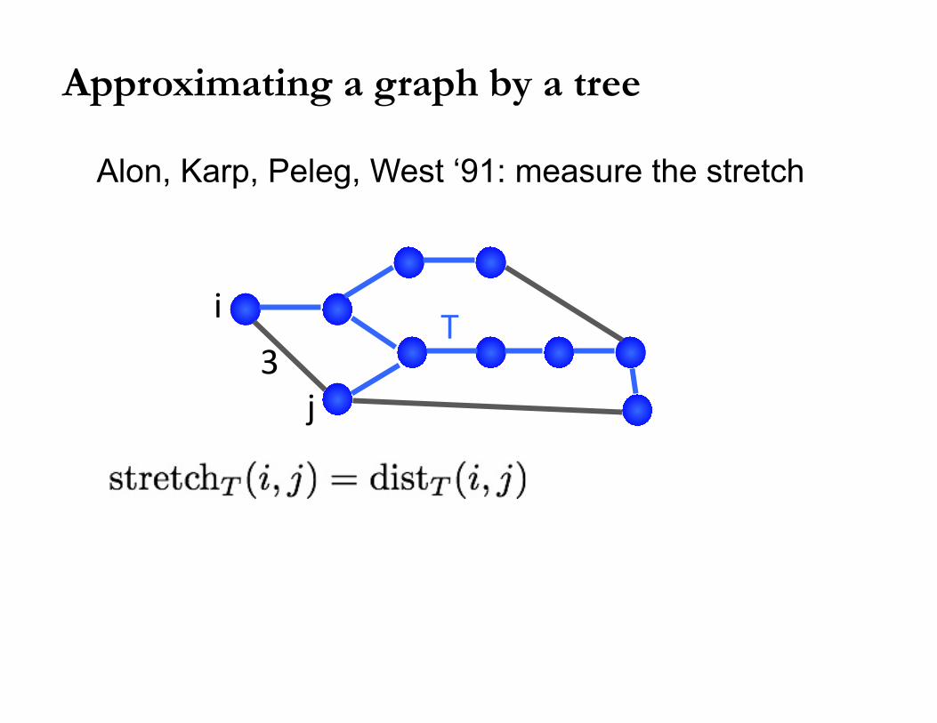
i
j 3
T
Approximating a graph by a tree
Alon, Karp, Peleg, West ‘91: measure the stretch
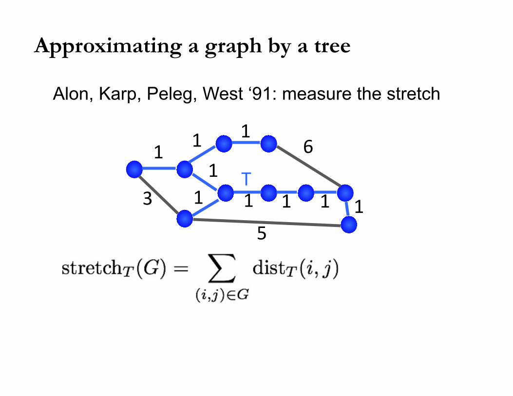
T 3
5
6 1 1
1 1
1 1 1 1 1
Approximating a graph by a tree
Alon, Karp, Peleg, West ‘91: measure the stretch
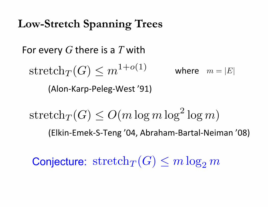
(Alon-‐Karp-‐Peleg-‐West ’91)
(Elkin-‐Emek-‐S-‐Teng ’04, Abraham-‐Bartal-‐Neiman ’08)
For every G there is a T with
where m = |E|
Low-Stretch Spanning Trees
Conjecture:
stretchT (G) ≤ m1+o(1)
stretchT (G) ≤ O(m logm log2 logm)
stretchT (G) ≤ m log2 m
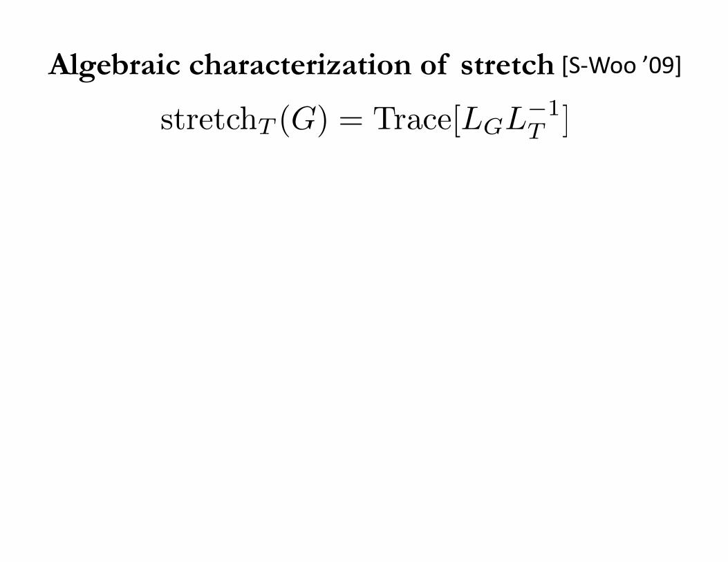
[S-‐Woo ’09] Algebraic characterization of stretch
stretchT (G) = Trace[LGL−1T ]

In trees, resistance is distance.
Resistances in series sum
[S-‐Woo ’09] Algebraic characterization of stretch
T a b
v : 0 11 1
2
2
3 44
4
stretchT (G) = Trace[LGL−1T ]
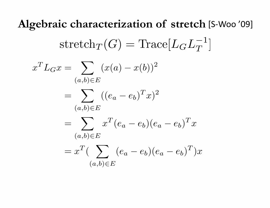
xTLGx =�
(a,b)∈E
(x(a)− x(b))2
=�
(a,b)∈E
((ea − eb)Tx)2
=�
(a,b)∈E
xT (ea − eb)(ea − eb)Tx
= xT (�
(a,b)∈E
(ea − eb)(ea − eb)T )x
[S-‐Woo ’09] Algebraic characterization of stretch
stretchT (G) = Trace[LGL−1T ]
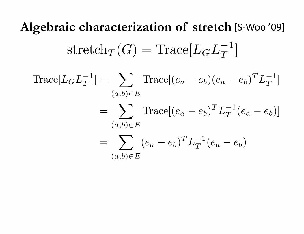
[S-‐Woo ’09] Algebraic characterization of stretch
stretchT (G) = Trace[LGL−1T ]
Trace[LGL−1T ] =
�
(a,b)∈E
Trace[(ea − eb)(ea − eb)TL−1
T ]
=�
(a,b)∈E
Trace[(ea − eb)TL−1
T (ea − eb)]
=�
(a,b)∈E
(ea − eb)TL−1
T (ea − eb)

[S-‐Woo ’09] Algebraic characterization of stretch
stretchT (G) = Trace[LGL−1T ]
�
(a,b)∈E
(ea − eb)TL−1
T (ea − eb) =�
(a,b)∈E
Reff(a, b)
=�
(a,b)∈E
stretchT (a, b)

Notable Things I’ve left out
Behavior under graph transformations Graph Isomorphism Random Walks and Diffusion PageRank and Hits Matrix-Tree Theorem Special Graphs (Cayley, Strongly-Regular, etc.) Diameter bounds Colin de Verdière invariant Discretizations of Manifolds
The next two talks
Tomorrow: Solving equations in Laplacians in nearly-linear time.
Preconditioning Sparsification Low-Stretch Spanning Trees Local graph partitioning
The next two talks
Thursday: Existence of sparse approximations.
A theorem in linear algebra and some of its connections.