spectral broadening caused by dynamic speckle in self-mixing

Spectral broadening caused by dynamicspeckle in self-mixing velocimetry

sensors

Russell Kliese and A. D. Rakic∗The University of Queensland, School of Information Technology and Electrical Engineering,

Brisbane, QLD 4072, Australia∗[email protected]

Abstract: Self-mixing laser sensors require few components and can beused to measure velocity. The self-mixing laser sensor consists of a laseremitting a beam focused onto a rough target that scatters the beam withsome of the emission re-entering the laser cavity. This ‘self-mixing’ causesmeasurable interferometric modulation of the laser output power that leadsto a periodic Doppler signal spectrum with a peak at a frequency propor-tional to the velocity of the target. Scattering of the laser emission froma rough surface also leads to a speckle effect that modulates the Dopplersignal causing broadening of the signal spectrum adding uncertainty to thevelocity measurement. This article analyzes the speckle effect to providean analytic equation to predict the spectral broadening of an acquiredself-mixing signal and compares the predicted broadening to experimentalresults. To the best of our knowledge, the model proposed in this articleis the first model that has successfully predicted speckle broadening in aself-mixing velocimetry sensor in a quantitative manner. It was found thatthe beam spot size on the target and the target speed affect the resultingspectral broadening caused by speckle. It was also found that the broadeningis only weakly dependent on target angle. The experimental broadening wasconsistently greater than the theoretical speckle broadening due to othereffects that also contribute to the total broadening.

© 2012 Optical Society of America

OCIS codes: (280.3340) Laser Doppler velocimetry; (030.6140) Speckle; (030.6600) Statisti-cal optics; (250.7260) Vertical cavity surface emitting lasers.

References and links1. R. Lang and K. Kobayashi, “External optical feedback effects on semiconductor injection laser properties,” IEEE

J. Quantum Electron. QE-16, 347–355 (1980).2. Y. Mitsuhashi, J. Shimada, and S. Mitsutsuka, “Voltage change across the self-coupled semiconductor laser.”

IEEE J. Quantum Electron. QE-17, 1216–1225 (1981).3. J. H. Churnside, “Laser Doppler velocimetry by modulating a CO2 laser with backscattered light,” Appl. Opt.

23, 61–66 (1984).4. S. Shinohara, A. Mochizuki, H. Yoshida, and M. Sumi, “Laser Doppler velocimeter using the self-mixing effect

of a semiconductor laser diode,” Appl. Opt. 25, 1417–1419 (1986).5. M. Rudd, “A laser Doppler velocimeter employing the laser as a mixer-oscillator,” J. Phys. E 1, 723–726 (1968).6. G. Giuliani, M. Norgia, S. Donati, and T. Bosch, “Laser diode self-mixing technique for sensing applications,” J.

Opt. A Pure Appl. Opt. 4, 283–294 (2002).7. L. E. Estes, L. M. Narducci, and R. A. Tuft, “Scattering of light from a rotating ground glass,” J. Opt. Soc. Am.

61, 1301–1306 (1971).

#168214 - $15.00 USD Received 8 May 2012; revised 12 Jun 2012; accepted 20 Jul 2012; published 1 Aug 2012(C) 2012 OSA 13 August 2012 / Vol. 20, No. 17 / OPTICS EXPRESS 18757

8. N. Takai, “Statistics of dynamic speckles produced by a moving diffuser under the Gaussian beam laser illumi-nation,” Jpn. J. Appl. Phys. 13, 2025–2032 (1974).

9. E. Jakeman, “The effect of wavefront curvature on the coherence properties of laser light scattered by targetcentres in uniform motion,” J. Phys. A 8, L23–L28 (1975).

10. B. E. A. Saleh, “Speckle correlation measurement of the velocity of a small rotating rough object,” Appl. Opt.14, 2344–2346 (1975).

11. P. N. Pusey, “Photon correlation study of laser speckle produced by a moving rough surface,” J. Phys. D 9,1399–1409 (1976).

12. H. Jentink, F. de Mul, H. Suichies, J. Aarnoudse, and J. Greve, “Small laser Doppler velocimeter based on theself-mixing effect in a diode laser,” Appl. Opt. 27, 379–385 (1988).

13. Sahin Kaya Ozdemir, T. Takasu, S. Shinohara, H. Yoshida, and M. Sumi, “Simultaneous measurement of velocityand length of moving surfaces by a speckle velocimeter with two self-mixing laser diodes,” Appl. Opt. 38, 1968–1974 (1999).

14. X. Raoul, T. Bosch, G. Plantier, and N. Servagent, “A double-laser diode onboard sensor for velocity measure-ments,” IEEE Trans. Instr. Meas. 53, 95–101 (2004).

15. R.-H. Hage, T. Bosch, G. Plantier, and A. Sourice, “Modeling and analysis of speckle effects for velocitymeasurements with self-mixing laser diode sensors,” in Sensors, 2008 IEEE (IEEE, 2008), 953–956.

16. D. Han, S. Chen, and L. Ma, “Autocorrelation of self-mixing speckle in an EDFR laser and velocity measure-ment,” Appl. Phys. B 103, 695–700 (2011).

17. H. Wang, J. Shen, B. Wang, B. Yu, and Y. Xu, “Laser diode feedback interferometry in flowing Brownian motionsystem: a novel theory,” Appl. Phys. B 101, 173–183 (2010).

18. J. W. Goodman, “Statistical properties of laser speckle patterns,” in Laser Speckle and Related Phenomena, J. C.Dainty, ed. (Springer-Verlag, 1975), chap. 2.

19. J. W. Goodman, Statistical Optics (John Wiley & Sons, 1985).20. G. Giuliani and M. Norgia, “Laser diode linewidth measurement by means of self-mixing interferometry,” IEEE

Photon. Technol. Lett. 12, 1028–1030 (2000).21. A. Papoulis and S. U. Pillai, “Stochastic processes: General concepts,” in Probability, Random Variables, and

Stochastic Processes (McGraw Hill, 2002), chap. 9, 4th ed.22. J. W. Goodman, “Fresnel and Fraunhofer diffraction,” in Introduction to Fourier Optics (Roberts & Company,

2005), chap. 4, 3rd ed.23. J. W. Goodman, “Effects of partial coherence on imaging systems,” in Statistical Optics (John Wiley & Sons,

1985), chap. 7.24. R. Juskaitis, N. Rea, and T. Wilson, “Semiconductor laser confocal microscopy,” Appl. Opt. 33, 578–584 (1994).25. H. Albrecht, M. Borys, N. Damaschke, and C. Tropea, Laser Doppler and Phase Doppler Measurement Tech-

niques (Springer Verlag, 2003).26. R. S. Matharu, J. Perchoux, R. Kliese, Y. L. Lim, and A. D. Rakic, “Maintaining maximum signal-to-noise ratio

in uncooled vertical-cavity surface-emitting laser-based self-mixing sensors,” Opt. Lett. 36, 3690–3692 (2011).27. J. Scott, R. Geels, S. Corzine, and L. Coldren, “Modeling temperature effects and spatial hole burning to optimize

vertical-cavity surface-emitting laser performance,” IEEE J. Quantum Electron. 29, 1295–1308 (1993).28. J. W. Goodman, “Random processes,” in Statistical Optics (John Wiley & Sons, 1985), chap. 3.29. D. Middleton, “Spectra, covariance, and correlation functions,” in An Introduction to Statistical Communication

Theory (IEEE Press, 1996), chap. 3. Reprint.30. D. Middleton, “Statistical preliminaries,” in An Introduction to Statistical Communication Theory (IEEE Press,

1996), chap. 1. Reprint.31. Y. Suzaki and A. Tachibana, “Measurement of the µm sized radius of Gaussian laser beam using the scanning

knife-edge,” Appl. Opt. 14, 2809–2810 (1975).32. J. M. Khosrofian and B. A. Garetz, “Measurement of a Gaussian laser beam diameter through the direct inversion

of knife-edge data,” Appl. Opt. 22, 3406–3410 (1983).33. R. N. Bracewell, “The basic theorems,” in The Fourier Transform and Its Applications (McGraw Hill, 2000),

chap. 6.34. J. W. Goodman, Introduction to Fourier Optics (Roberts & Company, 2005), 3rd ed.35. B. E. A. Saleh and M. C. Teich, “Beam optics,” in Fundamentals of Photonics (Wiley, 2007), chap. 3, 2nd ed.

1. Introduction

Simple sensors can be built using semiconductor lasers when a portion of the light emittedre-enters the laser cavity causing measurable changes in the emitted power [1] and the laserterminal voltage [2]. Such ‘self-mixing’ sensors can be used to measure the speed of a roughmoving target [3, 4]. Light scattered by a target with a velocity component parallel to the laseremission axis experiences a Doppler shift. The self-mixing sensor acts as a homodyne sys-


tem [5] whereby the Doppler shift in the reflected light leads to a periodic self-mixing signal(either acquired directly from the laser terminal voltage variations or from a photodetector thatsenses the variations in the optical power [4]).

Unlike a smooth surface, a rough surface makes it possible for the target to be inclined at anyangle; it need not be aligned normal to the emission axis because a rough surface causes lightto be scattered in all directions. An ideal self-mixing Doppler signal, in the absence of speckleeffect, would be a harmonic function with a constant amplitude; in the frequency domain itwould be represented by a single spectral line. However, a rough surface leads to a dynamicspeckle effect causing the self-mixing Doppler signal to exhibit variations in amplitude [6] andphase. This leads to spectral broadening in the frequency domain [3].

Spectral broadening due to the dynamic speckle effect has been reported since the 1970’s [7–11]. However, the literature pertaining to the effect in self-mixing sensors is more limited.The dynamic speckle effect in self-mixing sensors has been experimentally reported by severalgroups [12–14], and a number of models have been proposed [15,16] including a model for themore complex problem of fluid flow with Brownian motion [17].

To the best of our knowledge, this article reports for the first time a model that has success-fully predicted speckle broadening in a self-mixing velocimetry sensor in a qualitative mannerthat has been validated by experimental results. The model requires no parameter fitting beingentirely based on the underlying optical physics of the speckle effect.

This article investigates the statistical properties of dynamic speckle from rough surfacesallowing the broadening to be predicted for given system parameters. It builds on the statis-tical optics foundations of Goodman [18, 19] and dynamic speckle theory published by Esteset al. [7], Jakeman [9], and Pusey [11]. The speckle model developed here applies to the self-mixing velocimetry sensor where a laser spot with Gaussian profile is focused onto the target.We show that smaller spot sizes lead to increased spectral broadening; this is particularly im-portant for high spatial resolution sensors that make use of small laser spots. Broadening of thesignal leads to uncertainty in the velocity obtained from the sensor.

Experimental verification of the speckle statistics is provided; the results are based onVertical-Cavity Surface-Emitting Lasers (VCSELs) that are particularly well suited to self-mixing sensing applications. They typically have low threshold currents, often below one mil-liampere, making them suitable for mobile applications. They also often have an approximatelycircular, anastigmatic beam and Gaussian beam profile making optical design simpler than foredge emitting devices whose beam is elliptical and frequently astigmatic. VCSELs are alsoavailable at a low cost because of their mass production for short-haul communication linksand computer mouse devices.

Apart from the speckle effect, there are several other factors that contribute to the Dopplerline broadening. Firstly, a range of velocities is present over the illuminated spot region on a ro-tating target. This effect becomes more pronounced with the increased gradient in the velocitydistribution that occurs closer to the axis of rotation. Secondly, the vibration and surface profilevariation of the target adds an additional component to an otherwise constant velocity. Finally,the finite linewidth of the laser emission adds uncertainty to the fringe locations of self-mixingsignals [20]. In order to concentrate this paper on speckle broadening effects alone, experimen-tal parameters were chosen to minimize these additional sources of broadening where possible.The additional sources of broadening will be the topic of a subsequent publication.

In Sec. 2 the key results from the derivation of the Doppler signal broadening caused bythe dynamic speckle effect are presented with the full derivation left to appendix A. Section 3presents the relevant laser characteristics measured for the two lasers used in the experimentalvalidation (with some additional details relating to the measurement of the VCSEL beam waistradius left to appendix B). Section 4 then compares the experimental results to the theory for


target with a rough

surface at beam waist

v

θ

incoming beam

x

y

P

ξ

η

z

Fig. 1. Geometry used for the derivation of the dynamic speckle statistics at point P. A fieldwhich has the x,y coordinate system is incident on the rough surface moving with velocityv which is inclined at an angle θ from the x axis. This field is scattered by the rough surfaceand the resulting time autocorrelation function of the field at P with coordinates ξ ,η isderived.

a range of target speeds, a range of spot sizes, and a range of target angles. This is followed byconcluding remarks.

2. Statistical properties of speckle fields

In this section, the theory necessary to obtain the statistical properties of the light coupled backinto the self-mixing sensor is presented so that an equation for the dynamic speckle broadeningcan be formulated. The statistical autocorrelation function for differences between observationstimes of the field at a point is presented (the full derivation is left to appendix A). The powerspectral density of the self-mixing signal can then be obtained from the Fourier transform ofthe autocorrelation function [21] which can be directly compared to experimentally obtainedpower spectral densities of the self-mixing signal.

This analysis considers the case where the laser is focused on the target to be measured.The maximum power is coupled back into the laser under this condition, leading to the bestsignal-to-noise ratio (SNR); this is the configuration most used in practice. Figure 1 showsthe geometry and coordinate systems used to derive the statistical autocorrelation function forthe field at point P. The laser beam enters from the right and is focused onto a spot on thetarget which has a rough surface. The rough surface scatters the incident light producing aspeckle field in the ξ -η plane. Point P is the point on the laser emission axis at a distancez from the target sufficient that the Fresnel approximations can be used to calculate the fieldin the ξ -η plane using the Fresnel diffraction integral. (The sufficient conditions for accuracyof the Fresnel approximation are complicated [22], but the distance z will be sufficient if P isconsidered to be just in front of the focusing lens discussed in Sec. 4.) Point P is the point wherethe coupling between the incoming field and the speckle field is obtained.

2.1. Assumptions

Several assumptions were used to simplify the problem and allow an analytic solution for thepower spectral density to be obtained. These assumptions are:

1. The target is rough compared to the wavelength of illumination so that the reflectedlight from each point undergoes several 2π phase shifts before arriving at a phase that isuniformly distributed on the interval (−π,π]. This condition is satisfied by the majorityof man-made and natural surfaces [23].


2. The microstructure of the scattering surface is finer than the resolving power of an aper-ture at point P with a diameter of the order of the beam waist diameter. This assumptionof fine microstructure allows the spatial autocorrelation function of the target to be wellapproximated by a delta function [18].

3. The spatial extent of the spot is sufficient so that a large number of individual scatteringsites are illuminated.

4. The laser emission is monochromatic.

5. Only one polarization is considered and depolarization effects are ignored. This assump-tion makes the derivation of the model tractable.

6. The speckle grain size is sufficiently large so that the field variation over the illuminatedregion at P is insignificant (the speckle grain will have a linear dimension of the order ofλ z/r where λ is the laser emission wavelength and r is the spot radius [7]).

7. The wave-fronts of the incoming beam and the scattered beam at P have identical curva-ture. The spherical scattered field will approximate the incoming field on the axis whenfocused to a small spot on the target.

8. The change in intensity at point P is proportional to the change in the laser terminal volt-age. This is valid for the weak feedback regime used in the experiments. The equivalencebetween the intensity and the laser terminal voltage variation has been demonstrated ex-perimentally [4] and is supported by a theoretical model [24].

2.2. Statistical time-autocorrelation function

In this section we present the autocorrelation function for the field at P. The field at P will havea Gaussian probability distribution by the central limit theorem because it is the sum of manyindependent random variables: the components from many different scatterers on the rough sur-face. Therefore, the autocorrelation function and mean completely describe the random process.Furthermore, the mean is zero (see Appendix A).

The statistical autocorrelation function of the field amplitude RA, at P as a function of thedifference between observation times τ , is:

RA(τ) =exp

(i 4πvτ sinθ

λ)

λ 2z2

∫∫ ∞

−∞U(x+ vτ cosθ ,y)U∗(x,y)

× exp

⎧⎨

⎩

iπ[(x+ vτ cosθ)2 − x2

]

λ z

⎫⎬

⎭dxdy . (1)

where λ is the wavelength of the laser emission, θ is the inclination angle of the target, U isthe field incident on the rough surface, ∗ denotes the complex conjugate, and i is the imaginaryunit (

√−1).Surface profile parameters are absent from Eq. (1) due to assumption 1 in Sec. 2.1. This

Independence of broadening on surface microstructure has been validated experimentally bymeasuring the broadening from a sand-blasted aluminum surface and from a paper surface.Under a range of conditions, the broadenings obtained from both surfaces were identical.

VCSELs used for self-mixing sensors often have emission profiles that are approximatelyGaussian. An analytic result can be obtained for the autocorrelation function for the specific


0

0.5

1

2vsinθλ

S A(

f)

f

vcosθ√

2loge 2

πwt

Fig. 2. A plot of the normalised power spectral density with the FWHM and peak frequencyindicated.

case of Gaussian illumination specified by the beam waist radius at the target wt . If the Gaussianfield,

UG(x,y) =2

πw2t

exp

(−x2 + y2

w2t

), (2)

is substituted into Eq. (1), the normalised power spectral density can be obtained as a functionof frequency f ,

SA( f ) = exp

[

−2π2w2t ( f − 2vsinθ

λ )2

v2

]

. (3)

This result makes use of an approximation valid for small spot sizes (see Sec. 6.1 in appendixA for details). In this work, the spectral broadening is quantified by measuring the full-widthhalf-maximum (FWHM) of the Doppler signals. The FWHM of Eq. (3) is:

FWHM =vcosθ

√2loge 2

πwt. (4)

The peak frequency fD, is the parameter used to obtain the target velocity in self-mixing ve-locimetry sensors and is given by:

fD =2vsinθ

λ, (5)

which is in agreement with the Doppler frequency from [25].A plot of SA( f ), with the FWHM and peak labeled, appears in Fig. 2. The simple analytic

formula for the FWHM can be used to predict spectral broadening for self-mixing sensors.This result shows that the speckle broadening of Doppler self-mixing signal depends only onthe component of the target velocity normal to the optical axis and the beam waist radius onthe target. Notably it does not depend explicitly on wavelength, and is independent of the targetinclination angle in the small angle approximation.

3. Laser characterization

In order to validate the dynamic speckle theory, we wanted to choose representative lasersused for self-mixing interferometry. In order to simplify the analysis, we limited the choiceof lasers to VCSELs operating in a single transverse mode, which is typically obtained fromdevices with small apertures. We chose two mass produced VCSELs, one with visible emission(Firecomms, RVM665T) and one with infra-red emission (Litrax, LX-VCS-850-T311), withnominal emission wavelengths of 665 nm and 850 nm respectively. All measurements weremade at room temperature of approximately 25°C.


0.0

0.5

1.0

1.5

0 1 2 3 4 5 6 7

op

tica

lp

ow

er(a

.u.)

current (mA)

0.90 mA

(a)

0.0

0.5

1.0

1.5

2.0

2.5

3.0

0 5 10 15 20

op

tica

lp

ow

er(a

.u.)

current (mA)

3.0 mA

(b)

667 668 669

inte

nsi

ty(a

.u.)

wavelength (nm)

851 852

inte

nsi

ty(a

.u.)

wavelength (nm)

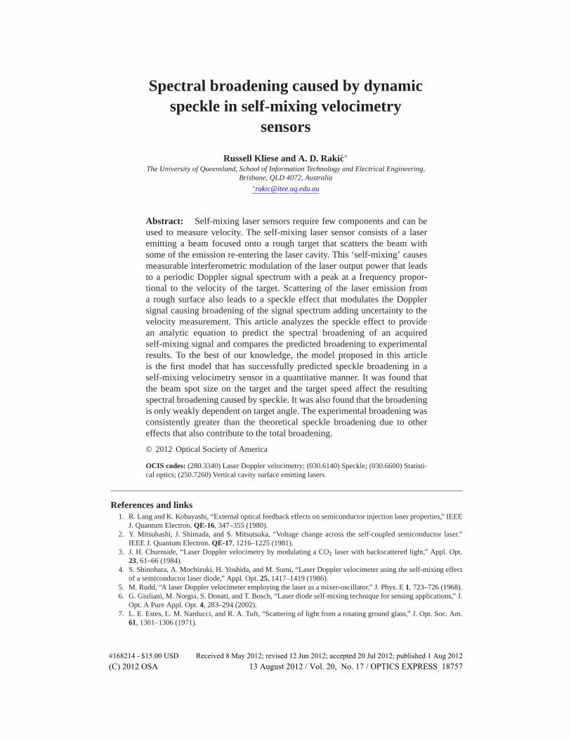
Fig. 3. Light-current plots for the Firecomms laser (a) and the Litrax laser (b) used in theexperiments showing threshold currents measured at 25°C. The power rollover is typical ofVCSELs [27]. The insets show the emission spectra for the Firecomms and Litrax lasers at1.00 mA and 4.08 mA respectively; both lase with a single mode.

0.0

0.2

0.4

0.6

0.8

1.0

1.2

-10 -5 0 5 10

no

rmal

ized

inte

nsi

ty

angle (°)

(a)

0.0

0.2

0.4

0.6

0.8

1.0

1.2

-10 -5 0 5 10

no

rmal

ized

inte

nsi

ty

angle (°)

(b)

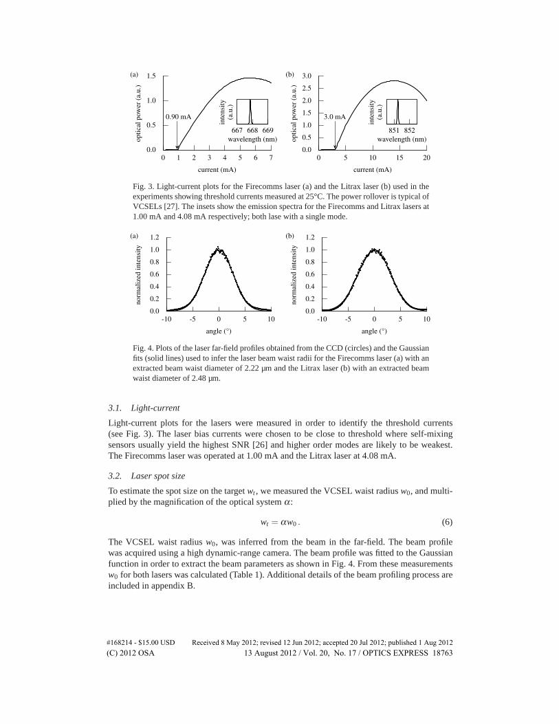
Fig. 4. Plots of the laser far-field profiles obtained from the CCD (circles) and the Gaussianfits (solid lines) used to infer the laser beam waist radii for the Firecomms laser (a) with anextracted beam waist diameter of 2.22 µm and the Litrax laser (b) with an extracted beamwaist diameter of 2.48 µm.

3.1. Light-current

Light-current plots for the lasers were measured in order to identify the threshold currents(see Fig. 3). The laser bias currents were chosen to be close to threshold where self-mixingsensors usually yield the highest SNR [26] and higher order modes are likely to be weakest.The Firecomms laser was operated at 1.00 mA and the Litrax laser at 4.08 mA.

3.2. Laser spot size

To estimate the spot size on the target wt , we measured the VCSEL waist radius w0, and multi-plied by the magnification of the optical system α:

wt = αw0 . (6)

The VCSEL waist radius w0, was inferred from the beam in the far-field. The beam profilewas acquired using a high dynamic-range camera. The beam profile was fitted to the Gaussianfunction in order to extract the beam parameters as shown in Fig. 4. From these measurementsw0 for both lasers was calculated (Table 1). Additional details of the beam profiling process areincluded in appendix B.


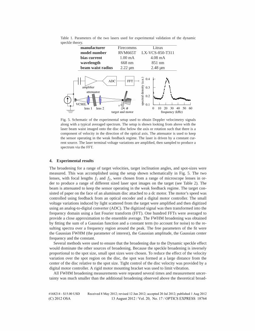
Table 1. Parameters of the two lasers used for experimental validation of the dynamicspeckle theory.

manufacturer Firecomms Litraxmodel number RVM665T LX-VCS-850-T311bias current 1.00 mA 4.08 mAwavelength 668 nm 851 nmbeam waist radius 2.22 µm 2.48 µm

amplifier

ADC FFT

VCSEL

lens 1 lens 2

attenuator

target and motorθ

v 0.1

0.2

0.3

0.4

0 10 20 30 40 50 60

spec

tral

den

sity

(a.u

.)

frequency (kHz)

Fig. 5. Schematic of the experimental setup used to obtain Doppler velocimetry signalsalong with a typical averaged spectrum. The setup is shown looking from above with thelaser beam waist imaged onto the disc disc below the axis or rotation such that there is acomponent of velocity in the direction of the optical axis. The attenuator is used to keepthe sensor operating in the weak feedback regime. The laser is driven by a constant cur-rent source. The laser terminal voltage variations are amplified, then sampled to produce aspectrum via the FFT.

4. Experimental results

The broadening for a range of target velocities, target inclination angles, and spot-sizes weremeasured. This was accomplished using the setup shown schematically in Fig. 5. The twolenses, with focal lengths f1 and f2, were chosen from a range of microscope lenses in or-der to produce a range of different sized laser spot images on the target (see Table 2). Thebeam is attenuated to keep the sensor operating in the weak feedback regime. The target con-sisted of paper on the face of an aluminum disc attached to a dc motor. The motor’s speed wascontrolled using feedback from an optical encoder and a digital motor controller. The smallvoltage variations induced by light scattered from the target were amplified and then digitizedusing an analog-to-digital converter (ADC). The digitized signal was then transformed into thefrequency domain using a fast Fourier transform (FFT). One hundred FFTs were averaged toprovide a close approximation to the ensemble average. The FWHM broadening was obtainedby fitting the sum of a Gaussian function and a constant term (to account for noise) to the re-sulting spectra over a frequency region around the peak. The free parameters of the fit werethe Gaussian FWHM (the parameter of interest), the Gaussian amplitude, the Gaussian centerfrequency and the constant.

Several methods were used to ensure that the broadening due to the Dynamic speckle effectwould dominate the other sources of broadening. Because the speckle broadening is inverselyproportional to the spot size, small spot sizes were chosen. To reduce the effect of the velocityvariation over the spot region on the disc, the spot was formed at a large distance from thecenter of the disc relative to the spot size. Tight control of the disc velocity was provided by adigital motor controller. A rigid motor mounting bracket was used to limit vibration.

All FWHM broadening measurements were repeated several times and measurement uncer-tainty was much smaller than the additional broadening observed above the theoretical broad-


Table 2. The focal lengths and resulting magnifications for lens combinations used to obtaina range of spot sizes on the target.

f1 (mm) f2 (mm) magnification16 26.7 1.678 16 2.0016 40 2.508 26.7 3.338 40 5.00

0

5

10

15

20

25

0 50 100 150 200 250

FW

HM

bro

aden

ing

(kH

z)

target speed (mm/s)

(a)

0

2

4

6

0 50 100 150 200 250

add

itio

nal

bro

aden

ing

(kH

z)

target speed (mm/s)

(c)

0

5

10

15

20

0 50 100 150 200 250 300

FW

HM

bro

aden

ing

(kH

z)

1/w0 (/mm)

(b)

0

2

4

6

0 50 100 150 200 250 300

add

itio

nal

bro

aden

ing

(kH

z)

1/w0 (/mm)

(d)

Fig. 6. Doppler peak broadening for a range of target speeds measured using a 2.5× imag-ing lens configuration (a), and for a range of spot sizes on the target with at a fixed tar-get velocity of 111 mm/s (b). The circles and triangles show the experimental broadeningmeasurements acquired from the Firecomms and Litrax lasers respectively. The solid andbroken lines indicate the theoretical broadening for the Firecomms and Litrax lasers re-spectively. Plots (c) and (d) show the differences between the experimental broadening(which includes all broadening effects) and the theoretical values that only include specklebroadening.

ening due to speckle.

4.1. Effect of target speed on broadening

According to Eq. (4), the broadening is proportional to the target velocity. The target velocitywas varied by changing the disc rotational speed using the motor controller. The target velocitywas calculated from the radial distance measured from the center of the disc to the spot location.The inclination angle was fixed at 10°. Figure 6(a) shows the experimental results and thetheoretical broadening based on the beam waist radii in Table 1 and the 2.5× magnificationfactor of the imaging system.

The experimental broadening is consistently greater than the theoretical speckle broadeningas can be expected due to a range of other factors that contribute to the broadening of theDoppler signal. However, the proportionality of the broadening to the target speed agrees withthe theory. The additional broadening of the measured values is also proportional to the discspeed as can be seen in Fig. 6(c).


0

20

40

60

80

100

120

-20 -10 0 10 20

pea

kfr

equ

ency

(kH

z)

angle (°)

(a)

0

2

4

6

8

10

12

-20 -10 0 10 20

bro

aden

ing

(kH

z)

angle (°)

(b)

Fig. 7. Doppler peak frequency (a) and FWHM broadening (b) with a fixed target speed of111 mm/s over a range of target angles. The circles and triangles show the experimentalbroadening measurements acquired from the Firecomms and Litrax lasers respectively. Thesolid and broken lines indicate the theoretical broadening for the Firecomms and Litraxlaser’s respectively.

4.2. Effect of spot size on broadening

A range of spot sizes were generated using combinations of microscope lenses. The laser spotwas magnified according to the values listed in Table 2. Figure 6(b) show the measured resultsalong with the theoretical broadening. Again, the experimental broadening is consistently largerthan the theoretical broadening. However, in contrast to the additional broadening in Fig. 6(c),the additional broadening in Fig. 6(d) is not strongly correlated to the inverse of the spot size.The slope of the experimental results show a good match to the theory. These results alsoconfirm the independence of broadening on laser wavelength as expected by the theory — thetwo lasers have substantially different wavelengths yet the broadening only depends on the spotsize.

The results in Fig. 6(a) and (b) show two slices through a two-dimensional continuum ofpossible results depending on the spot size and target speed. Based on the results obtained, theadditional spectral broadening over this continuum scales with the target speed, but is relativelyindependent of the laser spot size. The additional broadening may therefore be predominantlydue to an effect that scales with the target speed such as target vibration.

4.3. Effect of target angle on broadening

One perhaps unexpected result from the theoretical investigation was the cosine dependenceof the Doppler signal broadening with target inclination angle. This is in contrast to the peakfrequency fD, in Eq. (5) which has a sine dependence on the target inclination angle.

Figure 7(a) shows the experimentally obtained Doppler peak frequency and the theoreticalvalues in close agreement. Figure 7(b) shows the Doppler broadening results that are largely in-dependent of the target angle. Again, the experimentally obtained broadening results are greaterthan the theory predicts.

5. Conclusions

The speckle theory derived in this paper gives a simple analytic model that can be used topredict spectral broadening for self-mixing sensors. The model provides insight in the depen-dence of Doppler spectrum characteristics as a function of spot size on the target and the targetvelocity. It also shows the interesting independence of the Doppler signal broadening on theangle of incidence for target inclination angles close to normal. This is in contrast to the strongdependence of the Doppler peak frequency on angle. Comparison between the model and theexperimental results was presented for two typical mass-produced VCSELs. The measured


broadening was consistently larger than the theory predicts due to other effects that contributeto broadening. Other contributing effects include the range of velocities present over the illu-minated region on a rotating target, vibration, surface profile variation and the laser linewidth.The experimental results suggest that vibration is the dominant source of the additional broad-ening. However, these contributing mechanisms leading to additional broadening are not offundamental nature, and could be removed by the experimental design.

6. Appendix A: Derivation of the field amplitude autocorrelation function and powerspectrum

In this section we derive the autocorrelation function for the dynamic speckle process for ageneral field distribution. We then solve for the specific case of a Gaussian field and apply asimplification valid for small waist radii to obtain the simple analytic result used in the preced-ing sections of the paper.

The dynamic speckle process is ergodic allowing the time autocorrelation and statistical au-tocorrelation functions to be interchanged [28] or [29]. Both forms are used here as convenient.

Referring to the geometry in Fig. 1, the statistical autocorrelation function of the field ampli-tude RA, at P as a function of times t1 and t2 is [28]

RA(t1, t2) = E [A(t1)A∗(t2)] , (7)

where E[ · ] denotes the expected value operator [30] and A(t) is the complex field amplitude atP.

Because A(t) is a stationary process (a necessary condition for ergodicity), the time differ-ence τ = t2 − t1, only need to be considered. Therefore Eq. (7) can be rewritten as

RA(τ) = E [A(t − τ)A∗(t)] . (8)

If the surface is rough compared to the wavelength, the field at each point, (x,y), reflectedfrom the rough surface of the target is given a phase shift φ , that is uniformly distributed over(−π,π]. We define Ψ(x,y) = eiΦ(x,y) where Φ(x,y) is a random variable for phase shift due tothe rough surface. If the target is inclined at an angle θ , from the perpendicular orientation, thecomplex field reflected from the target will undergo an additional phase shift,

V (x,y) = exp

(i4πx tanθ

λ

). (9)

The complex field reflected and just to the right of the target α(x,y), is given by the productof the incident field U(x,y), the phase shift due to the inclination of the target, and the randomphase shift:

α(x,y) =U(x,y)V (x,y)Ψ(x,y) , (10)

with Ψ(x,y) being a random variable.The Huygens-Fresnel principle can be used to relate the field at the target plane α(x,y),

to the field at the observation point A(ξ ,η). This is approximated by the Fresnel diffractionintegral [22],

A(ξ ,η) =exp

(i 2πz

λ)

iλ zexp

[iπλ z

(ξ 2 +η2)

]

×∫∫ ∞

−∞α(x,y)exp

[iπλ z

(x2 + y2)

]exp

[iπλ z

(ξx+ηy)

]dxdy . (11)


The integral is simplified because only a single point is considered in the observation planeand constant phase terms can be removed without affecting the statistical properties of the phasebecause it is uniformly distributed over (−π,π]. Therefore

A(t) =1

λ z

∫∫ ∞

−∞α(x,y, t)exp

[iπλ z

(x2 + y2)

]dxdy . (12)

We now consider the target in Fig. 1 moving with velocity v. For a fixed laser, the illuminationfield amplitude U(x,y), and the reflected field amplitude are identical and do not change withtime. On the other hand, the random phase variations due to the rough surface Ψ, will be shiftedin the x direction a distance vt cosθ . Therefore, the reflected field just to the right of the roughtarget in Fig. 1 is

α(x,y, t) = Ψ(x+ vt cosθ ,y)U(x,y)V (x,y) . (13)

It is now possible to calculate the autocorrelation function of the field at P, RA(t1, t2), fromEq. (7) using the simplified Fresnel diffraction integral in Eq. (12) and the reflected field givenin Eq. (13).

RA(t1, t2) = E

[1

λ z

∫∫ ∞

−∞Ψ(x+ vt1 cosθ ,y)U(x,y)V (x,y)exp

[iπ

(x2 + y2

)

λ z

]

dxdy

× conj

{1

λ z

∫∫ ∞

−∞Ψ(x+ vt2 cosθ ,y)U(x,y)V (x,y)exp

[iπ

(x2 + y2

)

λ z

]

dxdy

}]

(14)

Where x has been substituted with x + vt cosθ to represent motion in the x direction. It ispossible to consider motion in any direction by altering the orientation of the axes so that thex-axis lies in the direction of motion. Therefore, only considering motion in the x direction doesnot limit the generality of the result.

If the order of integration is changed, the following form is obtained

RA(t1, t2) =1

λ 2z2

∫∫∫∫ ∞

−∞E [Ψ(x1 + vt1 cosθ ,y1)Ψ∗(x2 + vt2 cosθ ,y2)]

×U(x1,y1)V (x1,y1)U∗(x2,y2)V

∗(x2,y2)exp

[iπ

(x2

1 + y21 − x2

2 − y22

)

λ z

]

dx1 dy1 dx2 dy2 . (15)

While Eq. (15) looks complicated, it is dramatically simplified under the assumption of veryfine microstructure of the scattering surface. The spatial autocorrelation of the random phasescreen becomes a delta function [18],

E [Ψ(x1 + vt1 cosθ ,y1)Ψ∗(x2 + vt2 cosθ ,y2)] = δ (x2+vt2 cosθ −x1−vt1 cosθ ,y2−y1) , (16)

which is non-zero only when its parameters are zero. Replacing t2−t1 with τ , Eq. (16) becomes

δ (x2 − x1 + vτ cosθ ,y2 − y1) . (17)

Upon substituting this into Eq. (15), and considering the integration with respect to dx1 and dy1,the delta-function is non-zero when x1 = x2+vτ cosθ and y1 = y2, therefore we can rewrite Eq.(15) as

RA(τ) =1

λ 2z2

∫∫ ∞

−∞U(x2 + vτ cosθ ,y2)V (x2 + vτ cosθ ,y1)U

∗(x2,y2)V∗(x2,y2)

exp

⎧⎨

⎩

iπ[(x2 + vτ cosθ)2 − x2

2

]

λ z

⎫⎬

⎭dx2 dy2 . (18)


The phase terms due to the inclination of the target can be expanded:

V (x2 + vτ cosθ ,y1)V∗(x2,y2) = exp

[i4π(x2 + vτ cosθ) tanθ

λ

]exp

[−i

4πx2 tanθλ

]

= exp

(i4πvτ cosθ tanθ

λ

)

= exp

(i4πvτ sinθ

λ

). (19)

This term, which is related to the Doppler frequency as described subsequently, is independentof x2 and y2, so can be moved outside of the integral in Eq. (18) yielding

RA(τ) =exp

(i 4πvτ sinθ

λ)

λ 2z2

∫∫ ∞

−∞U(x2 + vτ cosθ ,y2)U

∗(x2,y2)

exp

⎧⎨

⎩

iπ[(x2 + vτ cosθ)2 − x2

2

]

λ z

⎫⎬

⎭dx2 dy2 . (20)

This is reproduced in Eq. (1) in Sec. 2 with x2 replaced by x and y2 replaced by y.

6.1. Gaussian field

We now solve the statistical autocorrelation function for the specific case of a Gaussian field.We substitute Eq. (2) into Eq. (1) and solve the integral as follows:

RA(τ) =exp

(i 4πvτ sinθ

λ)

(λ z)2

∫∫ ∞

−∞

4(πw2

t

)2 exp

[

− (x+ vτ cosθ)2 + y2 + x2 + y2

w2t

]

×exp

⎧⎨

⎩

iπ[(x+ vτ cosθ)2 − x2

]

λ z

⎫⎬

⎭dxdy

=4exp

(i 4πvτ sinθ

λ)

(λ zπw2

t

)2

∫ ∞

−∞exp

(−2y2

w2t

)

×∫ ∞

−∞exp

{iπλ z

[(x+ vτ)2 − x2

]− 1

w2t

[(x+ vτ)2 + x2

]}dxdy

=4exp

(i 4πvτ sinθ

λ)

(λ zπw2

t

)2

∫ ∞

−∞exp

(−2y2

w2t

)√πwt√

2exp

[−v2τ2

2

(π2w2

t

λ 2z2 +1

w2t

)]dy

=4

(λ zπw2

t

)2

√πwt

√πwt√

2exp

[−v2τ2

2

(π2w2

t

λ 2z2 +1

w2t

)+ i

4πvτ sinθλ

]

=2√

2

π (λ zwt)2 exp

[−v2τ2

2

(π2w2

t

λ 2z2 +1

w2t

)+ i

4πvτ sinθλ

]. (21)

This result, ignoring the Doppler term, i 4πvτ sinθλ , is in agreement with [9,11] for the case when

the beam waist is located on the target and the distance between the detectors is zero.A(t) will have a Gaussian probability distribution by the central limit theorem because it is

the sum of many independent random variables. Therefore, the autocorrelation function andmean completely describe the random process. Furthermore, the mean m = E[A(t)], is zerobecause E[Ψ(t)] = 0.


VCSEL

screen

camera

lens

CCD array

(c)(a) (b)

Fig. 8. (a) Near-field image of Firecomms laser below threshold (0.21 mA) suggestive ofnon-circular carrier injection. The disc where emission is present is defined by the metal-ization on the front facet of the laser. Non-uniform proton implantation may be responsiblefor the irregular emission shape. (b) Diagram of the setup used to infer the laser near-fieldspot size from a far-field image. (c) A sample far-field image obtained from the CCD array.The speckle caused by the rough surface of the screen is evident in the CCD image.

6.1.1. Simplification for a small Gaussian spot

If wt is small, the π2w2t /λ 2z2 term in Eq. (21) becomes insignificant compared to 1/w2

t , or

π2w4t

λ 2z2 � 1 . (22)

For example, using the experimental conditions for the Litrax laser with the greatest waistradius on the target (12.4 µm), Eq. (22) yields ≈ 0.0002. Making use of this simplification andnormalizing, Eq. (21) becomes:

RA(τ) = exp

(−v2τ2

2w2t+ i

4πvτ sinθλ

). (23)

The normalised spectrum is therefore:

SA( f ) = F{RA(τ)}/max(F{RA(τ)}) = exp

[

−2π2w2t

(f − 2vsinθ

λ)2

v2

]

. (24)

This result is reproduced in Eq. (3) in Sec. 2.2 and plotted in Fig. 2.

7. Appendix B: Experimental procedure used to measure the beam waist radius

For a perfect Gaussian beam it is possible to use a knife-edge technique to measure the focusedspot size directly [31, 32]. However, in this work, the VCSEL near-fields departed from a cir-cular profile. The image of the Firecomms laser near-field taken below threshold in Figure 8(a)is suggestive of non-uniform carrier injection leading to the non-circular near-field profile.

In contrast to the laser near-field profiles, the laser far-field profiles were more circular andprovided good fits to the ideal Gaussian beam profile. Additionally, the relationship betweenthe laser far-field profile and the self-mixing signal power spectrum is more direct. This can beseen by considering that the self-mixing signal power spectrum in Eq. (24) is obtained from theFourier transform of the autocorrelation function in Eq. (1). In the small spot approximation(such that the phase terms in the integral are small), Eq. (1) is simply the autocorrelation of thefield on the target. Recalling the autocorrelation theorem [33],

∫ ∞

−∞f (u) f ∗(u+ x)du = |F{ f}|2 , (25)


the self-mixing signal power spectrum is therefore related to the spatial power spectrum (spatialpower distribution) of the field on the target. In a similar way, and fundamental to the field ofFourier optics [34], the laser far-field intensity (as measured by the CCD array) is also thespatial power spectrum of the laser near-field which is a reduced version of the field on thetarget. Therefore, the laser far-field intensity distribution and the self-mixing power spectrumare closely related.

For these reasons, the laser far-field images were used to infer the laser beam waist radii.Figure 8(b) shows how a CCD array was used to capture an image of the laser far-field profile

that was projected onto a screen [a sample image appears in Fig. 8(c)]. A camera lens was usedto reduce the profile image to fit on the CCD array. The resulting two-dimensional matrix ofintensities from the CCD was reduced to a one-dimensional vector by integrating each verticalcolumn. The vectors obtained for each of the two VCSELs were plotted in Fig. 4. In order toobtain the VCSEL waist radius, the one-dimensional data was fitted to a Gaussian function thatwe now derive. A Gaussian beam [35] has the following intensity profile:

I(x,y) ∝ exp

[−2(x2 + y2)

w2(z)

], (26)

where z is the distance from the beam waist, zR (the Rayleigh parameter) is equal to πw20/λ ,

and

w(z) = w0

√

1+

(zzR

)2

. (27)

The integration of the CCD array columns corresponds to integration over y giving:

I(x) ∝ exp

[− 2x2

w2(z)

]. (28)

In the far-field, z � zR, therefore, w(z) ≈ zλ/(πw0). The laser wavelengths λ , were meas-ured for each laser using an optical spectrum analyzer (Agilent 86140B, resolution 0.07 nm,accuracy ±0.5 nm) for the bias conditions used in the experiments; they are recorded in Table1. Substituting w(z) with the far-field approximation into Eq. (28) and making use of the smallangle approximation, r/z ≈ θ , we obtain:

I(θ) ∝ exp

[

−2

(πθw0

λ

)2]

. (29)

This function was fitted to the data obtained from the CCD images in Fig. 4 in order to extractthe beam-waist radii which appear in Table 1.

Acknowledgements

Russell Kliese is grateful to Thomas Taimre for his valuable feedback while undertaking thework that led to this article. This research was supported under Australian Research CouncilsDiscovery Projects funding scheme (DP0988072).


spectral broadening caused by dynamic speckle in self-mixing

Documents