Supplementary materials for this article are available online. Please click the JASA link at http://pubs.amstat.org.

Spectral Connectivity AnalysisAnn B. LEE and Larry WASSERMAN

Spectral kernel methods are techniques for mapping data into a coordinate system that efficiently reveals the geometric structure—inparticular, the “connectivity”—of the data. These methods depend on tuning parameters. We analyze the dependence of the method onthese tuning parameters. We focus on one particular technique—diffusion maps—but our analysis can be used for other spectral methodsas well. We identify the key population quantities, we define an appropriate risk function for analyzing the estimators, and we explain howthese methods relate to classical kernel smoothing. We also show that, in some cases, fast rates of convergence are possible even in highdimensions. The Appendix of the article is available online as supplementary materials.

KEY WORDS: Diffusion maps; Graph Laplacian; Kernels; Manifold learning; Smoothing; Spectral clustering.

1. INTRODUCTION

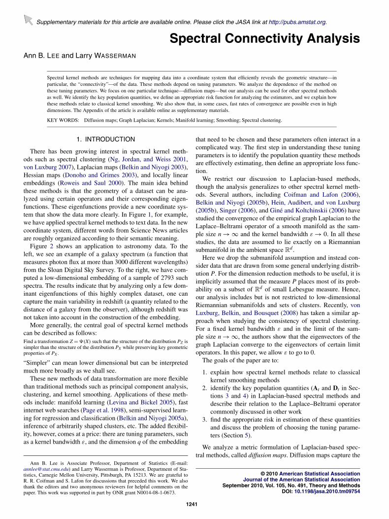
There has been growing interest in spectral kernel meth-ods such as spectral clustering (Ng, Jordan, and Weiss 2001,von Luxburg 2007), Laplacian maps (Belkin and Niyogi 2003),Hessian maps (Donoho and Grimes 2003), and locally linearembeddings (Roweis and Saul 2000). The main idea behindthese methods is that the geometry of a dataset can be ana-lyzed using certain operators and their corresponding eigen-functions. These eigenfunctions provide a new coordinate sys-tem that show the data more clearly. In Figure 1, for example,we have applied spectral kernel methods to text data. In the newcoordinate system, different words from Science News articlesare roughly organized according to their semantic meaning.

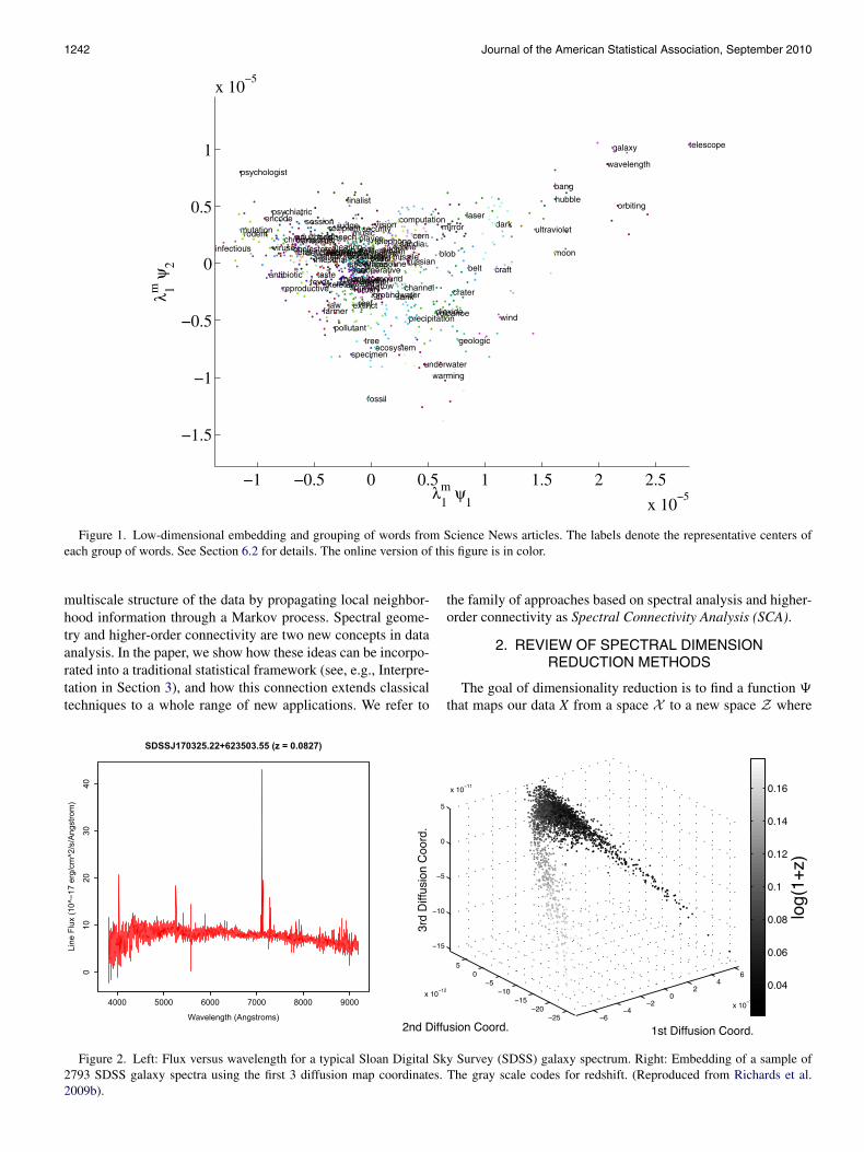
Figure 2 shows an application to astronomy data. To theleft, we see an example of a galaxy spectrum (a function thatmeasures photon flux at more than 3000 different wavelengths)from the Sloan Digital Sky Survey. To the right, we have com-puted a low-dimensional embedding of a sample of 2793 suchspectra. The results indicate that by analyzing only a few dom-inant eigenfunctions of this highly complex dataset, one cancapture the main variability in redshift (a quantity related to thedistance of a galaxy from the observer), although redshift wasnot taken into account in the construction of the embedding.

More generally, the central goal of spectral kernel methodscan be described as follows:Find a transformation Z = �(X) such that the structure of the distribution PZ issimpler than the structure of the distribution PX while preserving key geometricproperties of PX .

“Simpler” can mean lower dimensional but can be interpretedmuch more broadly as we shall see.

These new methods of data transformation are more flexiblethan traditional methods such as principal component analysis,clustering, and kernel smoothing. Applications of these meth-ods include: manifold learning (Levina and Bickel 2005), fastinternet web searches (Page et al. 1998), semi-supervised learn-ing for regression and classification (Belkin and Niyogi 2005a),inference of arbitrarily shaped clusters, etc. The added flexibil-ity, however, comes at a price: there are tuning parameters, suchas a kernel bandwidth ε, and the dimension q of the embedding

Ann B. Lee is Associate Professor, Department of Statistics (E-mail:annlee@stat.cmu.edu) and Larry Wasserman is Professor, Department of Sta-tistics, Carnegie Mellon University, Pittsburgh, PA 15213. We are grateful toR. R. Coifman and S. Lafon for discussions that preceded this work. We alsothank the editors and two anonymous reviewers for helpful comments on thepaper. This work was supported in part by ONR grant N0014-08-1-0673.

that need to be chosen and these parameters often interact in acomplicated way. The first step in understanding these tuningparameters is to identify the population quantity these methodsare effectively estimating, then define an appropriate loss func-tion.

We restrict our discussion to Laplacian-based methods,though the analysis generalizes to other spectral kernel meth-ods. Several authors, including Coifman and Lafon (2006),Belkin and Niyogi (2005b), Hein, Audibert, and von Luxburg(2005b), Singer (2006), and Giné and Koltchinskii (2006) havestudied the convergence of the empirical graph Laplacian to theLaplace–Beltrami operator of a smooth manifold as the sam-ple size n → ∞ and the kernel bandwidth ε → 0. In all thesestudies, the data are assumed to lie exactly on a Riemanniansubmanifold in the ambient space R

d .Here we drop the submanifold assumption and instead con-

sider data that are drawn from some general underlying distrib-ution P. For the dimension reduction methods to be useful, it isimplicitly assumed that the measure P places most of its prob-ability on a subset of R

d of small Lebesgue measure. Hence,our analysis includes but is not restricted to low-dimensionalRiemannian submanifolds and sets of clusters. Recently, vonLuxburg, Belkin, and Bousquet (2008) has taken a similar ap-proach when studying the consistency of spectral clustering.For a fixed kernel bandwidth ε and in the limit of the sam-ple size n → ∞, the authors show that the eigenvectors of thegraph Laplacian converge to the eigenvectors of certain limitoperators. In this paper, we allow ε to go to 0.

The goals of the paper are to:

1. explain how spectral kernel methods relate to classicalkernel smoothing methods

2. identify the key population quantities (At and Dt in Sec-tions 3 and 4) in Laplacian-based spectral methods anddescribe their relation to the Laplace–Beltrami operatorcommonly discussed in other work

3. find the appropriate risk in estimation of these quantitiesand discuss the problem of choosing the tuning parame-ters (Section 5).

We analyze a metric formulation of Laplacian-based spec-tral methods, called diffusion maps. Diffusion maps capture the

© 2010 American Statistical AssociationJournal of the American Statistical Association

September 2010, Vol. 105, No. 491, Theory and MethodsDOI: 10.1198/jasa.2010.tm09754

1241

1242 Journal of the American Statistical Association, September 2010

Figure 1. Low-dimensional embedding and grouping of words from Science News articles. The labels denote the representative centers ofeach group of words. See Section 6.2 for details. The online version of this figure is in color.

multiscale structure of the data by propagating local neighbor-hood information through a Markov process. Spectral geome-try and higher-order connectivity are two new concepts in dataanalysis. In the paper, we show how these ideas can be incorpo-rated into a traditional statistical framework (see, e.g., Interpre-tation in Section 3), and how this connection extends classicaltechniques to a whole range of new applications. We refer to

the family of approaches based on spectral analysis and higher-order connectivity as Spectral Connectivity Analysis (SCA).

2. REVIEW OF SPECTRAL DIMENSIONREDUCTION METHODS

The goal of dimensionality reduction is to find a function �

that maps our data X from a space X to a new space Z where

Figure 2. Left: Flux versus wavelength for a typical Sloan Digital Sky Survey (SDSS) galaxy spectrum. Right: Embedding of a sample of2793 SDSS galaxy spectra using the first 3 diffusion map coordinates. The gray scale codes for redshift. (Reproduced from Richards et al.2009b).

Lee and Wasserman: Spectral Connectivity Analysis 1243

their description is considered to be simpler. Some of the meth-ods naturally lead to an eigen-problem. Below we give someexamples.

2.1 Principal Component Analysis andMultidimensional Scaling

Principal component mapping is a simple and popularmethod for data reduction. In principal component analysis(PCA), one attempts to fit a globally linear model to thedata. If S is a set, define the projection risk R(S) = E‖X −πSX‖2 where πSX is the projection of X onto S. Findingarg minS∈C R(S), where C is the set of all q-dimensional planes,gives a solution that corresponds to the first q eigenvectors ofthe covariance matrix of X.

In “principal coordinate analysis” (PCO), the projectionsπSx = (z1, . . . , zq) on these eigenvectors are used as coordi-nates of the data. This method of data transformation is alsoknown as classical or metric multidimensional scaling (MDS).The goal here is to find a lower-dimensional embedding of thedata that best preserves pairwise Euclidean distances. Assumethat X and Y are covariates in R

p. One way to measure the dis-crepancy between the original configuration and its embeddingis to compute

R(�) = E(d(X,Y)2 − ‖�(X) − �(Y)‖2)

=∫ (

d(x, y)2 − ‖�(x) − �(y)‖2)dP(x)dP(y),

where d(x, y)2 = ‖x−y‖2. One can show that amongst all linearprojections � = πS onto q-dimensional subspaces of R

p, thisquantity is minimized when the data are projected onto theirfirst q principal components (Mardia, Kent, and Bibby 1980).

2.2 Nonlinear Methods

For complex data, a linear approximation may not be ade-quate. There are a large number of nonlinear data reductionmethods; some of these are direct generalizations of the PCAprojection method. For example, local PCA (Kambhatla andLeen 1997) partitions the data space into different regions andfits a hyperplane to the data in each partition. In principal curves(Hastie and Stuetzle 1989), the goal is to minimize a risk of thesame form as the projection risk R(S) but with S representingsome class of smooth curves or surfaces.

Among nonlinear extensions of PCA and MDS, we also havekernel PCA (Schölkopf, Smola, and Müller 1998) which ap-plies PCA to data �(X) in a higher (possibly infinite) dimen-sional “feature space.” The kernel PCA method never explic-itly computes the map �, but instead expresses all calcula-tions in terms of inner products k(x, y) = 〈�(x),�(y)〉 wherethe “kernel” k is a symmetric and positive semi-definite func-tion. Common choices include the Gaussian kernel k(x, y) =exp(−‖x−y‖2

4ε) and the polynomial kernel k(x, y) = 〈x, y〉r ,

where r = 1 corresponds to the linear case in Section 2.1. Asshown in Bengio et al. (2004), the low-dimensional embeddings�(x) used by the eigenmap and spectral clustering methods inSection 2.2.1 are equivalent to the projections [of �(x) on theprincipal axes in feature space] computed by the kernel PCAmethod.

In this paper, we study diffusion maps, a particular spectralembedding technique. Because of the close connection betweenMDS, kernel PCA, and eigenmap techniques, our analysis canbe used for other methods a well. Below we start by provid-ing some background on spectral dimension reduction meth-ods from a more traditional graph-theoretic perspective. In Sec-tion 3 we begin our main analysis.

2.2.1 Laplacian Eigenmaps and Other Locality-PreservingSpectral Methods. The usual strategy in spectral methods isto construct an adjacency graph on a given dataset and thenfind the optimal clustering or encoding of the data that mini-mizes some empirical locality-preserving objective function onthe graph. We define a graph G = (V,E), where the vertexset V = {1, . . . ,n} denotes the observations, and the edge setE represents connections between pairs of observations. Typi-cally, the graph is associated with a weight matrix K that re-flects the “edge masses” or strengths of the edge connections.A common starting point is the Gaussian kernel: Let, for ex-

ample, K(u, v) = exp(−‖xu−xv‖2

4ε) for all data pairs (xu, xv) with

(u, v) ∈ E, and only include cases where the weights K(u, v) areabove some threshold δ in the definition of the edge set E.

Consider now a one-dimensional map f : V → R that as-signs a real value to each vertex; we will later generalizeto the multidimensional case. Many spectral embedding tech-niques are locality preserving; for example, locally linear em-bedding, Laplacian eigenmaps, Hessian eigenmaps, local tan-gent space alignment, etc. These methods are special cases ofkernel PCA, and all aim at minimizing distortions of the formQ(f ) = ∑

v∈V Qv(f ) under the constraints that QM(f ) = 1. Typ-ically, Qv(f ) is a symmetric positive semi-definite quadraticform that measures local variations of f around vertex v, andQM(f ) is a quadratic form that acts as a normalization for f .For Laplacian eigenmaps, for example, the neighborhood struc-ture of G is described in terms of the graph Laplacian matrixL = M − K, where M = diag(ρ1, . . . , ρn) is a diagonal matrixwith ρu = ∑

v K(u, v) for the “node mass” or degree of vertex u.The goal is to find the map f that minimizes the weighted localdistortion

Q(f ) = f TLf =

∑(u,v)∈E

K(u, v)(f (u) − f (v))2 ≥ 0, (1)

under the constraints that QM(f ) = f tMf = ∑

v∈V ρvf (v)2 = 1and (to avoid the trivial solution of a constant function)f T

M1 = 0. Minimizing the distortion in (1) forces f (u) and f (v)to be close if K(u, v) is large. From standard linear algebra itfollows that the optimal embedding is given by the eigenvectorof the generalized eigenvalue problem

Lf = μMf (2)

with the smallest nonzero eigenvalue.We can easily extend the discussion to higher dimensions.

Let f1, . . . , fq be the q first nontrivial eigenvectors of (2), nor-malized so that f T

i Mfj = δij, where δij is Kronecker’s delta func-tion. The map f : V → R

q, where f = (f1, . . . , fq) is the Lapla-cian eigenmap (Belkin and Niyogi 2003) of G in q dimensions.It is optimal in the sense that it provides the q-dimensional em-bedding that minimizes∑

(u,v)∈E

K(u, v)‖f (u) − f (v)‖2 =q∑

i=1

f Ti Lfi (3)

1244 Journal of the American Statistical Association, September 2010

in the subspace orthogonal to M1, under the constraints thatf Ti Mfj = δij for i, j = 1, . . . ,q.

If the data points xu lie on a Riemannian manifold M,and f : M → R is a twice differentiable function, then theexpression in Eq. (1) is the discrete analogue on graphs of∫

M ‖∇Mf ‖2 = − ∫M(Mf )f , where ∇M and M, respec-

tively, are the gradient and Laplace–Beltrami operators on themanifold. The solution of arg min‖f‖=1

∫M ‖∇Mf ‖2 is given by

the eigenvectors of the Laplace–Beltrami operator M. To givea theoretical justification for Laplacian-based spectral methods,several authors have derived results for the convergence of thegraph Laplacian of a point cloud to the Laplace–Beltrami op-erator under the manifold assumption; see Belkin and Niyogi(2005b); Coifman and Lafon (2006); Singer (2006); Giné andKoltchinskii (2006).

2.2.2 Laplacian-Based Methods With an Explicit Metric.Diffusion mapping is an MDS technique that belongs tothe family of Laplacian-based spectral methods. The originalscheme was introduced in the thesis work by Lafon (2004) andin Coifman et al. (2005a, 2005b). See also independent workby Fouss, Pirotte, and Saerens (2005) for a similar techniquecalled Euclidean commute time (ECT) maps. In this paper, wewill describe a slightly modified version of diffusion maps thatappeared in (Coifman and Lafon 2006; Lafon and Lee 2006)(see http://www.stat.cmu.edu/~annlee/software.htm for exam-ple code in Matlab and R).

The starting point of the diffusion framework is to introducea distance metric that reflects the higher-order connectivity ofthe data. This is done by defining a diffusion process or randomwalk on the data. In a graph approach, nodes of the graph rep-resent the observations in the data set. Assuming nonnegativeweights K and a degree matrix M, we define a row-stochasticmatrix A = M

−1K. We then imagine a random walk on the

graph G = (V,E) where A is the transition matrix, and ele-ment A(u, v) corresponds to the probability of reaching node vfrom u in one step. Now if A

m is the mth matrix power of A,then element A

m(u, v) can be interpreted as the probability oftransition from u to v in m steps. By increasing m, we arerunning the Markov chain forward in time, thereby describinglarger scale structures in the data set. Under certain conditionson K, the Markov chain has a unique stationary distributions(v) = ρv/

∑u∈V ρu.

As in multidimensional scaling, the ultimate goal is to find anembedding of the data where Euclidean distances reflect simi-larities between points. In classical MDS, one attempts to pre-serve the original Euclidean distances d2(u, v) = ‖xu − xv‖2 be-tween points. In diffusion maps, the goal is to approximate dif-fusion distances defined by

D2m(u, v) =

∑k∈V

(Am(u, k) − Am(v, k))2

s(k).

This quantity captures the higher-order connectivity of the dataat a scale m and is very robust to noise since it integratesmultiple-step, multiple-path connections between points. Thedistance D2

m(u, v) is small when Am(u, v) is large, or when there

are many paths between nodes u and v in the graph. Further-more, one can show (see Appendix A.1) that the optimal em-bedding in q dimensions is given by the eigenvectors of the

Markov matrix A. In fact, assuming the kernel matrix K is pos-itive semi-definite, we have the “diffusion map”

v ∈ V �→�m(v) = (λm

1 ψ1(v), λm2 ψ2(v), . . . , λ

mq ψq(v)) ∈ R

q,

where {ψ}≥0 are the principal eigenvectors of A and theeigenvalues λ0 = 1 ≥ λ1 ≥ · · · ≥ 0. This solution is, up to arescaling of eigenvectors, the same as the solution of Lapla-cian eigenmaps and spectral clustering, since Lψ = μMψ ifand only if Aψ = λψ for λ = 1 − μ and L = M − K. Thediffusion framework provides a link between Laplacian-basedspectral methods, MDS and kernel PCA. It can be generalizedto multiscale geometries (Coifman and Maggioni 2006), andother locality-preserving methods (Coifman and Lafon 2006).

3. DIFFUSION MAPS

Here we study the diffusion map under the assumption thatthe data are drawn from a general underlying distribution. Byintroducing a Markov chain, the method creates a distribution-sensitive data transformation.

3.1 A Discrete-Time Markov Chain

Definitions. Suppose that the data X1, . . . ,Xn are drawnfrom a distribution P with compact support X ⊂ R

d . We as-sume P has a density p with respect to Lebesgue measure μ.

Let kε(x, y) = 1(4πε)d/2 exp(−‖x−y‖2

4ε) denote the Gaussian ker-

nel (Other kernels can be used. For simplicity, we will focuson the Gaussian kernel which is also the Green’s function ofthe heat equation in R

d .) with bandwidth h = √2ε. We write

the bandwidth in terms of ε instead of h because ε is more nat-ural for our purposes. Consider the Markov chain with transi-tion kernel �ε(x, ·) defined by

�ε(x,A) = P(x → A) =∫

A kε(x, y)dP(y)

pε(x), (4)

where pε(x) = ∫kε(x, y)dP(y).

Starting at x, this chain moves to points y close to x, giv-ing preference to points with high density p(y). In a sense, thischain measures the connectivity of the sample space relativeto p. The stationary distribution Sε is given by

Sε(A) =∫

A pε(x)dP(x)∫pε(x)dP(x)

and Sε(A) →∫

A p(x)dP(x)∫p(x)dP(x)

as ε → 0.

Define the densities ωε(x, y) = d�ε

dμ(x, y) = kε(x,y)p(y)

pε(x)and

aε(x, y) = d�ε

dP(x, y) = kε(x, y)

pε(x).

The diffusion operator Aε—which maps a function f to a newfunction Aεf —is defined by

Aεf (x) =∫

aε(x, y)f (y)dP(y) =∫

kε(x, y)f (y)dP(y)∫kε(x, y)dP(y)

. (5)

We normalize the eigenfunctions {ψε,0,ψε,1, . . .} of Aε by∫ψ2

ε,(x)sε(x)dP(x) = 1, where sε(x) = pε(x)∫pε(y)dP(y)

is the den-

sity of the stationary distribution with respect to P. The first

Lee and Wasserman: Spectral Connectivity Analysis 1245

eigenfunction of the operator Aε is ψε,0(x) = 1 with eigenvalueλε,0 = 1. In general, the eigenfunctions have the following in-terpretation: ψε,j is the smoothest function relative to p, sub-ject to being orthogonal to ψε,i, i < j. The eigenfunctions forman efficient basis for expressing smoothness, relative to p. If adistribution has a few well-defined clusters then the first feweigenfunctions tend to behave like indicator functions (or com-binations of indicator functions) for those clusters. The rest ofthe eigenfunctions provide smooth basis functions within eachcluster. These smooth functions are Fourier-like. Indeed, theuniform distribution on the circle yields the usual Fourier basis.Figure 3 shows a density which is a mixture of two Gaussians.Also shown are the eigenvalues and the first 4 eigenfunctionswhich illustrate these features.

Denote the m-step transition measure by �ε,m(x, ·). Let Aε,mbe the corresponding diffusion operator which can be writ-ten as Aε,mf (x) = ∫

aε,m(x, y)f (y)dP(y) where aε,m(x, y) =d�ε,m/dP.

Define the empirical operator Aε by

Aεf (x) =∑n

i=1 kε(x,Xi)f (Xi)∑ni=1 kε(x,Xi)

=∫

aε(x, y)f (y)dPn(y), (6)

where Pn denotes the empirical distribution, aε(x, y) = kε(x, y)/pε(x) and

pε(x) =∫

kε(x, y)dPn(y) = 1

n

n∑i=1

kε(x,Xi) (7)

is the kernel density estimator. Let Aε,m be the correspondingm-step operator. Let ψε, denote the eigenvectors of the matrixAε where Aε(j, k) = kε(Xj,Xk)/pε(Xj). These eigenvectors areestimates of ψ at the observed values X1, . . . ,Xn. The functionψ(x) can be estimated at values of x not corresponding to one

Figure 3. A mixture of two Gaussians. Density, eigenvalues, andfirst four eigenfunctions. The online version of this figure is in color.

of the Xi’s by kernel smoothing as follows. The eigenfunction-eigenvalue equation λε,ψε, = Aεψε, can be rearranged as

ψε,(x) = Aεψε,

λε,

=∫

kε(x, y)ψε,(y)dP(y)

λε,

∫kε(x, y)dP(y)

(8)

suggesting the estimate

ψε,(x) =∑

i kε(x,Xi)ψε,(Xi)

λε,

∑i kε(x,Xi)

(9)

which is known in the applied mathematics literature as theNyström approximation.

Interpretation. The diffusion operators are averaging oper-ators. Equation (5) arises in nonparametric regression. If we aregiven regression data Yi = f (Xi) + εi, i = 1, . . . ,n, then the ker-nel regression estimator of f is

f (x) = (1/n)∑n

i=1 Yikε(x,Xi)

(1/n)∑n

i=1 kε(x,Xi). (10)

Replacing the sample averages in (10) with their population av-erages yields (5). One may then wonder: in what way is spectralsmoothing different from traditional nonparametric smoothing?There are at least three differences:

1. Estimating Aε is an unsupervised problem, that is, thereare no responses Yi.

2. In spectral smoothing, we are interested in Aε,m for m ≥ 1.The value m = 1 leads to a local analysis of the nearest-neighbor structure—this part is equivalent to classicalsmoothing. Powers m > 1, however, take higher-orderstructure into account. See Section 3.3 for the differencebetween smoothing by diffusion and smoothing by ε.

3. In spectral methods, smoothing is often not the end goal.The eigenvalues and eigenvectors of Aε provide informa-tion on the intrinsic geometry of the data and can be usedto define a new coordinate system for the data.

The concept of connectivity is new in nonparametric sta-tistics and is perhaps best explained in terms of stochasticprocesses. Introduce the forward Markov operator Mεg(x) =∫

X aε(y, x)g(y)dP(y) and its m-step version Mε,m. The firsteigenfunction of Mε is ϕε,0(x) = sε(x), the density of the sta-tionary distribution. In general, ϕε, = sε(x)ψε,(x). The av-eraging operator Aε and the Markov operator Mε and (andhence also the iterates Aε,m and Mε,m) are adjoint under theinner product 〈f ,g〉 = ∫

X f (x)g(x)dP(x), that is, 〈Aεf ,g〉 =〈f ,Mεg〉. By comparing the Gaussian kernel and the heat ker-nel of a continuous-time diffusion process [see equation (3.28)in Grigor’yan 2006], we identify the time step of the discretesystem as t = mε for small ε.

The Markov operator Mε = A∗ε maps measures into mea-

sures. That is, let L1P(X ) = {g : g(y) ≥ 0,

∫g(y)dP(y) = 1}.

Then g ∈ L1P(X ) implies that Mε,mg ∈ L1

P(X ). In particular, if ϕ

is the probability density at time t = 0, then Mε,mϕ is the proba-bility density after m steps. The averaging operator Aε maps ob-servables into observables. Its action is to compute conditionalexpectations. If f ∈ L∞

P (X ) is the test function (observable) att = 0, then Aε,mf ∈ L∞

P (X ) is the average of the function after msteps, that is, at a time comparable to t = mε for a continuoustime system.

1246 Journal of the American Statistical Association, September 2010

3.2 Continuous Time

Under appropriate regularity conditions, the eigenfunctions{ψε,} converge to a set of functions {ψ} as ε → 0. These limit-ing eigenfunctions correspond to some operator. In this sectionwe identify this operator. The key is to consider the Markovchain with infinitesimal transitions. In physics, local infinitesi-mal transitions of a system lead to global macroscopic descrip-tions by integration. Here we use the same tools (infinitesimaloperators, generators, exponential maps, etc.) to extend short-time transitions to larger times.

Define the operator

Gεf (x) = 1

ε

(∫X

aε(x, y)f (y)dP(y) − f (x)

). (11)

Assume that the limit

Gf = limε→0

Gεf = limε→0

Aεf − f

ε(12)

exists for all functions f in some appropriately defined spaceof functions F . The operator G is known as the infinitesimalgenerator. A Taylor expansion shows that

G = − + ∇p

p(13)

for smooth functions where is the Laplacian and ∇ is thegradient. Indeed, Gεf = −f + ∇p

p + O(ε) which is preciselythe bias for kernel regression.

Remark 1. In kernel regression smoothing, the term ∇p/pis considered an undesirable extra bias, called design bias(Fan 1993). In regression it is removed by using local linearsmoothing which is asymptotically equivalent to replacing theGaussian kernel kε with a bias-reducing kernel k∗

ε . In this case,G = −�.

For > 0 define ν2ε, = 1−λε,

εand ν2

= limε→0 ν2ε,. The

eigenvalues and eigenvectors of Gε are −ν2ε, and ψε, while

the eigenvalues and eigenvectors of the generator G are −ν2

and ψ.Let At = limε→0 Aε,t/ε . From (11) and (12), it follows that

At ≡ limε→0

Aε,t/ε = limε→0

(I + εGε)t/ε

= limε→0

(I + εG)t/ε = eGt. (14)

The family {At}t≥0 defines a continuous semigroup of opera-tors (Lasota and Mackey 1994). The notation is summarized inTable 1.

Table 1. Summary of notation

Operator Eigenfunctions Eigenvalues

Aεf (·) =∫

kε(·,y)f (y)dP(y)∫kε(·,y)dP(y)

ψε, λε,

G = limε→0

Aε − I

εψ −ν2

= lim

ε→0

λε, − 1

ε

At = etG =∞∑

=0

e−ν2 t� ψ e−tν2

= limε→0

λt/εε,

= limε→0

Aε,t/ε

One of our goals is to find the bandwidth ε so that Aε,t/ε is agood estimate of At. We show that this is a well-defined prob-lem. Related work on manifold learning, on the other hand, onlydiscusses the convergence properties of the graph Laplacian tothe Laplace–Beltrami operator, that is, the generators of the dif-fusion. Estimating the generator G, however, does not answerquestions regarding the the number of eigenvectors, the numberof groups in spectral clustering, etc.

We can express the diffusion in terms of its eigenfunc-tions. Mercer’s theorem gives the biorthogonal decompositionaε(x, y) = ∑

≥0 λε,ψε,(x)ϕε,(y) and

aε,t/ε(x, y) =∑≥0

λt/εε,ψε,(x)ϕε,(y), (15)

where ψε, are the eigenvectors of Aε , and ϕε, are the eigen-vectors of its adjoint Mε . The details are given in Appendix A.1.Note that {ψ} is an orthonormal basis with respect to the innerproduct 〈f ,g〉ε , while {ϕ} is an orthonormal basis with respectto 〈f ,g〉1/ε = ∫

f (x)g(x)/sε(x)dP(x).From (11), it follows that the eigenvalues λε, = 1 − εν2

ε,.The averaging operator Aε and its generator Gε have the sameeigenvectors. Inserting (15) into (5) and recalling that ϕε,(x) =sε(x)ψε,(x), gives

Aεf (x) =∑≥0

λε,ψε,(x)∫

Xϕε,(y)f (y)dP(y)

=∑≥0

λε,ψε,(x)〈ψε,, f 〉ε =∑≥0

λε,�ε,f (x),

where 〈f ,g〉ε ≡ ∫X f (y)g(y)sε(y)dP(y) and �ε, is the weight-

ed orthogonal projector on the eigenspace spanned by ψε,.Thus, Aε,t/ε = ∑

≥0 λt/εε,�ε,. Similarly, assuming the limit

in (14) exists, At = ∑≥0 e−ν2

t� where � is the weightedorthogonal projector on the eigenspace corresponding to theeigenfunction ψ of G. Weyl’s theorem (Stewart 1991) gives

sup

∣∣e−ν2 t − λ

t/εε,

∣∣ ≤ ∥∥Aε,t/ε − eGt∥∥ = tε + O(ε2),

limε→0

λt/εε, = e−ν2

t, limε→0

�ε, = �. (16)

To estimate the action of the limiting operator At at a giventime t > 0, we need the dominant eigenvalues and eigenvectorsof the generator G. Finally, we also define the limiting tran-sition density at(x, y) = limε→0 aε,t/ε(x, y). As t → 0, at(x, y)converges to a point mass at x; as t → ∞, at(x, y) converges tos(y).

Remark 2. There is an important difference between estimat-ing At and G: the diffusion operator At is a compact operator,while the generator G is not even a bounded operator.

We will consider some examples in Section 6 but let us firstillustrate the definitions for a one-dimensional distribution withmultiscale structure.

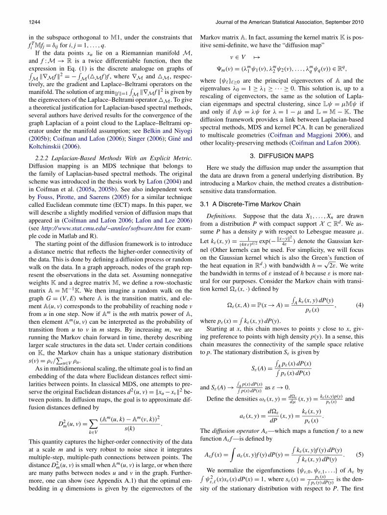
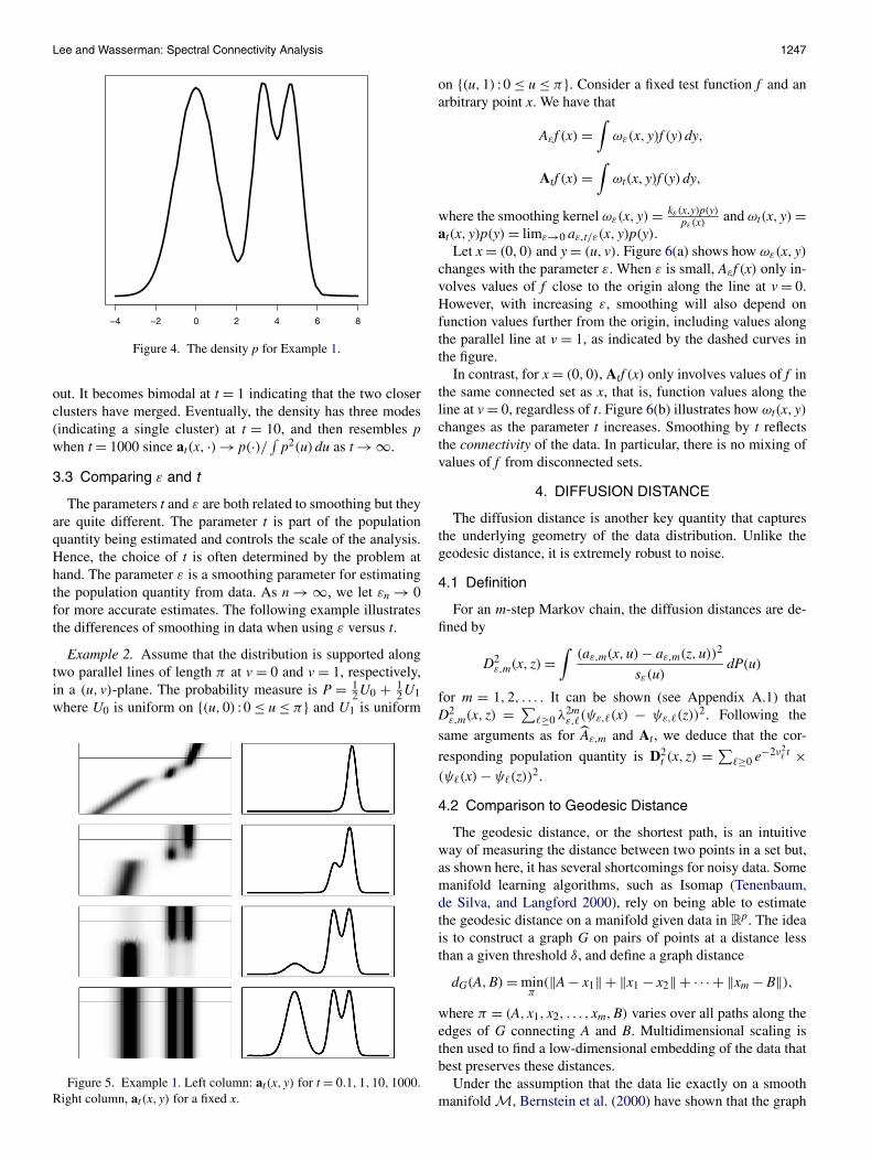
Example 1. Suppose that P is a mixture of three Gaussians.Figure 4 shows the density p. The left column of Figure 5shows At for increasing t. The right column shows at(x, ·) fora fixed x indicated by the horizontal line. The density at(x, ·)starts out concentrated near x. As t increases, it begins to spread

Lee and Wasserman: Spectral Connectivity Analysis 1247

Figure 4. The density p for Example 1.

out. It becomes bimodal at t = 1 indicating that the two closerclusters have merged. Eventually, the density has three modes(indicating a single cluster) at t = 10, and then resembles pwhen t = 1000 since at(x, ·) → p(·)/ ∫

p2(u)du as t → ∞.

3.3 Comparing ε and t

The parameters t and ε are both related to smoothing but theyare quite different. The parameter t is part of the populationquantity being estimated and controls the scale of the analysis.Hence, the choice of t is often determined by the problem athand. The parameter ε is a smoothing parameter for estimatingthe population quantity from data. As n → ∞, we let εn → 0for more accurate estimates. The following example illustratesthe differences of smoothing in data when using ε versus t.

Example 2. Assume that the distribution is supported alongtwo parallel lines of length π at v = 0 and v = 1, respectively,in a (u, v)-plane. The probability measure is P = 1

2 U0 + 12 U1

where U0 is uniform on {(u,0) : 0 ≤ u ≤ π} and U1 is uniform

Figure 5. Example 1. Left column: at(x, y) for t = 0.1,1,10,1000.Right column, at(x, y) for a fixed x.

on {(u,1) : 0 ≤ u ≤ π}. Consider a fixed test function f and anarbitrary point x. We have that

Aεf (x) =∫

ωε(x, y)f (y)dy,

Atf (x) =∫

ωt(x, y)f (y)dy,

where the smoothing kernel ωε(x, y) = kε(x,y)p(y)pε(x)

and ωt(x, y) =at(x, y)p(y) = limε→0 aε,t/ε(x, y)p(y).

Let x = (0,0) and y = (u, v). Figure 6(a) shows how ωε(x, y)changes with the parameter ε. When ε is small, Aεf (x) only in-volves values of f close to the origin along the line at v = 0.However, with increasing ε, smoothing will also depend onfunction values further from the origin, including values alongthe parallel line at v = 1, as indicated by the dashed curves inthe figure.

In contrast, for x = (0,0), Atf (x) only involves values of f inthe same connected set as x, that is, function values along theline at v = 0, regardless of t. Figure 6(b) illustrates how ωt(x, y)changes as the parameter t increases. Smoothing by t reflectsthe connectivity of the data. In particular, there is no mixing ofvalues of f from disconnected sets.

4. DIFFUSION DISTANCE

The diffusion distance is another key quantity that capturesthe underlying geometry of the data distribution. Unlike thegeodesic distance, it is extremely robust to noise.

4.1 Definition

For an m-step Markov chain, the diffusion distances are de-fined by

D2ε,m(x, z) =

∫(aε,m(x,u) − aε,m(z,u))2

sε(u)dP(u)

for m = 1,2, . . . . It can be shown (see Appendix A.1) thatD2

ε,m(x, z) = ∑≥0 λ2m

ε,(ψε,(x) − ψε,(z))2. Following the

same arguments as for Aε,m and At, we deduce that the cor-

responding population quantity is D2t (x, z) = ∑

≥0 e−2ν2 t ×

(ψ(x) − ψ(z))2.

4.2 Comparison to Geodesic Distance

The geodesic distance, or the shortest path, is an intuitiveway of measuring the distance between two points in a set but,as shown here, it has several shortcomings for noisy data. Somemanifold learning algorithms, such as Isomap (Tenenbaum,de Silva, and Langford 2000), rely on being able to estimatethe geodesic distance on a manifold given data in R

p. The ideais to construct a graph G on pairs of points at a distance lessthan a given threshold δ, and define a graph distance

dG(A,B) = minπ

(‖A − x1‖ + ‖x1 − x2‖ + · · · + ‖xm − B‖),where π = (A, x1, x2, . . . , xm,B) varies over all paths along theedges of G connecting A and B. Multidimensional scaling isthen used to find a low-dimensional embedding of the data thatbest preserves these distances.

Under the assumption that the data lie exactly on a smoothmanifold M, Bernstein et al. (2000) have shown that the graph

1248 Journal of the American Statistical Association, September 2010

(a) (b)

Figure 6. Smoothing for data along two parallel lines v = 0 (solid) and v = 1 (dashed). (a) ωε(x, y) for x = (0,0), y = (u, v) andε = 0.01,0.1,1,10. (b) ωt(x, y) for x = (0,0), y = (u, v) and t = 0.01,0.1,1,10.

distance dG(A,B) converges to the geodesic manifold metricdM(A,B) = inf{length(γ )}, where γ varies over the set ofsmooth arcs connecting A and B in M. Beyond this ideal situa-tion, little is known about the statistical properties of the graphdistance. Here we compare the graph distance and the diffu-sion metric for a data set where the support of the distributionis not exactly on a manifold. More specifically, consider a one-dimensional spiral in a plane:{

x = ta cos(bt)

y = ta sin(bt),

where a = 0.8 and b = 10. The geodesic manifold distancedM(A,B) between two reference points A and B with t = π/2band t = 5π/2b, respectively, is 3.46. The corresponding Euclid-ean distance is 0.60.

Example 3 (Sensitivity to noise). We first generate 1000 in-stances of the spiral without noise (i.e., the data fall exactly on

the spiral) and then 1000 instances of the spiral with exponen-tial noise with mean parameter β = 0.09 added to both x and y.For each realization of the spiral, we construct a graph by con-necting all pairs of points at a distance less than a threshold τ .The associated adjacency matrix has only zeros or ones, corre-sponding to the absence or presence of an edge, respectively.

Figure 7(a) shows histograms of the relative change in thegeodesic graph distance (top) and the diffusion distance (bot-tom) when the data are perturbed. (The value 0 corresponds tono change from the average distance in the noiseless cases.)The sample size n = 800 and the neighborhood size τ = 0.15.For the geodesic distance, we have a bimodal distribution witha large variance. The mode near −0.15 corresponds to caseswhere the shortest path between A and B approximately followsthe branch of the spiral; see Figure 8 (left) for an example. Thesecond mode around −0.75 occurs because some realizations ofthe noise give rise to shortcuts, which can dramatically reducethe length of the shortest path; see Figure 8 (right) for an exam-ple. The diffusion distance, on the other hand, is not sensitive to

(a) (b)

Figure 7. Sensitivity to noise. (a) Distribution of the geodesic, top, and diffusion distances, bottom, for a noisy spiral for n = 800 andτ = 0.15. (b) Results for n = 1600 and τ = 0.15. Each histogram has been shifted and rescaled so as to show the relative change from thenoiseless case. The online version of this figure is in color.

Lee and Wasserman: Spectral Connectivity Analysis 1249

Figure 8. Two realizations of a noisy spiral. The solid line represents the shortest path between two reference points A and B in a graphconstructed on the data.

small random perturbations of the data, because unlike the geo-desic distance, it represents an average quantity. Shortcuts dueto noise have little weight in the computation, as the number ofsuch paths is much smaller than the number of paths followingthe shape of the spiral. This is also what our experiment con-firms: Figure 7(a) (bottom) shows a unimodal distribution withabout half the variance as for the geodesic distance.

Example 4 (Increasing sample size). A larger sample size in-creases the chance of shortcuts in the presence of noise for thegeodesic distance. The diffusion distance, on the other hand, be-comes more robust to noise with increasing sample sizes. Thisis illustrated in Figure 7(b) where n = 1600 but the other para-meters (including the neighborhood size τ ) are the same as inExample 3 and Figure 7(a). Choosing the right tuning parame-ters for a given dataset is in general a hard problem. The lackof robustness of the geodesic distance can lead to inconsistentresults while this is of a lesser problem for the diffusion metric.

5. ESTIMATION

In Section 3, we identified At as the key population quantityin Laplacian-based spectral methods. Now we study the prop-erties of Aε,t/ε as an estimator of At. Let �ε, be the orthogonalprojector onto the subspace spanned by ψε, and let � be theprojector onto the subspace spanned by ψ. Consider the fol-lowing operators:

At(ε,P) ≡ Aε,t/ε =∞∑

=0

λt/εε,�ε,,

At(ε,q,P) =q∑

=0

λt/εε,�ε,, At(ε,q, Pn) =

q∑=0

λt/εε,�ε,,

At =∑≥0

e−ν2 t�,

where ψε, and λε, denote the eigenfunctions and eigenvaluesof Aε , and ψε, and λε, are the eigenfunctions and eigenval-ues of the data-based operator Aε . Two estimators of At arethe truncated estimator At(ε,q, Pn) and the nontruncated esti-mator At(ε, Pn) ≡ et(Aε−I)/ε . In practice, truncation is impor-

tant since it corresponds to choosing a dimension for the trans-formed data.

5.1 Estimating the Diffusion Operator At

Given data with a sample size n, we estimate At using a finitenumber q of eigenfunctions and a kernel bandwidth ε > 0. Wedefine the loss function as

Ln(εn,q, t) = ‖At − At(εn,q, Pn)‖, (17)

where ‖B‖ = supf∈F ‖Bf ‖2/‖f ‖2 and ‖f ‖2 =√∫

X f 2(x)dP(x)

where F is the set of uniformly bounded, three times differ-entiable functions with uniformly bounded derivatives whosegradients vanish at the boundary. By decomposing Ln into abias-like and variance-like term, we derive the following resultfor the estimate based on truncation. Define ρ(t) = ∑∞

=1 e−ν2 t.

Theorem 1. Suppose that P has compact support, and hasbounded density p such that infx p(x) > 0 and supx p(x) < ∞.

Let εn → 0 and nεd/2n / log(1/εn) → ∞. Then

Ln(εn,q, t) = ρ(t)(OP(γn) + O(εn)) + Cn

∞∑q+1

e−ν2 t, (18)

where Cn = O(1) and γn =√

log(1/εn)

nε(d+4)/2n

.

The optimal choice of εn is εn � (log n/n)2/(d+8) in whichcase

Ln(εn,q, t) = ρ(t) · OP

(log n

n

)2/(d+8)

+ Cn

∞∑q+1

e−ν2 t. (19)

We also have the following result which does not use trunca-tion.

Theorem 2. Define At(εn, Pn) = et(Aεn−I)/εn . Then, under thesame assumptions on P as in Theorem 1,

‖At − At(εn, Pn)‖ = (OP(γn) + O(εn)) · ρ(t). (20)

The optimal εn is εn � (log n/n)2/(d+8). With this choice,

‖At − At(εn, Pn)‖ = OP

(log n

n

)2/(d+8)

· ρ(t).

1250 Journal of the American Statistical Association, September 2010

See Appendix A.2 for proofs.Let us now make some remarks on the interpretation of these

results.

1. The terms O(εn) and∑∞

q+1 e−ν2 t correspond to bias. The

term OP(γn) corresponds to the square root of the vari-ance.

2. The rate n−2/(d+8) is slow. Indeed, the variance term1/(nε

(d+4)/2n ) is the usual rate for estimating the second

derivative of a regression function which is a notoriouslydifficult problem. This suggests that estimating At accu-rately is quite difficult.

3. We also have that ‖Gε − G‖ = OP(γn) + O(εn), and the

first term is slower than the rate 1/

√nε

(d+2)/2n in Giné and

Koltchinskii (2006) and Singer (2006) where d, in theircase, is the intrinsic dimension of X . The difference inrates is because they assume a uniform distribution. Theslower rate comes from the term pε(x)− pε(x) which can-not be ignored when p is unknown.

4. If the distribution is supported on a manifold of dimen-sion r < d then ε(d+4)/2 becomes ε(r+4)/2. In betweenfull support and manifold support, one can create distri-butions that are concentrated near manifolds. That is, onefirst draws Xi from a distribution supported on a lower-dimensional manifold, then adds noise to Xi. This corre-sponds to full support again unless one lets the varianceof the noise decrease with n. In that case, the exponent ofε can be between r and d.

5. Combining the above results with the result from Zwaldand Blanchard (2006), we have that

‖ψ − ψεn,‖ = (OP(γn)+ O(εn)) · 1

min0≤j≤(ν2j − ν2

j−1).

6. The function ρ(t) is decreasing in t. Hence for large t,the rate of convergence can be arbitrarily fast, even forlarge d. In particular, for t ≥ ρ−1(n−(d+4)/(2(d+8))) theloss has the parametric rate OP(

√log n/n).

7. An estimate of the diffusion distance is

D2t (x, y) =

q∑=0

λ2t/εε, (ψε,(x) − ψε,(y))

2.

The approximation properties are similar to those of At.8. The parameter q = qn should be chosen as small as pos-

sible for dimension reduction, while keeping the last termin (18) no bigger than the first term so as to minimize theloss function Ln. As illustrated below, the optimal q willdepend on the smoothing parameter t, the decay rate ofthe eigenvalues ν and the sample size n.

Example 5. Suppose that ν = β for some β > 1/2. Then

Ln(εn,q, t) = C1

t1/(2β)OP

(log n

n2/(d+8)

)+ C2e−tq2β

.

The smallest qn such that the last term in (18) does not dominateis

qn �((

1

2βlog t + 2

d + 8log n

)/t

)1/(2β)

and we get

Ln(εn,q, t) = OP

(1

t1/(2β)

log n

n2/(d+8)

).

5.2 Nodal Domains and Low Noise

An eigenfunction ψ partitions the sample space into regionswhere ψ has constant sign. This partition is called the nodaldomain of ψ. In some sense, the nodal domain represents thebasic structural information in the eigenfuction. In many appli-cations, such as spectral clustering, it is sufficient to estimatethe nodal domain rather than ψ. We will show that fast ratesare sometimes available for estimating the nodal domain evenwhen the eigenfunctions are hard to estimate. This explains whyspectral methods can be very successful despite the slow ratesof convergence that we and others have obtained.

Formally, the nodal domain of ψ is N = {C1, . . . ,Ck}where the sets C1, . . . ,Ck partition the sample space and thesign of ψ is constant over each partition element Cj. Thus, es-timating the nodal domain corresponds to estimating H(x) =sign(ψ(x)). (If ψ is an eigenfunction then so is −ψ . We im-plicitly assume that the sign ambiguity of the eigenfunction hasbeen removed.)

Recently, in the literature on classification, there has been asurge of research on the so-called “low noise” case. If the datahave a low probability of being close to the decision bound-ary, then very fast rates of convergence are possible even inhigh dimensions. This theory explains the success of classifi-cation techniques in high-dimensional problems. In this sectionwe show that a similar phenomema applies to spectral smooth-ing when estimating the nodal domain.

Inspired by the definition of low noise in Mammen and Tsy-bakov (1999), Audibert and Tsybakov (2007), and Kohler andKrzyzak (2007), we say that P has noise exponent α if thereexists C > 0 such that

P(|ψ1(X)| ≤ δ

) ≤ Cδα. (21)

We are focusing here on ψ1 although extensions to other eigen-functions are immediate. Generally, as two clusters becomewell separated, ψ1 behaves like a step function and P(0 <

|ψ1(X)| ≤ δ) puts less and less mass near 0 which correspondsto α being large.

Theorem 3. Let H(x) = sign(ψ1(x)) and H(x) =sign(ψ1(x)). Suppose that (21) holds. Set εn = n−2/(4α+d+8).Then,

P(H(X) �= H(X)) ≤ n−2α/(4α+8+d), (22)

where X ∼ P.

See Appendix A.2 for proof. Note that, as α → ∞ the ratetends to the parametric rate n−1/2.

5.3 Choosing a Bandwidth

The theory we have developed gives insight into the behav-ior of the methods. But we are still left with the need for apractical method for choosing the smoothing parameter ε. Themost common approach in the machine learning literature isto choose the smallest ε that makes the resulting graph wellconnected. More specifically, von Luxburg (2007) suggests to

Lee and Wasserman: Spectral Connectivity Analysis 1251

“. . . choose ε [in an ε-neighborhood graph] as the length of thelongest edge in a minimal spanning tree of the fully connectedgraph on the data points.” Other methods for selecting ε in-clude Hein, Audibert, and von Luxburg (2005a), Coifman et al.(2008), and Shi, Belkin, and Yu (2009). Instead of using a sin-gle global parameter ε, one can also vary ε over the dataset; see,for example, Zelnik-Manor and Perona (2004). The propertiesof the above approaches for bandwidth selection are howevernot fully understood.

Given the similarity between SCA and kernel smoothing,one may wonder if one can use methods for density esti-mation to choose ε. This turns out to be a nontrivial prob-lem. In density estimation it is common to use the loss func-tion

∫(p(x) − pε(x))2 dx which is equivalent, up to a constant,

to L(ε) = ∫p2ε(x)dx − 2

∫pε(x)p(x)dx. A common method

to approximate this loss is the cross-validation score L(ε) =∫p2ε(x)dx − 2

n

∑ni=1 pε,i(Xi) where pε,i is the same as pε except

that Xi is omitted. It is well known that L(ε) is a nearly unbi-ased estimate of L(ε). One then chooses εn to minimize L(ε).The optimal ε∗

n from our earlier result, however, is (up to logfactors) O(n−2/(d+8)) while the optimal bandwidth ε0

n for mini-mizing L is O(n−2/(d+4)). Hence, ε∗

n/ε0n � n8/((d+4)(d+8)). This

suggests that density cross-validation is not appropriate for ourpurposes.

Estimating the risk is difficult in most problems that are notprediction problems. As usual in nonparametric inference, theproblem is that estimating bias is harder than the original esti-mation problem. Hence, we take a more modest view of simplytrying to find the smallest ε such that the resulting variabilityis tolerable. In other words, we choose the smallest ε that leadsto stable estimates of the eigenstructure (similar to the approachfor choosing the number of clusters in Lange et al. 2004). Thereare several ways to do this. Here are some examples.

Eigen-Stability. Define ψε,(x) = E(ψε,(x)). Althoughψε, �= ψ, they do have a similar shape. We propose to chooseε by finding the smallest ε for which ψε, can be estimated witha tolerable variance. To this end we define

SNR(ε) =√

‖ψε,‖22

E‖ψε, − ψε,‖22

(23)

which we will refer to as the signal-to-noise ratio. When ε issmall, the denominator will dominate and SNR(ε) ≈ 0. Con-versely, when ε is large, the denominator tends to 0 so thatSNR(ε) gets very large. We want to find ε0 such that

ε0 = inf{ε : SNR(ε) ≥ Kn}for some Kn ≥ 1.

We can estimate SNR as follows. We compute B bootstrapreplications ψ

(1)ε, , . . . , ψ

(B)ε, . We then take

SNR(ε) =√

(‖ψ∗ε,‖2

2 − ξ2)+ξ2

, (24)

where c+ = max{c,0}, ξ2 = 1B

∑Bb=1 ‖ψ(b)

ε, − ψ∗ε,‖2

2, and

ψ∗ε, = B−1 ∑B

b=1 ψ(b)ε, . Note that we subtract ξ2 from the nu-

merator to make the numerator approximately an unbiased es-timator of ‖ψε,‖2. Then we use

ε = min{ε : SNR(ε) ≥ Kn}.

See the longer technical report (Lee and Wasserman 2008) forillustrations of the method. For Kn = Cn2/(d+8), where C isa constant, the optimal ε is O(n−2/(d+8)). To see this, writeψε,(x) = ψ(x) + b(x) + ξ(x) where b(x) denotes the bias andξ(x) = ψε,(x) − ψ(x) − b(x) is the random component. Then

SNR2(ε) = ‖ψ(x)+b(x)‖2

E‖ξ‖2 = O(1)

OP(1/(nε(d+4)/2)). Setting this equal

to K2n yields ε0 = O(n−2/(d+8)).

The same bootstrap idea can be applied to estimating thenodal domain. In this case we define

SNR(ε) =√

(‖H∗ε,‖2

2 − ξ2)+ξ2

, (25)

where ξ2 = 1B

∑Bb=1 ‖H(b)

ε, − H∗ε,‖2

2, and H∗ε, = B−1 ×∑B

b=1 H(b)ε, .

Neighborhood Size Stability. Another intuitive way to con-trol the variability is to ensure that the number of points in-volved in the local averages does not get too small. For a givenε let N = {N1, . . . ,Nn} where Ni = #{Xj :‖Xi − Xj‖ ≤ √

2ε}.One can informally examine the histogram of N for various ε.A rule for selecting ε is ε = min{ε : median{N1, . . . ,Nn} ≥ k}.

6. EXAMPLES

6.1 Mixture of Gaussians

We begin with a simple one-dimensional example to illus-trate the different errors in the estimation of eigenvectors. Let

p(x) = 12φ(x;0,1) + 1

4φ(x;3.3,0.5) + 14φ(x;4.7,0.5),

where φ(x;μ,σ) denotes a Normal density with mean μ andvariance σ 2. Figure 4 shows the density. Figure 9 shows the er-ror ‖ψ1 −ψε,1‖ as a function of ε for a sample of size n = 1500.The results are averaged over approximately (we discard sim-ulations where λ1 = λ0 = 1 for ε = 0.02) 200 independentdraws. A minimal error occurs for a range of different val-ues of ε between 0.02 and 0.06. The variance dominates theerror in the small ε region (ε < 0.02), while the bias domi-nates in the large ε region (ε > 0.06). These results are con-sistent with Figure 10, which shows the estimated mean andvariance of the first eigenvector ψε,1 for a few selected valuesof ε (ε = 0.01,0.02,0.06,1), marked with blue circles in Fig-ure 9. Figure 11 shows similar results for the second eigenvec-tor ψ2. Note that even in cases where the error in the estimatesof the eigenvectors is large, the variance around the cross-overpoints (where the eigenvectors switch signs) can be small. Theresults also agree with the conclusion in Section 5.2 that esti-mating the nodal domain of eigenvectors is a simpler problemthan estimating the eigenvectors themselves.

6.2 Words

The next example is an application of SCA to text data min-ing (reproduced from Lafon and Lee 2006). The example showshow one can capture the semantic association of words with dif-fusion distances, and how one can organize and form represen-tative “meta-words” by eigenanalysis and quantization of thediffusion operator.

1252 Journal of the American Statistical Association, September 2010

Figure 9. The error ‖ψ1 − ψε,1‖ in the estimate of the first eigen-vector as a function of ε. For each ε (red dots), an average is takenover approximately 200 independent simulations with n = 1500 pointsfrom a mixture distribution with two Gaussians. Figure 10 shows theestimated mean and variance of ψε,1 for ε = 0.01,0.02,0.06,1 (cir-cles). The online version of this figure is in color.

The data consist of p = 1161 Science News articles. To en-code the text, we extract n = 1004 words and form a document-word information matrix. The mutual information between doc-ument x and word y is defined as Ix,y = log(

ncx,y∑ξ cξ,y

∑η cx,η

),

where cx,y is the number of times word y appears in documentx. Let ey = [I1,y, I2,y, . . . , Ip,y] be a p-dimensional feature vec-tor for word y.

Our goal is to reduce both the dimension p and the numberof words n, while preserving the main connectivity structure of

Figure 10. The first eigenvector ψε,1 for ε = 0.01,0.02,0.06,1,and n = 1500. The red dashed curves with shaded regions indicate themean value ± two standard deviations for approximately 200 indepen-dent simulations. The black solid curves show ψε,1 as ε → 0.

Figure 11. The second eigenvector ψε,2 for ε = 0.01,0.02,0.06,1,and n = 1500. The red dashed curves with shaded regions indicate themean value ± two standard deviations for approximately 200 indepen-dent simulations. The black solid curves show ψε,2 as ε → 0.

the data. In addition, we seek a coordinate system for the wordsthat reflect how similar they are in meaning. Diffusion mapsand quantization of the diffusion operator (diffusion coarse-graining) by k-means offer a natural framework for achievingthese objectives.

We construct a graph where each node is a word and definethe weight matrix by K(i, j) = exp(−‖ei−ej‖2

4ε). Let Aε,m be the

corresponding m-step transition matrix with eigenvalues λm and

eigenvectors ψ. Using the bootstrap, we estimate the SNR ofψ1 as a function of ε. A SNR cut-off at 2, gives the bandwidthε = 150. For m = 3, q = 12 and this choice of bandwidth, wehave a spectral fall-off (λq/λ1)

m < 0.1, that is, we can obtaina dimensionality reduction of a factor of about 1/100 by theeigenmap ey ∈ R

p �→ (λm1 ψ1(y), λm

2 ψ2(y), . . . , λmq ψq(y)) ∈ R

q

without losing much accuracy. Further, to reduce the size of thedataset, we form a quantized matrix Aε,m for a coarse-grainedrandom walk on a graph with k < n nodes. It can be shown(Lafon and Lee 2006), that the spectral properties of Aε,m andAε,m are similar when the coarse-graining (quantization) corre-sponds to k-means clustering in diffusion space.

Figure 1 shows the first two diffusion coordinates of the clus-ter centers (the “meta-words”) for k = 100. These representa-tive words have roughly been rearranged according to their se-mantics and can be used as conceptual indices for documentrepresentation and text retrieval. Starting to the left, movingcounter clockwise, we here have words that express conceptsin medicine, biology, earth sciences, physics, astronomy, com-puter science, and social sciences. Table 2 gives examples ofwords in a cluster and the corresponding word centers.

7. DISCUSSION

Spectral methods are rapidly gaining popularity. Their abil-ity to reveal nonlinear structure makes them ideal for complex,high-dimensional problems. We have attempted to provide in-sight into these techniques by identifying the key population

Lee and Wasserman: Spectral Connectivity Analysis 1253

Table 2. Examples of word groupings

Word center Remaining words in group

Virus aids, allergy, hiv, vaccine, viralReproductive fruit, male, offspring, reproductive, sex, spermVitamin calory, drinking, fda, sugar, supplement, vegetableFever epidemic, lethal, outbreak, toxinEcosystem ecologist, fish, forest, marine, river, soil, tropicalWarming climate, el, nino, forecast, pacific, rain, weather, winterGeologic beneath, crust, depth, earthquake, plate, seismic, trapped, volcanicLaser atomic, beam, crystal, nanometer, optical, photon, pulse, quantum, semiconductorHubble dust, gravitational, gravity, infraredGalaxy cosmic, universeFinalist award, competition, intel, prize, scholarship, student, talent, winner

quantities (namely the operators At and Dt), and studying thelarge sample properties of their estimates.

Our analysis shows that spectral kernel methods in mostcases have a convergence rate similar to classical nonparamet-ric smoothing. Laplacian-based kernel methods, for example,use the same smoothing operators as in traditional nonparamet-ric regression. The end goal however is not smoothing, but datatransformation and structure definition of data. Spectral meth-ods exploit the fact that the eigenvectors of local smoothingoperators provide a coordinate system and information on theunderlying geometry and connectivity of the data.

We close by giving examples of how SCA can be a pow-erful tool in high-dimensional “geometry-based” data analy-sis. Some of these applications (such as spectral clustering)are well known while others (such as sparse coding and high-dimensional density estimation via SCA) are new. The full de-tails are reported in separate papers.

7.1 Clustering and Sparse Coding

One approach to clustering is spectral clustering (Ng, Jordan,and Weiss 2001; von Luxburg 2007). The idea is to transformthe data using the first few nontrivial eigenvectors ψ1, . . . ,ψm

and then apply a standard clustering algorithm such as k-meansclustering. This approach can be quite effective for finding non-spherical clusters.

On a related note, the output from spectral clustering can beused for encoding of massive datasets. Consider a training set ofsignals X1, . . . ,Xn in R

p. In classical sparse coding (Olshausenand Field 1997), one seeks a dictionary, that is, a set of basisvectors, D and vectors βi to minimize an empirical cost func-tion, typically of the form R(D, {βi}) = ∑n

i=1(‖Xi − Dβi‖2 +λ‖βi‖1), where λ is a regularization parameter. For complexdata, however, the sparsity constraint on the coefficients βi’sand the assumption that Xi ≈ Dβi can be overly restrictive. Non-linear geometries are also not taken into account.

An alternative approach to basis learning is to first transformthe data via SCA, and then further quantize the data structure bya weighted k-means algorithm in the embedding space (Lafonand Lee 2006); see Section 6.2 for an application to words. Thek centroids c1, . . . , cn form “prototypes” of the data. By con-struction, they capture the underlying geometry of the distrib-ution PX and form a more efficient covering of the data space.Richards et al. (2009a) use geometric prototyping to construct a

basis of simple stellar population (SSP) spectra. For simulatedgalaxy spectra, such an approach to basis learning leads to moreaccurate estimation of star formation history than a hand-pickedsubset of SSP’s (Cid Fernandes 2005; Asari et al. 2007) or basesderived from PCA or sparse methods.

7.2 Density Estimation

If Q is a quantization map then the quantized density estima-tor (Meinicke and Ritter 2002) is p(x) = (1/n)

∑ni=1(1/hd) ×

K(‖x−Q(Xi)‖

h ). For highly clustered data, the quantized densityestimator can have smaller mean squared error than the usualkernel density estimator. Similarly, we can define the quantizeddiffusion density estimator as

p(x) = 1

n

n∑i=1

1

hdK

(Dt(x,Xi)

h

)(26)

which can potentially have small mean squared error for appro-priately chosen t.

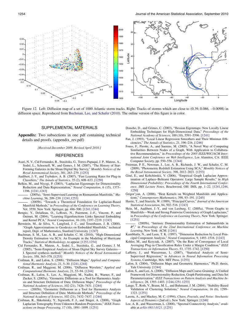
SCA can be a powerful tool for high-dimensional density es-timation problems where standard statistical methods are inad-equate. Buchman, Lee, and Schafer (2010), for example, usethe density estimator in Eq. (26) for modeling and simulationof hurricane tracks. In the analysis, a datum represents an en-tire hurricane trajectory (see Figure 12); densities are estimatedfrom observed tracks in a lower-dimensional diffusion space;a random sample is drawn from the estimated diffusion den-sity; the sample is finally mapped back into the original trackspace to simulate as-yet-unobserved tracks.

7.3 Regression

Incorporating data geometry can also radically improve re-gression and classification (Belkin and Niyogi 2005a; Laffertyand Wasserman 2007; Singh, Nowak, and Zhu 2008). A com-mon method for nonparametric regression is to expand the re-gression function m(x) = E(Y|X = x) in a basis and then es-timate the coefficients of the expansion from the data. Usu-ally, the basis is chosen beforehand. The diffusion map basisprovides a data-adaptive basis for doing nonparametric regres-sion. We expand m(x) = E(Y|X = x) as m(x) = ∑

j βjψj(x).

Let m(x) = ∑qj=1 βjψε,j(x) where q and ε are chosen by cross-

validation. See (Richards et al. 2009b) and Freeman et al.(2009) for applications to redshift prediction of Sloan DigitalSky Survey (SDSS) data, and performance comparisons to PCAand template matching.

1254 Journal of the American Statistical Association, September 2010

Figure 12. Left: Diffusion map of a set of 1000 Atlantic storm tracks. Right: Tracks of storms which are close to (0.39,0.086,−0.0098) indiffusion space. Reproduced from Buchman, Lee, and Schafer (2010). The online version of this figure is in color.

SUPPLEMENTAL MATERIALS

Appendix: Two subsections in one pdf containing technicaldetails and proofs. (appendix_rev.pdf)

[Received December 2009. Revised April 2010.]

REFERENCES

Asari, N. V., Cid Fernandes, R., Stasinska, G., Torres-Papaqui, J. P., Mateus, A.,Sodré, L., Schoenell, W., and Gomes, J. M. (2007), “The History of Star-Forming Galaxies in the Sloan Digital Sky Survey,” Monthly Notices of theRoyal Astronomical Society, 381, 263–279. [1253]

Audibert, J.-Y., and Tsybakov, A. B. (2007), “Fast Learning Rates for Plug-inClassifiers,” The Annals of Statistics, 35 (2), 608–633. [1250]

Belkin, M., and Niyogi, P. (2003), “Laplacian Eigenmaps for DimensionalityReduction and Data Representation,” Neural Computation, 6 (15), 1373–1396. [1241,1243]

(2005a), “Semi-Supervised Learning on Riemannian Manifolds,” Ma-chine Learning, 56, 209–239. [1241,1253]

(2005b), “Towards a Theoretical Foundation for Laplacian-BasedManifold Methods,” in Proceedings of the Conference on Learning Theory,Vol. 3559, New York: Springer, pp. 486–500. [1241,1244]

Bengio, Y., Delalleau, O., LeRoux, N., Paiement, J.-F., Vincent, P., andOuimet, M. (2004), “Learning Eigenfunctions Links Spectral Embeddingand Kernel PCA,” Neural Computation, 16 (10), 2197–2219. [1243]

Bernstein, M., de Silva, V., Langford, J. C., and Tenenbaum, J. B. (2000),“Graph Approximations to Geodesics on Embedded Manifolds,” technicalreport, Dept. of Mathematics, Stanford University. [1247]

Buchman, S. M., Lee, A. B., and Schafer, C. M. (2010), “High-DimensionalDensity Estimation via SCA: An Example in the Modeling of HurricaneTracks,” Statistical Methodology, to appear. [1253,1254]

Cid Fernandes, R., Mateus, A., Sodré, L., Stasinska, G., and Gomes, J. M.(2005), “Semi-Empirical Analysis of Sloan Digital Sky Survey Galaxies—I. Spectral synthesis method,” Monthly Notices of the Royal AstronomicalSociety, 358, 363–378. [1253]

Coifman, R., and Lafon, S. (2006), “Diffusion Maps,” Applied and Computa-tional Harmonic Analysis, 21, 5–30. [1241,1244]

Coifman, R., and Maggioni, M. (2006), “Diffusion Wavelets,” Applied andComputational Harmonic Analysis, 21, 53–94. [1244]

Coifman, R., Lafon, S., Lee, A., Maggioni, M., Nadler, B., Warner, F., andZucker, S. (2005a), “Geometric Diffusions as a Tool for Harmonics Analy-sis and Structure Definition of Data: Diffusion Maps,” Proceedings of theNational Academy of Sciences, 102 (21), 7426–7431. [1244]

(2005b), “Geometric Diffusions as a Tool for Harmonics Analysisand Structure Definition of Data: Multiscale Methods,” Proceedings of theNational Academy of Sciences, 102 (21), 7432–7437. [1244]

Coifman, R., Shkolnisky, Y., Sigworth, F. J., and Singer, A. (2008), “GraphLaplacian Tomography From Unknown Random Projections,” IEEE Trans-actions on Image Processing, 17 (10), 1891–1899. [1251]

Donoho, D., and Grimes, C. (2003), “Hessian Eigenmaps: New Locally LinearEmbedding Techniques for High-Dimensional Data,” Proceedings of theNational Academy of Sciences, 100 (10), 5591–5596. [1241]

Fan, J. (1993), “Local Linear Regression Smoothers and Their Minimax Effi-ciencies,” The Annals of Statistics, 21, 196–216. [1246]

Fouss, F., Pirotte, A., and Saerens, M. (2005), “A Novel Way of ComputingSimilarities Between Nodes of a Graph, With Application to Collabora-tive Recommendation,” in Proceedings of the 2005 IEEE/WIC/ACM Inter-national Joint Conference on Web Intelligence, Los Alamitos, CA: IEEEComputer Society, pp. 550–556. [1244]

Freeman, P. E., Newman, J., Lee, A. B., Richards, J. W., and Schafer, C. M.(2009), “Photometric Redshift Estimation Using SCA,” Monthly Notices ofthe Royal Astronomical Society, 398, 2012–2021. [1253]

Giné, E., and Koltchinskii, V. (2006), “Empirical Graph Laplacian Approx-imation of Laplace–Beltrami Operators: Large Sample Results,” in HighDimensional Probability: Proceedings of the Fourth International Confer-ence. IMS Lecture Notes, Beachwood, OH: IMS, pp. 1–22. [1241,1244,1250]

Grigor’yan, A. (2006), “Heat Kernels on Weighted Manifolds and Applica-tions,” Contemporary Mathematics, 398, 93–191. [1245]

Hastie, T., and Stuetzle, W. (1989), “Principal Curves,” Journal of the AmericanStatistical Association, 84, 502–516. [1243]

Hein, M., Audibert, J.-Y., and von Luxburg, U. (2005a), “From Graphs toManifolds—Weak and Strong Pointwise Consistency of Graph Laplacians,”in Proceedings of the Conference on Learning Theory, New York: Springer.[1251]

(2005b), “Intrinsic Dimensionality Estimation of Submanifolds inRd ,” in Proceedings of the 22nd International Conference on MachineLearning, New York: ACM. [1241]

Kambhatla, N., and Leen, T. K. (1997), “Dimension Reduction by Local Prin-cipal Component Analysis,” Neural Computation, 9, 1493–1516. [1243]

Kohler, M., and Krzyzak, A. (2007), “On the Rate of Convergence of LocalAveraging Plug-in Classification Rules Under a Margin Condition,” IEEETransactions on Information Theory, 53, 1735–1742. [1250]

Lafferty, J., and Wasserman, L. (2007), “Statistical Analysis of Semi-Supervised Regression,” in Advances in Neural Information ProcessingSystems, Cambridge, MA: MIT Press. [1253]

Lafon, S. (2004), “Diffusion Maps and Geometric Harmonics,” Ph.D. thesis,Yale University. [1244]

Lafon, S., and Lee, A. (2006), “Diffusion Maps and Coarse-Graining: A UnifiedFramework for Dimensionality Reduction, Graph Partitioning, and Data SetParameterization,” IEEE Transactions on Pattern Analysis and Machine In-telligence, 28, 1393–1403. [1244,1251-1253]

Lange, T., Roth, V., Braun, M. L., and Buhmann, J. M. (2004), “Stability-BasedValidation of Clustering Solutions,” Neural Computation, 16 (6), 1299–1323. [1251]

Lasota, A., and Mackey, M. C. (1994), Chaos, Fractals, and Noise: StochasticAspects of Dynamics (2nd ed.), New York: Springer. [1246]

Lee, A. B., and Wasserman, L. (2008), “Spectral Connectivity Analysis,” avail-able at arXiv:0811.0121. [1251]

Lee and Wasserman: Spectral Connectivity Analysis 1255

Levina, E., and Bickel, P. J. (2005), “Maximum Likelihood Estimation of In-strinsic Dimension,” in Advances in Neural Information Processing Sys-tems, Vol. 17. [1241]

Mammen, E., and Tsybakov, A. B. (1999), “Smooth Discrimination Analysis,”The Annals of Statistics, 27, 1808–1829. [1250]

Mardia, K. V., Kent, J. T., and Bibby, J. M. (1980), Multivariate Analysis, Aca-demic Press. [1243]

Meinicke, P., and Ritter, H. (2002), “Quantizing Density Estimators,” in Ad-vances in Neural Information Processing Systems, Vol. 14, Cambridge,MA: MIT Press, pp. 825–832. [1253]

Ng, A. Y., Jordan, M. I., and Weiss, Y. (2001), “On Spectral Clustering: Analy-sis and an Algorithm,” in Advances in Neural Information Processing Sys-tems, Cambridge, MA: MIT Press. [1241,1253]

Olshausen, B. A., and Field, D. J. (1997), “Sparse Coding With an Overcom-plete Basis Set: A Strategy Employed by V1?” Vision Research, 37, 3311–3325. [1253]

Page, L., Brin, S., Motwani, R., and Winograd, T. (1998), “The Pagerank Cita-tion Ranking: Bringing Order to the Web,” technical report, Stanford Uni-versity. [1241]

Richards, J. W., Freeman, P. E., Lee, A. B., and Schafer, C. M. (2009a), “Ac-curate Parameter Estimation for Star Formation History in Galaxies UsingSDSS Spectra,” Monthly Notices of the Royal Astronomical Society, 399,1044–1057. [1253]

(2009b), “Exploiting Low-Dimensional Structure in AstronomicalSpectra,” Astrophysical Journal, 691, 32–42. [1242,1253]

Roweis, S., and Saul, L. (2000), “Nonlinear Dimensionality Reduction by An-nalsly Linear Embedding,” Science, 290, 2323–2326. [1241]

Schölkopf, B., Smola, A., and Müller, K.-R. (1998), “Nonlinear ComponentAnalysis as a Kernel Eigenvalue Problem,” Neural Computation, 10 (5),1299–1319. [1243]

Shi, T., Belkin, M., and Yu, B. (2009), “Data Spectroscopy: Eigenspaces ofConvolution Operators and Clustering,” The Annals of Statistics, 37 (6B),3960–3984. [1251]

Singer, A. (2006), “From Graph to Manifold Laplacian: The ConvergenceRate,” Applied and Computational Harmonic Analysis, 21, 128–134. [1241,1244,1250]

Singh, A., Nowak, R., and Zhu, X. (2008), “Unlabeled Data: Now It Helps,Now It Doesn’t,” in Advances in Neural Information Processing Systems,Red Hook, NY: Curran Associates, Inc. [1253]

Stewart, G. (1991), Perturbation Theory for the Singular Value Decomposition,SVD and Signal Processing, Vol. II, New York: Elsevier Science. [1246]

Tenenbaum, J. B., de Silva, V., and Langford, J. C. (2000), “A Global GeometricFramework for Nonlinear Dimensionality Reduction,” Science, 290 (5500),2319–2323. [1247]

von Luxburg, U. (2007), “A Tutorial on Spectral Clustering,” Statistics andComputing, 17 (4), 395–416. [1241,1250,1253]

von Luxburg, U., Belkin, M., and Bousquet, O. (2008), “Consistency of Spec-tral Clustering,” The Annals of Statistics, 36 (2), 555–586. [1241]

Zelnik-Manor, L., and Perona, P. (2004), “Self-Tuning Spectral Clustering,” inAdvances in Neural Information Processing Systems, Vol. 17, Cambridge,MA: MIT Press, pp. 1601–1608. [1251]

Zwald, L., and Blanchard, G. (2006), “On the Convergence of Eigenspaces inKernel Principal Component Analysis,” in Advances in Neural InformationProcessing Systems, Vol. 18, Cambridge, MA: MIT Press, pp. 1649–1656.[1250]