spectral sparse bayesian learning reflectivity inversion...

Geophysical Prospecting doi: 10.1111/1365-2478.12000

Spectral sparse Bayesian learning reflectivity inversion

Sanyi Yuan1,2 and Shangxu Wang1,2∗1State Key Laboratory of Petroleum Resource and Prospecting, China University of Petroleum, Beijing 102249, China, and 2CNPC KeyLaboratory of Geophysical Exploration, China University of Petroleum, Beijing 102249, China

Received February 2011, revision accepted August 2012

ABSTRACTA spectral sparse Bayesian learning reflectivity inversion method, combining spectralreflectivity inversion with sparse Bayesian learning, is presented in this paper. Themethod retrieves a sparse reflectivity series by sequentially adding, deleting or re-estimating hyper-parameters, without pre-setting the number of non-zero reflectivityspikes. The spikes with the largest amplitude are usually the first to be resolved. Themethod is tested on a series of data sets, including synthetic data, physical modellingdata and field data sets. The results show that the method can identify thin beds belowtuning thickness and highlight stratigraphic boundaries. Moreover, the reflectivityseries, which is inverted trace-by-trace, preserves the lateral continuity of layers.

Key words: Reflectivity inversion, Sparse Bayesian learning, Thin bed, Bayesianinversion.

1 INTRODUCT I ON

One of the aims of seismic exploration is to obtain a sub-surface image from reflected seismic data. However, reflectedseismic data are band-limited, which results in limited reso-lution (Widess 1973). Thus, many techniques have been de-veloped to remove the wavelet from the seismic data, for thepurpose of retrieving the reflectivity series and identifying anythin layers.

The most popular method to retrieve reflectivity is inversefiltering within a least-squares framework (e.g., Berkhout1977; Robinson and Treitel 1980; Bickel and Martinez 1983).This method is based on the assumption that the earth’s re-flectivity has a spectrum of white noise, so that the autocorre-lation of the wavelet can be replaced by that of seismic data.Therefore, the influence of the wavelet is removed. However,the fact that the wavelet is band-limited means that the resultsof the reflectivity inversion are non-unique.

In order to overcome or alleviate this ambiguity, it is com-mon to assume that the reflectivity series is sparse. Based onsuch a sparsity constraint, many deconvolution or reflectiv-

∗E-mail: [email protected]

ity inversion methods have been proposed. One such methodis to use a non-linear function, for example, an L1 norm,entropy norm, Cauchy criterion or Huber criterion, as a reg-ularization term to promote a sparse reflectivity estimation(e.g., Levy and Fullagar 1981; Sacchi, Velis and Cominguez1994; Sacchi 1997). Another kind of method is to adopt aBayesian framework, such as maximizing a likelihood func-tion or maximizing a posteriori density function with theassumption that the reflectivity series obeys a certain priordistribution (e.g., Kormylo and Mendel 1983; Chi, Mendeland Hampson 1984; Debeye and van Riel 1990). This canbe utilized to obtain sparse reflectivity. Besides, by pre-settingthe number of non-zero reflectivity spikes, sparse reflectivityinversion methods based on global optimization algorithms,such as simulated annealing, particle swarm optimization orant colony optimization, can also be introduced (e.g., Vester-gaard and Mosegaard 1991; Velis 2008; Yuan, Wang andTian 2009).

Recently, different methods based on matching pursuit(MP), orthogonal matching pursuit (OMP) or basis pursuit(BP) algorithms have been developed to implement sparse re-flectivity inversion. Nguyen and Castagna (2010) presenteda high-resolution seismic reflectivity inversion method basedon a MP algorithm with the incorporation of well-log derived

C© 2013 European Association of Geoscientists & Engineers 1

2 S. Yuan and S. Wang

patterns. Yang et al. (2011) also presented a MP reflectivityinversion method that utilized thin-bed models as a dictionary.For these two methods, a priori information such as the num-ber, thickness and reflection strength of the thin-beds are usedas constraint conditions to obtain a reliable result. Broadheadand Tonellot (2010) presented a sparse deterministic decon-volution method based on an OMP algorithm, a fast MP al-gorithm, by using the time-shift wavelets or the convolutionmatrix of the wavelet. Zhang and Castagna (2011) presenteda seismic sparse-layer reflectivity inversion method based ona BP algorithm, by utilizing wedge-models as a dictionary.

Sparse Bayesian Learning (SBL) has been proposed andproven to be an effective and accurate method for a wide vari-ety of regression and classification problems (Tipping 2001).The SBL paradigm performs parameter learning via type-II maximum likelihood or evidence maximization (Mackay1992) where marginal likelihood maximization leads to auto-matic identification of the relevant kernels and hence sparsifiesthe model. The SBL model is known to enjoy many advan-tages, such as probabilistic prediction, the facility to utilize ar-bitrary basis functions and automatic estimation of nuisanceparameters. This model has been successful in a wide rangeof applications such as visual tracking (Williams, Blake andCipolla 2005), text classification (Silva and Ribeiro 2006),image processing (Demir and Erturk 2007), positron emissiontomography (Peng et al. 2008) and dynamic light scattering(Nyeo and Ansari 2011).

In the context of signal processing, for basis vectors selec-tion or sparse signal representation problems, SBL, similar toOMP, sequentially updates the basis vectors. The main dif-ference between them is that SBL updates hyper-parametercontrolling weights, while OMP directly updates weights. It isimportant to note that in the context of this paper the weightsin the algorithm are the reflectivity of the earth. Comparedwith OMP, the main advantages (Ji, Xue and Carin 2008) forSBL are that 1) it deletes the basis vector that has been chosento maintain a more concise signal representation; 2) it yields‘error bars’ for the estimated weights, indicating the confi-dence. In contrast to the BP algorithm, the main differencesare that 1) BP updates all weights for every iteration, whileSBL mainly updates one weight for every iteration; 2) the re-sult of BP is not exactly sparse due to noisy reconstruction,while that of SBL is strictly sparse without background os-cillation in the model; 3) BP adopts a fixed sparsity-inducingprior to encourage sparsity, while SBL uses a parametrizedprior to automatically control sparsity. In addition, SBL hasthe advantage of preventing any ‘structural errors’ (at least inthe absence of noise) (Wipf and Rao 2004) and the structural

errors mean that the global minimum of the cost function doesnot necessarily coincide with the sparsest solutions. Wipf andRao (2006) described the worst-case scenario for SBL anddemonstrated that it still outperforms BP and OMP.

Although, as described in the paragraph above, SBL hasmany properties that make it suitable for sparse reflectivityinversion, no attempt has been made, so far, to use it for thispurpose. In this paper, we propose an SBL-based reflectivityinversion method in the frequency domain. Our approach con-trols the sparsity of reflectivity series by using a parametrizedGaussian prior with different hyper-parameters (or variances),slightly different from the popular Gaussian prior with a com-mon hyper-parameter (or variance) in the form. The hyper-parameters controlling corresponding reflectivity spikes canbe estimated by maximizing a marginal likelihood. Withoutpre-setting the number of non-zero reflectivity spikes, theycan be automatically retrieved. Besides an addition operator,deletion and re-estimation operators are also adopted to op-timize the inverted result. Unlike sparse deconvolution usinga support vector machine (Rojo-Alvarez et al. 2008), whichrequires additional processing for kernel functions (or basisvectors), our approach inherently adapts to sparse reflectivityinversion with arbitrary basis vectors.

The first part of the paper describes the theory, includingthe spectral reflectivity inversion model (Section 2.1), SBLreflectivity inversion (Section 2.2) and marginal likelihoodmaximization (Section 2.3). Then we use 1D synthetic data(Section 3.1), 2D synthetic data (Section 3.2), 3D physicalmodelling data (Section 3.3) and 3D field data (Section 3.4)examples to test the performance of our method. Finally, someconclusions (Section 4) are drawn.

2 T HEORY

2.1 Spectral reflectivity inversion model

The well-known seismic convolution model is described as

s(t) = w(t) ∗K∑

k=1

rkδ(t − tk) + n(t), (1)

where t is the time, s(t) is the seismic data, w(t) is the seismicwavelet, K is the sample number, rk is the amplitude of the k-th reflectivity, δ( �) is the delta function, tk is the time positionof the k-th reflectivity and n(t) is the noise.

By taking the Fourier transform for both sides of equa-tion (1), we have

S( f ) = W( f )K∑

k=1

rk exp(−i2π tk f ) + N( f ), (2)

C© 2013 European Association of Geoscientists & Engineers, Geophysical Prospecting, 1–12

Spectral reflectivity inversion based on sparse Bayesian learning 3

where f is the frequency, S(f ) is the complex spectrum of s(t),W(f ) is the complex spectrum of w(t), exp( �) is the exponen-tial function, i is the imaginary unit and N(f ) is the complexspectrum of n(t).

If we choose frequency components fm (m = 1, 2 , . . . , M)within the available band-limited frequency band, equation(2) can be discretized and simplified as

[S( fm) − N( fm)]/W( fm) =K∑

k=1

rk exp(−i2π tk fm). (3)

Defining R(fm) as the complex spectrum of the reflectivityseries, we have [S( fm) − N( fm)]/W( fm) ≡ R( fm). By perform-ing the inverse Fourier transform for both sides of equation(3), an estimated reflectivity series rk is obtained

rk = 1K

M∑m=1

R( fm) exp (i2π tk fm) , (4)

with k = 1,2 , . . . , K. This estimation processing is essentiallyequivalent to classical least-squares inverse filtering or Wienerfiltering.

In order to quantitatively evaluate how the estimated rk

(k = 1, 2 , . . . , K) is close to the true reflectivity series rk, wetheoretically derive the intuitionistic expression for an arbi-trary estimated reflectivity rc as:

rc = 1K

M∑m=1

[K∑

k=1

rk exp(−i2π tk fm)

]exp(i2π tc fm)

= 1K

M∑m=1

⎡⎣rc exp(−i2π tc fm) +

∑k�=c

rk exp(−i2π tk fm)

⎤⎦

× exp(i2π tc fm),

= MK

rc + 1K

∑k�=c

rk

M∑m=1

exp[i2π (tc − tk) fm], (5)

where c ∈ {1, 2, . . . , K}. Because the chosen frequency com-ponents are only a portion of the whole band from zero toNyqusit frequency, the estimated reflectivity series is neitherequal nor proportionate to the true reflectivity series, as equa-tion (5) shows. In fact, the result given by equation (4) or (5)is only one of the infinite solutions of equation (1).

In order to overcome or alleviate the ambiguity problem,we add a sparsity constraint by forcing most reflectivity rk inequation (3) as zero and rewrite equation (3) as

S( fm)/W( fm) =K∑

k=1

rk exp(−i2π tk fm) + N( fm)/W( fm), (6)

or⎡⎢⎢⎢⎢⎣

α1

α2

...αM

⎤⎥⎥⎥⎥⎦

=

⎡⎢⎢⎢⎢⎢⎢⎣

exp(−i2π t1 f1) exp(−i2π t2 f1) · · · exp(−i2π tK f1)

exp(−i2π t1 f2) exp(−i2π t2 f2) · · · exp(−i2π tK f2)...

......

...exp(−i2π t1 fM) exp(−i2π t2 fM) · · · exp(−i2π tK fM)

⎤⎥⎥⎥⎥⎥⎥⎦

×

⎡⎢⎢⎢⎢⎣

r1

r2

...rK

⎤⎥⎥⎥⎥⎦ +

⎡⎢⎢⎢⎢⎣

ξ1

ξ2

...ξM

⎤⎥⎥⎥⎥⎦ ,

(7)

where αm = S( fm)/W( fm) and ξm = N( fm)/W( fm). It is obvi-ous that every αm is dependent on both the time position andamplitude of all non-zero reflectivity spikes.

For the sake of simplicity, we rewrite equation (7) in matrix/vector form:

d = Gm + n = [G1 G2 · · · Gk · · · GK ]

× [r1 r2 · · · rk · · · rK ]T + n, (8)

where the superscript T denotes the transpose, d = [α1,

α2, . . . , αM]T represents the observed data, n = [ξ1, ξ2, . . . ,

ξM]T represents the noise and Gk = [exp(−i2π tk f1), exp(−i2π tk f2), . . . , exp(−i2π tk fM)]T represents the basis vector.

Since the sparsity constraint is used to control the inversion,most basis vectors in [G1 G2 . . . Gk . . . GK ] are essentiallyredundant. The aim of the sparse reflectivity inversion is toseek the useful basis vectors from [G1 G2 . . . Gk . . . GK ]and solve rk corresponding to the useful Gk.

2.2 Sparse Bayesian learning reflectivity inversion

A SBL model (Tipping 2001) is proposed for solving the re-gression and classification problem. One advantage of themodel is that it allows the use of arbitrary kernels. The basisvector Gk in equation (8) can be regarded as the kernel. There-fore, spectral reflectivity inversion can be combined with SBL.In this section, we utilize an inversion framework to introducethe SBL-based spectral reflectivity inversion.

Assuming that the noise n is approximated as uncorre-lated zero-mean Gaussian noise, with variance σ 2, namelyn ∼ N(0, σ 2), the likelihood of the observed data is expressedas (Ulrych, Sacchi and Woodburg 2001)



p(d | m, σ 2) = (2π)−M/2|E|1/2 exp[−1

2(d − Gm)HE(d − Gm)

],

(9)

where E = σ−2I, | �| represents the determinant of a matrix andthe superscript H represents the transpose conjugate. Maxi-mizing the above likelihood is a simple quadratic optimizationproblem, the solution of which is returned to equation (4)or (5).

To obtain a solution driven by a priori geologic assump-tion, an automatic relevance determination Gaussian prior(Tipping 2000) of the reflectivity series is introduced:

p(m | h) =K∏

k=1

N

(rk

∣∣∣ 0, h−1k

)

= (2π)−K/2K∏

k=1

h1/2k exp

(−hkr2

k

/2), (10)

where h = [h1, h2, . . . , hK ]T is a vector consisting in K inde-pendent hyper-parameters and N(rk | 0, h−1

k ) (k = 1,2 , . . . , K)denotes that every reflectivity rk obeys a zero-mean Gaus-sian distribution, with a different variance h−1

k . This is a littledifferent from the popular zero-mean Gaussian distribution,where all reflectivity samples have a common variance.

Using equation (10) as a prior is to promote the sparsityof reflectivity series. To be specific, when hk = ∞, the corre-sponding rk = 0. A more detailed discussion on how to en-courage sparsity can be found in the literature (e.g., Tipping2001; Wipf and Rao 2004).

According to Bayesian rule (Tarantola 2005; Yuan, Wangand Li 2012), the posterior probability of m is derived bycombining the likelihood of the data p(d | m, σ 2) and the priorof the reflectivity series p(m | h) with the normalizing termp(d | h, σ 2):

p(m | d, h, σ 2) = p(d | m, σ 2)p(m | h)/p(d | h, σ 2)

= (2π)−K/2|�|−1/2 exp[−1

2(m − μ)H�−1(m − μ)

],

(11)

where{� = (H + σ−2GHG)−1

μ = σ−2�GHd, (12)

and � denotes the covariance, μ denotes the mean of theposterior probability of m, regarded as the inverted reflectivityseries and H = diag(h1, h2, . . . , hK ) is a diagonal matrix. Asequation (12) shows, μ is dependent on the hyper-parametersh and the noise variance σ 2. To obtain μ, we first need tocalculate h. In this paper, h (and σ 2 if necessary) is estimated

by using type-II maximum likelihood, in which the marginallikelihood is maximized and the marginal likelihood can becalculated by

p(d | h, σ 2) =∫

p(d | m, σ 2)p(m | h)dm

= (2π)−M/2|Q|−1/2 exp(

−12

dHQ−1d)

, (13)

where Q = σ 2I + GH−1GH. Next μ can be updated by substi-tuting the calculated h into equation (12). We then repeatedlyupdate h and μ until a convergence condition is met. The finalupdated μ is the inverted reflectivity series.

2.3 Marginal likelihood maximization

For SBL reflectivity inversion, a key step is the maximizationof the marginal likelihood (equation (13)). In this section, weanalyse several important properties of the marginal likeli-hood and introduce a maximization method. For more de-tails, we refer the reader to the literature of Faul and Tipping(2002).

Considering the dependence of p(d | h, σ 2) on a singlehyper-parameter hj , j ∈ {1, 2, . . . , K}, Q in equation (13) canbe decomposed as

Q = σ 2I +∑k�= j

h−1k GkGH

k + h−1j G j GH

j = Q− j + h−1j G j GH

j ,

(14)

where Q− j is the Q with the j-th basis vector removed.Substituting equation (14) into the logarithm of the

marginal likelihood (equation (13)) and defining log p(d | h,

σ 2) ≡ L(h), L(h) can be written as

L(h) = −12

[M log(2π) + log |Q− j | + dHQ−1

− j d

− log hj + log(hj + GH

j Q−1− j G j

)

−(GH

j Q−1− j d

)2/(hj + GH

j Q−1− j G j

)]= L(h− j ) + l(h j ), (15)

where L(h− j ) = − 12

[M log (2π) + log |Q− j | + dHQ−1

− j d]

is afunction independent of hj and l(h j ) = 1

2 [log hj − log(hj +s j ) + q2

j /(hj + s j )] is a function related to hj with s j =GH

j Q−1− j G j and qj = GH

j Q−1− j d.

By analysing the first-order and second-order derivatives ofl(h j ), L(h) has a unique maximum with respect to h j in thefollowing two cases:

if q2j > s j , hj = s2

j

q2j − s j

(16)



and if

q2j ≤ s j , hj = ∞. (17)

The two cases imply that 1) if G j is in the model (i.e.,hj < ∞) but q2

j ≤ s j , G j may be deleted (i.e., hj is set as ∞);2) if G j is excluded from the model (i.e., hj = ∞) and q2

j > s j ,G j may be added (i.e., hj is set as some optimal finite valve).In addition, hj can be re-estimated if equation (16) applies forbasis vectors already in the model.

These properties enable a principled and efficient sequen-tial addition, deletion and re-estimation of basis vector G j

to monotonically increase the marginal likelihood objectivefunction.

3 EXAMPLES

For convenience, we use SSBLRI as a short for SBL-based spec-tral reflectivity inversion or spectral sparse Bayesian learningreflectivity inversion. In this section, several examples are uti-lized to test the performance of the method.

3.1 1D synthetic data example

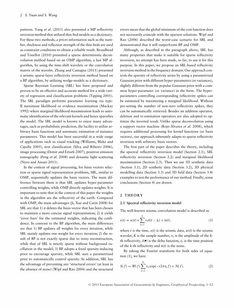
We designed a sparse reflectivity series (the leftmost trace inFig. 3) consisting in 701 reflectivity values with a sample in-terval of 1 ms, including 21 non-zero spikes and 680 zerovalues. The time positions and amplitudes of the 21 non-zeroreflectivity spikes are shown in the 1st column of the left paneland the 1st column of the right panel in Table 1, respectively.In order to test how well the method estimates weak reflec-tion, we set the minimum amplitude of the non-zero spikes as0.03, at a time position of 470 ms. In order to test the reso-lution of the method, we set the vertical two-way traveltimeof the thinnest bed as 8 ms, from 172–180 ms. By convolvinga 30 Hz Ricker wavelet with the designed reflectivity series,we generate a synthetic trace (the black continuous line in the82nd trace of Fig. 1) with a sample interval of 1 ms.

For the purpose of illustrating the working of the SSBLRImethod, we first illustrate how the inverted reflectivity seriesevolves with the iterations in Fig. 1. In this example, we set theinitial noise variance σ 2 as 0.009 and select the 5–70 Hz fre-quency band with a sample interval of 1 Hz to implement theinversion. As the figure shows, after the 1st iteration, there isonly a spike with the largest amplitude resolved. As iterationscontinue, the spikes with larger amplitude are first resolvedand then those with smaller amplitudes follow. In addition, inthe first 21 iterations, each iteration only resolves one spikeand the 21st iteration resolves the smallest one. The 2nd col-

Table 1 Time positions (the left panel) and amplitudes (the rightpanel) of the true, estimated in the 21st iteration and finally invertednon-zero reflectivity spikes. The four blue bold rows denote that theestimated reflectivity spikes could be re-updated during the iterations.Without imposing constraints on the numbers and time positionsof non-zero reflectivity spikes, the top or bottom of layers can beaccurately retrieved.

Time position Amplitude

True (ms) 21st Finally 21st Finally(ms) estimated inverted True estimated inverted

40 40 40 0.0750 0.0744 0.073360 60 60 0.1100 0.1084 0.109097 97 97 −0.0400 −0.0346 −0.0367138 138 138 0.1000 0.1005 0.0989172 171 172 0.1300 0.1232 0.1290180 181 180 −0.0900 −0.0802 −0.0886223 222 223 0.0850 0.0827 0.0834261 261 261 0.1400 0.1403 0.1390290 290 290 −0.0500 −0.0467 −0.0473337 336 337 0.0800 0.0734 0.0780350 350 350 0.0800 0.0706 0.0780390 390 390 −0.1000 −0.1006 −0.0992419 419 419 0.1300 0.1275 0.1284470 470 470 0.0300 0.0258 0.0263480 480 480 −0.0950 −0.0958 −0.0951530 530 530 0.0500 0.0479 0.0472570 570 570 −0.0700 −0.0694 −0.0688580 580 580 0.0700 0.0669 0.0680610 610 610 −0.2000 −0.1996 −0.1994640 640 640 0.1500 0.1494 0.1491660 660 660 0.0600 0.0577 0.0577

umn of the left panel and that of the right panel in Table 1 aretime positions and amplitudes of the inverted non-zero spikesduring the 21st iteration, respectively. In the 22nd and subse-quent iterations, the inverted non-zero spikes are re-updatedby an addition, deletion or re-estimation operator (see alsoTable 1). The 3rd column of the left panel and that of the rightpanel in Table 1 are the finally inverted non-zero reflectivityresults, also shown in the 82nd trace of Fig. 1. Compared withthe seismic trace (the black continuous line in the 82nd trace ofFig. 1), we observe that the retrieved reflectivity spikes at 172ms, 180 ms, 470 ms, 570 ms and 580 ms are not consistentwith the seismic peaks or troughs. That is to say, directly pick-ing peaks or troughs of seismic events to interpret the top orbottom of layers is probably not accurate, especially for thinlayers. However, SSBLRI accurately delineates the layers. Be-sides the time positions, the amplitudes of inverted reflectivityspikes are almost consistent with the true model.



Figure 1 How the inverted reflectivity series evolves iteration-by-iteration. The finally inverted reflectivity series and the original syn-thetic seismic trace are shown in the 82nd trace. The non-zero spikesare recovered one by one in the first 21 iterations. Moreover, the largespikes are first resolved. It is worth noting that the inverted non-zeroreflectivity spikes at 172 ms, 180 ms, 470 ms, 570 ms and 580 ms arenot consistent with the seismic peaks or troughs.

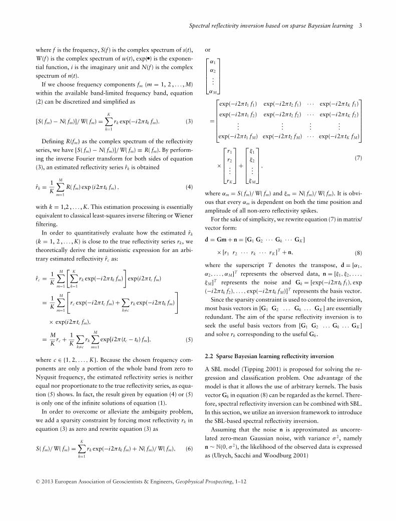
Figure 2 Wavelets with different phase errors compared with the truewavelet. The wavelet denoted by the arrow is the true 30 Hz Rickerwavelet.

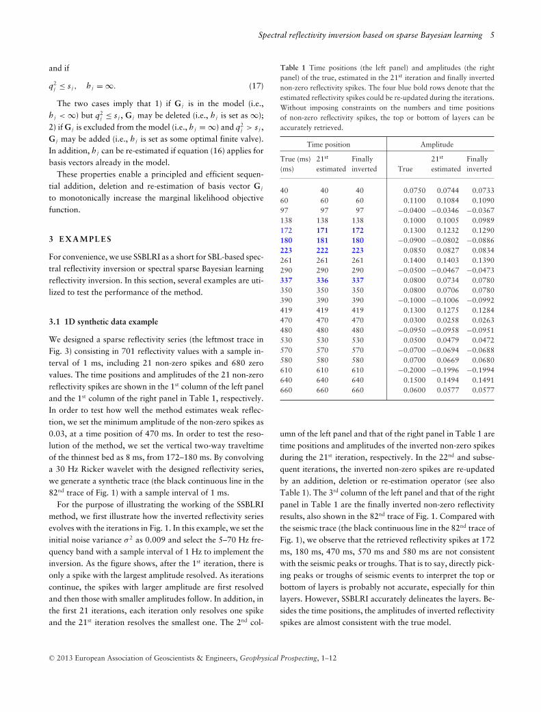
We then undertook a sensitivity study of the method withregards to the accuracy of the seismic wavelet. For conve-nience, we assume that the estimated wavelet only has a con-stant phase error compared with the true wavelet, which isdenoted by the arrow in Fig. 2. All the other wavelets in Fig. 2have a constant phase error with respect to the true wavelet.The inverted reflectivity spikes derived by using every waveletin Fig. 2 are shown in Fig. 3. It can be observed that if the phaseerror between the estimated wavelet and the true wavelet isnot more than 30◦, the inverted result is acceptable. In partic-ular, when the error is not more than 10◦, the inverted resultis almost the same as the true model. However, when theerror is more than 30◦, not only are false reflectivity valuesintroduced into the series but also the true reflectivity values

Figure 3 The true reflectivity series (the leftmost trace) and the in-verted reflectivity series using every wavelet in Fig. 2, respectively.

are distorted. That is to say, the accuracy of the wavelet is animportant factor for the SSBLRI method.

3.2 2D synthetic data example

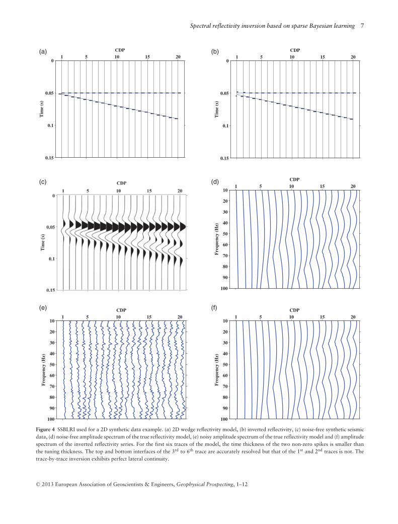
To test how well the SSBLRI method can identify thin bedsfrom a noisy data set, we generate a wedge model (Fig. 4a).The reflectivity of the top and bottom of the model are set as0.1 and –0.1, respectively. In the 1st trace (CDP number = 1),the vertical two-way traveltime between the top and bottomis 2 ms. As the CDP number increases, the two-way traveltimeincreases with a step of 2 ms. The long blue lines in Fig. 4(a)denote the top and bottom interfaces and the short black linesdenote the reflectivity. By convolving the reflectivity with a30 Hz Ricker wavelet, we obtain synthetic seismic data (Fig.4c) with a sample interval of 1 ms. According to Chung andLawton (1995), the tuning thickness of this model is approx-imately 13 ms.

Figure 4(d) is the amplitude spectrum of the true reflectivitymodel with a sample interval of 1 Hz. In the figure, every traceis a harmonic wave whose period is the inverse of the timethickness of the layer in this trace. This is the key idea of usingspectral decomposition (Partyka, Gridley and Lopez 1999) todetermine the thickness of a thin bed. In order to test whetherSSBLRI is robust to noise, 20% (S/N = 5:1, defined as the ratioof the complex spectrum energy of the true reflectivity modelto that of the noise in this paper) Gaussian noise is added tothe complex spectrum of the true reflectivity model within thefrequency band 10–100 Hz. As the amplitude spectrum in Fig.4(e) shows, due to the noise, there are no obvious spectrumpeaks or troughs to help determine the tuning thickness. Even



Figure 4 SSBLRI used for a 2D synthetic data example. (a) 2D wedge reflectivity model, (b) inverted reflectivity, (c) noise-free synthetic seismicdata, (d) noise-free amplitude spectrum of the true reflectivity model, (e) noisy amplitude spectrum of the true reflectivity model and (f) amplitudespectrum of the inverted reflectivity series. For the first six traces of the model, the time thickness of the two non-zero spikes is smaller thanthe tuning thickness. The top and bottom interfaces of the 3rd to 6th trace are accurately resolved but that of the 1st and 2nd traces is not. Thetrace-by-trace inversion exhibits perfect lateral continuity.



Figure 5 The relative error versus CDP number. The black line withcircles is the original relative error and the blue line with triangles isthe relative error magnified by 100 times from CDP 3–CDP 6.

if the time interval of the two non-zero spikes is relativelylarge, in, for example, the 20th trace, it is still difficult to findthe clear shape of the harmonic wave.

We set σ 2 for every trace as 0.03 and undertake a trace-by-trace reflectivity inversion. The inverted result is shown inFig. 4(b). To quantitatively evaluate the inverted result, wedefine the relative error as

∑Kk=1 (rk − rk)2/

∑Kk=1 r2

k , shownin Fig. 5. As Figs 4(b) and 5 show, the top and bottom in-terfaces of the 3rd to 20th trace are perfectly identified. Forthe 1st and 2nd trace, the relative error mainly results fromthe inaccurate inversion of the time positions of the two non-zero spikes. For the 3rd to 20th trace, the small relative errormainly results from inaccurate inversion of the amplitudes ofthe spikes, partially because of the influence of noise. Althoughthe reflectivity model is inverted trace-by-trace and there areno constraints imposed on the time positions and number oflayers, the lateral continuity of the inverted result is preservedwell and no visible false reflectivity spikes are introduced. Fig-ure 4(f) is the amplitude spectrum of the inverted reflectivity

model. Compared with Fig. 4(e), every trace in Fig. 4(f) issmoother and almost identical to the amplitude spectrum ofthe true reflectivity model (Fig. 4d).

3.3 3D physical modelling data example

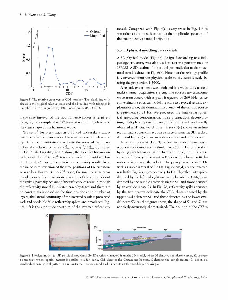
A 3D physical model (Fig. 6a), designed according to a fieldgeology structure, was also used to test the performance ofSSBLRI. A 2D section of the model perpendicular to the struc-tural trend is shown in Fig. 6(b). Note that the geology profileis converted from the physical scale to the seismic scale byusing the proportion 1:5000.

A seismic experiment was modelled in a water tank using amulti-channel acquisition system. The sources are ultrasonicwave transducers with a peak frequency of 260 kHz. Afterconverting the physical modelling scale to a typical seismic ex-ploration scale, the dominant frequency of the seismic sourceis equivalent to 26 Hz. We processed the data using spher-ical spreading compensation, noise attenuation, deconvolu-tion, multiple suppression, migration and stack and finallyobtained a 3D stacked data set. Figure 7(a) shows an in-linesection and a cross-line section extracted from the 3D stackeddata and Fig. 7(c) shows an in-line section and a time slice.

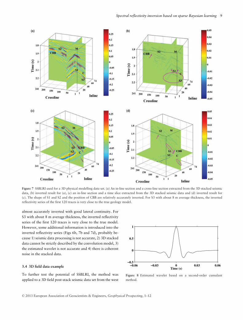
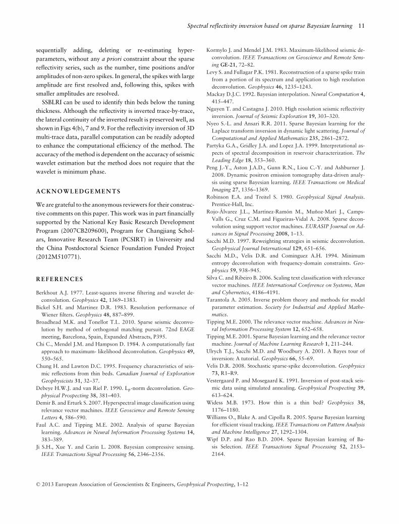
A seismic wavelet (Fig. 8) is first estimated based on asecond-order cumulant method. Then SSBLRI is undertakenby using parallel computation. In this example, the initial noisevariance for every trace is set as 0.5×var(d), where var( �) de-notes variance and the selected frequency band is 5–70 Hzwith a sample interval of 0.5 Hz. Figure 7(b,d) are the invertedresults for Fig. 7(a,c), respectively. In Fig. 7b, reflectivity spikesdenoted by the left and right arrows delineate the CBB, thosedenoted by the middle arrow delineate S1, and those denotedby an oval delineate S3. In Fig. 7d, reflectivity spikes denotedby the two arrows delineate the CBB, those denoted by theupper oval delineate S1, and those denoted by the lower ovaldelineate S3. As the figures show, the shape of S1 and S2 arerelatively accurately characterized. The position of the CBB is

Figure 6 Physical model. (a) 3D physical model and (b) 2D section extracted from the 3D model, where M denotes a mudstone layer, S2 denotesa sandbody whose spatial pattern is similar to a fan delta, CBB denotes the Cretaceous bottom, C denotes the conglomerate, S1 denotes asandbody whose spatial pattern is similar to the riverway sand and S3 denotes a thin sand-layer bearing oil.



Figure 7 SSBLRI used for a 3D physical modelling data set. (a) An in-line section and a cross-line section extracted from the 3D stacked seismicdata, (b) inverted result for (a), (c) an in-line section and a time slice extracted from the 3D stacked seismic data and (d) inverted result for(c). The shape of S1 and S2 and the position of CBB are relatively accurately inverted. For S3 with about 8 m average thickness, the invertedreflectivity series of the first 120 traces is very close to the true geology model.

almost accurately inverted with good lateral continuity. ForS3 with about 8 m average thickness, the inverted reflectivityseries of the first 120 traces is very close to the true model.However, some additional information is introduced into theinverted reflectivity series (Figs 6b, 7b and 7d), probably be-cause 1) seismic data processing is not accurate, 2) 3D stackeddata cannot be strictly described by the convolution model, 3)the estimated wavelet is not accurate and 4) there is coherentnoise in the stacked data.

3.4 3D field data example

To further test the potential of SSBLRI, the method wasapplied to a 3D field post-stack seismic data set from the west

Figure 8 Estimated wavelet based on a second-order cumulantmethod.



Figure 9 SSBLRI used for a 3D field data set. (a) An in-line section extracted from the 3D field data, (b) inverted result for (a), (c) a cross-linesection extracted from the 3D field data and (d) inverted result for (c).

Figure 10 Estimated wavelet based on a bispectral wavelet estimationmethod.

of China, that consists in 556 × 801 traces with a time sampleinterval of 2 ms. An in-line section and a cross-line section aredisplayed in Fig. 9(a,c), respectively.

A mixed-phase wavelet, shown in Fig. 10, is first estimatedbased on a bispectral wavelet estimation method (Yu et al.

2011). At this point, SSBLRI is implemented by using parallelcomputation. In this example, the initial noise variance forevery trace is set as 0.02×var(d) and the selected frequencyband is 5–65 Hz with a sample interval of 0.5 Hz. Figure9(b,d) are the inverted results for Fig. 9(a,c), respectively. AsFig. 9 shows, compared with the original seismic data, theinverted reflectivity has higher resolution with more details(marked with ovals). Furthermore, the relative amplitude andlateral continuity of the reflectivity are preserved well. Someweak reflections in the seismic data are emphasized.

CONCLUSIONS

The spectral sparse Bayesian learning reflectivity inversionmethod we present can be used to obtain a reliable, sparsereflectivity series with sparsity assumption about the re-flectivity. The method inverts for reflectivity spikes by



sequentially adding, deleting or re-estimating hyper-parameters, without any a priori constraint about the sparsereflectivity series, such as the number, time positions and/oramplitudes of non-zero spikes. In general, the spikes with largeamplitude are first resolved and, following this, spikes withsmaller amplitudes are resolved.

SSBLRI can be used to identify thin beds below the tuningthickness. Although the reflectivity is inverted trace-by-trace,the lateral continuity of the inverted result is preserved well, asshown in Figs 4(b), 7 and 9. For the reflectivity inversion of 3Dmulti-trace data, parallel computation can be readily adoptedto enhance the computational efficiency of the method. Theaccuracy of the method is dependent on the accuracy of seismicwavelet estimation but the method does not require that thewavelet is minimum phase.

ACKNOWLEDGE ME N T S

We are grateful to the anonymous reviewers for their construc-tive comments on this paper. This work was in part financiallysupported by the National Key Basic Research DevelopmentProgram (2007CB209600), Program for Changjiang Schol-ars, Innovative Research Team (PCSIRT) in University andthe China Postdoctoral Science Foundation Funded Project(2012M510771).

REFERENCES

Berkhout A.J. 1977. Least-squares inverse filtering and wavelet de-convolution. Geophysics 42, 1369–1383.

Bickel S.H. and Martinez D.R. 1983. Resolution performance ofWiener filters. Geophysics 48, 887–899.

Broadhead M.K. and Tonellot T.L. 2010. Sparse seismic deconvo-lution by method of orthogonal matching pursuit. 72nd EAGEmeeting, Barcelona, Spain, Expanded Abstracts, P395.

Chi C., Mendel J.M. and Hampson D. 1984. A computationally fastapproach to maximum- likelihood deconvolution. Geophysics 49,550–565.

Chung H. and Lawton D.C. 1995. Frequency characteristics of seis-mic reflections from thin beds. Canadian Journal of ExplorationGeophysicists 31, 32–37.

Debeye H.W.J. and van Riel P. 1990. Lp-norm deconvolution. Geo-physical Prospecting 38, 381–403.

Demir B. and Erturk S. 2007. Hyperspectral image classification usingrelevance vector machines. IEEE Geoscience and Remote SensingLetters 4, 586–590.

Faul A.C. and Tipping M.E. 2002. Analysis of sparse Bayesianlearning. Advances in Neural Information Processing Systems 14,383–389.

Ji S.H., Xue Y. and Carin L. 2008. Bayesian compressive sensing.IEEE Transactions Signal Processing 56, 2346–2356.

Kormylo J. and Mendel J.M. 1983. Maximum-likelihood seismic de-convolution. IEEE Transactions on Geoscience and Remote Sens-ing GE-21, 72–82.

Levy S. and Fullagar P.K. 1981. Reconstruction of a sparse spike trainfrom a portion of its spectrum and application to high resolutiondeconvolution. Geophysics 46, 1235–1243.

Mackay D.J.C. 1992. Bayesian interpolation. Neural Computation 4,415–447.

Nguyen T. and Castagna J. 2010. High resolution seismic reflectivityinversion. Journal of Seismic Exploration 19, 303–320.

Nyeo S.-L. and Ansari R.R. 2011. Sparse Bayesian learning for theLaplace transform inversion in dynamic light scattering. Journal ofComputational and Applied Mathematics 235, 2861–2872.

Partyka G.A., Gridley J.A. and Lopez J.A. 1999. Interpretational as-pects of spectral decomposition in reservoir characterization. TheLeading Edge 18, 353–360.

Peng J.-Y., Aston J.A.D., Gunn R.N., Liou C.-Y. and Ashburner J.2008. Dynamic positron emission tomography data-driven analy-sis using sparse Bayesian learning. IEEE Transactions on MedicalImaging 27, 1356–1369.

Robinson E.A. and Treitel S. 1980. Geophysical Signal Analysis.Prentice-Hall, Inc.

Rojo-Alvarez J.L., Martınez-Ramon M., Munoz-Marı J., Camps-Valls G., Cruz C.M. and Figueiras-Vidal A. 2008. Sparse decon-volution using support vector machines. EURASIP Journal on Ad-vances in Signal Processing 2008, 1–13.

Sacchi M.D. 1997. Reweighting strategies in seismic deconvolution.Geophysical Journal International 129, 651–656.

Sacchi M.D., Velis D.R. and Cominguez A.H. 1994. Minimumentropy deconvolution with frequency-domain constraints. Geo-physics 59, 938–945.

Silva C. and Ribeiro B. 2006. Scaling text classification with relevancevector machines. IEEE International Conference on Systems, Manand Cybernetics, 4186–4191.

Tarantola A. 2005. Inverse problem theory and methods for modelparameter estimation. Society for Industrial and Applied Mathe-matics.

Tipping M.E. 2000. The relevance vector machine. Advances in Neu-ral Information Processing System 12, 652–658.

Tipping M.E. 2001. Sparse Bayesian learning and the relevance vectormachine. Journal of Machine Learning Research 1, 211–244.

Ulrych T.J., Sacchi M.D. and Woodbury A. 2001. A Bayes tour ofinversion: A tutorial. Geophysics 66, 55–69.

Velis D.R. 2008. Stochastic sparse-spike deconvolution. Geophysics73, R1–R9.

Vestergaard P. and Mosegaard K. 1991. Inversion of post-stack seis-mic data using simulated annealing. Geophysical Prospecting 39,613–624.

Widess M.B. 1973. How thin is a thin bed? Geophysics 38,1176–1180.

Williams O., Blake A. and Cipolla R. 2005. Sparse Bayesian learningfor efficient visual tracking. IEEE Transactions on Pattern Analysisand Machine Intelligence 27, 1292–1304.

Wipf D.P. and Rao B.D. 2004. Sparse Bayesian learning of Ba-sis Selection. IEEE Transactions Signal Processing 52, 2153–2164.



Wipf D.P. and Rao B.D. 2006. Comparing the effects of differentweight distributions on finding sparse representations. Advances inNeural Information Processing Systems 18.

Yang H., Zheng X.D., Ma S.F. and Li J.S. 2011. Thin-bed reflectiv-ity inversion based on matching pursuit. 81st SEG meeting, SanAntonio, Texas, Expanded Abstracts, 2586–2590.

Yu Y.C., Wang S.X., Yuan S.Y. and Qi P.F. 2011. Phase estimationin bispectral domain based on conformal mapping and applicationsin seismic wavelet estimation. Applied Geophysics 8, 36–47.

Yuan S.Y., Wang S.X. and Li G.F. 2012. Random noise reductionusing Bayesian inversion. Journal of Geophysics and Engineering9, 60–68.

Yuan S.Y., Wang S.X. and Tian N. 2009. Swarm intelligence opti-mization and its application in geophysical data inversion. AppliedGeophysics 6, 166–174.

Zhang R. and Castagna J. 2011. Seismic sparse-layer reflectiv-ity inversion using basis pursuit decomposition. Geophysics 76,R147–R158.


spectral sparse bayesian learning reflectivity inversion...

Documents