spectrum sensing techniques for cognitive radio...

Spectrum Sensing Techniques for Cognitive Radio

Applications

A Thesis

Submitted for the Degree of

Doctor of Philosophy

in the Faculty of Engineering

Submitted by

Sanjeev G.

Electrical Communication Engineering

Indian Institute of Science, Bangalore

Bangalore – 560 012 (INDIA)

January 2015

TO

My parents

Smt. Shakunthala Aggithala Padmanabha

and

Sri. Gurugopinath Sanjeeva Rao

Acknowledgements

!"#$%&'()*

! "#$%&

!"!#$

!"#$%&'($ )*

i

Acknowledgements ii

!"#$% # &'()*#+,

!"#$%&'()*+,-.

! "!# # $%" &' () )"

In the above stanzas,1 I acknowledge and salute Saraswathi, the Goddess of Learning,

my mentor Chandra Murthy, my family: my parents, brother, and wife, my philosoph-

ical and spiritual guides D. V. Gundappa, K. Krishnamoorthy and M. Krishnamurti,

Shannon, the Father of Information Theory, Shatavadhani R. Ganesh, my thesis exam-

iners Marceau Coupechoux and Mohammed Zafar Ali Khan.

1This piece of poetry, called as the Kanda Padya, is based on an ancient form of Chandas (metre),used in Kannada by 10th Century poets such as Pampa, Ranna, Ponna to the 21st Century poets such asBasavappa Shastry, D. V. Gundappa and R. Ganesh. Interested readers can refer to the following referencefor more information on its aesthetic details.S. Krishna Bhatta, “Sediyapu Chandassamputa,” 1st ed., Rastrakavi Govinda Pai Samshodhana Kendra,2006.

Acknowledgements iii

I would like to express my gratitude to my adviser, Prof. Chandra R. Murthy, without

whom this work would not have been possible. During the kindergarten days of my

research life, he taught me to walk with confidence, helped me stand up whenever

I fell, and even carried me when I could not walk. It is seldom that one finds a man,

who is punctual, diligent, a well-prepared teacher, does A-grade quality research work,

and does it with both his feet on the ground. His dedication towards preparing for his

lectures and presentations have simply stunned me over all these years. All the well-

constructed sentences in this thesis are due to him; either directly or indirectly. I have

learnt about the art of research, and a lot of presentation, teaching, and social skills

from him. Thanks for everything, Chandra.

I thank the Director of the Indian Institute of Science, and the Chairman of the ECE

department, for giving me an opportunity to work in this esteemed institution. Thanks

to the funding from the Ministry of Human Resource Development, Government of

India, for providing me rice, sambar and shelter throughout my stay here.

I thank the Govt. of India, Aerospace Network Research Consortium (ANRC), IEEE

Globecom student travel grant, SPCOM student travel grant, and directorate of extra-

mural research and intellectual property rights, Defence Research and Development

Organization (DRDO), Govt. of India, for their financial support for my research.

I would like to thank all my co-authors and collaborators, especially Prof. Vinod

Sharma, Prof. Chandra Sekhar Seelamantula, and Prof. Bharadwaj Amrutur.

I thank my teachers Profs. Chandra Murthy, Neelesh Mehta, Rajesh Sundaresan, Ut-

pal Mukherjee, Anurag Kumar, A. Chokalingam, K. V. S. Hari, Chandra Sekhar Seela-

mantula, Vinod Sharma, M. K. Ghosh, and S. K. Iyer, for providing insights into the

respective courses that they taught.

Heartfelt thanks to my dear friends Bharath, Nagananda, Deepa, Chandrashekar,

Ganesan, J. Chandrasekhar, Krishna Chaythanya, Srinivas Reddy, Venugopalakrishna,

Parthajit, Ranjitha, Abhay, Santhosh Kumar, Suma, Raghavendra, Anup, Reuben,Manesh,

Sinchu, Karthik Velugoori, Sneha Latha and others for making my stay a memorable

one. God bless everyone. Special thanks to pals Bharath and Nagananda for all the

timely visits to Vidyarthi Bhavan, Ranjitha and Abhay for the memorable trips and

treks, Venu and Parthajit for the philosophical discussions, and Venu for all the valu-

able time spent at GIPA. Also, sincere thanks to my friends from the other labs and

Acknowledgements iv

departments Karthik A., Gautam, Vijesh Joshi, Ashok, Harshan, Naveen K. P., Srinidhi,

Harshavardhan, Naveen Deshpande, Shubha, Raghava, and Aditya Roychoudhury.

I thank various clubs in IISc that I was a part of. First off, I thank the Music Club

for providing me with an opportunity to be the Convener for an year. Rhythmica, the

official IISc band, has givenme a lot of friends, and a rare opportunity to work with 50+

talented musicians all across the campus. Thanks, fellas! I would also like to thank the

kung-fu, tennis and badminton clubs for giving me fun-filled days to cherish forever.

Interactions with my friends from the lab and Rhythmica at eat outlets in the campus

such as the coffee board, tea kiosk, Prakruthi, Kabini canteen, Nesara, and gym-cafe

have been very fruitful. Breakfast, lunch and dinner sessions in A-mess were awesome!

I thank all the managing and helping hands in these places.

I would like to express my gratitude to the staff at the ECE dept. office for making my

life simpler by directing me to the correct places to get all my administration-related

work done smoothly. Thanks to the staff at the main hostel office, and the U-block

office for their support, especially on the day when I had to break open the lock of

my room! My sincere thanks and appreciation goes to the chief security officer Mr.

Chandrasekhar, and staff at the security office, who work day and night to keep the

campus safe for the residents.

Finally, my heartfelt thanks tomy Father, Sri. Gurugopinath, myMother, Smt. Shakun-

thala for providing me the opportunity to pursue my dreams while they toiled day and

night. In the age when the entire race shifted its attention to the software industry, my

Father believed in my teaching abilities and has taken all the financial responsibilities

so that I could work in peace. My little brother, Sri. Rajiv, has taken a lot of responsibil-

ities from my shoulders, and has done a great job, without complaining. My blessings

are with him. The latest entry into my life, Shwetha, my wife has taken a very brave

decision to marry a research student on stipend, and has sacrificed a lot of her small

fun filled moments for my research. Thanks, everyone!

Abstract

Cognitive Radio (CR) has received tremendous research attention over the past decade,

both in the academia and industry, as it is envisioned as a promising solution to the

problem of spectrum scarcity. A CR is a device that senses the spectrum for occupancy

by licensed users (also called as primary users), and transmits its data only when the

spectrum is sensed to be available. For the efficient utilization of the spectrum while

also guaranteeing adequate protection to the licensed user from harmful interference,

the CR should be able to sense the spectrum for primary occupancy quickly as well

as accurately. This makes Spectrum Sensing (SS) one of the fundamental blocks in the

operation of a CR. At its core, SS is a hypothesis testing problem, where the goal is

to test whether the primary user is inactive (the null or noise-only hypothesis), or not

(the alternate or signal-present hypothesis). Computational simplicity, robustness to

uncertainties in the knowledge of various noise, signal, and fading parameters, and

ability to handle interference or other source of non-Gaussian noise are some of the

desirable features of a SS unit in a CR.

In many practical applications, CR devices can exploit known structure in the pri-

mary signal. In the IEEE 802.22 CR standard, the primary signal is a wideband signal,

but with a strong narrowband pilot component. In other applications, such as mil-

itary communications, and bluetooth, the primary signal uses a Frequency Hopping

(FH) transmission. These applications can significantly benefit from detection schemes

that are tailored for detecting the corresponding primary signals. This thesis develops

novel detection schemes and rigorous performance analysis of these primary signals

in the presence of fading. For example, in the case of wideband primary signals with

a strong narrowband pilot, this thesis answers the further question of whether to use

the entire wideband for signal detection, or whether to filter out the pilot signal and

v

Abstract vi

use narrowband signal detection. The question is interesting because the fading char-

acteristics of wideband and narrowband signals are fundamentally different. Due to

this, it is not obvious which detection scheme will perform better in practical fading

environments.

At another end of the gamut of SS algorithms, when the CR has no knowledge of the

structure or statistics of the primary signal, and when the noise variance is known, En-

ergy Detection (ED) is known to be optimal for SS. However, the performance of the ED

is not robust to uncertainties in the noise statistics or under different possible primary

signal models. In this case, a natural way to pose the SS problem is as a Goodness-of-

Fit Test (GoFT), where the idea is to either accept or reject the noise-only hypothesis.

This thesis designs and studies the performance of GoFTs when the noise statistics can

even be non-Gaussian, and with heavy tails. Also, the techniques are extended to the

cooperative SS scenario where multiple CR nodes record observations using multiple

antennas and perform decentralized detection.

In this thesis, we study all the issues listed above by considering both single and

multiple CR nodes, and evaluating their performance in terms of (a) probability of de-

tection error, (b) sensing-throughput tradeoff, and (c) probability of rejecting the null-

hypothesis. We propose various SS strategies, compare their performance against exist-

ing techniques, and discuss their relative advantages and performance tradeoffs. The

main contributions of this thesis are as follows:

• The question of whether to use pilot-based narrowband sensing or wideband

sensing is answered using a novel, analytically tractable metric proposed in this

thesis called the error exponent with a confidence level.

• Under a Bayesian framework, obtaining closed form expressions for the optimal

detection threshold is difficult. Near-optimal detection thresholds are obtained

for most of the commonly encountered fading models.

• For an FH primary, using the Fast Fourier Transform (FFT) Averaging Ratio (FAR)

algorithm, the sensing-throughput tradeoff are derived in closed form.

• A GoFT technique based on the statistics of the number of zero-crossings in the

observations is proposed, which is robust to uncertainties in the noise statistics,

Abstract vii

and outperforms existing GoFT-based SS techniques.

• A multi-dimensional GoFT based on stochastic distances is studied, which pro-

vides better performance compared to some of the existing techniques. A special

case, i.e., a test based on the Kullback-Leibler distance is shown to be robust to

some uncertainties in the noise process.

All of the theoretical results are validated using Monte Carlo simulations. In the case

of FH-SS, an implementation of SS using the FAR algorithm on a commercially off-the-

shelf platform is presented, and the performance recorded using the hardware is shown

to corroborate well with the theoretical and simulation-based results. The results in this

thesis thus provide a bouquet of SS algorithms that could be useful under different CR-

SS scenarios.

Glossary

ADC : Analog-to-Digital ConverterADD : Anderson-Darling statistic based DetectorAR : Auto RegressiveARMA : Auto Regressive Moving AverageAWGN : Additive White Gaussian Noise

B : Bhattacharyya DistanceBD : Blind DetectorBPF : Band Pass Filter

CCDF : Complementary CDFCDF : Cumulative Distribution FunctionCFAR : Constant False Alarm RateCLT : Central Limit TheoremCR : Cognitive Radio

DAC : Digital-to-Analog ConverterDCM : Data Conversion ModuleDP : Development PlatformDPM : Digital Processing ModuleDSP : Digital Signal ProcessingDTV : Digital Tele-Vision

ED : Energy DetectionEECL : Error Exponent with a Confidence LevelER : Eigenvalue Ratio based Test

FAR : FFT Averaging RatioFC : Fusion CenterFDMA : Frequency Division Multiple AccessFFT : Fast Fourier TransformFH : Frequency-HoppingFPGA : Field-Programmable Gate Array

viii

Glossary ix

GoFT : Goodness-of-Fit TestGUI : Graphical User Interface

H : Hellinger DistanceHOC : Higher Order Crossings

ID : Interpoint DistanceIEEE : Institute of Electrical and Electronics EngineersIF : Intermediate Frequencyi.i.d. : Independent and Identically Distributed

KL : Kullback-Leibler Distance

LC : Level-CrossingsLR : Likelihood Ratio

MA : Moving AverageMAC : Medium Access Control LayerMBDK : Model Based Design KitMDGoFT : Multi-Dimensional GoFT

NB : Narrow-BandNCO : Numerically Controlled OscillatorNP : Neyman-PearsonNPU : Noise Parameter UncertaintyNMU : Noise Model UncertaintyNVU : Noise Variance Uncertainty

OSD : Ordered Statistics based Detector

PDF : Probability Density FunctionPHY : Physical LayerP-IV : Pearson type IV distributionPN : Psuedo-randomΨ1SD : ΨwSD with uniform and equal weightsΨeSD : ΨwSD with exponential weightsΨwSD : Ψ2 Statistic based DetectorPU : Primary User

QoS : Quality-of-ServiceQPSK : Quadrature Phase Shift Keying

RF : Radio-FrequencyRFM : RF Module

Glossary x

SαS : Symmetric-α Stable DistributionSFF : Small Form FactorSDR : Software Defined RadioSNR : Signal-to-Noise RatioSS : Spectrum SensingST : Sphericity TestSTFT : Short Time Fourier Transform

TDMA : Time Division Multiple Access

VHP : Virtual Hopping PeriodVPBE : Video Processing Back EndVPFE : Video Processing Front EndVPSS : Video Processing Sub-System

WB : Wide-BandWBX : Wide Bandwidth TransceiverWRAN : Wireless Regional Area NetworkWZCD : Weighted Zero-Crossings Detector

ZC : Zero-Crossings

Contents

Acknowledgements i

Abstract v

Glossary viii

1 Introduction 1

1.1 Spectrum Sensing . . . . . . . . . . . . . . . . . . . . . . . . . . . . . . . . 2

1.2 Scenarios for Spectrum Sensing . . . . . . . . . . . . . . . . . . . . . . . . 3

1.2.1 Available Knowledge About the Primary Signal . . . . . . . . . . 4

1.2.2 Signal Acquisition Scenarios . . . . . . . . . . . . . . . . . . . . . 6

1.2.3 Performance Criteria and Problem Formulation . . . . . . . . . . 6

1.2.4 Multi-Sensor Detection . . . . . . . . . . . . . . . . . . . . . . . . . 7

1.3 Challenges in Spectrum Sensing . . . . . . . . . . . . . . . . . . . . . . . 8

1.3.1 Effect of Fading . . . . . . . . . . . . . . . . . . . . . . . . . . . . . 8

1.3.2 Frequency-Hopping Primary Signals . . . . . . . . . . . . . . . . 10

1.3.3 Robustness to Noise Models . . . . . . . . . . . . . . . . . . . . . 10

1.4 Contributions of the Thesis . . . . . . . . . . . . . . . . . . . . . . . . . . 11

2 Error Exponent Analysis of Energy-Based Bayesian Decentralized Spectrum

Sensing Under Fading 17

2.1 Introduction . . . . . . . . . . . . . . . . . . . . . . . . . . . . . . . . . . . 17

2.2 System Model . . . . . . . . . . . . . . . . . . . . . . . . . . . . . . . . . . 22

2.3 Detection at the Sensors . . . . . . . . . . . . . . . . . . . . . . . . . . . . 25

2.4 Detection at the Fusion Center . . . . . . . . . . . . . . . . . . . . . . . . . 28

xi

CONTENTS xii

2.4.1 Extension to Unequal Average Received Signal Powers . . . . . . 30

2.4.2 Lower Bounds on the EECL . . . . . . . . . . . . . . . . . . . . . . 31

2.4.3 Optimality of the OR rule . . . . . . . . . . . . . . . . . . . . . . . 32

2.5 Wideband Vs. Narrowband Spectrum Sensing . . . . . . . . . . . . . . . 32

2.5.1 NB vs. WB Sensing at Individual Sensors . . . . . . . . . . . . . . 33

2.5.2 NB vs. WB Sensing at the Fusion Center . . . . . . . . . . . . . . . 33

2.6 Numerical Results and Simulations . . . . . . . . . . . . . . . . . . . . . . 34

2.6.1 Detection at the Sensors . . . . . . . . . . . . . . . . . . . . . . . . 35

2.6.2 Detection at the Fusion Center . . . . . . . . . . . . . . . . . . . . 36

2.7 Conclusions . . . . . . . . . . . . . . . . . . . . . . . . . . . . . . . . . . . 40

3 Near-Optimal Detection Thresholds for Bayesian Spectrum Sensing 44

3.1 Introduction . . . . . . . . . . . . . . . . . . . . . . . . . . . . . . . . . . . 44

3.2 System Model . . . . . . . . . . . . . . . . . . . . . . . . . . . . . . . . . . 48

3.3 Detection Under Various Fading Models . . . . . . . . . . . . . . . . . . . 50

3.3.1 Detection Under Rayleigh Fading . . . . . . . . . . . . . . . . . . 50

3.3.2 Detection Under Lognormal Shadowing . . . . . . . . . . . . . . 51

3.3.3 Detection Under Nakagami-m Fading . . . . . . . . . . . . . . . . 53

3.3.4 Detection Under Weibull Fading . . . . . . . . . . . . . . . . . . . 54

3.4 Simulation Results . . . . . . . . . . . . . . . . . . . . . . . . . . . . . . . 57

3.5 Conclusions . . . . . . . . . . . . . . . . . . . . . . . . . . . . . . . . . . . 61

4 Design and Implementation of Spectrum Sensing with a Frequency-Hopping

Primary System 64

4.1 Introduction . . . . . . . . . . . . . . . . . . . . . . . . . . . . . . . . . . . 64

4.2 System Model and FAR Algorithm . . . . . . . . . . . . . . . . . . . . . . 67

4.2.1 System Model . . . . . . . . . . . . . . . . . . . . . . . . . . . . . . 67

4.2.2 The FAR algorithm . . . . . . . . . . . . . . . . . . . . . . . . . . . 70

4.3 Performance Analysis and Optimization . . . . . . . . . . . . . . . . . . . 71

4.3.1 Probabilities of False Alarm and Detection . . . . . . . . . . . . . 71

4.3.2 Optimum Sensing Duration . . . . . . . . . . . . . . . . . . . . . . 72

4.4 Results . . . . . . . . . . . . . . . . . . . . . . . . . . . . . . . . . . . . . . 75

4.4.1 Monte Carlo Simulations . . . . . . . . . . . . . . . . . . . . . . . 75

CONTENTS xiii

4.4.2 Experimental Results from the Lyrtech SFF SDR DP . . . . . . . . 78

4.5 Conclusions . . . . . . . . . . . . . . . . . . . . . . . . . . . . . . . . . . . 79

5 Zero-Crossings Based Spectrum Sensing Under Noise Uncertainties 84

5.1 Introduction . . . . . . . . . . . . . . . . . . . . . . . . . . . . . . . . . . . 84

5.2 System Model . . . . . . . . . . . . . . . . . . . . . . . . . . . . . . . . . . 87

5.3 Existing GoFT for Spectrum Sensing . . . . . . . . . . . . . . . . . . . . . 89

5.3.1 Energy Detector (ED) . . . . . . . . . . . . . . . . . . . . . . . . . . 89

5.3.2 Anderson-Darling Statistic Based Detector (ADD) . . . . . . . . . 90

5.3.3 Blind Detector (BD) . . . . . . . . . . . . . . . . . . . . . . . . . . . 91

5.4 Weighted Zero-Crossings Based Detection . . . . . . . . . . . . . . . . . . 92

5.5 Robustness to Noise Uncertainties . . . . . . . . . . . . . . . . . . . . . . 96

5.5.1 Noise Model Uncertainty . . . . . . . . . . . . . . . . . . . . . . . 96

5.5.2 Noise Parameter Uncertainty . . . . . . . . . . . . . . . . . . . . . 97

5.6 Expected HOCs for Correlated Gaussian Noise . . . . . . . . . . . . . . . 98


5.7.1 Performance Under I.I.D. Noise . . . . . . . . . . . . . . . . . . . 100

5.7.2 Performance Under Colored Noise . . . . . . . . . . . . . . . . . . 103

5.8 Probability of Detection for Constant Primary . . . . . . . . . . . . . . . . 104

5.9 Conclusion . . . . . . . . . . . . . . . . . . . . . . . . . . . . . . . . . . . . 107

6 Multi-dimensional Goodness-of-Fit Tests Based on Stochastic Distances For

Spectrum Sensing 112

6.1 Introduction . . . . . . . . . . . . . . . . . . . . . . . . . . . . . . . . . . . 112

6.2 System Model . . . . . . . . . . . . . . . . . . . . . . . . . . . . . . . . . . 114

6.3 Interpoint Distance Based GoFT . . . . . . . . . . . . . . . . . . . . . . . . 117

6.3.1 Choice of δ(·, ·) . . . . . . . . . . . . . . . . . . . . . . . . . . . . . 121

6.3.2 Extension to Multiple Sensors . . . . . . . . . . . . . . . . . . . . . 121

6.4 〈h, φ〉 Distance Based GoFT . . . . . . . . . . . . . . . . . . . . . . . . . . 122

6.4.1 Expressions for Various dhφ(·, ·) Distances . . . . . . . . . . . . . . 124

6.4.2 Robustness of the KL Distance Metric dKL(·, ·) . . . . . . . . . . . 125


6.5.1 ID Test . . . . . . . . . . . . . . . . . . . . . . . . . . . . . . . . . . 126

CONTENTS xiv

6.5.2 〈h, φ〉 Test . . . . . . . . . . . . . . . . . . . . . . . . . . . . . . . . 128

6.6 Conclusions . . . . . . . . . . . . . . . . . . . . . . . . . . . . . . . . . . . 129

7 Conclusions and Future Work 134

7.1 Contributions . . . . . . . . . . . . . . . . . . . . . . . . . . . . . . . . . . 134

7.2 Future Work . . . . . . . . . . . . . . . . . . . . . . . . . . . . . . . . . . . 136

A Appendix for Chapter 2 138

A.1 Proof of Theorem 1 . . . . . . . . . . . . . . . . . . . . . . . . . . . . . . . 138


A.3 Proof of Corollary 1 . . . . . . . . . . . . . . . . . . . . . . . . . . . . . . . 142

A.4 Proof of Corollary 2 . . . . . . . . . . . . . . . . . . . . . . . . . . . . . . . 143


A.6 Expressions for Approximations in Sec. 2.4, Cor. 1 . . . . . . . . . . . . . 145

A.6.1 Weibull Sum Approximation in Rayleigh Fading Case . . . . . . 145

A.6.2 Pearson Type IV Approximation in Lognormal Shadowing Case 147

B Appendix for Chapter 3 148

B.1 Proof of Theorem 4 . . . . . . . . . . . . . . . . . . . . . . . . . . . . . . . 148



B.4 Error Exponent at the FC using the K-out-of-N Rule . . . . . . . . . . . . 155

B.5 Detection Under Suzuki Fading . . . . . . . . . . . . . . . . . . . . . . . . 159

C Appendix for Chapter 4 161

C.1 Proof of Lemma 1 . . . . . . . . . . . . . . . . . . . . . . . . . . . . . . . . 161

C.2 Proof of Lemma 2 . . . . . . . . . . . . . . . . . . . . . . . . . . . . . . . . 162

C.3 FAR Algorithm on Lyrtech SFF SDR DP . . . . . . . . . . . . . . . . . . . 164

C.3.1 Primary Hop-Instant Identification . . . . . . . . . . . . . . . . . . 165

D Appendix for Chapter 5 170

D.1 Proof of Lemma 3 . . . . . . . . . . . . . . . . . . . . . . . . . . . . . . . . 170

D.2 Proof of Corollary 4 . . . . . . . . . . . . . . . . . . . . . . . . . . . . . . . 171

D.3 Analysis on the non-applicability of ADD and ED . . . . . . . . . . . . . 171

CONTENTS xv

D.4 On the Wider-Applicability of the Blind Detector . . . . . . . . . . . . . . 173

E Popular Goodness-of-Fit Tests For the Gaussian Distribution 176

E.1 Regression and Correlation Based Tests . . . . . . . . . . . . . . . . . . . 177

E.1.1 The W Test (Shapiro-Wilk Test) . . . . . . . . . . . . . . . . . . . . . 178

E.1.2 The Y Test (D’Agostino Test) . . . . . . . . . . . . . . . . . . . . . . 179

E.1.3 The Z Test . . . . . . . . . . . . . . . . . . . . . . . . . . . . . . . . 180

E.1.4 The QH* Test . . . . . . . . . . . . . . . . . . . . . . . . . . . . . . 181

E.1.5 The Q Test . . . . . . . . . . . . . . . . . . . . . . . . . . . . . . . . 181

E.2 Empirical Distribution Function (EDF) Based Tests . . . . . . . . . . . . . 183

E.2.1 The D Test (Kolmogorov-Smirnov Test) . . . . . . . . . . . . . . . . 183

E.2.2 The W2 Test (Cramer-Von Mises Test) . . . . . . . . . . . . . . . . . 184

E.2.3 The A2 Test (Anderson-Darling Test) . . . . . . . . . . . . . . . . . 185

E.3 Omnibus Tests . . . . . . . . . . . . . . . . . . . . . . . . . . . . . . . . . . 185

E.3.1 The K2 Test . . . . . . . . . . . . . . . . . . . . . . . . . . . . . . . 185

E.3.2 The G2w Test . . . . . . . . . . . . . . . . . . . . . . . . . . . . . . . 187

E.3.3 The G2∗w Test . . . . . . . . . . . . . . . . . . . . . . . . . . . . . . . 187

E.3.4 The L-Moment Skewness-Kurtosis (LSK) Based Test . . . . . . . . 188

Bibliography 189

List of Figures

1.1 Different Scenarios for Spectrum Sensing. . . . . . . . . . . . . . . . . . . 4

1.2 Contributions of the Thesis. . . . . . . . . . . . . . . . . . . . . . . . . . . 12

2.1 One sided PSD of IEEE 802.22 DTV wideband signal. . . . . . . . . . . . 21

2.2 CDF of W ,∑10

k=1 (eyk − 1)2, where yk are i.i.d. and truncated Gaussian

distributedwith (mean, variance)= (0.9, 0.165), (0.85, 0.15) and (0.5, 0.165),

and yk > 0 with probability 1. . . . . . . . . . . . . . . . . . . . . . . . . . 30

2.3 Trade-off between NB and WB sensing at a single sensor, with µs = 0 in

the WB case. . . . . . . . . . . . . . . . . . . . . . . . . . . . . . . . . . . . 36

2.4 Variation of pe with a confidence q as a function of SNR, under narrow-

band Rayleigh fading. Here, N = 1, π0 = 0.5, M = 106. The curve

labeled ’Mismatched τ ’ corresponds to using π0 = 0.5 to design the de-

tector, when the actual π0 = 0.01. . . . . . . . . . . . . . . . . . . . . . . . 37

2.5 Variation of the lower bound on ǫ(N)E as a function of PNB

PWB, with q = 0.99,

µs = 0, σs = 1. . . . . . . . . . . . . . . . . . . . . . . . . . . . . . . . . . . 38

2.6 Variation of ǫ(N)E as a function of PNB

PWB, with q = 0.99, µs = 0, σs = 1. . . . . 39

2.7 Variation of ǫ(N)E as a function of q, with N = 4, µs = 0, σs = 1. . . . . . . 40

2.8 Variation of ǫ(N)E as a function of N , with PNB

PWB= 1, µs = 0, σs = 1. . . . . . 41

2.9 Variation of PE with a confidence level as a function of PNB

PWBwith q = 0.99,

µs = 0, σs = 1 and π0 = 0.5. . . . . . . . . . . . . . . . . . . . . . . . . . . . 42

2.10 Comparison of the Bayesian and Neyman-Pearson approaches in terms

of the PE with a confidence q = 0.99, as a function of the average primary

SNR, with µs = 0, σs = 1 and π0 = 0.5. . . . . . . . . . . . . . . . . . . . . 42

xvi

LIST OF FIGURES xvii

3.1 CDF of Lognormal distribution for various values of its log-shape pa-

rameter, and the corresponding Normal CDF approximation. . . . . . . . 52

3.2 CCDF of Lognormal distribution for various values of its log-shape pa-

rameter, and the corresponding Normal CCDF approximation. . . . . . . 53

3.3 CDF of the Weibull distribution for various values of its scale and shape

parameters, and the corresponding Normal CDF approximation. . . . . 56

3.4 CCDF of theWeibull distribution for various values of its scale and shape

parameters, and the corresponding Normal CCDF approximation. . . . 57

3.5 Variation of x(R)CLT withM for the optimum and CLT schemes. . . . . . . . 58

3.6 A constant pe can be maintained if P√M remains fixed. . . . . . . . . . . 59

3.7 Simulated optimal thresholds and near-optimal theoretical thresholds

for the shadowing fading case, with its log-scale parameter σdB = 0.5. . . 60


for the Weibull fading case, with aw = 5, bw = 1. . . . . . . . . . . . . . . . 61


for the Nakagami-m fading case, with K = 10. . . . . . . . . . . . . . . . 62

3.10 Variation of ǫE with N (π0 = 0.5). . . . . . . . . . . . . . . . . . . . . . . . 63

3.11 Variation of PE with P (π0 = 0.5). . . . . . . . . . . . . . . . . . . . . . . . 63

4.1 Typical frequency-band occupancies in a multiple FH-PU network. . . . 67

4.2 Comparison of theoretical and simulation results for the probability of

deciding H1, for C0, C1 and C7, as a function of the detection threshold.

The curve marked C1 corresponds to the false alarm probability curve,

as the PU is not present on bin C1. . . . . . . . . . . . . . . . . . . . . . . 79

4.3 Comparison of FAR with the conventional ED, with and without noise

variance uncertainty. Here, N = 64, M = 128, L = 3, and the detectors

are designed with a target false alarm probability of 0.01. . . . . . . . . . 80

4.4 Comparison of CR throughput obtained by FAR algorithm with that of

ED, obtained through hardware implementation. . . . . . . . . . . . . . . 80

4.5 Optimal throughput for N = 64, Nh = 1024. For the simulation result,

the optimal throughput was obtained by sweeping a range of M and

threshold, and choosing the pair that offered the best throughput. . . . . 81

LIST OF FIGURES xviii

4.6 Comparison of optimal number of frames M for different values of the

FFT size N , for L = 2, and Nh = 1024 samples. Notice that as N varies,

the optimal M varies such that NM is roughly the same, for each given

Pmin. . . . . . . . . . . . . . . . . . . . . . . . . . . . . . . . . . . . . . . . 81

4.7 Variation of theoretical throughput Vs. τ , for Nh = 1024, N = 64, with

SNR=[−5,−5] dB, and α = [0.5, 0.5] for [C0, C7]. . . . . . . . . . . . . . . . 82

4.8 Comparison of PFA and PD from simulations and experiments, forM =

128 at different SNRs. The implementation loss is about 1 dB. . . . . . . 82

4.9 Comparison of ROCs from simulations and experiments, at different M

and SNRs. The implementation loss is about 1 dB. . . . . . . . . . . . . . 83

4.10 Optimum CR throughput Vs. Ns, comparing the hardware implementa-

tion with simulated curves. . . . . . . . . . . . . . . . . . . . . . . . . . . 83

5.1 Detection of constant primary under Rayleigh fading, with Gaussian +

SαS model. . . . . . . . . . . . . . . . . . . . . . . . . . . . . . . . . . . . 104

5.2 Detection of sinusoidal primary under Rayleigh fading, with Gaussian +

SαS model. . . . . . . . . . . . . . . . . . . . . . . . . . . . . . . . . . . . 105

5.3 Detection of primary models 1 and 2 under Rayleigh fading, with ǫ-

mixture model, ǫ = 0.05, and fI ∼ N (0, σ2I ). . . . . . . . . . . . . . . . . . 106

5.4 Detection of primary models 1 and 2 under Rayleigh fading, with ǫ-

mixture model, ǫ = 0.05, and fI ∼ L(σ2I ). . . . . . . . . . . . . . . . . . . . 107

5.5 Detection of primary models 1 and 2 under pure Gaussian noise, with

noise variance uncertainty= 3dB, M = 300, αf = 0.05. Average pf ob-

tained through simulations for BD, Ψ1SD and ΨeSD are 0.0498, 0.05, and

0.0501, respectively. . . . . . . . . . . . . . . . . . . . . . . . . . . . . . . . 108

5.6 Detection of primary models 1 and 2 under first order AR correlated

fading (with ρ = 0.5) and pure Gaussian Noise, with noise variance

uncertainty= 3dB,M = 300, αf = 0.05. . . . . . . . . . . . . . . . . . . . . 108

5.7 Detection of constant primary under Gaussian + class A + class B noises,

with noise variance uncertainty= 3dB, M = 300, αf = 0.05, ǫ = 0.05,

fI ∼ N (0, 100σ2G). . . . . . . . . . . . . . . . . . . . . . . . . . . . . . . . . 109

LIST OF FIGURES xix

5.8 Detection of sinusoidal primary under Gaussian + class A + class B noises,


fI ∼ N (0, 100σ2G). . . . . . . . . . . . . . . . . . . . . . . . . . . . . . . . . 109

5.9 Optimal threshold calculation under Gaussian + class A + class B noises,


fI ∼ N (0, 100σ2G). . . . . . . . . . . . . . . . . . . . . . . . . . . . . . . . . 110

5.10 Detection of primary models 1 and 2 under equal correlated noise as a

function of correlation co-efficient. Average pf obtained through simula-

tions for ED, Ψ1SD and ΨeSD are 0.05, 0.05, and 0.0501, respectively. . . . 110

5.11 Detection of primary models 1 and 2 under geometric correlated noise

as a function of correlation co-efficient. Average pf obtained through

simulations for ED, Ψ1SD and ΨeSD are 0.05, 0.05, and 0.0501, respectively.111

5.12 Comparison of theoretical and simulated pd values for constant primary

under Rayleigh fading, withM = 300, α = 0.05. The agreement becomes

stronger at high SNR. . . . . . . . . . . . . . . . . . . . . . . . . . . . . . . 111

6.1 System Model . . . . . . . . . . . . . . . . . . . . . . . . . . . . . . . . . . 115

6.2 The regions defining p1, p2 and p3. . . . . . . . . . . . . . . . . . . . . . . 118

6.3 Performance comparison of detection of primary under Rayleigh fading,

with L = 1,M = 100, N = 5, P = 2, and p = 3. . . . . . . . . . . . . . . . 127


with L = 1,M = 100, N = 5, P = 2, and p = 2. . . . . . . . . . . . . . . . 128


with L = 1,M = 100, N = 5, P = 1, and p = 2. . . . . . . . . . . . . . . . 129


with L = 1,M = 80, N = 5, P = 1, and p = 2. . . . . . . . . . . . . . . . . 130


with L = 10,M = 200, N = 4, P = 3. . . . . . . . . . . . . . . . . . . . . . 131


with L = 10,M = 200, N = 4, P = 5. . . . . . . . . . . . . . . . . . . . . . 131


with L = 10,M = 50, N = 5, P = 4. . . . . . . . . . . . . . . . . . . . . . . 132

LIST OF FIGURES xx


with L = 10,M = 50, N = 5, P = 5. . . . . . . . . . . . . . . . . . . . . . . 132


with L = 20,M = 15, N = 1. . . . . . . . . . . . . . . . . . . . . . . . . . . 133

B.1 The binary asymmetric channel model for communication between sen-

sors and the fusion center. . . . . . . . . . . . . . . . . . . . . . . . . . . . 157

B.2 CDF of the Suzuki distribution for values (νz, µz, σ2z ) = (0.5,2,0.25), (0.75,1.8,0.5),

(1,1.5,0.25), (1.25,1.5,0.5), and the corresponding GeneralizedGamma ap-

proximations. . . . . . . . . . . . . . . . . . . . . . . . . . . . . . . . . . . 160

B.3 CCDF of the Suzuki distribution for values (νz, µz, σ2z ) = (0.5,2,0.25),

(0.75,1.8,0.5), (1,1.5,0.25), (1.25,1.5,0.5), and the corresponding General-

ized Gamma approximations. . . . . . . . . . . . . . . . . . . . . . . . . . 160

C.1 Block Diagram for the Implementation on Lyrtech SFF SDR DP . . . . . 166

C.2 Lyrtech SFF SDR DP circuit board. . . . . . . . . . . . . . . . . . . . . . . 167

C.3 NI PXIe1062Q, used for generating primary signals. . . . . . . . . . . . . 168

List of Tables

2.1 Values of α0 and ℓ0 for different q and N . . . . . . . . . . . . . . . . . . . . 43

2.2 EECL(q) at a single sensor, with N = 1 and Rayleigh fading. All values

have to be multiplied by 10−5. . . . . . . . . . . . . . . . . . . . . . . . . . 43

2.3 EECL(q) at the FC, with P = −10 dB and Rayleigh fading. All values

have to be multiplied by 10−4. . . . . . . . . . . . . . . . . . . . . . . . . . 43

6.1 Various information-theoretic divergences as special cases of 〈h, φ〉 dis-tance, and their related functions h(·) and φ(·). . . . . . . . . . . . . . . . 123

xxi

Chapter 1

Introduction

The term Cognitive Radio (CR) was coined by Joseph Mitola III in a series of papers

in 1999 ([1–3]). In his Ph.D. thesis [4], Mitola explained the idea of CR from PHY,

MAC and application layers’ perspective. A CR transceiver is envisioned to possess the

ability to adapt to its radio-environment, tuning its communication parameters, and

matching the available resources to the network demand. Over the past decade, CR

has received a significant research attention in signal processing for communications

([5–15]), sensor networks ([16–19]), information theory ([20–25]), game theory ([26,27]),

machine learning ( [28, 29]), and many other fields. Excellent overview articles on CR

can be found in ([30–33]).

In communications engineering, CR is a promising solution to the ever-increasing

demand for RF spectrum, and to the apparent scarcity of the bandwidth caused by

fixed frequency allocations [34]. The idea of CR has been formalized for access over

the digital TV bands in the IEEE 802.22 standard for the secondary communication in a

wireless regional area network [35].

In its most commonly envisioned mode of operation, a CR continuously monitors the

1

Chapter 1. 2

spectrum usage activity of a primary user (or the licensed user) in a given frequency

band, and opportunistically utilizes it, whenever it is found to be unoccupied. There-

fore, reliable and fast detection of the presence/absence of a primary user is the first,

key step in enabling CR. This problem is referred to as spectrum sensing, and is discussed

in detail in the next section.

1.1 Spectrum Sensing

Spectrum Sensing (SS), or the detection of the presence or absence of a primary signal

in a given frequency band of interest, is a well-studied topic in cognitive radios. At its

core, spectrum sensing is a binary hypothesis testing problem between the noise-only

(or the signal-absent or the null) hypothesis (denoted by H0) and the signal-present (or

the alternative) hypothesis (denoted by H1) [36]. If Yi, ni, si, and hi denote the received

observation, noise sample, primary signal sample and the frequency-flat channel be-

tween the primary transmitter and a CR node at a time instant i, respectively, then the

SS problem can be modeled as testing H0 versus H1, where

H0 : Yi = ni,

H1 : Yi = hisi + ni, i = 1, 2, · · · ,M. (1.1)

In the above,M is the number of observations used for detection. In such problems, a

test-statistic (denoted by T (·)) calculated as a function of the recorded observations is

compared with a suitably chosen threshold (denoted by τ ), and a decision is made in

Chapter 1. 3

favor of one of the two hypotheses. Mathematically, the detector is represented as

T (Y1, · · · , YM)H1

≷H0

τ. (1.2)

The key design choices that need to be made in order to solve the hypothesis testing

problem are a) how to choose the test statistic, and b) how to set the detection thresh-

old. These choices depend on a variety of factors such as the performance metric, avail-

able knowledge about the primary signal, computational complexity constraints, and

whether the detection is based on observations at a single sensor, or whether multiple

nodes collaboratively sense for the presence or absence of the primary signal. In partic-

ular, multi-sensor based detection or decentralized detection [37] offers resilience against

the so-called hidden node problem ([5], [10] [38], [30]). In the next section, we discuss

some of the issues underlying the aforementioned design choices in greater detail.

1.2 Scenarios for Spectrum Sensing

As mentioned earlier, several scenarios for SS have been investigated in the CR liter-

ature. These depend on the problem framework, the number or type of observations

at hand, the possibility of cooperation among different CR nodes, and the knowledge

about the primary signal. Some of the approaches that have been explored in the liter-

ature are pictorially shown in Fig.1.1.

Chapter 1. 4

SpectrumSensing

Multi-Node

SamplesNum. of

Bayesian Neyman-Pearson

Centralized Decentralized

FixedSampleSize

SequentialQuickest-Change

MatchedFilter

Feature-Based

EnergyDetection

PerformanceGoal/Metric

Knowledgeabout

PrimaryGoodness-of-Fit

Figure 1.1: Different Scenarios for Spectrum Sensing.

1.2.1 Available Knowledge About the Primary Signal

1. Matched-Filter Detection: When the primary signal, e.g., packet headers, training

signals, etc., are known at the CR node, matched-filter based detection is a com-

putationally efficient, high-performing detector. Matched filtering maximizes the

Signal-to-Noise Ratio (SNR) at the output of the filter, in turn improving signal

detection. However, a limitation of this approach is that it requires the CR node

to know the primary signal, and have accurate timing and carrier-frequency syn-

chronization. Another disadvantage with this approach is that in co-existence of

CR with primary users following different standards, or signaling schemes, the

CR node needs to have dedicated receivers for each type of primary. This in-

creases the complexity in the secondary system.

Chapter 1. 5

2. Feature based Detection: In this approach, a particular feature of the primary sig-

nal is utilized for increasing the accuracy of signal detection. For instance, the

Cyclostationarity Based Detection (CBD), ([5], [39] [40]) offers benefits such as the

Constant False Alarm Rate (CFAR) property even with inaccurate knowledge of

the noise variance [41]. Since the modulated signals are coupled with sinusoidal

carriers, they exhibit a natural, inherent periodicity. The CBD takes advantage of

this structure, and offers good performance even at very low SNRs ([5], [42]).

3. Energy Detection: Energy Detector (ED) is a non-coherent detector which uses the

average energy in the observations as the decision statistic. ED is very simple to

construct and implement. The threshold chosen for ED is dependent on the noise

power. This makes the performance of the ED sensitive to uncertainty in the noise

variance, especially at low SNRs ([5], [38]).1 Another drawback is that the ED does

not have the ability to differentiate between the signal, noise and interference. The

ED does not work well for spread spectrum signals, where the SNR is very low.

Despite these disadvantages, ED has received tremendous attention in spectrum

sensing due to its simplicity and ease of implementation ([5, 10, 13, 38, 43]). Addi-

tionally, the ED is known to be optimal when the primary signal is unknown but

i.i.d. and the noise-only samples are i.i.d., with known distributions [38].

1This is the SNR wall problem, where, due to the noise variance uncertainty, reliable detection is notpossible when the SNR is below a certain threshold, even if the number of samples used for detection ismade arbitrarily large.

Chapter 1. 6

1.2.2 Signal Acquisition Scenarios

Another way to view the SS problems is in terms of the rates at which the samples are

acquired and processed. When the sampling rate is significantly faster than the rate

at which each sample can be processed, or when the decision can only be made us-

ing a block of samples, one employs fixed-sample size detection. When each sample can

be processed before the arrival of the next sample, it is pertinent to consider sequen-

tial detection. Here, each time a new sample arrives, a decision statistic is computed,

based on the samples collected till that time. Based on the statistic, the detector either

stops and declares in the favor of one of the two hypotheses, or decides to continue

taking observations [44]. Thus, the detector consists of both a stopping criterion and

a detection rule. Generally speaking, at a given performance level (e.g., as measured

through the probability of error of the detector), sequential detectors result in a lower

average detection delay compared to the fixed sample size detectors, albeit with higher

complexity [44].

1.2.3 Performance Criteria and Problem Formulation

The most popular approach for spectrum sensing in the literature is to use the Neyman-

Pearson (NP) formulation, where the goal is to maximize the probability of correctly

detecting the primary signal when it is indeed present, subject to a constraint on the

false alarm probability, i.e., the probability of incorrectly declaring the primary to be

present when it is actually absent. It is long established that the Likelihood Ratio (LR) is

the optimal test statistic for any detection problem in the NP setup [36].

Alternatively, in a Bayesian approach, the effect of the prior probabilities are taken into

Chapter 1. 7

account and the detection threshold is chosen to minimize a convex combination of the

false-alarm and signal detection probabilities.

When no knowledge about the primary and/or channel statistics is available, the class

of Goodness-of-Fit Tests (GoFT) are the ideal choice for SS, where the goal is to either

accept or reject the noise-only hypothesis, based on a test statistic constructed based

only on the knowledge of the noise statistics.

1.2.4 Multi-Sensor Detection

Typically, a CR network consists of multiple CR nodes. These nodes can collaboratively

detect the presence or absence of the primary, leading to greater detection accuracy or

a lower time-to-detect at a given performance target. Multi-sensor detection offers the

additional benefits of resilience to fading, the hidden node problem, etc [30]. In this

scenario, multiple nodes record observations and share either a decision statistic, or

their local decision with a central node, also known as the Fusion Center (FC) where an

overall decision on the presence or absence of the primary signal is made. In a central-

ized scheme, each sensor shares its observations (or a sufficient statistic, if known) with

the FC. In a decentralized scheme [45], the sensors make individual one-bit decisions

on the presence or absence of the primary, and share their local decisions with the FC

over a low-rate, dedicated channel. The FC combines all the individual decisions to

arrive at the overall decision. For a given number of sensors, the centralized scheme

outperforms decentralized scheme, but requires a high-rate communication overhead.

In most cases, the decentralized scheme is preferred, given its simplicity and ease of

implementation.

Chapter 1. 8

1.3 Challenges in Spectrum Sensing

1.3.1 Effect of Fading

One of the key aspects of wireless communication is the phenomenon of fading. The

CR communication should consider the fading of the channel between the primary

transmitter and the CR receiver for spectrum sensing. In the literature, the performance

of ED under an NP framework for various fading models has been characterized ([46],

[43]). On the other hand, Bayesian SS under fading has caught very little attention.

The U.S. Federal Communications Commission (FCC), in its landmark study in 2002,

showed that the licensed spectrum remains mostly unoccupied across space and time

[34]. Specifically, across time, the probability of the spectrum being unoccupied was

found to be as high as 70%. Bayesian SS accounts for this available prior information

about the primary usage statistics to improve the average detection performance.

To illustrate the tradeoffs involved in considering the effect of fading on the detection

performance, consider the following example. The IEEE 802.22 standard allows for op-

portunistic access in the Digital TV frequency band. In this case, the primary uses a

wideband signal, occupying a bandwidth of 6MHz. There are two options for detect-

ing the presence of such a primary signal. First, one could use a narrowband filter to

capture the strong pilot tone present at 2.69MHz in the primary signal, and detect based

on the pilot energy. This has the advantage of filtering out the wideband noise; but the

detector has to contend with a narrowband signal undergoing small scale fading (for

e.g., Rayleigh fading). Alternatively, one could use the energy in the entire wideband

signal for detection, which averages out the small scale fading [47], but the detector has

Chapter 1. 9

to work against the slowly-varying large scale fading (modeled by a lognormal distri-

bution). Since the statistical behavior of the Rayleigh fading and lognormal shadowing

are different, the detection performance under the two models can be quite different.

An important question that one can ask is as follows. Under the Bayesian framework,

should one employ wideband (WB) sensing or narrowband (NB) sensing? An analy-

sis of the probability of error does not give closed form expressions for the detection

threshold, and the actual probability of error, even for the simplest case of Rayleigh

fading. Further, analysis of the information theoretic quantities such as the error ex-

ponents that capture the large sample behavior of the detectors ( [48], [49]), show that

the exponents achieved on probability of error is zero for any practical fading model.

Therefore, this question needs to be addressed with a different performance metric, one

that captures the statistics of the fading distribution, and is yet amenable to analytical

characterization.

Another interesting aspect related to signal fading is as follows. Most of the existing

literature focuses on Rayleigh distributed fading, partly because it is indeed a com-

mon fading distribution encountered in nature, but mainly for analytical tractability. In

practice, however, the fading could follow a variety of well accepted, although mathe-

matically more complex distributions. Clearly, detectors designed under the Rayleigh

fading assumption can be very suboptimal under other fading distributions. Hence,

it is pertinent to ask whether one can obtain optimal or near-optimal detection thresh-

olds for a variety of practical fading models such as Rayleigh, lognormal, Nakagami-

m, Weibull and Suzuki. While this question has been answered under an NP ap-

proach [43], answering it under a Bayesian setup is significantly more challenging, as

Chapter 1. 10

the both the optimal threshold and the resulting performance depend on the fading

statistics. In the NP framework, the threshold depends on the noise statistics, and the

fading distribution only affects the the probability of detection.

1.3.2 Frequency-Hopping Primary Signals

Apart from wideband primary signals, another class of signals where spectrum sens-

ing is challenging is when the primary employs frequency-hopping communication.

Given the short hop-duration of the primary, there exists a tradeoff between the sens-

ing duration, and the achieved throughput, which is known as the sensing-throughput

tradeoff [50]. Increasing the sensing duration increases the sensing accuracy, but de-

creases the time remaining within the hop duration for data transmission. Therefore,

determining the detection threshold and the sensing duration is a two parameter op-

timization problem. Additionally, synchronization of the secondary system with the

hopping epochs of primary is required for effective sensing and maximizing the sec-

ondary throughput.

1.3.3 Robustness to Noise Models

Since a CR is envisioned to operate in various fading and interference environments [1],

the fading distribution and the primary signal structure can be fairly general. More-

over, the noise and interference distributions can be only partially known. It is impor-

tant, therefore, to design detectors that are robust to these model uncertainties. In such

cases, the class of Goodness-of-Fit Tests (GoFT) is a natural choice for SS [51]. The de-

tection threshold for a GoFT depends on the signal-absent hypothesis, and hence one

Chapter 1. 11

requires at least partial knowledge about the noise distribution. Contrary to the well-

used assumption in the GoFT for SS in CR literature ([52–54]), the noise process in most

communication systems is not i.i.d. Gaussian [55]. Presence of both controlled and im-

pulsive noise components, with possibly unknown parameters, makes the design of

a GoFT a challenging problem. Moreover, uncertainty in the knowledge of the noise

distribution (for e.g., uncertainty in whether a controllable noise component is present

or not, or in its temporal correlation) makes the design of a robust GoFT even more

difficult.

Extending to the scenario where multiple CR nodes with multiple antennas each carry

out SS, no GoFTs have been considered in the literature so far. Therefore, the design of

a Multi-dimensional GoFT (MDGoFT) is also an interesting challenge.

1.4 Contributions of the Thesis

As highlighted in Fig. 1.2, in this thesis, we design and analytically study spectrum

sensing algorithms for cognitive radios under the following scenarios:

1. When the primary signal, channel and noise statistics are known, for e.g., in the

DTV signal detection problem that arises in the IEEE 802.22 standard. In partic-

ular, we consider the detection of wideband primary signals with a strong pilot

tone (Chapters 2 and 3).

2. When the primary signal follows frequency-hopping communication. In such

scenarios, the key challenge is to reliably sense for the presence of the primary

signal within a fraction of the hop duration (Chapter 4).

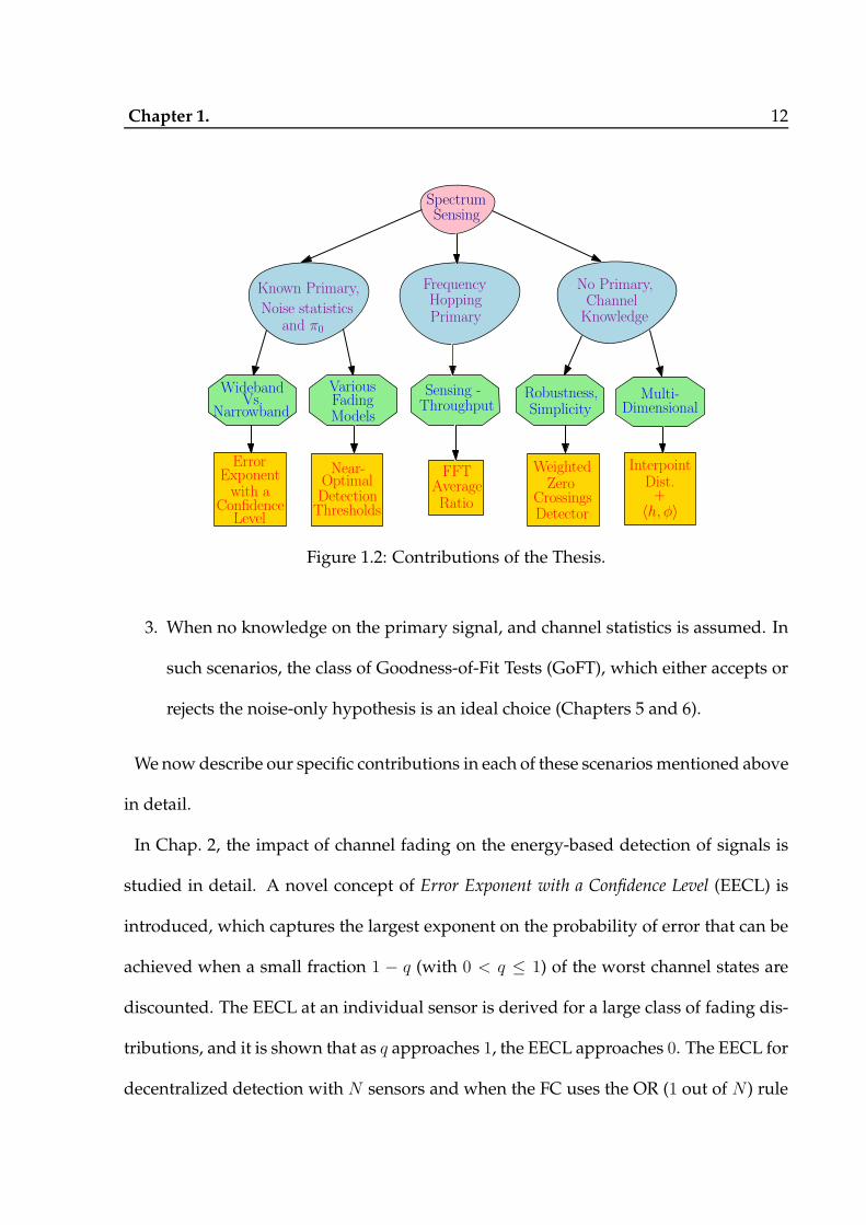
Chapter 1. 12

SpectrumSensing

FrequencyHoppingPrimary

No Primary,ChannelKnowledge

VariousFadingModels

Sensing -Throughput

Robustness,Simplicity

Multi-Dimensional

Near-

Thresholds

WeightedZero

CrossingsDetector

ErrorExponentwith a

ConfidenceLevel

FFTAverageRatio

InterpointDist.

〈h, φ〉+

Known Primary,

Noise statisticsand π0

Wideband

NarrowbandVs.

DetectionOptimal

Figure 1.2: Contributions of the Thesis.

3. When no knowledge on the primary signal, and channel statistics is assumed. In

such scenarios, the class of Goodness-of-Fit Tests (GoFT), which either accepts or

rejects the noise-only hypothesis is an ideal choice (Chapters 5 and 6).

We nowdescribe our specific contributions in each of these scenariosmentioned above

in detail.

In Chap. 2, the impact of channel fading on the energy-based detection of signals is

studied in detail. A novel concept of Error Exponent with a Confidence Level (EECL) is

introduced, which captures the largest exponent on the probability of error that can be

achieved when a small fraction 1 − q (with 0 < q ≤ 1) of the worst channel states are

discounted. The EECL at an individual sensor is derived for a large class of fading dis-

tributions, and it is shown that as q approaches 1, the EECL approaches 0. The EECL for

decentralized detection with N sensors and when the FC uses the OR (1 out of N) rule

Chapter 1. 13

is derived under the Rayleigh fading and lognormal shadowing channels. Closed-form

lower bounds on the EECL are also derived, for both Rayleigh fading and lognormal

shadowing channels. The bounds are easy to compute and become increasingly accu-

rate as q approaches 1. The theoretical development is used to successfully address the

question of NB versus WB sensing alluded to earlier (See Sec. 1.3.1), and a rigorous

analysis is presented. Specifically, if the ratio of normalized NB and WB powers ex-

ceeds a threshold, NB sensing is better than WB sensing in terms of the EECL, and vice

versa. The contents of this chapter has been published in part in [56].

Chapter 3 derives near-optimal thresholds for energy detection of signals under the

commonly used fading models, namely Rayleigh, lognormal, Nakagami-m, Weibull

and Suzuki distributions, for spectrum sensing under a Bayesian framework. For the

Rayleigh fading case, the trade-off between the number of observations and the pri-

mary power for given error performance is found. Extending the analysis to the decen-

tralized case, the error exponents at the Fusion Center (FC) as the number of sensors

grows large is derived. For the decentralized detection with Rayleigh fading, the diver-

sity gain on the overall probability of error is shown through simulations. The contents

of this chapter have been published in part in [57] and [58].

In Chap. 4, we apply an existing technique called the FFT Average Ratio (FAR) al-

gorithm for primary signal detection under a multiuser frequency-hopping primary

scenario, and derive closed-form expressions for the probabilities of false alarm and

detection as a function of the detection threshold, number of averaging frames, and

the estimated SNRs of the primary signal in the occupied bands. We define a utility

metric to quantify the throughput of the CR, and analytically obtain the CR sensing

Chapter 1. 14

duration that maximizes the throughput while satisfying a constraint on the maximum

allowable interference to the PUs. We implement the FARAlgorithm on a Lyrtech Small

Form Factor Software Defined RadioDevelopment Platform (Lyrtech SFF SDRDP), and

validate the implementation by comparing its performance with that obtained from the

analysis and simulations. The contents of this chapter have been published in [59].

In Chap. 5, we formulate the problem of spectrum sensing as a Goodness-of-Fit test,

and a detector based on the number of zero-crossings in the observations is proposed.

Given a target false alarm probability, near-optimal detection thresholds are obtained

for uniform and exponential weights. The proposed detector is shown to be robust

to two types of noise uncertainties encountered in practice, namely, noise parameter

uncertainty and the noise model uncertainty. In a detailed simulation study, the perfor-

mance of the proposed detectors is compared with existing techniques under various

primary signal models operating in different noise and fading environments. The con-

tents of this chapter have been published in [60].

Finally, in Chap. 6, we propose two GoFTs in a multi-dimensional setup where mul-

tiple observations recorded in a multi-sensor, multi-antenna environment are used by

the test. The proposed GoFTs are based on the properties of stochastic distances. The

advantages of the proposed detectors are highlighted, and the performance benefits

relative to existing techniques are illustrated through simulations. The contents of this

chapter have been published in [61].

List of Publications From This Thesis

Journal Papers

1. S. Gurugopinath, C. R.Murthy andV. Sharma, “Error exponent analysis of energy-

based bayesian decentralized spectrum sensing under fading,” submitted to IEEE

Transactions on Vehicular Technology.

2. S. Gurugopinath, R. Akula, C. R. Murthy, R. Prasanna and B. Amruthur, “Design

and Implementation of Spectrum Sensing for Cognitive Radios with a Frequency-

Hopping Primary System,” submitted to IEEE Transactions on Instrumentation

and Measurement.

3. S. Gurugopinath, C. R. Murthy and C. S. Seelamantula, “Zero-crossings based

spectrum sensing under noise uncertainties,” journal version under preparation.

Conference Papers

1. Sanjeev G., K. V. K. Chaythanya, and C. R. Murthy, “Bayesian decentralized spec-

trum sensing in cognitive radio networks,” Proc. International Conference on Sig-

nal Processing and Communications (SPCOM), Bangalore, India, Jul. 2010.

15

Chapter 1. 16

2. S. Gurugopinath, C. R.Murthy, andV. Sharma, “Error exponent analysis of energy-

based bayesian spectrum sensing under fading channels,” Proc. IEEEGlobal Telecom-

munications Conference (GLOBECOM), Houston, USA, Dec. 2011.

3. S. Gurugopinath, Raghavendra Akula, C. R. Murthy, R. Prasanna and B. Am-

ruthur, “Spectrum sensing with a frequency-hopping primary: from theory to

practice,” Proc. IEEE International Conference on Communications (ICC), Jun.

2014, Sydney, Australia.

4. S. Gurugopinath, C. R. Murthy and C. S. Seelamantula, ”Zero-crossings based

spectrum sensing under noise uncertainties,” Proc. National Conference on Com-

munications (NCC), Kanpur, India, Feb-Mar. 2014.

5. S. Gurugopinath, ”Near-optimal detection thresholds for bayesian spectrum sens-

ing under fading,” Proc. International Conference on Signal Processing and Com-

munications (SPCOM), Bangalore, India, Jul. 2014.

6. S. Gurugopinath, ”Multi-dimensional goodness-of-fit tests for spectrum sensing

based on stochastic distances,” Proc. International Conference on Signal Process-

ing and Communications (SPCOM), Bangalore, India, Jul. 2014.

Chapter 2

Error Exponent Analysis of

Energy-Based Bayesian Decentralized

Spectrum Sensing Under Fading

2.1 Introduction

Spectrum sensing, or the detection of the presence or absence of a primary signal in a

given frequency band of interest, is a well-studied topic in recent literature on Cognitive

Radios (CR) [1, 4]. Multi-sensor detection, or decentralized detection, is the preferred

approach for spectrum sensing, because of its resilience to signal fading, the hidden

node problem, etc. [10, 13, 31, 62–65]. In fixed sample-size decentralized detection, in-

dividual CR nodes make one-bit decisions about the availability of the spectrum using

a given number of samples, and the individual decisions are combined at a Fusion

Center (FC) to detect the presence or absence of the primary signal. Energy-based de-

tection, popularly referred to as Energy Detection (ED), is a well known technique for

spectrum sensing, wherein the signal energy in the band of interest is measured and

compared with a threshold [43, 46, 66, 67]. The primary signal is declared to be present

17

Chapter 2. 18

if the measured energy exceeds the threshold.

The detection probability performance of ED when the channel between the primary

transmitter and the secondary node undergoes narrowband Rayleigh fading has been

analyzed under the Neyman-Pearson (NP) framework [43, 66, 68]. Although closed-

form expressions for the probability of detection have been derived, due to the form of

the integrals involved, it is cumbersome to obtain the detection threshold that meets a

given minimum detection probability requirement. One way around this is to use an

alternative performance metric such as the error exponent [48, 49], which essentially

captures the asymptotic behavior of the probability of error performance of a detector

as the number of samples used for making decisions gets large.1 Mathematically, the

error exponent is defined as limM→∞− log(Pe)/M , where M is the number of samples

used for detection, and Pe is the corresponding probability of error. One of the early

studies on the error exponent performance of decentralized detection was the seminal

work of Tsitsiklis [45]. In the Bayesian framework, the exponent on the probability of

error of decentralized detection has been analyzed in [69]. The Bayesian error exponent

of mismatched likelihood ratio detectors was derived in [70]. The analysis uses the fact

that the best achievable exponent in the Bayesian probability of error is the Chernoff

information between the probability distribution functions under the two hypotheses.

In turn, this implies that the optimal exponents associated with the probability of false

alarm and the probability of missed detection must equal each other [48, Chap. 11], [71].

When the primary signal power or the noise variance at the secondary receiver are

unknown, a robust and blind detection scheme based on the maximum eigenvalue of

1The number of samples can be considered to be large, for example, in Digital Television (DTV) signaldetection, where the primary network changes its occupancy infrequently.

Chapter 2. 19

the sample covariance matrix has been proposed and studied through simulations [72].

In [73] and [74], multi-antenna assisted spectrum sensing is considered under the NP

framework.

Decentralized detection for spectrum sensing under the Bayesian framework is con-

sidered in [57, 75, 76]. Here, the channel between the primary transmitter and the

secondary sensors is assumed to undergo fading, while the channel between the sen-

sors and the FC is assumed to be lossless but finite-rate. However, to the best of our

knowledge, prior to this study, error exponents for energy-based decentralized spec-

trum sensing have not been derived in the literature. There are several advantages in

using the error exponent as a performance metric under a Bayesian set-up. First, the

optimal error exponent is independent of the specific values of the prior probabilities,

provided they are nonzero [48]. Due to this, the optimal error exponent, and detection

schemes based on maximizing the error exponent, are naturally robust to uncertain-

ties in estimating the prior probabilities, unlike detectors designed with the goal of

minimizing the probability of error. Further, error exponents allow one to contrast the

performance of competing detectors over a range of target performance requirements,

rather than at a single missed detection probability target. This is useful when choosing

between detectors at the design phase of a hardware implementation.

Yet another reason for considering an error exponent analysis of spectrum sensing

is related to the statistical properties of the fading experienced by the primary signal.

For Narrow-Band (NB) signals, the multipath (Rayleigh) fading effect is dominant, in a

non line-of-sight environment. On the other hand, Wide-Band (WB) signals spanmulti-

ple coherence bandwidths, due to which, the Rayleigh fading component averages out

Chapter 2. 20

when the signal energy is accumulated across the wideband, resulting in the lognormal

shadowing as the dominant fading component [47, 77]. As a concrete example, in the

IEEE 802.22 (WRAN) standard, the primary (Digital Television (DTV)) signal is a wide-

band signal, with a strong pilot tone at 2.69 MHz (see Figure 2.1).2 There are therefore

two options for detection. First, one could use an NB filter to capture just the pilot tone,

and detect based on the pilot energy. This has the advantage of filtering out the WB

noise; but the detector has to contend with a Rayleigh-faded NB signal. Alternatively,

one could use the energy in the entire WB signal for detection, which averages out the

Rayleigh fading [47,77], but the detector has to work against the lognormal shadowing

and the added impairment due to the AWGN over the WB. Again, due to the complex

form of the integrals involved, direct comparison of the two options using conventional

performance metrics such as the probability of error is difficult. Hence, in this chapter,

we contrast these two options by analyzing the Bayesian error exponent performance

of energy-based detection.

The main contributions of this work are as follows:

• The concept of Error Exponent with a Confidence Level (EECL) is introduced, which

captures the largest exponent on the probability of error that can be achieved if a

fraction 1 − q (with 0 < q ≤ 1) of the worst channel states are discounted. The

EECL at an individual sensor is derived for a large class of fading distributions,

and it is shown that as q approaches 1, the EECL approaches 0.

• The EECL for decentralized detection with N sensors and when the FC uses the

2Note that, at the time of writing this chapter, in the U.S., spectrum sensing is made optional in theIEEE 802.22 standard. However, in many countries other than the U.S. and European countries, reliabledatabases may not be available [78]. In these cases, spectrum sensing is essential.

Chapter 2. 21

0 2 4 6 8 10 1220

30

40

50

60

70

80

90

100

110

frequency (MHz)

PS

D (

dB

)

Figure 2.1: One sided PSD of IEEE 802.22 DTV wideband signal.

OR (1 out of N) rule is derived under the Rayleigh fading and lognormal shad-

owing channels.

• Closed-form lower bounds on the EECL are also derived, for both Rayleigh fading

and lognormal shadowing channels. The bounds are easy to compute and become

increasingly accurate as q approaches 1.

• The theoretical development is used to successfully address the question of NB

versus WB sensing, and a rigorous analysis is presented. Specifically, if the ratio

of normalized NB and WB powers exceeds a threshold, then NB sensing is better

than WB sensing in terms of the EECL, and vice versa.

We show, through Monte Carlo simulations, that our proposed detector outperforms

existing detectors in terms of the probability of error, when a small fraction of the worst

channel states are discounted. The improved sensing performance can lead to better

CR throughput and/or better primary user protection in CR implementations. Note

that, joint design of the sensing scheme and the medium access protocol to maximize

Chapter 2. 22

the secondary throughput [50, 79], while an important topic of study, requires one to

assume a specific model for the temporal behavior of the primary occupancy. Such a

study is beyond the scope of this chapter.

The rest of this chapter is organized as follows. The problem set-up and the basics of

error exponents are presented in Sec. 2.2. The EECL at a single node is introduced and

analyzed in Sec. 2.3. Distributed detection is considered in Sec. 2.4, where the EECL

at the FC with the OR rule is derived. The comparison between WB and NB spectrum

sensing in terms of the EECL is discussed in Sec. 2.5. Simulation results are presented

in Sec. 2.6, and Sec. 2.7 concludes the chapter. Proofs of the various theorems and

corollaries are presented in the Appendix.

2.2 SystemModel

We consider a decentralized detection set-up where N sensors use the average energy

measured from M independent observations each as the test statistic for making their

individual decisions between the signal absent (denoted H0) and signal present (de-

noted H1) hypotheses [10, 13, 31, 63, 64, 73, 80]. Such an energy-based test is known to

be optimal when no knowledge about the structure of the primary signal is available

at the CR nodes [46]. When M is large, using the Central Limit Theorem (CLT), the

test statistic can be well-approximated as being Gaussian distributed, resulting in the

following hypothesis test at each sensor [38, 66, 81]:

H0 : Vy ∼ N(0,

1

M

)

H1 : Vy ∼ EhN(|h|2 P, 1

M

), (2.1)

Chapter 2. 23

where Vy , 1M

∑Mk=1 |Yk|2 − 1 is the test statistic, and Yk is the kth observation at the

sensor. Also, N (µ, σ2) represents a normal distribution with mean µ and variance σ2.

In writing the above, without loss of generality, we normalize the receiver noise vari-

ance to unity. The average received power of the primary signal, P , is also assumed to

be known at the nodes. The noise variance and average received signal power can be

estimated, for example, using a calibration phase, when the primary signal is known

to be absent and present, respectively. Furthermore, for simplicity, we assume that the

CR nodes are sufficiently close to each other that P is the same at all nodes [76]. This

assumption is valid when the CR nodes involved in cooperative spectrum sensing are

located in proximity with each other, and are relatively far from the primary transmit-

ter. In such a situation, one can assume that the path loss from the primary transmitter

to the CR nodes, which is the main contributor to the average received power, is es-

sentially the same for all CR nodes.3 The expectation Eh in the above is taken over the

distribution over the channel gain, h, which is assumed to be random, unknown, and

constant for the M observations. In (2.1), we have omitted the sensor index from Vy

for notational convenience, since the observations are assumed to be independent and

identically distributed (i.i.d.) conditioned on the true hypothesis.

In the literature, various statistical models have been proposed for the channel h, de-

pending on the signal bandwidth and propagation environment. As mentioned earlier,

when the primary signal is NB, the Rayleigh fading component typically dominates the

3In practice, the average received power may not be the same at the sensors. However, one coulddesign the detectors assuming a certainminimum value of the average power at all sensors. If a particularsensor sees an average power larger than P , its detection probability will only be better than the designedvalue. Hence, this represents a conservative design approach in terms of protecting the primary users.

Chapter 2. 24

lognormal shadowing components, and hence |h|2 can bemodeled as exponentially dis-

tributed [82, 83]. When the primary signal is a WB signal, it spans multiple coherence

bandwidths, due to which, the Rayleigh fading components average out, resulting in

h being a lognormal shadowing random variable [47, 77]. Other models include the

Nakagami-m distribution, the Weibull distribution, and the Suzuki distribution [77].

In this work, we focus on the two most commonly used models, namely, the Rayleigh

and the lognormal shadowing distributions, for the NB and WB fading cases, respec-

tively. However, our main results can be extended to handle any of the fading models

mentioned above.

We assume that the sensors transmit their binary decisions to an FC through a finite

rate, noiseless, delay-free CR control channel, as in [75,76]. This simplifies the analysis,

and the corresponding EECL represents an upper bound on the error exponent achiev-

able in the general case. It is valid when the CRs use a low-rate dedicated control

channel to forward their decisions to the FC. The FC combines the individual decisions

using theK out ofN fusion rule to detect the presence or absence of the primary signal.

It is known that, when the individual sensor decisions are i.i.d. conditioned on the true

hypothesis, theK out ofN fusion rule is optimal in terms of probability of error [71,84].

In particular, we will focus on the 1 out of N fusion rule, i.e., the OR fusion rule, in the

sequel. We will show that the OR fusion rule has a certain optimality property in terms

of the error exponents. In the next section, we present the main results on the EECL at

an individual sensor. We extend it to multiple-node decentralized detection in Sec. 2.4.

Chapter 2. 25

2.3 Detection at the Sensors

We start by considering the single-sensor hypothesis testing problem in (2.1). The con-

ventional error exponent is defined as limM→∞− log peM

, where pe denotes the probability

of error at the sensor, and is given by π0pf + (1 − π0)pm, with π0, pf and pm denoting

the prior probability of hypothesis H0, the false alarm probability, and the missed de-

tection probability, respectively. Below, we show that the exponent on the probability

of missed detection is zero, provided the pdf of the channel gain is continuous and

satisfies P(|h|2 ≤ |h0|2) > 0 for arbitrarily small |h0| > 0, which is satisfied by all of

the distributions mentioned above. Therefore, the conventional error exponent analy-

sis is not useful for answering the question of NB vs. WB spectrum sensing. Essentially,

this happens because the deep fade instantiations, where the hypotheses are indistin-

guishable, dominate the average detection performance; and all detection techniques

perform equally poorly in this scenario. Hence, in this chapter, we propose the follow-

ing novel performance metric to evaluate and compare the performance of NB andWB

spectrum sensing approaches. The EECL at a single sensor is defined as given below.

We extend the definition to the N sensor case in the next section.

Definition 1. Let Sq denote a set of channel instantiations such that P(|h|2 ∈ Sq) = q. The

error exponent with a confidence level q, denoted EECL(q), is the maximum error exponent

achievable conditioned on |h|2 ∈ Sq, where the maximization is over all possible choices of Sq.

The above definition of the error exponent, discounting the deep fade instantiations,

Chapter 2. 26

has practical relevance. For example, in the IEEE 802.22 standard, the primary sig-

nal detection is required to achieve a probability of miss ≤ 0.1 with a sensing dura-

tion ≤ 2 seconds, whenever the primary signal power at the secondary node exceeds

−116 dBm [35]. Thus, typically, the primary network would require the CR to guaran-

tee a given probability of missed detection target whenever the signal power level at

the CR exceeds a given threshold. Now, in the single sensor case, it is immediate to see

that, among all possible choices for Sq, the highest error exponent is achieved by letting

Sq = |h|2 : |h|2 ≥ |h0|2, where the threshold |h0|2 depends on the minimum power

level at which the primary signal detection performance needs to be guaranteed by the

CR.

An alternative interpretation of the operational significance of the EECL is as follows.

Consider a given missed detection probability constraint, β, imposed by the primary

network. Pick 0 < α < β. For a fraction α of the channel states, the missed detection

probability can be upper bounded by unity. For the remaining fraction 1 − α of the

channel states, we set the detection threshold such that the missed detection probability

is at most β − α. Then, the overall missed detection probability is upper bounded by

β. As will be shown in the sequel, discounting a fraction α of the channel states allows

one to achieve a positive exponent on the probability of error. Hence, if one detection

scheme has a larger EECL than another, the detector with the larger EECL will have a

significantly smaller false alarm rate, and, consequently, better secondary throughput,

for the givenmissed detection probability constraint of β, as the number of observations

gets large. Hence, the EECL can be used as a metric for the design, and performance

comparison, of different detection schemes (e.g., NB vs. WB spectrum sensing).

Chapter 2. 27

The main result of this section is stated as the theorem below. It is valid as long as

the distribution of the gain of the channel from the primary transmitter to the sensors

is continuous and nonzero for infinitesimally small arguments. To obtain the result, we

use the fact that, under a Bayesian setup, the optimal exponent on the probability of er-

ror is achieved when the exponents on the probability of false alarm and the probability

of missed detection are equal [48, Chap. 11], [71].

Theorem 1. Let α , |h|2. The Bayesian hypothesis test defined in (2.1) achieves an EECL(q)

of (α0P )2

8, where α0 satisfies P (α ≥ α0) = q. Further, the optimal detection threshold on Vy

asymptotically approaches α0P2

asM gets large.

Proof. See Appendix A.1.

Under Rayleigh fading, fα(α) = e−α, α ≥ 0, and hence, P(α ≥ α0) = q leads to

e−α0 = q, or α0 = − log(q). Under lognormal shadowing, the cumulative distribution

function (cdf) of α is given by Fα(α) = 1 − Q((log(α)− µs)/σs), where Q(·) is the stan-

dard Gaussian tail function, and µs and σs are the shape and scale parameters of the

shadowing distribution, respectively. Hence, α0 = exp (σsQ−1(q) + µs). Also, note that

the both the error exponent and the detection threshold are independent of π0, the prior

probability of hypothesis H0, as expected ([48], Pg. 389). Therefore, the error exponent

is unaffected by uncertainties in the knowledge of π0. Conditioned on α > α0, each

individual sensor achieves an error exponent of (α0P )2/8 on pf and pm. An important

corollary to the above theorem is that when q = 1, under the commonly used fad-

ing models such as the Rayleigh, Rician, lognormal, Nakagami distributions, etc., only

α0 = 0 solvesP(α ≥ α0) = 1, and hence, the error exponent with q = 1 is zero. Thus, the

Chapter 2. 28

conventional error exponent cannot be used to choose between NB and WB sensing, as

both result in a zero error exponent.

Another useful aspect of the above theorem is the determination of the asymptoti-

cally optimal detection threshold at an individual sensor, α0P2. Due to its asymptotic

optimality, the local decision rule of comparing Vy toα0P2

will be assumed at all sensors

in the next section, where the EECL(q) performance at the FC with the OR fusion rule

is analyzed.

2.4 Detection at the Fusion Center

In this section, we consider an energy-based local decision rule at the individual sensors

with the threshold set as α0P2, where α0 is a parameter to be optimized. We consider the

OR rule for combining the individual decisions at the FC. We use the OR fusion rule

because it can detect the presence of the primary signal even if just one of the sensors

is not in a deep fade, and also because it possesses an optimality property that we will

show later in this section. The main result of this section is stated as the following

theorem.

Theorem 2. When the individual sensors employ energy detection and the FC employs the OR

fusion rule, the EECL(q), denoted ǫ(N)E , is given by ǫ(N)

E = (α0P )2

8, where α0 satisfies

P

N∑

j=1

(2αjα0

− 1

)2

I 2αjα0

>1 ≤ 1

= 1− q. (2.2)

In the above, αj is the random channel power gain from the primary transmitter to the jth sensor,

and IA is the indicator function, taking value 1 when the event A is true and 0 otherwise.


Chapter 2. 29

Note that the condition in (2.2) to determine α0 does not require the fading coefficients

from the primary transmitter to the individual sensors to be independent or identically

distributed. The joint distribution of the fading coefficients has to be used to evaluate

the probability in (2.2) to find the value of α0, and the solution cannot be obtained in

closed-form in the general case. When the fading coefficients are i.i.d., simpler equa-

tions that determine α0 for the cases of Rayleigh fading and lognormal shadowing are

stated as the corollary below.

Corollary 1. When the individual sensors employ energy detection with threshold α0P2

and

the FC employs the OR fusion rule, with i.i.d. Rayleigh fading channels between the primary

transmitter and the sensors, the EECL(q) is given by (α0P )2

8, where α0 satisfies

[1− exp

(−α0

2

)]N+

N∑

l=1

(N

l

)[1− exp

(−α0

2

)]N−lexp

(−α0

2l)P

l∑

k=1

a2k ≤ 1

= 1− q.

(2.3)

In (2.3), ak is exponentially distributed with parameter 2α0. The same detector, under i.i.d.

lognormal shadowing, with a threshold of ℓ0P2

at the individual sensors, achieves an EECL(q) of

(ℓ0P )2

8, where ℓ0 satisfies

PNA +

N∑

l=1

(N

l

)PN−lA P l

AcP

l∑

k=1

(eyk − 1)2 ≤ 1

= 1− q. (2.4)

In (2.4), yk has a truncated Gaussian distribution with mean µs + log(

2ℓ0

)and variance σ2

s ,

truncated to [0,∞). Also, PAc , Q

(−µs+log

(

2ℓ0

)

σs

), and PA , 1− PAc .


Note that both (2.3) and (2.4) need to be numerically solved to obtain α0 and ℓ0, respec-

tively. This, in turn, requires the probability terms in the expressions to be evaluated.

Chapter 2. 30

0 5 10 15 200

0.2

0.4

0.6

0.8

1

w

Cum

ula

tive

dis

trib

uti

on f

unct

ion F

(W)

W, with (0.9,0.165)

Corres. P−IV approx.

W, with (0.85,0.15)


W, with (0.5,0.165)


Figure 2.2: CDF of W ,∑10

k=1 (eyk − 1)2, where yk are i.i.d. and truncated Gaussian

distributed with (mean, variance) = (0.9, 0.165), (0.85, 0.15) and (0.5, 0.165), and yk > 0with probability 1.

To this end, we use the simple and tight approximation to the cdf of the sum of Weibull

random variates (with parameter c = 2) derived in [85] to evaluate the probability term

in (2.3) in closed-form. Also, we use the Pearson type IV distribution approximation

in [86] (see Fig. 2.2) to evaluate the probability term in (2.4), in closed-form. However,

we do not present the expressions here for the sake of brevity.

2.4.1 Extension to Unequal Average Received Signal Powers

Recall that, in the above, we had assumed that the CR nodes are sufficiently close to

each other that P is the same at all nodes. We now present an extension of our results to

handle unequal average received powers at the secondary nodes. First, we consider the

case of detection at individual sensors. If the average received power at the ith sensor is

Chapter 2. 31

Pi, the EECL(q) of that sensor is (α0Pi)2/8, where α0 is as defined in Theorem 1. Next,

for the detection at the fusion center, it is easy to see from the proof of Theorem 2 that

the exponent on the false alarm rate is (α0Pmin)2/8, where Pmin , min1≤i≤N Pi. The rest

of the proof of Theorem 2 also follows through, with P replaced by Pj in (A.7) and (A.8)

in Appendix A.2. Correspondingly, the condition on α0 in (2.2) gets modified as:

P

N∑

j=1

(PjPmin

)2(2αjα0

− 1

)2

I2αjα0

>1 ≤ 1

= 1− q. (2.5)

Note that, compared to (2.2), we have an extra (Pj/Pmin)2 factor in the summation, since

the average received powers are unequal. Hence, with the OR fusion rule, an error

exponent of ǫ(N)E = (α0Pmin)

2/8 is achievable, where α0 satisfies the condition in (2.5).

2.4.2 Lower Bounds on the EECL

In this subsection, we derive lower bounds on ǫ(N)E for NB andWB sensing. These lower

bounds are easy to calculate and become tight as q → 1. The values obtained from these

lower bounds can also be used as a good initialization for solving (2.3) and (2.4).

Corollary 2. In the set-up of Corollary 1, under i.i.d. Rayleigh fading channels, with a threshold

ofαLB0 P

2at the individual sensors, a lower bound on the EECL(q) is given by

(αLB0 P )2

8, where αLB0

satisfies

αLB0 = 2

(1− q

CN

) 1N

, with CN ,N∑

k=0

(N

k

)π

k2

Γ(1 + k

2

) 1

2k. (2.6)

Under i.i.d. lognormal shadowing, with a threshold ofℓLB0 P

2at the individual sensors, a lower

Chapter 2. 32

bound on the EECL(q) is given by(ℓLB

0 P )2

8, where ℓLB0 satisfies

ℓLB0 = 2 exp

−

√√√√2σ2s log

(1√2π

(C ′N

1− q

) 1N

) ,with C ′

N ,N∑

k=0

(N

k

)π

k2

(2σs)kΓ(1 + k

2

) .

(2.7)


2.4.3 Optimality of the OR rule

In this subsection, we show that the OR fusion rule satisfies a local optimality property.

We show that, when the detection threshold α0P2

at the individual sensors is chosen to

satisfy (2.2), the OR fusion rule minimizes the probability of error at the FC.

Theorem 3. For sufficiently large M, the OR fusion rule is probability of error optimal for

decentralized detection, when the individual sensors employ energy detection with threshold

α0P2.


2.5 Wideband Vs. Narrowband Spectrum Sensing

As discussed earlier, when the primary signal is a wideband signal containing a strong

pilot tone, spectrum sensing can either be carried out by collecting the signal energy

over its entire WB or over a small bandwidth around the pilot [47]. In this section,

we characterize the relative performance of these two schemes in terms of the EECL.

Let PNB and PWB denote the ratios of the energies of the NB and WB signals to their

bandwidths, respectively. Typically, PNB is significantly larger than PWB.

Chapter 2. 33

2.5.1 NB vs. WB Sensing at Individual Sensors

Let ǫNB and ǫWB represent the EECL(q) achieved under NB and WB spectrum sensing

at a single sensor, respectively. From Sec. 2.3, given q, setting α0 = − log q and ℓ0 =

exp(σsQ−1(q) + µs) ensures Pα > α0 = Pℓ > ℓ0 = q. Now, NB sensing outperforms

WB sensing in terms of EECL, i.e., ǫNB > ǫWB, whenever

(PNB

PWB

)2

>

(exp(σsQ

−1(q) + µs)

− log q

)2

. (2.8)

2.5.2 NB vs. WB Sensing at the Fusion Center

Similar to the above, let ǫ(N)NB and ǫ

(N)WB represent the EECL(q) achieved by the FC under

NB and WB spectrum sensing, respectively. For a given q, ǫ(N)NB > ǫ

(N)WB if (α0PNB)

2

8>

(ℓ0PWB)2

8, i.e., when

(PNB

PWB

)2

>

(ℓ0α0

)2

, (2.9)

where α0 and ℓ0 satisfy (2.3) and (2.4), respectively.

Note that we have used the Rayleigh fading and the lognormal shadowing assump-

tions only in evaluating the numerical values of α0 and ℓ0 above. That is, the above

procedure immediately extends to analyzing the EECL(q) of other fading distributions

such as Rician, Nakagami-m, Weibull, Suzuki, etc., and the framework can be used to

compare NB and WB sensing under various fading conditions.

Also note that, due to the difference in their bandwidths, the sampling rates under

NB and WB fading can be different. In the above, we considered the behavior of the

sensing performance with respect to M , the number of observations at each sensor.

However, the analysis can be easily extended to study the behavior with respect to the

Chapter 2. 34

sensing duration, as follows. Let fs,NB and fs,WB denote the sampling rates of the NB

and WB signals, respectively. Then, a given spectrum sensing duration of Tss leads to

a probability of error approximately given by PE,NB , exp(−Tssfs,NBǫNB) and PE,WB ,

exp(−Tssfs,WBǫWB) in the two cases. Suppose fs,WB = Bfs,NB, where B is the ratio of

bandwidths of the WB and NB signals. Thus, NB detection outperforms WB detection

in terms of the EECL with the same confidence q and when both detectors sense for the

same duration, if

(α0PNB)2

8> B

(ℓ0PWB)2

8. (2.10)

For a given signal bandwidth, as B is increased (i.e., as the bandwidth of the NB

signal is decreased), PNB also increases relative to PWB, since the NB filter captures the

energy in the pilot tone more accurately. If the NB signal consists of a pure pilot tone,

the ratio PNB

PWBincreases linearly with B. Thus, by using a large enough B, NB sensing

can be made to outperform WB sensing for a given sensing duration, since the factor

B appears quadratically in the error exponent term, while it occurs only linearly in

the detection delay term. However, increasing B comes at the cost of an increasing

accuracy in the CR’s knowledge of the frequency of the pilot tone in the primary signal.

2.6 Numerical Results and Simulations

In this section, we present simulation results to validate the analytical development in

the preceding sections, and to illustrate the relative performance of NB and WB sens-

ing schemes. For the NB and WB cases, we denote the signal powers by PNB and PWB,

Chapter 2. 35

and we let the channel gains be Rayleigh distributed and lognormal distributed, re-

spectively. The prior probability was chosen to be π0 = 0.5 for all the simulations.

For comparison with existing results, we extend the analysis in [66] to derive the prob-

ability of error with a confidence level, and then calculate the EECL(q) from it. We

also compare the performance of our detector with the detector designed under the

NP criterion [47], for both NB and WB cases, as well as for single sensor detection and

decentralized detection with multiple sensors.

2.6.1 Detection at the Sensors

In Fig. 2.3, we plot EECL(q) as a function of the confidence level q, for the NB and WB

fading models, with PNB

PWB= 3. In the WB fading case, we show the curves for three

typical values of the shadowing parameter σ2s . First, note that all the curves approach

an EECL of 0 as q approaches 1, i.e., the conventional error exponent is zero under

both NB and WB fading, as expected. As the confidence level is decreased, the NB

sensing outperforms the WB sensing. Also, in the single sensor case, the design in [66]

corresponds to using an NB detector. The excellent match between our results and

those derived from [66] is clear from the plot.

In order to show that it is possible to achieve a positive error exponent with a confi-

dence level under fading, we simulated the probability of error with confidence q = 0.9

at very low error probabilities, using importance sampling [87]. Figure 2.4 shows the

performance as a function of the average primary SNR, for various values of q. The

waterfall-type behavior of the curve indicates a positive error exponent. As mentioned

earlier, an advantage of the error exponent approach is that the threshold, τ = α0P2,

Chapter 2. 36

0.75 0.8 0.85 0.9 0.95 10

0.005

0.01

0.015

0.02

0.025

Confidence level q

Err

or

exponen

t ε e

NB, PNB

=1.5

NB, PNB

=1.5, using [67]

WB, σs

2 = 0.5625, P

WB=0.5

WB, σs

2 = 0.75, P

WB=0.5

WB, σs

2 = 1, P

WB=0.5

Figure 2.3: Trade-off between NB and WB sensing at a single sensor, with µs = 0 in theWB case.

is independent of the prior probability π0. In the figure, we see that the performance

with τ = α0P2

matches well with that obtained by using the near-optimal threshold de-

rived in [57]. We also illustrate the effect of mismatched π0 in Fig. 2.4. The performance

loss due to lack of knowledge of π0 is over 3 dB at a probability of error of 10−2, when

M = 106. For lower values ofM , the performance loss would be much higher, because

of the inverse square-root relationship between the number of samples and the SNR

required to achieve a given performance [57].

2.6.2 Detection at the Fusion Center

We now consider the decentralized set-up with the OR fusion rule for combining the

individual decisions from N sensors. In Fig. 2.5, we show the variation of the lower

bound on ǫ(N)E with confidence q = 0.99. The detection threshold parameters αLB0 and

Chapter 2. 37

−20 −15 −10 −5 010

−10

10−8

10−6

10−4

10−2

Average primary SNR (dB)

Pro

b.

of

erro

r w

ith

co

nfi

den

ce q

q=0.99

q=0.95

q=0.9

τ=α0P/2

Near−optimal τ

Mismatched τ

Figure 2.4: Variation of pe with a confidence q as a function of SNR, under narrowbandRayleigh fading. Here, N = 1, π0 = 0.5, M = 106. The curve labeled ’Mismatched τ ’corresponds to using π0 = 0.5 to design the detector, when the actual π0 = 0.01.

ℓLB0 are obtained from (2.6) and (2.7). We see that the lower bound closely approximates

the cross-over behavior of the NB and WB sensing schemes, shown in Fig. 2.6. For

obtaining the latter curve, the detection thresholds are found by numerically solving

(2.3) and (2.4) for the NB and WB cases, respectively.

We plot ǫ(N)E as a function of the power ratio PNB

PWBin Fig. 2.7, for different values of

q, and with N = 4. Both Figs. 2.6 and 2.7 show the cross-over between NB and WB

sensing: as PNB

PWBis increased, NB sensing outperforms WB sensing. Next, the variation

of ǫ(N)E with the number of sensors N is shown in Fig. 2.8, with the power ratio PNB

PWB= 1.

The plot shows an approximately linear improvement in the EECL(q) as the number of

sensors is increased.

Next, we present simulation results of the probability of error at the FC, PE , with

the signal modeled as the sum of a sinusoidal component and an AWGN component,

Chapter 2. 38

1 1.5 2 2.50

0.05

0.1

0.15

0.2

Power ratio PNB

/PWB

Low

er b

ound o

n e

rror

exponen

t ε E(N

)

NB, N=6

NB, N=4

NB, N=2

WB, N=6

WB, N=4

WB, N=2

Figure 2.5: Variation of the lower bound on ǫ(N)E as a function of PNB

PWB, with q = 0.99,

µs = 0, σs = 1.

varying ratio of their powers according to PNB

PWB. The bandwidths of the NB and WB

signals are fixed as 1 kHZ and 20 kHz, respectively. The sensing duration is chosen

as 20 ms. We compute the probability of error with confidence q by computing the

probability of error for 1000 i.i.d. channel states, and discounting a fraction 1 − q of

the channel states that yield the highest probability of miss when averaged over 10, 000

noise instantiations. Under this set-up, we plot the probability of error with N = 2, 4, 6

and confidence level q = 0.99 in Figs. 2.9 and 2.10. From Fig. 2.9, we see that the power

ratio at which the cross-over between NB and WB sensing occurs is roughly the same

as the cross-over points in the EECL plot of Fig. 2.6, i.e., the EECL does capture the

probability of error behavior of the detectors. In Fig. 2.10, we compare the performance

of our design with that of the NP-based design adopted in ([10, 47]), for both single-

sensor detection and decentralized detection, and for both the NB and WB cases. The

Chapter 2. 39

1 1.5 2 2.50

0.05

0.1

0.15

0.2

Power ratio PNB

/PWB

Err

or

exponen

t ε E(N

)

NB, N=6

NB, N=4

NB, N=2

WB, N=6

WB, N=4

WB, N=2

Figure 2.6: Variation of ǫ(N)E as a function of PNB

PWB, with q = 0.99, µs = 0, σs = 1.

NP test is designed to meet a false alarm probability target of 0.01. We see that, while

the probability of error with confidence q = 0.99 of the NP test saturates as the average

primary SNR increases, the performance of our EECL-based design exhibits a waterfall-

type drop with increasing SNR. Note that, for the settings in this simulation, the EECL

of NB sensing is higher than that of WB sensing. Since having a larger average primary

SNR is akin to having a larger number of observations at the individual sensors, one

would expect that NB sensing should outperform WB sensing as the average primary

SNR increases; this is also corroborated by Fig. 2.10.

Finally, Table 2.1 shows the values of α0 and ℓ0 for different q andN . It can be seen that

both α0 and ℓ0 increase with N and decrease with q. Using importance sampling, the

theoretical and experimental values of the error exponents obtained for different values

of P , q and N are listed in Tables 2.2 and 2.3. We note the good agreement between the

Chapter 2. 40

0.8 1 1.2 1.4 1.60

0.05

0.1

0.15

0.2

0.25

0.3

Power ratio PNB

/PWB

Err

or

exponen

t ε E(N

)

NB, q=0.9

NB, q=0.95

NB, q=0.99

WB, q=0.9

WB, q=0.95

WB, q=0.99

Figure 2.7: Variation of ǫ(N)E as a function of q, with N = 4, µs = 0, σs = 1.

theoretical and simulated error exponents, even at very low exponent values.

2.7 Conclusions

In this chapter, we analyzed the performance of energy-based Bayesian decentralized

detection for spectrum sensing in cognitive radios, with the exponent on the probabil-

ity of error as the performance metric. We showed that, for various fadingmodels, with

the OR rule for decision fusion, the error exponent is equal to zero. We introduced a

novel performance metric called the Error Exponent with a Confidence Level (EECL),

and showed that the EECL at a given confidence level q < 1 is strictly positive. We

used the EECL to answer the question of whether it is better to sense for the pilot tone

in a narrow band, or to sense the entire wide-band signal. We also derived simplified

Chapter 2. 41

2 4 6 8 100

0.1

0.2

0.3

0.4

0.5

0.6

0.7

0.8

Number of sensors

Err

or

exp

on

ent

ε E(N)

NB, q=0.9

NB, q=0.95

NB, q=0.99

WB, q=0.9

WB, q=0.95

WB, q=0.99

Figure 2.8: Variation of ǫ(N)E as a function of N , with PNB

PWB= 1, µs = 0, σs = 1.

expressions for finding the detection threshold and the EECL for the i.i.d. Rayleigh fad-

ing and lognormal shadowing cases. We validated the theoretical expressions through

simulations. Future work could include incorporating correlation in the signal or noise,

extending the results to allow for time-varying channels, and optimally combining NB

and WB spectrum sensing.

Chapter 2. 42

1 1.5 2 2.5 3 3.50

0.05

0.1

0.15

0.2

0.25

0.3

0.35

Power ratio PNB

/PWB

Pro

b.

of

erro

r w

ith

co

nfi

den

ce q

NB, N=6

NB, N=4

NB, N=2

WB, N=6

WB, N=4

WB, N=2

Figure 2.9: Variation of PE with a confidence level as a function of PNB

PWBwith q = 0.99,

µs = 0, σs = 1 and π0 = 0.5.

−20 −18 −16 −14 −12 −10 −8 −6 −4 −2

10−3

10−2

10−1

Average primary SNR (dB)

Pro

b.

of

erro

r w

ith

co

nfi

den

ce q

=0

.99

N=1, NB

N=4, NB

N=1, WB

N=4, WB

BayesianNeyman−Pearson

Figure 2.10: Comparison of the Bayesian and Neyman-Pearson approaches in termsof the PE with a confidence q = 0.99, as a function of the average primary SNR, withµs = 0, σs = 1 and π0 = 0.5.

Chapter 2. 43

Table 2.1: Values of α0 and ℓ0 for different q and N .

Nq = 0.9

Nq = 0.95

Nq = 0.99

α0 ℓ0 α0 ℓ0 α0 ℓ02 0.39 0.53 2 0.26 0.41 2 0.11 0.263 0.66 0.75 3 0.49 0.61 3 0.26 0.414 0.88 0.94 4 0.69 0.78 4 0.42 0.555 1.07 1.12 5 0.87 0.94 5 0.56 0.686 1.24 1.29 6 1.02 1.08 6 0.70 0.797 1.39 1.45 7 1.16 1.22 7 0.82 0.918 1.52 1.60 8 1.29 1.36 8 0.93 1.019 1.65 1.77 9 1.41 1.50 9 1.04 1.1210 1.76 1.92 10 1.52 1.63 10 1.14 1.23

Table 2.2: EECL(q) at a single sensor, with N = 1 and Rayleigh fading. All values haveto be multiplied by 10−5.

P (dB)q = 0.9

P (dB)q = 0.95

P (dB)q = 0.99

Th Sims Th Sims Th Sims−10 1.39 2.20 −2.25 11.84 14.28 0 1.26 2.32−7 5.55 6.57 −1.5 16.11 17.64 2 2.84 4.39−5 12.49 13.63 −1 21.05 22.30 3 5.05 7.34−4 22.02 23.56 −0.5 26.66 28.23 4 7.89 9.36−3 34.69 35.91 0 32.89 34.19 5 11.36 14.49

Table 2.3: EECL(q) at the FC, with P = −10 dB and Rayleigh fading. All values have tobe multiplied by 10−4.

Nq = 0.9

Nq = 0.95

Th Sims Th Sims2 1.94 2.11 2 0.87 0.883 5.41 6.12 3 2.97 3.524 9.73 10.28 4 5.93 6.34

Chapter 3

Near-Optimal Detection Thresholds for

Bayesian Spectrum Sensing

3.1 Introduction

As explained in Chapter 2, the under-utilization of the licensed radio spectrum, and

the consequent scarcity of bandwidth for newer wireless applications, can be allevi-

ated using cognitive radios. These are devices that can sense the radio spectrum and

transmit only when a primary user is not using a given band. Spectrum Sensing (SS),

or the problem of detecting the presence or absence of the primary transmissions, is

typically modeled as a problem of signal detection, where the goal is to test the hy-

pothesis H1 that the primary is on, against the hypothesis H0 that the primary is off.

The performance of the SS algorithm in CR systems at low primary SNR is of partic-

ular interest, since one has to ensure that the CR transmissions do not cause harmful

interference even at a primary receiver that receives a weak primary signal ([30,35,42]).

This needs to be ensured under the different possible fading environments that the CR

44

Chapter 3. 45

may encounter. A design based on a single fading model such as Rayleigh is neces-

sarily too restrictive. Hence, there is a need to develop detectors that offer guaranteed

performance under a variety of fading conditions.

Among the techniques proposed for SS, Energy Detection (ED) is one of the simplest,

from the point of view of implementability. The importance of the exploiting the fad-

ing model between the primary transmitter and CR using ED is well studied under the

Neyman-Pearson (NP) formulation. One of the earliest works on ED for NP for deter-

ministic signals was by Urkowitz [46], which was later extended in the context of SS

under various fading models by Digham et al. [43] and Zeng et al. [72]. Under a mix-

ture Nakagami distributed fading model (which has many well-known fading models

as special cases), the optimum detector, a locally optimum detector under low SNR

and a generalized likelihood ratio based detector have been studied in an NP context

by Astaneh and Gazor [88]. Conditions under which all the above mentioned detectors

perform better than ED are established. In all these works, the expressions of the PU

detection probability (pd), averaged over the channel distribution, for a given tolerance

level on the false-alarm (pf ) were derived. A comprehensive survey of algorithms for

ED under the NP formulation can be found in [30, 89].

Although the NP framework is commonly used in SS applications to design the test, it

suffers from the significant disadvantage of incorrectly assigning the null and alternate

hypothesis [90]. That is, it is more important, in the CR context, to find the threshold

that minimizes the pf for a given lower bound on pd, but most of the literature focuses

on maximizing pd under and upper bound constraint on pf . To overcome this issue, in

this chapter, we formulate the SS problem under a Bayesian setup, where the goal is to

Chapter 3. 46

minimize the probability of error. To the best of authors’ knowledge, a detailed study

of the performance of ED under various fading channel models in a Bayesian setup has

not been considered in the literature so far; the current chapter tries to fill this gap.

The primary challenge in Bayesian SS is to determine the detection threshold that

minimizes the probability of error. The optimal threshold depends on the fading model

between the primary transmitter and the CR node. In contrast, under the NP frame-

work, the detection threshold depends only on the signal statistics under the noise-only

hypothesis, not on the fading model. As mentioned in the previous chapter, the exact

analysis of the detection threshold, even for the simplest case of Rayleigh fading, is dif-

ficult. In this chapter, we are interested in deriving the near-optimal detection thresh-

olds for the Bayesian SS under various practical fading models such as Rayleigh [46],

lognormal [47], Nakagami-m [43], Weibull [91]. We are also interested in uncovering

the relationship between the number of samples used for detection, the detection SNR

and the average probability of error achieved. In this context, our main contributions

in this chapter are:

• We derive near-optimal detection thresholds for the commonly encountered fad-

ing models, viz., Rayleigh, lognormal, Nakagami-m, Weibull distributions, for

spectrum sensing under a Bayesian framework. The conditions under which each

approximation (near-optimality of the threshold) holds are highlighted.

• For the Rayleigh fading case, a fundamental relationship between the number of

observations and the primary SNR for achieving a given probability of error is

found.

Chapter 3. 47

• Extending the analysis to decentralized detection using ED at N sensors, the ex-

ponent on the probability of error at the Fusion Center (FC) is derived, as the

number of sensors grows large. This is different from the previous chapter, where

the error exponent was derived as the number of samples grows large, keeping

the number of sensors fixed.

• In the case of Rayleigh flat-fading primary signals, the diversity gain due to em-

ploying decentralized detection using multiple sensors is demonstrated using

Monte Carlo simulations. Also, an approximation for the Suzuki distribution [77]

is used to obtain an easily computable expression for the near-optimal detection

threshold under Suzuki fading.

The optimal thresholds derived in this chapter thus provide a comprehensive, near-

optimal solution set for Bayesian ED, under a variety of signal fading models that are

commonly encountered in CR applications.

The rest of the chapter is organized as follows. Section 3.2 explains the system model

considered in this work. Near-optimal detection threholds under various fading mod-

els are discussed in Sec. 3.3. In particular, the near-optimal detection thresholds for SS

under Rayleigh fading, lognormal shadowing, Nakagami-m fading, and Weibull fad-

ing are discussed in Secs. 3.3.1, 3.3.2, 3.3.3, and 3.3.4, respectively. The error exponent

at the fusion center under a general fading model between the primary transmitter and

individual sensors, and a lossless link between the sensors and the fusion center is de-

rived in Sec. B.4. Simulation results are discussed in Sec. 3.4, and the conclusions are

given in Sec. 3.5.

Chapter 3. 48

3.2 SystemModel

Consider a CR user which uses energy detection from M observations to carry out

spectrum sensing. At low SNR, and when M is reasonably large, using the Central

Limit Theorem (CLT) ( [38, 66, 81]), the statistic under both hypotheses can be modeled

as Gaussian distributed, leading to the hypothesis test

H0 : Vy ∼ N(0,

1

M

)

H1 : Vy ∼ EhN(|h|2 P, 1

M

), (3.1)

where Vy ,1

M

∑Mk=1 |Yk|2−1, with Yi representing the observations recorded by the CR

node. Without loss of generality, in writing the above, we have assumed that the noise

variance is unity. The notation Eh indicates the expectation operator over the random

channel h, which is assumed to be constant throughout the M observations. For the

problem in (3.1), the likelihood ratio (LR) is given by

LR(Vy) =

∫∞0

exp[− (Vy−αP )2

2/M

]fα(α)dα

exp[− V 2

y

2/M

] , (3.2)

where α , |h|2 represents the random channel gain. For the commonly encountered

channel fading models for |h| such as Rayleigh, lognormal, Nakagami-m, and Weibull,

the channel gain |h|2 is distributed as exponential, lognormal, gamma and Weibull,

respectively. Additionally, |h|2 can also be modeled as the Suzuki distribution, to con-

sider the effect of both small scale and large scale fading (Rayleigh and lognormal,

respectively). From elementary detection theory, it is known that the optimal test (that

minimizes the probability of error) for the hypothesis test in (3.1) is a test on LR(Vy),

Chapter 3. 49

which is of the form

LR(Vy)H0

≷H1

π01− π0

, (3.3)

where π0 is the prior probability of H0, assumed to be known. In the next section, we

show that, under fairly general conditions on the fading distribution fα(α) the above

test reduces to a test on Vy, i.e., to a test of the following form

VyH0

≷H1

τ(π0,M, P, ph), (3.4)

where τ(π0,M, P, ph) is the optimal detection threshold, and is a function of parame-

ters π0,M , P and on the set of parameters of the fading distribution considered (which

is denoted by ph). We also show the conditions under which the test on Vy in (3.4) is

optimal for a particular fading model. By a simple substitution, it can be easily shown

that when the test is of the form (3.4), the probabilities of false-alarm, missed detection

and overall error are given by

pf , PVy > τ(π0,M, P, ph)|H0=Q(τ(π0,M, P, ph)

√M), (3.5)

pm , PVy ≤ τ(π0,M, P, ph)|H1=∫ ∞

0

Q(−√M(τ(π0,M, P, ph)−αP )

)fα(α)dα,

(3.6)

pe = π0 pf + (1− π0) pm, (3.7)

where Q(·) represents the Gaussian Q-function.

Chapter 3. 50

3.3 Detection Under Various Fading Models

3.3.1 Detection Under Rayleigh Fading

When the channel |h| is Rayleigh distributed, |h|2 follows the standard exponential dis-

tribution. The following theorem gives an approximate solution to the threshold that

minimizes the probability of error for the hypothesis testing problem in (3.1).

Theorem 4. When the channel between primary transmitter and the CR node is Rayleigh

distributed, the detector for the problem considered in (3.1) has an approximate critical region

given by

Vy ≥ x(R)CLT , 1

MP+ 1√

M

√2 log

(1 +

(π0

1−π0

)P√2πM

). (3.8)

Proof. See Appendix B.1

The above result allows one to determine how M needs to scale with the received

average primary power P to obtain a given pe, which is stated as the corollary below.

Corollary 3. The probability of error for the hypothesis testing problem in (3.1) under the

Rayleigh fading case (given in (B.1)) depends on P andM only through the product P√M .

The above corollary follows directly by substituting the optimum threshold x(R)CLT in

(3.8) into (3.7), and verifying that pe depends only upon the product P√M . The utility

of the corollary is that it shows, for example, that if average received primary signal

power reduces by 3 dB, the probability of error performance can be retained by increas-

ing the number of observations by a factor of four.

Chapter 3. 51

3.3.2 Detection Under Lognormal Shadowing

In wideband SS (for instance, in the first DTV 802.22 proposed standard), the primary

signal spans multiple coherence bandwidths, due to which, the small scale (for e.g.,

Rayleigh) fading components average out ( [47], [77]). Under this model, the channel

gain ℓ , |h|2 is modeled as lognormal distributed with parameters µs and σ2s . That is,

ℓ = eµs+σsS, where S is a zero mean, unit variance Gaussian distributed random vari-

able. The following theorem gives an approximate solution to the near-optimal thresh-

old, under lognormal shadowing. Before stating the theorem, we present a heuristic

observation based on extensive simulations, which gives the conditions under which a

lognormal distribution can be well approximated by a Gaussian distribution.

Result 1. When the parameter σ2s is small and around zero,then, for the purpose of designing

detection thresholds, the distribution of a lognormal random variable with parameters µs and σs

can be approximated by a Gaussian distribution with mean eµs and variance e2µsσ2s , i.e.,

LN (µs, σs)d.≈ N (eµs , e2µsσ2

s). (3.9)

The intuition behind the above observation is as follows. Let X ∼ LN (µs, σs). When

the value of σs is low, defining x = eµs(1 + ǫ), we have

P(X ≤ x) = 1−Q

(log |x| − µs

σs

)≈ 1−Q

(µs + log(1 + ǫ)− µs

σs

)≈ 1−Q

(ǫ

σs

)(3.10)

when ǫ is a small positive real number. Approximating the PDF ofX asX ∼N (eµs , e2µsσ2s)

gives:

P(X ≤ x) = 1−Q

(x− eµs

eµsσs

)≈ 1−Q

(eµs(1 + ǫ)− eµs

eµsσs

)= 1−Q

(ǫ

σs

). (3.11)

Chapter 3. 52

Therefore, for small values of ǫ (which will be the case of interest for the SS problem

when σs is small), (3.11) and (3.10) are equal. The accuracy of the approximation is

highlighted in Figs. 3.1 and 3.2.

1 1.5 2 2.5 3 3.5 4

10−4

10−3

10−2

10−1

100

x

Cum

ula

tive

dis

trib

uti

on f

unct

ion F

L(x

)

Lognormal σ=0.01

Corres. Normal appx.

Lognormal σ=0.05


Lognormal σ=0.1


Figure 3.1: CDF of Lognormal distribution for various values of its log-shape parame-ter, and the corresponding Normal CDF approximation.

Theorem 5. When the channel between primary transmitter and the CR node follows a lognor-

mal distribution, the Bayesian detection problem considered in (3.1) has an approximate critical

region given by

Vy : Vy ≥ x

(WB)CLT ,

1

M

[√2

(M +

1

P 2σ2s

)(log

(π0

1− π0+Kc

)−logKc

)− 1

Pσ2s

]

(3.12)

where,

Kc ,exp

(− 1

2σ2s

)

√1 +MP 2σ2

s

. (3.13)

Chapter 3. 53

0 0.5 1 1.5 2 2.5 3

10−4

10−3

10−2

10−1

100

x

Com

ple

men

tary

CD

F 1

−F

L(x

)

Lognormal σ=0.01


Lognormal σ=0.05


Lognormal σ=0.1


Figure 3.2: CCDF of Lognormal distribution for various values of its log-shape param-eter, and the corresponding Normal CCDF approximation.

Proof. See Appendix B.2.

3.3.3 Detection Under Nakagami-m Fading

Note that, in the Bayesian hypothesis testing problem in (3.1), if |h| follows a Nakagami-

m distribution [77] with a positive integer parameterK, then g , |h|2 follows a gamma

distribution, with PDF fG(g) =gK−1e−g

Γ(K). The following theorem gives the near-optimal

detection threshold under Nakagami-m fading.

Theorem 6. Let the channel between primary transmitter and the CR node be Nakagami-m

distributed. For the Bayesian hypothesis testing problem considered in (3.1), the optimal test is

of the form (3.4), i.e., ED is optimal. Further, the solution to the following equation yields the

Chapter 3. 54

near-optimal detection threshold x(Nm)CLT :

KK

PKΓ(K)exp

(x(Nm)CLT − K

MP

)2

2/M

(

1

M

)K−12

[[i√2 sign

(x(Nm)CLT − K

MP

)]K−1√

2π

M

Γ(1/2)

Γ(1− K

2

) + (K − 1)Γ(1/2)

Γ(1− K

2

) ×

(x(Nm)CLT − K

MP

)2

2/M− i

Γ(−1/2)

Γ(−K−1

2

) ×

(x(Nm)CLT − K

MP

)

√2/M

−[(

x(Nm)CLT − K

MP

)K−1

Q

(−x

(Nm)CLT − K

MP√1/M

)]]− π0

1− π0= 0, (3.14)

provided the solution is close to the value KMP

. Here, i ,√−1. Otherwise, ED may not be

optimal.

Proof. See Appendix B.3.

Although (3.14) cannot be solved in closed-form, numerically solving it to obtain the

threshold x(Nm)CLT is not difficult. Theorem 6 shows that ED is optimal when x

(Nm)CLT is close

to KMP

. Following this, a simple, suboptimal detector can be proposed as follows (this

can be used in the Rayleigh fading case also, by setting K = 1), which compares Vy to a

threshold xsubCLT:

VyH1

≷H0

xsubCLT ,K

MP. (3.15)

We will illustrate the performance of the above suboptimal detector via Monte Carlo

simulations in Sec. 3.4.

3.3.4 Detection Under Weibull Fading

Weibull fading model is typically used to model the attenuation due to fading in wire-

less applications operating in 800-900 MHz range ( [92], [91], [77]). In this case, the

Chapter 3. 55

channel |h| is Weibull distributed, and W , |h|2 is also a Weibull distributed ran-

dom variable. If W(aw, bw) denotes a Weibull distributed variable with shape and

scale parameters aw and bw respectively, it is known that when |h| ∼ W(aw, bw), then

|h|n ∼ W(awn, bnw), for any positive integer n. Therefore, the PDF ofW is given by

fW (w; aw; bw) =aw2b2w

(w

b2w

)aw2

−1

exp

(−(w

b2w

)aw2

), w ≥ 0. (3.16)

The resulting integral in the numerator of (3.2) is hard to obtain in closed form. Hence,

we use a normal approximation on Weibull distribution ( [93], [94]), which, as seen in

Figs. 3.3 and 3.4, gives a good fit for large values of the shape parameter aw. Restriction

of the analysis for larger values of aw is in agreement with a result that for fading in

wireless communications around 900MHz, Weibull fit with larger values of the shape

parameter aw is sufficiently accurate [95]. The mean and the variance of the approxi-

mated normal random variable are given by

µw , bwΓ

(1 +

1

aw

)

σ2w , b2w

[Γ

(1 +

2

aw

)− Γ2

(1 +

1

aw

)]. (3.17)

Theorem 7. When the channel between primary transmitter and the CR node follows aWeibull

distribution, the Bayesian detection problem in (3.1) has an approximate critical region

Vy : Vy ≥ x

(W )CLT ,

1

M

[√2

(M +

1

P 2σ2w

)(log

(π0

1− π0+Kw

)−logKw

)− µwPσ2

w

](3.18)

Chapter 3. 56

0.5 1 1.5 210

−4

10−3

10−2

10−1

100

w

Cum

ula

tive

dis

trib

uti

on f

unct

ionF

W(w

)

Weibull bw

=1 aw

=4

Corres. Normal appx.Weibull b

w=1 a

w=6


w=1 a

w=8


Figure 3.3: CDF of the Weibull distribution for various values of its scale and shapeparameters, and the corresponding Normal CDF approximation.

where

Kw ,exp

(− µ2w

2σ2w

)

√1 +MP 2σ2

w

. (3.19)

Proof. The proof is similar to the proof of Theorem 5, and follows by using the approx-

imation given in (3.17).

In Sec. B.5, we discuss detection under Suzuki distribution [77]. Unfortunately, the

analysis of the optimal detection threshold is very hard for the case of Suzuki distri-

bution, because of its complicated integral form. In order to simplify the probabil-

ity of detection expressions, we approximate the Suzuki distributed random variable

with a generalized Gamma distribution [96]. However, the evaluation of LR(Vy) is not

Chapter 3. 57

0 0.5 1 1.510

−4

10−3

10−2

10−1

100

w

Com

ple

men

tary

CD

F 1

−F

W(w

)

Weibull bw

=1 aw

=4


w=1 a

w=6


w=1 a

w=8


Figure 3.4: CCDF of the Weibull distribution for various values of its scale and shapeparameters, and the corresponding Normal CCDF approximation.

straightforward even after this approximation, and hence, the optimal detection thresh-

old has to be evaluated through numerical techniques.

In Appendix B.4, we consider a decentralized setup and derive the error exponent

on the probability of error at a Fusion Center (FC), as a function of pf and pm at the

individual sensors. With some algebra, it can be shown that the right hand side of (B.22)

is strictly positive. A diversity-like improvement in PE is obtained with increasing N ,

and further insights can be drawn from the simulation results, discussed in Sec. 3.4.

3.4 Simulation Results

Our simulation setup consists of N sensors, usingM observations each, with a average

primary SNR observed at each sensor denoted by P . The range of P and a target PE

is typically specified by the primary network. This, in turn, dictates the value of M

Chapter 3. 58

103

104

1.02

1.04

1.06

1.08

1.1

1.12

Number of observations M

Opti

mal

thre

shold

xC

LT

(R)

P=1, Opt.

P=1, CLT

Figure 3.5: Variation of x(R)CLT withM for the optimum and CLT schemes.

and the detection threshold, such that the resulting PE is within the target specified by

the primary network. For all plots, π0 was fixed to be 0.5. First, consider the case with

N = 1. Figure 3.5 shows the comparison of the optimum threshold (curve labeled Opt.,

obtained through simulations by sweeping over a range of thresholds) with that of the

near-optimal threshold for the Rayleigh fading case (curve labeled CLT), indicating that

the x(R)CLT given in (3.8) is a good approximation. As expected, when M increases, x

(R)CLT

goes close to zero.

Figure 3.6 plots the probability of error pe versus average primary SNR P to show that

keeping P√M constant as P varies maintains a fixed probability of error level at the

detector. In this example, M was chosen as 500 for P = 1 and (P,M) are varied such

that P√M is constant. The two additional curves show the performance for a constant

M (chosen as 222, and 2000, corresponding to the value ofM needed to obtain the pe at

Chapter 3. 59

0.5 1 1.5

10−1

Primary SNR

Pro

bab

ilit

y o

f er

ror

Const. M1/2

P

M = 222

M = 2000

Figure 3.6: A constant pe can be maintained if P√M remains fixed.

the two extreme values of P ).

Figures 3.7 and 3.8 show the variation of the optimal threshold for the shadowing

case (σdB = 0.5) and weibull fading case (aw = 5, bw = 1), respectively, as a function

of M , for various values of P . As expected, the approximations become tighter for

high M and low P . A similar trend is seen in Fig. 3.9, where the simulated value

of optimal threshold for the Nakagami-m fading case with K = 10 is compared with

the corresponding theoretical near-optimal threshold derived in (3.14), as a function

of M , for various values of P . Also, the value of suboptimal threshold indicated in

(3.15) is plotted. It is observed that for the Nakagami-m case, the regime of number

of observations where our derived results hold is seen to be about ten-fold higher (∼

105) as compared with the corresponding regimes in the case of lognormal or Weibull

fading (∼ 104), to achieve the same probability of error.

Chapter 3. 60

Now, consider the decentralized detection case withN > 1. In Fig. 3.10, the quantities

− logPE

Nand the theoretical ǫE is plotted as a function of the number of sensors N for

M = 5, 80, and P = 0.1dB,−5.9dB, respectively. As N becomes large, the quantity

− logPE

Napproaches the theoretical exponent given in (B.22). For both values of P , the

values of M are chosen such that P√M is a constant. Therefore, the simulated curves

corresponding to − logPE

Nare nearly equal, as expected from Corollary 3. Figure 3.11

plots the PE at the FC vs. the average primary SNR P , using N = 1, 3 sensors, which

illustrates the diversity advantage that can be obtained by multi-sensor decentralized

detection. The optimum detection threshold andKopt was obtained from simulations.

0.5 1 1.5 2

x 104

0.02

0.025

0.03

0.035

0.04

0.045

0.05

0.055

0.06

0.065

Number of Observations

Opti

mum

Thre

shold

Sim., P=−9dB

Sim., P=−10dB

Sim., P=−11dB

Sim., P=−13dB

Th., P=−9dB

Th., P=−10dB

Th., P=−11dB

Th., P=−13dB

Figure 3.7: Simulated optimal thresholds and near-optimal theoretical thresholds forthe shadowing fading case, with its log-scale parameter σdB = 0.5.

Chapter 3. 61

0.5 1 1.5 2

x 104

0.02

0.025

0.03

0.035

0.04

0.045

0.05

0.055

0.06


Opti

mum

Thre

shold

Sim., P=−9dB

Sim., P=−10dB

Sim., P=−11dB

Sim., P=−13dB

Th., P=−9dB

Th., P=−10dB

Th., P=−11dB

Th., P=−13dB

Figure 3.8: Simulated optimal thresholds and near-optimal theoretical thresholds forthe Weibull fading case, with aw = 5, bw = 1.

3.5 Conclusions

This chapter considered the problem of Bayesian decentralized SS in CR networks un-

der various fading environments. A CLT-based approximation to the problem was

explored, which lead to analytically tractable expressions for near-optimal detection

thresholds that minimize the probability of error under Rayleigh, Lognormal, Nakagami-

m, Weibull fading cases. For the Suzuki fading case, a generalized gamma approxima-

tion was provided, which saves on the computation of an integral. Also, in the Rayleigh

fading case, it was shown that the probability of error at the individual sensors, in the

low SNR regime, is a function of P√M , where P is the received primary power and

M is the number of observations needed for detection. Extending to the decentralized

Chapter 3. 62

0.5 1 1.5 2

x 105

10−6

10−5

10−4

10−3

10−2


Opti

mal

Thre

shold

Sim., P=−13dB

Sim., P=−4dB

Sim., P=−1dB

Near−opt., P=−13dB



Sub−opt., P=−13dB



Figure 3.9: Simulated optimal thresholds and near-optimal theoretical thresholds forthe Nakagami-m fading case, with K = 10.

case with N sensors, the optimal exponent on the probability of error at the FC was de-

rived in closed form. The accuracy of the theoretical expressions and the diversity gain

obtainable through the use of multiple sensors were illustrated through simulations.

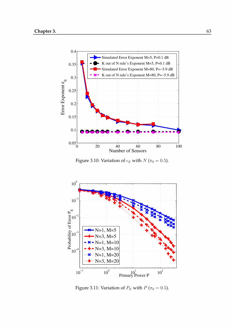
Chapter 3. 63

0 20 40 60 80 1000.05

0.1

0.15

0.2

0.25

0.3

0.35

0.4

Number of Sensors

Err

or

Exponen

t ε E

Simulated Error Exponent M=5, P=0.1 dB

K out of N rule’s Exponent M=5, P=0.1 dB

Simulated Error Exponent M=80, P=−5.9 dB

K out of N rule’s Exponent M=80, P=−5.9 dB

Figure 3.10: Variation of ǫE with N (π0 = 0.5).

10−1

100

101

102

10−4

10−3

10−2

10−1

100

Primary Power P

Pro

bab

ilit

y o

f E

rro

r P

E

N=1, M=5

N=3, M=5

N=1, M=10

N=3, M=10

N=1, M=20

N=3, M=20

Figure 3.11: Variation of PE with P (π0 = 0.5).

Chapter 4

Design and Implementation of

Spectrum Sensing with a

Frequency-Hopping Primary System

4.1 Introduction

A Cognitive Radio (CR) [1] operates by sensing the spectrum for Primary User (PU) ac-

tivity, and transmitting only in those frequency bands where the PU signal is observed

to be absent. The detection of PU activity is accomplished via Spectrum Sensing (SS),

which is the binary hypothesis testing problem of detecting the presence or absence of

a PU in the frequency-band of interest. In Chapter 2, we presented a detailed survey of

recent literature on SS.

It is clear that, in order to maximize the CR’s throughput while offering adequate

protection to the primary, it is important to tune the various sensing and CR trans-

mission related parameters such as the sensing duration, threshold, transmit power,

etc., considering the primary signal characteristics. The problem of SS is particularly

challenging when the primary users employ Frequency Hopping (FH) signaling, since

64

Chapter 4. 65

the CR needs to detect and exploit the available frequency bins within the short hop

duration of the primary.

The focus of this chapter is on the detection of FH primary signals. FH signals are typi-

cally used in secure/military applications and in standards such as IEEE 802.15.1/Blue-

tooth. SS of FH primary signals is challenging due to the frequently changing na-

ture of the primary frequency band [97], and has received relatively less attention in

the CR literature. Some early work on the detection of frequency-hopped signals in-

clude [98–100]. In these studies, the received signal is passed through a bank of Band

Pass Filters (BPFs), and a decision on the signal presence in each frequency bin is made

from the energy computed in each BPF, in time domain. Also, implementations of

spectrum sensing in a non-FH primary environment have been demonstrated using

off-the-shelf hardware platforms in [101–103].

To the best of our knowledge, however, past work on detecting FH signals has fo-

cussed primarily on detecting the presence or absence of an FH primary signal itself,

not on detecting unoccupied bands within each hop duration. Detecting and exploiting

unoccupied bands within the wider bandwidth over which primary users execute their

hopping patterns can lead to the harvesting of significant RF spectrum for CR com-

munications. To this end, in this chapter, we consider energy-based detection of unoc-

cupied bands in the presence of FH primary signals, and evaluate its efficacy through

rigorous theoretical analysis, Monte Carlo simulations, and implementation on a hard-

ware platform.

In this chapter, we study performance of the Fast Fourier Transform (FFT) Averaging

Ratio (FAR) algorithm [101,104], an energy-based detection scheme, for the problem of

Chapter 4. 66

sensing FH signals in CR applications. We consider the FAR algorithm for detection be-

cause of its computational simplicity and ease of implementation in a software defined

radio environment. Our novel contributions are as follows:

• We extend the FAR algorithm to the multiuser FH-PU scenario, and derive closed-

form expressions for the probabilities of false alarm and detection, as a function

of the detection threshold, number of averaging frames, and the estimated SNRs

of the primary signal in the occupied bands (Sec. 4.3.1).

• We define a utility metric to quantify the throughput of the CR, and obtain the CR

sensing duration that maximizes the throughput while satisfying a constraint on

the maximum allowable interference to the PUs (Sec. 4.3.2).

• We implement the FAR Algorithm on a Lyrtech Small Form Factor Software De-

fined Radio Development Platform (Lyrtech SFF SDR DP), and validate the im-

plementation by comparing its performance with that obtained from the analysis

and simulations (Appendix C.3 and Sec. 4.4).

Allowing for implementation losses, we show that the results obtained from the hard-

ware corroborate well with those obtained through theory as well as Monte Carlo sim-

ulations. We conclude, therefore, that the FAR algorithm is an easy-to-implement and

effective solution to the SS problem with an FH-PU network.

The rest of the chapter is organized as follows. The system model, and the FAR algo-

rithm are given in Sec. 4.2. The associated probabilities of false-alarm and detection of

the FAR algorithm as applied to SS with FH primary signals are derived in Sec. 4.3.1,

and the optimum sensing duration that maximizes the CR throughput is derived in

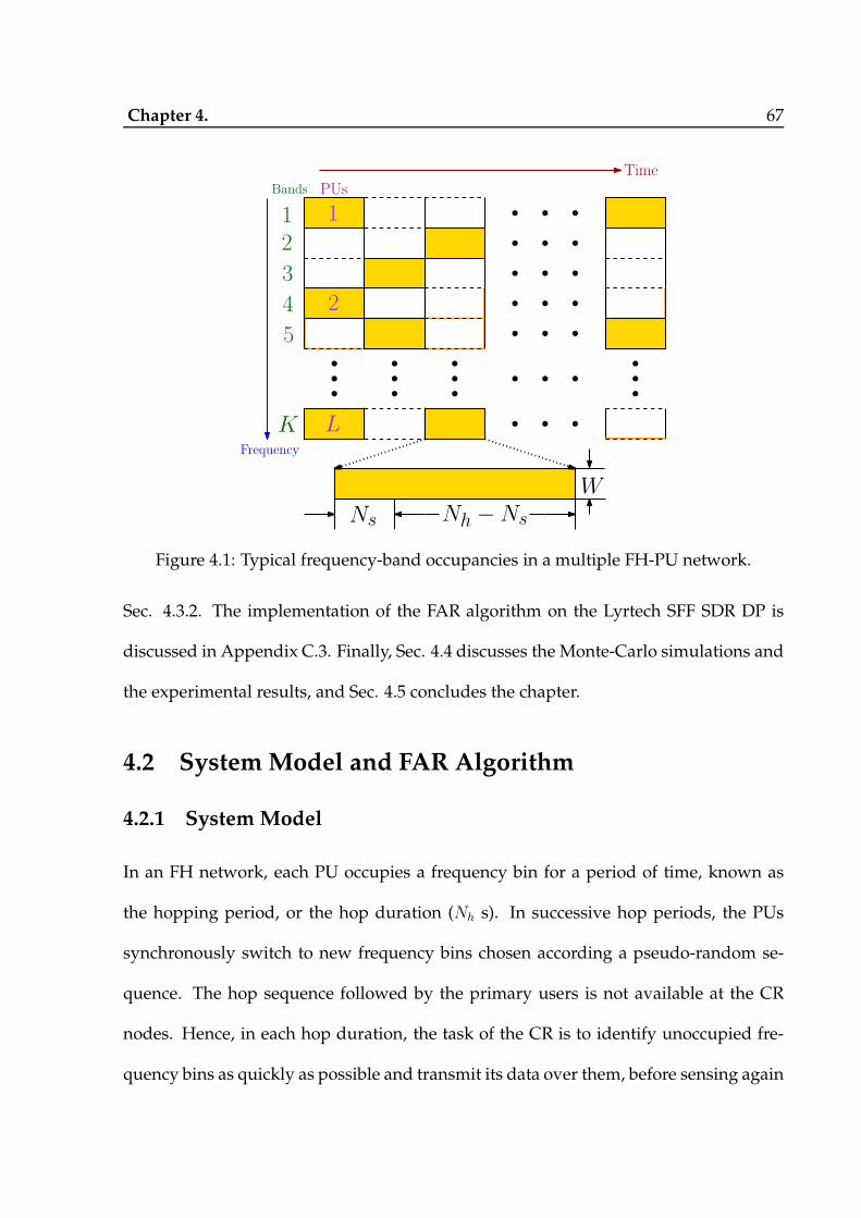
Chapter 4. 67

Ns Nh −Ns

Frequency

Time

1

2

L

1

2

3

4

5

K

Bands

W

PUs

Figure 4.1: Typical frequency-band occupancies in a multiple FH-PU network.

Sec. 4.3.2. The implementation of the FAR algorithm on the Lyrtech SFF SDR DP is

discussed in Appendix C.3. Finally, Sec. 4.4 discusses the Monte-Carlo simulations and

the experimental results, and Sec. 4.5 concludes the chapter.

4.2 SystemModel and FAR Algorithm

4.2.1 System Model

In an FH network, each PU occupies a frequency bin for a period of time, known as

the hopping period, or the hop duration (Nh s). In successive hop periods, the PUs

synchronously switch to new frequency bins chosen according a pseudo-random se-

quence. The hop sequence followed by the primary users is not available at the CR

nodes. Hence, in each hop duration, the task of the CR is to identify unoccupied fre-

quency bins as quickly as possible and transmit its data over them, before sensing again

Chapter 4. 68

during the next hop period of the primary network.

Suppose the CR wishes to find a spectrum hole of bandwidth W Hz within a wider

band of interest of bandwidth B Hz. Let B = KW i.e., the bandwidth B consists of

K contiguous, non-overlapping bins. We assume that, at any given hop duration, each

active primary user occupies one of the K bins, as shown in Fig. 4.1. The shaded bins

in Fig. 4.1 represent the bins occupied by the PUs at some given hop interval; there are

L active PUs in the figure. The primary signal hopping pattern is modeled as an i.i.d.

random sequence both across users and across time, and uniformly distributed over

the K bins. The CR down-converts the received signal, band-limits it to B Hz, and

samples it at a rate of fs ≥ 2B samples/s. In this chapter, for simplicity, we assume

that the number of active PUs, denoted by L, is known. In practice, since the number of

active PUs typically varies very slowly compared to the bin occupancy patterns, it can

be estimated and tracked based on the sensing outcomes. Let u ∈ 0, 1K represent the

primary occupancy pattern, where u(k) takes the value 0 or 1, depending on whether

the kth frequency band is free or occupied, respectively.

The CR collects Ns = N M data samples, groups them into M frames of N samples

each, and applies an N-point FFT on each frame (possibly, with windowing, to control

the side-lobes). Thus, the sensing duration is Ns/fs s. Also, N is chosen to be a positive

integer multiple of K. In each frame, multiple FFT bins are grouped to represent the

samples from each of the K PU bands. This is done to reduce the spectral leakage due

to the FFT. For every Ns, there are many combinations of M and N possible. In our

analysis, we fix N and vary M , since, in practical implementations, the FFT size N is

fixed based on the hardware capability. The received baseband samples in mth frame

Chapter 4. 69

are represented as

ym = xm + zm, m = 0, 1, . . . ,M − 1,

where ym ,[ym[0], ym[1], . . . , ym[N − 1]

]T, xm ,

[xm[0], xm[1], . . . , xm[N − 1]

]Tand zm

,[zm[0], zm[1], . . . , zm[N − 1]

]Trepresent the received samples, the received PU signal

component and the AWGN component at the receiver, respectively. We assume that

zm[n] ∼ CN (0, σ2), and i.i.d. across allm,n, where CN (µ, ν) represents a circularly sym-

metric complex Gaussian distribution with mean µ and variance ν.

Let Q represent the N × N FFT matrix, with (p, q)th entry equal to 1√Nexp

− j 2πpq

N

,

0 ≤ p, q ≤ N − 1. Let Ym , Qym, Xm , Qxm and Zm , Qzm. When the kth band

is vacant, the samples in the (N/K) frequency bins corresponding to the kth band are

modeled as

Ym(ℓ) = Zm(ℓ), ℓ=kN

K,kN

K+ 1, . . . ,

(k + 1)N

K−1, (4.1)

with m = 0, . . . ,M − 1. Here, m denotes the frame index within the sensing duration.

On the other hand, when the kth band is occupied, the corresponding received samples

at the CR are modeled as

Ym(ℓ) = Xm(ℓ)+ Zm(ℓ), ℓ=kN

K,kN

K+1, . . . ,

(k + 1)N

K−1, (4.2)

withm = 0, . . . ,M−1, where Xm(ℓ) represents the received PU signal in the ℓth FFT bin

and theM th frame, including the effect of path loss, shadowing and multipath fading.

Let SNR(p), p = 0, . . . , L − 1 denote the SNR values of the L PUs, which are assumed

to be known. The unknown SNR case can be handled by considering a conservative

design that assumes a certain minimum SNR on occupied bins. The goal of the SS

Chapter 4. 70

module in the CR is to determine the presence (denoted H1) or absence (denoted H0)

of the primary signal using the observations Ym(k) described above.

Let P (k) be the average energy overM consecutive frames in the kth band, and Ptot be

the average energy over all K bands andM frames. Therefore, for k = 0, 1, . . . , K − 1,

P (k),1

M

M−1∑

m=0

NK−1∑

q=0

∣∣∣∣Ym(kN

K+ q

)∣∣∣∣2

, Ptot =K−1∑

k=0

P (k).

Note that, the above model assumes that the CR is aware of the hop instant of the

PU network, i.e., it is aware of the time instants when the PUs possibly change their

frequency bands. The hop instants can be determined using the FAR algorithm itself

during an initial sensing/calibration phase, where the CR node detects changes in the

hop pattern over time. This technique, described in detail in Sec C.3.1, is used in the

hardware implementation of FAR in this chapter.

4.2.2 The FAR algorithm

In this subsection, we describe the detection technique investigated in this chapter,

namely, the FAR algorithm. The FAR algorithm has been previously proposed for de-

tecting the presence or absence of an FH signal, as it offers a constant false alarm rate

irrespective of the noise variance at the receiver [104]. The FAR algorithm is also com-

putationally simple, and, therefore, easily implementable on a hardware platform with

limited resources. The FAR decision statistic for the kth band is given by

TM(k) ,P (k)

Ptot, k = 0, . . . , K − 1. (4.3)

Chapter 4. 71

PD(k, γ,M,N,K, SNRtot) = 1−

(E1k

G1kγ)D1k/2

D1k

2B(D1k

2, F1k

2

)

× 2F1

(D1k

2,D1k + F1k

2; 1 +

D1k

2,−E1k

G1kγ

), (4.5)

PFA(γ,M,N,K, SNRtot) = 1− (G0γ)MNK

MNK

B(MNK, D0

2

)

× 2F1

(MN

K,MN

K+D0

2; 1 +

MN

K,−G0γ

), (4.6)

The presence of a PU on the kth band is detected by comparing TM(k) with a threshold

τ , as follows:

TM(k)H1

≷H0

τ. (4.4)

In the following section, we derive the per-band probabilities of false-alarm (PFA) and

signal detection (PD) of the FAR algorithm, as a function of τ andM , for a given N .

4.3 Performance Analysis and Optimization

4.3.1 Probabilities of False Alarm and Detection

The following lemma presents the expressions for the false alarm and detection proba-

bilities of the FAR algorithm, denoted by PFA and PD, respectively.

Lemma 1. For the FAR algorithm-based detection scheme in (4.4), the signal detection and

false-alarm probabilities are given by (4.5) and (4.6), where the parameters are as defined in

(4.7), with γ , τ1−τ ∈ [0,∞), B(·, ·) denoting the beta function, and 2F1(·, ·; ·; ·) representing

the Gauss’ hypergeometric function.

Proof. See Appendix C.1.

Chapter 4. 72

G0 , 2− K−1

K−1+ 1NSNRtot

, D0,M

KSNRtot+MN

3

2− 3

2K+

K−2+1/K

2K−2+ 4NSNRtot

,

G1k , 2− 1

1+ 1NSNR(k)

, D1k ,MN

K

3

2+

1

NSNR(k)+

1

2 + 1NSNR(k)

,

E1k,2− K−1

K−1+ 1NSNR

(k)

tot

, F1k,M

KSNR

(k)

tot+MN

3

2− 3

2K+

K−2+1/K

2K−2+ 4NSNR

(k)

tot

,

SNRtot,L−1∑

p=0

SNR(p), SNR(k)

tot,L−1∑

p=0, 6=kSNR(p), and SNR(p),

1M

M−1∑m=0

|Xm(p)|2

σ2

K

, (4.7)

With the expressions for the false alarm and detection probabilities in hand, the per-

band detection threshold to satisfy a target PFA (or PD) constraint can be fixed by using

numerical techniques. Note that, 2F1(a, b; c; d) converges if the real part of c − a + b is

> 0. Hence, K, N andM should satisfy 1 − 2MNK

− D0

2 > 0. Substituting for D0, it is

easy to verify that the function converges for allM and N , provided K > 1 and L ≥ 1.

4.3.2 Optimum Sensing Duration

Clearly, a longer sensing duration results in more accurate sensing, but leaves less time

within each hop duration for data transmission; we wish to find the right trade-off

between the two effects. To this end, we now derive the sensing duration that maxi-

mizes the CR throughput, subject to a constraint on PU protection. When there are L

active PUs, at any time, K − L bands are available, and L bands are busy. On aver-

age, the CR correctly declares (K − L)(1− PFA(γ,M,N,K, SNRtot)) bands as available,

and it incorrectly declares∑

k:u(k)=1

(1− PD(k, γ,M,N,K, SNRtot)) bands as available. Let

0 ≤ α(k) < 1, k = 0, . . . , K − 1, represents the fractional data rate obtained by the CR

when it transmits on the bands occupied by the PUs, after incorrectly declaring them to

Chapter 4. 73

be free. The value α(k) = 0, ∀k denotes the case where the CR node obtains no usable

throughput when it transmits in bands that are actually occupied by PUs. In practice,

the data rate achieved on bands occupied by PUs would depend on the relative loca-

tions of the PU transmitter, CR transmitter, CR receiver, and the CR and PU transmit

powers. Assuming zero rate on such bands is a conservative approach, and serves as

an additional protection to the PUs, along with the interference constraint, which will

be elaborated on below. In this chapter, we consider the product of the time available

for data transmission and the average bandwidth harvested by the CR, denoted by Π,

as the performance metric of interest:

Π , EK(r) + αK(w)W × (Nh −Ns)

=[(K − L)(1− PFA(γ,M,N,K, SNRtot))

+∑

k:u(k)=1

α(k) (1− PD(k, γ,M,N,K, SNRtot))]W (Nh −Ns), (4.8)

Analytically optimizing the sensing duration and detection threshold to maximize the

above cost function for a general α(k) is difficult. Therefore, we consider the special

case of α(k) = 0, ∀k. Then, the objective function reduces to

Π = (K − L)(1− PFA(γ,M,N,K, SNRtot))W (Nh −Ns), (4.9)

Observe that, in the above, asNs increases, 1−PFA(γ,M,N,K, SNRtot) increases, while

Nh −Ns decreases; and hence there exists an optimal sensing duration that maximizes

Π. Thus, we state the optimization problem as follows:

maxNs,γ

Π subject to mink:u(k)=1

PD(k, γ,M,N,K, SNRtot) ≥ Pmin (4.10)

Chapter 4. 74

G0γmin

2F1 (1, 1− BM ; 1 + AM ;−G0γmin)×

B

1 + AM2Θ

(1)

(1, 1

∣∣1−BM, 2−BM, 2

2− BM∣∣2, 2 + AM

∣∣∣∣∣;G0γmin, G0γmin

)

+A(1−BM)

(1 + AM)22Θ

(1)

(1, 1

∣∣1 + AM, 2, 2−BM

2 + AM∣∣2, 2 + AM


)

+ (A+B) log (1 +G0γmin)− A log (G0γmin)

+ (A+B)ψ(0)(AM +BM)− Aψ(0)(AM)− Bψ(0)(BM)− Nh

M(Nh −NM)= 0. (4.11)

where Pmin is the minimum detection probability performance that the CR detector is

required to satisfy. Since Ns = NM , finding the optimum Ns reduces to finding the

optimum M , for a given FFT size N . The value of N can be considered to be fixed, as

it is generally taken to be the largest value supported by the SS hardware. Now, for

a given γ, it can be shown that Π is concave in 0 ≤ M ≤ Nh

N. Also, for a given M ,

both PD(k, γ,M,N,K, SNRtot) and PFA(γ,M,N,K, SNRtot) decrease with γ. Hence, Π

is maximized when γ is such that the constraint in (4.10) is satisfied with equality. The

following lemma gives the equation which needs to be numerically solved to find the

optimum value ofM .

Lemma 2. Let γmin denote the value of γ that satisfies mink:u(k)=1

PD(k, γ,M,N,K, SNRtot) ≥

Pmin with equality. Then, the value of M which maximizes the cost function in (4.9) is the

solution to (4.11), with

A,N

K, B,

[(N − N

K

)+ 1KSNRtot

]2(N − N

K

)+ 2KSNRtot

, (4.12)

and where ψ(0) is the digamma function, and 2Θ(1)(·) is a Kampe de Feriet-like function [105] ,

Chapter 4. 75

2Θ(1)

(a1, a2

∣∣b1, b2, b3c1∣∣d1, d2

∣∣∣∣∣; x1, x2)

,∞∑

m=0

(a1)m(b1)m(b2)m(b3)m(c1)m(d1)m(d2)m

xm1m!

× 3F2(a2, b2 +m, b3 +m; d1 +m, d2 +m; x2) (4.13)

defined in (4.13). Also, 3F2(·, ·, ·; ·, ·; ·) is a hypergeometric function, and (a)m , Γ(a+m)Γ(a)

is the

Pochhammer symbol.

Proof. See Appendix C.2.

Note that the infinite series of the function 2Θ(1)(·) as given by (4.13) converges very

fast. In our experiments, the result obtained from a truncated series with 30 terms was

found to be accurate to four decimal places.

4.4 Results

4.4.1 Monte Carlo Simulations

Our simulation setup is chosen to match the hardware setup explained in the previous

section, with N = 64,M = 16, K = 8 and L = 2 PUs. We consider the performance

of the detector for each of the different bands. For ease of presentation, suppose that

the two PUs are active in bands C0 and C7, at a given point in time. For evaluating

the algorithms, it is sufficient to condition on this particular occupying pattern, by the

symmetry of the problem. That is, we get the same CR performance conditioning on

any pair of occupied bins. In Fig. 4.2, the accuracy of theoretical expressions derived for

PFA and PD are compared with simulations. The results are presented for the primary

SNR values of −10 and −5 dB at C0 and C7, respectively. The PFA curve is shown for

Chapter 4. 76

the empty band C1. The accuracy of expressions in (4.5) and (4.6) is clear from the plot.

In Fig. 4.3, we compare the detection performance of the FAR algorithmwith ED [106],

with and without uncertainty in the noise variance. The noise uncertainty model as-

sumed is the same as in past work [38], namely, that the noise variance is unknown,

but lies in a range of [σ2n − x dB, σ2

n + x dB], where x is the noise variance uncertainty,

and σ2n is the nominal noise variance. Then, the detector is designed to meet a false

alarm probability target of 0.01 at a noise variance of σ2n + x dB, and the probability of

detection performance is evaluated at a noise variance of σ2n − x dB. The plot shows

that the FAR algorithm outperforms ED, and offers about 0.5 to 1 dB improvement in

the primary SNR required to achieve a given probability of detection. Thus, the FAR

is a better decision statistic compared to the energy in the band, for detection of FH

primary signals. In Fig. 4.4, we plot the effective CR throughput as a function of the

sensing duration. For larger primary SNR, the highest CR throughput is obtained at a

shorter sensing duration, as expected. Also, in terms of the effective throughput, the

FAR and ED perform almost equally well. This is because the throughput is a relatively

insensitive function of the detector performance, and, hence, detectors with similar

performance would yield average throughputs that are only marginally different from

each other.

In Fig. 4.5, we plot the simulated optimal throughput (i.e., simulated value of the

cost function in (4.9)) and its corresponding theoretical throughput calculated using

the expressions in (4.5) and (4.6), for various SNR values. It is seen that in the low SNR

regime, the accuracy of theoretical calculations become looser. This happens because of

the inaccuracies in the approximation used in Lemma 1, as highlighted by Patnaik [107].

Chapter 4. 77

As SNR increases, the approximation becomes more and more tight.

Figure 4.6 shows the variation of the optimal value ofM as a function of the interfer-

ence limit Pmin. The hopping duration Nh is set to 1024, L = 2 primary users, and the

SNR values are fixed to be [−5,−5] dB at [C0, C7], respectively. The theoretical curves

are obtained by numerically solving (4.11) to obtain a real-valued M . We then eval-

uate the throughput for the two nearby integer values of M , and pick the optimal M

as the value that offers the better throughput. For obtaining the simulated curves, we

sweep over a range of detection thresholds and different values of M , and pick the

combination that offers the best CR throughput. The good match between theoretical

and simulated curves validates the optimization of the CR throughput presented in

Sec. 4.3.2. Also, we notice that as N varies, for each given Pmin, the optimalM is such

that NM is roughly constant. For example, at Pmin = 0.9, the optimal M is 5, 10 and

21 for N = 16, 32 and 64, respectively. This is because the detection performance, and,

consequently, the effective throughput, is primarily determined by the sensing dura-

tion, which equals NM .

In Fig. 4.7, the variation of theoretical throughput, calculated using (4.8) is plotted as

a function of threshold τ , for Nh = 1024,N = 64 and SNR values [−5,−5] dB at [C0, C7],

respectively. For illustration purposes, the value of α is fixed to be 0.5 in both [C0, C7].

The region of τ over which the objective function is concave varies asM increases. As

mentioned earlier, we need to resort to numerical techniques to find the region of (γ,M)

over which the optimization is concave. For any positive α(·), the throughput achieved

through the FAR algorithm is better than the case of α(k) = 0, ∀k.

Chapter 4. 78

4.4.2 Experimental Results from the Lyrtech SFF SDR DP

For the experimental results, we generated a pure sinusoidal FH primary signal using

the National Instruments PXI signal generator, and evaluated the performance at the

band corresponding to C0, with a center frequency of 393.5MHz.

Figure 4.8 shows the variation of probability of detection obtained through simula-

tions and experiments, at various values of SNR. It can be seen that the trend observed

in our experiments match well with the trend seen through simulations, allowing for an

implementation loss of about 1 dB. As expected, the probability of detection decreases

as the threshold increases in both cases, with nearly the same trend.

In Fig. 4.9, we plot the the Receiver Operating Characteristic (ROC) curves for differ-

ent values of M and primary SNR. As expected, the detection performance improves

with M and SNR. We observe that the experimental curves follow the same trends as

the theoretical curves, allowing for an implementation loss of about 1 dB in the primary

SNR.

Finally, in Fig. 4.10, we show the normalized optimal throughput of the CR, normal-

ized to its maximum attainable value at the given Pmin, as a function of the sensing

duration Ns, comparing the throughput observed from the DP with that observed via

simulations. The experimental results were generated by using a CR transmitter that

sends data at a rate of 20.833 Msps, a primary transmit power of −107.5 dBm, a hop-

ping duration of Nh = 6.5ms, and about 5m distance between the primary transmitter

and CR spectrum sensing node. The simulation results were generated using the setup

described in the previous subsection, at a primary SNR of −10 dB at the CR node. The

Chapter 4. 79

0.1 0.12 0.14 0.16 0.180

0.2

0.4

0.6

0.8

1

Detection threshold

Pro

bab

ilit

y o

f dec

idin

g H

1

Th., C7

Sim., C7

Th., C0

Sim., C0

Th., C1

Sim., C1

Figure 4.2: Comparison of theoretical and simulation results for the probability of de-cidingH1, for C0, C1 and C7, as a function of the detection threshold. The curve markedC1 corresponds to the false alarm probability curve, as the PU is not present on bin C1.

good match between the two sets of plots is clear from the graph, validating our imple-

mentation. Also, the optimal sensing duration is larger for larger minimum detection

probability performance Pmin.

4.5 Conclusions

In this chapter, we considered the problem of spectrum sensing in the presence of a

multiuser frequency-hopping primary network. We theoretically analyzed the perfor-

mance of the FAR algorithm, and validated the results through simulations. The sens-

ing duration that maximizes the throughput of the CR system, under a constraint on

the interference to the primary network was derived. A technique to synchronize the

CR system with the primary hopping instants was presented. The FAR algorithm was

implemented on Lyrtech SFF SDR DP and its performance was benchmarked by the

ROCs obtained from Monte Carlo simulations. An implementation loss of about 1dB

was observed in the hardware implementation.

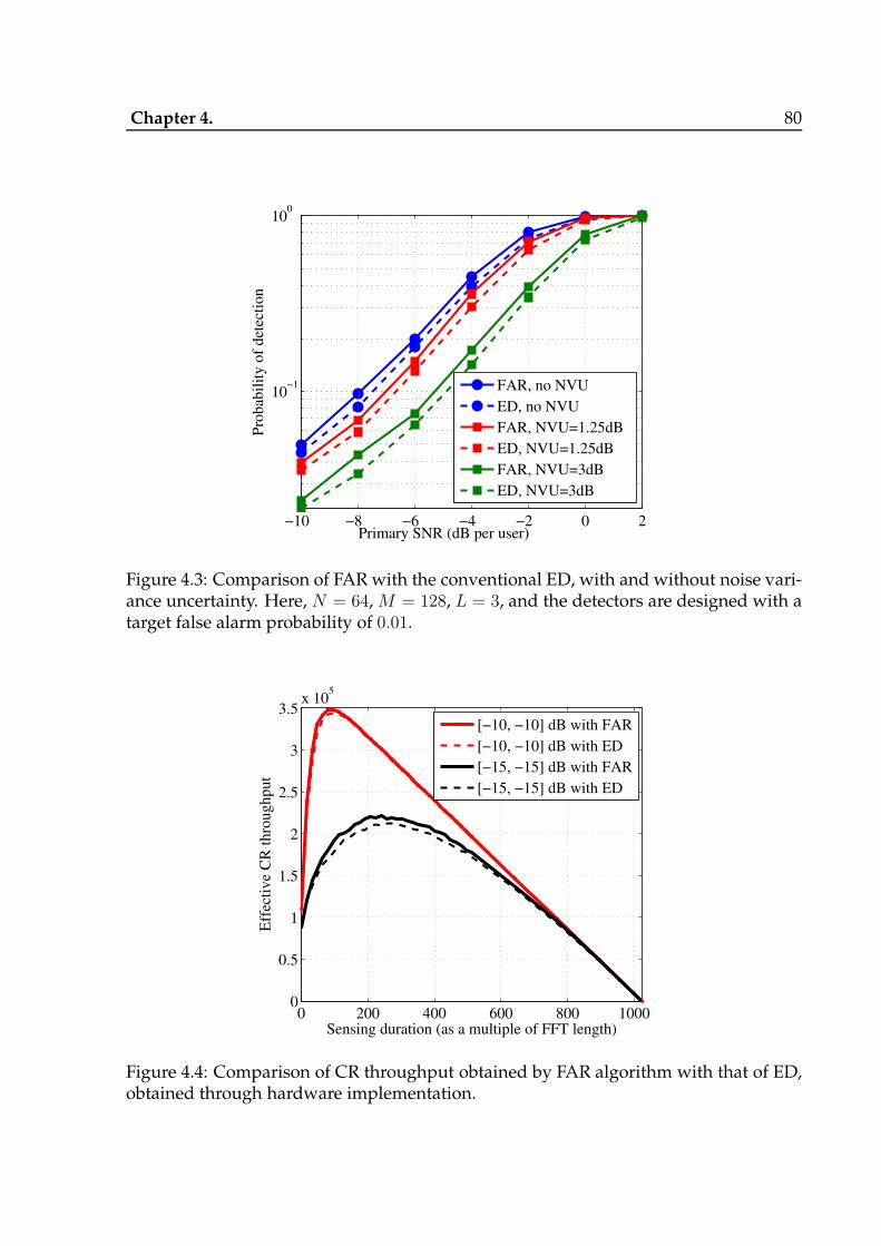
Chapter 4. 80

−10 −8 −6 −4 −2 0 2

10−1

100

Primary SNR (dB per user)

Pro

bab

ilit

y o

f det

ecti

on

FAR, no NVU

ED, no NVU

FAR, NVU=1.25dB

ED, NVU=1.25dB

FAR, NVU=3dB

ED, NVU=3dB

Figure 4.3: Comparison of FAR with the conventional ED, with and without noise vari-ance uncertainty. Here, N = 64,M = 128, L = 3, and the detectors are designed with atarget false alarm probability of 0.01.

0 200 400 600 800 10000

0.5

1

1.5

2

2.5

3

3.5x 10

5

Sensing duration (as a multiple of FFT length)

Eff

ecti

ve

CR

thro

ughput

[−10, −10] dB with FAR

[−10, −10] dB with ED

[−15, −15] dB with FAR

[−15, −15] dB with ED

Figure 4.4: Comparison of CR throughput obtained by FAR algorithm with that of ED,obtained through hardware implementation.

Chapter 4. 81

0.5 0.6 0.7 0.8 0.90

1000

2000

3000

4000

5000

6000

Minimum detection probability Pmin

Eff

ecti

ve

CR

thro

ughput

Sim., SNR=[−1,−1]

Th., SNR=[−1,−1]

Sim., SNR=[−3,−3]

Th., SNR=[−3,−3]

Sim., SNR=[−5,−5]

Th., SNR=[−5,−5]

Figure 4.5: Optimal throughput for N = 64, Nh = 1024. For the simulation result,the optimal throughput was obtained by sweeping a range of M and threshold, andchoosing the pair that offered the best throughput.

0.5 0.6 0.7 0.8 0.90

5

10

15

20

25

Pmin

Op

tim

al M

Th., N=16

Sim., N=16

Th., N=32

Sim., N=32

Th., N=64

Sim., N=64

Figure 4.6: Comparison of optimal number of framesM for different values of the FFTsizeN , for L = 2, andNh = 1024 samples. Notice that asN varies, the optimalM variessuch that NM is roughly the same, for each given Pmin.

Chapter 4. 82

0 0.1 0.2 0.3 0.40

200

400

600

800

1000

1200

1400

1600

Detection threshold

Eff

ecti

ve

CR

thro

ughput

M=1

M=3

M=5

M=7

Figure 4.7: Variation of theoretical throughput Vs. τ , for Nh = 1024, N = 64, withSNR=[−5,−5] dB, and α = [0.5, 0.5] for [C0, C7].

0.2 0.3 0.4 0.5 0.60

0.2

0.4

0.6

0.8

1

Detection threshold

Pro

bab

ilit

y o

f det

ecti

on

Sim., −9.7dB

Sim., −11.7dB

Sim., −13.7dB

Expt., −8.67dB

Expt., −10.67dB

Expt., −12.67dB

Figure 4.8: Comparison of PFA and PD from simulations and experiments, forM = 128at different SNRs. The implementation loss is about 1 dB.

Chapter 4. 83

0 0.2 0.4 0.6 0.8 10

0.2

0.4

0.6

0.8

1

Probability of false alarm

Pro

bab

ilit

y o

f det

ecti

on

Expt., SNR=−8.67dB, M=256

Sim., SNR=−9.7dB, M=256

Expt., SNR=−8.67dB, M=128

Sim., SNR=−9.7dB, M=128

Expt., SNR=−12.67dB, M=256

Sim., SNR=−13.7dB, M=256

Expt., SNR=−12.67dB, M=128

Sim., SNR=−13.7dB, M=128

Figure 4.9: Comparison of ROCs from simulations and experiments, at differentM andSNRs. The implementation loss is about 1 dB.

40 60 80 100 120 140 1600.7

0.75

0.8

0.85

0.9

0.95

1

Sensing duration (as a multiple of FFT length)

Norm

aliz

ed e

ffec

tive

CR

thro

ughput

Expt., Pmin

=0.9

Sims., Pmin

=0.9

Expt., Pmin

=0.7

Sims., Pmin

=0.7

Figure 4.10: OptimumCR throughput Vs. Ns, comparing the hardware implementationwith simulated curves.

Chapter 5

Zero-Crossings Based Spectrum

Sensing Under Noise Uncertainties

5.1 Introduction

One of the key challenges in Cognitive Radios (CR) [1] is Spectrum Sensing (SS), which

is the well-studied binary hypothesis testing problem of determining the presence or

absence of a primary signal in a given frequency band of interest [30, 89]. In the future,

CRs are envisioned to operate in various wireless environments, and in the presence of

interference, changing noise statistics, etc ([62], [30], and references therein). Therefore,

techniques used for SS need to be capable of handling various fading environments,

primary signal models and different types of noise distributions. Hence, the class of

Goodness-of-Fit Tests (GoFT) [51] is a natural choice for SS, where the problem reduces

to accepting or rejecting the noise-only hypothesis, under a constraint on the false alarm

probability. This chapter explores the benefits and drawbacks of GoFTs for CR-SS ap-

plications, in the presence of different types of model uncertainties.

Construction of a GoFT-based detector requires knowledge of the noise statistics. The

84

Chapter 5. 85

noise process in most communications-related applications consists of a Gaussian com-

ponent (also known as the background noise or thermal noise), a controllable interference

component (the so-called class A noise), and an uncontrollable impulsive component

(the so-called class B noise) [55]. Depending on the application and communication

scenario, either class A, class B, or both exist in the noise model. Much of the exist-

ing works in the CR literature consider SS in the Gaussian component alone, i.e., they

assume the noise distribution to be i.i.d. Gaussian. Further, for the most part, the lit-

erature assumes the noise variance to be known [89].1 An exception to this approach

is [108], which studies SS under only non-Gaussian noise model, which ignores the

Gaussian component. However, even if the non-Gaussian component is weak com-

pared to the Gaussian component, the effect of the latter cannot be ignored in prac-

tice [55]. Another important aspect for the SS design is the need for knowledge of the

parameters of the noise model, such as its variance [38,55,109–111]. Therefore, the per-

formance of SS is affected by the two kinds of uncertainties in the knowledge of the

noise: imperfect knowledge of the parameters of the distribution, which we refer to as

Noise Parameter Uncertainty (NPU), and imperfect knowledge of the distribution itself,

which we refer to as Noise Model Uncertainty (NMU). Additionally, in many scenarios,

the noise process may be correlated either spatially or temporally [112], or due to digi-

tal filtering at the receiver [113]. To the best of authors’ knowledge, SS under the above

stated noise uncertainties, and GoFT under colored noise is not addressed in the GoFT

based SS literature so far.

1The GoFT literature for testing against Gaussianity spans over a century now, and is an active areaof research even today. A brief survey of the well-known and widely used techniques is presented inAppendix E.

Chapter 5. 86

Energy Detection (ED) is a simple technique for SS, where the signal energy in the

frequency of interest is measured over a sensing duration and compared to a threshold.

However, in the presence of the background noise alone, it performs poorly in the low

SNR regime under the NPU [38]. In the presence of the non-Gaussian components, ED

fails to satisfy the false-alarm probability constraint because of the underlying heavy-

tailed, non-Gaussian distribution with infinite variance. Recently, an Anderson-Darling

statistic [114] based test (ADD) [52] and an Ordered Statistics based Detector (OSD)

[54] were proposed, which outperform ED (in the Neyman-Pearson sense) when the

primary signal is a constant with Rayleigh fading and i.i.d. Gaussian noise, with known

variance. However, because of the underlying assumptions and construction, ADD and

OSD are susceptible to both NPU and NMU. The Blind Detector (BD), proposed in [53],

is robust to NPU, but only handles i.i.d. Gaussian noise, i.e., it is not robust to NMU.

In this chapter, a detector calledweighted Zero-Crossings Detector (WZCD), based on the

Zero-Crossings (ZC) and Higher Order Crossings (HOC) in the received observations

is proposed, which is a generalization of a detector proposed by Kedem and Slud [115].

The main contributions of this chapter are

• A weighted ZC based detector is proposed. Given a target false alarm probabil-

ity, near-optimal detection thresholds are obtained for uniform and exponential

weights (Sec. 5.4).

• The proposed detector is shown to be robust to both NMU and NPU (Sec. 5.5).

• For the specific case where the noise has two components namely the background

component and class A component and with both components being modeled by

Gaussian distribution with different variances, it is analytically shown that the ED

Chapter 5. 87

and ADD do not satisfy the given false-alarm constraint. The actual applicability

and utility/efficacy of the BD, which is much wider than that discussed in [53] is

highlighted.

• Under colored noise, the expected number of ZCs and HOCs when the noise dis-

tribution is Gaussian, are derived through a generalized level-crossings lemma

(Sec. 5.6). The robustness of the proposed detector to both NMU and NPU in the

case of colored noise is discussed.

• In a detailed simulation study, the performance of the proposed detectors is com-

pared with the BD under various primary signal models operating in different

noise and fading environments (Sec. 5.7).

Thus, we conclude, in Sec. 5.9, that the proposed WZCD is a promising technique for

detecting primary signals at low SNR, under both NPU and NMU.

We start by describing the system model.

5.2 SystemModel

Consider a CR node with M observations denoted by Yi, i ∈ M , 1, 2, · · · ,M. It is

assumed that each Yi is real valued ([52, 53]). In the GoFT formulation, the problem is

to either reject or accept the null hypothesis

H0 : Yi ∼ fN, i ∈ M

Chapter 5. 88

and the threshold is chosen such that a constraint αf ∈ [0, 1] on the probability of false

alarm is satisfied, i.e.,

pf , Preject H0|H0 is true ≤ αf . (5.1)

Here, fN represents the distribution of the noise process, i.e., the distribution of Yi under

H0. First, consider the case where the noise observations are i.i.d. Following Middle-

ton [55], the observations underH0 are modeled as

Yi = Y(G)i + Y

(A)i + Y

(B)i , i ∈ M, (5.2)

where the Gaussian component Y(G)i ∼ fG

d.= N (0, σ2

G), and N (µ, σ2) represents a Gaus-

sian distribution with mean µ and variance σ2. The class A and B noise components are

denoted by Y(A)i and Y

(B)i , respectively. Middleton has shown that the PDF of class B

component alone can be well-approximated by a two-parameter symmetric α-stable

(SαS) distribution, i.e., the characteristic function of Y(B)i , denoted by ΦB , is given

by [55, eq. (88)]

ΦB(ω, γ0, α) = exp (−γ0|ω|α) , γ0 > 0, 0 < α ≤ 2. (5.3)

Vastola [109] has shown that the PDF of Y(G)i + Y

(A)i can be well-approximated by the

ǫ-mixture model [110]. Using this approximation, we can write

Y(G)i + Y

(A)i ∼ (1− ǫ)fG + ǫfI , (5.4)

where fI represents a distribution which has heavier tails as compared to fG , for ex-

ample, a Laplace distribution [110], or another Gaussian distribution with a variance

Chapter 5. 89

larger than that of fG [111]. Typically, σ2I , the variance of fI , satisfies σ2

I ≫ σ2G. The

mixing parameter 0 < ǫ ≪ 1 depends on the parameters of the PDF of the class A

model ([55], [109]).

In this chapter, our aim is to design a GoFT that is robust to the following two noise

uncertainties:

1. The noise model uncertainty (NMU) is caused due to the imperfect knowledge of

noise distribution fN. The presence of either class A, B or both in fN depends

on the physical environment [55, Tab. I]. Also, the distribution of fI in (5.4)

can be modeled to be Gaussian, Laplace, or Cauchy ([110], [111]). However, the

background Gaussian noise is always present [55].

2. The noise parameter uncertainty (NPU) arises due to the inaccurate knowledge of

the parameters infN, i.e., σ2G [38], σ2

I [110], ǫ [109], and α [55].

In the following section, we present a brief note on some of the existing GoFTs, pro-

posed and studied in the context of SS in CR.

5.3 Existing GoFT for Spectrum Sensing

5.3.1 Energy Detector (ED)

The ED can be proposed as a GoFT, and has the following critical region

Y1, Y2, · · · , YM ∈ R

M : E ,M∑

i=1

Y 2i > τED

, (5.5)

where τED is the detection threshold, chosen such that the pf is at a given desired level

α. In particular, when the observations are i.i.d. and fN = fGd.= N (0, σ2

G) with a known

Chapter 5. 90

σ2G, the statistic E is chi-square distributed with 2M degrees-of-freedom. In this case, it

is easy to show that

τED = γ−1inc

(1− α,

M − 1

2,2σ2

G

M

), (5.6)

where γ−1inc (x,A,B) represents the normalized inverse gamma cumulative distribution

function evaluated at x, with parameters A and B [116].

5.3.2 Anderson-Darling Statistic Based Detector (ADD)

The Anderson-Darling statistic [114] based GoFT was proposed in the CR context by

Wang et al. [52]. When fN is completely known (with i.i.d. observations, and known

variance), and the observations are ordered such that Y1 ≤ Y2 ≤ · · · ≤ YM , the Anderson-

Darling statistic is defined as

A2c,M , −

∑Mi=1(2i− 1)(lnZi + ln(1− ZM+1−i))

M−M (5.7)

with Zi , FN, the CDF of noise observations. The ADD has the following critical region

[52]

Yi, i ∈ M : A2

c,M ≥ τADD

, (5.8)

where τADD is chosen such that pf is set to a level α. For a given α, and for moderate

values ofM , τADD satisfies [52]:

1−√2π

τADD

∞∑

ℓ=0

(−1)ℓΓ(0.5 + ℓ)

Γ(0.5)ℓ!exp

(−π

2(4ℓ+ 1)2

8τADD

)

× (4ℓ+ 1)

∫ ∞

0

exp

(τADD

8(w2 + 1)− π2w2(4ℓ+ 1)2

8τADD

)dw =α. (5.9)

A table of thresholds for different values of pf is given by Stephens [117].

Chapter 5. 91

5.3.3 Blind Detector (BD)

The BD was proposed by Shen et al. [53] as a robust detector under noise uncertainty.

When fN = fGd.= N (0, σ2

G), the construction of the BD is such that the test statistic is

independent of σ2G. M observations are divided into n windows of m observations

each, and the test statistic is constructed as follows. Define

Xl ,m−1∑

u=0

Yml−um

, S2l ,

m−1∑

u=0

(Yml−u −Xl)2

m− 1, (5.10)

and Bl ,Xl

Sl/√m, l = 1, · · · , n. (5.11)

Now, the Anderson-Darling statistic is formed based on Bl, l = 1, · · · , n using (5.7),

which is defined as

A2c,n , −

∑ni=1(2i− 1)(lnCi + ln(1− Cn+1−i))

n− n, (5.12)

where Cl = Fs(Bl), where Fs represents the CDF of a student-t distributed random

variable with parameterm− 1. Observe that Fs does not depend σ2G. Therefore, the BD

is robust to noise variance uncertainty, and has the following critical region

Yi, i ∈ M : A2

c,n ≥ τBD

. (5.13)

For large enough n, the optimal threshold τBD is calculated in a similar way to ADD,

using (5.9).

Remark: In our simulations, we have found that BD can be applied even in much

weaker scenarios that those noted by Shen et al [53]. In this chapter, along with a new

zero-crossings based detector, we also present an analysis of BD that captures some of

Chapter 5. 92

its key strengths. The applicability of BD is discussed in Appendix D.4.

In the next section, we propose a detector based on the weighted Zero-Crossings (ZC)

in the observations Yi, i ∈ M. We discuss the robustness of the proposed detector to

both NMU and NPU in Sec. 5.5.

5.4 Weighted Zero-Crossings Based Detection

Zero-crossings based detection was first proposed by Kedem and Slud [115] as a sim-

ple non-parametric detection strategy for testing against Gaussian samples. Here, we

generalize this approach by considering zero-crossings, and study its performance in

the presence of NMU and NPU. In our simulations, for a large class of primary signal

models, the first few values of ∆k,M were found to be significantly larger than those

for higher values of k. Therefore, if the weights are chosen such that the lower order

ZCs are weighed larger than the higher order ZCs, the detection performance can be

significantly improved. The corresponding test statistic is constructed as follows. Let

∇k denote the kth order difference operator on Yi, defined as

∇Yi , Yi − Yi−1

∇2Yi = ∇(∇Yi) = Yi − 2Yi−1 + Yi−2

...

∇kYi =

k∑

j=0

(k

j

)(−1)jYi−j, i ≥ k + 1. (5.14)

Chapter 5. 93

A kth order zero-crossing in the observations Yi, i ∈ M is said to occur if the sign of

∇k−1Yi is different from that of∇k−1Yi+1. LetDk,M denote the number of kth order zero-

crossings across M samples. Note that, we define ∇0Yi , Yi. Now, let ∆j,M , and µj,M

be defined as

∆j,M ,

D1,M , j = 1,

Dj,M −Dj−1,M , j = 2, · · · , k − 1

(M − 1)−Dk−1,M , j = k,

(5.15)

µj,M , E∆j,M , j = 1, · · · , k, (5.16)

where E(·) denotes the expectation operator. Observe that∑k

j=1∆j,M = M − 1. A

goodness-of-fit measure Ψ2w up to a given order k can be defined as

Ψ2w ,

k∑

j=1

wj(∆j,M − µj,M)2

µj,M. (5.17)

For a given set of weights wj , a Ψ2w Statistic based Detector (ΨwSD) is given by

Ψ2w

≁H0

≷∼H0

τΨ

w, (5.18)

and τΨwis chosen such that PΨ2

w > τΨw|H0 ≤ αf , for some target false alarm probabil-

ity αf ∈ [0, 1]. We refer to the detector based on (5.17) as aWeighted Zero-Crossings based

Detector (WZCD). Note that, when wj = 1, j = 1, 2, . . . , k, the detector reduces to the

classical ZCD [115].

Now, as seen from (5.16) and (5.17), for a specific set of weights, the construction of

the WZCD depends only on the knowledge of µj,M for j = 1, 2, · · · . When fN = fGd.=

Chapter 5. 94

N (0, σ2G), for moderately largeM , it is known that [118]

EDk,M = (M − 1)

1

2+

1

πsin−1

(k − 1

k

), (5.19)

Hence, µk,M can be easily calculated by substituting (5.19) in (5.15) and (5.16). Also, it

has been observed that for most processes, calculating and using D1,M , · · · , D8,M , i.e.,

up to k = 8 are enough, in the sense that for k > 9, the ZCs do not contribute much to

the performance [118].

Next, we consider the following two cases.

A) Equal and unit weights: The past work [115] studied the statistic in (5.17) for wj =

1, j = 1, · · · , k, which will be denoted as Ψ21. It was observed that the PDF of Ψ2

1 is

approximately the same for any discrete-time stationary ARMA process, and hence can

be used to construct a GoFT against any such process. Additionally, it is known that

for moderately largeM , the Ψ21 statistic can be approximated by a Pearson type III (chi-

squared or gamma) distribution [118]. These PDF approximations have been studied

in detail earlier, and are known to be highly accurate [119]. In particular,

Ψ21 ∼ χ2

3(11), (5.20)

where χ2D(λ) is a non-central chi-square distribution with D degrees of freedom and

non-centrality parameter λ. Hence, for a given target false alarm probability αf , the

detection threshold corresponding to using Ψ21, denoted by τΨ

1, satisfies

Q 32

(√11,√τΨ1

)=αf , (5.21)

where Qκ(·, ·) represents the Marcum-Q function of order κ.

Chapter 5. 95

B) Exponential weights: Asmentioned earlier, in our simulations, we found that weigh-

ing the lower order ZCs higher than the higher order ZCs can lead to significantly

better performance. Motivated by this, we consider the exponential weighting case,

i.e., wj , e−(j−1). Let the corresponding WZCD test statistic be denoted byΨ2e. Through

simulations, it was observed that the tail of the distribution ofΨ2e follows closely to that

of an F-distribution with parameters 17.5 and 7 (denoted by F(17.5, 7)), for moderately

largeM . The loss due to this approximation is negligible, and is quantified in the Sec.

5.7. Therefore, for a test based on Ψ2e, the near-optimal detection threshold τΨ

e satisfies

1− I(

17.5τmΨSD

17.5τmΨSD + 7, 8.75, 3.5

)= αf , (5.22)

where I(κ, a, b) represents the regularized incomplete beta function with parameters

κ, a and b [116].

We note that the optimal threshold calculation for ADD [52] and BD [53] require the

evaluation of an integral of an infinite series, which is computationally intensive, as

opposed to the single integral calculation in (5.21) and (5.22).

To summarize, the detection procedure using the WZCD is as follows:

1. Fix k = 9. CollectM =M ′ + k observations, Yi.

2. Calculate the first-k ZCs andHOCs of Yi using (5.14). Using (5.19), calculate the

expected zero-crossings. Denote this by µ(g).

3. Construct the statistic Ψ2w for appropriately chosen weights.

4. Compare Ψ2w to τΨ

w. For unit and exponential weights, use τΨ

1, and τΨ

efrom (5.21)

and (5.22), respectively. Declare H0 if Ψ2w < τΨ

w , and not H0 otherwise.

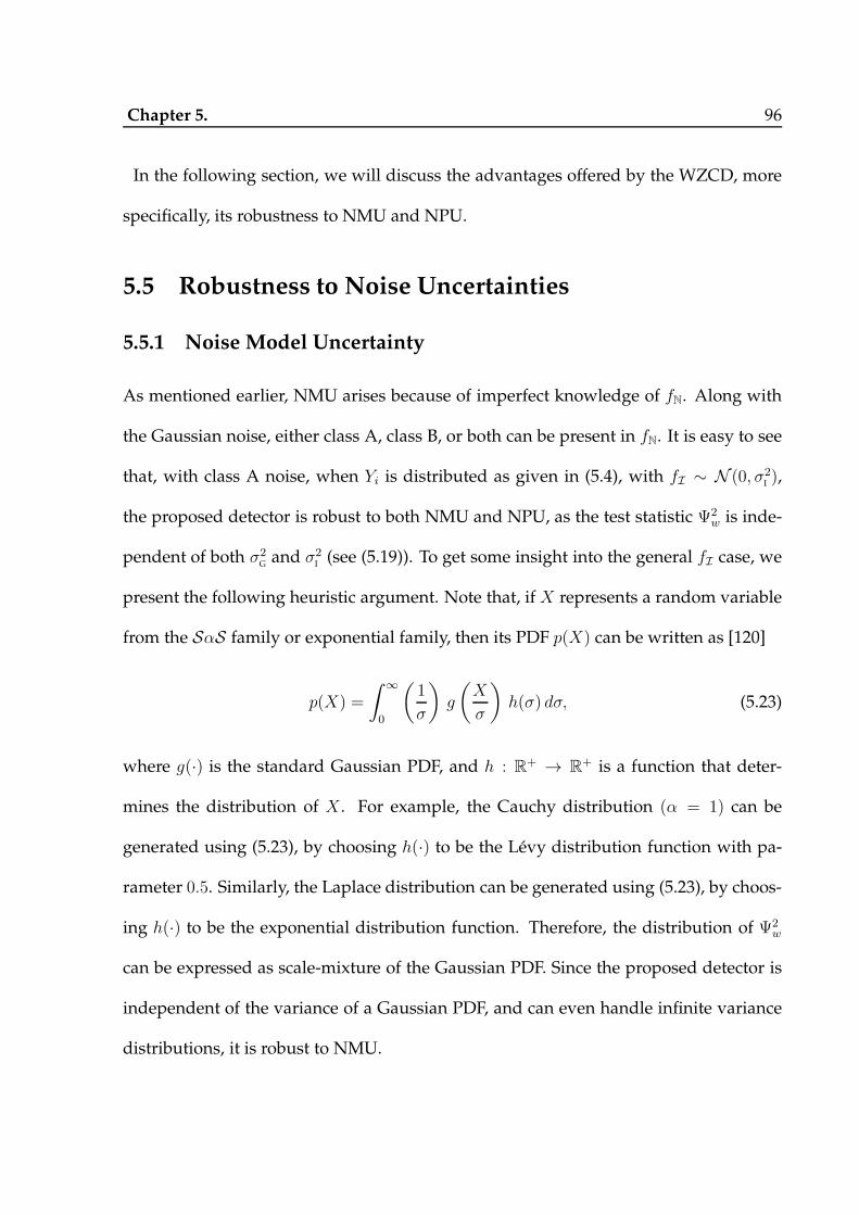
Chapter 5. 96

In the following section, we will discuss the advantages offered by the WZCD, more

specifically, its robustness to NMU and NPU.

5.5 Robustness to Noise Uncertainties

5.5.1 Noise Model Uncertainty

As mentioned earlier, NMU arises because of imperfect knowledge of fN. Along with

the Gaussian noise, either class A, class B, or both can be present in fN. It is easy to see

that, with class A noise, when Yi is distributed as given in (5.4), with fI ∼ N (0, σ2I ),

the proposed detector is robust to both NMU and NPU, as the test statistic Ψ2w is inde-

pendent of both σ2G and σ2

I (see (5.19)). To get some insight into the general fI case, we

present the following heuristic argument. Note that, if X represents a random variable

from the SαS family or exponential family, then its PDF p(X) can be written as [120]

p(X) =

∫ ∞

0

(1

σ

)g

(X

σ

)h(σ) dσ, (5.23)

where g(·) is the standard Gaussian PDF, and h : R+ → R+ is a function that deter-

mines the distribution of X . For example, the Cauchy distribution (α = 1) can be

generated using (5.23), by choosing h(·) to be the Levy distribution function with pa-

rameter 0.5. Similarly, the Laplace distribution can be generated using (5.23), by choos-

ing h(·) to be the exponential distribution function. Therefore, the distribution of Ψ2w

can be expressed as scale-mixture of the Gaussian PDF. Since the proposed detector is

independent of the variance of a Gaussian PDF, and can even handle infinite variance

distributions, it is robust to NMU.

Chapter 5. 97

5.5.2 Noise Parameter Uncertainty

Since every distribution in the SαS and exponential families can be generated as scale-

mixture of Gaussian distributions, whenM is sufficiently large, theWZCD can bemade

robust to uncertainty in the parameter set (α, ǫ, fI , σ2I ). Intuitively, the number of ZCs

in the observations for a unimodal, symmetric distribution is approximatelyM/2, irre-

spective of its variance. That is, the probability that the distribution would take pos-

itive values will be approximately 0.5. Therefore, for large M , the distribution of the

test statistic defined by (5.17) is approximately the same for all such symmetric distri-

butions, thus making the statistic relatively independent of the parameters of the noise

such as its variance.

In the following, we will show that ED and ADD do not satisfy their respective false-

alarm constraints, even in the case where class B model is not present in fN. It is

straightforward to see that when fG and fI areN (0, σ2G) and N (0, σ2

I ) respectively, fN ∼

N (0, ǫσ2G + (1− ǫ)σ2

I ). As already seen, since the the statistics under BD and WZCD are

not dependent on the Gaussian noise variance, they still meet the required false-alarm

constraint, and their probability of detection remains unchanged. However, ED and

ADD do not satisfy false-alarm constraints, as highlighed below.

Result 2. Under the presence of only class A noise in fN, when fI is N (0, σ2I ), and when ED

and ADD are designed oblivious to the presence of the impulsive noise i.e., their thresholds

are fixed for fG , while the observations have the distribution fN, they satisfy their respective

false-alarm constraints if and only if ǫ = 0.

In Appendix D.3, we will provide a sketch of the proof of the above result.

Chapter 5. 98

5.6 Expected HOCs for Correlated Gaussian Noise

In this section, we discuss the applicability of the WZCD for the case when the noise-

only observations are correlated, and follows a Gaussian distribution. From the discus-

sions in earlier section, for ΨeSD and Ψ1SD, µj,M , j = 1, · · · , k and the distribution of

Ψ2 statistic needs to be known. In the following, we derive a lemma which gives ana-

lytical expressions for the expected level-crossings in a Gaussian, correlated process of

which, the expected zero-crossings is a special case. Later, some comments on the case

of general fN, and the effect of NMU and NPU are studied.

Consider the case where the noise process is a (p, q) ordered Auto-Regressive Moving-

Average (ARMA) Gaussian, i.e., fNd.= fG , with a correlation matrix RG. When RG is

known, µj,M can be obtained in closed form, as shown through the following general

Level-Crossings (LC) lemma, which highlights the connection between the expected

number of LC (at any level ℓ) of a Gaussian process of known correlation structure and

its normalized autocorrelation function. The expected number of ZC is a special case of

this result, for ℓ = 0.

Lemma 3. For the observations Y1, Y2, · · · , YM from a known, stationary, Gaussian process

fG(y;RG), the expected number of level crossings for any given level ℓ is given by

ED1,M = 2(M − 1)Q(ℓ)(1−Q(ℓ))(1− ρX), (5.24)

where Q(·) is the Gaussian Q-function, and ρX is the first order normalized autocorrelation

Chapter 5. 99

value of a process Xi, i ∈ M which is defined as

Xi ,

1, Yi > ℓ,

0, Yi ≤ ℓ, i ∈ M, and(5.25)

ρX ,cov(Xi, Xi+1)

var(Xi)=

EXiXi+1 − EXiEXi+1

var(Xi)(5.26)

where cov(·, ·) and var(·) denote the cross- and auto-covariance functions, respectively.

Proof. See Appendix D.1.

Corollary 4. For ℓ = 0, the result in (5.24) reduces to a known result on the expected number

of ZCs [118]

ED1,M = (M − 1)

(1

2− 1

πsin−1 ρ1,G

), (5.27)

where ρ1,G is the first order normalized autocorrelation of fG(y;RG), given by

ρ1,G ,cov(Yi, Yi+1)

var(Yi), i ∈ M (5.28)

Therefore, the expected number of first order ZCs depends on ρ1,G.

Proof. See Appendix D.2.

Since Yi, i ∈ M are Gaussian, ∇kYi are also Gaussian for all k. Using this property

and above result for ℓ = 0, Kedem has shown that the HOC depends on ρ2,G, · · · , ρM−1,G

as [118]

cos

(πEDk+1,M

M − 1

)=

∇2kρk−1,G

∇2kρk,G, (5.29)

where ∇(·) operates on the sequence ρk,G, k = 1, 2, · · · .

Chapter 5. 100

Now, consider the general case, where the noise-only observations are correlated and

distributed as fN along with the presence of class A and B models. As in the previ-

ous case, we can argue that the distribution of background noise and class A compo-

nent combined follows a correlated Gaussian distribution. Also, let the implusive noise

(class B) follow a correlated SαS distribution. Similar to the case of i.i.d. observations

discussed in Sec. 5.5, even in this case, approximating the non-Gaussian noise mod-

els as a mixture Gaussian process is found to be sufficiently accurate [121]. Hence, the

WZCD is robust to both NMU and NPU, even for correlated observations.


5.7.1 Performance Under I.I.D. Noise

The suitability of a GoFT in the context of SS in a CR can only be validated through

extensive simulations, i.e., by studying its performance against various primary signal

models, and different channel conditions. We consider a Rayleigh fading channel from

the primary transmitter to the CR node; the number of observations M = 300, and

target false alarm probability pf = 0.05. The channel gain is assumed to remain constant

throughout the M observations. For the primary signal, we consider the following

models, with SNR = −5 dB in all experiments:

1. Model 1 - constant primary: The primary signal is a known constant. This model

was considered previously in the GoFT for SS [52], [53].

2. Model 2 - sinusoidal primary: This simulates the scenario where the primary sig-

nal contains a strong pilot tone signal at a known frequency, similar to pilot-based

Chapter 5. 101

detection in Digital TV (IEEE 802.22) signals [56,122]. The frequency of the signal

is set to be 4kHz.

We have fixed σ2G = 1. The uncertainty in σ2

G, i.e., the noise variance uncertainty is

assumed to be 3 dB [38], [123]. For the class B noise model, we let γ0 = 1/√2. Note

that the value of γ0 matters only when α = 2, i.e., when the distribution is Gaussian,

in which case its variance is 2γ20 = 1. For the BD, we set the number of windows as

m = 30 [53].

Consider SS under the class B (SαS) and Gaussian noise under hypothesis H0. In Fig.

5.1, the performance of all the detectors for constant primary is shown, with varying α.

It is seen that around 1 ≤ α ≤ 2, BD outperforms the proposed detectors. However,

as α reduces, the performance of BD deteriorates and approaches the pf = pd line.

Therefore, when α is low, BD does not satisfy the false alarm constraint. However,

under model 2, both the proposed detectors outperform BD and satisfy the required

false alarm constraint. This is shown in Fig. 5.2.

Now, consider detection under class A model with the Gaussian noise, i.e., the ǫ-

mixture model. In Fig. 5.3, the performance of the detectors is shown as a function of

σ2I , with fI modeled as i.i.d. Gaussian, and for ǫ = 0.05. It is seen that the performance

of all the detectors remains constant for different values of σ2I and ǫ. In all the cases,

the performance of Ψ1SD and ΨeSD are comparable to that of BD under primary signal

model 1, and improves significantly relative to that of BD under model 2. A similar

trend is observed under the same setup with the fI beingmodeled as Laplacian, as seen

in Fig. 5.4. This shows that the performance of all the detectors designed for Gaussian

noise are also valid under Laplacian noise, and with similar performance trends.

Chapter 5. 102

Figure 5.5 shows the performance of BD, Ψ1SD and ΨeSD under i.i.d. Gaussian noise

alone, and when the primary signal follows Models 1 and 2. Under Model 1, it is seen

that BD performs better than Ψ1SD and ΨeSD, especially in the low SNR regime. This

is expected, as the underlying Anderson-Darling statistic of BD is powerful for testing

against mean change in Gaussian signals [114]. However, it is seen that Ψ1SD and

ΨeSD outperform the BDwhen the primary signal followsModel 2. Additionally,ΨeSD

performs better than Ψ1SD. In Fig. 5.6, the performance of the detectors are plotted

with correlated Rayleigh fading with the correlation modeled as a first order Auto-

Regressive (AR) model [124] with ρ = 0.5, under i.i.d. Gaussian noise alone. It is seen

that ΨeSD outperforms all the detectors. These simulations confirm that the proposed

detectors are well suited for testing pilot based signals; for example, under a setup

similar to the primary signal detection in IEEE 802.22 DTV standard.

Finally, in Figs. 5.7 and 5.8, the performance of the detectors under all the noise mod-

els combined is plotted, for both primary models. The results seen earlier, for the class

B noise model with Gaussian noise, hold in these cases as well. There is a performance

degradation due to presence of the heavy-tailed class A noise component, but the per-

formance of Ψ1SD and ΨeSD are better than the chance line. For the same setup, Fig.

5.9 shows the agreement between theoretical and simulated threshold values for all the

detectors, thereby validating our analysis in (5.21) and (5.22).

As a final remark, we note that, due to the CFARproperty of BD,Ψ1SD, andΨeSD (and

any detector from the WZCD family), they fail to distinguish between the hypotheses

when the primary signal has the same distribution as the noise process, with a different

variance. Then, all the detectors would operate on the chance line (pf = pd line), for all

Chapter 5. 103

SNR values. Therefore, for this particular case, WZCD is not a viable choice.

5.7.2 Performance Under Colored Noise

In the case of colored noise, ZCs and HOCs can be obtained by using the generalized

level crossings lemma. However, the distribution of the statistics Ψ2M for both uniform

and equal, and exponential weights are not known in closed form and the optimal

thresholds need to be obtained through numerical techniques, provided the correlation

structure is correctly known. The ADD and BD cannot be applied here, because their

design is valid only for the i.i.d. case [114]. In this section, the performance of ED,Ψ1SD

and ΨeSD are considered in the following scenarios, where the noise observations are

correlated. For the following results, we assume an uncertainty in the knowledge of

EY 2i , 1 ≤ i ≤M , of 3dB.

Correlation Model C1

In this section, we study the performance of WZCD when the noise observations are

correlated with a constant correlation coefficient. Such a correlation model is observed

in, for e.g., an antenna array, where the correlation structure depends on the impedances

of the antennas ( [125], [112]). Also, with this model, fast fading is considered in un-

der the signal-present hypothesis, where the fading gains are different and i.i.d. across

each observation. The performance of the detectors under such correlated noise is as

shown in Fig. 5.10. It is observed that both Ψ1SD and ΨeSD outperform ED. Under

constant primary, the performances of both Ψ1SD and ΨeSD decrease as the noise cor-

relation increases. However, under model 2, the performance of both Ψ1SD and ΨeSD

first decrease with the correlation value, and later increases.

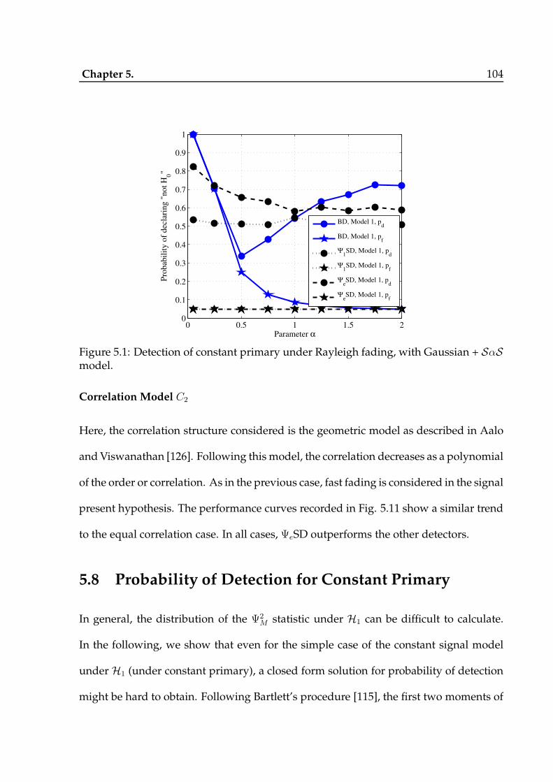
Chapter 5. 104

0 0.5 1 1.5 20

0.1

0.2

0.3

0.4

0.5

0.6

0.7

0.8

0.9

1

Parameter α

Pro

bab

ilit

y o

f dec

lari

ng "

not

H0"

BD, Model 1, pd

BD, Model 1, pf

Ψ1SD, Model 1, p

d

Ψ1SD, Model 1, p

f

ΨeSD, Model 1, p

d

ΨeSD, Model 1, p

f

Figure 5.1: Detection of constant primary under Rayleigh fading, with Gaussian + SαSmodel.

Correlation Model C2

Here, the correlation structure considered is the geometric model as described in Aalo

andViswanathan [126]. Following this model, the correlation decreases as a polynomial

of the order or correlation. As in the previous case, fast fading is considered in the signal

present hypothesis. The performance curves recorded in Fig. 5.11 show a similar trend

to the equal correlation case. In all cases, ΨeSD outperforms the other detectors.

5.8 Probability of Detection for Constant Primary

In general, the distribution of the Ψ2M statistic under H1 can be difficult to calculate.

In the following, we show that even for the simple case of the constant signal model

under H1 (under constant primary), a closed form solution for probability of detection

might be hard to obtain. Following Bartlett’s procedure [115], the first two moments of

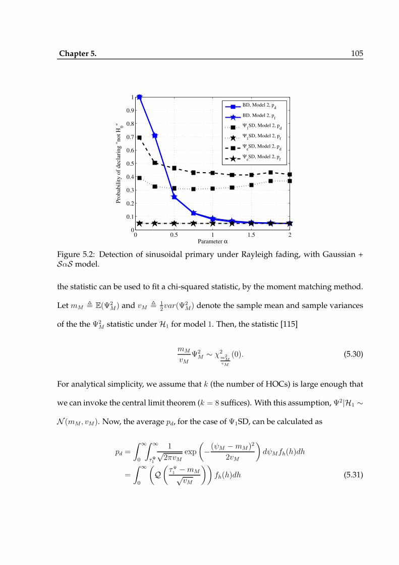
Chapter 5. 105

0 0.5 1 1.5 20

0.1

0.2

0.3

0.4

0.5

0.6

0.7

0.8

0.9

1

Parameter α

Pro

bab

ilit

y o

f dec

lari

ng "

not

H0"

BD, Model 2, pd

BD, Model 2, pf

Ψ1SD, Model 2, p

d

Ψ1SD, Model 2, p

f

ΨeSD, Model 2, p

d

ΨeSD, Model 2, p

f

Figure 5.2: Detection of sinusoidal primary under Rayleigh fading, with Gaussian +SαS model.

the statistic can be used to fit a chi-squared statistic, by the moment matching method.

Let mM , E(Ψ2M) and vM , 1

2var(Ψ2

M) denote the sample mean and sample variances

of the the Ψ2M statistic underH1 for model 1. Then, the statistic [115]

mM

vMΨ2M ∼ χ2

m2M

vM

(0). (5.30)

For analytical simplicity, we assume that k (the number of HOCs) is large enough that

we can invoke the central limit theorem (k = 8 suffices). With this assumption, Ψ2|H1 ∼

N (mM , vM). Now, the average pd, for the case of Ψ1SD, can be calculated as

pd =

∫ ∞

0

∫ ∞

τΨ1

1√2πvM

exp

(−(ψM −mM)2

2vM

)dψMfh(h)dh

=

∫ ∞

0

(Q(τΨ1−mM√vM

))fh(h)dh (5.31)

Chapter 5. 106

10 20 30 40 50 60 70 80 90 1000.1

0.2

0.3

0.4

0.5

0.6

0.7

0.8

0.9

σI

2

Pro

bab

ilit

y o

f dec

lari

ng "

not

H0"

BD, Model 1Ψ

1SD, Model 1

ΨeSD, Model 1

BD, Model 2Ψ

1SD, Model 2

ΨeSD, Model 2

Figure 5.3: Detection of primary models 1 and 2 under Rayleigh fading, with ǫ-mixturemodel, ǫ = 0.05, and fI ∼ N (0, σ2

I ).

where fh(·) is the PDF of the channel. Note thatmM and vM are functions of the channel

gain h. A similar analysis can be carried out for the ΨeSD, in which case the probability

of detection p(m)d is given by

p(m)d =

∫ ∞

0

Q

τ

Ψe−m

(m)M√

v(m)M

fh(h)dh, (5.32)

where m(m)M , E(mΨ

2), and v(m)M , 1

2var(mΨ

2). The agreement between theoretical and

simulated values of pm is shown in Fig. 5.12, where we have numerically evaluated the

integral. It is seen that the agreement becomes tighter as SNR increases. Alternatively,

the Q function can be approximated by an exponential term, to evalute the integral in

closed form, as suggested by Lopez-Benitez and Casadevall [66].

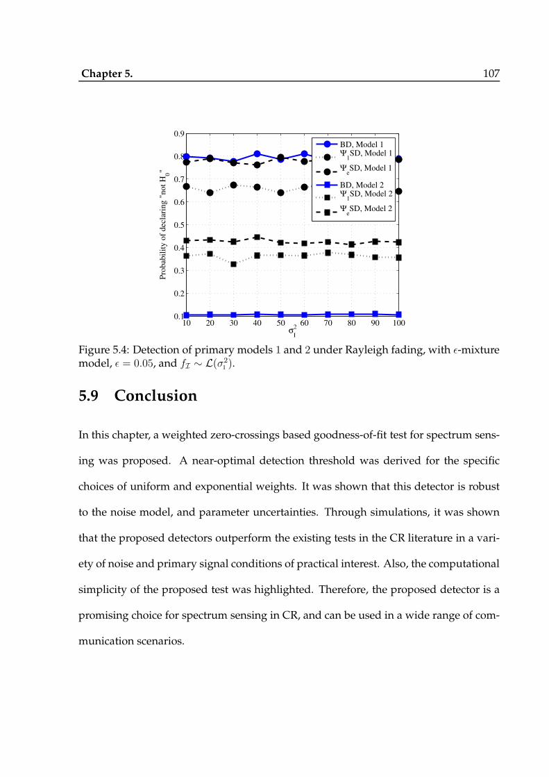
Chapter 5. 107

10 20 30 40 50 60 70 80 90 1000.1

0.2

0.3

0.4

0.5

0.6

0.7

0.8

0.9

σI

2

Pro

bab

ilit

y o

f dec

lari

ng "

not

H0"

BD, Model 1Ψ

1SD, Model 1

ΨeSD, Model 1

BD, Model 2Ψ

1SD, Model 2

ΨeSD, Model 2

Figure 5.4: Detection of primary models 1 and 2 under Rayleigh fading, with ǫ-mixturemodel, ǫ = 0.05, and fI ∼ L(σ2

I ).

5.9 Conclusion

In this chapter, a weighted zero-crossings based goodness-of-fit test for spectrum sens-

ing was proposed. A near-optimal detection threshold was derived for the specific

choices of uniform and exponential weights. It was shown that this detector is robust

to the noise model, and parameter uncertainties. Through simulations, it was shown

that the proposed detectors outperform the existing tests in the CR literature in a vari-

ety of noise and primary signal conditions of practical interest. Also, the computational

simplicity of the proposed test was highlighted. Therefore, the proposed detector is a

promising choice for spectrum sensing in CR, and can be used in a wide range of com-

munication scenarios.

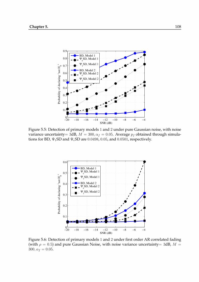
Chapter 5. 108

−20 −18 −16 −14 −12 −10 −8 −6 −40

0.1

0.2

0.3

0.4

0.5

0.6

0.7

0.8

0.9

SNR (dB)

Pro

bab

ilit

y o

f dec

lari

ng "

not

H0"

BD, Model 1Ψ

eSD, Model 1

Ψ1SD, Model 1

BD, Model 2Ψ

eSD, Model 2

Ψ1SD, Model 2

Figure 5.5: Detection of primary models 1 and 2 under pure Gaussian noise, with noisevariance uncertainty= 3dB,M = 300, αf = 0.05. Average pf obtained through simula-tions for BD, Ψ1SD and ΨeSD are 0.0498, 0.05, and 0.0501, respectively.

−20 −18 −16 −14 −12 −10 −8 −6 −40

0.1

0.2

0.3

0.4

0.5

0.6

SNR (dB)

Pro

bab

ilit

y o

f dec

lari

ng "

not

H0"

BD, Model 1Ψ

eSD, Model 1

Ψ1SD, Model 1

BD, Model 2Ψ

eSD, Model 2

Ψ1SD, Model 2

Figure 5.6: Detection of primary models 1 and 2 under first order AR correlated fading(with ρ = 0.5) and pure Gaussian Noise, with noise variance uncertainty= 3dB, M =300, αf = 0.05.

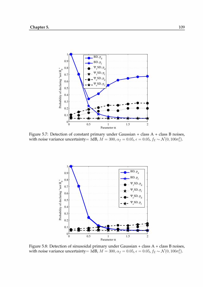
Chapter 5. 109

0 0.5 1 1.5 20

0.1

0.2

0.3

0.4

0.5

0.6

0.7

0.8

0.9

1

Parameter α

Pro

bab

ilit

y o

f dec

lari

ng "

not

H0"

BD, p

d

BD, pf

Ψ1SD, p

d

Ψ1SD, p

f

ΨeSD, p

d

ΨeSD, p

f

Figure 5.7: Detection of constant primary under Gaussian + class A + class B noises,with noise variance uncertainty= 3dB,M = 300, αf = 0.05, ǫ = 0.05, fI ∼ N (0, 100σ2

G).

0 0.5 1 1.5 20

0.1

0.2

0.3

0.4

0.5

0.6

0.7

0.8

0.9

1

Parameter α

Pro

bab

ilit

y o

f dec

lari

ng "

not

H0"

BD, pd

BD, pf

Ψ1SD, p

d

Ψ1SD, p

f

ΨeSD, p

d

ΨeSD, p

f

Figure 5.8: Detection of sinusoidal primary under Gaussian + class A + class B noises,with noise variance uncertainty= 3dB,M = 300, αf = 0.05, ǫ = 0.05, fI ∼ N (0, 100σ2

G).

Chapter 5. 110

0 0.5 1 1.5 2

5

10

15

20

25

Parameter α

Opti

mal

Thre

shold

BD, Th.

BD, Sim., Model 1

BD, Sim., Model 2Ψ

1SD, Th.

Ψ1SD, Sim., Model 1

Ψ1SD, Sim., Model 2

ΨeSD, Th.

ΨeSD, Sim., Model 1

ΨeSD, Sim., Model 2

Figure 5.9: Optimal threshold calculation under Gaussian + class A + class B noises,with noise variance uncertainty= 3dB,M = 300, αf = 0.05, ǫ = 0.05, fI ∼ N (0, 100σ2

G).

0.1 0.2 0.3 0.4 0.5 0.6 0.7 0.8 0.90

0.1

0.2

0.3

0.4

0.5

0.6

0.7

Correlation (Between Noise Samples)

Pro

babili

ty o

f decla

ring "

not H

0"

ED, Model 1Ψ

eSD, Model 1

Ψ1SD, Model 1

ED, Model 2Ψ

eSD, Model 2

Ψ1SD, Model 2

Figure 5.10: Detection of primary models 1 and 2 under equal correlated noise as afunction of correlation co-efficient. Average pf obtained through simulations for ED,Ψ1SD and ΨeSD are 0.05, 0.05, and 0.0501, respectively.

Chapter 5. 111

0.1 0.2 0.3 0.4 0.5 0.6 0.7 0.8 0.90

0.1

0.2

0.3

0.4

0.5

0.6

0.7

0.8

0.9

Correlation (Between Noise Samples)

Pro

bab

ilit

y o

f dec

lari

ng "

not

H0"

ED, Model 1Ψ

eSD, Model 1

Ψ1SD, Model 1

ED, Model 2Ψ

eSD, Model 2

Ψ1SD, Model 2

Figure 5.11: Detection of primary models 1 and 2 under geometric correlated noise asa function of correlation co-efficient. Average pf obtained through simulations for ED,Ψ1SD and ΨeSD are 0.05, 0.05, and 0.0501, respectively.

0 1 2 3 4 5

0.65

0.7

0.75

0.8

0.85

SNR (dB)

Pro

bab

ilit

y o

f D

etec

tion

Ψ1SD Sim.

Ψ1SD Th.

ΨeSD Sim.

ΨeSD Th.

Figure 5.12: Comparison of theoretical and simulated pd values for constant primaryunder Rayleigh fading, with M = 300, α = 0.05. The agreement becomes stronger athigh SNR.

Chapter 6

Multi-dimensional Goodness-of-Fit

Tests Based on Stochastic Distances For

Spectrum Sensing

6.1 Introduction

As explained earlier in Chap. 5, the class of Goodness-of-Fit Tests (GoFT) form the

natural choice for spectrum sensing when very little or no knowledge is available about

the distribution of the test statistic under the signal-present hypothesis.

The existing GoFT techniques in literature such as the Anderson-Darling based Detec-

tor (ADD) [52], Blind Detector (BD) [53], and Weighted Zero-Crossings based Detector

(WZCD) have all been studied for spectrum sensing on a single CR node. However, it

is known that using measurements from multiple CR nodes offers better performance,

due to the diversity advantage ([8, 10, 57]). Also, when multiple antennas are avail-

able at each CR node, one can obtain a centralized-like system at each node, and addi-

tional diversity gains ([73,74,127]). In such a setup, several eigenvalue based tests have

been proposed in the literature ([73, 128, 129]). Other widely used eigenvalue based

112

Chapter 6. 113

detection include John’s test [130], and an Eigenvalue Ratio test (ER) ( [131], [132]).

However, all the above techniques perform poorly in the presence of multiple primary

users, operating in the same set of bands that the secondary users intend to use [133].

The algorithm presented in [133], based on the Sphericity Test (ST) (originally proposed

in [134]), considers the effect of multiple users; but its analysis is restricted to the case

where primary signal is i.i.d. Gaussian distributed, and assuming that the channel re-

mains constant throughout the observations. To the best of our knowledge, GoFT for

SS in a multi-dimensional setup (multiple sensors, multiple antennas, multiple obser-

vations and multiple primary users) has not been developed in the literature so far. In

this chapter, we design and develop twoMulti-Dimensional GoFT (MDGoFT) based on

stochastic distances for SS in CR, namely, a Interpoint Distance based test (ID) [135], and

a 〈h, φ〉 distance based test [136]. The ID is useful in the scenario of multiple antennas

making multiple observations with multiple primary users. The 〈h, φ〉 test considers

an additional dimension of multiple sensors. Through extensive simulations, we show

that both the tests perform better than the existing techniques, in several scenarios. To

summarize, the main contributions of this chapter are:

• For the case where a single CR node with multiple antennas records multiple

observations for detection of multiple primary users, we propose and study the

interpoint distance test [135]. We also mention a possible extension to handle

multiple CR nodes.

• For a setup similar to above with multiple CR nodes, we propose the 〈h, φ〉 dis-

tance based test [136]. We analytically obtain the detection threshold for achieving

Chapter 6. 114

a given false alarm probability, and discuss a noise-robustness feature of a partic-

ular case of the 〈h, φ〉 distance, namely, the Kullback-Leibler distance based test.

This is related to the robustness to the presence of the class A noise component

studied in the previous chapter.

• The performance of both the MDGoFTs, which are based on the statistical prop-

erties of stochastic distances, are studied through Monte Carlo simulations. The

tests are shown to outperform the existing techniques, viz., the John’s test [130],

eigenvalue ratio based test [131], and the sphericity test [133].

6.2 SystemModel

Consider the cooperative model for Primary User (PU) detection [133], with a setup as

shown in Fig. 6.1. Let L represent the number of CR nodes, with N antennas each, and

P represent the number of Primary Users (PU). The CR nodes collect their observations

and send a statistic based on the collected information, over a lossless channel to a

Fusion Center (FC). The FC combines these statistics, and comes up with a decision

on whether the spectrum is vacant or not. Under the signal-present hypothesis, the

received vector xl ∈ CN×1 at each sensor is given by [133]

xl = Hlsl + σnnl, l = 1, · · · , L (6.1)

where sl ∈ CP×1 represents the transmitted signal from the P PUs. Also, Hl ∈ CN×P

represents the matrix of channel gains between N antennas and P PUs. Both Hl and sl

are unknown at CRs, and can be arbitrarily correlated across time, space and CR nodes.

Finally, σnnl represents theN×1 length complex Gaussian noise vector, with zero mean

Chapter 6. 115

and a known covariance matrix σ2nIN , where IN represents the identity matrix of sizeN .

Each CR node collectsM observations following the model given in (6.1), into aN ×M

matrix Xl , [x(1)l ,x

(2)l , · · · ,x(M)

l ].

Fusion

Center

PU 2

PU 1 PU 3

PU P

CR 1

1 2 NCR 2

1 2 N

CR 3

1 2 N

CR L

1 2 N

Figure 6.1: System Model

At each CR node, define Rl , XlXHl , and Σ , 1

MEXlX

Hl . When the primary signal is

absent, i.e., when xl = σnnl, it is known that the random matrix Rl is complex Wishart

distributed [133] with parameters M and Σ, which is denoted by WN(M,Σ). When

L = 1, the hypothesis testing problem for the above setup is formulated as the following

Goodness-of-Fit Test (GoFT):

H0 : Σ = σ2nIN

H1 : Σ 6= σ2nIN . (6.2)

Chapter 6. 116

A variation on the above test is well studied in the CR literature [133], with the follow-

ing assumptions:

1. The channel Hl is constant throughout theM observations.

2. The vector sl follows a Gaussian distribution, i.i.d. across all dimensions and is

independent of the receiver noise.

With the above assumptions, the condition under H1 can be shown to be equal to Σ >

σ2GIN , where the term “>” is in a positive definite sense. The above assumptions may

not be true in practice. Therefore, in our work, we do not restrict to the above, or any

such assumptions on the signal model underH1.

The test given in (6.2), is referred to as Sphericity Test (ST), or deviation against sphericity,

in the literature. Let λ(l)1 ≥ λ

(l)2 ≥ · · · ≥ λ

(l)N represent the eigenvalues of the matrix Rl.

Then, the following detectors have been proposed to solve the sphericity test in the CR

SS context viz., ST [133], Eigenvalue Ratio (ER) test [131], and John’s Test (JT) [130],

whose test statistics are defined as

TST ,

∏Ni=1 λi(

1N

∑Ni=1 λi

)N , TJ ,

∑Ni=1 λ

2i(∑N

i=1 λi

)2 , TER ,λ1λN

. (6.3)

With the knowledge of the statistics of X under the noise-only hypothesis alone, all

the above tests can be used as non-parametric GoFTs. In the following sections, we

propose two detectors viz., Interpoint Distance (ID) based Test, and 〈h, φ〉-distance based

test, which are based on stochastic distances. Later, these tests are shown to perform

better than all the tests in (6.3) with various assumptions on the signal and channel

characteristics underH1, for a given false-alarm level.

Chapter 6. 117

6.3 Interpoint Distance Based GoFT

Let L = 1. We will drop the sensor index “l” from all the related notations, for ease of

presentation. Let x1,x2, · · · ,xM represent N dimensional observation vectors recorded

by the CR node. Under H0, xi, 1 ≤ i ≤ M , follows a PDF fN, which is assumed to be

a Gaussian distribution with a known mean vector, and a known covariance matrix.

Assuming i.i.d observations underH0, the goal of the GoFT is to acceptH0 if xi, 1 ≤ i ≤

M follows fN, and reject otherwise. Mathematically,

H0 : xi ∼ fN

H1 : xi ≁ fN. (6.4)

In this section, an interpoint distance based GoFT is proposed, which is based on a

test proposed by Bartoszynski et al. [135]. Let us define a distance function δ(·, ·), on

the probability space of xi, which satisfies the non-negativity, symmetry and triangle

inequalities. In this context, we recall the following theorem, due to Maa et al. [137]:

Theorem 8 (Maa-Pearl-Bartoszynski). Let S1 and S2 be arbitrary countable sets, and let X

and Y be N-dimensional random vectors with values in S1 and S2, respectively. If δ(X,Y)

is any real valued, non-negative function on S1 × S2, such that δ(X,Y) = 0, if and only if

X = Y. Also, let x1, x2, x3 and y1, y2, y3 be random vectors chosen from the distributions F

and G, respectively. Then,

δ(x1,x2)d.= δ(y1,y2)

d.= δ(x3,y3), iff F = G. (6.5)

Chapter 6. 118

One implication of the above theorem is the following

Pδ(x1,x2) ≤ τ = Pδ(x1,y1) ≤ τ, τ ∈ R (6.6)

Another implication is that the data points x1, x2 and y1 come from the same distri-

bution if and only if the lengths of the sides of a triangle formed by them (as measured

by δ(·, ·)) have the same distribution.

xi

xjy1

y1

y1

1

23

Figure 6.2: The regions defining p1, p2 and p3.

The ID test is devised as follows [135]. Let xi and xj be two different N-dimensional

samples, with i, j ∈ 1, · · · ,M, and i 6= j. Let p1(xi,xj), p2(xi,xj) and p3(xi,xj) de-

note the probabilities that in a triangle formed by points xi, xj (sampled from the fN)

and a given y1, the side joining xi and xj is the smallest, intermediate and longest, re-

spectively. In other words, these probabilities correspond to the point y1 falling in the

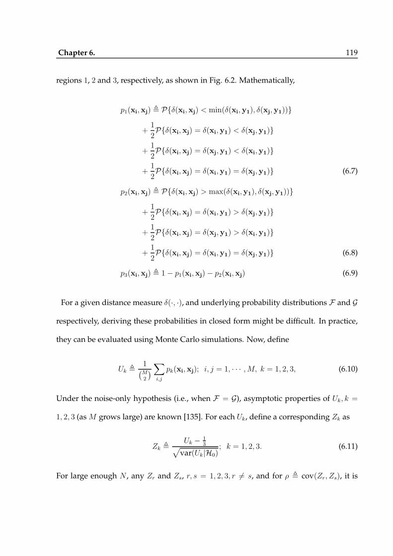
Chapter 6. 119

regions 1, 2 and 3, respectively, as shown in Fig. 6.2. Mathematically,

p1(xi,xj) , Pδ(xi,xj) < min(δ(xi,y1), δ(xj,y1))

+1

2Pδ(xi,xj) = δ(xi,y1) < δ(xj,y1)

+1

2Pδ(xi,xj) = δ(xj,y1) < δ(xi,y1)

+1

2Pδ(xi,xj) = δ(xi,y1) = δ(xj,y1) (6.7)

p2(xi,xj) , Pδ(xi,xj) > max(δ(xi,y1), δ(xj,y1))

+1

2Pδ(xi,xj) = δ(xi,y1) > δ(xj,y1)

+1

2Pδ(xi,xj) = δ(xj,y1) > δ(xi,y1)

+1

2Pδ(xi,xj) = δ(xi,y1) = δ(xj,y1) (6.8)

p3(xi,xj) , 1− p1(xi,xj)− p2(xi,xj) (6.9)

For a given distance measure δ(·, ·), and underlying probability distributions F and G

respectively, deriving these probabilities in closed form might be difficult. In practice,

they can be evaluated using Monte Carlo simulations. Now, define

Uk ,1(M2

)∑

i,j

pk(xi,xj); i, j = 1, · · · ,M, k = 1, 2, 3, (6.10)

Under the noise-only hypothesis (i.e., when F = G), asymptotic properties of Uk, k =

1, 2, 3 (asM grows large) are known [135]. For each Uk, define a corresponding Zk as

Zk ,Uk − 1

3√var(Uk|H0)

; k = 1, 2, 3. (6.11)

For large enough N , any Zr and Zs, r, s = 1, 2, 3, r 6= s, and for ρ , cov(Zr, Zs), it is

Chapter 6. 120

known that

Qr,s ,Z2r + Z2

s − 2ρZrZs1− ρ2

, r, s = 1, 2, 3; r 6= s, (6.12)

closely follows a central chi-squared distribution with 2 degrees of freedom, i.e., Qr,s ∼

χ22, under H0. This statistic can be used for testing against a given fN. Therefore, the

statistic Q , Q1,3 +Q2,3 +Q3,1 follows a central chi-square distribution with 6 degrees

of freedom. Using this result, the hypothesis testing problem (6.4), reduces to

Q≁H0

≷H0

τID. (6.13)

Since the above test statistic is constructed depending on the distance measure δ(·, ·)

between the points x1, x2, · · · , xM , it is called as the Interpoint Distance (ID) based test.

The threshold τID is chosen such that the following constraint is satisfied.

pf , Pdeclaring ≁ H0|H0 = αf , (6.14)

where αf ∈ (0, 1) is given. Under H0, since Q ∼ χ26, it is easy to see that the above

condition is satisfied when τID is chosen such that

1− γ(τID2, 3)

Γ(3)= αf , (6.15)

where γ(·, ·), and Γ(·) are lower incomplete, and complete gamma functions, respec-

tively [116].

The above test can be extended to handle the presence of class A and class B noise

components [55], as long as the distribution and their parameters are known. If the pa-

rameters are unknown, they can be directly estimated from the observations. However,

Chapter 6. 121

this test is known to perform poorly, if there is an uncertainty in the knowledge of the

noise-only distribution parameters [135].

6.3.1 Choice of δ(·, ·)

A distance function is said to be invariant under a given transformation T [135], if

δ(x1,x2) ≥ δ(x3,x4) ⇒ δ(T (x1), T (x2)) ≥ δ(T (x3), T (x4)). (6.16)

If a distance function δ(·, ·) is invariant to a transformation T (·), then the values of the

parameters Uk and ρ are not affected by T [135]. Since the relative ℓp-norm distances are

invariant to linear transformations such as scaling, rotation, etc., they are considered in

this work. As will be elaborated in Sec. 6.5, the performance of the ID detector can be

improved by appropriately choosing the parameter “p”.

6.3.2 Extension to Multiple Sensors

Oneway to extend the above analysis to the multi-sensor case (with L sensors), is to use

the sum X ,L∑l=1

Xl, as the matrix from which the test statistic is computed. Given that

every vector in each Xl is a Gaussian vector, every vector in X also follows a Gaussian

distribution. In other words, this scenario is statistically equivalent to a centralized

detector in which the fusion center has access to X1, · · · , XL, which uses X as the test

statistic. Therefore, the above procedure can now be applied on each vector of X. The

test, however, would remain the same as given in (6.13).

Chapter 6. 122

6.4 〈h, φ〉 Distance Based GoFT

Consider the scenario where L sensors transmit Rl = XlXHl to a Fusion Center (FC),

through a dedicated, lossless channel. The FC sums all the matrices Rl into a single

matrix R ,L∑l=1

Rl. Under the noise-only hypothesis, given that each Rl ∼WN (M,Σ), it

is easy to see that R ∼ WN(LM,Σ) [138].

In this section, we study the properties of 〈h, φ〉 distance metric for probability distri-

butions proposed by Salicru et al. [136], and propose a GoFT based on this metric for SS.

Let Y and Z be two positive definite, Hermitian random matrices of size N × N , with

their distributions characterized by the densities fY(·; θ1), and fZ(·; θ2), parametrized

by θ1 and θ2, respectively. Then, the 〈h, φ〉 divergence (not necessarily a distance metric,

as explained later) between fY and fZ is defined as [136]

Dhφ(Y,Z) , h

(∫

H

φ

(fY(Y

′; θ1)

fZ(Y′; θ2)

)fZ(Y

′; θ2)dY′), (6.17)

where h : [0,∞) → [0,∞) is a strictly increasing functionwith h(0) = 0, and φ : [0,∞) →

[0,∞) is a convex function, with φ(00

), 0. The space of all positive definite Hermitian

matrices of size N ×N is denoted by H. The differential element dY′ is defined as

dY′ = dY ′11dY

′22 · · · dY ′

MM

M∏

i,j=1;i<j

dRe(Y ′i,j)dIm(Y ′

i,j), (6.18)

where Y ′i,j is the (i, j)th entry of the matrixY. Also, Re(·) and Im(·) denote the real and

imaginary parts of a complex number.

Some of the well-known information-theoretic divergences are special cases of the

〈h, φ〉 divergence, with appropriate choices of h(·) and φ(·). These divergence measures

Chapter 6. 123

Table 6.1: Various information-theoretic divergences as special cases of 〈h, φ〉 distance,and their related functions h(·) and φ(·).

Divergence h(x) φ(y)

χ2 x4

(y − 1)2 y+1y

Kullback-Leibler x2

(y − 1) log y

Renyi (order α) log(αx−x+1)α−1

, 0 ≤ x ≤ 1α−1

y1−α+yα−α(y−1)−22(α−1)

, 0 < α < 1.

Bhattacharyya − log(1− x), 0 ≤ x < 1 −√y + y+1

2.

Hellinger x2, 0 ≤ x < 2 (

√y − 1)2

need not be distance measures, as they do not satisfy necessarily the triangle inequality.

A symmetric, 〈h, φ〉 distance metric based on the Dhφ divergence is defined as follows

dhφ(Y,Z) ,Dhφ(Y,Z) +Dh

φ(Z,Y)

2(6.19)

The above 〈h, φ〉 metric, viz., dhφ(·, ·) is a distance metric, i.e., it satisfies non-negativity

property, symmetric property and triangle inequalities, for all possible choices of h(·)

and φ(·), subjected to the conditioned mentioned earlier [138]. Some of the commonly

used information-theoretic divergence measures, and the corresponding h(·) and φ(·)

functions for them to be a valid Dhφ divergence, are listed in Table 6.1.

Next, we recall the following theorem ([136], [139]), which establishes the distribution

of the statistic dhφ underH0, for any h(·) and φ(·) for our problem formulation.

Theorem 9 (Salicru et al.). Let R ∼ WN (LM,Σ), and R′ be another random matrix of size

N × N . Then, under H0 (i.e., when Rd.= R′), and under the regularity conditions given by

Salicru et al. [136, Pg. 375],

S(R,R′) , LMdhφ(R,R

′)

h′(0)φ′′(1)d.−−−−→

LM→∞χ2

N2+N2

. (6.20)

Chapter 6. 124

Using the above theorem, an L sensor extension of the hypothesis testing problem in

(6.4) reduces to a test on the statistic S(R,R′), which is of the form

S(R,R′)≁H0

≷∼H0

τ (φ)

h , (6.21)

where τ (φ)

h is chosen such that the constraint pf = αf ∈ (0, 1) is satisfied. Since S(·, ·) ∼

χ2N2+N

2

, it is easy to see that the above condition is satisfied when τ (φ)

h is chosen such that

1−γ

(τ(φ)h

2, N

2+N4

)

Γ(N2+N

4

) = αf . (6.22)

Note that the above result holds for every h(·) and φ(·), such that dhφ(·, ·) is a valid

distance metric. In the next section, closed from expressions for the metric dhφ for some

of the divergence measures listed in Table 6.1 are provided.

6.4.1 Expressions for Various dhφ(·, ·)Distances

For further analysis and simulation study, we will consider the following distance met-

rics. Since themetric S(·, ·) for any dhφ(·, ·) follows the same distribution for large enough

L orM , it is sufficient to consider any one of the metrics. Later, through simulations, we

confirm that each of the following metrics give the same performance. The expressions

given in this section are special cases of the results given by Frery et al [139, Sec. 3.1].

1. The Kullback-Leibler distance (KL)

dKL(R,R′) = LM

(tr

R′−1R+R−1R′

2

−N

), (6.23)

where tr(R) represents the trace of the matrix R.

Chapter 6. 125

2. The Bhattacharyya distance (B)

dB(R,R′) = LM

2[logdet(R) + log det(R′)]− LMN log(LM)

−LM log det

[(LMR−1+LMR′−1

2

)−1], (6.24)

where det(R) represents the determinant of a matrixR.

3. The Hellinger distance (H)

dH(R,R′) = 1−

det

[(LMR−1+LMR′−1

2

)−1]

R(LM/2)R′(LM/2)

× LMLMN . (6.25)

6.4.2 Robustness of the KL Distance Metric dKL(·, ·)

In this section, we discuss a robustness feature of the Kullback-Leibler distance metric

dKL(·, ·). As observed by Frery et al. [139, Sec. 4.3], the test statistic S(R, ·) is robust

to small “contaminations” in the observations under H0, i.e., it satisfies the false-alarm

constraint under the following condition. When the matrix R under H0 is of the fol-

lowing form

Rd.= ǫWN (LM, κΣ) + (1− ǫ)WN (LM,Σ), (6.26)

where κ is a large number (∼ 1000), and 0 ≤ ǫ ≪ 1. In other words, under H0, with

probability 1 − ǫ, the noise observations come from the regular Wishart distribution,

and with probability ǫ, the observations follow a Wishart distribution, whose under-

lying Gaussian distribution has a much larger variance. The model in (6.26) is closely

related to the ǫ-mixture model, which characterizes the PDF of the background noise

Chapter 6. 126

and Middleton’s Class A model ( [55], [109], [111]), which was studied in Chap. 5.

Themain motivation for introducing theWeighted Zero-Crossings Detector (WZCD) in

Chap. 5 was the requirement of robustness of the GoFT to the presence of Class A noise

component. Therefore, the KL distance based 〈h, φ〉 detector can be seen as a solution

for robustness to the presence of Class A noise component in the multi-dimensional SS

problem setup.


As seen ealier, the performance of a GoFT for SS in a CR network needs to be studied

through extensive simulations. We consider a multiple sensor setup, with multiple

primary users with a Rayleigh fading channel from each primary transmitter to each

CR node, and is i.i.d. across space and time. For both ID and 〈h, φ〉 detectors, and in

each case, the thresholds are chosen such that the target false alarm probability is fixed

to be pf = 0.01. Unless mentioned, the distributions of primary-only observations are

modeled as Gaussian, i.i.d. across sensors. The legend entries ID, 〈h, φ〉 KL, 〈h, φ〉 B,

〈h, φ〉 H, John, ER and ST represent Interpoint distance, KL distance, Bhattacharyya

distance, Hellinger distance, John’s, eigenvalue ratio based, and sphericity test based

detectors, respectively.

6.5.1 ID Test

Figure 6.3 shows the performance of IDwith John’s, ER and ST for varying values of the

total primary average SNR, for L = 1,M = 100, N = 5, P = 2. The SNR received due

to each primary user is assumed to be equal. The distance metric was chosen to be an

Chapter 6. 127

lp norm, with p = 3. It is seen that the ID performs better than all the other techniques.

Under the same conditions, the performance of all detectors for p = 2 is shown in Fig.

6.4. In the low SNR regime, ID performs better than all the other techniques, and as

the SNR increases, ER performs slightly better. In Fig. 6.5, detection of a single PU is

considered with L = 1, M = 100, and N = 5. In this scenario, ID performs slightly

better that ER in low SNR regime, and ER performs better as SNR increases. Detection

of a single PU with L = 1, M = 80, and N = 5, as considered in Fig. 6.6 shows a

different trend where ER performs better that ID. However, ID performs better that

both John and ST detectors.

−10 −9 −8 −7 −6 −50

0.1

0.2

0.3

0.4

0.5

0.6

0.7

0.8

Primary SNR (dB)

Pro

bab

ilit

y o

f dec

lari

ng "

not

H0"

ID

John

ER

ST

Figure 6.3: Performance comparison of detection of primary under Rayleigh fading,with L = 1,M = 100, N = 5, P = 2, and p = 3.

Chapter 6. 128

−10 −8 −6 −4 −2 00

0.2

0.4

0.6

0.8

1

Primary SNR (dB)

Pro

bab

ilit

y o

f dec

lari

ng "

not

H0"

ID

John

ER

ST


6.5.2 〈h, φ〉 Test

Figure 6.7 shows the performance comparison of the Kullback Liebler (KL) and Bhat-

tacharyya (B) based 〈h, φ〉 detectors with the ER, John and ST detectors, with respect

to the total primary SNR, for L = 10, M = 200, N = 4 and P = 3. As expected, the

performances of KL and B detectors are nearly equal. As the SNR increases, a huge per-

formance improvement is observed in using the 〈h, φ〉 detectors, as compared to other

techniques. Similar trends are observed in Fig. 6.8, where the parameters are chosen

to be L = 10, M = 200, N = 4 and P = 5. Since the presence of an extra PU increases

the detection SNR, performance improvements are seen in Fig. 6.8, as compared to Fig.

6.7. In Fig. 6.9, where the parameters are L = 10, M = 50, N = 5 and P = 4, it is

seen that as the SNR increases, improvements in the performances of all the detectors

are seen. However, even in this case, the 〈h, φ〉 based detectors perform better than the

Chapter 6. 129

−10 −8 −6 −4 −2 00

0.2

0.4

0.6

0.8

1

Primary SNR (dB)

Pro

bab

ilit

y o

f dec

lari

ng "

not

H0"

ID

John

ER

ST


others. Similar trends are carried over in Fig. 6.10, with L = 10, M = 50, N = 5 and

P = 5. As seen earlier, a performance improvement in all the detectors are seen due to

the presence of extra PUs. Finally, Fig. 6.11 shows the performance curves of the all the

〈h, φ〉 detectors studied in Sec. 6.4.1. As expected, the performance of all the detectors

are nearly the same, across different values of P .

6.6 Conclusions

In this chapter, we studied two multi-dimensional Goodness-of-Fit tests for spectrum

sensing in cognitive radios. Both the tests, viz., the Interpoint Distance (ID) based test

and the 〈h, φ〉 distance based tests were constructed based on the properties of stochas-

tic distances. The construction of the ID test was studied for a single CR node case with

multiple antenna, multiple observations from multiple primary users. The 〈h, φ〉 test

Chapter 6. 130

−10 −8 −6 −4 −2 00

0.2

0.4

0.6

0.8

1

Primary SNR (dB)

Pro

bab

ilit

y o

f dec

lari

ng "

not

H0"

ID

John

ER

ST


was studied for the multiple CR nodes. Also, a robustness feature of the KL distance

based test was studied, which has connections with Middleton’s Class A noise model.

The proposed tests were shown to perform better that the existing techniques such as

the eigenvalue ratio based test, John’s test, and the sphericity test, in several scenarios.

Chapter 6. 131

−12 −11 −10 −9 −8 −70

0.2

0.4

0.6

0.8

1

Primary SNR (dB)

Pro

bab

ilit

y o

f dec

lari

ng "

not

H0"

<h,φ> KL

<h,φ> B

John

ER

ST

Figure 6.7: Performance comparison of detection of primary under Rayleigh fading,with L = 10,M = 200, N = 4, P = 3.

−12 −11 −10 −9 −8 −70

0.2

0.4

0.6

0.8

1

Primary SNR (dB)

Pro

bab

ilit

y o

f dec

lari

ng "

not

H0"

<h,φ> KL

<h,φ> B

John

ER

ST


Chapter 6. 132

−10 −8 −6 −4 −2 00

0.2

0.4

0.6

0.8

1

Primary SNR (dB)

Pro

bab

ilit

y o

f det

ecti

on

<h,φ> KL

<h,φ> B

John

ER

ST


−10 −8 −6 −4 −2 00

0.2

0.4

0.6

0.8

1

Primary SNR (dB)

Pro

bab

ilit

y o

f dec

lari

ng "

not

H0"

<h,φ> KL

<h,φ> B

John

ER

ST


Chapter 6. 133

−6 −5.5 −5 −4.5 −4 −3.50

0.2

0.4

0.6

0.8

1

Primary SNR (dB)

Pro

bab

ilit

y o

f dec

lari

ng "

not

H0"

<h,φ> KL

<h,φ> H

<h,φ> B

P=5

P=3

P=4

P=1

P=2

Figure 6.11: Performance comparison of detection of primary under Rayleigh fading,with L = 20,M = 15, N = 1.

Chapter 7

Conclusions and Future Work

In this thesis, we investigated the problem of spectrum sensing in cognitive radios. The

main contributions of this thesis are summarized below.

7.1 Contributions

In chapter 2, we analyzed the performance of energy-based Bayesian decentralized de-

tection for spectrum sensing in cognitive radios. We showed that, for various fading

models, with the OR rule for decision fusion, the conventional error exponent is equal

to zero. We introduced a novel performance metric called the Error Exponent with a

Confidence Level (EECL), and showed that the EECL at a given confidence level q < 1

is strictly positive. We used the EECL to answer the question of whether it is better to

sense for the pilot tone in a narrow band, or to sense the entire wide-band signal. We

also derived simplified expressions for finding the detection threshold and the EECL

for the i.i.d. Rayleigh fading and lognormal shadowing cases. We validated the theo-

retical expressions through Monte Carlo simulations.

Chapter 3 considered the problem of Bayesian decentralized SS in CR networks under

134

Chapter 7. 135

various fading environments. A CLT-based approximation was explored, which led to

analytical expressions for near-optimal detection thresholds for Rayleigh, Lognormal,

Nakagami-m, Weibull fading cases. For the Suzuki fading case, a generalized gamma

approximation was provided, which saves on the computation of an integral. Also,

in the Rayleigh fading case, a structural property of the detector, viz., the trade-off

between M and P to maintain a given pe at the individual sensors, in the low SNR

regime, was discussed. Extending to the decentralized case withN sensors, the optimal

exponent on PE was derived in closed form. The accuracy of the theoretical expressions

and the diversity gain obtainable through the use ofN sensors were illustrated through

simulations.

In chapter 4, we considered the problem of spectrum sensing in the presence of a

multiuser frequency-hopping primary network. We theoretically analyzed the perfor-

mance of the FAR algorithm, and validated the results through simulations. We de-

rived the sensing duration that maximizes the throughput of the CR system, under a

constraint on the interference to the primary network. We also presented a technique

to synchronize the CR system with the primary hopping instants. The FAR algorithm

was implemented on Lyrtech SFF SDR DP and its performance corroborated well with

the ROCs obtained from Monte Carlo simulations.

In chapter 5, a weighted zero-crossings based goodness-of-fit test for spectrum sens-

ing was proposed. A near-optimal detection threshold was derived for the specific

choices of uniform and exponential weights. It was shown that this detector is robust

to uncertainties in the noise model and parameters. Through simulations, it was shown

Chapter 7. 136

that the proposed detectors outperform the existing tests in the CR literature in a vari-

ety of noise and primary signal conditions of practical interest. Also, the computational

simplicity of the proposed test was highlighted. Therefore, the proposed detector is a

promising choice for spectrum sensing in CR, and can be used in a wide range of com-

munication scenarios.

Finally, in chapter 6, we studied twomulti-dimensional Goodness-of-Fit tests for spec-

trum sensing in cognitive radios. Both the tests, viz., the Interpoint Distance (ID) based

test and the 〈h, φ〉 distance based tests were constructed based on the properties of

stochastic distances. The construction of the ID test was studied for a single CR node

case with multiple antenna, multiple observations from multiple primary users. The

〈h, φ〉 test was studied for the multiple CR nodes. Also, a robustness feature of the KL

distance based test was studied, which has connections with Middleton’s Class A noise

model. The proposed tests were shown to perform better that the existing techniques

such as the eigenvalue ratio based test, John’s test, and the sphericity test, in several

scenarios.

7.2 Future Work

Future work for spectrum sensing in cognitive radios could include the following is-

sues. Some of them are already being addressed by the author.

• For the Bayesian decentralized detection, incorporating correlation in the signal

or noise, extending the results to allow for time-varying channels, and optimally

combining the outcomes from NB andWB spectrum sensing, could be interesting

extensions.

Chapter 7. 137

• In Bayesian SS, the low-rate channel between the individual sensors and the FC

was assumed to be lossless. Design and analysis of decentralized SS accounting

for the effect of fading and noise in this channel would be useful under practical

scenarios.

• For the detection of frequency-hopping primary signals, there exists a tradeoff:

depending on the total number of available bands, active primary and secondary

users, a CR can either continue to sense for a channel throughout the sensing du-

ration, or to jump into another possibly vacant channel and perform fresh sensing.

This exploration-exploitation tradeoff is challenging, and could lead to interesting

results.

• The WZCD, or in general, any CFAR detector was found to fail when the pri-

mary signal also follows another Gaussian distribution with a different variance.

Given the advantages of the WZCD, modifying the Ψ2M statistic or proposing a

new detector based on the statistics of zero-crossings to incorporate detection of

the Gaussian signals could make the GoFT stronger.

• In general, spectrum sensing under an energy efficiency constraint have not been

dealt in greater detail in the literature so far. Given the importance of green com-

munications, such a study could lead to important designs that consume less en-

ergy and yet offer good performance.

Appendix A

Appendix for Chapter 2

A.1 Proof of Theorem 1

It is straightforward to show that, under Rayleigh fading, the likelihood ratio test cor-

responding to (2.1) is monotonically increasing in Vy, and hence, the optimum test re-

duces to a threshold test on Vy itself. That is, it declares H1 when Vy ≥ x, where x is the

detection threshold. Let fα(α) denote the pdf of α. Conditioned on A , α ≥ α0, the

pdf of α is fα|A(α|A) = fα(α)/P(A), α ≥ α0. By construction, P(A) = q. The probability

of error is given by

pe = π0Q(x√M) + π1

x∫

−∞

∞∫

α0

fN

(v − αP,

1√M

)fα(α)

qdαdv, (A.1)

where fN (x, σ) is the Gaussian pdf with mean zero and variance σ2 evaluated at x,

π0 , P(H0), and π1 , P(H1) = 1− π0. To find the optimum threshold, we differentiate

the above w.r.t. x and equate to 0. After some simplification, we get

qπ0π1

=

∞∫

α0

exp

(M

(xαP − α2P 2

2

))fα(α)dα. (A.2)

138

Appendix A. 139

Let xM denote the solution to the above equation for a given value of M .1 First, we

show that xM converges to α0P/2. To do this, we show that neither xM < α0P/2 nor

xM > α0P/2 are possible for largeM , as they lead to a contradiction. Define g(x, α) ,

xαP − α2P 2/2. Note that g(α0P/2, α) ≤ 0 for α ≥ α0. If xM < α0P/2, since g(x, α) is

monotonic in x, we have g(xM , α) < 0 for α ≥ α0. Let gmax , maxα≥α0 g(xM , α), and

note that gmax < 0. Then, using gmax ≥ g(xM , α) in (A.2) results in the following upper

bound on the right hand side (RHS): RHS ≤ exp(Mgmax)∫∞α0fα(α)dα. Since gmax < 0,

the upper bound can be made as small as desired by choosing M sufficiently large.

Thus, if xM < α0P/2, the right hand side goes to zero as M gets large, and hence,

attaining equality in (A.2) is not possible. Hence, xM must satisfy xM ≥ α0P/2.

Next, we show that xM ≥ x0 > α0P/2 also leads to a contradiction. Consider α

such that g(x0, α) > 0. This corresponds to α < 2x0/P . By the assumption, we have

α0 < 2x0/P , so that, g(x0, α) > 0 for α0 ≤ α < 2x0/P . Further, if g(x0, α) > 0 and

xM ≥ x0, we have g(xM , α) > 0. Therefore, there exists an ǫ > 0 such that g(xM , α) > 0

for α0 ≤ α ≤ 2x0/P − ǫ. Let gmin , minα∈[α0,2x0/P−ǫ] g(xM , α), and note that gmin > 0.

Then, the right hand side in (A.2) can be lower bounded as

RHS ≥∫ 2x0

P−ǫ

α0

exp (Mg(xM , α)) fα(α)dα (A.3)

≥ exp (Mgmin)

∫ 2x0P

−ǫ

α0

fα(α)dα. (A.4)

Since gmin > 0, the above lower bound can be made as large as desired by choosing M

sufficiently large, since the integral term is a strictly positive constant. This implies that

if xM ≥ x0 > α0P/2, the right hand side grows unbounded asM gets large, and hence,

1That a unique solution exists can be seen from simple monotonicity arguments.

Appendix A. 140

attaining equality in (A.2) is not possible. Hence, xM converges to α0P/2 asM goes to

infinity.

Now, consider the exponent due to the false alarm term. This is simply given by

ǫf , limM→∞

− log(Q(xM

√M))

M=α20P

2

8. (A.5)

In the above, Q(y) is the standard Gaussian tail probability evaluated at y. The second

equality above is obtained by upper and lower bounding Q(y) for large y and showing

that both limits equal as M → ∞. Since the exponents due to the false alarm and the

missed detection are equal in a Bayesian set-up [48, Chap. 11], [71], it follows that the

EECL(q) on the probability of error isα20P

2

8, where α0 is chosen to satisfy P(α > α0) = q.


Suppose that the hypothesis H0 is true. With the OR fusion rule, a false alarm at any of

the sensors results in a false alarm at the FC. Since, conditioned on H0, the sensor deci-

sions are independent, the false alarm probability at the FC, denoted by PF , is simply

1−(1−pf)N , where pf is the false alarm probability at an individual sensor. Now, given

the detection threshold α0P2

at the sensors, the exponent ǫF at the FC is determined by

the pf term in the expansion of 1 − (1 − pf )N . Thus, the error exponent at the FC is the

same as that at the individual sensors, i.e., ǫF = (α0P )2

8.

Suppose that the hypothesis H1 is true. Conditioned on αj , the channel power gain

from the primary transmitter to sensor j, the decision statistic Vy at the jth sensor is

Appendix A. 141

distributed asN(αjP,

1M

). Since the jth sensor uses a threshold of α0P

2for detection, us-

ing well-known bounds on the Q-function,2 it is easy to show that the missed detection

probability at the jth sensor conditioned on αj , denoted pmj |αj, is given by

pmj |αj= P

Vy <

α0P

2

∣∣∣∣αj

= Q

(√M

(α0P

2− αjP

)).= exp

(−M

2

(αjP − α0P

2

)2

Iαj>α02

)(A.6)

where the notation f(M).= exp(−Mβ) is used to mean limM→∞

− log f(M)M

= β. That

is, the jth sensor achieves an error exponent of 12

(αjP − α0P

2

)2if αj >

α0P2, and zero

otherwise.

With the OR fusion rule, when hypothesis H1 is true, the FC makes an error and

declares H0 only if all the sensors make an error. Hence, given α1, · · · , αN , the missed

detection probability at the FC PM |α1,··· ,αNis given by

PM |α1,··· ,αN=

N∏

j=1

pmj

.= exp

(−M

2

N∑

j=1

(αjP − α0P

2

)2

Iαj>α02

). (A.7)

Now consider the case where α1, α2, . . . , αN are random. The FC attains an EECL(q)

of ǫM , provided

P1

2

N∑

j=1

(αjP − α0P

2

)2

Iαj>α02 ≤ ǫM

≤ 1− q, (A.8)

where the probability is taken over the distribution of α1, α2, . . . , αN . The best error

exponent is obtained, i.e., ǫM is maximized, when the left hand side above equals 1− q,

since, otherwise, ǫM (and α0) can be increased to improve the error exponent.

2For example, y

1+y2

1√

2πe−

y2

2 ≤ Q(y) ≤ 1

y√

2πe−

y2

2 .

Appendix A. 142

Finally, for optimal Bayesian detection, the exponent associated with the false alarm

and missed detection must be equal, i.e., ǫF = ǫM [48, Chap. 11], [71]. Hence, substitut-

ing ǫM = (α0P )2

8in (A.8) and simplifying, we get (2.2), which completes the proof.

A.3 Proof of Corollary 1

Let α0 and ℓ0 denote the solution to (2.2) under the Rayleigh fading and lognormal

shadowing cases, respectively. Let expn(λ) and LN(µ, σ) denote the exponential dis-

tribution with parameter λ and the lognormal distribution with parameters µ and σ,

respectively. Now, under Rayleigh fading, tj ,2αj

α0∼ expn

(2α0

), while under lognor-

mal shadowing, with a slight abuse of notation, tj ,2αj

ℓ0∼ LN

(µs + log

(2ℓ0

), σs

). For

notational convenience, let Z ,∑N

j=1 (tj − 1)2 I(tj−1)≥0. From Theorem 2, note that we

need to find α0 such that FZ(1) = 1− q, where FZ(·) is the CDF of Z.

PZ ≤ 1 =N∑

l=0

Pl out of N tj ’s are ≥ 1PZ ≤ 1|l out of N tj’s are ≥ 1(A.9)

=

N∑

l=1

(N

l

)(P tj ≤ 1)N−l(P tj > 1)l

P

l∑

k=1

(tk − 1)2 ≤ 1

∣∣∣∣∣ tk > 1, k = 1, . . . , l

+ (P tk ≤ 1)N ,

which should equal 1 − q by requirement. For Rayleigh and shadowing caess, tk ∼

expn

(2α0

)and tk ∼ LN

(µs + log

(2ℓ0

), σs

), respectively. In the Rayleigh fading case, by

the memoryless property of exponential random variables, it is easy to show that

P

l∑

k=1

(tk − 1)2 ≤ 1

∣∣∣∣∣ tk > 1, k = 1, . . . , l

= P

l∑

k=1

a2k ≤ 1

, (A.10)

Appendix A. 143

where ak ∼ expn

(2α0

)are independent and exponentially distributed. Since P tk > 1

= e− 2

α0 , (A.10) reduces to the expression in (2.3).

The proof for the lognormal shadowing case is similar to the Rayleigh fading case,

and follows by noting that P tk ≤ 1 = P log tk ≤ 0 = Q

(µs+log

(

2ℓ0

)

σs

). Further,

P

l∑

k=1

(tk − 1)2 ≤ 1

∣∣∣∣∣ tk > 1, k = 1, . . . , l

= P

l∑

k=1

(eyk − 1)2 ≤ 1

. (A.11)

In the above, yk , log tk, and, due to the conditioning on tk > 1, we have that yk has a

truncated Gaussian distribution, with pdfN(

µs+log(

2ℓ0

)

,σ2s

)

Q

(

−µs+log( 2

ℓ0)

σs

) for yk > 0 and zero otherwise.

A.4 Proof of Corollary 2

Consider the left hand side of (2.3). Upper bounding the terms in the expression would

lead to a lower bound on α0, and, consequently, on the EECL(q). First, note that 1 −

exp(α0

2

)≤ α0

2. Also, ak in (2.3) is distributed as fak(ak) = α0

2exp

(−α0ak

2

), ak ≥ 0, and

hence, fak(ak) ≤ α0

2. Thus, by replacing the pdf of ak with its upper bound, we get

P(

l∑

k=1

a2k ≤ 1

)=

∫∑l

k=1 a2k≤1,ak≥0

fak(a1)fak(a2) · · ·fak(al)da1da2 · · ·dal

≤(α0

2

)l ∫∑l

k=1 a2k≤1,ak≥0

da1da2 · · ·dal =(α0

2

)l Vl2l, (A.12)

where Vl = πk2

Γ(1+ k2 )

is the volume of the l-dimensional unit sphere, with Γ(·) being the

Gamma function. The 2l factor in the denominator arises because only the volume of

the first orthant is relevant here, since ak ≥ 0. Substituting in (2.3), we get a lower

Appendix A. 144

bound on α0 by solving

(αLB02

)N+

N∑

l=1

(N

l

)(αLB02

)N−l(αLB02

)l Vl2l

= 1− q. (A.13)

The result in (2.6) follows from rearranging the above equation.

The proof for the lognormal shadowing case is similar. Starting from (2.4), using a

well-known bound on the Q-function, we upper bound PA as

PA ≤ 1√2π

exp

−

(log(

2ℓ0

))2

2σ2s

. (A.14)

Next, conditioned on yk > 0, it is easy to show that zk , eyk − 1 is distributed as

fzk(zk) =1

(zk + 1)σs√2π

exp(− (log(zk+1)−log(2/ℓ0))

2

2σ2s

)

Q(

− log(2/ℓ0)σs

) , zk ≥ 0. (A.15)

Further, since ℓ0 ≤ 1, setting zk = 0 in the right hand side above leads to an upper

bound on fzk(zk). Hence, we have

P(

l∑

k=1

z2k ≤ 1

)≤

1

σs√2π

exp(− (log(2/ℓ0))

2

2σ2s

)

Q(− log(2/ℓ0)

σs

)

l

Vl2l. (A.16)

Substituting the upper bounds in (A.14) and (A.16) into (2.4), and using the fact that

PAc = Q(− log(2/ℓ0)

σs

), and simplifying, we get the result in (2.7).

Appendix A. 145


It is known that, with conditionally i.i.d. observations at the sensors, the probability of

error at the FC is minimized by theK out ofN rule, and the optimumK is given by [84]

Kopt = min

N,

log(

π01−π0

)+N log

(1−pfpm

)

log(

1−pmpf

)(1−pfpm

)

, (A.17)

where pf and pm are the false alarm and missed detection probabilities, respectively,

at the individual nodes. Now, given the detection threshold α0P2

> 0 at the individual

sensors, pf clearly decreases with an exponent (α0P )2

8. On the other hand, whenever

α < α0, the missed detection probability of the hypothesis test in (2.1) is lower bounded

by 12. Since the event α < α0 occurs with a nonzero probability, the exponent on pm is 0.

Thus,

log(

π01−π0

)+N log

(1−pfpm

)

log(

1−pmpf

)(1−pfpm

)

→ 1, (A.18)

since the numerator approaches a constant, while the denominator is linearly increas-

ing withM . Thus, for sufficiently largeM , Kopt = 1, i.e., the OR fusion rule is optimal.

A.6 Expressions for Approximations in Sec. 2.4, Cor. 1

A.6.1 Weibull Sum Approximation in Rayleigh Fading Case

Consider the probability term in (2.3), viz., P∑l

k=1 a2k

≤ 1, where ak is a exponen-

tially distributed random variable with parameter 2α0. Following the genesis [116], a

random variable X is said to be Weibull distributed with shape and scale parameters

aw and bw, respectively, if(Xbw

)awis a standard exponential random variable. Using this

result, it is easy to see that a2k follows a Weibull distribution with parameters aw = 0.5,

Appendix A. 146

and bw = α0/2.

Now, following [85], the PDF and CDF of the term Al ,∑l

k=1 a2k can be tightly ap-

proximated by a α− µ distribution, whose expressions are given by

fAl(a) =

αµµaαµ−1

ΩµΓ(µ)exp

(−µa

α

Ω

); and FAl

(a) =γinc

(µ, µa

α

Ω

)

Γ(µ), (A.19)

where γinc(·, ·) is the lower incomplete gamma function.

Using the following equations give moment based estimators for α, µ and Ω.

Γ2(µ+ 1

α

)

Γ(µ)Γ(µ+ 2

α

)− Γ2

(µ+ 1

α

) =E2Al

EA2l − E2Al

Γ2(µ+ 2

α

)

Γ(µ)Γ(µ+ 4

α

)− Γ2

(µ+ 2

α

) =E2A2

l

EA4l − E2A2

l

Ω =

[µ1/αΓ(µ)EAl

Γ(µ+ 1

α

)]α. (A.20)

The expectation terms can be found out by using multinomial expansion as

EAnl =n∑

n1=0

n1∑

n2=0

· · ·nl−2∑

nl−1=0

(n

n1

)(n1

n2

)· · ·(nl−2

nl−1

)Ean−n1

1 Ean1−n22 · · ·Eanl−1

l ,with

Eank = bn/aww Γ

(1 +

n

aw

), (A.21)

for any positive integer n.

The above approximation has been found to be very tight [85], and is applicable for

all values of aw > 0, unlike other exact expressions or approximations available in the

literature. For e.g., Yilmaz and Alouini [140] have derived the exact PDF of Weibull

sums, but are applicable only when aw > 1.

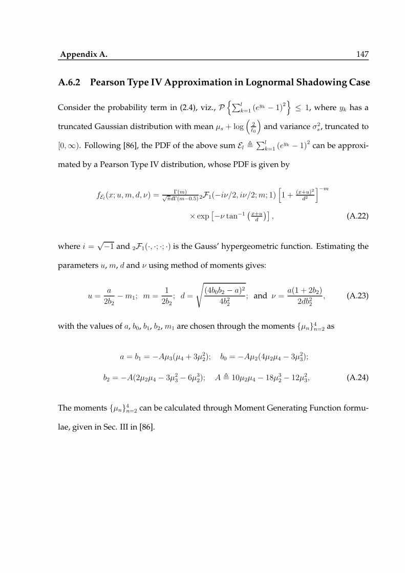
Appendix A. 147

A.6.2 Pearson Type IVApproximation in Lognormal ShadowingCase

Consider the probability term in (2.4), viz., P∑l

k=1 (eyk − 1)2

≤ 1, where yk has a

truncated Gaussian distribution with mean µs + log(

2ℓ0

)and variance σ2

s , truncated to

[0,∞). Following [86], the PDF of the above sum El ,∑l

k=1 (eyk − 1)2 can be approxi-

mated by a Pearson Type IV distribution, whose PDF is given by

fEl(x; u,m, d, ν) =Γ(m)√

πdΓ(m−0.5) 2F1(−iν/2, iν/2;m; 1)

[1 + (x+u)2

d2

]−m

× exp[−ν tan−1

(x+ud

)], (A.22)

where i =√−1 and 2F1(·, ·; ·; ·) is the Gauss’ hypergeometric function. Estimating the

parameters u,m, d and ν using method of moments gives:

u =a

2b2−m1; m =

1

2b2; d =

√(4b0b2 − a)2

4b22; and ν =

a(1 + 2b2)

2db22, (A.23)

with the values of a, b0, b1, b2,m1 are chosen through the moments µn4n=2 as

a = b1 = −Aµ3(µ4 + 3µ22); b0 = −Aµ2(4µ2µ4 − 3µ2

3);

b2 = −A(2µ2µ4 − 3µ23 − 6µ3

2); A , 10µ2µ4 − 18µ32 − 12µ2

3, (A.24)

The moments µn4n=2 can be calculated through Moment Generating Function formu-

lae, given in Sec. III in [86].

Appendix B


B.1 Proof of Theorem 4

Since the test is of the form (3.4), the optimal threshold can be found by differentiating

the probability of error with respect to the threshold, and equating it to zero. Following

(3.3) and (3.7), a straightforward substitution and simplification of the LR test results in

the expression for pe under Rayleigh fading for the problem in (3.1) as

pe = π0P(Vy > x|H0) + (1− π0)P(Vy ≤ x|H1)

= π0Q(√

Mx)+ (1− π0)

∫∞0 Q

(−x−αP

1√M

)e−αdα (B.1)

In the above equation, α , |h|2 has the exponential distribution, and x is the detection

threshold. The x(R)CLT which minimizes (B.1) can be obtained by equating ∂pe∂x

to zero,

which gives

∂pe∂x

= −π0√M

2πexp

(−Mx2

2

)+

(1− π0)

Pexp

(−Mx2

2

)exp

((x− 1

MP

)2

2/M

)

×Q

(−(x− 1

MP

)

1/√M

)= 0. (B.2)

148

Appendix B. 149

SinceM is assumed to be sufficiently high, using the approximation Q(y) ≈ exp(−y2

2),

and further simplification gives the required result.


For small values of P , using Result 1, the lognormal distribution can be approximated

by N (P, P 2σ2s). Let s , |h|2. Using this, the PDF under H1, denoted by P (Vy|H1) is

shown to be

P (Vy|H1) =

∫ ∞

0

Q

(−Vy − sP

1√M

)1

s√

2πσ2s

exp

(−(log s− logP )2

2σ2s

)ds (B.3)

≈∫ ∞

0

Q

(−Vy − sP

1√M

)1√

2πP 2σ2s

exp

(−(s− P )2

2P 2σ2s

)ds (B.4)

=1

2π√

P 2σ2sM

exp

(− V 2

y

2/M− 1

2σ2s

)

×∫ ∞

0

exp

(−[M

2+

1

2P 2σ2s

]s2 +

[Vy1/M

+1

Pσ2s

])ds. (B.5)

The above integral has a closed form solution [116, Pg. 336, eq. 3.322(1)]. Following this

result,

∫ ∞

0

exp

(−[M

2+

1

2P 2σ2s

]s2 +

[Vy1/M

+1

Pσ2s

]s

)ds =

√π

4(M2+ 1

2P 2σ2s

)

× exp

[Vy1/M

+ 1Pσ2s

]2

4(M2+ 1

2P 2σ2s

)

1− erf

[Vy1/M

+ 1Pσ2s

]

2

√(M2+ 1

2P 2σ2s

)

(B.6)

Using the above result and (3.3), the likelihood ratio can be written as

Appendix B. 150

LR(Vy) =2√

2π P2σ2sM

exp

(− 1

2σ2s

)√π

4(M2+ 1

2P 2σ2s

)

× exp

[Vy1/M

+ 1Pσ2s

]2

4(M2+ 1

2P 2σ2s

)

Q

−

(Vy1/M

+ 1Pσ2s

)

√2(M2+ 1

2P 2σ2s

)

where, we have used the result 1− erf(y) = 2Q(√2y).

The LR(Vy) can be shown to be monotone in Vy, by examining the derivative to be

positive ∀ Vy. The corresponding mathematical expressions are lengthy and therefore

omitted. Hence, the test can be written in terms of Vy, as in (3.4). Writing out the

derivative of the missed detection probability pm, and by using (B.6), it can be shown

that

∂pm∂x

=1

π√

P 2σ2sM

exp

(− x2

2/M− 1

2σ2s

)√π

4(M2+ 1

2P 2σ2s

)

× exp

[x

1/M+ 1

Pσ2s

]2

4(M2+ 1

2P 2σ2s

)

Q

−

x1/M

+ 1Pσ2s√

2(M2+ 1

2P 2σ2s

)

.

Upon equating ∂pe∂x

= π0

∂pf∂x

+ (1− π0)∂pm∂x

= 0, and further simplification gives

Kc exp

(ρ2

2

)Q(−ρ) = π0

1− π0, (B.7)

where Kc is defined as in (3.13) and ρ ,Mx+ 1

Pσ2s

√

(

M+ 1

P2σ2s

)

. For high M and low σ2s , we use

the approximation exp(ρ2

2

)Q(−ρ) ≈ exp

(ρ2

2

)− 1. Rearranging the terms gives the

required result.

Appendix B. 151


Let ζ , |h|2. Following (3.2), the likelihood ratio LR(Vy) (upon expanding and com-

pleting the squares on the exponential term) can be written as

LR(Vy) =KK

PKΓ(K)exp

((Vy − K

MP

)2

2/M

)∫ ∞

0

ζK−1e

(

−M2 (ζ−Vy+

KMP )

2)

dζ. (B.8)

The integral term∫∞0(·) in the above equation can be written as a difference between

two integrals∫∞−∞(·) and

∫ 0

−∞(·). The first integral is known to be equal to [141, Sec. III,

eq. (11) and (12)]

∫ ∞

−∞ζK−1 exp

(−M

2

(ζ−Vy+

1

MP

)2)dζ

=

(1

M

)K−12

√2π

M

[i√2 sign

(Vy−

K

MP

)]K−1

U(−K − 1

2;1

2;−(Vy− K

MP

)2

2/M

)(B.9)

=

(2M

)K−12

Γ(K2 )√πM(−K−1

2; 12;−(Vy− K

MP )2

2/M

), K odd.

2K2

(1M

)K−22(Vy− K

MP

) Γ(K+12 )√π

M(−2−K

2; 32;−(Vy− K

MP )2

2/M

), K even.

(B.10)

where, i =√−1, U(·; ·; ·) and M(·; ·; ·) are the Tricomi’s, and Kummer’s confluent

hypergeometric functions; also called as the hypergeometric function of the second,

and first kind, respectively [116]. We can use either (B.9) or (B.10) to solve the above

integral. For convenience, we will use (B.9).

Now, the second integral represents the (K − 1)th partial moment of a Gaussian ran-

dom variable, and is derived in Winkler et al. [142]. Let X ∼ N (µ, σ2). Then, let the

nth-ordered partial moment be defined as

Ez−∞(Xn) ,

∫ z

−∞xn√M

2πexp

(−(Vy − K

MP

)2

2/M

), (B.11)

Appendix B. 152

and let X∗ represent the standard Gaussian corresponding to X . In our problem, we

have X ∼ N(Vy − K

MP, 1M

), and we can write [142, Sec. 2]

∫ 0

−∞ζK−1 exp

(−(ζ − Vy +

1MP

)2

2/M

)dζ =

K−1∑

k=0

(K − 1

k

)

(Vy −

1

MP

)k (1

M

)K−1−k2

E−M(Vy− K

MP )−∞

(XK−1−k

∗)

(B.12)

where,

E−M(Vy− K

MP )−∞

(XK−1−k

∗),A

−M(Vy− KMP )

K−1−k√2π

exp

(−(Vy − K

MP

)2

2/M

)

+B−M(Vy− K

MP )K−1−k Q

(−(vy − K

MP

)√

1/M

), (B.13)

with Q(·) being the Gaussian-Q function, and

A−M(Vy− K

MP )K ,

−(−(Vy− K

MP )√1/M

)K−1

−K−1

2∑q=1

[q∏r=1

(K − 2r + 1)

](−(Vy− K

MP )√1/M

)K−1−2q, K odd.

−(−(Vy− K

MP )√1/M

)K−1

−K−2

2∑q=1

[q∏r=1

(K − 2r + 1)

](−(Vy− K

MP )√1/M

)K−1−2q, K even.

(B.14)

B−M(Vy− K

MP )K ,

0, K odd.K2∏r=1

(K − 2j + 1), K even.(B.15)

Substituting the above expression in (B.8), we get

LR(Vy) =KK

PKΓ(K)exp

((Vy − K

MP

)2

2/M

)(1

M

)K−12

√2π

M[i√2 sign

(Vy−

K

MP

)]K−1

U(−K − 1

2;1

2;−(Vy− K

MP

)2

2/M

)

−K−1∑

k=0

(K−1

k

)(Vy−

K

MP

)k(1

M

)K−1−k2

E−M(Vy− K

MP )−∞

(XK−1−k

∗)

(B.16)

Appendix B. 153

The ED is an optimal test when LR(Vy) is monotone in Vy, so that it can be written as a

test on Vy. The function U(·; ·; ·) can be represented as a (K−1)th order polynomial in Vy.

Therefore, the above function LR(Vy) need not bemonotone in Vy. Hence, in general, no

conclusion on the optimality of a test of the form (3.4), under Nakagami-m fading can

be drawn. Note that the parameter of the Nakagami-m distribution viz., K, signifies

the “number of paths” in a multipath fading environment. In an earlier result [143], the

authors have shown that the ED for detection using an equal gain combining receiver

when the channel undergoes Rayleigh fading, is only locally optimal. The structure of a

K-fold equal gain combining receiver under Rayleigh fading is statistically equivalent

to a single receiver with Nakagami-K fading. Therefore, the ED is not optimal for

detection under Nakagami-m fading channel.

In the following, we show that the ED, or a test of the form (3.4) is a Locally Most

Powerful (LMP) test [44] around x = KMP

. In the analysis of the Rayleigh fading case

(which is a special case of this problem with K = 1), it was seen that the optimal

threshold was around 1MP

, as shown in (3.8). Intuitively, for the Nakagami-m case with

parameter K, we expect that x(Nm)CLT will be in and around K

MP. Writing out pf and pm

from (3.5) and (3.6), respectively, following a similar approach used in deriving LR(Vy),

and equating ∂pe∂x

= 0, gives

π0

√M

2πexp

(−MV 2

y

2

)+ (1− π0)

√M

2π

KK

PKΓ(K)exp

(−MV 2

y

2+

(Vy− K

MP

)2

2/M

)

(1

M

)K−12

√2π

M

[i√2 sign

(Vy−

K

MP

)]K−1

U(−K − 1

2;1

2;−(Vy− K

MP

)2

2/M

)

−K−1∑

k=0

(K−1

k

)(Vy−

K

MP

)k(1

M

)K−1−k2

E−M(Vy− K

MP )−∞

(XK−1−k

∗)

= 0. (B.17)

Appendix B. 154

Using the Taylor series expansion on the Tricomi confluent hypergeometric function

U (a; b; z) around z = 0 gives [116]

U(K − 1

2;1

2;−(x− K

MP

)2

2/M

)≈ Γ(1/2)

Γ(1− K

2

) +(x− K

MP

)2

2/M× (K − 1)Γ(1/2)

Γ(1− K

2

)

− i

(x− K

MP

)√

2/M× Γ(−1/2)

Γ(−K−1

2

) , (B.18)

where i =√−1. Considering the last term of the integral in (B.12), we can approximate,

E−M(x− K

MP )−∞

(XK−1−k

∗)≈(Vy −

K

MP

)K−1

Q

(−√M

(Vy −

K

MP

)), ∀k (B.19)

By using (B.19) and (B.18), LR(Vy) is given by,

LR(Vy) ≈KK

PKΓ(K)exp

((Vy − K

MP

)2

2/M

)(1

M

)K−12

[[i√2 sign

(Vy −

K

MP

)]K−1√

2π

M

×

Γ(1/2)

Γ(1− K

2

) +(K−1)Γ(1/2)Γ(1− K

2

) ×(Vy− K

MP

)2

2/M− i

Γ(−1/2)

Γ(−K−1

2

)×(Vy− K

MP

)√

2/M

−[(

Vy −K

MP

)K−1

Q

(−Vy −

KMP

1/√M

)]](B.20)

To show that a test on the above LR(Vy) reduces to an ED, we need to prove that the

LHS in (B.20) is monotone in Vy. To this end, it can be verified that

Γ(1/2)

Γ(1− K

2

) =

positive, K = 1, 5, 9, · · · ,0, K even,

negative, K = 3, 7, 11, · · · ,

andΓ(−1/2)

Γ(−K−1

2

) =

positive, K = 2, 6, 10, · · · ,0, K odd,

negative, K = 0, 4, 8, · · · .

Appendix B. 155

To show that LR(Vy) is monotone in Vy, it is enough to check if ∂LR∂Vy

≷ 0, for all values

of Vy. We will only brief the rest of the proof. Consider the case whereK is even. When

Vy >KMP

, the “sign(·)” term equals 1. For K = 2, 6, · · · , iK−1 = i, and i × −i = 1.

Hence the terms with “sign” and “i” are positive real for all values of Vy, for all K.

The rest of the terms are positive real for every Vy, for all K. A similar argument holds

when K = 4, 8, · · · . Hence LR(Vy) is monotonically increasing with Vy, for even K and

Vy >KMP

. Now, when Vy <KMP

, the “sign(·)” term equals −1. The rest of the terms are

positive for every Vy, following similar arguments as above, for all K. Hence LR(Vy) is

monotonically decreasing with Vy, for even K and Vy <KMP

.

Similar arguments hold when K is odd, where “i” in the “sign(·)” term will be raised

to an even number, which results in a real power. Therefore, for each K, the RHS of

(B.20) is real valued. Since LR(Vy) is monotone in Vy, the test can be written as a test

on Vy. The equation for the solution of x(Nm)CLT , i.e., (3.14) is obtained by differentiating pe

w.r.t. x, and equating it to zero, which is a simplified form of (B.17)

B.4 Error Exponent at the FC using theK-out-of-N Rule

Now, let us consider the case where N sensors make local decisions based on condi-

tionally independent observations, and send their binary decisions to an FC through

an error-free channel. The FC combines the decisions using the K out of N rule, which

is optimum in the setup considered here. The optimum value of K is given by [144]:

Kopt = min

N,

log(

π01−π0

)+N log

(1−pfpm

)

log(

1−pmpf

)(1−pfpm

)

(B.21)

Appendix B. 156

The probabilities of false alarm (PF ) and missed detection (PM ) at the FC can be ob-

tained using a simple summation of binomial terms with parameters pf and pm at the

single sensor. The following theorem gives the error exponent of the K out of N fusion

rule.

Theorem 10. The error exponent achieved by using K out of N rule at the FC when N → ∞

is given by

limN→∞

− 1

NlogPE , ǫE = min(ǫF , ǫM ) = ǫF = ǫM , where, (B.22)

ǫF , −(1− k1) log(1− pf )− k1 log pf −H(k1), (B.23)

ǫM , −(1− k1) log pm − k1 log(1− pm)−H(k1), (B.24)

with H(k1) , −k1 log(k1)− (1− k1) log(1− k1), (B.25)

and k1 ,log(

1−pfpm

)

log(

1−pmpf

)(1−pfpm

) . (B.26)

Proof. Since the channel between the individual sensors and the FC is assumed to be

lossless, and the individual sensor decisions are i.i.d., the transmission of bits from allN

sensors to the FC can be modeled as a N channel use on a Binary Asymmetric Channel

(BAC), with parameters pf and pm, as shown in the Fig. B.1. For the BAC model,

let p0 and p1 represent the probability distributions on the bits b0 and b1, respectively.

Following this notation, p0(0), for example, represents the probability of decoding the

bit b0(= 0) at the FC, when the transmitted bit was also b0(= 0) (representing a decision

favoring H0 at the sensors).

The best exponent on the probability of error at the FC, PE, is known to be the Chernoff

Appendix B. 157

b0 = 0

b1 = 1

b0 = 0

b1 = 1

1− pf

1− pm

pf

pm

Figure B.1: The binary asymmetric channel model for communication between sensorsand the fusion center.

information between p0 and p1 [44, Pg. 387], and is defined as

C(p0, p1) , − min0≤s≤1

log

∑

x∈(0,1)ps0(x)p

(1−s)1 (x)

,

= − min0≤s≤1

log[ps0(0)p

(1−s)1 (0) + ps0(1)p

(1−s)1 (1)

],

= − min0≤s≤1

log[(1− pf)

sp(1−s)m + psf(1− pm)(1−s)] , (B.27)

parametrized by s. The best error exponent is found by differentiating (B.27) w.r.t. the

parameter s and equating it to zero. Upon differentiation,

(1− pf )sp(1−s)m log pm(−1) + p(1−s)m (1− pf)

s log(1− pf)

+ psf(1− pm)(1−s) log(1− pm)(−1) + (1− pm)

(1−s)psf log pf = 0. (B.28)

On further simplification and rearranging the terms gives the optimum value of s as,

sopt =

log(

1−pmpm

)− log

(− log

(

1−pfpm

)

log(pf

1−pm)

)

log(

1−pfpf

× 1−pmpm

) (B.29)

Therefore, the optimal exponent on PE is given by C(p0, p1)|s=sopt. Next, we show that

the optimum exponent at the FC can be achieved by using the K-out-of-N rule. This

Appendix B. 158

result should not surprising, given that the K-out-of-N rule is optimal in the PE sense

[71]. For the K-out-of-N rule, the expressions for PF and PM are given by

PF =

N∑

k=Kopt

(N

k

)pkf(1− pf )

N−k (B.30)

PM =

Kopt−1∑

k=0

(N

k

)(1− pm)

kpN−km , (B.31)

where the formula for Kopt is given in (A.17). Using a result in [145], for large N ,

(N

k1N

)≥(

1

N + 1

)2

exp (NH(k1)) (B.32)

where k1 is as defined in (B.26), and

H(k1) , −k1 log(k1)− (1− k1) log(1− k1) (B.33)

The above lower bound given is becomes increasingly tight, as N becomes large. Us-

ing the above bound, we can write (B.30) and (B.31) as

PM ≥(

1

N + 1

)2

exp (NH(k1))

(1− pmpm

)k1N−1

pNm (B.34)

PF ≥(

1

N + 1

)2

exp (NH(k1))

(pf

1− pf

)k1N(1− pf )

N (B.35)

Simplifying further, and examining the exponential terms in PF and PM gives the re-

quired result. AsN → ∞, the bounds become tight, and does not affect the exponential

term. The accuracy of the lower bound to the actual value of the exponent is high-

lighted in Fig. 3.10. It can be easily verified that the exponents on PF and PM viz., ǫF

and ǫM respectively, are equal.

Appendix B. 159

B.5 Detection Under Suzuki Fading

Suzuki fading model has been widely considered as one of the best fits for fading chan-

nels [77], as it accounts for both small and large scale fading. The pdf of a Suzuki

distributed random variable Z is available only in an integral form ( [146], [96])

fZ(z; νz;µz; σ2z) =

∫ ∞

0

z

σ2z

exp

(− z2

2σ2z

)1√

2πσzνzexp

(−(log σz − µz)

2

2ν2z

)dσz. (B.36)

Unavailability of a closed form for fZ(z) makes it intractable to obtain a closed form

expression for the optimal threshold. It has been shown that a Suzuki distribution can

be approximated by numerous distributions, for example, by a K-distribution [147], or

by a generalized gamma distribution [96]. It is observed that the generalized gamma

distribution fits Suzuki model to a satisfactory degree of accuracy, as shown in Figs. B.2

and B.3. A generalized gamma distribution fGG is characterized by three parameters

viz. az, bz , and cz, as shown below [96]

fGG(g; ag; bg; cg) =cgg

cgag−1

bcgagg Γ(ag)

exp

(−[g

bg

]cg)(B.37)

where the product czaz controls the lower tail of Z and accounts for fast fading, while

cz controls the upper tail and accounts for shadowing. Even with the approximated

distribution, obtaining an analytical expression for the near-optimal threshold is hard,

because of the need to take an expectation of the likelihood ratio over the PDF in (B.37).

Therefore, relying on numerical techniques becomes essential. However, with the ap-

proximation given in (B.37), the two dimensional integral reduces to a single dimen-

sional integral, which can be solved numerically, without difficulty.

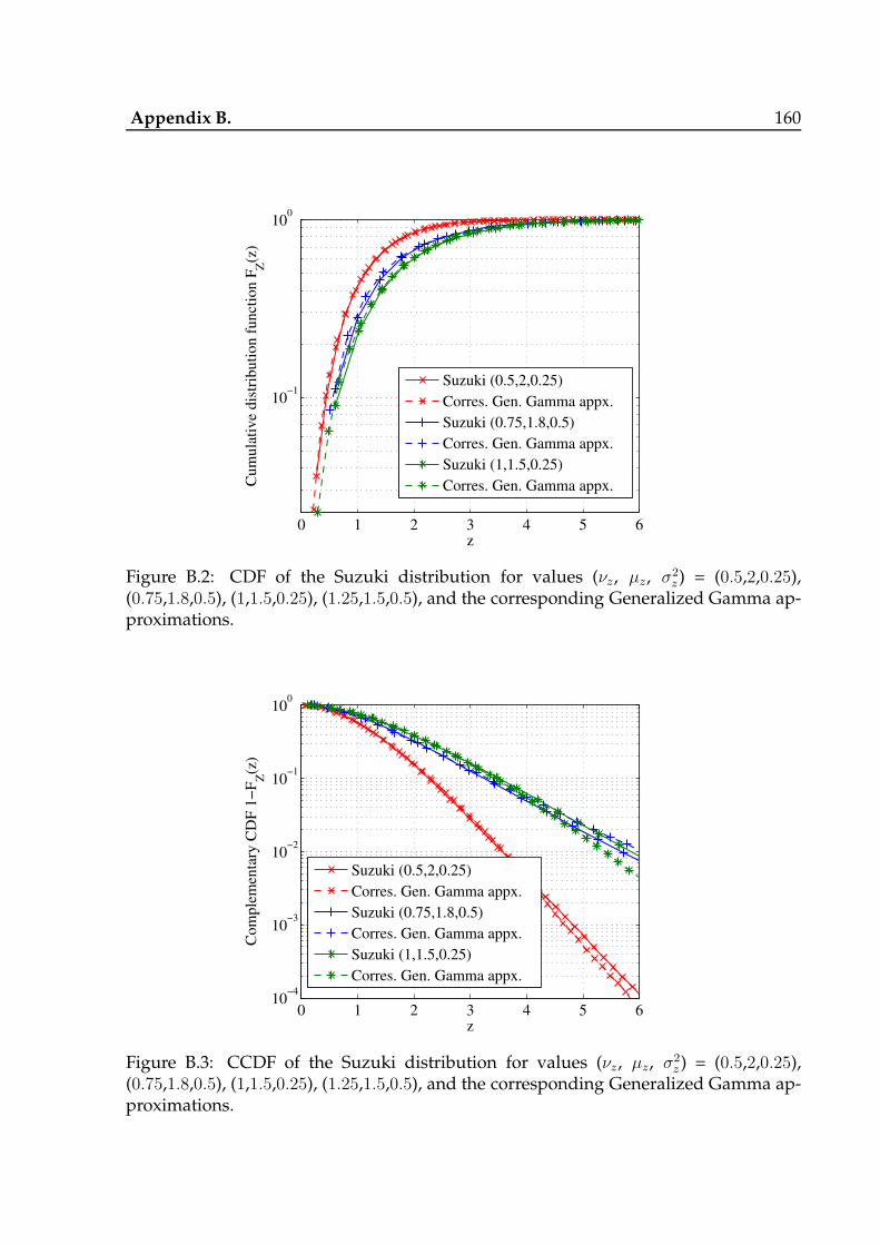
Appendix B. 160

0 1 2 3 4 5 6

10−1

100

z

Cum

ula

tive

dis

trib

uti

on f

unct

ion F

Z(z

)

Suzuki (0.5,2,0.25)

Corres. Gen. Gamma appx.

Suzuki (0.75,1.8,0.5)


Suzuki (1,1.5,0.25)


Figure B.2: CDF of the Suzuki distribution for values (νz, µz, σ2z ) = (0.5,2,0.25),

(0.75,1.8,0.5), (1,1.5,0.25), (1.25,1.5,0.5), and the corresponding Generalized Gamma ap-proximations.

0 1 2 3 4 5 610

−4

10−3

10−2

10−1

100

z

Com

ple

men

tary

CD

F 1

−F

Z(z

)

Suzuki (0.5,2,0.25)


Suzuki (0.75,1.8,0.5)


Suzuki (1,1.5,0.25)


Figure B.3: CCDF of the Suzuki distribution for values (νz, µz, σ2z ) = (0.5,2,0.25),

(0.75,1.8,0.5), (1,1.5,0.25), (1.25,1.5,0.5), and the corresponding Generalized Gamma ap-proximations.

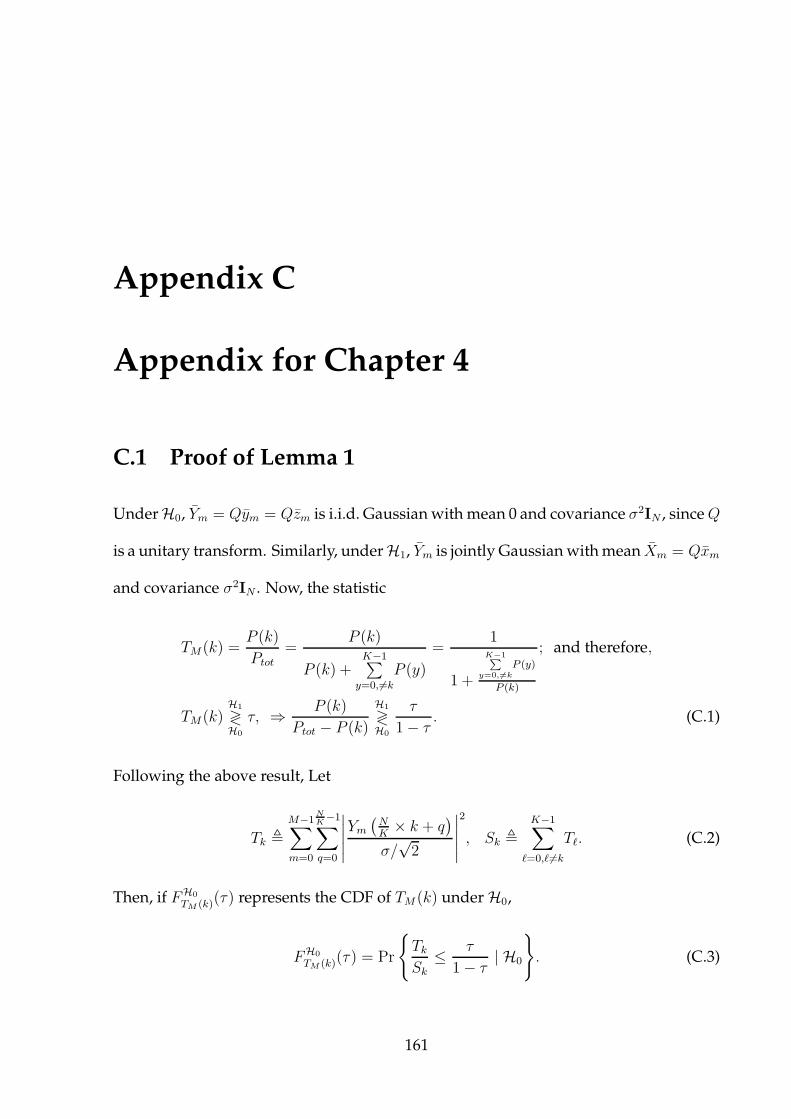
Appendix C


C.1 Proof of Lemma 1

UnderH0, Ym = Qym = Qzm is i.i.d. Gaussianwith mean 0 and covariance σ2IN , sinceQ

is a unitary transform. Similarly, underH1, Ym is jointly Gaussianwithmean Xm = Qxm

and covariance σ2IN . Now, the statistic

TM(k) =P (k)

Ptot=

P (k)

P (k) +K−1∑y=0, 6=k

P (y)

=1

1 +

K−1∑

y=0, 6=kP (y)

P (k)

; and therefore,

TM(k)H1

≷H0

τ, ⇒ P (k)

Ptot − P (k)

H1

≷H0

τ

1− τ. (C.1)

Following the above result, Let

Tk ,M−1∑

m=0

NK−1∑

q=0

∣∣∣∣∣Ym(NK× k + q

)

σ/√2

∣∣∣∣∣

2

, Sk ,K−1∑

ℓ=0,ℓ 6=kTℓ. (C.2)

Then, if FH0

TM (k)(τ) represents the CDF of TM (k) underH0,

FH0

TM (k)(τ) = Pr

TkSk

≤ τ

1− τ| H0

. (C.3)

161

Appendix C. 162

Now, let KX 2Θ(Ψ) represent a chi-squared random variable (RV) with Θ Degrees of

Freedom (DoF), non-centrality parameter Ψ and a scaling factor K. It is easy to see that

under H0, Tk ∼ X 22MNK

(0), k = 1, 2, . . . , K − 1. Also, Sk ∼ X 22M(N−N

K )

(2MK

L−1∑p=0

SNR(p)

).

Next, we use a result due to Patnaik ( [107], [106]), which approximates a X 2Θ(Ψ) RV

with a GX 2Ω(0) RV, where Ω , (Θ+ψ)2

Θ+2ψand G , Θ+ψ

Θ+2ψ. Using this, and the notations in

(4.7), it follows that Sk|H0 ∼ G0X 2D0(0), and Tk|H0 ∼ X 2

2MNK

(0).

Let γ , τ1−τ . Since the statistic TM(k) is a ratio of scaled chi-squared RVs, it follows a

four-parameter beta prime distribution, i.e., [148, chap. 25],

TM(k) =TkSk

∼ β ′(MN

K,D0

2, 1,

1

G0

), with PDF

fH0

TM (k)(ν) =(G0 γ)

MNK (1 +G0γ)

−MNK

−D02

MNK

B(MNK, D0

2

) (C.4)

for γ ∈ [0,∞). The expression for PFA follows from calculating the CDF. A similar

analysis for the statistic underH1 gives the expression of PD.

C.2 Proof of Lemma 2

First, note thatΠ is concave in 0 ≤M ≤ Nh

N. Hence, it suffices to pick theM that satisfies

∂Π∂M

= 0. Define A and B, as in (4.12). Using (4.6), (4.9), and a transformation result for

the Gauss’ hypergeometric function [116, Sec. 9.131], Π can be rewritten as:

Π = K ′[

Γ(AM +BM)

AM Γ(AM)Γ(BM)× (G0γmin)

AM

× (1+G0γmin)1−AM−BM

2F1(1, 1−BM ; 1+AM ;−G0γmin)],

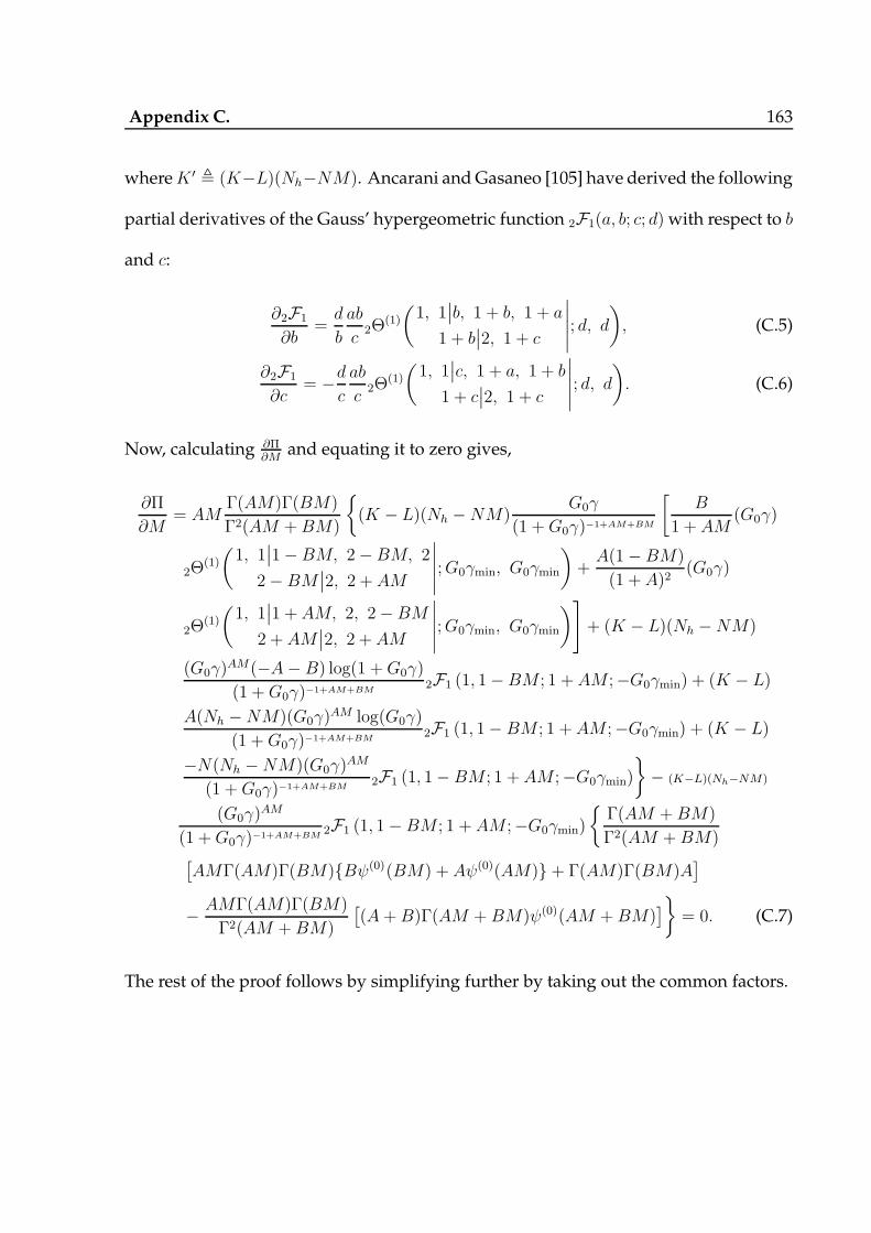
Appendix C. 163

whereK ′ , (K−L)(Nh−NM). Ancarani andGasaneo [105] have derived the following

partial derivatives of the Gauss’ hypergeometric function 2F1(a, b; c; d)with respect to b

and c:

∂2F1

∂b=d

b

ab

c2Θ

(1)

(1, 1

∣∣b, 1 + b, 1 + a

1 + b∣∣2, 1 + c

∣∣∣∣∣; d, d), (C.5)

∂2F1

∂c= −d

c

ab

c2Θ

(1)

(1, 1

∣∣c, 1 + a, 1 + b

1 + c∣∣2, 1 + c

∣∣∣∣∣; d, d). (C.6)

Now, calculating ∂Π∂M

and equating it to zero gives,

∂Π

∂M= AM

Γ(AM)Γ(BM)

Γ2(AM +BM)

(K − L)(Nh −NM)

G0γ

(1 +G0γ)−1+AM+BM

[B

1 + AM(G0γ)

2Θ(1)

(1, 1

∣∣1−BM, 2−BM, 2

2− BM∣∣2, 2 + AM


)+A(1− BM)

(1 + A)2(G0γ)

2Θ(1)

(1, 1

∣∣1 + AM, 2, 2−BM

2 + AM∣∣2, 2 + AM


)]+ (K − L)(Nh −NM)

(G0γ)AM(−A− B) log(1 +G0γ)

(1 +G0γ)−1+AM+BM2F1 (1, 1−BM ; 1 + AM ;−G0γmin) + (K − L)

A(Nh −NM)(G0γ)AM log(G0γ)

(1 +G0γ)−1+AM+BM 2F1 (1, 1− BM ; 1 + AM ;−G0γmin) + (K − L)

−N(Nh −NM)(G0γ)AM

(1 +G0γ)−1+AM+BM 2F1 (1, 1− BM ; 1 + AM ;−G0γmin)

− (K−L)(Nh−NM)

(G0γ)AM

(1 +G0γ)−1+AM+BM 2F1 (1, 1−BM ; 1 + AM ;−G0γmin)

Γ(AM +BM)

Γ2(AM +BM)[AMΓ(AM)Γ(BM)Bψ(0)(BM) + Aψ(0)(AM) + Γ(AM)Γ(BM)A

]

− AMΓ(AM)Γ(BM)

Γ2(AM +BM)

[(A+B)Γ(AM + BM)ψ(0)(AM +BM)

]= 0. (C.7)

The rest of the proof follows by simplifying further by taking out the common factors.

Appendix C. 164

C.3 FAR Algorithm on Lyrtech SFF SDR DP

We now describe our implementation of the FAR algorithm on the Lyrtech SFF SDR DP

(from here on, called DP for short). The block diagram of the DP is as shown in Fig.

C.1, and the hardware circuitry is shown in Fig. C.2. The DP consists of the following

three modules:

1. A Digital Processing Module (DPM), with a Xilinx Virtex-4 SX35 FPGA, TMS320

DM6446 system-on-chip DSP, MSP430 MCU for power management.

2. A Data Conversion Module (DCM), with a 14-bit, 125Msps input channel (ADC),

and dual, 16-bit, 500Msps output channels (DAC). For synchronization, a 10MHz

onboard reference clock is provided, along with two external clock inputs for

ADC and DAC.

3. An RF module (RFM) with a half-duplex (stackable for full-duplex) receiver oper-

ating at RF frequency range of 360-960MHz, selectable bandwidth of 5/20MHz,

IF at 70MHz, with an RF input and output gains of up to 22dB.

Several software development tools are supported by the DP. In particular, we im-

plemented the FAR algorithm on the DPM, using a Model Based Design Kit (MBDK)

released by Lyrtech. Since theMBDKworks in association withMATLABr SimulinkTM ,

the implementation of all the modules are done in MATLAB Simulink.

The parameters chosen for the implementation are as follows. We chose B = 5 MHz

with K = 8 bands, denoted (in the increasing order of their center frequencies) by C4,

C5, C6, C7, C0, C1, C2, C3. The center frequencies of these bands are 395.6, 396.1, 396.65,

397.23, 393.5, 394.15, 394.8, 395.1 MHz, respectively, representing a total bandwidth

Appendix C. 165

of 3.73 Mhz. We set N = 64, M = 128, 256; larger values were not feasible due to

the limitations of the in-built DSP multipliers, in the DPM. We use the NI PXIe1062Q

instrument (Fig. C.3) to generate sinusoids, that model the primary user signals.

The received signal is filtered to a passband of 5 MHz at with center frequency 395.4

MHz, and is down-converted to an Intermediate Frequency (IF) of 30MHz. The IF sig-

nal is sampled at a rate of 125Msps. The sampled IF signal is digitally down-converted

to baseband. The signal is then down-sampled by a factor 25 (since the Nyquist rate

required is 5Msps), each for the in-phase and quadrature components, and is passed

to the FFT block, which outputs the corresponding frequency domain signal in groups

of N samples. These values are sent to the decision statistic block, where the power in

the each band is computed by grouping NKbins for each band and averaging them over

M frames. This calculation corresponds to the FAR statistic, i.e., calculating TM(k),

k = 1, · · · , K, following (4.4). Then, the detection is carried out by comparing the

power in each bin with a user-defined threshold. The decisions made on each band can

be made to be seen on a display (800× 600) provided in the DPM (VPBE and VPFE).

C.3.1 Primary Hop-Instant Identification

It is important for the CR user to know, and synchronize its operation to the hopping in-

stants of the frequency-hopping primary user. A method for estimating the FH bound-

ary for bluetooth signal, with help of a Short Time Fourier Transform (STFT), has been

discussed in [149]. Based on this approach, we propose a technique to identify the FH

boundary by using the already implemented FAR algorithm. This method works under

the assumption that all the primary users are hopping synchronously.

Appendix C. 166

RF Module

DownConversion

30MHz IFto

ADC(125 Msps)

DigitalBasebandConversion(125 Msps)

2-stage D/SAnti-aliasFilter

(5 Msps)

ADCPrecisionControl

FFT(5 Msps)

Dec. StaticComputation

5K

MNMsps

N

M

Dec. MakingBlock

5K

MNMsps

RF CenterFrequency

- BandwidthSelection

ADCChannelGains

Threshold

Display ofChannel Occupancies

VPSS (VPBE)

VPSS (VPFE)

DSP

FPGAModel

Model

Figure C.1: Block Diagram for the Implementation on Lyrtech SFF SDR DP

The time instant at which the CR user powers up and starts sensing the spectrum

will be the reference point in time (from here on, called as the “reference”) for all the

secondary operations. The operational time of the secondary user is also divided into

successive durations ofNh samples starting from the reference, each of which is termed

as Virtual Hopping Period (VHP) of the secondary user. The CR needs to estimate the

difference in time between start of VHP and the start of the hopping period of the

primary, within that particular VHP. Let this time lag be defined as Noffset samples. The

idea is to identify the location in each VHP, where a change in the occupancies of the

primary channels occurs. To this end, in each VHP, the spectrum has to be sensed

repeatedly to know the occupancies. Let Nacc be the difference between the start of

successive sensing operations by the CR (ideally, Nacc should be equal to 1, but due

to hardware and processing limitations, one may have to use a larger Nacc). Since the

Appendix C. 167

Figure C.2: Lyrtech SFF SDR DP circuit board.

sensing duration of the FAR algorithm is Ns, the samples in the successive sensing

operations will be overlapped when Ns > Nacc.

The procedure to estimate Noffset is as follows. Let an occupancy vector U of length

K represent the presence or absence of the primary user on each channel, as declared

by the CR, with an initial value set to the all zero vector [0, · · · , 0] for all the K bands.

Suppose, Nest VHPs are used for estimating the hopping boundary. Starting from the

reference, the spectrum is sensed repeatedly after each Nacc samples. The threshold for

the FAR algorithm is set to satisfy a given, low value of PFA. A vector H of length

Nh

Naccis defined with all elements as zeros. Let id, 0 ≤ id ≤ Nh

Nacc− 1 denote the index of

the sensing operations performed in one VHP. The occupancy vector (U ) for (id + 1)th

sensing operation is logically XOR-ed with that of the (id)th operation. If any one or

more entries of the resultant vector is one, then H(id + 1) is incremented by one. This

process is repeated for all values of id for Nest VHPs. Later, each value of H is compared

Appendix C. 168

Figure C.3: NI PXIe1062Q, used for generating primary signals.

with a threshold hthr and the estimated offset is given by

Noffset = Nacc × id : H(id) ≥ hthr (C.8)

The value of hthr is chosen through simulations.

As an example, consider a case where Noffset = 1040. It is assumed that Nh = 212,

Nest = 100, and the SNR = 6 dB, for each active user. Since Nacc = NM , and the choice

of N is constrained by the hardware, N = 16 is chosen as the FFT size. Therefore,

the choosing Nacc depends on the choice of M . Note that asM increases, the detection

accuracy increases, but the resolution of the boundary detection decreases. For this

example, we will consider M = 1, andM = 32. A threshold value of 0.3 is chosen for

FAR algorithm. The histogram H is computed, and the value of the threshold hthr is set

to be 85 (chosen through simulations). With these values, for the case of M = 1, it is

Appendix C. 169

seen that the above mentioned boundary identification procedure gave the boundary

change index as 65, which results in 65 × 16 ×M = 1040 = Noffset. Similar exercise with

M = 32 gave the boundary change index as 2, which implies 2×16×M = 1040 = Noffset.

Thus, a secondary user can identify the hopping boundary of the FH primary signal

where all the primary users are hopping synchronously. This method can be applied

with slight modifications to the case where the primary users when they are not hop-

ping synchronously, by suitably choosing the threshold for the histogram. More details

can be found in [149].

Appendix D


D.1 Proof of Lemma 3

It is known that the LC rate for Yi, i ∼ M at any given level ℓ is given by [150]

ED1,M

M − 1= 2[P(Yi > ℓ)−P(Yi > ℓ, Yi+1 > ℓ)] (D.1)

from (5.25), it is clear that

P(Yi > ℓ)− P(Yi > ℓ, Yi+1 > ℓ) = P(Xi = 1)−P(Xi = 1, Xi+1 = 1) (D.2)

= Q(ℓ) + P(Xi = 1, Xi+1 = 1) (D.3)

From (5.25), it can be readily shown that

EXiXi+1 = P(Xi = 1, Xi+1 = 1), and (D.4)

EXiEXi+1 = Q2(ℓ) (D.5)

var(Xi) = Q(ℓ)(1−Q(ℓ)) (D.6)

170

Appendix D. 171

Substituting the above into (5.26),

P(Xi = 1, Xi+1 = 1) = Q2(ℓ) +Q(ℓ) (1−Q(ℓ)) ρX (D.7)

Equating (D.1) and (D.7), using (D.3) yields the result.

D.2 Proof of Corollary 4

When ℓ = 0, Q(ℓ) = Q(0) = 12. This implies

ED1,M =M − 1

2(1− ρX), (D.8)

Following a classical result by Rice [151], Kedem has shown that [118]

ED1,M

M − 1=

1

πcos−1 ρX . (D.9)

Substituting for ρX in (D.8), gives the required result.

D.3 Analysis on the non-applicability of ADD and ED

We will use contradiction. Consider any ǫ > 0. Let pf,G, pf,I|G and pf,N|G denote the pf

values when the observations come from the distributions fG , fI and fN respectively,

while the threshold is calculated and fixed based on fG . We need to show that pf,N|G >

pf,G, for any ǫ > 0. Suppose pf,I|G > pf,G, for any ǫ > 0. Then, it is easy to see that

pf,N|G = (1− ǫ)pf,G + ǫpf,I|G

≥ (1− ǫ)pf,G + ǫpf,G = pf,G , (D.10)

Appendix D. 172

with equality only if ǫ = 0. Therefore, for both ED and ADD, it is enough to show that

pf,I|G > pf,G.

First consider ED. It was seen earlier that τED is given by (5.6). Therefore,

pf,G =1−γ(M−12,2σ2GM

)

Γ(M−12

) , pf,I|G =1−γ(M−12,2(σ2G+σ

2I )

M

)

Γ(M−12

) ,

where γ(·, ·) and Γ(·) are the lower incomplete gamma and gamma functions, respec-

tively. By using the well known properties of these functions, it can be easily shown

that [116]

pf,G = exp

−2σ2

G

M

M−12

−1∑

a=0

(2σ2G)a

Maa!

pf,I|G = exp

−2(σ2

G + σ2I )

M

M−12

−1∑

a=0

(2(σ2G + σ2

I ))a

Maa!.

By direct comparison, for same τED, pf,I|G ≥ pf,G , with equality only if σ2I = 0.

Next, consider the ADD. LetA2M represent the Anderson-Darling statistic and letA2

M,G

andA2M,I|G represent the A

2M values when the observations come from fG and fI respec-

tively, while the Zi are calculated using FG. Using (5.9), it suffices to show that the tail

probabilities PA2M,I|G > τADD

> P

A2M,G > τADD

, for large values of τADD where

pf,I|G and pf,G are calculated.

The tail probabilities of A2M,G and A2

M,I|G, for large τADD, can be calculated by using

Hoeffding’s classical result [152]:

PA2M,G > τADD

=∏

v≥2

(1− λ1,0

λv,0

)−1/2

PA2M,I|G > τADD

=∏

v≥2

(1− λ1,1

λv,1

)−1/2

, (D.11)

Appendix D. 173

where 1/λ1,0 = maxv≥1(1/λv,0) and 1/λ1,1 = maxv≥1(1/λv,1).

From (D.11), it can be immediately seen that

PA2M,I|G>τADD

≥PA2M,G >τADD

, if

1

λv,0≥ 1

λv,1, ∀v≥1

We will show that λv,0 ≤ λv,1∀v ≥ 1, by using the technique described by Stephens

[153] to derive theA2M for the case of unknown parameters, the eigenvalues λv,0 and λv,1

can be obtained as a solution to the corresponding Fredholm determinants of K0(·, ·)

and K1(·, ·). The eigenfunctions are chosen to be Ferrer associated Legendre functions,

using which we can write [114]

λv,0 = 2v(2v − 1), ∀v ≥ 1. (D.12)

However, the values of λv,1 have to be obtained numerically, and the first few values

of λv,1 are listed by Stephens [153, Table 2, Column 8]. A direct comparison shows that

λv,0 and λv,1 for any desired level of accuracy (for any finite, large v) show that λv,0 ≤

λv,1.

D.4 On the Wider-Applicability of the Blind Detector

As detailed in Sec. 5.3.3, the statistic used in BD is constructed using the sequence

Bl, l ∈ 1, · · · , n, which is given by

Bl =

∑m−1u=0

Yml−u

m√∑m−1u=0

(Yml−u−Xl)2

m−1/m

, l = 1, · · · , n. (D.13)

Following a classic result in statistics [51], when Yi ∼ N (µ, σ2), i ∈ M,

Appendix D. 174

(i) The random variables, viz., the sample mean and the sample variance are uncor-

related. In fact, they are independent.

(ii) The ratio of sample mean to sample variance, for a small number of samplesm, is

student-t distributed with parameterm− 1.

Shen et al. [53] used the above results to propose the BD, by constructing an Anderson-

Darling detector on the sequence Bl, assuming Gaussian noise, i.e., samples Yi to

be Gaussian distributed. In this section, we discuss the cases when BD can be applied

even when Yi are not Gaussian.

Kendall and Stuart [51, Chap. 30, Sec. 3] have shown that for Yi with an arbitrary

PDF, the asymptotic correlation (as n→∞) between the sample mean and sample vari-

ance (denoted by ρm,v) is given by

ρm,v =κ3√

κ2(κ4 + 2κ22), (D.14)

where κp is the pth-order cumulant of the PDF of Yi. Therefore, as long as the parent

distribution is symmetric and n is large enough, κ3 = 0, and hence ρm,v → 0. Therefore,

provided that the PDF of Yi is symmetric, the samples Bl would still follow the

student-t distribution for large enough n. Additionally, several studies have shown

that this convergence is rapid [51], and is even valid for heavy tailed distributions such

as the SαS distribution.

The t test (i.e., the test on Bl) was originally introduced by Student as a GoFT test

against mean change in the parent distribution [154]. By the property of the SαS dis-

tribution, the pth-ordered moment exists only when α ≥ p. When α < 1, no moment

exists and hence a test on the mean fails. Therefore, when α < 1, Bl no longer follows

Appendix D. 175

a student-t distribution, and BD fails to satisfy the false alarm constraint.

All the above presented arguments are in agreement with our simulation results,

where it was seen that BD performs well even in the presence of non-Gaussian com-

ponents such as class A and B, except for the case when α < 1.

Appendix E

Popular Goodness-of-Fit Tests for the

Gaussian Distribution

In this section, we give mathematical details of some of the popular GoFTs for testing

against samples which are Gaussian distributed with mean 0 and variance σ2. Starting

from the celebrated Pearson’s χ2 test [155], the history of research on designing GoFTs

for testing against various distributions spans over a century, and remains an active

area even today [156]. We choose some of the well-known GoFTs from the literature

and classify them based on an empirical distribution function calculation, correlation

between the samples, higher moments such as skewness and kurtosis, and L-moments.

Unless mentioned otherwise, the main idea in all the tests is to calculate a statistic based

on the observations and derive its distribution underH0 when the number of observa-

tions grows large. This distribution is used to determine the detection threshold that

satisfies a given probability of false-alarm constraint.

In the context of the CR, the tests described below are useful in the scenario when no

knowledge on the primary-only signal, and channel statistics are assumed, in addition

to either of the following scenarios:

176

Appendix E. 177

(i) When only the background noise is present ([53], [52]).

(ii) When the class A [55] component is present along with the background noise,

where the PDF of the combined process can be well approximated by another

Gaussian process ([109], [111]).

Let the observations be denoted by Yi ∈ R, i ∈ M , 1, · · · ,M. Also, let Y(i), i ∈ M

represent the ordered samples from Yi such that Y(1) < · · · < Y(M). Let the observation

vector and the vector of the ordered observations be represented as Y = [Y1, · · · , YM ],

and Y = [Y(1), · · · , Y(M)]. Given Yi, i ∈ M, every GoFT listed in this Appendix answers

whether the hypothesis

H0 : Yi ∼ N (0, σ2) (E.1)

is true or not, and the detection threshold is chosen such that a constraint on the prob-

ability of false-alarm, defined as

Pdeclare “not H0”|H0 true = αf , (E.2)

is satisfied, for a given αf ∈ (0, 1).

E.1 Regression and Correlation Based Tests

The basic idea in regression based tests is as follows. Consider the regression between

the ordered observations and the expected ordered statistics of the standardized ver-

sion of the underlying hypothesized distribution. On a probability plot, this regression

Appendix E. 178

tends to be linear if the hypothesis is true. The tests considered in this section are de-

signed to evaluate the accuracy of the linear fit. The term “correlation” refers to the

strength of the relationship between the sample statistics and their expected value.

E.1.1 The W Test (Shapiro-Wilk Test)

The Shapiro-Wilk test [157], or the W test, is one of the popular and widely used GoFT

for testing against Gaussianity. The idea here is to obtain the best linear unbiased esti-

mates of the mean and variance, for the linear regression. The test is devised as follows.

For the ordered observations Y(i), i ∈ M, let

mi , EY(i), vij , E(Y(i)Y(j)), m , [m1, · · · , mM ], V , (vij)

Y ,1

M

M∑

i=1

Yi, σ ,mTV−1Y

mTV−1m, S2 ,

M∑

i=1

(Y(i) − Y )2, b ,mTV−1mσ

(mTV−1V−1mT )1/2(E.3)

where (·)T represents the transpose of a matrix. The variable b represents the best linear

unbiased estimate of the slope of the linear regression of the ordered observations Y(i)

on the expected valuesmi. The statisticW is defined as

W ,b2

S2=

(M∑i=1

aiY(i)

)2

M∑i=1

(Y(i) − Y

)2 , with aT =mTV−1

(mTV−1V−1mT )1/2. (E.4)

It is important to note that [157]

(1) W is scale and origin invariant.

(2) The distribution ofW depends only onM .

(3) W is statistically independent of S2 and Y , when Yi are Gaussian.

Appendix E. 179

(4) When M = 2K, b =∑M

i=1 aM−i+1(YM−i+1 − Yi), and when M = 2K + 1, b =

∑Mi=1 aM−i+1(YM−i+1−Yi), with aK+1 = 0. Observe the b is same for both even and

oddM .

(5) If ai represents the ith element of vector a, then -ai = aM−i+1.

The distribution of the W statistic has to be obtained through tables [157]. Some other

approximations to theW statistic are also discussed in [157]. TheW statistic is found to

be one of the best tests in literature for testing against Gaussianity. The disadvantages

of this test are the need for a lookup table, and the fact that the tables are available only

upto several tens of number of observations (M ∼ 50).

E.1.2 The Y Test (D’Agostino Test)

The Y test ( [158], [159]) focuses on the correlation between Y(i), i ∈ M and their ex-

pected value. Let

Y ,

∑Mi=1

[i− 1

2(M + 1)

]Y(i)

M2

√1M

∑Mi=1

(Y(i) − Y

) , (E.5)

where Y is the sample mean of Yi, i ∈ M. Now, if Yi, i ∈ M are from a Gaussian

distribution, then [158]

EY =(M − 1)Γ

(M−12

)

2√2πMΓ

(M2

) ≈ 1

2√π= 0.28209479 (E.6)

asd(Y ) ,√EY 2 − E2Y =

(12√3− 37 + 2π

24πM

) 12

≈ 0.02998598√M

(E.7)

where asd(Y ) is the asymptotic standard deviation of the statistic Y .

Appendix E. 180

Therefore, for large enoughM ,

T (Y ) ,Y − EY

asd(Y )∼ N (0, 1). (E.8)

Hence, the Y-test on the observations Yi has the critical region:

Y(i) : T (Y ) > τY

, (E.9)

where the threshold τY is chosen to meet the criterion pf = αf . It is straightforward that

for a given αf , τY is such that

τY = Q−1(αf), (E.10)

where Q−1(·) is the inverse of the Gaussian Q-function.

E.1.3 The Z Test

The Z test [160] follows from the W test, and also exploits the slope of the line between

the sample order statistics and their expected value under Gaussianity. As an approxi-

mation on the statisticW , the statistic Z is defined as

Z ,

(M∑i=1

ciY(i)

)2

M∑i=1

(Y(i) − Y

)2 , (E.11)

where ci , (mTm)1/2mi, with mi = φ[i− 3

8

M+ 14

], and φ(·) is the CDF of a standard normal

distribution. A three parameter lognormal distribution was found to fit the statistic

Z, for various values ofM , details of which are lengthy, and is provided in [160]. The

advantages of this test as compared toW test includes less computational requirements,

and applicability to larger values ofM (up to several thousands).

Appendix E. 181

E.1.4 The QH* Test

Consider the statistic [161]

QH ,1

(M − 1)S1

M−1∑

j=1

Y(i+1) − Y(i)Hi+1 −Hi

, (E.12)

where

Hi , φ−1

[ (i− 3

8

)(M + 1

4

)], S1 ,

[1

M − 1

M∑

i=1

(Y(i) − Y

)2] 1

2

, (E.13)

and φ−1(·) is the inverse of CDF of the standard normal distribution. It is seen that

whenH0 is true, the distribution of QH will have a mean close to unity. Now, consider

another statistic

QH* ,√M(1−QH), (E.14)

which can be used as the test statistic. The distribution of QH* and the detection thresh-

olds are chosen using a lookup table [161, Tab. 2]. The main advantage of this test is

simplicity in the construction of the test statistic, and the disadvantages include appli-

cability to moderately large values ofM , and the need of a lookup table.

E.1.5 The Q Test

The Q test [162] uses similar ideas that are used in the QH* test, and is applicable for

moderate and large values ofM . Let

q1 =

M∑

i=1

aiY(i), q2 =

M∑

i=1

biY(i), (E.15)

Appendix E. 182

where

ai =1

(M − 1)(ui − u1), i = 2, · · · ,M, a1 = −

M∑

i=2

ai (E.16)

b1 = −bM =1

(M − 4)(u1 − u5), b2 = −bM−1 =

1

(M − 4)(u2 − u6)(E.17)

b3 = −bM−2 =1

(M − 4)(u3 − u7), b4 = −bM−3 =

1

(M − 4)(u4 − u8)(E.18)

bi = −bM−i+1 =1

M − 4

(1

ui − ui+4− 1

ui−1 − ui

), i = 5, · · · ,M − 4, (E.19)

and ui , φ−1

[ (i− 3

8

)(M + 1

4

)]

(E.20)

The statistic for the Q-test is given by

Q , log

(q1q2

)(E.21)

It is also known that

EQ = −0.00176− 1.06

M+

6.03

M2(E.22)

σ2Q = 0.011 +

2.9

M− 73.8

M2+

1150.1

M3− 6022.5

M4(E.23)

The Q-test on the observed samples have a critical region:

Y(i) : T (Q) ,

Q− EQ

σQ> τQ

, (E.24)

where τQ is chosen such that pf = αf . The statistic T (Q) follows N (0, 1) closely. The

test is suitable for sample sizes between 10-2000 [162].

Appendix E. 183

E.2 Empirical Distribution Function (EDF) Based Tests

The EDF based tests, as the name suggests, are based on comparison of the Cumulative

Distribution Function (CDF) under the true hypothesis with the EDF estimated from

the samples. These tests are applicable mainly for testing for i.i.d. random variables

with a continuous, known distribution. In this case, it is a Gaussian distribution. When

the parameters of the distribution are unknown and have to be estimated from the

samples, these tests can be used with minor modifications as explained in detail by

Stephens [117].

E.2.1 The D Test (Kolmogorov-Smirnov Test)

Let F(·) represent the CDF of a normal distribution, which is F(x) = φ(x). Given Y(i),

i ∈ M, let Z(i) , F(Y(i)). The statistic for the D test is constructed as follows [117] [163,

and ref. within]:

D+ , max1≤i≤M

[(i

M

)− Z(i)

]

D− , max1≤i≤M

[Z(i) −

(i− 1

M

)]

D , max(D+, D−). (E.25)

The GoFT based on the statistic D against Gaussianity has the following form [117]

(√M + 0.12 +

0.11√M

)D

≁H0

≷∼H0

τD, (E.26)

where the threshold τD is chosen such that pf = αf . The values of τD for some values

of αf is due to Stephens [117].

Appendix E. 184

E.2.2 The W2 Test (Cramer-Von Mises Test)

Let FM(·) represent the EDF estimated fromM samples, which is defined as

FM(t) =1

M

M∑

i=1

IYi≤t, (E.27)

where t ∈ R, and I· is the indicator function. Then the Cramer-Von Mises statistic is

defined as [117]

W 2 ,M

∫ ∞

−∞[FM(x)− F(x)]2 ψ(F(x))dF , (E.28)

where ψ(·) ≥ 0, is a non-negative weight function. With the transformation u = F(x),

the statistic reduces to

W 2 =M

∫ 1

0

[GM(u)− u]2 ψ(u)du, (E.29)

where GM(·) represents the EDF calculated from u1, · · · , uM. It is observed that in

terms of the given observations Z(i) = F(Y(i)) the statistic reduces to

W 2 =

M∑

i=1

[Z(i) −

2i− 1

2M

]2+

(1

12M

), (E.30)

and the test is devised as below [117].

(W 2 +

0.4

M+

0.6

M2

)×(1 +

1

M

)≁H0

≷∼H0

τW . (E.31)

Even in this case, the threshold are to be chosen from the available lookup tables [117],

such that pf = αf .

Appendix E. 185

E.2.3 The A2 Test (Anderson-Darling Test)

The A2 test, or the Anderson-Darling statistic based test [114] is a powerful test for

testing against an alternative hypothesisH1, which is another Gaussian with a positive

mean. The statistic A2 used for this test is a special case of the W2, with the function

ψ(t) = 1F(t)(1−F(t))

. See Chap. 5, Sec. 5.3 for details on this test.

E.3 Omnibus Tests

Omnibus tests are used for testing against Gaussianity based on the moments such as

skewness, or kurtosis, calcuated from the observations. The tests mentioned below are

noted to perform better compared to some of the other tests discussed in the previous

sections.

E.3.1 The K2 Test

The K2-test [164] is an extension Pearson’s χ2 test [155], and detects deviations from

Gaussianity by considering the test statistic K2 to be a linear combination of skewness

and kurtosis. Let mK , 1M

∑Mi=1(Y(i) − Y )K , where Y is the sample mean of Yi, i ∈ M.

The test is devised as follows

i) The skewness-based statistic Z(b1)

(a) Calculate b1 , m3

m3/22

.

(b) Calculate y = b1

(M + 1)(M + 3)

6(M − 2)

1/2

,

β(b1) =3(M2 + 27M − 70)(M + 1)(M + 3)

(M − 2)(M + 5)(M + 7)(M + 9),

w2 , −1 + [2(β(b1)− 1)](1/2), δ =1√logw

, and α =[

2(w2−1)

]1/2.

Appendix E. 186

(c) Compute Z(b1) , δ logyα+[1 +

(yα

)1/2]

ii) The kurtosis-based statistic Z(b2)

(a) Calculate b2 , m4

m22.

(b) Calculate Eb2 =3(M − 1)

(M + 1)and var(b2) =

24M(M − 2)(M − 3)

(M + 1)2(M + 3)(M + 5)

(c) Compute b ,b2 − Eb2√var(b2)

.

(d) Compute β1 =6(M2−5M+2)(M+7)(M+9)

√6(M+3)(M+5)M(M−2)(M−3)

.

(e) Calculate A = 6 + 8β1

[2β1

+√

1 + 4β21

].

(f) Z(b2) ,√

9A2

[(1− 2

9A

)−(

1−2/A

1+b√

2A−4

)1/3]

Finally, the K2 statistic is computed as

K2 , Z2(b1) + Z2(b2) (E.32)

It is known that Z(b1) and Z(b2) closely follow the normal distribution and therefore,

the K2 statistic closely follows a χ2 distribution with 2 degrees of freedom. Therefore,

the K2 test is of the form

K2≁H0

≷∼H0

τK , (E.33)

with τK chosen such that 1−γ(τK

2, 1)= αf . Here, γ(·, ·) represents the lower incomplete

Gamma function.

Appendix E. 187

E.3.2 The G2w Test

The G2w statistic is constructed from the statistic Z(b1) defined in Sec. E.3.1, as follows

[165]. Let

Zw =(M + 2)1/2(w − 3)

3.54, (E.34)

where w = 13.29(log σ − log τ), with

σ ,

√√√√ 1

M

M∑

i=1

(Y(i) − Y )2, τ ,1

M

M∑

i=1

|Y(i) − Y |, (E.35)

where Y is the sample mean of Yi, i ∈ M. Then,

G2w , Z2(b1) + Z2

w. (E.36)

UnderH0, G2w closely follows a χ2 distribution with 2 degrees of freedom. The test, and

the corresponding threshold are calculated similar to that explained in Sec. E.3.1.

E.3.3 The G2∗w Test

The G2∗w test is a simple, easy to calculate approximation to the G2

w statistic, and is given

by

G2∗w ,

M

(M − 2)√

6M+1

b1

2

+ Z2w (E.37)

The rest of the analysis remain similar to the G2w-test.

Appendix E. 188

E.3.4 The L-Moment Skewness-Kurtosis (LSK) Based Test

The test discussed in this section [156] uses a combination of L-skewness and L-kurtosis

to construct the test statistic. The L-moments, introduced by Hosking [166], have sev-

eral advantages as compared to the regular moments. Let Y(i):j represent the ith ordered

sample in a sample size of j. The first few L-moments λl, l = 1, · · · , 4, the L-skewness

κ3, and the L-kurtosis κ4 are defined as

λ1 , EYi, λ2 ,1

2E(Y(2):2 − Y(1):2

), λ3 ,

1

3E(Y(3):3 − 2Y(2):3 + Y(1):3

)

λ4 ,1

4E(Y(4):4 − 3Y(3):4 + 3Y(3):4 − Y(1):4

), κ3 ,

λ3λ2, κ4 ,

λ4λ2. (E.38)

Based on the samples Y(i), the estimates for the L-moments are given as

λ1 =1

M

M∑

i=1

Y(i):M , λ2 =1

2

(M

2

)−1∑∑

i>j

(Y(i):M − Y(j):M

),

λ3 =1

3

(M

3

)−1∑∑∑

i>j>k

(Y(i):M − 2Y(j):M + Y(k):M

),

λ4 =1

4

(M

4

)−1∑∑∑∑

i>j>k>m

(Y(i):M − 3Y(j):M + 3Y(k):M − Y(m):M

)(E.39)

For a Gaussian distribution, it is known that κ3 = 0, and κ4 = 0.1226. Let κ3 and κ4 be

the corresponding estimates from λ3, λ4 and λ2, respectively. Now each of the following

statistics [156]

Z3 ,

(0.1886

M+

0.8

M2

)−1/2

κ3,

Z4 ,

(0.0883

M+

0.68

M2+

4.9

M3

)−1/2

(κ4 − 0.1226) , (E.40)

Appendix E. 189

closely follow a standard Gaussian distribution. Therefore, a test statistic

L3,4 , Z23 + Z2

4 (E.41)

follows a central χ2 distribution with two degrees of freedom. This test is simple in

construction and is independent of the variance σ2. In detection theory, such tests are

referred to as the Constant False Alarm Rate (CFAR) tests. The construction of the test

and selection of the optimal threshold is similar to that used in the K2 test.

As an ending note, it is worth mentioning that when the sample size is small (< 50),

the Shapiro-Wilk (or W) test, and the Kolmogorov-Smirnov (or D) test may be the best

choices ([160] [117]). For larger sample sizes, the choice of an appropriate test depends

on the class of distributions under the alternative hypothesis. For e.g., if the alterna-

tive hypothesis is another Gaussian with an unknown, but non-zero mean, then the

Anderson-Darling (or A2) test could be a suitable choice ([52] [53]). Some of the above

mentioned tests can also be used for a few distributions other than the Gaussian, but

the scenarios under which it is applicable needs to be carefully examined. For e.g.,

the EDF based tests can be used for testing against known, non-Gaussian distributions

with finite mean and variance, provided that the observations are i.i.d.

Bibliography

[1] J. Mitola and G. Maguire, “Cognitive radio: Making the software radios more

personal,” IEEE Pers. Commun., vol. 6, pp. 13–18, Aug. 1999.

[2] J. Mitola, “Cognitive radio for flexible mobile multimedia communications,” in

IEEE International Workshop on Mobile Multimedia Communications (MoMuC), San

Diego, USA, 1999, pp. 3–10.

[3] ——, “Software radio architecture: a mathematical perspective,” IEEE J. Sel. Areas

Commun., vol. 17, no. 4, pp. 514–538, 1999.

[4] J. Mitola III, “Cognitive radio: An integrated agent architecture for software de-

fined radio,” Ph.D. dissertation, Royal Institute of Technology (KTH), Sweden,

May 2000.

[5] D. Cabric, S. M. Mishra, and R. W. Brodersen, “Implementation issues in spec-

trum sensing for cognitive radio,” Proc. Asilomar Conf. on Signals, Syst., and Com-

put., vol. 1, pp. 772–776, Nov. 2004.

[6] D. Cabric and R. Brodersen, “Physical layer design issues unique to cognitive

radio systems,” in Proc. PIMRC, vol. 2, Berlin, DE, 2005, pp. 759–763.

190

BIBLIOGRAPHY 191

[7] G. Ganesan and Y. Li, “Cooperative spectrum sensing in cognitive radio net-

works,” in Proc. DySPAN, Baltimore, USA, 2005, pp. 137–143.

[8] ——, “Agility improvement through cooperative diversity in cognitive radio,” in

Proc. Globecom, vol. 5, St. Louis, USA, 2005, pp. 1–5.

[9] H. Tang, “Some physical layer issues of wide-band cognitive radio systems,” in

Proc. DySPAN, Baltimore, USA, 2005, pp. 151–159.

[10] A. Ghasemi and E. Sousa, “Collaborative spectrum sensing for opportunistic ac-

cess in fading environments,” in Proc. DySPAN, Baltimore, USA, 2005, pp. 131–

136.

[11] ——, “Asymptotic performance of collaborative spectrum sensing under corre-

lated log-normal shadowing,” IEEE Commun. Lett., vol. 11, no. 1, pp. 34–36, 2007.

[12] E. Larsson and G. Regnoli, “Primary system detection for cognitive radio: Does

small-scale fading help?” IEEE Commun. Lett., vol. 11, no. 10, pp. 799–801, 2007.

[13] J. Unnikrishnan and V. Veeravalli, “Cooperative sensing for primary detection in

cognitive radio,” IEEE J. Sel. Topics Signal Process., vol. 2, no. 1, pp. 18–27, Feb.

2008.

[14] D. Bhargavi and C. Murthy, “Performance comparison of energy, matched-filter

and cyclostationarity-based spectrum sensing,” in Proc. SPAWC, Jun. 2010, pp.

1–5.

[15] Y. R. Venugopalakrishna, C. R. Murthy, and D. N. Dutt, “Multiple transmitter

BIBLIOGRAPHY 192

localization and communication footprint identification using energy measure-

ments,” Physical Communication, vol. 9, no. 0, pp. 184–192, 2013. [Online]. Avail-

able: http://www.sciencedirect.com/science/article/pii/S1874490712000717

[16] R. Thomas, L. DaSilva, and A. MacKenzie, “Cognitive networks,” in Proc. DyS-

PAN, Baltimore, USA, 2005, pp. 352–360.

[17] X. Jing, S.-C. Mau, D. Raychaudhuri, and R. Matyas, “Reactive cognitive radio

algorithms for co-existence between IEEE 802.11b and 802.16a networks,” in Proc.

Globecom, vol. 5, St. Louis, USA, 2005, pp. 1–5.

[18] M. Gandetto and C. Regazzoni, “Spectrum sensing: A distributed approach for

cognitive terminals,” IEEE J. Sel. Areas Commun., vol. 25, no. 3, pp. 546–557, 2007.

[19] Y. Chen, G. Yu, Z. Zhang, H.-H. Chen, and P. Qiu, “On cognitive radio networks

with opportunistic power control strategies in fading channels,” IEEE Trans.Wire-

less Commun., vol. 7, no. 7, pp. 2752–2761, 2008.

[20] N. Devroye, P. Mitran, and V. Tarokh, “Cognitive multiple access networks,” in

Proc. IEEE Int. Symp. Inf. Theory, Adelaide, Australia, 2005, pp. 57–61.

[21] K. Lee and A. Yener, “On the achievable rate of three-node cognitive hybrid wire-

less networks,” in International Conference on Wireless Networks, Communications

and Mobile Computing, vol. 2, Wuhan, China, 2005, pp. 1313–1318.

[22] A. Jovicic and P. Viswanath, “Cognitive radio: An information-theoretic perspec-

tive,” in Proc. IEEE Int. Symp. Inf. Theory, Seattle, USA, 2006, pp. 2413–2417.

BIBLIOGRAPHY 193

[23] N. Devroye, P. Mitran, and V. Tarokh, “Achievable rates in cognitive radio chan-

nels,” IEEE Trans. Inf. Theory, vol. 52, no. 5, pp. 1813–1827, 2006.

[24] K. Nagananda, P. Mohapatra, C. R. Murthy, and S. Kishore, “Multiuser cognitive

radio networks: an information-theoretic perspective,” International Journal of

Advances in Engineering Sciences and Applied Mathematics, vol. 5, no. 1, pp. 43–65,

2013. [Online]. Available: http://dx.doi.org/10.1007/s12572-013-0079-1

[25] A. Sharma and C. Murthy, “Group testing based spectrum hole search for cogni-

tive radios,” IEEE Trans. Veh. Technol., vol. PP, no. 99, pp. 1–12, Feb. 2014.

[26] J. Neel, R. Buehrer, J. Reed, and R. P. Gilles, “Game theoretic analysis of a network

of cognitive radios,” in Proc. Midwest Symp. Circuits Syst., vol. 3, Oklahoma, USA,

2002, pp. 409–412.

[27] J. Neel, J. Reed, and R. Gilles, “Convergence of cognitive radio networks,” in Proc.

WCNC, vol. 4, Georgia, USA, 2004, pp. 2250–2255.

[28] C. Rieser, T. Rondeau, C. Bostian, and T. Gallagher, “Cognitive radio testbed: fur-

ther details and testing of a distributed genetic algorithm based cognitive engine

for programmable radios,” in Proc. MILCOM, vol. 3, Monterey, USA, 2004, pp.

1437–1443.

[29] A. Fehske, J. Gaeddert, and J. Reed, “A new approach to signal classification us-

ing spectral correlation and neural networks,” in Proc. DySPAN, Baltimore, USA,

2005, pp. 144–150.

[30] T. Yucek and H. Arslan, “A survey of spectrum sensing algorithms for cognitive

BIBLIOGRAPHY 194

radio applications,” IEEE Communications Surveys & Tutorials, vol. 11, no. 1, pp.

116–130, First Quarter 2009.

[31] I. F. Akyildiz, B. F. Lo, and R. Balakrishnan, “Cooperative spectrum sensing in

cognitive radio networks: A survey,” Phys. Commun., vol. 4, no. 1, pp. 40–62, Mar.

2011.

[32] I. F. Akyildiz, L. Won Yeol, C. V. Mehmet, and M. Shantidev, “A survey on spec-

trummanagement in cognitive radio networks,” IEEE Commun. Mag., vol. 46, pp.

40–48, Apr. 2008.

[33] D. Ariananda, M. Lakshmanan, andH. Nikookar, “A survey on spectrum sensing

techniques for cognitive radio,” Second International Workshop on Cognitive Radio

and Advanced Spectrum Management (CogART), pp. 74–79, May 2009.

[34] “Spectrum Policy Task Force Report,” Federal Communications Commission, US,

Nov. 2002.

[35] C. Cordeiro, K. Challapali, D. Birru, and S. Shankar, “IEEE 802.22: An introduc-

tion to the first wireless standard based on cognitive radios,” Journal of Communi-

cations, vol. 1, no. 1, pp. 38–47, Apr. 2006.

[36] H. L. Van Trees, Detection, estimation, and modulation theory, 1st ed. Wiley, Sep.

2001.

[37] J. N. Tsitsiklis, “Problems in decentralized decision making and computation,”

Ph.D. dissertation, Department of EECS, MIT, Nov. 1984.

BIBLIOGRAPHY 195

[38] R. Tandra and A. Sahai, “SNR walls for signal detection,” IEEE J. Sel. Topics Signal

Process., vol. 2, no. 1, pp. 4–17, 2008.

[39] A. Tkachenko, D. Cabric, and R. Brodersen, “Cognitive radio experiments using

reconfigurable bee2,” in Proc. Asilomar Conf. on Signals, Syst., and Comput., CA,

USA, 2006, pp. 2041–2045.

[40] N. Han, S. Shon, J.-H. Chung, and J.-M. Kim, “Spectral correlation based signal

detection method for spectrum sensing in IEEE 802.22 WRAN systems,” in In-

ternational Conference Advanced Communication Technology (ICACT), vol. 3, Korea,

2006, pp. 1770–1776.

[41] J. Lunden, S. Kassam, and V. Koivunen, “Nonparametric cyclic correlation based

detection for cognitive radio systems,” in International Conference on Cognitive Ra-

dio Oriented Wireless Networks and Communications (CrownCom), Singapore, 2008,

pp. 1–6.

[42] Z. Quan, W. Zhang, S. Shellhammer, and A. Sayed, “Optimal spectral feature

detection for spectrum sensing at very low SNR,” IEEE Trans. Commun., vol. 59,

no. 1, pp. 201–212, 2011.

[43] F. F. Digham, M. S. Alouini, and M. K. Simon, “On the energy detection of un-

known signals over fading channels,” IEEE Trans. Commun., vol. 55, no. 1, pp.

21–24, Jan. 2007.

[44] H. V. Poor, An introduction to signal detection and estimation, 2nd ed. Springer,

New York, 1994.

BIBLIOGRAPHY 196

[45] J. Tsitsiklis, “Decentralized detection by a large number of sensors,” Mathematics

of Control, Signals, and Systems (MCSS), vol. 1, no. 2, pp. 167–182, 1988.

[46] H. Urkowitz, “Energy detection of unknown deterministic signals,” Proc. IEEE,

vol. 55, no. 4, pp. 523–531, Apr. 1967.

[47] S. J. Shellhammer, N. S. Shankar, R. Tandra, and J. Tomcik, “Performance of

power detector sensors of DTV signals in IEEE 802.22 WRANs,” in Proc. TAPAS.

New York, NY, USA: ACM, 2006.

[48] T. M. Cover and J. M. Thomas, Elements of information theory, 2nd ed. John Wiley

and Sons, Inc., 2005.

[49] R. Blahut, “Hypothesis testing and information theory,” IEEE Trans. Inf. Theory,

vol. 20, no. 4, pp. 405–417, Jul. 1974.

[50] Y.-C. Liang, Y. Zeng, E. Peh, and A. T. Hoang, “Sensing-throughput tradeoff for

cognitive radio networks,” IEEE Trans. Wireless Commun., vol. 7, no. 4, pp. 1326–

1337, Apr. 2008.

[51] M. G. Kendall and A. Stuart, The advanced theory of statistics, 2nd ed. Hafner

publishing company, 1961, vol. II.

[52] H. Wang, E.-H. Yang, Z. Zhao, and W. Zhang, “Spectrum sensing in cognitive

radio using goodness of fit testing,” IEEE Trans. Wireless Commun., vol. 8, no. 11,

pp. 5427–5430, Nov. 2009.

[53] L. Shen, H. Wang, W. Zhang, and Z. Zhao, “Blind spectrum sensing for cognitive

BIBLIOGRAPHY 197

radio channels with noise uncertainty,” IEEE Trans. Wireless Commun., vol. 10,

no. 6, pp. 1721–1724, Jun. 2011.

[54] S. Rostami, K. Arshad, and K. Moessner, “Order-statistic based spectrum sensing

for cognitive radio,” IEEE Commun. Lett., vol. 16, no. 5, pp. 592–595, May 2012.

[55] D. Middleton, “Non-gaussian noise models in signal processing for telecommu-

nications: new methods an results for class A and class B noise models,” IEEE

Trans. Inf. Theory, vol. 45, no. 4, pp. 1129–1149, May 1999.

[56] S. Gurugopinath, C. R. Murthy, and V. Sharma, “Error exponent analysis of

energy-based Bayesian spectrum sensing under fading channels,” in Proc. Globe-

com, Houston, USA, Dec. 2011, pp. 1–5.

[57] G. Sanjeev, K. V. K. Chaythanya, and C. R. Murthy, “Bayesian decentralized spec-

trum sensing in cognitive radio networks,” in Int. Conf. on Sig. Proc. and Commun.

(SPCOM), Bangalore, India, Jul. 2010, pp. 1–5.

[58] S. Gurugopinath, “Near-optimal detection thresholds for bayesian spectrum

sensing under fading,” in Proc. SPCOM, Bangalore, India, Jul. 2014, pp. 1–6.

[59] S. Gurugopinath, R. Akula, C. R. Murthy, R. Prasanna, and B. Amruthur, “Spec-

trum sensing with a frequency-hopping primary: from theory to practice,” in

Proc. ICC, Sydney, Australia, Jun. 2014, pp. 1–6.

[60] S. Gurugopinath, C. R. Murthy, and C. S. Seelamantula, “Zero-crossings based

spectrum sensing under noise uncertainties,” in Proc. NCC, Kanpur, India, Mar.

2014, pp. 1–6.

BIBLIOGRAPHY 198

[61] S. Gurugopinath, “Multi-dimensional goodness-of-fit tests for spectrum sensing

based on stochastic distances,” in Proc. SPCOM, Bangalore, India, Jul. 2014, pp.

1–6.

[62] S. Haykin, “Cognitive radio: Brain empowered wireless communications,” IEEE

J. Sel. Areas Commun., vol. 23, pp. 201–220, Feb. 2005.

[63] E. Visotsky, S. Kuffner, and R. Peterson, “On collaborative detection of TV trans-

missions in support of dynamic spectrum sharing,” in Proc. DySPAN, Baltimore,

USA, 2005, pp. 338–345.

[64] S. Mishra, A. Sahai, and R. Brodersen, “Cooperative sensing among cognitive

radios,” in Proc. ICC, vol. 4, Istanbul, Turkey, 2006, pp. 1658–1663.

[65] Y.-C. Liang, K.-C. Chen, G. Li, and P. Mahonen, “Cognitive radio networking

and communications: an overview,” IEEE Trans. Veh. Technol., vol. 60, no. 7, pp.

3386–3407, Sep. 2011.

[66] M. Lopez-Benıtez and F. Casadevall, “Versatile, accurate, and analytically

tractable approximation for the Gaussian Q-function,” IEEE Trans. Commun.,

vol. 59, no. 4, pp. 917–922, Apr. 2011.

[67] A.Makarfi andK. Hamdi, “Interference analysis of energy detection for spectrum

sensing,” IEEE Trans. Veh. Technol., vol. 62, no. 6, pp. 2570–2578, Jul. 2013.

[68] P. Sofotasios, E. Rebeiz, L. Zhang, T. Tsiftsis, D. Cabric, and S. Freear, “Energy

detection based spectrum sensing over κ−µ and κ−µ extreme fading channels,”

IEEE Trans. Veh. Technol., vol. 62, no. 3, pp. 1031–1040, Mar. 2013.

BIBLIOGRAPHY 199

[69] J. F. Chamberland and V. Veeravalli, “Decentralized detection in sensor net-

works,” IEEE Trans. Signal Process., vol. 51, no. 2, pp. 407–416, Feb. 2003.

[70] Y. Lee and Y. Sung, “Generalized Chernoff information for mismatched Bayesian

detection and its application to energy detection,” IEEE Signal Process. Lett.,

vol. 19, no. 11, pp. 753–756, Nov. 2012.

[71] P. K. Varshney, Distributed detection and data fusion, 1st ed. Springer-Verlag New

York, Inc., 1996.

[72] Y. Zeng, Y. C. Liang, and R. Zhang, “Blindly combined energy detection for spec-

trum sensing in cognitive radio,” IEEE Signal Process. Lett., vol. 15, pp. 649–652,

2008.

[73] P. Wang, J. Fang, N. Han, and H. Li, “Multiantenna-assisted spectrum sensing for

cognitive radio,” IEEE Trans. Veh. Technol., vol. 59, no. 4, pp. 1791–1800, May 2010.

[74] A. Pandharipande and J. Linnartz, “Performance analysis of primary user detec-

tion in a multiple antenna cognitive radio,” in Proc. ICC, Glasgow, UK, Jun. 2007,

pp. 6482–6486.

[75] S. Atapattu, C. Tellambura, and H. Jiang, “Energy detection based cooperative

spectrum sensing in cognitive radio networks,” IEEE Trans. on Wireless Commun.,

vol. 10, no. 4, pp. 1232 –1241, Apr. 2011.

[76] W. Zhang, R. Mallik, and K. Letaief, “Optimization of cooperative spectrum sens-

ing with energy detection in cognitive radio networks,” IEEE Trans. Wireless Com-

mun., vol. 8, no. 12, pp. 5761–5766, Dec. 2009.

BIBLIOGRAPHY 200

[77] H. Hashemi, “The indoor radio propagation channel,” Proc. IEEE, vol. 81, no. 7,

pp. 943–968, Jul. 1993.

[78] A. Iyer, K. K. Chintalapudi, V. Navda, R. Ramjee, V. Padmanabhan, and C. R.

Murthy, “Spectrum sensing sans frontieres,” in 8th USENIX Symposium on Net-

worked Systems Design and Implementation (NSDI ’11), Boston, USA, Mar. 2011.

[79] S. Zheng, P.-Y. Kam, Y.-C. Liang, and Y. Zeng, “Spectrum sensing for digital pri-

mary signals in cognitive radio: A Bayesian approach for maximizing spectrum

utilization,” IEEE Trans.Wireless Commun., vol. 12, no. 4, pp. 1774–1782, Apr. 2013.

[80] D. Cabric, A. Tkachenko, and R. Brodersen, “Spectrum sensing measurements of

pilot, energy, and collaborative detection,” in Proc. MILCOM, Washington D.C.,

USA, Oct. 2006, pp. 1–7.

[81] A. Sonnenschein and P. M. Fishman, “Radiometric detection of spread-spectrum

signals in noise of uncertain power,” IEEE Trans. Aerosp. Electron. Syst., vol. 28,

pp. 654–660, Jul. 1992.

[82] P. Barsocchi, “Channel models for terrestrial wireless communications: A sur-

vey,” available at http://puma.isti.cnr.it/dfdownload.php?ident=/cnr.isti/2006-TR-16,

2006.

[83] Z. Li, F. Yu, and M. Huang, “A distributed consensus-based cooperative

spectrum-sensing scheme in cognitive radios,” IEEE Trans. Veh. Technol., vol. 59,

no. 1, pp. 383–393, Jan. 2010.

BIBLIOGRAPHY 201

[84] Z. Chair and P. K. Varshney, “Optimal data fusion in multiple sensor detection

systems,” IEEE Trans. Aerosp. Electron. Syst., vol. 22, no. 1, pp. 98–101, Jan. 1986.

[85] J. Filho and M. Yacoub, “Simple precise approximations to Weibull sums,” IEEE

Commun. Lett., vol. 10, no. 8, pp. 614–616, Aug. 2006.

[86] M. Di Renzo, F. Graziosi, and F. Santucci, “Further results on the approximation

of log-normal power sum via Pearson type IV distribution: A general formula

for log-moments computation,” IEEE Trans. Commun., vol. 57, no. 4, pp. 893–898,

Apr. 2009.

[87] R. Srinivasan, Importance sampling: Applications in communications and detection.

Springer Verlag, 2002.

[88] S. Astaneh and S. Gazor, “Cooperative spectrum sensing over mixture-nakagami

channels,” IEEE Commun. Lett., vol. 2, no. 3, pp. 259–262, 2013.

[89] E. Axell, G. Leus, E. Larsson, and H. Poor, “Spectrum sensing for cognitive radio

: State-of-the-art and recent advances,” IEEE Signal Process. Mag., vol. 29, no. 3,

pp. 101–116, May 2012.

[90] X. Li and X.-B. Li, “Common fallacies in applying hypothesis testing,” in 11th Int.

Conf. on Information Fusion, Cologne, Germany, Jul. 2008, pp. 1–8.

[91] M.-S. Alouini andM. K. Simon, “Performance of generalized selection combining

over Weibull fading channels: Research articles,” Wireless. Commun. and Mobile

Comput., vol. 6, pp. 1077–1084, Dec. 2006.

BIBLIOGRAPHY 202

[92] “Coverage prediction for mobile radio systems operating in the 800/900 MHz

frequency range,” IEEE Trans. on Veh. Tech., vol. 37, no. 1, pp. 3–72, 1988.

[93] S. Y. D. Dubey, “Normal and weibull distributions,” Naval Research Logistics,

no. 14, pp. 69–79, 1967.

[94] F. Hernandez and R. A. Johnson, “The large-sample behavior of transformations

to normality,” Journal of the American Statistical Association, vol. 75, no. 372, pp.

855–861, 1980.

[95] N. Shepherd, “Radio wave loss deviation and shadow loss at 900 MHz,” IEEE

Trans. on Veh. Tech., vol. 26, no. 4, pp. 309–313, 1977.

[96] A. Coulson, A. Williamson, and R. Vaughan, “Improved fading distribution for

mobile radio,” IEE Proc. Commun., vol. 145, no. 3, pp. 197–202, Jun. 1998.

[97] D.-C. Oh and Y.-H. Lee, “Low complexity fft based spectrum sensing in bluetooth

system,” in Proc. VTC, 2009, pp. 1–5.

[98] G. R. Cooper, “Detection of frequency-hop signals,” IEEE MILCOM, vol. 1, pp.

1–5, Oct. 1986.

[99] L. Miller, J. Lee, and D. Torrieri, “Frequency-hopping signal detection using par-

tial band coverage,” IEEE Trans. Aerosp. Electron. Syst., vol. 29, pp. 540–553, Apr.

1993.

[100] R. A. Dillard and G. M. Dillard, “Likelihood-ratio detection of frequency-hopped

signals,” IEEE Trans. Aerosp. Electron. Syst., vol. 32, pp. 543–553, April 1996.

BIBLIOGRAPHY 203

[101] Z. Chen, N. Guo, and R. Qiu, “Demonstration of real-time spectrum sensing for

cognitive radio,” in Proc. MILCOM, Oct 2010, pp. 323–328.

[102] Y. Hur, J. Park, K. Kim, J. Lee, K. Lim, C. H. Lee, S. H. Kim, and J. Laskar, “A

cognitive radio (cr) testbed system employing a wideband multi-resolution spec-

trum sensing (mrss) technique,” Proc. VTC, pp. 1–5, Sep. 2006.

[103] Z. Peng, Q. Robert, and N. Guo, “Demonstration of spectrum sensing with

blindly learned features,” IEEE Commun. Lett., vol. 15, pp. 548–550, May 2011.

[104] D. Kun and N. A. Morgan, “A new low-cost cfar detector for spectrum sensing

with cognitive radio systems,” IEEE Aerospace Conference, pp. 1–8, Mar. 2008.

[105] L. U. Ancarani and G. Gasaneo, “Derivatives of any order of the hypergeometric

function 2F1(a, b; c; z)with respect to the parameters a, b and c,” Journal of Physics

A: Mathematical and Theoretical, vol. 43, no. 8, p. 085210, 2010.

[106] H. Urkowitz, “Energy detection of unknown deterministic signals,” Proc. IEEE,

vol. 55, pp. 523–531, Apr. 1967.

[107] P. B. Patnaik, “The non-central χ2- and F-distribution and their applications,”

Biometrika, vol. 36, no. 1/2, pp. 202–232, Jun. 1949.

[108] G. Chavali, “Signal detection andmodulation classification in non-gaussian noise

environments,” Ph.D. dissertation, Virginia Polytechnic Institute and State Uni-

versity, Jul. 2012.

[109] K. S. Vastola, “Threshold detection in narrow-band non-gaussian noise,” IEEE

Trans. Commun., vol. 32, no. Feb., pp. 134–139, 1984.

BIBLIOGRAPHY 204

[110] J. Miller and J. Thomas, “The detection of signals in impulsive noise modeled as

a mixture process,” IEEE Trans. Commun., vol. 24, no. 5, pp. 559–563, May 1976.

[111] B. Aazhang and H. Poor, “Performance of DS/SSMA communications in impul-

sive channels–part I: Linear correlation receivers,” IEEE Trans. Commun., vol. 35,

no. 11, pp. 1179–1188, Nov. 1987.

[112] K. Jitvanichphaibool, Y.-C. Liang, and Y. Zeng, “Spectrum sensing using multiple

antennas for spatially and temporally correlated noise environments,” in 2010

IEEE Symposium on New Frontiers in Dynamic Spectrum, Singapore, Apr. 2010, pp.

1–7.

[113] V. Pohl, F. Suratman, A. Zoubir, and H. Boche, “Spectrum sensing for cognitive

radio architectures based on sub-nyquist sampling schemes,” in 2011 International

ITG Workshop on Smart Antennas (WSA), Aachen, Germany, Feb. 2011, pp. 1–8.

[114] T. W. Anderson and D. A. Darling, “Asymptotic theory of certain ”Goodness of

Fit” criteria based on stochastic processes,” Ann. Math. Statist., vol. 23, no. 2, pp.

193–212, Jun. 1952.

[115] B. Kedem and E. Slud, “Time series discrimination by higher order crossings,”

The Annals of Statistics, vol. 10, no. 3, pp. 786–794, Sep. 1982.

[116] I. Gradshteyn and I. Ryzhik, Tables of integrals, series and products, 7th ed. Aca-

demic Press, 2007.

[117] M. A. Stephens, “EDF statistics for goodness of fit and some comparisons,” Jour-

nal of the American Statistical Association, vol. 69, no. 347, pp. 730–737, Sep. 1974.

BIBLIOGRAPHY 205

[118] B. Kedem, “Spectral analysis and discrimination by zero-crossings,” Proc. IEEE,

vol. 74, no. 11, pp. 1477–1493, Nov. 1986.

[119] B. L. Welch, “On linear combinations of several variances,” Journal of the American

Statistical Association, vol. 51, no. 273, pp. 132–148, Mar. 1956.

[120] M. West, “On scale mixtures of normal distributions,” Biometrika, vol. 74, no. 3,

pp. 646–648, 1987.

[121] R. S. Blum, Y. Zhang, B. M. Sadler, and R. J. Kozick, “On the approximation of

correlated non-gaussian noise pdfs using gaussian mixture models,” in Confer-

ence on the Applications of Heavy Tailed Distributions in Economics, Engineering and

Statistics, Jun. 1999.

[122] S. Shellhammer, “Spectrum sensing in IEEE 802.22,” in First Workshop on Cognitive

Info. Process.(CIP 2008), Santorini, Greece, 2008.

[123] Y. Zeng, Y.-C. Liang, A. T. Hoang, and R. Zhang, “A review on spectrum sensing

for cognitive radio: challenges and solutions,” EURASIP J. Adv. Signal Process.,

vol. 2010, Jan. 2010.

[124] T. Feng, T. Field, and S. Haykin, “Stochastic differential equation theory applied

to wireless channels,” IEEE Trans. Commun., vol. 55, no. 8, pp. 1478–1483, 2007.

[125] S. Krusevac, P. Rapajic, and R. Kennedy, “Channel capacity estimation for MIMO

systems with correlated noise,” in Proc. Globecom, vol. 5, St. Louis, USA, Dec.

2005, pp. 1–5.

BIBLIOGRAPHY 206

[126] V. Aalo and R. Viswanathan, “Asymptotic performance of a distributed detection

system in correlated gaussian noise,” IEEE Trans. Signal Process., vol. 40, no. 1, pp.

211–213, Jan. 1992.

[127] R. Zhang, T. J. Lim, Y.-C. Liang, and Y. Zeng, “Multi-antenna based spectrum

sensing for cognitive radios: A GLRT approach,” IEEE Trans. Commun., vol. 58,

no. 1, pp. 84–88, Jan. 2010.

[128] S. Kritchman and B. Nadler, “Non-parametric detection of the number of signals:

Hypothesis testing and randommatrix theory,” IEEE Trans. Signal Process., vol. 57,

no. 10, pp. 3930–3941, Oct. 2009.

[129] P. Bianchi, M. Debbah, M. Maida, and J. Najim, “Performance of statistical tests

for single-source detection using random matrix theory,” IEEE Trans. Inf. Theory,

vol. 57, no. 4, pp. 2400–2419, Apr. 2011.

[130] S. John, “The distribution of a statistic used for testing sphericity of normal dis-

tributions,” Biometrika, vol. 59, no. 1, pp. 169–173, Apr. 1972.

[131] Y. Zeng and Y. C. Liang, “Eigenvalue-based spectrum sensing algorithms for cog-

nitive radio,” IEEE Trans. Commun., vol. 57, no. 6, pp. 1784–1793, Jun. 2009.

[132] F. Penna, R. Garello, and M. Spirito, “Cooperative spectrum sensing based on the

limiting eigenvalue ratio distribution in wishart matrices,” IEEE Commun. Lett.,

vol. 13, no. 7, pp. 507–509, Jul. 2009.

[133] L. Wei and O. Tirkkonen, “Spectrum sensing in the presence of multiple primary

users,” IEEE Trans. Commun., vol. 60, no. 5, pp. 1268–1277, May 2012.

BIBLIOGRAPHY 207

[134] J. W.Mauchly, “Significance test for sphericity of a normal n-variate distribution,”

The Annals of Mathematical Statistics, vol. 11, no. 2, pp. 204–209, Jun. 1940.

[135] R. Bartoszynski, D. K. Pearl, and J. Lawrence, “A multidimensional goodness-of-

fit test based on interpoint distances,” Journal of the American Statistical Association,

vol. 92, no. 438, pp. 577–586, Jun. 1997.

[136] M. Salicru, D. Morales, M. Menendez, and L. Pardo, “On the applications of di-

vergence type measures in testing statistical hypotheses,” Journal of Multivariate

Analysis, vol. 51, no. 2, pp. 372–391, Nov. 1994.

[137] J.-F. Maa, D. K. Pearl, and R. Bartoszynski, “Reducing multidimensional two-

sample data to one-dimensional interpoint comparisons,” The Annals of Statistics,

vol. 24, no. 3, pp. 1069–1074, Jun. 1996.

[138] A. Nielsen, H. Skriver, and K. Conradsen, “Complex wishart distribution based

analysis of polarimetric synthetic aperture radar data,” in International Workshop

on the Analysis of Multi-temporal Remote Sensing Images (MultiTemp), Provinciehuis

Leuven, Belgium, 2007, pp. 1–6.

[139] A. C. Frery, A. D. C. Nascimento, and R. J. Cintra, “Information theory and image

understanding: An application to polarimetric SAR imagery,” Chilean Journal of

Statistics, vol. 2, no. 2, pp. 81–101, Sep. 2011.

[140] F. Yilmaz and M.-S. Alouini, “Sum of weibull variates and performance of diver-

sity systems.” in Proc. IWCMC, Leipzig, Germany, Jun. 2009, pp. 247–252.

BIBLIOGRAPHY 208

[141] A. Winkelbauer, “Moments and absolute moments of the normal distribution,”

Arxiv preprint arXiv:1209.4340, Sep. 2012.

[142] R. L. Winkler, G. M. Roodman, and R. R. Britney, “The determination of partial

moments,” Management Science, vol. 19, no. 3, pp. pp. 290–296, 1972.

[143] S. Gezici, Z. Sahinoglu, and H. Poor, “On the optimality of equal gain combining

for energy detection of unknown signals,” IEEE Commun. Lett., vol. 10, no. 11, pp.

772–774, Nov. 2006.

[144] I. Hoballah and P. Varshney, “Distributed bayesian signal detection,” IEEE Trans.

Inf. Theory, vol. 35, no. 5, pp. 995–1000, Sep. 1989.

[145] I. Csiszar and J. Korner, Information theory coding theorems for discrete memoryless

systems, 1st ed. Academic Press, Inc. (London) Ltd., 1981.

[146] N. C. Sagias and G. S. Tombras, “On the cascaded Weibull fading channel

model,” Journal of the Franklin Institute, vol. 344, no. 1, pp. 1–11, 2007.

[147] C. Withers and S. Nadarajah, “A generalized Suzuki distribution,” Wireless Pers.

Commun., pp. 1–24, 2010, 10.1007/s11277-010-0095-4.

[148] N. Johnson, S. Kotz, and N. Balakrishnan, Continuous Univariate Distributions,

2nd ed. Wiley & Sons, 1995, vol. 2.

[149] A. Gok, S. Joshi, J. Villasenor, and C. Danijela., “Estimating the number of fre-

quency hopping interferers using spectral sensing with time and frequency offset

measurements,” IEEE MILCOM, pp. 1–7, Oct. 2009.

BIBLIOGRAPHY 209

[150] L. J. Tick and P. Shaman, “Sampling rates and appearance of stationary gaussian

processes,” Technometrics, vol. 8, no. 1, pp. 91–106, Feb. 1966.

[151] S. O. Rice, “Mathematical analysis of random noise,” Bell System Tech. J., vol. 23,

no. 3, pp. 282–332, Jul. 1944.

[152] W. Hoeffding, “On a theorem of V. M. Zolotarev,” Thoer. Probability Appl., vol. 9,

pp. 89–92, 1964.

[153] M. A. Stephens, “Asymptotic results for goodness-of-fit statistics with unknown

parameters,” The Annals of Statistics, vol. 4, no. 2, pp. 357–369, Mar. 1976.

[154] Student, “The probable error of a mean,” Biometrika, vol. 6, no. 1, pp. 1–25, Mar.

1908.

[155] K. Pearson, “On the criterion that a given system of deviations from the probable

in the case of a correlated system of variables is such that it can be reasonably

supposed to have arisen from random sampling,” Philosophical Magazine Series,

vol. 50, p. 157175, 1908.

[156] A. Harri and K. H. Coble, “Normality testing: two new tests using L-moments,”

Journal of Applied Statistics, vol. 38, no. 7, pp. 1369–1379, 2011.

[157] S. S. Shapiro andM. B.Wilk, “An analysis of variance test for normality (complete

samples),” Biometrika, vol. 3, no. 52, Dec. 1965.

[158] R. B. D’Agostino, “An omnibus test of normality for moderate and large size

samples,” Biometrika, vol. 58, no. 2, pp. 341–348, Aug. 1971.

BIBLIOGRAPHY 210

[159] ——, “Small sample probability points for the D test of normality,” Biometrika,

vol. 59, no. 1, pp. 219–221, Apr. 1972.

[160] P. Royston, “Approximating the shapiro-wilkW-test for non-normality,” Statistics

and Computing, vol. 2, no. 3, pp. 117–119, Oct. 1992.

[161] L. Chen and S. S. Shapiro, “An alernative test for normality based on normalized

spacings,” Journal of Statistical Computation and Simulation, vol. 53, no. 12, pp. 269–

287, Dec. 1995.

[162] P. Zhang, “Omnibus test of normality using the q statistic,” Journal of Applied

Statistics, vol. 26, no. 4, pp. 519–528, Oct. 1999.

[163] N. Smirnov, “Table for estimating the goodness of fit of empirical distributions,”

The Annals of Mathematical Statistics, vol. 19, no. 2, pp. 279–281, 1948.

[164] R. B. D’Agostino, A. Belanger, and J. D’Agostino, Ralph B., “A suggestion for

using powerful and informative tests of normality,” The American Statistician,

vol. 44, no. 4, pp. 316–321, Nov. 1990.

[165] E. Seier, “Comparison of tests for univariate normality,” Statistics on the Internet,

pp. 1–17, Jan. 2002.

[166] J. R. M. Hosking, “L-moments: Analysis and estimation of distributions using

linear combinations of order statistics,” Journal of the Royal Statistical Society. Series

B (Methodological), vol. 52, no. 1, pp. 105–124, 1990.

Sanjeev Gurugopinath (IISc 2015)

Chandra Ramabhadra Murthy (UCSD 2006)KVS Hari (UCSD 1990)

David Wipf (UCSD)

Bhaskar D. Rao (USC 1983)

Sun-Yuan Kung (Stanford 1977)

Thomas Kailath (MIT 1961)

Jimmy K. Omura (MIT 1966)

Babak Hassibi (MIT 1996)Ali H. Sayed (MIT 1992)

John McReynolds Wozencraft (MIT 1957)

David Forney Jr. (MIT 1965)

Robert Mario Fano (MIT 1947)

Ernst Adolph Guillemin (1926)

Arnold Johannes Wilhelm Sommerfeld (1891)

C. L. Ferdinand (Carl Louis) Lindemann (1873)

David Hilbert (1885)

Martin Kutta (1900)

Hermann Minkowski (1885)

Rudolf Otto Sigismund Lipschitz (1853)

Julius Plucker (1823)Gustav Peter Lejeune Dirichlet (1827)

Martin Ohm (1811)

Leo Pochhammer (1863)

Jean-Bapiste Joseph Fourier Simeon Denis Poisson (1800)

Joseph Louis Lagrange (1754) Pierre Simon Laplace

Jean LeRond d’AlembertLeonhard Euler (1726)

Johann Bernoulli (1694)

Jacob Bernoulli (1676,84)

Nicolas Malebranche (1672)

Gottfried Wilhelm Leibniz (1672)

Christian Huygens (1647,55)Erhard Weigel (1650)

Philipp Mller (1604)

Christoph Meurer (1582)

Moritz Valentin Steinmetz (1550, 67)

Georg Joachim von Leuchen Rheticus (1535)

Nicolaus (Mikoaj Kopernik) Copernicus (1499)

Christian Ludwig Gerling (1812)

Carl Friedrich Gauss (1799)

Friedrich Leibniz (1622)

Jakob Thomasius (1643)

Otto Mencke (1665)

Johann Wichmannshausen (1685)

Christian Hausen (1713)

Abraham Kastner (1739)

Johann Friedrich Pfaff (1786)

Ernst EduardKummer (1831)

JohannElert Bode

spectrum sensing techniques for cognitive radio...

Documents