speculative bubbles, heterogeneous beliefs, and … · speculative bubbles can occur in markets...

Speculative Bubbles,Heterogeneous Beliefs,

and Learning

******

Jan WernerUniversity of Minnesota

..

NBP, Warsaw, June 2018 – p. 1/31

Asset Price Bubbles

Recent Price Bubbles:

Japanese Bubble of 1980s’,

Dot.com Bubble,

US Housing Bubble,

Chinese Warrant Bubble

Bitcoin Bubble,

Dow Jones at 26,000 (?).

Understanding Price Bubbles.

What should policy makers do about price bubbles?


Understanding Asset Price Bubbles

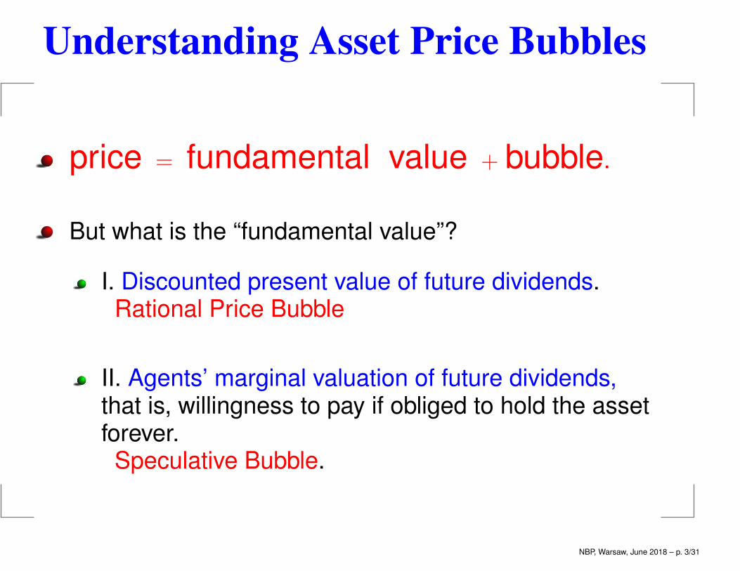
price = fundamental value + bubble.

But what is the “fundamental value”?

I. Discounted present value of future dividends.Rational Price Bubble

II. Agents’ marginal valuation of future dividends,that is, willingness to pay if obliged to hold the assetforever.

Speculative Bubble.


Rational Price Bubble

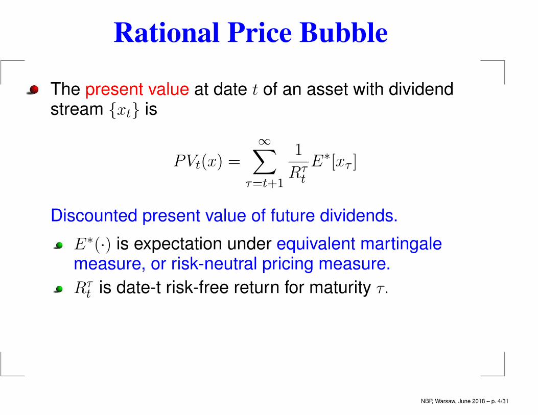
The present value at date t of an asset with dividendstream {xt} is

PVt(x) =

∞∑τ=t+1

1

Rτt

E∗[xτ ]

Discounted present value of future dividends.

E∗(·) is expectation under equivalent martingalemeasure, or risk-neutral pricing measure.

Rτt is date-t risk-free return for maturity τ.


Speculative Bubble

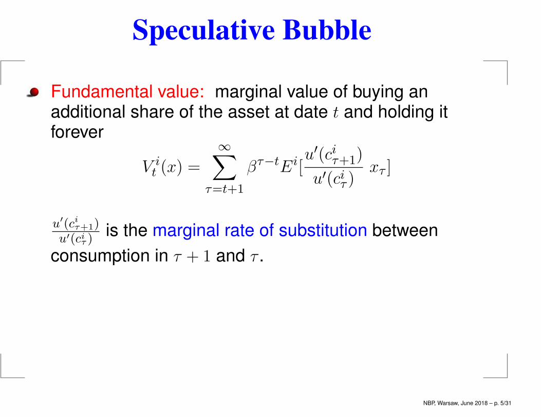
Fundamental value: marginal value of buying anadditional share of the asset at date t and holding itforever

V it (x) =

∞∑τ=t+1

βτ−tEi[u′(ciτ+1)

u′(ciτ )xτ ]

u′(ciτ+1)u′(ciτ )

is the marginal rate of substitution between

consumption in τ + 1 and τ .


Speculative Bubble

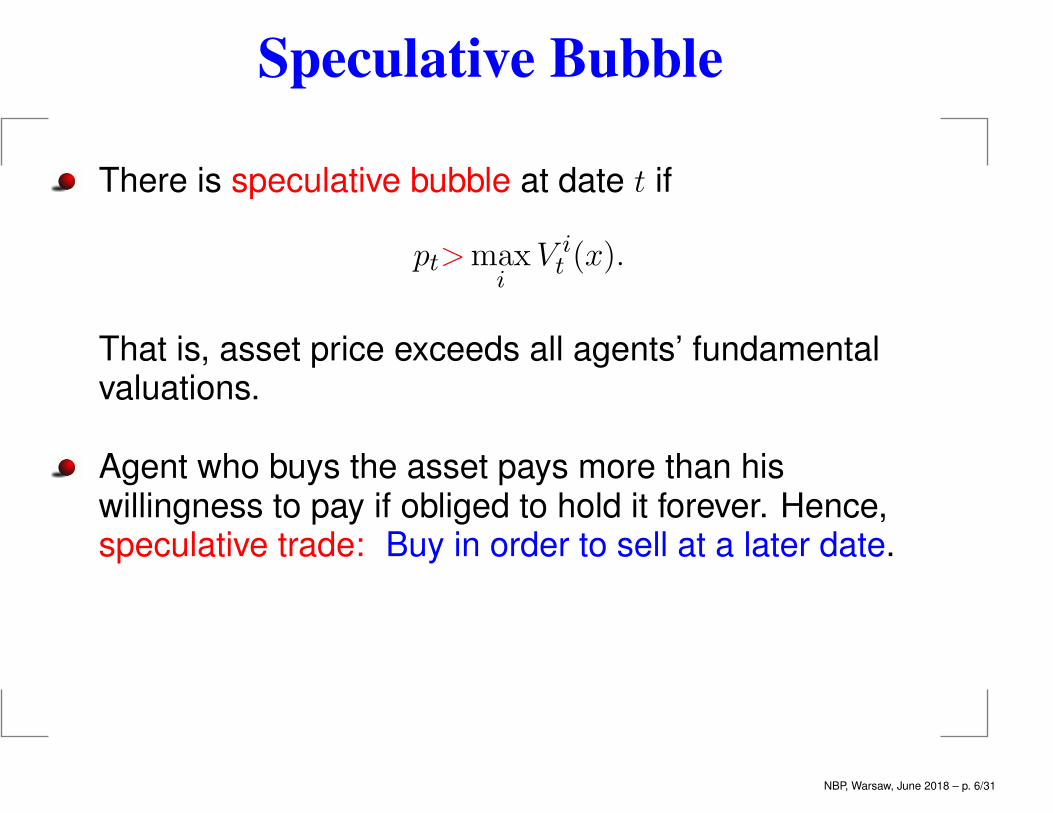
There is speculative bubble at date t if

pt>maxi

V it (x).

That is, asset price exceeds all agents’ fundamentalvaluations.

Agent who buys the asset pays more than hiswillingness to pay if obliged to hold it forever. Hence,speculative trade: Buy in order to sell at a later date.


Heterogeneous Beliefs

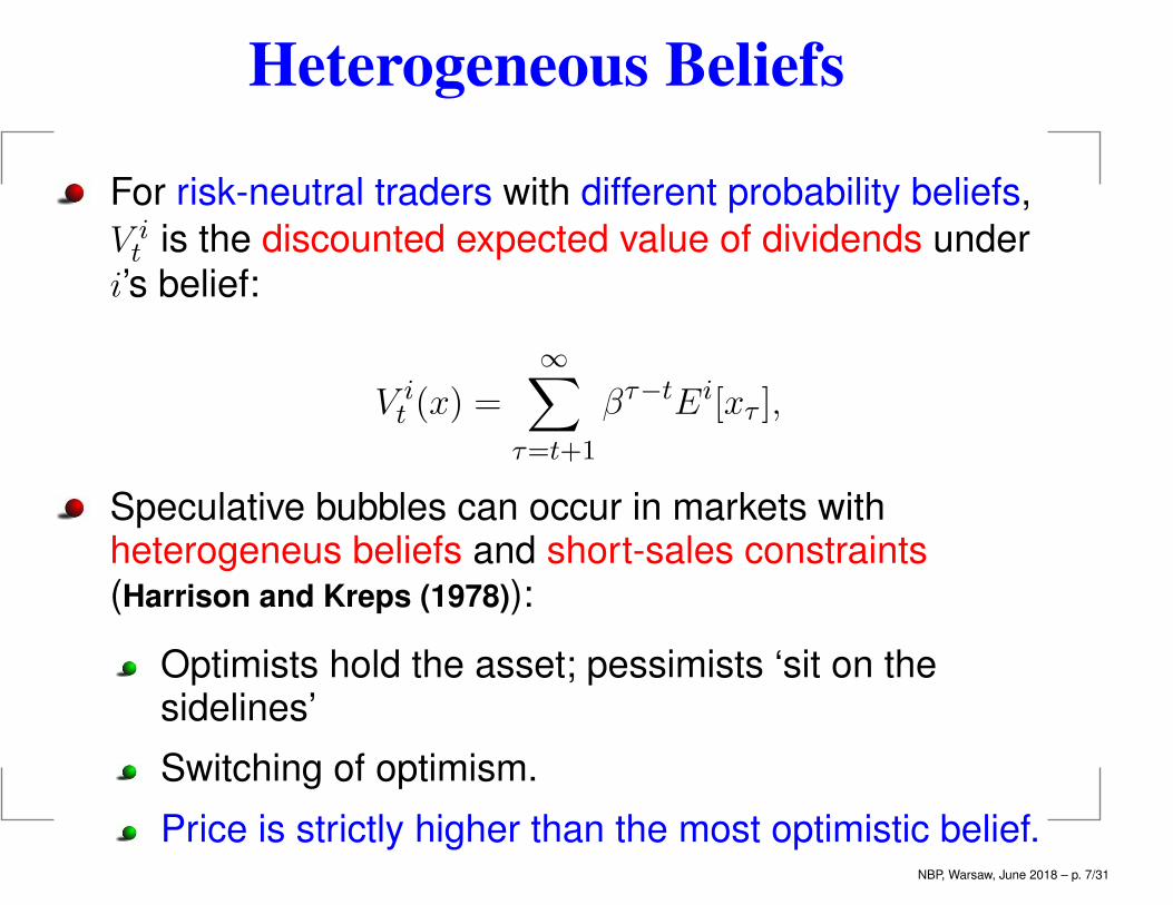
For risk-neutral traders with different probability beliefs,

V it is the discounted expected value of dividends under

i’s belief:

V it (x) =

∞∑τ=t+1

βτ−tEi[xτ ],

Speculative bubbles can occur in markets withheterogeneus beliefs and short-sales constraints(Harrison and Kreps (1978)):

Optimists hold the asset; pessimists ‘sit on thesidelines’

Switching of optimism.

Price is strictly higher than the most optimistic belief.NBP, Warsaw, June 2018 – p. 7/31

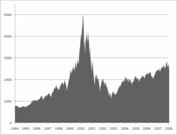
Dot.com Bubble

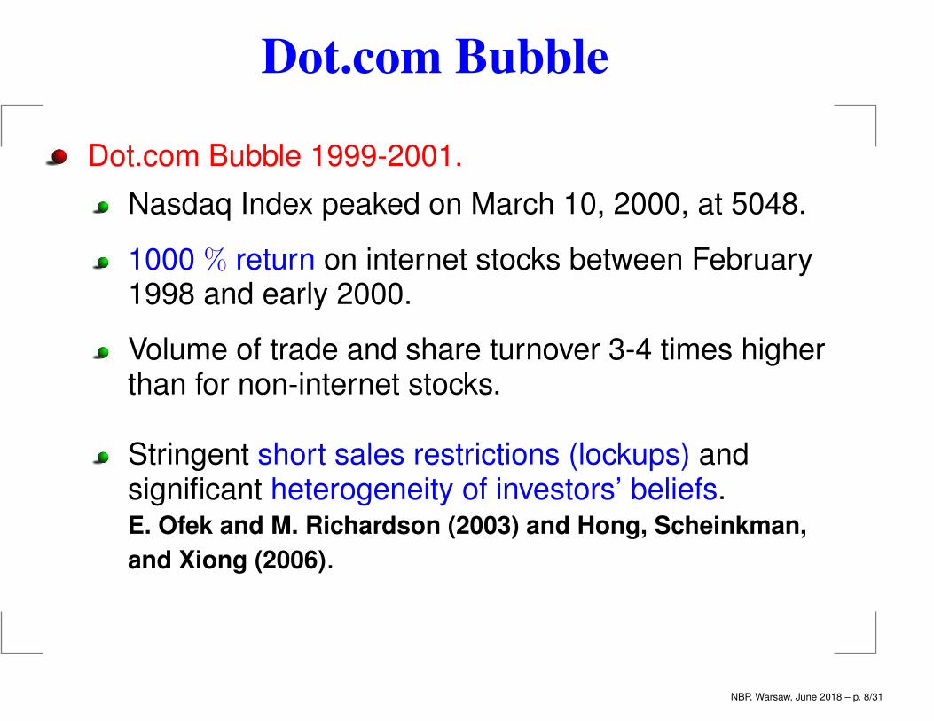
Dot.com Bubble 1999-2001.

Nasdaq Index peaked on March 10, 2000, at 5048.

1000 % return on internet stocks between February1998 and early 2000.

Volume of trade and share turnover 3-4 times higherthan for non-internet stocks.

Stringent short sales restrictions (lockups) andsignificant heterogeneity of investors’ beliefs.E. Ofek and M. Richardson (2003) and Hong, Scheinkman,

and Xiong (2006).


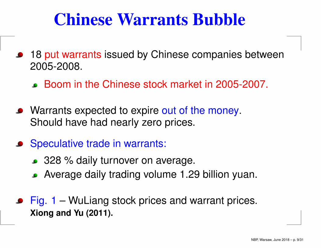
Chinese Warrants Bubble

18 put warrants issued by Chinese companies between2005-2008.

Boom in the Chinese stock market in 2005-2007.

Warrants expected to expire out of the money.Should have had nearly zero prices.

Speculative trade in warrants:

328 % daily turnover on average.

Average daily trading volume 1.29 billion yuan.

Fig. 1 – WuLiang stock prices and warrant prices.Xiong and Yu (2011).


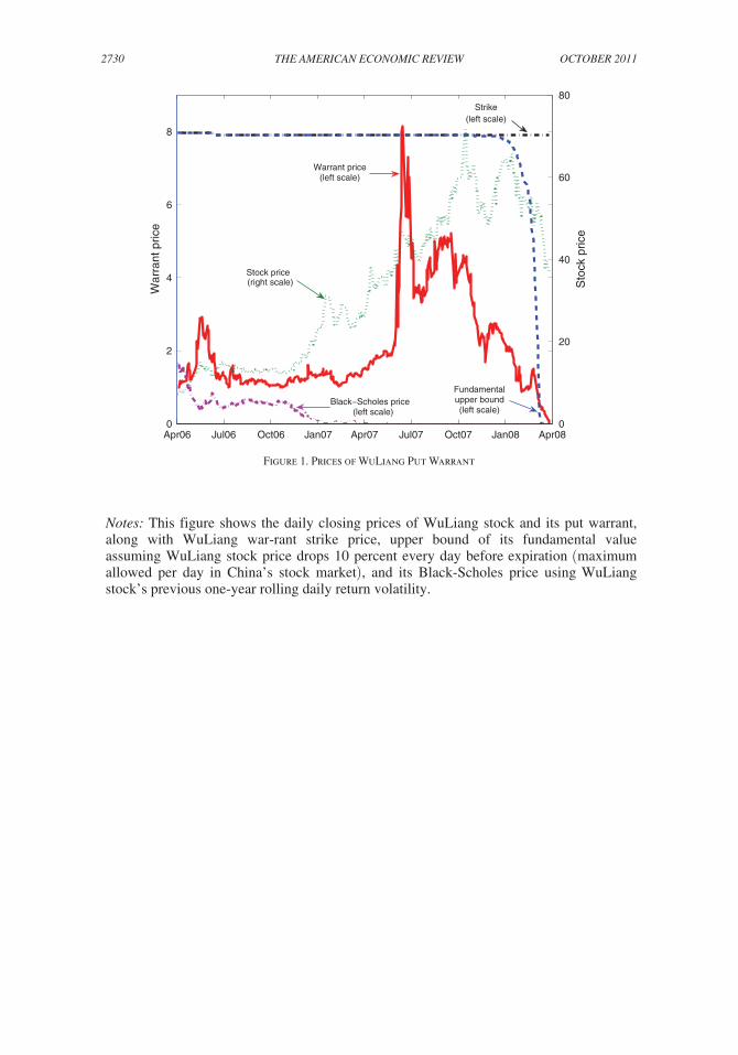
2730 THE AMERICAN ECONOMIC REVIEW OCTOBER 2011

Figure 1. Prices of WuLiang Put Warrant

Notes: This figure shows the daily closing prices of WuLiang stock and its put warrant, along with WuLiang war-rant strike price, upper bound of its fundamental value assuming WuLiang stock price drops 10 percent every day before expiration (maximum allowed per day in China’s stock market), and its Black-Scholes price using WuLiang stock’s previous one-year rolling daily return volatility.

Apr06 Jul06 Oct06 Jan07 Apr07 Jul07 Oct07 Jan08 Apr080

2

4

6

8

War

rant

pric

e

0

20

40

60

80

Sto

ck p

rice

Strike(left scale)

Stock price(right scale)

Fundamentalupper bound(left scale)

Warrant price(left scale)

Black−Scholes price(left scale)

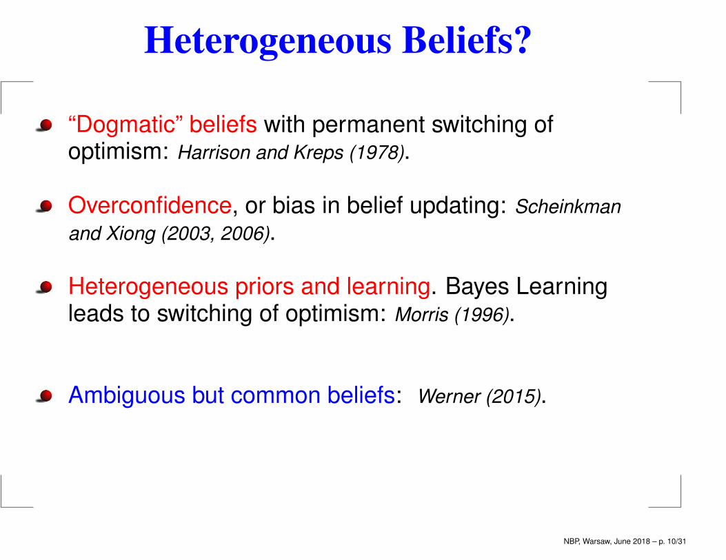
Heterogeneous Beliefs?

“Dogmatic” beliefs with permanent switching ofoptimism: Harrison and Kreps (1978).

Overconfidence, or bias in belief updating: Scheinkman

and Xiong (2003, 2006).

Heterogeneous priors and learning. Bayes Learningleads to switching of optimism: Morris (1996).

Ambiguous but common beliefs: Werner (2015).


Questions

Toward general theory of speculative bubbles:

When do heterogeneous beliefs give rise tospeculative trade and bubbles?

Bayesian learning and speculative bubbles.When do heterogeneous priors give rise tospeculative trade and bubbles?

Bayesian learning and the dynamics of pricebubbles.


Literature

Key references:

Harrison and Kreps (1978), Morris (1996).

Also Miller (1977), Scheinkman and Xiong (2003,2006), Harris and Raviv (1993), Slawski (2009).

Werner (2015)


Outline

Outline:

1. Valuation Switching and Speculative Bubbles.

2. Speculative Trade with Learning.

3. Example.

4. Merging of Beliefs and Disapperance of Bubbles.


Asset Market with no Short-Selling.

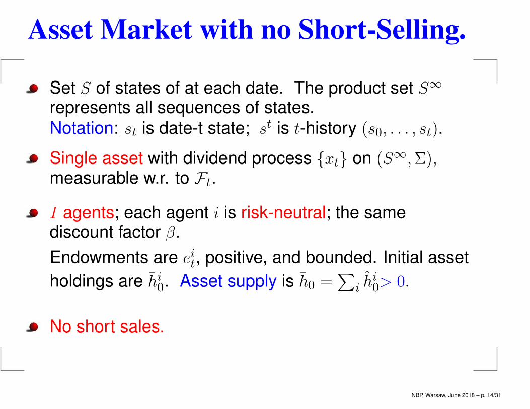
Set S of states of at each date. The product set S∞

represents all sequences of states.

Notation: st is date-t state; st is t-history (s0, . . . , st).

Single asset with dividend process {xt} on (S∞,Σ),measurable w.r. to Ft.

I agents; each agent i is risk-neutral; the samediscount factor β.

Endowments are eit, positive, and bounded. Initial asset

holdings are hi0. Asset supply is h0 =∑

i hi0> 0.

No short sales.


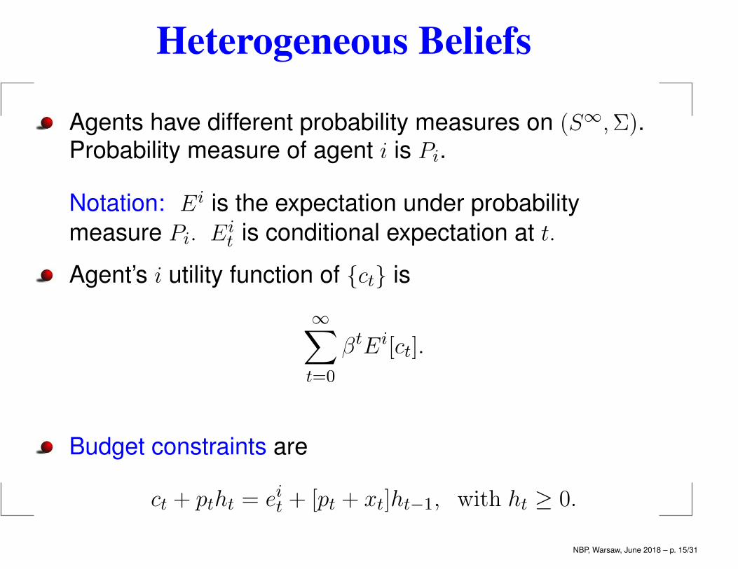
Heterogeneous Beliefs

Agents have different probability measures on (S∞,Σ).Probability measure of agent i is Pi.

Notation: Ei is the expectation under probability

measure Pi. Eit is conditional expectation at t.

Agent’s i utility function of {ct} is

∞∑t=0

βtEi[ct].

Budget constraints are

ct + ptht = eit + [pt + xt]ht−1, with ht ≥ 0.


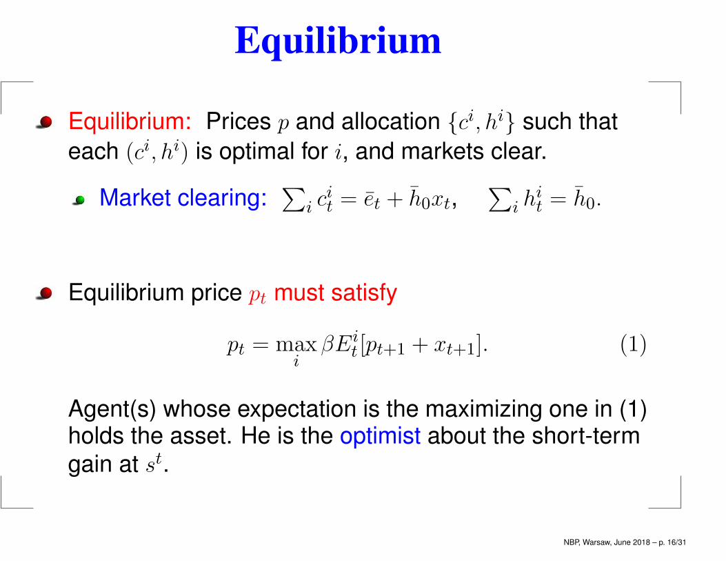
Equilibrium

Equilibrium: Prices p and allocation {ci, hi} such that

each (ci, hi) is optimal for i, and markets clear.

Market clearing:∑

i cit = et + h0xt,

∑i h

it = h0.

Equilibrium price pt must satisfy

pt = maxi

βEit [pt+1 + xt+1]. (1)

Agent(s) whose expectation is the maximizing one in (1)holds the asset. He is the optimist about the short-term

gain at st.


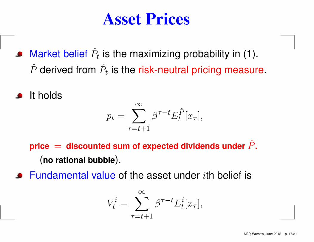
Asset Prices

Market belief Pt is the maximizing probability in (1).

P derived from Pt is the risk-neutral pricing measure.

It holds

pt =

∞∑τ=t+1

βτ−tEPt [xτ ],

price = discounted sum of expected dividends under P .

(no rational bubble).

Fundamental value of the asset under ith belief is

V it =

∞∑τ=t+1

βτ−tEit [xτ ],


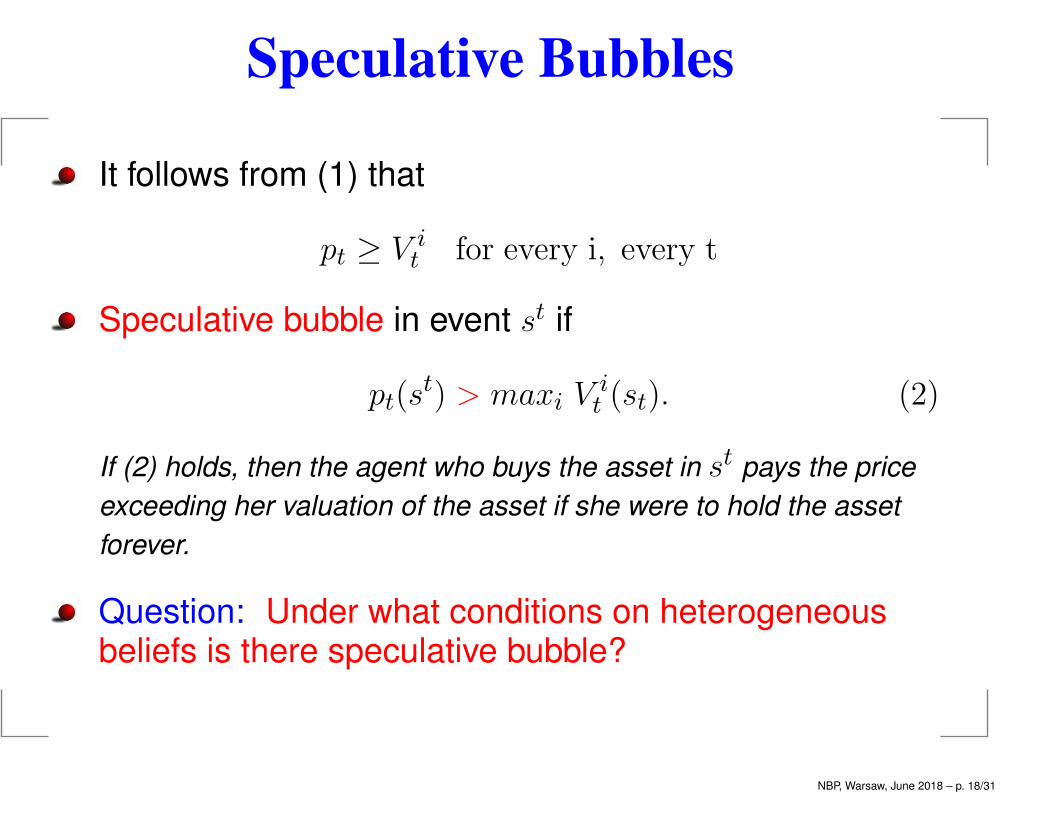
Speculative Bubbles

It follows from (1) that

pt ≥ V it for every i, every t

Speculative bubble in event st if

pt(st) > maxi V

it (st). (2)

If (2) holds, then the agent who buys the asset in st pays the price

exceeding her valuation of the asset if she were to hold the asset

forever.

Question: Under what conditions on heterogeneousbeliefs is there speculative bubble?


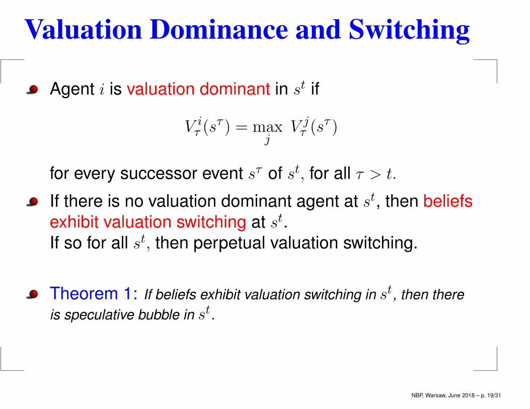
Valuation Dominance and Switching

Agent i is valuation dominant in st if

V iτ (s

τ ) = maxj

V jτ (s

τ )

for every successor event sτ of st, for all τ > t.

If there is no valuation dominant agent at st, then beliefs

exhibit valuation switching at st.

If so for all st, then perpetual valuation switching.

Theorem 1: If beliefs exhibit valuation switching in st, then there

is speculative bubble in st.


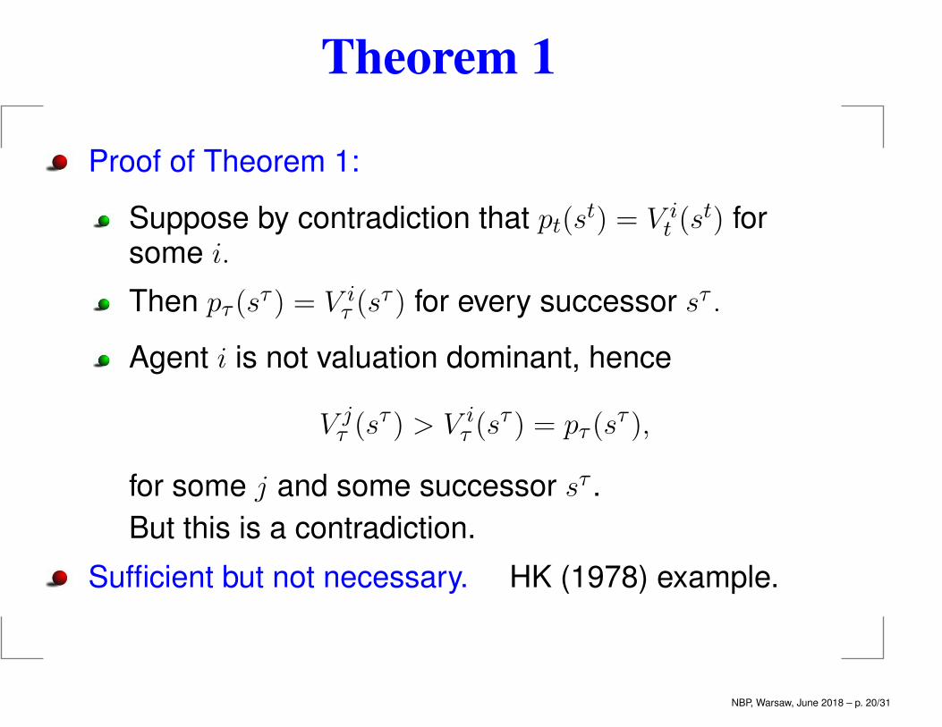
Theorem 1

Proof of Theorem 1:

Suppose by contradiction that pt(st) = V i

t (st) for

some i.

Then pτ (sτ ) = V i

τ (sτ ) for every successor sτ .

Agent i is not valuation dominant, hence

V jτ (s

τ ) > V iτ (s

τ ) = pτ (sτ ),

for some j and some successor sτ .

But this is a contradiction.

Sufficient but not necessary. HK (1978) example.


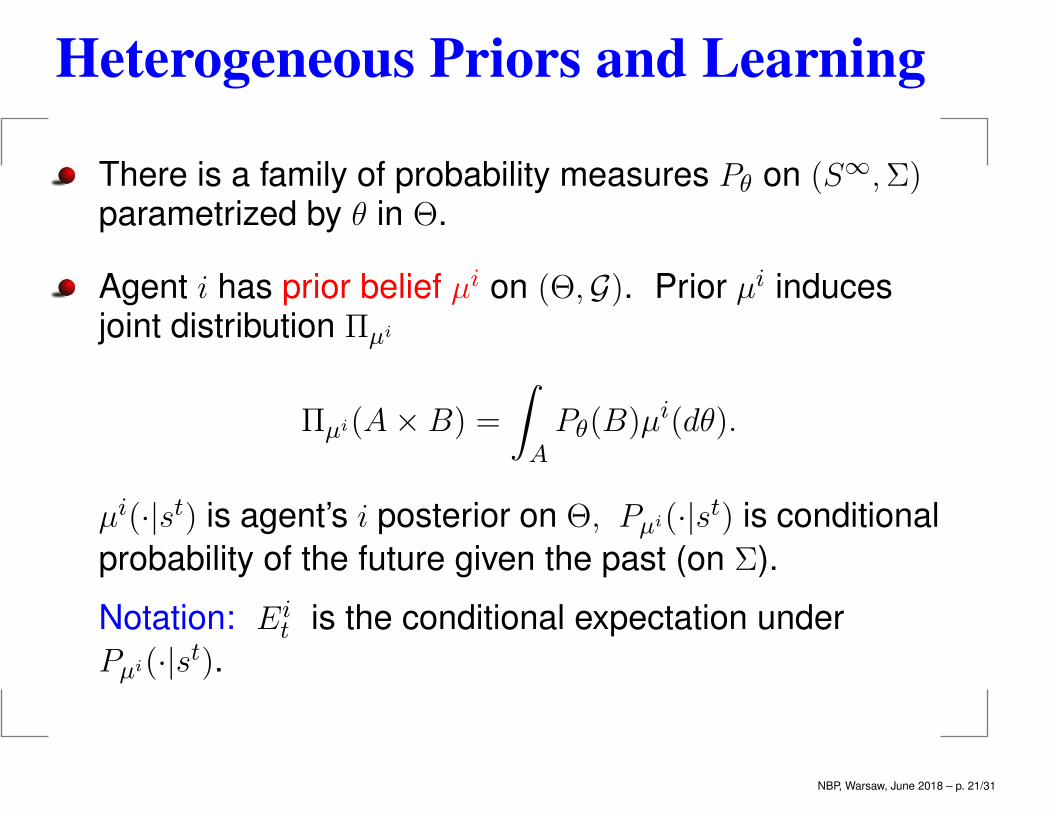
Heterogeneous Priors and Learning

There is a family of probability measures Pθ on (S∞,Σ)parametrized by θ in Θ.

Agent i has prior belief µi on (Θ,G). Prior µi inducesjoint distribution Πµi

Πµi(A× B) =

∫A

Pθ(B)µi(dθ).

µi(·|st) is agent’s i posterior on Θ, Pµi(·|st) is conditional

probability of the future given the past (on Σ).

Notation: Eit is the conditional expectation under

Pµi(·|st).


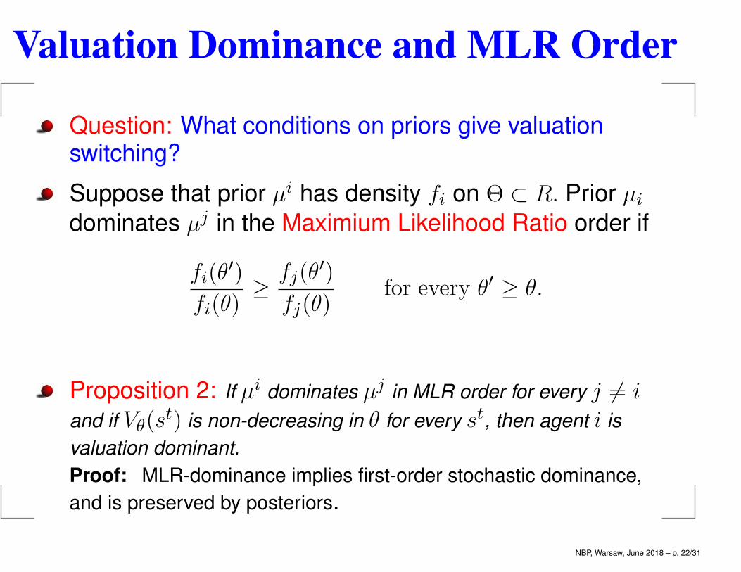
Valuation Dominance and MLR Order

Question: What conditions on priors give valuationswitching?

Suppose that prior µi has density fi on Θ ⊂ R. Prior µidominates µj in the Maximium Likelihood Ratio order if

fi(θ′)

fi(θ)≥ fj(θ

′)

fj(θ)for every θ′ ≥ θ.

Proposition 2: If µi dominates µj in MLR order for every j 6= iand if Vθ(s

t) is non-decreasing in θ for every st, then agent i is

valuation dominant.

Proof: MLR-dominance implies first-order stochastic dominance,

and is preserved by posteriors.


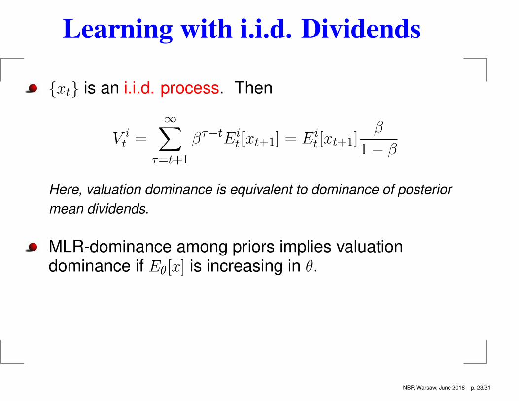
Learning with i.i.d. Dividends

{xt} is an i.i.d. process. Then

V it =

∞∑τ=t+1

βτ−tEit [xt+1] = Ei

t [xt+1]β

1− β

Here, valuation dominance is equivalent to dominance of posterior

mean dividends.

MLR-dominance among priors implies valuationdominance if Eθ[x] is increasing in θ.


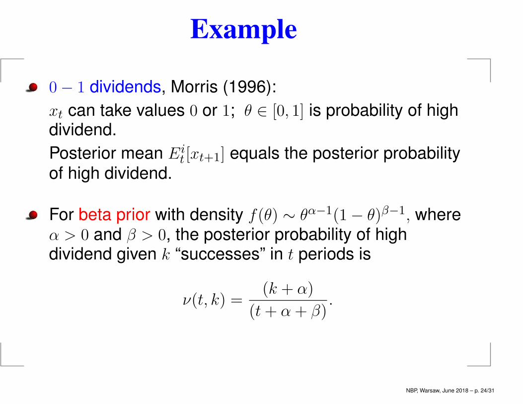
Example

0− 1 dividends, Morris (1996):

xt can take values 0 or 1; θ ∈ [0, 1] is probability of highdividend.

Posterior mean Eit [xt+1] equals the posterior probability

of high dividend.

For beta prior with density f(θ) ∼ θα−1(1− θ)β−1, whereα > 0 and β > 0, the posterior probability of highdividend given k “successes” in t periods is

ν(t, k) =(k + α)

(t+ α + β).


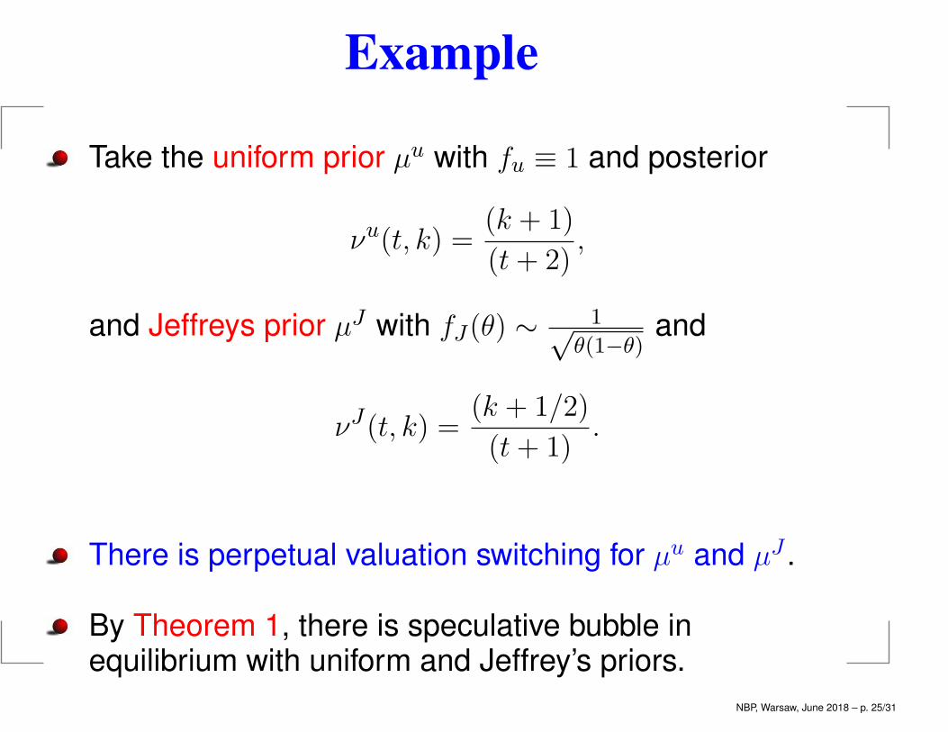
Example

Take the uniform prior µu with fu ≡ 1 and posterior

νu(t, k) =(k + 1)

(t+ 2),

and Jeffreys prior µJ with fJ(θ) ∼ 1√θ(1−θ)

and

νJ(t, k) =(k + 1/2)

(t+ 1).

There is perpetual valuation switching for µu and µJ .

By Theorem 1, there is speculative bubble inequilibrium with uniform and Jeffrey’s priors.


Example

More generally for beta priors, agent i is valuationdominant if and only if αi ≥ αj and βi ≤ βj for every j.

Valuation dominance is equivalent to the MonotoneLikelihood Ratio order for beta priors.


Merging of Beliefs and Bubbles

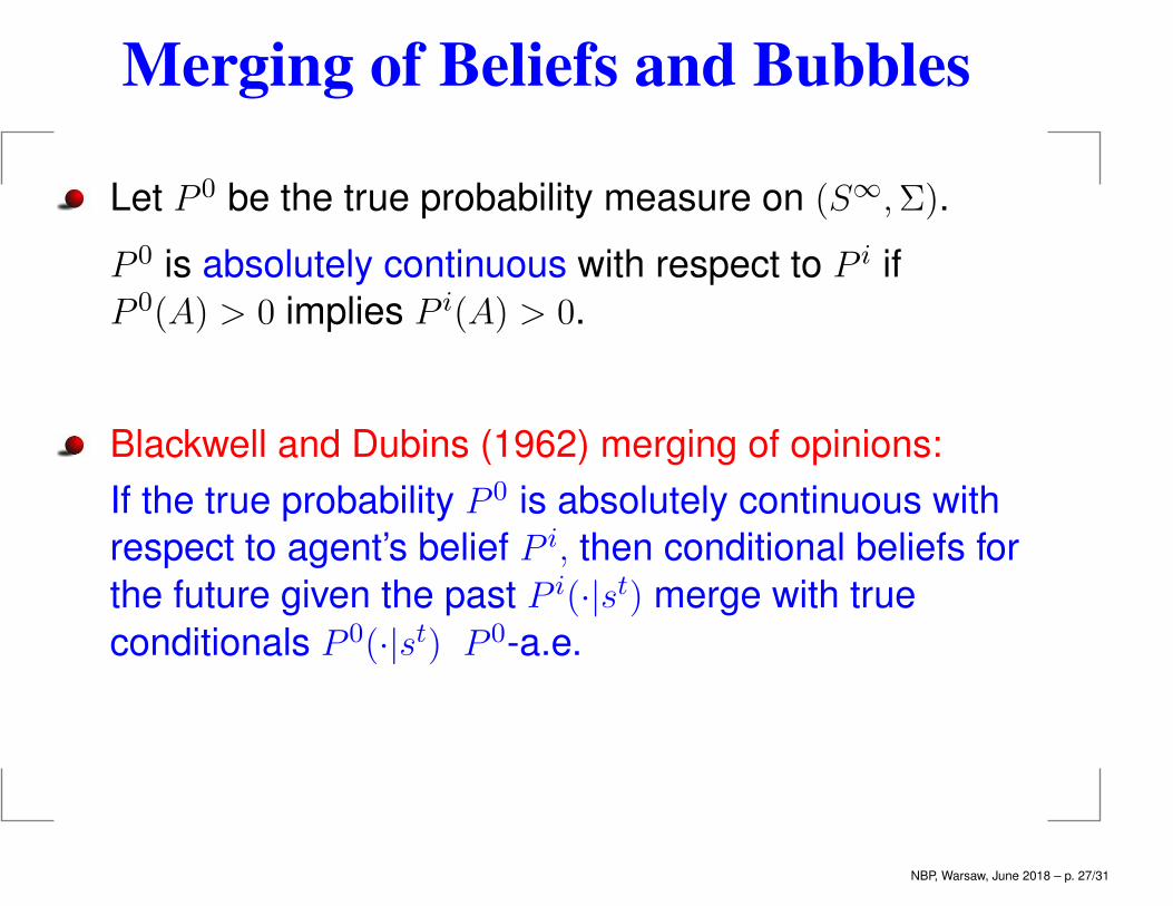
Let P 0 be the true probability measure on (S∞,Σ).

P 0 is absolutely continuous with respect to P i if

P 0(A) > 0 implies P i(A) > 0.

Blackwell and Dubins (1962) merging of opinions:

If the true probability P 0 is absolutely continuous with

respect to agent’s belief P i, then conditional beliefs for

the future given the past P i(·|st) merge with true

conditionals P 0(·|st) P 0-a.e.


Merging of Beliefs and Bubbles

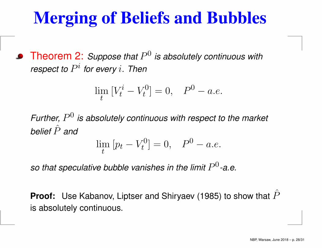
Theorem 2: Suppose that P 0 is absolutely continuous with

respect to P i for every i. Then

limt

[V it − V 0

t ] = 0, P 0 − a.e.

Further, P 0 is absolutely continuous with respect to the market

belief P and

limt

[pt − V 0t ] = 0, P 0 − a.e.

so that speculative bubble vanishes in the limit P 0-a.e.

Proof: Use Kabanov, Liptser and Shiryaev (1985) to show that Pis absolutely continuous.


Bayes Consistency and Bubbles

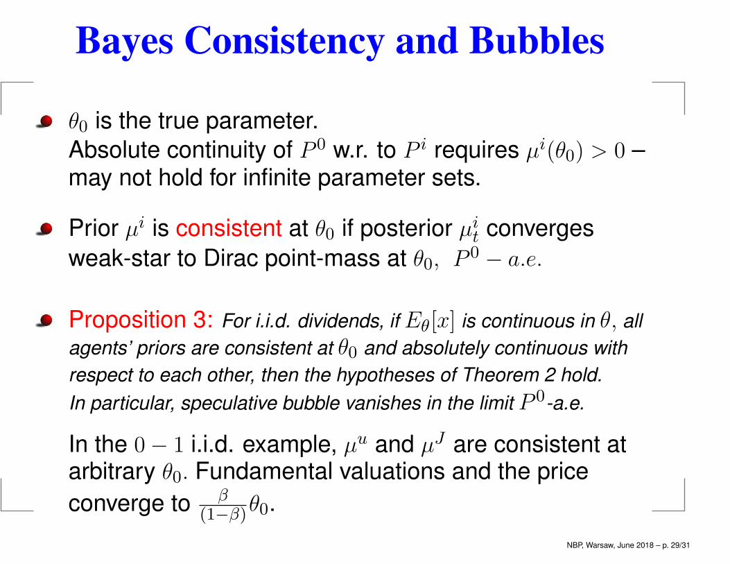
θ0 is the true parameter.

Absolute continuity of P 0 w.r. to P i requires µi(θ0) > 0 –may not hold for infinite parameter sets.

Prior µi is consistent at θ0 if posterior µit converges

weak-star to Dirac point-mass at θ0, P 0 − a.e.

Proposition 3: For i.i.d. dividends, if Eθ[x] is continuous in θ, all

agents’ priors are consistent at θ0 and absolutely continuous with

respect to each other, then the hypotheses of Theorem 2 hold.

In particular, speculative bubble vanishes in the limit P 0-a.e.

In the 0− 1 i.i.d. example, µu and µJ are consistent atarbitrary θ0. Fundamental valuations and the price

converge to β(1−β)θ0.


Bayes Consistency and Bubbles

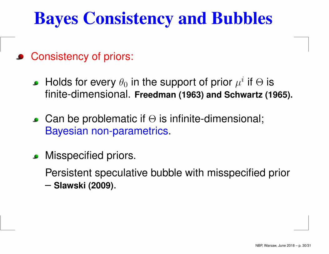
Consistency of priors:

Holds for every θ0 in the support of prior µi if Θ isfinite-dimensional. Freedman (1963) and Schwartz (1965).

Can be problematic if Θ is infinite-dimensional;Bayesian non-parametrics.

Misspecified priors.

Persistent speculative bubble with misspecified prior– Slawski (2009).


Conclusions

Speculative trade and bubbles are likely withheterogeneous priors and Bayes learning.

Bubbles may vanish in the long run, or be permanent.


speculative bubbles, heterogeneous beliefs, and … · speculative bubbles can occur in markets...

Documents