Speculators and Middlemen: The Role of Flippers in the Housing

Market

Patrick Bayer∗ Christopher Geissler† James W. Roberts‡

February 4, 2011

Abstract

In thinly traded markets for heterogenous, durable goods, such as housing, intermediariesmay play especially important roles. Using a unique micro-level dataset of housing transactionsin Los Angeles from 1988-2008 and a novel research design, we identify and measure the impor-tance of two very distinct types of intermediaries, also known as “flippers”. The first type actas middlemen who quickly match sellers and buyers, operate throughout housing market cyclesand earn above average returns when they buy and sell. The second type act as speculators whoattempt to time markets by holding assets for longer periods of time, perform relatively poorlywhen buying and selling and are strongly associated with price instability in their targeted areas.The presence of these unsophisticated speculators and positive feedback trading contribute thefirst pieces of evidence from the housing market to a growing body of work in other financialmarkets that questions whether speculators always act to stabilize prices.

JEL CODES: D82, D84, R30

Keywords: Speculation, Housing Markets, Asset Pricing, Behavioral Finance,Financial Intermediaries, Middlemen

∗Department of Economics, Duke University and NBER. Contact: patrick.bayer@duke.edu.†Department of Economics, Duke University. Contact: christopher.geissler@duke.edu.‡Department of Economics, Duke University. Contact: j.roberts@duke.edu.

1 Introduction

While housing assets constitute the majority of the wealth held by households in the United Statesand are subject to considerable volatility, research on the financial microstructure of the housingmarket has lagged that of the stock market by decades. While many influential papers on returns inthe stock market were written in the 1960s and 1970s, arguably the first systematic construction ofa return series for the housing market dates to the seminal paper by Case and Shiller (1989). In thepast several years, the kind of detailed transaction data used by Case and Shiller has become muchmore widely available, opening up a broad set of empirical finance questions related to housingmarkets.

Housing provides a prime example of a thin market for high value, durable goods. In suchmarkets, intermediaries often play a number of important economic roles. In housing markets,these intermediaries are often referred to as “flippers”, a term used to describe individuals or firmsthat buy homes with no intention to reside in or rent the property, but simply to quickly resell at aprofit. Flippers may serve as middlemen, purchasing from sellers with substantial holding costs whocannot afford to wait for the right buyer, thereby providing liquidity in this heterogeneous market.They may also make important physical investments in houses, if improvements are optimallymade when a house is empty or can be done by them at relatively low cost.1 And, they mayoperate as speculators, seeking to exploit arbitrage opportunities made possible through eithersuperior information about market fundamentals, or by exploiting deviations from the fundamentalsresulting from naıve decision-making on the part of other market actors.

Search frictions and cost asymmetries provide the impetus for flippers’ first two roles.2 Asfor the last role, modern finance theory describes a richer and more nuanced role for speculatorsthan just serving as the classic arbitrageurs of efficient markets theory, that instantly correct anydeviation in pricing from the fundamentals (e.g. Friedman (1953) and Fama (1955)). Some of thesources of rational investors’ hesitance to bet against asset mispricing include risk aversion and alack of close substitute investment opportunities (Wurgler and Zhuravskaya (2002)), noise traderrisk (De Long, Shleifer, Summers, and Waldmann (1990a)) and synchronization risk (Abreu andBrunnermeier (2002) and Abreu and Brunnermeier (2003)). A number of these features may bepresent in the housing market. For example, direct survey evidence showing that home-buyerstend to place excess weight on recent market trends when forming expectations of future priceappreciation (Case, Quigley, and Shiller (2003)) suggests a significant presence of noise traders inthe housing market.3 When homeowners chase trends in this way, i.e., engage in positive feedbacktrading, it can be optimal for rational speculators to jump on the bandwagon with them, buyingas prices begin to rise and selling out near the top of the bubble (De Long, Shleifer, Summers, and

1In this role, flippers may not only generate returns for themselves (if they can make these improvements atrelatively low cost), but may serve to maintain and restore the housing infrastructure of a community, leading topositive externalities in terms of house values and the local tax base for neighboring homeowners.

2See Spulber (1996), Rust and Hall (2003), and Hendershott and Zhang (2006), for example.3Evidence that homeowners may be subject to other behavioral biases such as loss aversion is shown in Genesove

and Mayer (2001) and Anenberg (2010).

2

Waldmann (1990b)). In this case, the actions of speculators work to fuel the bubble on the wayup and eventually dissolve it and help bring prices quickly back to the fundamentals on the waydown.4

Despite the potential importance of intermediaries, little is known about their activity or effecton this vital asset market. The goal of this paper is to identify the activity of flippers operating inthese three distinct economic roles and to study their impact on the housing market. Our analysisis based on comprehensive micro-level house transaction data from the Los Angeles metro areafrom 1988-2008 that allows us to identify flippers and study their activity. We introduce a novelresearch design to decompose observed returns on each flipped home into four components: (i) anydiscount on the transaction price at the time of purchase, (ii) any premium on the price at thetime of sale, (iii) market returns during the holding period, and (iv) any physical improvementsmade to the property by flippers. This last source of returns presents an econometric challenge forus since improvements are not directly observable in the data. It is here that our research designexploits the panel nature of the data to identify these components of the return. In particular, byexamining sales prices in transactions between pairs of non-flippers both prior to and following theperiod where a flipper buys and sells the property, we are able to control for any persistent changesin the houses unobservable quality that may have been due to flipper investment.

We establish that middlemen and speculators (i) follow very distinct strategies for when andwhere to buy and (ii) generate returns from almost completely distinct sources.5 Middlemen holdproperties for very short periods of time (a median of six months) and earn most of their return bybuying houses relatively cheaply. Flippers in this role tend to be professionals; the same individualsare observed transacting numerous properties throughout the sample period. Market timing is notan important source for their returns; they operate throughout booms and busts in the housingmarket and target neighborhoods that, if anything, are appreciating more slowly than the rest ofthe metro area.

By contrast, speculators tend to enter the housing market at an increasing rate as prices rise.They do not buy at much of a discount or sell at a premium, but instead earn almost their entirereturn through timing the market, i.e., earning the average market return. They operate only duringboom times and target neighborhoods with the highest expected price appreciation. Importantly,these targeted neighborhoods experience both an above average rate of appreciation in the shortterm (next 1-2 years) and a sharp decline in the intermediate term (3-5 years). In this way, entryby speculative flippers is strongly associated with the short-term amplification of neighborhoodhousing price cycles.

4Concerns that flippers may amplify fundamental cycles in local housing markets, thereby contributing to specu-lative bubbles, have given rise to recent legislation and regulatory changes by the federal government and a numberof states and localities seeking to limit flippers’ role in the market. For example, in 2006 HUD instituted a newregulation that made houses sold within 90 days of purchase ineligible for FHA financing.

5Although not the primary focus of the paper, our research design also enables us to measure the impact thatflippers have on the market through investment in physical home improvements. We estimate that flippers of bothtypes (speculators and middlemen) invest little more than the typical homeowner in their homes, implying that theirimpact on the market comes primarily from their roles in transacting and holding properties.

3

Interestingly, there are a number of signs that the real-world speculators that we identify in thedata may not be as sophisticated as the rational agents of finance theory. First, perhaps fueled byaccess to equity in their primary residence as prices rise, speculators tend to be amateurs that arenot particularly experienced at flipping houses. Secondly, many speculators continue to purchaseproperties at a rapid rate all the way up to the point that market reaches its peak and hold alarge fraction of their purchased properties well past the peak, thereby experiencing substantiallosses.6,7 Here, our paper is related to Brunnermeier and Nagel (2004) who examine the potentiallydestabilizing force of hedge funds during the technology bubble. While their findings suggest hedgefunds may be more sophisticated than our flippers (a fact which should not be terribly surprising),like their paper, ours too calls into question a central tenet of the efficient markets hypothesis: thatit is always optimal for rational speculators to attack a bubble.

Taken together, our analysis provides strong evidence that flippers play multiple economic rolesin the housing market. As middlemen, flippers may significantly enhance welfare by providingliquidity to high holding cost sellers. As investors in durable good quality, they may promoteneighborhood gentrification. Finally, as speculators, they are strongly associated with, and likelycontribute to, increased volatility in local housing markets, which has serious economic and socialconsequences. Given these roles’ dueling implications for welfare, and the fact that much of theiractivity occurs over short holding periods, it may be difficult and suboptimal to target flippers withanti-speculative policy prescriptions such as transaction taxes, which have been suggested in otherspeculative markets8, or by limiting their ability to finance investment.9

The paper proceeds as follows: Section 2 presents a simple theoretical discussion of the economicroles of flippers as middlemen and speculators. Section 3 describes the unique dataset used andthe definition of a flipper. Section 4 outlines the research design that will allow us to identifyflipper returns and investment. Section 5 gives our primary empirical results as well as robustnesschecks for these findings. Section 6 extends our analysis to the neighborhood level and focuses onwhat types of neighborhoods flippers target and their impact on these neighborhoods. Section 7investigates whether some flippers were caught holding houses when the housing market turned.Section 8 concludes.

6While our research design allows us to decompose the returns for a particular flipped house, it does not allowus to measure the returns to operating in the flipping business per se. In particular, because the same individualsthat flip certain properties may hold others for a very long time (presumably as rental units), the lack of informationon rents in our dataset precludes us from calculating returns for individual flippers. Moreover, our analysis providesonly an ex post estimate of the particular realization of returns for Los Angeles over the study period, rather than anex ante measure of expected returns. For these reasons, we confine the focus of our paper to a study of the behaviorand decomposition of the sources of returns for the distinct types of flippers described above.

7Whether the current boom and bust cycle was in fact a bubble in housing is a subject of intense debate. SeeHimmelberg, Mayer, and Sinai (2005) for a detailed discussion.

8See, for example, Tobin (1974), Tobin (1978), Eichengreen, Tobin, and Wyplosz (1995) or Summers and Summers(1988).

9A 2006 HUD regulation preventing FHA financing for houses sold within 90 days of purchase likely had this effect.More generally there is reason to believe a wave of “anti-flipper” sentiment may lead to further, similar legislation.

4

2 Motivating Model

To frame the empirical analysis, it is helpful to present some theoretical foundations for the potentialeconomic roles of flippers as middlemen and speculators. We begin by developing a simple modelof the role of flippers as middlemen, using it to explain why middlemen can profitably operate inboth hot and cold markets and to characterize how their returns are affected by market conditions.Drawing on the theoretical finance literature, we then describe a theoretical basis for the existenceof speculators in the housing market.

2.1 Flippers as Middlemen

We begin by developing a simple theoretical structure that captures the key elements of the homeselling problem. There are N potential sellers in each period and seller i has a per-period holdingcost hi ∼ F (h), with associated density f(h). In each period, sellers receive an offer with probabilityλ. Ordinary buyers make a take-it-or-leave-it offer drawn from a normal distribution N(µ, σ2). Aseller can accept the offer or reject it and wait until the next period to potentially sell the house toa new buyer. A maximum of one bidder visits the house in each period.

This structure captures the natural heterogeneity in holding costs and valuations that charac-terizes the housing market. Holding costs might be high, for example, if a seller needs to relocateto a new city or sell a house quickly to settle a divorce. They could be low if a family wants totrade up to a slightly larger house within the same city or neighborhood but still benefits from theconsumption value of their current house. Springer (1996) finds that distressed sellers deal morequickly and sell for less than other sellers. Glower, Haurin, and Hendershott (2003) find that whena seller takes a new job, he sells faster than average, indicating he likely has a higher holding cost.The offer probability λ captures how active or “hot” the market is, with higher values correspondingto more frequent offers.

The solution to the seller’s optimization problem can be summarized as the choice of a reserva-tion price, ri, which is the lowest acceptable offer. At the reservation price, the seller is indifferentbetween accepting and rejecting the offer. The reservation price takes the following form:

rit = E(oit|oit > rit)− hiE(tt|rit) (1)

where oit is the offer seller i receives at time t and tt is the time to sale from period t conditionalon not selling in period t. Given our assumption, time to sale follows a geometric distribution andin expectation is equal to (λt(1− Φ( rit−µσ )))−1. Equation 1 can therefore be rewritten as:

rit = µ+σφ

( rit−µσ

)1− Φ( rit−µσ )

− hi/λ

λt(1− Φ( rit−µσ ))(2)

The comparative statics of equation 2 are well-studied and it is straightforward to show thatthe reservation price is decreasing in hi and increasing in λ. That is, reservation prices will behigher when individuals have low holding costs and/or when the market is hot. Given that λ acts

5

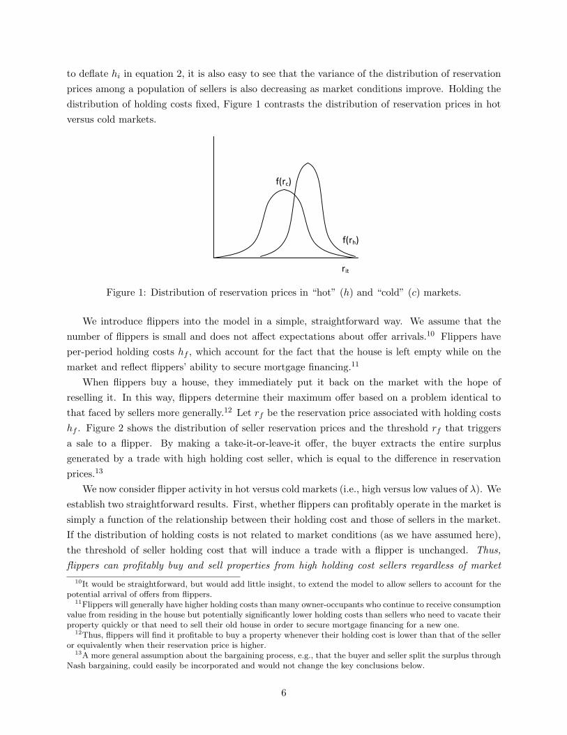
to deflate hi in equation 2, it is also easy to see that the variance of the distribution of reservationprices among a population of sellers is also decreasing as market conditions improve. Holding thedistribution of holding costs fixed, Figure 1 contrasts the distribution of reservation prices in hotversus cold markets.

!"#$$

$

$

$

$$$$$$$$

$$$

$

$$

$

%&!'($

($

$

$

!"#$

$$

$ $ $

$

($

%&!)($

($

%&!'($

($!"#$

%&!)($

($!"#$

!"#$

%&!'($

($

%&!)($

($!"#$

%&!)($

($

%&!'($

($

Figure 1: Distribution of reservation prices in “hot” (h) and “cold” (c) markets.

We introduce flippers into the model in a simple, straightforward way. We assume that thenumber of flippers is small and does not affect expectations about offer arrivals.10 Flippers haveper-period holding costs hf , which account for the fact that the house is left empty while on themarket and reflect flippers’ ability to secure mortgage financing.11

When flippers buy a house, they immediately put it back on the market with the hope ofreselling it. In this way, flippers determine their maximum offer based on a problem identical tothat faced by sellers more generally.12 Let rf be the reservation price associated with holding costshf . Figure 2 shows the distribution of seller reservation prices and the threshold rf that triggersa sale to a flipper. By making a take-it-or-leave-it offer, the buyer extracts the entire surplusgenerated by a trade with high holding cost seller, which is equal to the difference in reservationprices.13

We now consider flipper activity in hot versus cold markets (i.e., high versus low values of λ). Weestablish two straightforward results. First, whether flippers can profitably operate in the market issimply a function of the relationship between their holding cost and those of sellers in the market.If the distribution of holding costs is not related to market conditions (as we have assumed here),the threshold of seller holding cost that will induce a trade with a flipper is unchanged. Thus,flippers can profitably buy and sell properties from high holding cost sellers regardless of market

10It would be straightforward, but would add little insight, to extend the model to allow sellers to account for thepotential arrival of offers from flippers.

11Flippers will generally have higher holding costs than many owner-occupants who continue to receive consumptionvalue from residing in the house but potentially significantly lower holding costs than sellers who need to vacate theirproperty quickly or that need to sell their old house in order to secure mortgage financing for a new one.

12Thus, flippers will find it profitable to buy a property whenever their holding cost is lower than that of the selleror equivalently when their reservation price is higher.

13A more general assumption about the bargaining process, e.g., that the buyer and seller split the surplus throughNash bargaining, could easily be incorporated and would not change the key conclusions below.

6

!

!"

#$%"

&'()%"*")'()%*")'()%*"

&'()%"*"

%)%"" +,%"+,%"

&'()%"*"

&'()%"*"

%)%"" +,%"+,%"%)%""

)'()%*")'()%*"

%)%""

#)"

)'#$%*"

Figure 2: Distribution of seller reservation prices and the threshold rf triggering a sale to a flipper.

conditions.The second result that we establish is driven by the impact of market conditions on the distri-

bution of reservation prices. In particular, because reservation prices are more compressed in hotmarkets, the surplus generated by a transaction between a high holding cost seller and a flipperwill shrink, resulting in flippers paying higher prices relative to their own reservation values. Asa result, the “discount at purchase” that flippers receive at the time of purchase is smaller in hotversus cold markets.14

2.2 Flippers as Speculators

The theoretical finance literature supports (at least) two broad rationales for the existence ofspeculators in the housing market. Most obviously, efficient market theory admits an economic rolefor speculators that have access to better information than the broad set of agents participating in amarket. Given the decentralized nature of the housing market, with many individuals participatingin the home buying or selling process only a handful of times during their lives, it is easy toimagine that some market professionals might be especially well-informed or be able to processinformation in a sophisticated way that generates arbitrage opportunities. Under efficient marketstheory, acting on the basis of their superior information about the fundamentals, speculators havean unambiguously positive impact on the market, serving to align prices more closely with thefundamentals.

Behavioral finance theory admits a wider range of strategies for speculators and a much moreambiguous understanding of their impact on welfare and efficiency.15 The starting point for muchof modern behavioral finance theory is the presence of a set of naıve market actors, noise traders,who are subject to expectations and sentiments that are not fully justified by information aboutmarket fundamentals. By following simple strategies, such as chasing trends, or by sticking to rulesof thumb, noise traders can create distortions between prices and market fundamentals.

14Note that this does not imply that middlemen get lower average rates of return in hot versus cold markets, astheir time to sale will also be significantly shorter in hot market conditions.

15See Shleifer and Summers (1990), Barberis and Thaler (2003) and Shiller (2003) for excellent summaries ofstandard behavioral finance theory.

7

In this setting, potential arbitrageurs face multiple risks. Even if they are fully aware that priceshave temporarily deviated from the fundamentals, there is a risk that they might deviate further inthe short-run (depending on the beliefs and activity of the noise traders) before eventually fallingback in line with the fundamentals. It is not always optimal, therefore, for arbitrageurs to simply“go short” on any observed market deviations from the fundamentals.

In fact, it can be optimal to pursue a much wider range of strategies. If, for example, noisetraders engage in positive feedback trading - i.e., have a tendency to extrapolate or to chase thetrend, it can be optimal for rational speculators to jump on the bandwagon (De Long, Shleifer,Summers, and Waldmann (1990b)). By buying as noise traders begin to get interested in a market,speculators actually fuel the positive feedback trading that motivates the noise traders. And,by selling out as the market nears a peak, speculators speed the return of the market to thefundamentals. In this case, rational speculators take advantage of the noise traders by strategicallyselling out before the noise traders realize the bubble is about to burst. From this last example, itis easy to see that the welfare consequences of the existence of speculators need not be positive. Tothe extent that their actions fuel bubbles and increase volatility in the market, speculators tend todecrease welfare and market efficiency.

3 Data

The primary dataset for our analysis is based on a large database of housing transactions fromDataquick, a for profit company that collects publicly available information on houses and sellsthis information to interested businesses such as banks and lenders. For each transaction, the datacontain the names of the buyer and seller, the transaction price, the address and property identi-fication number, the transaction date, and numerous house characteristics including, for example,square footage, year built, number of bathrooms and bedrooms, lot size and whether the house hasa pool.

While these data are the most comprehensive available, there are some drawbacks to the wayDataquick creates its database. Dataquick collects information from two sources. Its transactionvariables, which include the date, price, and names of the buyer and seller are based on publiclyavailable data and thus cover every transaction in the United States. Its housing attribute vari-ables are drawn from a second public source, the local tax assessor’s office. The drawback is thatDataquick only maintains one assessor file, overwriting historical information, so that all observa-tions for a given house are essentially assigned the same house attributes. This prohibits researchersfrom tracking major home improvements by using changes in house characteristics over time. Giventhat these are the best data available, this drawback motivates our research design below in orderto track house improvements.

We focus on the five counties in the LA area (Los Angeles, Orange, Riverside, San Bernardino,and Ventura), between 1988 and 2008. From the initial set of transactions we clean the data forseveral reasons. We drop observations if we suspect that a property was split into several smaller

8

properties and resold, the price of the house was less than $1,16 the house sold more than once ina single day, the price or square footage was in the top or bottom one percent of the sample, thereis an inconsistency in the data such as the transaction year being earlier than the year the housewas built, or the sum of mortgages is $5,000 more than the house price. Table 1 provides summarystatistics of the cleaned data.

Mean Std. DevPrice 265,396 188,522Square Footage 1,598 607Transaction Year 1997.8 5.72Lotsize (sq. ft.) 10,871 601,047Year Built 1969.8 20.8Bathrooms 2.13 0.74Bedrooms 3.01 0.91Has Pool? 0.13 0.34Has Loan? 0.89 0.31Loan to Value 0.76 0.30Number of Transactions 2.35 1.23

Table 1: The table shows transaction-level summary statistics for data that cover five counties inthe LA area (Los Angeles, Orange, Riverside, San Bernardino, and Ventura). Based on 3,544,615transactions from 1988-2008. Loan to value and is measured relative to the price paid.

Anticipating our discussion of flipper behavior in “hot” and “cold” markets below, we summarizethe number of transactions over time in LA. We differentiate between hot and cold markets basedon transaction activity. As shown in Figure 3, LA was hot at the beginning of the sample periodand then cooled for most of the 1990s. In the late 1990s, it picked back up with sales peaking inthe 2002-2003 period before dropping significantly towards the end of the sample when the latesthousing boom collapsed.

3.1 Flippers

We identify flippers and flipped houses using two pieces of information in our dataset: the periodof time that a house was held and the names of buyers and sellers. We define a flipped house tobe one that satisfies three criteria: (1) the house must be bought and sold under the same namein less than two years;17 (2) the flipper must be an individual; and (3) the flipper must complete aminimum number of flips that satisfy (1).

The first criterion is motivated by our need to be able to measure returns. Not only do weneed to see the flipper buy and sell the house during the sample period but, because we do notobserve rental income, we focus on properties that are re-sold relatively quickly as these are likelyto be held empty during the holding period. Criterion (2) limits the sample to individuals instead

16A price of zero suggests that the seller did not put the house on the open market and instead transferred ownershipto a family member or friend. We are not interested in these transactions.

17In our robustness checks, we vary this length of time.

9

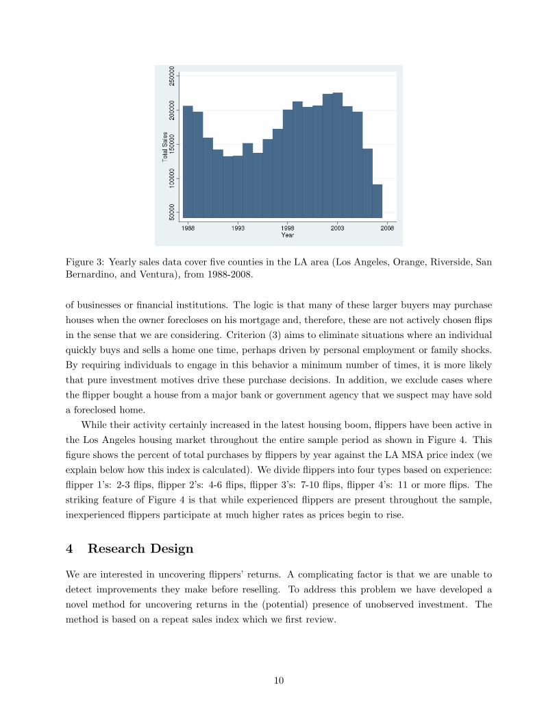
Figure 3: Yearly sales data cover five counties in the LA area (Los Angeles, Orange, Riverside, SanBernardino, and Ventura), from 1988-2008.

of businesses or financial institutions. The logic is that many of these larger buyers may purchasehouses when the owner forecloses on his mortgage and, therefore, these are not actively chosen flipsin the sense that we are considering. Criterion (3) aims to eliminate situations where an individualquickly buys and sells a home one time, perhaps driven by personal employment or family shocks.By requiring individuals to engage in this behavior a minimum number of times, it is more likelythat pure investment motives drive these purchase decisions. In addition, we exclude cases wherethe flipper bought a house from a major bank or government agency that we suspect may have solda foreclosed home.

While their activity certainly increased in the latest housing boom, flippers have been active inthe Los Angeles housing market throughout the entire sample period as shown in Figure 4. Thisfigure shows the percent of total purchases by flippers by year against the LA MSA price index (weexplain below how this index is calculated). We divide flippers into four types based on experience:flipper 1’s: 2-3 flips, flipper 2’s: 4-6 flips, flipper 3’s: 7-10 flips, flipper 4’s: 11 or more flips. Thestriking feature of Figure 4 is that while experienced flippers are present throughout the sample,inexperienced flippers participate at much higher rates as prices begin to rise.

4 Research Design

We are interested in uncovering flippers’ returns. A complicating factor is that we are unable todetect improvements they make before reselling. To address this problem we have developed anovel method for uncovering returns in the (potential) presence of unobserved investment. Themethod is based on a repeat sales index which we first review.

10

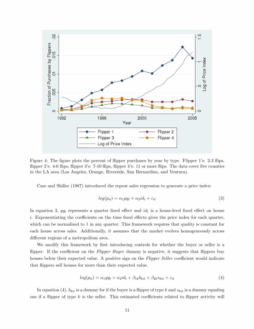
Figure 4: The figure plots the percent of flipper purchases by year by type. Flipper 1’s: 2-3 flips,flipper 2’s: 4-6 flips, flipper 3’s: 7-10 flips, flipper 4’s: 11 or more flips. The data cover five countiesin the LA area (Los Angeles, Orange, Riverside, San Bernardino, and Ventura).

Case and Shiller (1987) introduced the repeat sales regression to generate a price index:

log(pit) = α1yqt + α2idi + εit (3)

In equation 3, yqt represents a quarter fixed effect and idi is a house-level fixed effect on housei. Exponentiating the coefficients on the time fixed effects gives the price index for each quarter,which can be normalized to 1 in any quarter. This framework requires that quality is constant foreach house across sales. Additionally, it assumes that the market evolves homogeneously acrossdifferent regions of a metropolitan area.

We modify this framework by first introducing controls for whether the buyer or seller is aflipper. If the coefficient on the Flipper Buyer dummy is negative, it suggests that flippers buyhouses below their expected value. A positive sign on the Flipper Seller coefficient would indicatethat flippers sell houses for more than their expected value.

log(pit) = α1yqt + α2idi + β1kbkit + β2kskit + εit (4)

In equation (4), bkit is a dummy for if the buyer is a flipper of type k and skit is a dummy equalingone if a flipper of type k is the seller. This estimated coefficients related to flipper activity will

11

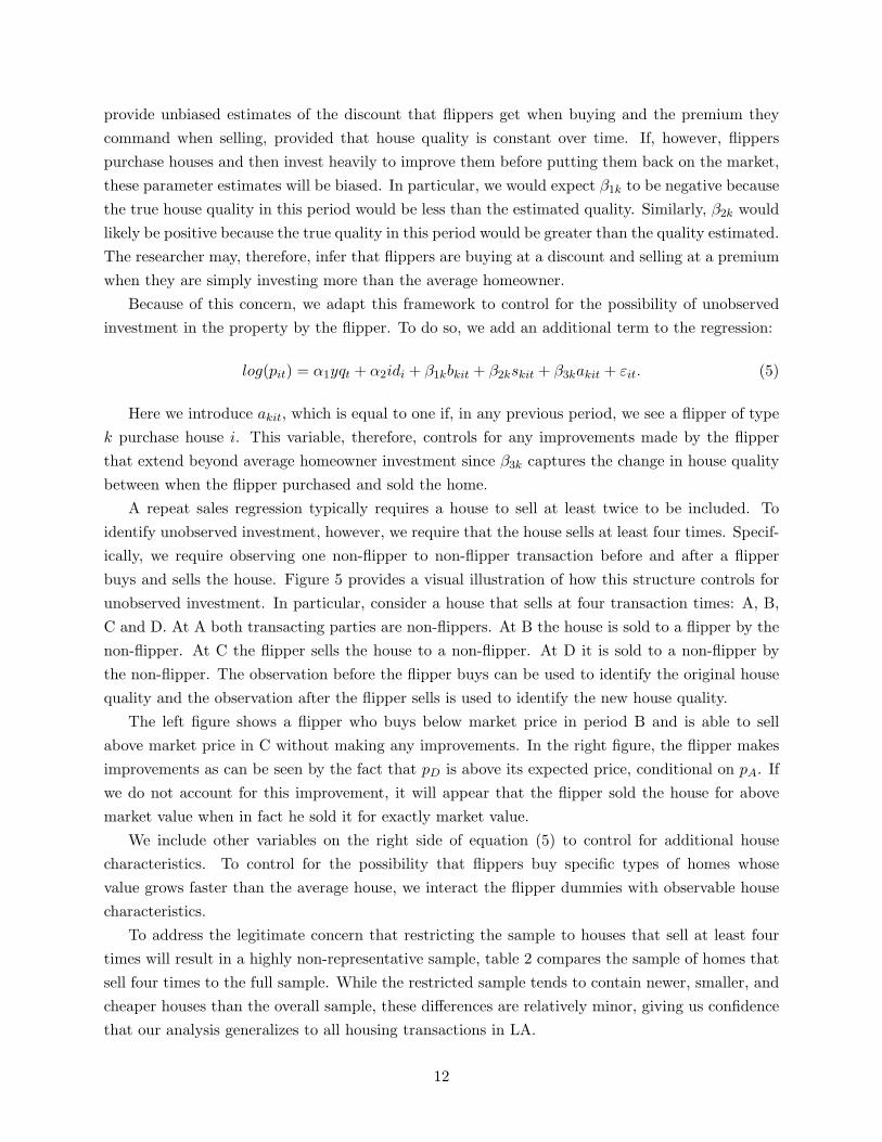
provide unbiased estimates of the discount that flippers get when buying and the premium theycommand when selling, provided that house quality is constant over time. If, however, flipperspurchase houses and then invest heavily to improve them before putting them back on the market,these parameter estimates will be biased. In particular, we would expect β1k to be negative becausethe true house quality in this period would be less than the estimated quality. Similarly, β2k wouldlikely be positive because the true quality in this period would be greater than the quality estimated.The researcher may, therefore, infer that flippers are buying at a discount and selling at a premiumwhen they are simply investing more than the average homeowner.

Because of this concern, we adapt this framework to control for the possibility of unobservedinvestment in the property by the flipper. To do so, we add an additional term to the regression:

log(pit) = α1yqt + α2idi + β1kbkit + β2kskit + β3kakit + εit. (5)

Here we introduce akit, which is equal to one if, in any previous period, we see a flipper of typek purchase house i. This variable, therefore, controls for any improvements made by the flipperthat extend beyond average homeowner investment since β3k captures the change in house qualitybetween when the flipper purchased and sold the home.

A repeat sales regression typically requires a house to sell at least twice to be included. Toidentify unobserved investment, however, we require that the house sells at least four times. Specif-ically, we require observing one non-flipper to non-flipper transaction before and after a flipperbuys and sells the house. Figure 5 provides a visual illustration of how this structure controls forunobserved investment. In particular, consider a house that sells at four transaction times: A, B,C and D. At A both transacting parties are non-flippers. At B the house is sold to a flipper by thenon-flipper. At C the flipper sells the house to a non-flipper. At D it is sold to a non-flipper bythe non-flipper. The observation before the flipper buys can be used to identify the original housequality and the observation after the flipper sells is used to identify the new house quality.

The left figure shows a flipper who buys below market price in period B and is able to sellabove market price in C without making any improvements. In the right figure, the flipper makesimprovements as can be seen by the fact that pD is above its expected price, conditional on pA. Ifwe do not account for this improvement, it will appear that the flipper sold the house for abovemarket value when in fact he sold it for exactly market value.

We include other variables on the right side of equation (5) to control for additional housecharacteristics. To control for the possibility that flippers buy specific types of homes whosevalue grows faster than the average house, we interact the flipper dummies with observable housecharacteristics.

To address the legitimate concern that restricting the sample to houses that sell at least fourtimes will result in a highly non-representative sample, table 2 compares the sample of homes thatsell four times to the full sample. While the restricted sample tends to contain newer, smaller, andcheaper houses than the overall sample, these differences are relatively minor, giving us confidencethat our analysis generalizes to all housing transactions in LA.

12

! !

!"

#"

!"$"

#"

%"

!"$"

%"

!"$"

%"

$"

#"%"

&'()"

*+',)" *+',)"

*+',)"*+',)"

&'()"

&'()"&'()"

-.*/01"

*/0"

-.*/01"

2/-"3",&"

"

*/0" 2/-"3",&"

#"

45"6(*+52)()7&8"

45"6(*+52)()7&8"

6(*+52)()7&8"

6(*+52)()7&8"

Figure 5: Left: A case where the flipper did not make improvements between periods B and C.Right: An instance where the flipper did make improvements between B and C.

All Observations ≥4 SalesYear Built 1969.8 1972.6

(20.8) (19.6)Year Bought 1997.8 1999.7

(5.72) (5.28)Square Feet 1,598 1,480

(607) (555)Number of Bedrooms 3.01 2.79

(0.91) (0.89)Number of Bathrooms 2.13 2.12

(0.74) (0.71)N 3,544,615 247,341

Table 2: The table shows transaction-level summary statistics by number of sales for data thatcover five counties in the LA area (Los Angeles, Orange, Riverside, San Bernardino, and Ventura).Standard deviations in parentheses. Based on 3,544,615 transactions from 1988-2008.

Finally, there is some chance that we still misestimate housing improvements within this frame-work. If a flipper improves the home, sells it to someone under whom the investment depreciatesto the point where the investment has no impact on price when this new owner sells, we maymistakenly believe that the flipper made no investment. We can check for this bias by varying thetime between sales since we will be more likely to detect flipper investment the shorter is the timethat the person who purchased the home from the flipper holds it before reselling. We perform thisrobustness check in Section 5.3.

5 Two Types of Flippers

In this section we analyze returns over time and across flipper types to illustrate the (i) presenceof and (ii) differences between middlemen and speculative intermediaries.

13

5.1 Flippers’ returns

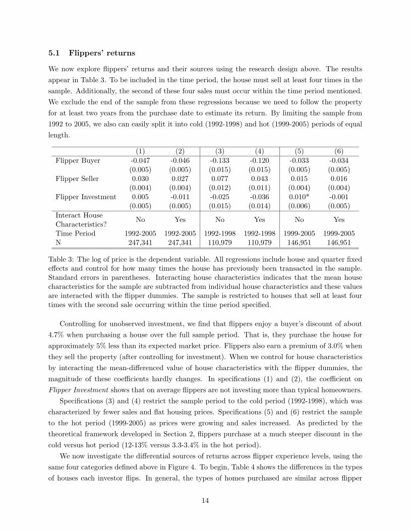
We now explore flippers’ returns and their sources using the research design above. The resultsappear in Table 3. To be included in the time period, the house must sell at least four times in thesample. Additionally, the second of these four sales must occur within the time period mentioned.We exclude the end of the sample from these regressions because we need to follow the propertyfor at least two years from the purchase date to estimate its return. By limiting the sample from1992 to 2005, we also can easily split it into cold (1992-1998) and hot (1999-2005) periods of equallength.

(1) (2) (3) (4) (5) (6)Flipper Buyer -0.047 -0.046 -0.133 -0.120 -0.033 -0.034

(0.005) (0.005) (0.015) (0.015) (0.005) (0.005)Flipper Seller 0.030 0.027 0.077 0.043 0.015 0.016

(0.004) (0.004) (0.012) (0.011) (0.004) (0.004)Flipper Investment 0.005 -0.011 -0.025 -0.036 0.010* -0.001

(0.005) (0.005) (0.015) (0.014) (0.006) (0.005)Interact HouseCharacteristics?

No Yes No Yes No Yes

Time Period 1992-2005 1992-2005 1992-1998 1992-1998 1999-2005 1999-2005N 247,341 247,341 110,979 110,979 146,951 146,951

Table 3: The log of price is the dependent variable. All regressions include house and quarter fixedeffects and control for how many times the house has previously been transacted in the sample.Standard errors in parentheses. Interacting house characteristics indicates that the mean housecharacteristics for the sample are subtracted from individual house characteristics and these valuesare interacted with the flipper dummies. The sample is restricted to houses that sell at least fourtimes with the second sale occurring within the time period specified.

Controlling for unobserved investment, we find that flippers enjoy a buyer’s discount of about4.7% when purchasing a house over the full sample period. That is, they purchase the house forapproximately 5% less than its expected market price. Flippers also earn a premium of 3.0% whenthey sell the property (after controlling for investment). When we control for house characteristicsby interacting the mean-differenced value of house characteristics with the flipper dummies, themagnitude of these coefficients hardly changes. In specifications (1) and (2), the coefficient onFlipper Investment shows that on average flippers are not investing more than typical homeowners.

Specifications (3) and (4) restrict the sample period to the cold period (1992-1998), which wascharacterized by fewer sales and flat housing prices. Specifications (5) and (6) restrict the sampleto the hot period (1999-2005) as prices were growing and sales increased. As predicted by thetheoretical framework developed in Section 2, flippers purchase at a much steeper discount in thecold versus hot period (12-13% versus 3.3-3.4% in the hot period).

We now investigate the differential sources of returns across flipper experience levels, using thesame four categories defined above in Figure 4. To begin, Table 4 shows the differences in the typesof houses each investor flips. In general, the types of homes purchased are similar across flipper

14

type except that more experienced flipper types tend to buy older homes.

Flipper Type 1 2 3 4 All HousesYear Built 1968.7 1963.2 1956.9 1953.7 1972.6

(22.0) (23.0) (23.1) (23.3) (19.6)Year Bought 2001.2 2000.7 2000.2 1999.3 1999.7

(2.70) (3.12) (3.19) (3.05) (5.28)Square Feet 1,467 1,380 1,295 1,275 1,480

(572) (513) (471) (436) (555)Number of Bedrooms 2.81 2.79 2.73 2.82 2.79

(1.00) (0.88) (0.88) (0.83) (0.89)Number of Bathrooms 2.05 1.96 1.79 1.70 2.12

(0.75) (0.73) (0.72) (0.68) (0.71)N 3,843 764 298 275 247,341

Table 4: The table shows house-level summary statistics by type of flipper for data that cover fivecounties in the LA area (Los Angeles, Orange, Riverside, San Bernardino, and Ventura). Standarddeviations in parentheses.

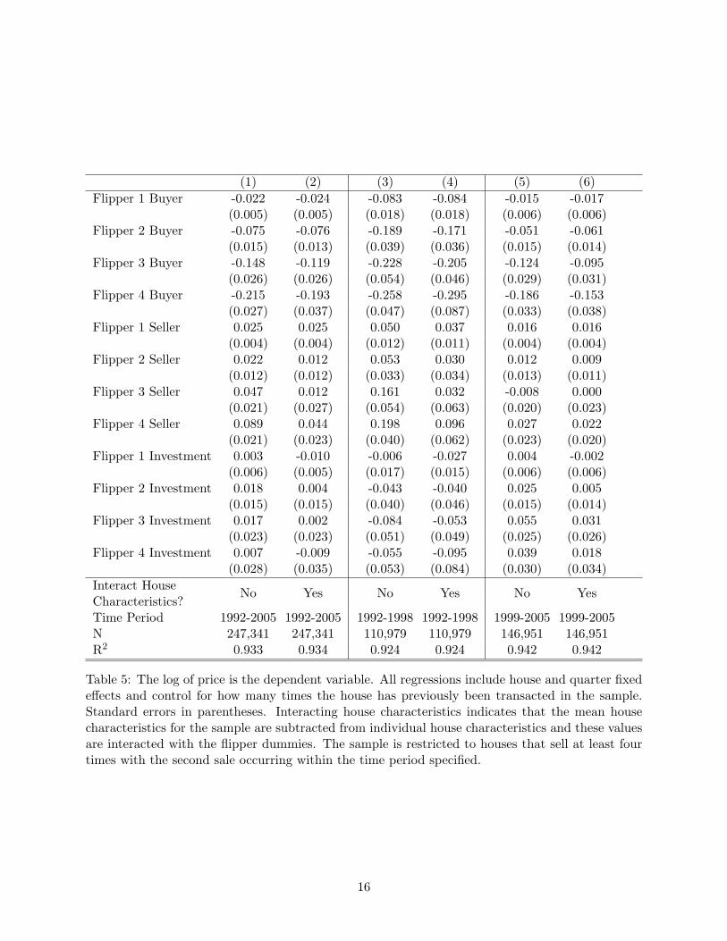
While it is clear that flippers outperform other market participants when both buying andselling (Table 3), there is distinct heterogeneity in this performance based on flipper experiencetype as Table 5 illustrates. Looking across flipper types, it is clear that while all flippers buyrelatively cheaply, more experienced flippers buy much more cheaply. There is also evidence thatflipper 4’s sell for relatively higher prices than do other flippers. Finally, even when controlling forflipper type, we still find that flippers invest very little in their houses prior to resale.

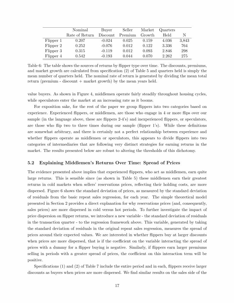
Using our repeat sales framework, we can also assess the composition of a flipper’s return:breaking this into a the fraction that stems from buying cheaply, selling high, and simply earningthe market return during the holding period. These results are in Table 6. We include estimates offlipper rates of return based on time held, market growth, and the residuals. These returns do notaccount for flippers’ transaction or holding costs, meaning actual returns are likely to be somewhatsmaller. Nonetheless, the estimated average rates of returns earned by all types of flippers duringour sample period suggest that they, in fact, can operate quite profitably in the market.

Table 6 highlights the distinction between flipper types and provides strong evidence that someflippers act as speculators while others operate as middlemen. First, there is a large disparity intime held. Flipper 4’s quickly resell their houses while flipper 1’s hold them almost twice as long.Second, flipper 1’s are not able to buy cheaply or sell for high prices and thus their (nominal) rateof return is primarily driven by overall market growth: 76% of their return stems from marketgrowth. Flipper 4’s, on the other hand, earn most of their return by purchasing well (purchasingcheaply generates 63% of their return) and quickly reselling so that only 21% of their return stemsfrom overall market growth. Taken together, these pieces of evidence clearly support the distinctionbetween middlemen and speculators in the market. Inexperienced flippers are speculators aimingto buy homes and hold on to them during times of overall market appreciation. Alternatively,middlemen aim to find homes they can buy at relatively large discounts and quickly resell to high

15

(1) (2) (3) (4) (5) (6)Flipper 1 Buyer -0.022 -0.024 -0.083 -0.084 -0.015 -0.017

(0.005) (0.005) (0.018) (0.018) (0.006) (0.006)Flipper 2 Buyer -0.075 -0.076 -0.189 -0.171 -0.051 -0.061

(0.015) (0.013) (0.039) (0.036) (0.015) (0.014)Flipper 3 Buyer -0.148 -0.119 -0.228 -0.205 -0.124 -0.095

(0.026) (0.026) (0.054) (0.046) (0.029) (0.031)Flipper 4 Buyer -0.215 -0.193 -0.258 -0.295 -0.186 -0.153

(0.027) (0.037) (0.047) (0.087) (0.033) (0.038)Flipper 1 Seller 0.025 0.025 0.050 0.037 0.016 0.016

(0.004) (0.004) (0.012) (0.011) (0.004) (0.004)Flipper 2 Seller 0.022 0.012 0.053 0.030 0.012 0.009

(0.012) (0.012) (0.033) (0.034) (0.013) (0.011)Flipper 3 Seller 0.047 0.012 0.161 0.032 -0.008 0.000

(0.021) (0.027) (0.054) (0.063) (0.020) (0.023)Flipper 4 Seller 0.089 0.044 0.198 0.096 0.027 0.022

(0.021) (0.023) (0.040) (0.062) (0.023) (0.020)Flipper 1 Investment 0.003 -0.010 -0.006 -0.027 0.004 -0.002

(0.006) (0.005) (0.017) (0.015) (0.006) (0.006)Flipper 2 Investment 0.018 0.004 -0.043 -0.040 0.025 0.005

(0.015) (0.015) (0.040) (0.046) (0.015) (0.014)Flipper 3 Investment 0.017 0.002 -0.084 -0.053 0.055 0.031

(0.023) (0.023) (0.051) (0.049) (0.025) (0.026)Flipper 4 Investment 0.007 -0.009 -0.055 -0.095 0.039 0.018

(0.028) (0.035) (0.053) (0.084) (0.030) (0.034)Interact HouseCharacteristics?

No Yes No Yes No Yes

Time Period 1992-2005 1992-2005 1992-1998 1992-1998 1999-2005 1999-2005N 247,341 247,341 110,979 110,979 146,951 146,951R2 0.933 0.934 0.924 0.924 0.942 0.942

Table 5: The log of price is the dependent variable. All regressions include house and quarter fixedeffects and control for how many times the house has previously been transacted in the sample.Standard errors in parentheses. Interacting house characteristics indicates that the mean housecharacteristics for the sample are subtracted from individual house characteristics and these valuesare interacted with the flipper dummies. The sample is restricted to houses that sell at least fourtimes with the second sale occurring within the time period specified.

16

Nominal Buyer Seller Market QuartersRate of Return Discount Premium Growth Held N

Flipper 1 0.207 -0.024 0.025 0.159 4.036 3,843Flipper 2 0.252 -0.076 0.012 0.122 3.336 764Flipper 3 0.315 -0.119 0.012 0.093 2.846 298Flipper 4 0.542 -0.193 0.044 0.070 2.262 275

Table 6: The table shows the sources of returns by flipper type over time. The discounts, premiums,and market growth are calculated from specification (2) of Table 5 and quarters held is simply themean number of quarters held. The nominal rate of return is generated by dividing the mean totalreturn (premium - discount + market growth) by the mean years held.

value buyers. As shown in Figure 4, middlemen operate fairly steadily throughout housing cycles,while speculators enter the market at an increasing rate as it booms.

For exposition sake, for the rest of the paper we group flippers into two categories based onexperience. Experienced flippers, or middlemen, are those who engage in 4 or more flips over oursample (in the language above, these are flippers 2-4’s) and inexperienced flippers, or speculators,are those who flip two to three times during our sample (flipper 1’s). While these definitionsare somewhat arbitrary, and there is certainly not a perfect relationship between experience andwhether flippers operate as middlemen or speculators, this appears to divide flippers into twocategories of intermediaries that are following very distinct strategies for earning returns in themarket. The results presented below are robust to altering the thresholds of this dichotomy.

5.2 Explaining Middlemen’s Returns Over Time: Spread of Prices

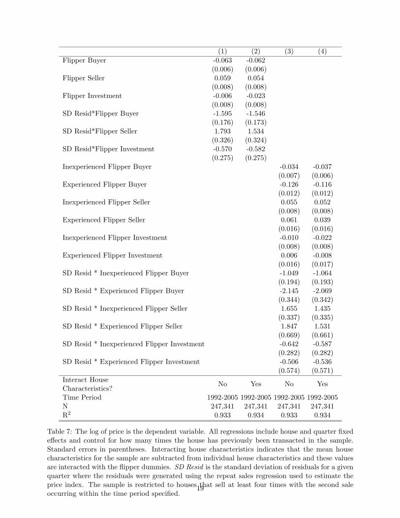
The evidence presented above implies that experienced flippers, who act as middlemen, earn quitelarge returns. This is sensible since (as shown in Table 5) these middlemen earn their greatestreturns in cold markets when sellers’ reservations prices, reflecting their holding costs, are moredispersed. Figure 6 shows the standard deviation of prices, as measured by the standard deviationof residuals from the basic repeat sales regression, for each year. The simple theoretical modelpresented in Section 2 provides a direct explanation for why reservations prices (and, consequently,sales prices) are more dispersed in cold versus hot periods. To further investigate the impact ofprice dispersion on flipper returns, we introduce a new variable - the standard deviation of residualsin the transaction quarter - to the regression framework above. This variable, generated by takingthe standard deviation of residuals in the original repeat sales regression, measures the spread ofprices around their expected values. We are interested in whether flippers buy at larger discountswhen prices are more dispersed, that is if the coefficient on the variable interacting the spread ofprices with a dummy for a flipper buying is negative. Similarly, if flippers earn larger premiumsselling in periods with a greater spread of prices, the coefficient on this interaction term will bepositive.

Specifications (1) and (2) of Table 7 include the entire period and in each, flippers receive largerdiscounts as buyers when prices are more dispersed. We find similar results on the sales side of the

17

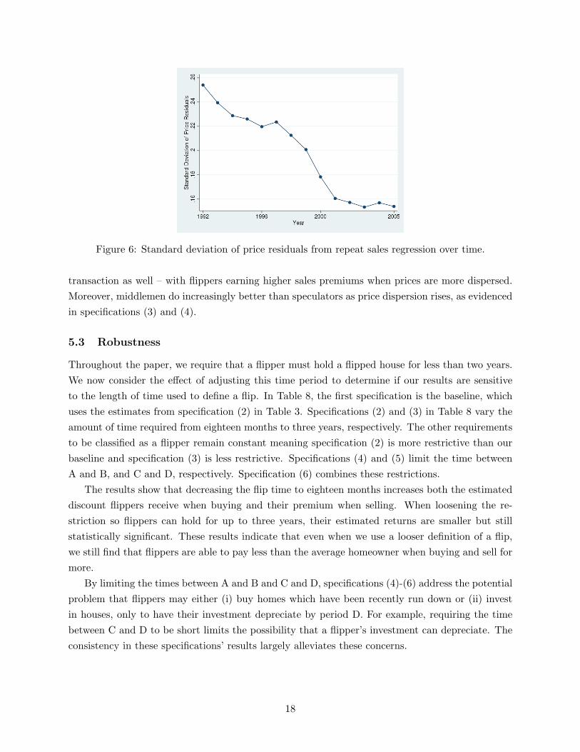
Figure 6: Standard deviation of price residuals from repeat sales regression over time.

transaction as well – with flippers earning higher sales premiums when prices are more dispersed.Moreover, middlemen do increasingly better than speculators as price dispersion rises, as evidencedin specifications (3) and (4).

5.3 Robustness

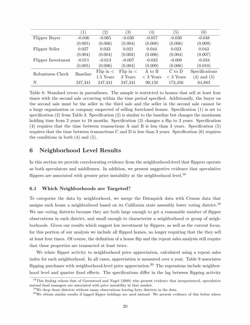
Throughout the paper, we require that a flipper must hold a flipped house for less than two years.We now consider the effect of adjusting this time period to determine if our results are sensitiveto the length of time used to define a flip. In Table 8, the first specification is the baseline, whichuses the estimates from specification (2) in Table 3. Specifications (2) and (3) in Table 8 vary theamount of time required from eighteen months to three years, respectively. The other requirementsto be classified as a flipper remain constant meaning specification (2) is more restrictive than ourbaseline and specification (3) is less restrictive. Specifications (4) and (5) limit the time betweenA and B, and C and D, respectively. Specification (6) combines these restrictions.

The results show that decreasing the flip time to eighteen months increases both the estimateddiscount flippers receive when buying and their premium when selling. When loosening the re-striction so flippers can hold for up to three years, their estimated returns are smaller but stillstatistically significant. These results indicate that even when we use a looser definition of a flip,we still find that flippers are able to pay less than the average homeowner when buying and sell formore.

By limiting the times between A and B and C and D, specifications (4)-(6) address the potentialproblem that flippers may either (i) buy homes which have been recently run down or (ii) investin houses, only to have their investment depreciate by period D. For example, requiring the timebetween C and D to be short limits the possibility that a flipper’s investment can depreciate. Theconsistency in these specifications’ results largely alleviates these concerns.

18

(1) (2) (3) (4)Flipper Buyer -0.063 -0.062

(0.006) (0.006)Flipper Seller 0.059 0.054

(0.008) (0.008)Flipper Investment -0.006 -0.023

(0.008) (0.008)SD Resid*Flipper Buyer -1.595 -1.546

(0.176) (0.173)SD Resid*Flipper Seller 1.793 1.534

(0.326) (0.324)SD Resid*Flipper Investment -0.570 -0.582

(0.275) (0.275)Inexperienced Flipper Buyer -0.034 -0.037

(0.007) (0.006)Experienced Flipper Buyer -0.126 -0.116

(0.012) (0.012)Inexperienced Flipper Seller 0.055 0.052

(0.008) (0.008)Experienced Flipper Seller 0.061 0.039

(0.016) (0.016)Inexperienced Flipper Investment -0.010 -0.022

(0.008) (0.008)Experienced Flipper Investment 0.006 -0.008

(0.016) (0.017)SD Resid * Inexperienced Flipper Buyer -1.049 -1.064

(0.194) (0.193)SD Resid * Experienced Flipper Buyer -2.145 -2.069

(0.344) (0.342)SD Resid * Inexperienced Flipper Seller 1.655 1.435

(0.337) (0.335)SD Resid * Experienced Flipper Seller 1.847 1.531

(0.669) (0.661)SD Resid * Inexperienced Flipper Investment -0.642 -0.587

(0.282) (0.282)SD Resid * Experienced Flipper Investment -0.506 -0.536

(0.574) (0.571)Interact HouseCharacteristics?

No Yes No Yes

Time Period 1992-2005 1992-2005 1992-2005 1992-2005N 247,341 247,341 247,341 247,341R2 0.933 0.934 0.933 0.934

Table 7: The log of price is the dependent variable. All regressions include house and quarter fixedeffects and control for how many times the house has previously been transacted in the sample.Standard errors in parentheses. Interacting house characteristics indicates that the mean housecharacteristics for the sample are subtracted from individual house characteristics and these valuesare interacted with the flipper dummies. SD Resid is the standard deviation of residuals for a givenquarter where the residuals were generated using the repeat sales regression used to estimate theprice index. The sample is restricted to houses that sell at least four times with the second saleoccurring within the time period specified.

19

(1) (2) (3) (4) (5) (6)Flipper Buyer -0.046 -0.065 -0.030 -0.057 -0.030 -0.048

(0.005) (0.006) (0.004) (0.008) (0.006) (0.009)Flipper Seller 0.027 0.033 0.021 0.044 0.023 0.043

(0.004) (0.004) (0.003) (0.006) (0.004) (0.007)Flipper Investment -0.011 -0.013 -0.007 -0.033 -0.008 -0.034

(0.005) (0.006) (0.004) (0.009) (0.006) (0.010)Flip in < Flip in < A to B C to D SpecificationsRobustness Check Baseline1.5 Years 3 Years < 3 Years < 3 Years (4) and (5)

N 247,341 247,341 247,341 90,150 173,456 64,883

Table 8: Standard errors in parentheses. The sample is restricted to houses that sell at least fourtimes with the second sale occurring within the time period specified. Additionally, the buyer onthe second sale must be the seller in the third sale and the seller in the second sale cannot bea large organization or company suspected of selling foreclosed homes. Specification (1) is set tospecification (2) from Table 3. Specification (2) is similar to the baseline but changes the maximumholding time from 2 years to 18 months. Specification (3) changes a flip to 3 years. Specification(4) requires that the time between transactions A and B is less than 3 years. Specification (5)requires that the time between transactions C and D is less than 3 years. Specification (6) requiresthe conditions in both (4) and (5).

6 Neighborhood Level Results

In this section we provide corroborating evidence from the neighborhood-level that flippers operateas both speculators and middlemen. In addition, we present suggestive evidence that speculativeflippers are associated with greater price instability at the neighborhood level.18

6.1 Which Neighborhoods are Targeted?

To categorize the data by neighborhood, we merge the Dataquick data with Census data thatassigns each house a neighborhood based on its California state assembly lower voting district.19

We use voting districts because they are both large enough to get a reasonable number of flipperobservations in each district, and small enough to characterize a neighborhood or group of neigh-borhoods. Given our results which suggest low investment by flippers, as well as the current focus,for this portion of our analysis we include all flipped homes, no longer requiring that the they sellat least four times. Of course, the definition of a house flip and the repeat sales analysis still requirethat these properties are transacted at least twice.

We relate flipper activity to neighborhood price appreciation, calculated using a repeat salesindex for each neighborhood. In all cases, appreciation is measured over a year. Table 9 associatesflipping purchases with neighborhood-level price appreciation.20 The regressions include neighbor-hood level and quarter fixed effects. The specifications differ in the lag between flipping activity

18This finding echoes that of Greenwood and Nagel (2009) who present evidence that inexperienced, speculativemutual fund managers are associated with price instability in that market.

19We drop those districts without many observations leaving forty districts in the data.20We obtain similar results if lagged flipper holdings are used instead. We present evidence of this below where

20

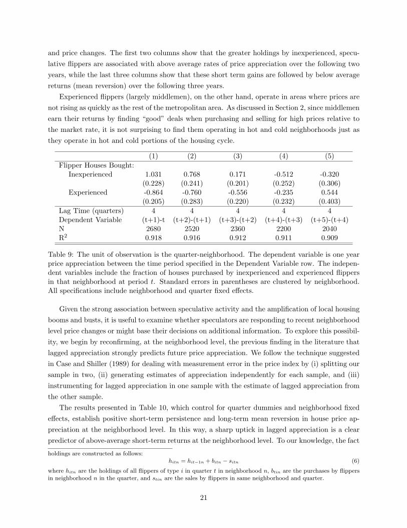
and price changes. The first two columns show that the greater holdings by inexperienced, specu-lative flippers are associated with above average rates of price appreciation over the following twoyears, while the last three columns show that these short term gains are followed by below averagereturns (mean reversion) over the following three years.

Experienced flippers (largely middlemen), on the other hand, operate in areas where prices arenot rising as quickly as the rest of the metropolitan area. As discussed in Section 2, since middlemenearn their returns by finding “good” deals when purchasing and selling for high prices relative tothe market rate, it is not surprising to find them operating in hot and cold neighborhoods just asthey operate in hot and cold portions of the housing cycle.

(1) (2) (3) (4) (5)Flipper Houses Bought:

Inexperienced 1.031 0.768 0.171 -0.512 -0.320(0.228) (0.241) (0.201) (0.252) (0.306)

Experienced -0.864 -0.760 -0.556 -0.235 0.544(0.205) (0.283) (0.220) (0.232) (0.403)

Lag Time (quarters) 4 4 4 4 4Dependent Variable (t+1)-t (t+2)-(t+1) (t+3)-(t+2) (t+4)-(t+3) (t+5)-(t+4)N 2680 2520 2360 2200 2040R2 0.918 0.916 0.912 0.911 0.909

Table 9: The unit of observation is the quarter-neighborhood. The dependent variable is one yearprice appreciation between the time period specified in the Dependent Variable row. The indepen-dent variables include the fraction of houses purchased by inexperienced and experienced flippersin that neighborhood at period t. Standard errors in parentheses are clustered by neighborhood.All specifications include neighborhood and quarter fixed effects.

Given the strong association between speculative activity and the amplification of local housingbooms and busts, it is useful to examine whether speculators are responding to recent neighborhoodlevel price changes or might base their decisions on additional information. To explore this possibil-ity, we begin by reconfirming, at the neighborhood level, the previous finding in the literature thatlagged appreciation strongly predicts future price appreciation. We follow the technique suggestedin Case and Shiller (1989) for dealing with measurement error in the price index by (i) splitting oursample in two, (ii) generating estimates of appreciation independently for each sample, and (iii)instrumenting for lagged appreciation in one sample with the estimate of lagged appreciation fromthe other sample.

The results presented in Table 10, which control for quarter dummies and neighborhood fixedeffects, establish positive short-term persistence and long-term mean reversion in house price ap-preciation at the neighborhood level. In this way, a sharp uptick in lagged appreciation is a clearpredictor of above-average short-term returns at the neighborhood level. To our knowledge, the fact

holdings are constructed as follows:hitn = hit−1n + bitn − sitn (6)

where hitn are the holdings of all flippers of type i in quarter t in neighborhood n, btin are the purchases by flippersin neighborhood n in the quarter, and stin are the sales by flippers in same neighborhood and quarter.

21

(1) (2) (3) (4) (5)Lagged Appreciation 0.453 0.104 -0.080 -0.198 -0.222

(0.061) (0.062) (0.076) (0.072) (0.100)Lag Time (quarters) 4 4 4 4 4Dependent Variable (t+1)-t (t+2)-(t+1) (t+3)-(t+2) (t+4)-(t+3) (t+5)-(t+4)N 2680 2520 2360 2200 2040R2 0.873 0.886 0.883 0.882 0.880

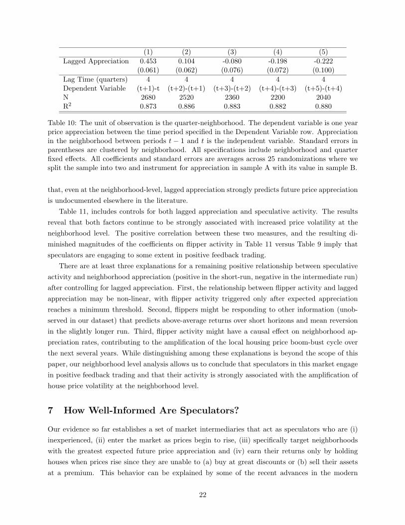
Table 10: The unit of observation is the quarter-neighborhood. The dependent variable is one yearprice appreciation between the time period specified in the Dependent Variable row. Appreciationin the neighborhood between periods t − 1 and t is the independent variable. Standard errors inparentheses are clustered by neighborhood. All specifications include neighborhood and quarterfixed effects. All coefficients and standard errors are averages across 25 randomizations where wesplit the sample into two and instrument for appreciation in sample A with its value in sample B.

that, even at the neighborhood-level, lagged appreciation strongly predicts future price appreciationis undocumented elsewhere in the literature.

Table 11, includes controls for both lagged appreciation and speculative activity. The resultsreveal that both factors continue to be strongly associated with increased price volatility at theneighborhood level. The positive correlation between these two measures, and the resulting di-minished magnitudes of the coefficients on flipper activity in Table 11 versus Table 9 imply thatspeculators are engaging to some extent in positive feedback trading.

There are at least three explanations for a remaining positive relationship between speculativeactivity and neighborhood appreciation (positive in the short-run, negative in the intermediate run)after controlling for lagged appreciation. First, the relationship between flipper activity and laggedappreciation may be non-linear, with flipper activity triggered only after expected appreciationreaches a minimum threshold. Second, flippers might be responding to other information (unob-served in our dataset) that predicts above-average returns over short horizons and mean reversionin the slightly longer run. Third, flipper activity might have a causal effect on neighborhood ap-preciation rates, contributing to the amplification of the local housing price boom-bust cycle overthe next several years. While distinguishing among these explanations is beyond the scope of thispaper, our neighborhood level analysis allows us to conclude that speculators in this market engagein positive feedback trading and that their activity is strongly associated with the amplification ofhouse price volatility at the neighborhood level.

7 How Well-Informed Are Speculators?

Our evidence so far establishes a set of market intermediaries that act as speculators who are (i)inexperienced, (ii) enter the market as prices begin to rise, (iii) specifically target neighborhoodswith the greatest expected future price appreciation and (iv) earn their returns only by holdinghouses when prices rise since they are unable to (a) buy at great discounts or (b) sell their assetsat a premium. This behavior can be explained by some of the recent advances in the modern

22

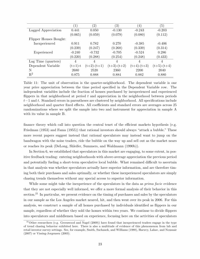
(1) (2) (3) (4) (5)Lagged Appreciation 0.441 0.050 -0.130 -0.243 -0.203

(0.065) (0.059) (0.079) (0.080) (0.112)Flipper Houses Bought:

Inexperienced 0.911 0.782 0.270 -0.385 -0.406(0.239) (0.247) (0.268) (0.339) (0.314)

Experienced -0.240 -0.732 -0.705 -0.524 0.286(0.220) (0.288) (0.254) (0.248) (0.433)

Lag Time (quarters) 4 4 4 4 4Dependent Variable (t+1)-t (t+2)-(t+1) (t+3)-(t+2) (t+4)-(t+3) (t+5)-(t+4)N 2680 2520 2360 2200 2040R2 0.875 0.888 0.884 0.882 0.880

Table 11: The unit of observation is the quarter-neighborhood. The dependent variable is oneyear price appreciation between the time period specified in the Dependent Variable row. Theindependent variables include the fraction of houses purchased by inexperienced and experiencedflippers in that neighborhood at period t and appreciation in the neighborhood between periodst−1 and t. Standard errors in parentheses are clustered by neighborhood. All specifications includeneighborhood and quarter fixed effects. All coefficients and standard errors are averages across 25randomizations where we split the sample into two and instrument for appreciation in sample Awith its value in sample B.

finance theory which call into question the central tenet of the efficient markets hypothesis (e.g.Friedman (1953) and Fama (1955)) that rational investors should always “attack a bubble.” Thesemore recent papers suggest instead that rational speculators may instead want to jump on thebandwagon with the noise traders, ride the bubble on the way up and sell out as the market nearsor reaches its peak (DeLong, Shleifer, Summers, and Waldmann (1990b)).

In Section 6, we established that speculators in this market are engaging, to some extent, in pos-itive feedback trading: entering neighborhoods with above-average appreciation the previous periodand potentially fueling a short-term speculative local bubble. What remained difficult to ascertainin that analysis was whether speculators actually have superior information, and are therefore tim-ing both their purchases and sales optimally, or whether these inexperienced speculators are simplychasing trends themselves without any special access to superior information.

While some might take the inexperience of the speculators in the data as prima facie evidencethat they are not especially well informed, we offer a more formal analysis of their behavior in thissection.21 In particular, we present evidence on the timing of purchases and sales by the speculatorsin our sample as the Los Angeles market neared, hit, and then went over its peak in 2006. For thisanalysis, we construct a sample of all homes purchased by individuals identified as flippers in oursample, regardless of whether they sold the homes within two years. We continue to divide flippersinto speculators and middlemen based on experience, focusing here on the activities of speculators

21Other researchers (e.g. Greenwood and Nagel (2009)) have found that inexperienced traders engage in the typeof trend chasing behavior exhibited here. There is also a multitude of evidence of this phenomenon from lab andretail investor survey settings. See, for example, Smith, Suchanek, and Williams (1988), Haruvy, Lahav, and Noussair(2007) or Vissing-Jorgensen (2003).

23

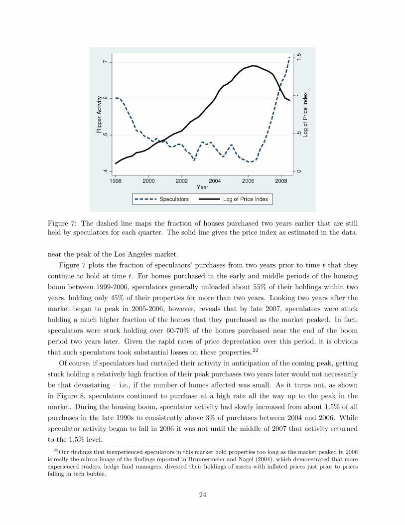
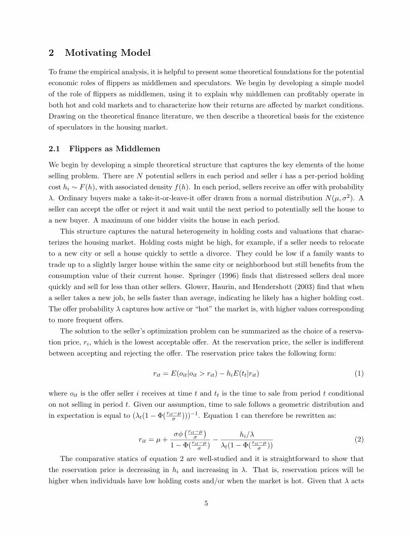
Figure 7: The dashed line maps the fraction of houses purchased two years earlier that are stillheld by speculators for each quarter. The solid line gives the price index as estimated in the data.

near the peak of the Los Angeles market.Figure 7 plots the fraction of speculators’ purchases from two years prior to time t that they

continue to hold at time t. For homes purchased in the early and middle periods of the housingboom between 1999-2006, speculators generally unloaded about 55% of their holdings within twoyears, holding only 45% of their properties for more than two years. Looking two years after themarket began to peak in 2005-2006, however, reveals that by late 2007, speculators were stuckholding a much higher fraction of the homes that they purchased as the market peaked. In fact,speculators were stuck holding over 60-70% of the homes purchased near the end of the boomperiod two years later. Given the rapid rates of price depreciation over this period, it is obviousthat such speculators took substantial losses on these properties.22

Of course, if speculators had curtailed their activity in anticipation of the coming peak, gettingstuck holding a relatively high fraction of their peak purchases two years later would not necessarilybe that devastating – i.e., if the number of homes affected was small. As it turns out, as shownin Figure 8, speculators continued to purchase at a high rate all the way up to the peak in themarket. During the housing boom, speculator activity had slowly increased from about 1.5% of allpurchases in the late 1990s to consistently above 3% of purchases between 2004 and 2006. Whilespeculator activity began to fall in 2006 it was not until the middle of 2007 that activity returnedto the 1.5% level.

22Our findings that inexperienced speculators in this market hold properties too long as the market peaked in 2006is really the mirror image of the findings reported in Brunnermeier and Nagel (2004), which demonstrated that moreexperienced traders, hedge fund managers, divested their holdings of assets with inflated prices just prior to pricesfalling in tech bubble.

24

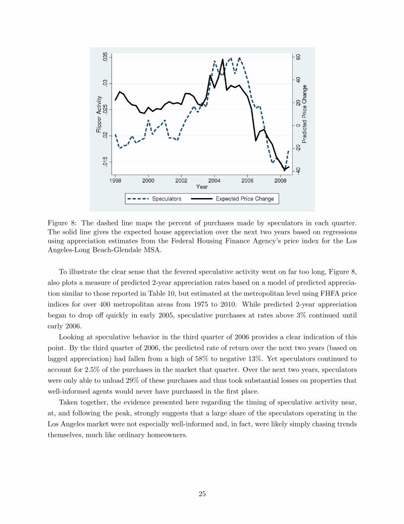
Figure 8: The dashed line maps the percent of purchases made by speculators in each quarter.The solid line gives the expected house appreciation over the next two years based on regressionsusing appreciation estimates from the Federal Housing Finance Agency’s price index for the LosAngeles-Long Beach-Glendale MSA.

To illustrate the clear sense that the fevered speculative activity went on far too long, Figure 8,also plots a measure of predicted 2-year appreciation rates based on a model of predicted apprecia-tion similar to those reported in Table 10, but estimated at the metropolitan level using FHFA priceindices for over 400 metropolitan areas from 1975 to 2010. While predicted 2-year appreciationbegan to drop off quickly in early 2005, speculative purchases at rates above 3% continued untilearly 2006.

Looking at speculative behavior in the third quarter of 2006 provides a clear indication of thispoint. By the third quarter of 2006, the predicted rate of return over the next two years (based onlagged appreciation) had fallen from a high of 58% to negative 13%. Yet speculators continued toaccount for 2.5% of the purchases in the market that quarter. Over the next two years, speculatorswere only able to unload 29% of these purchases and thus took substantial losses on properties thatwell-informed agents would never have purchased in the first place.

Taken together, the evidence presented here regarding the timing of speculative activity near,at, and following the peak, strongly suggests that a large share of the speculators operating in theLos Angeles market were not especially well-informed and, in fact, were likely simply chasing trendsthemselves, much like ordinary homeowners.

25

8 Conclusion

Making use of a large transactions database and a novel research design, this paper provides thefirst comprehensive study of intermediaries (middlemen and speculators) in the housing market:identifying (i) their activity, (ii) the sources of their returns, and (iii) the extent to which theiractivity is associated with local price dynamics. Our analysis for Los Angeles establishes thatmiddlemen and speculators follow distinct strategies for when and where to buy and generatereturns from almost completely distinct sources. Middlemen hold properties for very short periodsof time and earn most of their return by buying houses relatively cheaply; they operate throughoutbooms and busts in the market and target all types of neighborhoods. By contrast, speculatorsearn almost their entire return through timing the market, operate only during boom times, andtarget neighborhoods with the highest expected price appreciation. Entry by speculative flippersis strongly associated with the short-term amplification of neighborhood housing price bubbles.And, given their inexperience flipping homes and apparent difficulty anticipating and reacting tothe peak of the most recent housing boom, it seems likely that many of the speculators identifiedin the data are noise traders themselves rather than the rational arbitrageurs of modern financetheory.

This paper makes several important contributions to the literatures on housing and financialmarkets. Most directly, it expands our understanding of the microstructure of the housing market:establishing a number of new empirical facts about the activity of middlemen and speculators inthe market that generally conform to the roles prescribed in economic theory. More generally,our ability to identify speculators in the data and analyze their strategies and impact on themarket is relatively rare in the wider empirical finance literature. While not completely conclusive,our findings that speculators engage in positive feedback trading and may not be especially wellinformed about market fundamentals are strongly suggestive that speculators in this market havesubstantial destabilizing effects on prices, leading to an amplification of local housing price cycles.While this increased volatility has important economic consequences, any policy remedies need alsoaccount for the welfare-enhancing role that flippers play by providing liquidity as middlemen andin improving the physical stock of housing in older neighborhoods.

26

References

Abreu, D., and M. Brunnermeier (2002): “Synchronization Risk and Delayed Arbitrage,”Journal of Financial Economics, 66, 341–360.

(2003): “Bubbles and Crashes,” Econometrica, 71, 173–204.

Anenberg, E. (2010): “Loss Aversion, Equity Constraints and Seller Behavior in the Real EstateMarket,” Regional Science and Urban Economics, 41(1), 67–76.

Barberis, N., and R. Thaler (2003): A Survey of Behavioral Finance vol. 1 of Handbook ofEconomics and Finance, chap. 18. Elsevier.

Brunnermeier, M., and S. Nagel (2004): “Hedge Funds and the Technology Bubble,” Journalof Finance, 59(5), 2013–2040.

Case, K., J. Quigley, and R. Shiller (2003): “Home-buyers, Housing and the Macroeconomy,”BPHUP working paper # W04-004.

Case, K., and R. Shiller (1987): “On the Equilibrium Properties of Locational Sorting Models,”New England Economic Review, (September/October), 45–56.

(1989): “The Efficiency of the Market for Single-Family Homes,” American EconomicReview, 79(1), 125–137.

De Long, B., A. Shleifer, L. Summers, and R. Waldmann (1990a): “Noise Trader Risk inFinancial Markets,” Journal of Political Economy, 98, 703–738.

(1990b): “Positive Feedback Investment Strategies and Destabilizing Rational Specula-tion,” Journal of Finance, 45(2), 379–395.

Eichengreen, B., J. Tobin, and C. Wyplosz (1995): “Two Cases for Sand in the Wheels ofInternational Finance,” Economic Journal, 105, 162–172.

Fama, E. (1955): “The Behavior of Stock-Market Prices,” Journal of Business, 38, 34–105.

Friedman, M. (1953): Essays in Positive Economics. University of Chicago Press.

Genesove, D., and C. Mayer (2001): “Loss Aversion and Seller Behavior: Evidence from theHousing Market,” Quarterly Journal of Economics, 116(4), 1233–1260.

Glower, M., D. Haurin, and P. Hendershott (2003): “Selling Time and Selling Price: TheImpact of Seller Motivation,” Real Estate Economics, 26(4), 719–740.

Greenwood, R., and S. Nagel (2009): “Inexperienced Investors and Bubbles,” Journal ofFinancial Economics, 93, 239–258.

27

Haruvy, E., Y. Lahav, and C. Noussair (2007): “Traders’ Expectations in Asset Markets:Experimental Evidence,” American Economic Review, 97, 1901–1920.

Hendershott, T., and J. Zhang (2006): “A Model of Direct and Intermediated Sales,” Journalof Economics and Management Strategy, 15(2), 279–316.

Himmelberg, C., C. Mayer, and T. Sinai (2005): “Assessing High House Prices: Bubbles,Fundamentals, and Misperceptions,” Journal of Economic Perspectives, 19(4), 67–92.

Rust, J., and G. Hall (2003): “Middlemen versus Market Makers: A Theory of CompetitiveExchange,” Journal of Political Economy, 111(2), 353–403.

Shiller, R. (2003): “From Efficient Markets Theory to Behavioral Finance,” Journal of EconomicPerspectives, 17(1), 83–104.

Shleifer, A., and L. Summers (1990): “The Noise Trader Approach to Finance,” Journal ofEconomic Perspectives, 4(2), 19–33.

Smith, V., G. Suchanek, and A. Williams (1988): “Bubbles, Crashes and Endogenous Expec-tations in Experimental Spot Markets,” Econometrica, 56, 1119–1151.

Springer, T. (1996): “Single-Family Housing Transactions: Seller Motivations, Price, and Mar-keting Time,” Journal of Real Estate Finance and Economics, 13(3), 237–254.

Spulber, D. (1996): “Market Making by Price-Setting Firms,” Review of Economic Statistics,63(4), 559–580.

Summers, L., and V. Summers (1988): “When Financial Markets Work too Well: A CautiousCase for a Securities Transactions Tax,” Journal of Financial Services Research, 3(2-3), 163–188.

Tobin, J. (1974): The Eliot Janeway Lectures on Historical Economics in Honor of Joseph Schum-peter chap. The New Economics One Decade Older. Princeton University Press.

(1978): “A Proposal for International Monetary Reform,” Eastern Economic Journal, 4,153–159.

Vissing-Jorgensen (2003): NBER Macroeconomics Annual chap. Perspectives on BehavioralFinance: Does Irrationality Disappear with Wealth? Evidence from Expectations and Actions,pp. 139–193. MIT Press.

Wurgler, J., and E. Zhuravskaya (2002): “Does Arbitrage Flatten Demand Curves forStocks?,” Journal of Business, 75, 583–608.

28