speech attribute detection using deep learningcs.uef.fi/sipu/pub/speechatrib-kukanov.pdf · in this...

Speech Attribute Detection Using Deep Learning

Ivan Kukanov

Master’s Thesis

Faculty of Science and Forestry

School of Computer Science

August 2015

UNIVERSITY OF EASTERN FINLAND, Faculty of Science and Forestry, JoensuuSchool of ComputingSchool of Computer Science

Student, Ivan Kukanov : Speech Attribute Detection Using Deep LearningMaster’s Thesis , 82 p., 3 appendix (11 p.)Supervisors of the Master’s Thesis : Dr. Ville HautamäkiAugust 2015

Abstract:

In this work we present alternative models for attribute speech feature extraction basedon the two state-of-the-art deep neural networks: convolutional neural networks (CNN) andfeed-forward neural network with pretraining using stack of restricted Boltzmann machines(DBN-DNN). These attribute detectors are trained using data-driven approach across all lan-guages in the OGI-TS multi-language telephone speech corpus. Thus, such a detectors canbe considered as the universal phonetician alphabet (UPA), which can detect phonologicallydistinctive articulatory features belonging to all languages. Moreover, articulatory featurescan capture foreign accents characteristics and further these models will be utilized to solvethe foreign accent recognition problem.

We consider two types of articulatory feature detectors, these are manner and place ofarticulation, which extract characteristics of the human speech production process from thespeech dataset. Evaluating on the OGI-TS dataset, the results in terms of Average EqualError Rate and Detection Error Tradeoff show that the attribute model based on the CNNconsistently outperform the DBN-DNN model. Attribute detectors with CNN, versus DBN-DNN model, reduce the AvgEER producing 18.8% relative improvements for manner ofarticulation and producing 10.3% relative improvements for place of articulation. Also, man-ner speech features are detected more accurately then place features 11.46% versus 14.06%AvgEER.

Keywords:

deep neural networks, restricted Boltzmann machine, convolutional neural network, data-driven speech attributes, manner of articulation, place of articulation, foreign accent recog-nition

ii

Foreword

Firstly, I would like to express my sincere gratitude to my supervisor Dr. Ville Hautamäki for

the continuous support of my Master’s degree study and related research, for his patience,

motivation, and kindness, for giving me the opportunity to work at the Speech and Image

Processing Unit. I was never bored a minute while working on several research projects

over the course time. I also want to thank my reviewer Dr. Cemal Hanilci for his insightful

comments and encouragement, and kindly proof-reading my thesis.

I am grateful to the whole staff of the School of Computing for help and assistance, for

providing me with all the necessary facilities to implement my research projects. Special

thanks to Juha Hakkarainen for his prompt response in my technical questions and requests;

thanks for rebooting the GPU server while it got stuck with calculations at any time of the

day or night, weekends or vacations. I thank members of our research group and colleagues,

special thanks to Alexandr Sizov and Anna Fedorova for nice time spent in and out of the

lab. Also thanks to my group mates of the International Master’s Degree Programme in

Informational Technology.

Finally, I want to thank the most valuable persons in my life, my parents Nikolay and

Tatiana, and my brother Nikolay for their love and unfailing support during rough times, who

encouraged me to spend time and effort on this thesis.

Joensuu September 4, 2015 Ivan Kukanov

iii

List of Abbreviations

ASR Automatic Speech Recognition

CNN Convolutional Neural Networks

DBN-DNN Deep Belief Neural Networks

DNN Deep Neural Networks

iv

Contents

1 Introduction 11.1 Goals . . . . . . . . . . . . . . . . . . . . . . . . . . . . . . . . . . . . . . 3

2 Artificial Neural Networks 52.1 Single-layer Perceptron . . . . . . . . . . . . . . . . . . . . . . . . . . . . . 5

2.2 Multi-layer Neural Networks . . . . . . . . . . . . . . . . . . . . . . . . . . 9

2.3 Training approaches . . . . . . . . . . . . . . . . . . . . . . . . . . . . . . . 11

3 Restricted Boltzmann Machine 173.1 Notes from statistical physics . . . . . . . . . . . . . . . . . . . . . . . . . . 18

3.2 Restricted Boltzmann Machine inference . . . . . . . . . . . . . . . . . . . . 19

3.2.1 Free energy function . . . . . . . . . . . . . . . . . . . . . . . . . . 22

3.3 Contrastive Divergence . . . . . . . . . . . . . . . . . . . . . . . . . . . . . 24

4 Convolutional Neural Networks 314.1 Properties . . . . . . . . . . . . . . . . . . . . . . . . . . . . . . . . . . . . 32

4.2 Network architecture . . . . . . . . . . . . . . . . . . . . . . . . . . . . . . 34

5 Deep Neural Network Pre-training 395.1 Motivation for deepness . . . . . . . . . . . . . . . . . . . . . . . . . . . . . 39

5.2 Deep Belief Network pre-training . . . . . . . . . . . . . . . . . . . . . . . 40

5.3 Fine-tunning . . . . . . . . . . . . . . . . . . . . . . . . . . . . . . . . . . . 44

6 Application Neural Networks for Attribute Detection 476.1 System Overview . . . . . . . . . . . . . . . . . . . . . . . . . . . . . . . . 47

6.2 Speech Feature Extraction . . . . . . . . . . . . . . . . . . . . . . . . . . . 50

6.3 System Settings . . . . . . . . . . . . . . . . . . . . . . . . . . . . . . . . . 51

6.3.1 DBN-DNN topology . . . . . . . . . . . . . . . . . . . . . . . . . . 51

6.3.2 Convolutional Neural Networks topology . . . . . . . . . . . . . . . 52

v

7 Experiments and Results 557.1 Dataset . . . . . . . . . . . . . . . . . . . . . . . . . . . . . . . . . . . . . 55

7.2 Performance measure . . . . . . . . . . . . . . . . . . . . . . . . . . . . . . 57

7.2.1 DET curves . . . . . . . . . . . . . . . . . . . . . . . . . . . . . . . 58

7.2.2 Average Equal Error Rate . . . . . . . . . . . . . . . . . . . . . . . 58

7.2.3 Visualization of trained weights . . . . . . . . . . . . . . . . . . . . 62

8 Conclusions 65

A Manner Multi Labels mapping to Phonemes 77

B Place Multi Labels mapping to Phonemes 81

C Equal Error Rate for all detectors and different Neural Network topologies 85

vi

CHAPTER 1

Introduction

This thesis deals with a foreign accent recognition in general and more specifically it is

devoted to particular speech features which characterize different language accents. In au-

tomatic foreign accent recognition the mother tongue (L1) of non-native speakers has to be

recognized given a spoken segment in a second language (L2) [31]. This task is taking much

attention in the speech community because accent usually negatively affects the performance

of conventional automatic speech recognition (ASR) systems [5]. The problem of the exist-

ing ASR systems that these are working mostly with the native speech only, and the accuracy

dramatically reduces when words are uttered with an alternative pronunciation (e.g. foreign

accent)[29]. Foreign accents also negatively affect other speech systems such as automatic

speaker and language recognition [5, 4]. Moreover, foreign accent recognition plays a vital

needs for border control security systems [83]. It may help officials to detect immigrants

with a fake passport by recognizing actual country and region of spoken foreign accent.

The main idea why the foreign accents may be recognized is because of the deviation

from the standard pronunciation and influences of language L1 on L2 [66, 85]. That is

non-native speakers often tend to alter some phoneme features when pronouncing a word

in L2 because they usually only partially manage its pronunciation. For example, Italians

often aspirate the /h/ sound in words such as house, hill or hotel[85]. Another anomaly

in pronunciation may be replacing an unfamiliar phoneme in L2 with the one that closer

and easier to utter in L1[85]. As an example from [85], word closely in English can be

pronounced as «k l ow s l iy», in Japanese it may has the next phonetician content «k uh l ow

s l iy».

A naive solution for accent recognition could be the use of language recognition tech-

1

CHAPTER 1. INTRODUCTION

niques based on n-gram phoneme statistics, but this approach can not be directly used, be-

cause the collected phoneme statistic would match the L2 language. The problem here is that

every language has its own phone set. The solution is to create universal phonetic alphabet

(UPA) [80]. In previous works [80, 79, 57, 77, 56] it was proposed to use speech articulatory

features as the UPA.

Speech articulatory features such as manner (fricative, glide, nasal, silence, stop, voiced,

vowel) and place (coronal, dental, glottal, high, labial, low, mid, palatal, silence, and ve-lar) can capture language and accent variations. Experimental evidence showed their effec-

tiveness in foreign accent recognition [32, 9].

Using universal articulatory features we can analyse the statistical model for pair L1-

L2 languages. For instance, if we take English and Japanese pronunciation of word closely

and represent it in manner attribute transcription (using mapping tables from Appendix A),

for English it will be «stop gs_voiced voiced_vowel fric gs_voiced voiced_vowel» and for

Japanese «stop voiced_vowel gs_voiced voiced_vowel fric gs_voiced voiced_vowel». These

two transcriptions differ in one manner attribute («voiced_vowel»). Thus, gathering such a

statistic about different attribute content of the pronunciations we may recognize the foreign

accents or dialects.

In [8] it was proposed successful bottom-up implementation of the foreign accent recog-

nition model based on front-end attribute detectors. The low-level detectors were modeled

using artificial neural networks (ANN) with single-hidden non-linear layer and soft-max out-

put layer. However, the baseline speech attribute front-end showed large error rate variance

[80]. It was needed more advanced approach to improve the detectors’ accuracy.

Further, we discuss why the deep learning approaches have been chosen. The biggest ad-

vance occurred nearly four decades ago with the introduction of the expectation-maximization

(EM) algorithm for training Hidden Markov Models (HMMs), see historical review on HMM

[6, 28]. With the EM algorithm, it became possible to develop speech systems using the rich-

ness of Gaussian mixture models (GMMs) [58] to represent the relationship between HMM

states and the acoustic input. Despite their advantages, GMMs have a serious shortcoming

[40]. Artificial neural networks trained by backpropagating have the potential to learn much

better models. In fact two decades ago, it was achieved some success using ANN with a

single layer of non-linear hidden units. However, there was no adequate learning algorithm

for training neural networks with many hidden layers on large amount of data. Also the

computer hardware performance were not sufficient to seriously challenge GMMs [40].

2


Over the last decade, advances in both machine learning and graphics processing unit

(GPU) computation led to more efficient methods. In 2006 Geoffrey Hinton’s paper work

[40] made a significant impact in neural networks and turned researchers mind to this field.

Since that time, it became possible to train networks with many layers of non-linear units and

a very large output layers. The new study of deep learning has appeared which is a branch of

machine learning based on a set of algorithms that model high-level abstractions in data by

using model architectures composed of multiple non-linear transformations [25].

New deep learning algorithms led to significant advances in different areas. In some

fields these even outperform human abilities: in [88] it is proposed deep learning approach

which beats humans in IQ test, in [34, 47] Microsoft and Google have beat the human bench-

mark at image recognition of 5.1% errors. Deep neural networks (DNNs) have been success-

fully applied in across a range of speech processing tasks as well, such as conversational-style

speech recognition [76], noise robust applications [91], multi- and cross-lingual learning

techniques [62] and others. Inspired by the success of those applications, we want to explore

the use of DNNs to extract manner and place of articulation attributes to be used in automatic

accent recognition systems.

1.1 Goals

The main goal of the research is to improve the existing foreign accent recognition system

[32]. In order to refine the whole system we have to improve components it consists of. In

this thesis we will improve the front-end speech articulatory detectors. For that problem the

next tasks will be solved:

• implement a model for detecting speech attributes of articulation using deep learning

approaches;

• the proposed model have to satisfy the attribute paradigm [56];

• investigate performance of the proposed model and apply to the foreign accent recog-

nition.

3


4

CHAPTER 2

Artificial Neural Networks

In this chapter we briefly consider simple neural perceptron. After that we move to the

multilayer neural networks, review its training algorithm Backpropagation and its advantages

and drawbacks.

2.1 Single-layer Perceptron

People and animals from day to day use their brain, eyes, ears to make decisions and train

itself. When we socialize with each other we do not even think of processes of recognition

in the brain we easily and automatically recognize the words of people with different voices.

For human brain it is easy to recognize any objects, sounds, printed or handwritten text, we

do it on the fly and subconsciously.

On the other hand, scientists studied the issues of the brain activity modeling and how it

solves such a complex tasks. Firstly natural nervous system was mentioned in primitive un-

derstanding by René Descartes in XVII century [30]. In his work, Descartes firstly proposed

the existence of human reaction on the external events, it was the first steps of the founding

of reflex theory.

In the modern understanding nervous system was described in works of Camillo Golgi

and Santiago Ramon y Cajal. They got the Nobel Prize in Physiology or Medicine in 1906

«in recognition of their work on the structure of the nervous system» [1]. These study made

the ground theory of the natural neural networks and moder biology.

5

CHAPTER 2. ARTIFICIAL NEURAL NETWORKS

Later on these understandings of biological neural networks mathematical artificial neu-

ral network (ANN) approach emerged. Artificial neural networks are mathematical models

which have extremely simplified analogues of natural neural networks. But even using just a

basic principals of biological neural systems it is enough to successfully solve some practical

problems.

McCulloch-Pitts Neural Network Model. Let given X is a general space of objects and

Y is a space of responses, there is relation y∗ : X → Y which we know only on training

subset of objects X l = (xi, yi)li=1, yi = y∗ (xi). We need to develop algorithm a : X → Y

which will approximate objective function y∗ on the whole space of objects X . This is a

basic problem of machine learning. Further, let consider that objects can be described by n

features fj : X → R, j = 1, n, or in vector form (f1 (x) , . . . , fn (x))T ∈ Rn.

First neural network was proposed by Warren McCulloch and Walter Pitts in 1943 [61].

It was simple linear perceptron, see Figure 2.1.

Figure 2.1: Perceptron model of Warren McCulloch and Walter Pitts and biological neuralcell [90].

This model get n-dimensional feature vector as the input

x =(x1, . . . , xn

)T ≡ (f1 (x) , . . . , fn (x))T ,

here object x identified with its feature vector. For simplicity features are supposed to be

binary. These features are multiplied on the respective weights w = (w0, . . . , wn)T . The

neuron’s output is 0 or 1, it is determined by the weighted input sum. If sumn∑j=1

wjxj is

greater then threshold w0 then neuron is activated and output 1, otherwise 0. In mathematical

terms it means the output from the neural network is a(x):

6


a (x) = σ

(n∑j=1

wjxj − w0

), (2.1)

where σ (z) is an activation function. In perceptron model activation function is a simple

Heaviside step function:

σ (z) = θ (z) = [z > 0] =

0, z < 0,

1, z > 0(2.2)

McCulloch-Pitts model is equivalent to the linear step classifier. Later perceptron model

was extended to the neural networks with real value inputs and outputs and with different

activation functions.

Activation functions. There are different types of neural activation functions, the choice

of them depends on the practical task. Commonly used activation functions are shown on the

Figure 2.2. Sometimes neurons are called regarding its activation function.

Figure 2.2: Linear, logistic and hyperbolic tangent functions and their derivatives.

Binary threshold neurons [93] which is described above, it is another name for McCulloch-

Pitts model. Linear neurons [93] is the simplest kind of neurons. It has linear activation

function

σlinear(z) = z. (2.3)

Hence, we have connection of neural networks with the linear regression model

7


a (x) =n∑j=1

wjxj − w0 = wTx. (2.4)

It is computationally limited because the superposition of such neurons in many layers still

gives linear model. Sigmoid neurons produces real valued outputs that is bounded between 0

and 1. This kind of neurons is very frequently used in neural nets

σlogistic (z) =1

1 + e−z. (2.5)

Hyperbolic tangent function [93] is a neuron with activation function

σtanh (z) = tanh (z) =ez − e−z

ez + e−z. (2.6)

Linear (2.3), sigmoid (2.5) and hyperbolic tangent (2.6) activation functions are smooth and

differentiable (see Figure 2.2). Moreover, these derivatives are either constant or defined in

terms of the original function

σ′linear (z) = 1

σ′logistic (z) = σlogistic (z) (1− σlogistic (z))

σ′tanh (z) = 1− σ2tanh (z)

(2.7)

It is a key feature that makes training very efficient and convenient for implementation

of the Back-propagation approach (see later in the Section 2.3).

Rectified linear neurons (ReLU) [93] combines the ideas of both previous binary thresh-

old and linear neurons. Firstly, it computes weighted sum of its inputs, as usually, and then

it produces output of non-linear activation function

σ (z) =

z, if z > 0,

0, otherwise.(2.8)

So, above zero it is linear and at zero it makes a «hard» decision.

8


2.2 Multi-layer Neural Networks

Computer scientists went further and again inspired by the human brain. Similarly the natural

neurons works together and have difficult multilayer structure, mathematicians brought this

idea to the artificial multilayer neural networks.

Figure 2.3: Multi-layer neural network with one hidden layer [87].

On the Figure 2.3 it is represented multilayer network with one hidden layer for simplic-

ity. On the input layer we send n-dim feature vector, then these features simultaneously goes

to the H neurons of the first hidden layer. On the hidden layer we acquire weighted sum of

the features which goes through the activation function. After that it moves to next layer and

so on.

On the output we get signals am. In general case neural networks can have arbitrary num-

ber of neurons in hidden layers and hidden layers itself. Number of output signals usually

corresponds to number of classes in classification problem.

Properties of multilayer networks. The main question for machine learning is what kind

of function neural networks can approximate? Here we list some features on neural networks

which answer this question [33].

• Any boolean function (disjunctive normal form) can be represented by 2-layers artifi-

cial neural network in {0, 1}n space. It means if input features are binary and we are

solving binary classification problem then it is enough to have 2-layers to approximate

9


any boolean function [33].

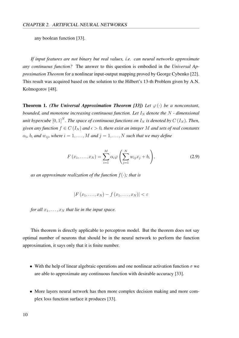
If input features are not binary but real values, i.e. can neural networks approximate

any continuous function? The answer to this question is embodied in the Universal Ap-

proximation Theorem for a nonlinear input-output mapping proved by George Cybenko [22].

This result was acquired based on the solution to the Hilbert’s 13-th Problem given by A.N.

Kolmogorov [48].

Theorem 1. (The Universal Approximation Theorem [33]) Let ϕ (·) be a nonconstant,

bounded, and monotone increasing continuous function. Let IN denote the N - dimensional

unit hypercube [0, 1]N . The space of continuous functions on IN is denoted by C (IN). Then,

given any function f ∈ C (IN) and ε > 0, there exist an integer M and sets of real constants

αi, bi and wij , where i = 1, . . . ,M and j = 1, . . . , N such that we may define

F (x1, . . . , xN) =M∑i=1

αiϕ

(N∑j=1

wijxj + bi

), (2.9)

as an approximate realization of the function f(·); that is

|F (x1, . . . , xN)− f (x1, . . . , xN)| < ε

for all x1, . . . , xN that lie in the input space.

This theorem is directly applicable to perceptron model. But the theorem does not say

optimal number of neurons that should be in the neural network to perform the function

approximation, it says only that it is finite number.

• With the help of linear algebraic operations and one nonlinear activation function σ we

are able to approximate any continuous function with desirable accuracy [33].

• More layers neural network has then more complex decision making and more com-

plex loss function surface it produces [33].

10


2.3 Training approaches

In 1949 the neuropsychologist Donald O. Hebb developed the theory of the relationship of

the brain and cognitive processes [35]. In his works he described some ideas of artificial

neural network structuring and layers composition. Hebb proposed hypothetical ideas of

neural networks training which made up the ground theory of all nowadays neural network

algorithms, commonly known as «Hebb’s postulate» [33]. These are the next:

1. if two neurons from different sides of synapse are activated simultaneously, then synapse

«weight» is increasing;

2. if two neurons from different sides of synapse are activated asynchronously, then

synapse «weight» is decreasing or synapse is removed.

In 1958 Frank Rosenblatt, inspired by the works of McCulloch, Pitts and Hebb, devel-

oped Rosenblatt’s Perceptron [70]. It was shown that perceptron can perform basic logical

operations (conjunction and disjunction) and has the convergent learning algorithm (per-

ceptron convergence theorem [33]). The Rosenblatt’s Perceptron power is limited it can be

applied only for linearly separable classes [33].

After Marvin Minski critical book about the perceptoron model [63] the interest to the

neural networks was dramatically reduced. He analyzed mathematical inconsistency and

limitations of the perceptron model (XOR function problem, see Figure 2.4).

The interest to the neural networks was refreshed after developing the Error Backpropa-

gation algorithm by D.E. Rumelhart, G.E. Hinton and R. J. Williams in 1986 [71].

Error Backpropagation. Consider Figure 2.3, we are given X = Rn features and Y =

RM corresponding vector of responses. In our simple case one-hidden layer of neural net-

work has [H(n+ 1) + (H + 1)M ] unknown parameters (vector of all weights w) which we

have to fit using training set. Usually the complexity of problem increases proportionally

with the number of unknown parameters (when we add new layers). But in neural networks

we can avoid this issue using efficient gradient method error backpropagation.

Let output layer contains M neurons with activation functions σm and outputs am, m =

11


Figure 2.4: Limitations of the Rosenblatt’s Perceptron, XOR function problem.

1, . . . ,M signals; hidden layer has H neurons with activation functions σh and outputs uh,

h = 1, . . . , H signals. Weights between the neurons from the hidden layer and the output

layer are denoted as whm. Weights between the input layer neurons and the hidden layer are

denoted as wjh.

The output signals am after the features xi (i-th object features from the training set) pass

through the all layers are calculated as superposition of output signals on intermediate layers:

am = σm

(H∑h=0

whmuh (xi)

); uh (xi) = σh

(n∑j=0

wjhxji

), (2.10)

where xji is the j-th component of the i-th object feature vector.

The problem of weights training is the next we have to minimize the value of the loss

function on the training set (xi, yi) of size l:

Q (w) =l∑

i=1

L (w, xi, yi)→ minw. (2.11)

Popular distance measures can be used for the loss function. For the regression task [93], the

mean square error (MSE) criterion is typically used,

LMSE (w, xi, yi) =1

2‖xi − yi‖2 . (2.12)

12


For the classification task, where yi is a response (probability distribution) on the i-th object

and the cross-entropy (CE) criterion

LCE (w, xi, yi) = −M∑m=1

ymi log [νm (xi)], (2.13)

where ymi = Pemp (m|xi) is the empirical (observed in the training set) probability that the

object xi belongs to class m, and νm (xi) is the same probability estimated from the DNN

νm (xi) = PDNN (m|xi) = softmaxm (zmi ) =exp (zmi )M∑m=1

exp (zmi )

, (2.14)

and zmi =H∑h=0

whmuh (xi) - m-th weighted signal on the final layer. For more details of

softmax layer and cross-entropy criteria usage see [93], [67].

In our example for simplicity we will utilize MSE criterion. In order to minimize our cost

function (2.11) we could use stochastic gradient descend to search the minimum [27] as for

single percetron training. But it is difficult to calculate gradient directly using the loss func-

tion L (w, xi, yi), the complexity of such problem is in the order of O([Hn+HM ]2

). With

the aid of error backpropagation we can reduce the complexity to order ofO (3[Hn+HM ]).

The point of the error backpropagation is in the efficient differentiation of superposition of

functions (chain rule differentiation). We effectively store intermediate results of the algo-

rithm in the units of the neural network and then quickly calculate the total gradient.

Further for our one-hidden layer example the loss function Li(w) = LMSE (w, xi, yi)

proposed to be the mean square error calculated on every object xi output signal, after for-

ward pass:

Li (w) =1

2

M∑m=1

(am (xi)− ymi )2. (2.15)

So, we have to derive partial derivatives of the loss function Li with respect to the output

signals am of the final layer:

∂Li (w)∂am

= am (xi)− ymi = εmi (2.16)

13


here we denote the partial derivative as εmi , i.e. error estimation on the sample object xi with

response yi.

Now consider derivatives of the hidden layer h with respect to their outputs:

∂Li (w)∂uh

=M∑m=1

(am (xi)− ymi )σ′mwhm =M∑m=1

εmi σ′mwhm = εhi , (2.17)

this derivative we also call as «error estimation» εhi of network on the hidden layer, σ′m =

σ′m

(H∑h=0

whmuh (xi)

)is the derivative of the activation function calculated on the same ar-

gument as in (2.10). If sigmoid activation function is used then the derivative could be

effectively calculated as σ′m = σm (1− σm).

We can notice that εhi is calculated using εmi if we run the neural network backward and

set εmi σ′m on the output units and get εhi on the input units as shown on Figure 2.5. That is

why it is called backpropagation.

Figure 2.5: Error backward running.

When we have derivatives (2.16) and (2.17) with respect to am and uh we can easily infer

gradient of loss function Li (w) with respect to weights:

∂Li (w)∂whm

=∂Li (w)∂am

∂am

∂whm= εmi σ

′mu

h, h = 0, . . . , H, m = 1, . . . ,M ; (2.18)

∂Li (w)∂wjh

=∂Li (w)∂uh

∂uh

∂wjh= εhi σ

′hxj, j = 0, . . . , n, h = 1, . . . , H. (2.19)

If we have more layers then derivatives are inferred using same chain rule. Algorithm for

14


any number of hidden layers is derived in [93].

Therefore, we have all needed information to summarize the error backpropagation for

two-layer neural network in Algorithm 1.

Algorithm 1 two-layer neural network training using Error Backpropagation

Input: X l = (xi, yi)li=1 - training set, xi ∈ Rn, yi ∈ RM ;

H - number of units in hidden layers;η - learning rate;Q - loss function, initial value is calculated using equation (2.11);λ - constant parameter from interval [0; 1];

Output: weights wjh, whm;

1: Initialisation: with small random numberswjh := random

(− 1

2n, 12n

);

whm := random(− 1

2H, 12H

);

2: repeat3: randomly choose xi;4: forward pass:

uhi := σh

(J∑j=0

wjhxi

);

ami := σm

(H∑h=0

whmuh (xi)

);

εmi := ami − ymi ;

Li :=M∑m=1

(εmi )2;

5: backward pass:

εhi :=M∑m=1

εmi σ′mwhm, for all h = 1, . . . , H;

6: gradient step:whm := whm − ηεmi σ′mum, for all h = 0, . . . , H , m = 1, . . . ,M ;wjh := wjh − ηεhi σ′hxj , for all j = 0, . . . , n, h = 1, . . . , H;

7: Q := (1− λ)Q+ λLi;8: until Q stabilized;

Advantages of Error Backpropagation.

• Backpropagation is efficient algorithm, it can be easily parallelized [93].

• The algorithm is very flexible for training, i.e. it can be easily generalized on any

activation functions σ and loss functions L. Moreover, every neural unit can has its

own activation function. There are no restrictions on the number of input-output units

15


and hidden layers. Any method of optimization can be used for training (gradient

descent, conjugate gradient, the Newton–Raphson method).

Disadvantages of Error Backpropagation.

• Convergence is not guaranteed, because gradient descent tends to stuck in many local

minima of the loss function L [93]. In order to improve convergence a lot of tricks and

heuristics are used [52], [54].

• Excessive number of weight parameters w can lead to overfitting of the model [93].

• Vanishing gradient problem [44], [45]. If sigmoid or hyperbolic tangent activation

functions are used then vanishing gradient problem appears. It means the larger values

of weightsw on the input of the unit the smaller value of the derivation σ′ on the output.

Therefore, weight correction on the backward pass of the backpropagation algorithm

is very tiny for multi layer perceptron (more then 2 hidden layers).

16

CHAPTER 3

Restricted Boltzmann Machine

Vanishing gradient problem was shown in training artificial neural networks using gradient

based backpropagation approaches (see [45]). Despite the tempting power of the neural net-

works that these are able to approximate any continuous function, it takes a lot of time to train

them and there was no efficient algorithm but «tricky» backpropagation. With the advent of

the backpropagation algorithm in the 1986, many researchers tried to train supervised deep

artificial neural networks from scratch, initially with little success. Interest to neural net-

works dramatically decreased at that time and since 1992 - 2005 («period of oblivion») there

were no any outstanding results in this field.

Gradient vanishing problem forced scientists to reject backpropagation algorithm and in-

vent other approaches for training neural networks. In 2005 Geoffrey Hinton et al. suggested

unsupervised pre-training approach [40]. It means that firstly we cluster training objects,

learn generally useful feature detectors, and only after that we name that clusters, i.e. by

supervised backpropagation we classify the data.

The deep model of Geoffrey Hinton involves learning the distribution of a high level

representation using successive layers of binary or real-valued latent variables. It uses a

restricted Boltzmann machine [82] to model each new layer of higher level features.

17

CHAPTER 3. RESTRICTED BOLTZMANN MACHINE

3.1 Notes from statistical physics

Before we go deeper into the Boltzmann Machine it would be correctly to mention what is

the ground behind this techniques.

Further we remind Boltzmann distribution from statistical mechanics [49]. Let’s imagine

some mechanical system with many degrees of freedom, e.g. in statistical physics particles

of ideal gas are considered as such system. This system can be in one of the many states

with some probability pi of that state i. Some energy Ei of the whole mechanical system

corresponds to that state i.

Figure 3.1: Ensemble canonically distributed over energy, for a quantum system consistingof one particle in a potential well: dependency of number of states, temperature and energyof the system [89].

Then probability pi of the state i is defining as Boltzmann-Gibbs distribution in thermo-

dynamic equilibrium conditions between the mechanical system and environment which is

represented as

pi =1

Zexp

(− EikB · T

)and (3.1)∑

i

pi = 1, (3.2)

where T is absolute temperature, kB is the Boltzmann constant, Ei is some energy of the

whole mechanical system, Z is the partition (normalization) function

18


Z =∑i

exp

(− EikB · T

). (3.3)

Boltzmann probability distribution (3.1) is an exponential distribution which is derived from

the Gibbs canonical distribution and canonical ensemble, for more details see statistical

mechanics [84], [49], [20].

The main theoretical facts from statistical physics about energy function [49] which

are playing the basis role in the Energy-Base learning [55], [53], [68] and will be used in

Restricted Boltzmann Machine:

1. state with low energy has more chances to appear than state with high energy;

2. when the temperature is decreasing states will appear more frequently from the small

subset of states with low energy, see Figure 3.1. That is when the temperature T

is high then particles move «more chaotically», the system has more states and can

easily move from state to state. When the temperature T is reduced number of system

states is decreasing. In ideal case system will have just one state when the temperature

T = 0.

3.2 Restricted Boltzmann Machine inference

A Restricted Boltzmann machine (RBM) is a generative stochastic artificial neural network

that can learn a probability distribution over its set of inputs. RBM was originally invented

under the name Harmonium by Paul Smolensky in 1986 [81]. It became very popular only

after Geoffrey Hinton and collaborators developed training algorithm for RBM [18]. It found

applications in dimensionality reduction [41], classification [51], collaborative filtering [75],

feature learning [21] and topic modeling [74].

So far, in Section 2 we consider neural networks that could learn to predict from an input

a particular target or class labels, that we have seen with Feed-forward neural network. Now

we are going to consider unsupervised RBM training that would learn something about data

based on the training input vector x, this approach extracts meaningful features from the data.

However, it can be trained in supervised way as well. RBM also allows us a leverage of the

availability of the unlabeled data. When we have small amount of labeled training set and

we also have a lot of unlabeled samples. This is called a semi-supervised learning problem.

19


RBM is an undirected bipartite graphical model shown on Figure 3.2. It defines the

distribution over the input vector x (layer of visible units), it is going to model the distribution

of these training data using layer of hidden units h. Notice, for simplicity, that x and h are

binary random variables, such RBM is called Bernoulli-Bernoulli. There are also Gaussian-

Bernoulli (real valued x and binary h) and Gaussian-Gaussian (real valued x and real valued

h). Later we explain how to generalize to other types of units that might be a real value.

Figure 3.2: Restricted Boltzmann Machine topology.

In order to define the distribution of training set which involves the latent variables which

corresponds to hidden units h, let first define the Energy Function:

E (x, h) = −hTWx− cTx− bTh, (3.4)

where h ∈ {0, 1}Nh×1 is the vector of hidden units, x ∈ {0, 1}Nx×1 is the vector of visible

units, W ∈ RNh×Nx is the matrix of connection weights, c ∈ RNx×1 and b ∈ RNh×1 are the

bias vectors.

The probability of the state (x, h) with the Energy Function E(x, h) of the visible and

hidden units configuration is defined using Boltzmann-Gibbs distribution (3.1)

p (x, h) =exp (−E (x, h))

Z, (3.5)

where Z =∑x,h

e−E(x,h) is the normalization factor known as the partition function. Unfortu-

nately, partition function is intractable for RBM and later we are going to avoid its calculation

[93].

Let consider inference of the posterior probability of h given visible input x. The first

20


fact to know is that the full conditional distribution factorizes. It can be written as the product

of each individual hidden unit given vector of visible units:

p (h|x) =∏j

p (hj|x). (3.6)

We can easily prove this

p (h|x) = p (x, h)∑̃h

p(x, h̃) =

=exp

[hTWx+ cTx+ bTh

]∑h̃∈{0,1}Nh

exp[h̃TWx+ cTx+ bT h̃

] =

=

exp

[∑j

hjWj,∗x+ bjhj

]∑̃h1

· · ·∑̃hNh

exp

[∑j

h̃jWj,∗x+ bjh̃j

] =

=

∏j

exp [hjWj,∗x+ bjhj]∑̃h1

· · ·∑̃hNh

∏j

exp[h̃jWj,∗x+ bjh̃j

] =

=∏j

exp [hjWj,∗x+ bjhj]∑h̃j∈{0,1}

exp[h̃jWj,∗x+ bjh̃j

] =

=∏j

exp [hjWj,∗x+ bjhj]

1 + exp [bj +Wj,∗x]=∏j

p (hj|x).

whereWj,∗ denotes the j-th row of matrixW . It means that all the hidden units are condition-

ally independent given the values of the visible layer. It is obvious because of the topology

of the RBM, hidden units have no connections with each other.

Remind that we consider binary hidden and visible random vectors, i.e. Bernoulli-

Bernoulli RBM. Then we can derive probability when hidden unit is equal to one given

21


visible vector:

p (hj = 1|x) = 1

1 + exp [− (bj +Wj,∗x)]=

= σlogistic (bj +Wj,∗x) , (3.7)

where Wj,∗ denotes the j-th row of matrix W . For the binary visible neurons x given h we

have similar symmetrical form of posterior probability:

p (x|h) =∏k

p (xk|h), (3.8)

and similarly probability when visible unit is active

p (xk = 1|h) = 1

1 + exp [− (ck + hTW∗,k)]=

= σlogistic(ck + hTW∗,k

), (3.9)

where W∗,k means the k-th column of the matrix W . These previous results can be easily

derived.

Notice that inference for RBM hidden units (3.7) is just a sigmoid of the linear transfor-

mation and it is equal to computation of the feed-forward neural network with sigmoid unit

(2.1) no matter whether binary or real-valued inputs are used. This fact allows us to use the

weights of an RBM to initialize a feed-forward neural network with sigmoidal hidden units

[93].

3.2.1 Free energy function

Further the concept of free energy function will be considered. Let us infer the marginal

probability of the input vector x. We can write it down as sum of the probability of observing

the hidden layer with visible units through the all binary hidden vectors, i.e. we get marginal

probability distribution summing over all values of h

22


p (x) =∑

h∈{0,1}Nh

p (x, h) =∑h

exp [−E (x, h)]

Z=

=

exp

[cTx+

Nh∑j=1

log [1 + exp (bj +Wj,∗x)]

]Z

=

=exp (−F (x))

Z, (3.10)

where Wj,∗ denotes the j-th row of matrix W , F (x) is the free energy function

F (x) = − log

[∑h

e−E(x,h)

]. (3.11)

Equation (3.10) can be proved as:

p (x) =

∑h∈{0,1}Nh

exp[hTWx+ cTx+ bTh

]Z

=

=

exp[cTx]∑h1

· · ·∑hNh

exp

[∑j

hjWj,∗x+ bjhj

]Z

=

=

exp[cTx](∑

h1

exp [h1W1,∗x+ b1h1]

). . .

(∑hNh

exp [hNhWNh,∗x+ bNh

hNh]

)Z

=

=exp

[cTx](1 + exp [W1,∗x+ b1]) . . . (1 + exp [WNh,∗x+ bNh

])

Z=

=

exp

(cTx+

Nh∑j=1

log [1 + exp (Wj,∗x+ bj)]

)Z

=exp (−F (x))

Z. (3.12)

So, in order to maximize the probability of the input training x in (3.12) we need to find such

rows of weight matrix Wj,∗ and bias bj that will well align together with that x, i.e. represent

meaningful features.

23


3.3 Contrastive Divergence

After we defined all needed terms and notations for restricted Boltzmann machine, further

we consider its training algorithm known as contrastive divergence [39]. In order to train the

RBM parameters we minimize the negative log-likelihood loss function (NLL)

JNLL (W, b, c;x) =1

T

∑t

− log p(x(t)), (3.13)

where x(t) is the t-th sample from training set. For this purpose the stochastic gradient

descent is used. For the stochastic gradient descent the general form of derivative of the loss

function is derived in [19]

∇θJNLL(W, b, c;x(t)

)=∂ − log p

(x(t))

∂θ=

= Eh

[∂E(x(t), h

)∂θ

∣∣∣∣∣x(t)]− Ex,h

[∂E (x, h)

∂θ

], (3.14)

where θ is some model parameters.

The first term in the partial derivative (3.14) is called positive phase and depends on the

observation x(t). This is expectation over the hidden values h of the partial derivative of the

energy function with respect to the model parameters given observation x(t). The second

term in the (3.14) is called negative phase depends explicitly only on the model. This is the

expectation over x and h of the partial derivative of the energy function.

The issue here is that the negative phase is intractable, the reason is that we have the

exponential summation on both x and h. Therefore, the negative phase term is going to

be approximated by a point estimate to perform the stochastic gradient efficiently. In or-

der to approximate the formula (3.14) without heavy explicit computations the contrastive

divergence algorithm was developed [40]. The idea of the algorithm consists of the three

components.

Firstly, the expectation in the negative phase Ex,h will be replaced by a point estimate

at a single observation x̃. So if we have that point estimate then we can do the expectation

over the h and find the value of derivation of the loss function (3.14). It says that we do

24


Monte-Carlo estimation of the expectation with the single data point.

Secondly, we obtain that x̃ by Gibbs sampling from the model distribution. For RBM,

Gibbs sampling is efficient technique, because of its topology. Units in visible layer are

conditionally independent with each other and the same in the hidden layer. Then we sample

all the values in the layer in parallel given the values of the opposite layer and then just

alternate between each layer, see Figure 3.3.

The last idea is that we start our Gibbs sampling by initializing the input layer by ob-

servable training samples x(t). In practice we do not do Gibbs sampling for a lot iterations,

already two or three iterations gives close enough approximation [39].

Figure 3.3: Contrastive divergence schema [50].

On the Figure 3.3 it is shown that during training we take the observation x(t) and set

it as a values for the visible layer. Then we sample all the hidden units values condition

on observing the particular training sample, i.e. from the distribution p(h|x(t)). Notice that

all hidden units are conditionally independent and has a Bernoulli distribution, so for each

neuron we can compute p(hj = 1|x(t)) by equation (3.7). To obtain a sample from that

distribution we can sample using uniform distribution U [0, 1] and check the rule of sampling:

p(hj = 1|x(t)) > U [0, 1], (3.15)

i.e. we have identity function if that sampled value is smaller then the probability value then

the value of hidden unit hj is set to 1, otherwise 0.

So, we sampled each hidden units conditioned on the observable values. Then we are

going to reconstruct the visible layer by sampling from the distribution p(x|h) given values

of the hidden layer which we got on the previous step. Therefore, we get x1 and so on and so

forth. We continue to iterate Gibbs sampling for k steps. After k steps the negative sample

25


is approximated as x̃ = xk, which will be used to approximate the negative phase of the loss

function gradient.

Further we will explain the visual intuition of the contrastive divergence. So, we get

training example x(t) and in the positive phase from the gradient (3.14) the expectation Ehwas estimated just by Gibbs sampling h ∼ p(h|x(t)), and we called the result of sampling as

h̃(t)

Eh

[∂E(x(t), h

)∂θ

∣∣∣∣∣x(t)]≈∂E(x(t), h̃(t)

)∂θ

. (3.16)

Similarly in the negative phase from the gradient (3.14) expectation Ex,h is approximated at

x̃ and h̃ (after k steps of Gibbs sampling)

Ex,h

[∂E (x, h)

∂θ

]≈∂E(x̃, h̃)

∂θ, (3.17)

where h̃ is the result of sampling h̃ ∼ p(h|x̃).

Figure 3.4: Contrastive divergence energy function [50].

Visually the training process can be presented as Figure 3.4. It says that we should

decrease the energy at the training observation(x(t), h̃(t)

)and increase at the state

(x̃, h̃)

.

It is because the low energy values corresponds to high probability. This means that we are

going to increase the probability of state(x(t), h̃(t)

)and at the same time decrease at

(x̃, h̃)

.

For example, if we have image of digit as the training sample (see Figure 3.5) then we are

going to increase probability of observing the particular digit at the model state(x(t), h̃(t)

),

and at the begining the RBM is initialised randomly from the binary uniform distribution,

26


Figure 3.5: Contrastive divergence probability function [50].

it is really look like noise. As we continue training our model by sampling, the gradient

becomes smaller because the sampled value x̃ becomes more similar to train sample x(t).

Intuitively what is the contrastive divergence doing is that it is decreasing the energy for

the sampled values that look like training examples and increasing the energy of the nosy

samples produced by the model and we keep doing the sampling until the RBM produce the

sample x̃ which is similar to the example from the training set x(t). During this sampling our

model parameters matrix of weights W and biases b and c are tuning.

Further, lets derive the update rule for RBM model parameters. In order to obtain the

derivation of the loss function (3.14) the derivation ∂E(x,h)∂θ

for θ = wjk will obtained as

∂E (x, h)

∂wjk=

∂

∂wjk

(−∑jk

wjkhjxk −∑k

ckxk −∑j

bjhj

)=

= − ∂

∂wjk

∑jk

wjkhjxk = −hjxk, (3.18)

and in matrix form we get

∇WE (x, h) = −hxT . (3.19)

If we consider the expectation with respect to h conditioned on any given training sample x

and take into account the previous derivation (3.19)

27


Eh

[∂E (x, h)

∂wjk

∣∣∣∣x] = Eh [−hjxk|x] =∑

hj∈{0,1}

−hjxkp (hj|x) =

= −xkp (hj = 1|x) , (3.20)

where if we define h(x) as

h (x)def=

p (h1 = 1|x)

· · ·p (hNh

= 1|x)

= σ (b+Wx) , (3.21)

then (3.20) in matrix form

Eh [∇WE (x, h)|x] = −h (x)xT . (3.22)

If we put everything together we will get the updating rule for weight matrix [10]. For

given training sample x(t) and k-steps Gibbs sampled vector x̃ the learning rule for weight

parameters θ = W becomes

W := W − α · ∇W

(− log p

(x(t)))

=

where α is a learning rate, using equation (3.14)

= W − α(Eh[∇WE

(x(t), h

)∣∣x(t)]− Ex,h [∇WE (x, h)])=

using positive and negative point estimates (3.16) and (3.17)

= W − α(Eh[∇WE

(x(t), h

)∣∣x(t)]− Eh [∇WE (x̃, h)| x̃])=

using (3.19) and (3.22)

= W + α(h(x(t))x(t)

T

− h (x̃) x̃T). (3.23)

Similarly updating rule for biases b and c can be derived, see details in [10], [33].

28


The general pseudo code for contrastive divergence is presented in Algorithm 2.

Algorithm 2 Contrastive divergence (CD1) [10]This is RBM algorithm for Bernoulli-Bernoulli units. It can easily adapted to other types of

units.Input: x(t) – training sample;

α – learning rate;Output: matrix of weights W and biases b, c;

1: repeat2: randomly choose x(t);3: Generate x̃: Gibbs sampling k = 1 steps starting from x(t);

• compute p(h|x(t)) using (3.21);• sample h(0) ∈ {0, 1}Nh from p(h|x(t));• compute p(x|h(0)) using (3.9);• sample x̃ = x(1) ∈ {0, 1}Nx from p(x|h(0));

4: compute h(x̃) using (3.21);5: update parameters:

W := W + α(h(0)x(t)

T

− h (x̃) x̃T); (3.24)

b := b+ α(h(0) − h (x̃)

); (3.25)

c := c+ α(x(t) − x̃

); (3.26)

6: until stopping criteria;

Notes on Contrastive Divergence. Usually for contrastive divergence contraction CDk is

used, it means that k iterations of Gibbs sampling was used. In general the bigger k is, the

less biased the gradient estimation will be and close to the model expectation. In practice

k = 1 is enough in such problems as feature extraction or neural networks pre-training [10].

29


30

CHAPTER 4

Convolutional Neural Networks

Convolutional Neural Networks (CNN) firstly were applied for computer vision problems.

CNN were specifically designed and adapted for image recognition problems [13, 12]. One

of the issues in computer vision is that 2D image has very high-dimensional inputs (e.g.

150 × 150 pixels = 22500 inputs for gray scale or 3 × 22500 if RGB pixels). If “fully

connected” network (all the hidden units are connected to all the input units) was used it

would be computationally unfeasible to learn features on the entire image. On top of that,

we would get a lot of redundant information and parameters, hence, it is easy to overfit

[13, 46].

In computer vision there is a problem of dimensionality reduction of image, in order to

solve this problem the 2D spatial topology of pixels is exploited (or 3D for video data). Also

the invariances to certain distortions (translations, illumination, etc.) is taken into account

and should not affect the result of recognition but generalize the input features. CNN found

successful application in automatic speech recognition (ASR) as well [2, 3, 73, 72], because

of the series of properties such as local connectivity, parameter sharing and pooling [33].

First, let us define a convolution operation with basic definitions and then we will present

some properties of CNN which are utilized in ASR.

Discrete convolution of two functions x and w which are defined only on integer mo-

ments t can be defined as in [12]

s [t] = (x ∗ w) (t) =F∑n=1

x [n]w [t− n], (4.1)

31

CHAPTER 4. CONVOLUTIONAL NEURAL NETWORKS

where in convolutional network terms the first argument (function x) is referred as the input

(or input feature map), the function w as the kernel (or filter function) and F is the filter size.

The filter function is an array of learn-able parameters (weights), and it is much smaller than

the input signal x. The output s is called output feature map. Usually, convolution operation

used in CNN does not correspond precisely to the definition of convolution as used in pure

mathematics [15].

The key idea for understanding and designing of CNN is that convolutional networks are

simple networks that use convolution operation in place of general multiplication [2]. CNN

can be represented as a matrix multiplication with special sparse structure (see next section).

This matrix is composed of kernel elements w from (4.1), where each row of the matrix

is equal to the row above shifted by one (or several) element. This is known as a Toeplitz

matrix [7]. Thus, any neural network algorithm that works with matrix multiplication and

does not depend on specific properties of the matrix structure should work with convolution

[12]. That is why we can easily apply same backpropagation algorithm for training CNN,

representing it in matrix form first to infer the algorithm.

4.1 Properties

In this section we focus on the three fundamental properties of Convolutional Neural Net-

work, these are local (sparse) connectivity, parameter sharing and pooling (subsampling)

hidden units.

Local connectivity. In general case of conventional feed-forward neural network we have

fully connected interactions, i.e. each unit of hidden layer is connected with each input unit.

Convolutional networks have sparse (or local) interactions. This is accomplished by making

the kernel smaller then the input feature vector. That is the every unit of the higher layer

is computed at a particular position of the sliding window and depends upon features of the

local region that the window currently looks upon. Thus, we need to store less parameters, it

reduces the memory requirements of the model and improves the computation speed [3]. The

convolution of the filter (kernel) with the input signal is demonstrated in the Figure 4.1. For

every output unit in the convolution feature map the filter is considering only local limited

number of the units from the previous layer, e.g. three adjacent units.

32


Figure 4.1: Diagram to demonstrate the local connectivity property of convolution layerwith filter of size three, connections of the same line style are sharing the same weight. Theoutput layer is the convolution feature map generated by this filter [3].

Weights sharing. Weights (or parameters) sharing in CNN means that rather than training a

separate set of parameters for every location of the kernel, we train only one set. In the Figure

4.1, connections of the same type of lines are restricted to always have the same weight.

We can achieve this by initializing all the connections in a group with identical weights

and by always averaging the weight updates of a group before applying them at the end of

each iteration. Benefits of the weights sharing in ASR are the next: it can improve model

robustness and reduce overfitting, because each weight is learned from multiple frequency

bands in the input instead of just from one single location [46].

Pooling. Pooling or subsampling usually is applied to convolution feature maps after con-

volution operation on input signal. Each map from the convolutional layer is subsampled

typically with mean or max pooling over p× p contiguous regions. That is pooling replaces

the local number of units with one summary statistic of nearby outputs. Pooling operation

makes the representation becomes invariant to small translations of the input, i.e. introduce

invariance to local translations and distortions. Another property of pooling is that it reduces

the number of hidden units in hidden layers, i.e. reduces dimensionality of the convolution

feature maps. Pooling property improves speech recognition performance. It makes CNN

more robust to slight formant shifts at a local frequency region due to speaker or speaking

style variation [46].

33


4.2 Network architecture

In Figure 4.2, a CNN consists of three types of layers, these are convolutional layers, pooling

layers and fully-connected layers. In a convolution layer, each neuron takes inputs from a

small rectangular section of the previous layer, multiplying those local inputs against the

weight matrix, or convolution kernel, W . The weight matrix will be replicated across the

entire input space to detect a specific kind of local pattern. All neurons in convolution layer

which are share the same weights compose a feature map. Convolution layer consists of

many feature maps produced by different weight filters to extract multiple kinds of local

patterns at every location. The number of feature maps exactly correspond to the number of

local weight filters used in convolutional mapping [46].

After convolutional layer the next layer is pooling. The pooling layer takes local region

of units from the previous layer and down-sample that region to get a single output signal

from that region. Usually it is used max-pooling operation, which takes maximal value

from local region. Therefore, this operation reduces the dimension of the feature maps from

the convolutional layer (see Figure 4.2). Finally, after series of one or more convolutional-

pooling building blocks the fully-connected hidden layers continue the CNN architecture.

The output signal from the CNN is produced by the softmax or sigmoid output layer [93]. So

far we described the principal architecture of CNN. Further in this section we will consider

CNN components in more detail.

Organizing input features to the CNN. In this research we use log-Mel filter-bank fea-

tures (MFSC) [2] extracted from each speech frame, along with their first and second deriva-

tives [2]. The conventional MFCC features are not suitable here because the discrete cosine

transformation produce decorrelated basis. Therefore, MFCC may not maintain locality in

both axes of frequency and time [3, 2, 46].

There exist several different alternatives for organizing these vectors of filter-banks into

input feature maps for the CNN [2, 3]. In this work we consider feature organization for

1-D Convolutional Neural Networks with convolution only along the frequency axis of the

filter-bank spectrogram [2]. Most recent works show that shift-invariance in frequency is

more important than shift-invariance in time [46]. In Figure 4.3 feature vectors organized as

a 1-D input feature maps for the CNN, convolution operation is applied to these maps.

34


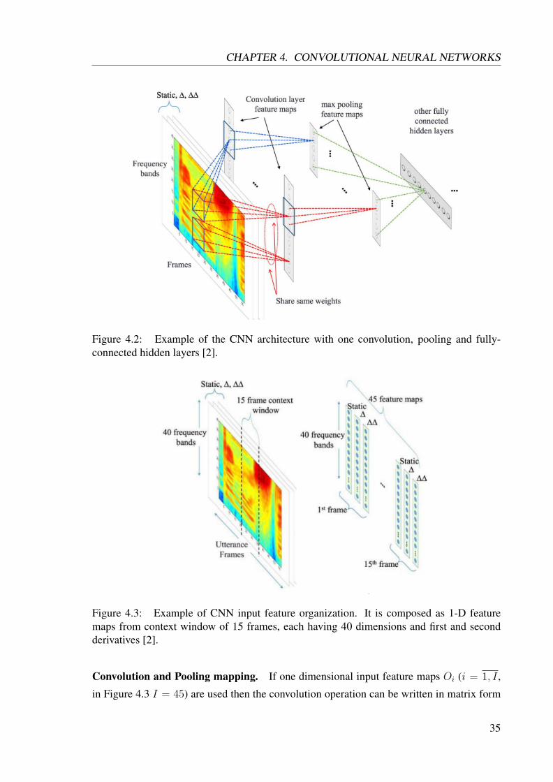
Figure 4.2: Example of the CNN architecture with one convolution, pooling and fully-connected hidden layers [2].

Figure 4.3: Example of CNN input feature organization. It is composed as 1-D featuremaps from context window of 15 frames, each having 40 dimensions and first and secondderivatives [2].

Convolution and Pooling mapping. If one dimensional input feature maps Oi (i = 1, I ,

in Figure 4.3 I = 45) are used then the convolution operation can be written in matrix form

35


using 1-D convolution mapping ∗, and it produces convolutional feature maps Qj(j = 1, J),

[2]:

Qj = σ

(I∑i=1

Oi ∗wi,j

), j = 1, J, (4.2)

where wi,j is local weight matrix (kernel), see Figure 4.4. Note that the number of feature

maps Qj in the convolution layer is corresponding to the number of weight matrices wi,j . In

practice, we will constrain many of these weight matrices to be identical. In other words,

the single feature map Qj is produced by convolving all input maps Oi with the same kernel

wi,j .

Figure 4.4: An illustration of one CNN «layer» consisting of a pair of a convolutional andpooling layers in succession, where mapping from input layer to a convolutional is based oneq. (4.2) and mapping from a convolution ply to a pooling ply is based on eq. (4.3) [2].

The max-pooling mapping can be written as in [2]

pj,m =G

maxn=1

qj,(m−1)×s+n, (4.3)

whereG is the pooling size, s is the shift size and pj,m is them-th unit of the j pooling feature

map. The pooling function is applied to every convolution map independently and consider

local region of units, the size of that region is called pooling size.

After pooling operation neural network has the same number of feature maps as the num-

ber of feature maps in its convolution layer, but each map is smaller. The purpose of the pool-

ing is to reduce the resolution of feature maps. After a sequence of convolutional-pooling

blocks signal comes to usual fully-connected feed-forward neural network. For training the

36


whole Convolutional Neural Network the backpropagation algorithm can be applied [2].

37


38

CHAPTER 5

Deep Neural Network Pre-training

5.1 Motivation for deepness

There are several hypothesis that encouraged scientists to consider neural networks to be

multilayers and have deep topology. As it was mentioned earlier in Chapter 2 that scientists

were inspired by neurophysiology in order to develop artificial neural networks, they went

further. It was proved in biology that there are many types of neurons in brain and all of

them are not chaotically connected but organize some groups and neural ensembles [35],

[16]. These neural ensembles form some levels of abstraction from primitive on the input

sensors to high levels when signal spreads further. They utilize this idea in mathematical

models of deep neural networks, see Figure 5.1.

The universal approximation theorem (Theorem 1) does not say about number of hidden

layers or units. There was the question it is better to train one layer network with many

units or deep network with less units. More formal mathematical motivation for deepness

of neural networks was proved by Y. Bengio in [10]. He showed that k + 1 - layer nets

can easily represent what a k - layer net can represent, whereas the converse is not true, i.e.

deeper networks have more generalization capacity.

Therefore, scientists were motivated to have deep topologies, but there were no training

algorithm for them. Experiments showed that training deep architectures is more difficult

than training shallow networks [11, 26]. It was suggested that supervised gradient-based

training of deep multi-layer neural networks, starting from random weights initialization,

gets stuck in local minima or plateaus [10]. When architecture gets deeper the vanishing

39

CHAPTER 5. DEEP NEURAL NETWORK PRE-TRAINING

Figure 5.1: Layers of deep neural network as a levels of brain abstractions [23]. Accordingto natural brain model of visual system the next neural layer learns new level of abstractions(e.g. dots→ dashes→ surface and lines→ objects).

gradient problem brings difficulties to obtain solution.

However, it was revealed that much better results could be archived when pre-training

each layer one by one with an unsupervised learning algorithm [40] such as the RBM gen-

erative model. After having initialized a number of layers, the whole neural network can

be fine-tuned with respect to a supervised training approach as usual. The advantage of

unsupervised pre-training versus random initialization was demonstrated in [11, 69, 86].

5.2 Deep Belief Network pre-training

In this paragraph we will see how Restricted Boltzmann Machines played important role for

whole Deep Learning [40]. Deep Belief Networks is the method which lies in the origin of

the unsupervised layer-wise pre-training for deep feed-forward networks that we have seen

before. DBN is a hybrid generative model that mixes undirected and directed connections

between units which constitute the network [40], [37].

On the Figure 5.2 example topology of DBN is presented. It has three hidden layers

marked as h and visible x. It has undirected connections between h(3) and h(2) layers and

directed between others. In DBN topology, the top two layers will always form Restricted

Boltzmann Machine network. In other words in our example the distribution p(h(2), h(3)

)is

defined by RBM with undirected connections.

40


Figure 5.2: Example of Deep Belief Network topology with three hidden layers.

Other layers form a Bayesian network instead with top-down directed interactions. Specif-

ically the conditional distributions of the units in these layers given the layer above is going

to take this form

p(h(1)j = 1

∣∣∣h(2)) = σ(b(1) +W (2)Th(2)

), (5.1)

p(x(1)j = 1

∣∣∣h(1)) = σ(b(0) +W (1)Th(1)

). (5.2)

So this corresponds to the probabilistic model associated with the logistic regression model.

That is the probability of the hidden unit h(1)j or visible unit x(1)j , which are supposed to be

equal to one, is a sigmoid applied to linear transformation of the layer above. When we have

units that interact in this way we call such a model Sigmoid Believe Network (SBN) [40].

So the Deep Belief Network is a model the top two layers form an RBM while the bottom

layers form a SBN and units are not connected with each other in one layer, only neighbor

layers are connected. In order to generate data from the DBN (see example in [36]) we would

need to do Gibbs sampling between the top two layers in the RBM for the very long time.

Once we have converge to an equilibrium distribution and h(2) is sampled from its the actual

prior distribution p(h(2), h(3)

).

Then from h(2) we would directly generate h(1) using stochastic equations (5.1) and from

h(1) we would generate directly x using (5.2). That would give us an observation or a sample

41


from the input layer x from a Deep Belief Network. It is a generative process associated with

DBN.

Notice that DBN is not a feed-forward network. Sometimes in a literature they say

«stacked RBMs are a deep belief network». If we would do that, i.e. just stacking the RBMs

and initialize a feed-forward network, we do not call this network as a deep belief network.

We would call it as unsupervised RBMs’ pre-training for feed-forward network. The DBN

is a specific model where the hidden units are stochastic and binaries and the topology is as

RBM-SBN, as it was said above.

The probabilistic model of DBN is the next the joint distribution over the input and three

hidden layers (for our example of three hidden layers)

p(x, h(1), h(2), h(3)

)= p

(h(2), h(3)

)p(h(1)∣∣h(2)) p (x|h(1)) , (5.3)

where the prier probability of h(2) and h(3) has form

p(h(2), h(3)

)= exp

(h(2)

T

W (3)h(3) + b(2)T

h(2) + b(3)T

h(3))/

Z, (5.4)

which is exactly an RBM probability function (3.5).

The probability of h(1) given h(2) is the part of the sigmoid belief network

p(h(1)∣∣h(2)) =∏

j

p(h(1)j

∣∣∣h(2)). (5.5)

Finally, we get x sampled from layer h(1)

p(x|h(1)

)=∏i

p(xi|h(1)

). (5.6)

The main fact here is that training the DBN is a hard computational problem [38]. It

turns out that a good initialization plays a crucial role on the quality of results. This is in fact

how greedy layer-wise pre-training [40] approach was developed as a way of initialization

better parameters for deep belief network. After that it was noticed that we can use same

initialization to improve training of the feed-forward neural networks. So, this is how the

idea of stacking of RBMs for pre-training came from that problem described above.

42


The idea for the initialization procedure is that in order to train three hidden layer DBN

we will start from one hidden layer DBN. One hidden layer DBN is just an RBM part of

DBN (see Figure 5.3), because we take top two layers and there are no sigmoid belief layers.

Figure 5.3: Pre-training procedure of Deep Belief Network: starts from top RBM (leftfigure), then add one by one sigmoid belief layers (central and right images) [50].

After training one hidden layer DBN we use its weights for initialization of sigmoid part

of two hidden layer DBN (Figure 5.3, central image). In two hidden layer DBN we train

again RBM part only with fixed weights for directed connections. The same idea is applied

for three hidden layers DBN, initialize and fix low part and train only top two layer RBM.

After that pre-training procedure we are doing fine-tuning.

The formal idea is that when we train one hidden layer DBN (RBM) we have a model

p (x) =∑h(1)

p(x, h(1)

), (5.7)

which is a marginalization of the hidden layer, which is defined by an RBM.

The part p(x, h(1)) we can represent as

p(x, h(1)

)= p

(x|h(1)

)p(h(1)) = p

(x|h(1)

)∑h(2)

p(h(1), h(2)

), (5.8)

when we are passing from one hidden layer to two hidden layers we fix parameters of the

p(x|h(1)

)part and train the prier part p(h(1)). For p(h(1)) we use new RBM which repre-

sented as a probability marginalized over h(2).

43


Then we repeat this procedure for three hidden layers DBN and represent p(h(1), h(2)

)as

p(h(1), h(2)

)= p

(h(1)∣∣h(2)) p (h(2)) = p

(h(1)∣∣h(2))∑

h(3)

p(h(2), h(3)

). (5.9)

This is basic idea behind stacking of RBMs in the context of the Deep Belief Networks.

In general, procedure of RBMs stacking can be repeated as many time as needed. It pro-

duces many layers of non-linear feature detectors that represent progressively more complex

statistical structure in the data. That is it was noticed that RBMs layer sequence describes

different abstraction levels from primitive to more structured.

5.3 Fine-tunning

Stacking of RBMs (or greedy layer-wise) pre-training gives just good first estimation (start-

ing point) for further fine-tunning. For fine-tunning after pre-training they usually use the

Up-Down algorithm for generative models [40] (as Deep Belief Networks) or backpropaga-

tion for discriminative training.

Notice: unfortunately, a deep neural network that is pre-trained generatively as a Deep

Belief Network, using stack of RBMs, is often still called a Deep Belief Network in the liter-

ature, for clarity see [42, 24]. Technically, it is just the same pre-training approach which

is applied for initializing weights of feed-forward network and there is nothing else general

with DBN. For clarity they call such a pre-trained networks as DBN-DNN [42].

In this work we are applying discriminative backpropagation fine-tunning. Thus after

pre-training a stack of RBMs, we «forget about the whole probabilistic framework» and use

the generative weights as initialization for deterministic feed-forward multilayer perceptron

(MLP) [42]. On the Figure 5.4 you can see that connections of multilayer perceptron has

reversed direction and on top of that we add final softmax layer and train the whole DNN

discriminatively. In this work, instead of softmax layer we will use sigmoid layer and mean

square error rate loss function.

44


Figure 5.4: Three stacked RBMs on the left figure are used as initialization for feed-forwardneural network (or so called DBN-DNN) with three hidden layers. As output layer it couldbe softmax or layer with sigmoid units that output signals one per each attribute label. TheDBN-DNN is then discriminatively fine-tuned by backpropagation to predict the attributelabel.

45


46

CHAPTER 6

Application Neural Networks for Attribute Detection

Speech attributes in natural speech are composed of overlapping several sound events. It

means that several attributes may occur at the same time [56, 59, 80]. The goal of this work

is to train system which is able to detect every attribute event occuring at any instance of the

speech recordings. In this chapter we present frame-based data-driven techniques for speech

attributes detection.

The system is implemented using two independent deep neural networks. One of the

DNN is for modeling Manner attributes and other is for Place attribute detectors. Moreover

for place and manner attributes we investigate two types of deep neural networks, these are

DBN-DNN and CNN. We tried to optimize these for the corpora and task by varying number

of hidden units and hidden layers and define the best topology.

6.1 System Overview

The problem of the attribute extraction from the speech can be treated as a multi-label de-

tection [65, 94]. Here multi-label task means that each attribute example can be associated

with multiple labels (classes). Therefore, if the size of the label set is N , multi-label detector

can associate an example with 2N different label vectors in general case. The Detection task

means that we measure probability (or score) that observation belongs to the attribute class.

This task is formally described as the automatic speech attribute transcription (ASAT)

framework [56]. It is bottom-up detection-based framework, where speech attributes are

47

CHAPTER 6. APPLICATION NEURAL NETWORKS FOR ATTRIBUTE DETECTION

extracted using data-driven modeling techniques. The goal of each detector is to analyze a

speech segment and produce a confidence score or posterior probability that pertains to some

acoustic-phonetic attribute. Attributes should be stochastic in nature. Each attribute detector

should output probabilities of target class i, non-target and noise model, given a speech frame

f : p(H

(i)target

∣∣∣ f), p(H

(i)anti

∣∣∣ f) and p(H

(i)noise

∣∣∣ f). All these probabilities sum up to one, see

Figure 6.1.

On this earlier front-end stage of the system we do not need hard decisions from the

attribute detectors because of two reasons. First reason, these detectors’ outputs will form a

new feature vector x by concatenating each of these posterior probabilities from each target

classes (7 for manners or 11 for places)[56]. These posterior vectors may be utilized then

as a high level features in other components of the system. The second reason, it shifts the

responsibility for making decisions on other components which may effectively adjust the

risk parameters and introduce additional information for decision making [32].

The first naive idea to solve a multi-label detection problem could be to decompose it

into multiple single-label multi-class detection problems, i.e. train detectors to associate each

learning example with one of the labels [94]. A network can be trained for each possible class

and the results can be combined to get multi-label detection results. However, this method

ignores the correlation between the classes and therefore has weak expressive power [94].

In the previous works [56, 79, 80] for speech attribute extraction it was proposed a possi-

ble implementation of the ASAT framework, see Figure 6.1. It consists of two main blocks:

1) a bank of attribute detectors that can produce detection result in terms of confidence score;

and 2) an evidence merger that combines low-level events into high-level evidence, such as

phone posteriors. Then append module stacks together the outputs delivered by the detec-

tors and generate a supervector of attribute detection scores. Every attribute detector was

trained using shallow artificial neural networks (ANNs) with cross-entropy cost function and

soft-max output layer, hence, simulate the posterior probabilities given the speech frame.

Recently in paper [32] it was proposed promising idea of using cutting edge Deep Neu-

ral Network (DNN pre-trained with stack of RBMs) for attribute detectors modeling. All

attribute detectors are trained using single DNN and output posterior probability vector af-

ter softmax layer, this vector represents all probabilities to be assigned to attribute classes.

This model is limited because it outputs posterior probability not per each attribute detector

independently for three hypothesis (target, non-target and noise), but it assigns the maximal

probability for one class against others, i.e. it represents single-label detector. However, even

48


Figure 6.1: Previous attribute detectors’ system architecture described in [56]. Every at-tribute implemented as an artificial neural networks, the outputs are posterior probabilitiesof a target class i, non-target and noise model, given a speech frame f : p

(H

(i)target

∣∣∣ f),

p(H

(i)anti

∣∣∣ f) and p(H

(i)noise

∣∣∣ f). All these probabilities sum up to one.

such a limited model has improved results in Foreign Accent Recognition problem [32].

In this research we represent extended idea of the previous work. Here we also use

single DNN which model all attribute detectors and produce detection result in terms of a

confidence score. We archive that replacing Cross-entropy cost function with Mean Square

Error function (MSE), the output soft-max layer is replaced with sigmoid layer. As a re-

sult in our proposed system the output scores are not probabilities, but some «posterior»

scores which measure the appearance of each attribute independently: s(Nasals|O(t)),s(Fricatives|O(t)), e.t.c. These scores are in range [0, 1] and produced by the sigmoid

units in the output layer of neural network.

In training phase input vector for the DNNs is the concatenated context of speech frames,

see Section 6.3. The target output label vector is a binary vector which determined by the

manual annotation from OGI dataset (see Section 7.1), its dimension is equal to the number

of attribute classes (Manner or Place attributes). If an attribute is annotated as present in

data transcription then the corresponding attribute class is marked with 1 in the target output

vector, otherwise it is marked with 0. During training the output sigmoid units tried to fit the

49


target label vector using MSE cost function. In testing phase the data is forwarded trough the

DNN and produce the confidence scores on the output layer. Thus multi-label detection was

solved. These raw output sigmoid scores are directly utilized further in other blocks of the

system, however these could be calibrated as discussed in [17].

6.2 Speech Feature Extraction

It is conventional in pattern recognition that before training any speech model we need to

make a signal preprocessing, extract mostly representative features and reduce the dimen-

sionality to increase computational performance [14]. Such a features are usually represented

in time-frequency space.

Here for Neural Networks we extract speech feature vectors of mean-normalized log-

filter banks: their static, first and second order derivatives [2], [32]. For extracting log-filter

banks it is needed to accomplish usual chain of signal processing. The feature vector was

extracted from 25ms sliding window with 10ms shifting using Hamming windowing. After

that we apply discrete Fourier transformation on every frame and, finally, logarithm of mel-

scale filter bank is applied to power spectrum. Typically, filter banks of 15 to 45 filters are

applied to cover the whole frequency range. For DBN-DNN 15 filters were applied, but for

CNN 40 filter banks were extracted.

Often in recent literature about DNNs [2, 73, 46] authors directly use log mel-frequency

spectral coefficients (filter banks) without a decorrelating discrete cosine transformation

(DCTs), it produces an artifacts on the decorrelated mel-frequency cepstral coefficients (MFCC)

[2]. Also as it was noticed in Section 4.2, filter bank features after DCT projection may not

maintain locality nor along the frequency neither time axis.

Figure 6.2: Spectrogram of log-filter bank features (15 filters are applied).

50


6.3 System Settings

We investigate two types of neural networks to solve the problem of attribute detection.

The first Deep Network is simple Feed-Forward neural network using Restricted Boltzmann

Machine pre-training (context-dependent DBN-DNN, see Chapter 3), the second is Convo-

lutional Neural Network. All experiments are conducted under the context-dependent DNN

to extract attribute scores per speech frame

6.3.1 DBN-DNN topology

The input feature vector for DBN-DNN is a 45-dimension mean-normalized log-filter bank

features with up to second-order derivatives and a context window of 11 frames, forming

an input vector of 495-dimension (45 × 11). The number of output classes are equal to 7

for manner, and 11 for place. Indeed, the «other» output class is added to both DNN to

handle possible unlabelled frames. DNN topologies with 512 and 1024 number of units

were studied, number of hidden layers is varying from 1 up to 10 (in total 20 DBN-DNN

topologies).

All DBN-DNN topologies are initialized with the stacked Restricted Boltzmann ma-

chines using layer by layer generative pre-training, as it was described in Section 5.2. The

pre-training algorithm is Contrastive Divergence with 1-step of Markov Chain Monte Carlo

sampling (CD-1). The first RBM has Gaussian-Bernoulli units and trained with initial learn-

ing rate of 0.01. The following RBMs have Bernoulli-Bernoulli units and a learning rate of

0.4.

After pre-training the weights and stacking all the layers, the final output Sigmoid layer

was concatenated with the DNN (see Figure 6.3). The number of output units corresponds

to the number of classes (manner or place), these are producing the attribute output scores.

The fine-tunning for final weights training is done by mini-batch Stochastic Gradient Decent

with learning rate of 0.0008. Mini-batch size is equal to 128 observations. The Mean Square

Error objective function was optimized during fine-tunning. In the DNN all Sigmoid hidden

units were used. Notice, all settings and parameters are conventional in speech community

[42]. During training we did not use momentum or regularization, all training parameter

were tracked using RBM guideline by G. Hinton [43].

51


Figure 6.3: DBN-DNN topology settings.

6.3.2 Convolutional Neural Networks topology

As shown in Figure 6.4, a 1-D CNN topology, which was trained to detect manner or place

attributes, takes input feature maps. These feature maps are organized (as in Figure 4.3)

from 40-dimensional log-Mel filter bank features and their first and second-order derivatives,

context window is size of 11 frames. In total 3 × 11 = 33 input feature maps to which we

apply 1-D convolution mapping along the frequency axis. The CNN consists of convolutional

layer and max-pooling layer, then from 1 up to 10 fully-connected hidden layers each of them

has 512 or 1024 sigmoid units.

Similar to the DBN-DNN settings in case of the CNN we optimize Mean Square Error

cost function. Output layer has sigmoid units and produces sigmoid output «posterior» scores

for every attribute (7 for manner or 11 for place) per each speech frame.

Convolutional layer in the CNN has 128 feature maps, each of which has size of 33

frequency bands, i.e. these are produced by convolving each input feature map with the filter

size of 8 (1 + (40 − 8) = 33). After that max-pooling layer outputs the maximum values

over a non-overlapping window covering the outputs of every three frequency bands in each

feature map (i.e. pooling size is 3), down-sampling the overall convolutional layer output to

three times smaller. Then the output of the max-pooling layer are fed to the fully-connected

feed-forward part of the CNN. This CNN architecture follows conventional configurations

used in the speech community [73, 46].

52


Figure 6.4: Convolutional Neural Network topology settings [46].

53


54

CHAPTER 7

Experiments and Results

7.1 Dataset

In all experiments the «stories» part of the OGI Multi-language telephone speech corpus

[64] was used to train the attribute detectors. This corpus has phoneme transcriptions (with

its start and end time in the recordings) for six languages: English, German, Hindi, Japanese,

Mandarin, and Spanish. Data from each language were pooled together to obtain around 6

hours of training, 2.5 hours of test and 0.5 hours of cross validation (cv) datasets. Sample

rate is 8kHz.

In this work it was used 7 manner of articulation classes: fricative, glide, nasal, silence,

stop, voiced, vowel; and 10 place of articulation classes: coronal, dental, glottal, high,

labial, low, mid, palatal, silence, and velar [80]. Additional class of «other» was added in

manner and place, representing any noise or unknown sound events.

Speech attributes can be obtained for a particular language and shared across many dif-

ferent languages, and they can thereby be used to derive a universal set of speech units.

Furthermore, data sharing across languages at the attribute level is naturally facilitated by

the nature of these classes as shown in [77].

In [78], the authors have demonstrated that manner and place of articulation attributes

can compactly characterise any spoken language along the same lines as in the automatic

speech attribute transcription (ASAT) paradigm for ASR [56]. Furthermore, it was shown

that off-the-shelf data-driven attribute detectors built to address automatic language iden-

55

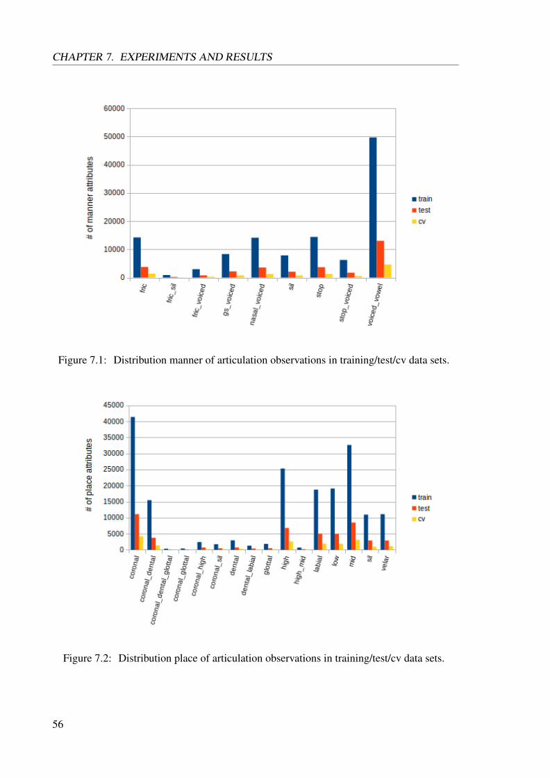
CHAPTER 7. EXPERIMENTS AND RESULTS

Figure 7.1: Distribution manner of articulation observations in training/test/cv data sets.

Figure 7.2: Distribution place of articulation observations in training/test/cv data sets.

56


tification tasks [80] can be exploited without either acoustic adaptation or re-training for

characterising speaker accents never observed before [8].

As it was mentioned above the OGI corpus has phoneme transcriptions. In order to train

attribute detectors the manner or place transcription were needed, these were obtained from

the phoneme transcriptions. We mapped phoneme transcription into corresponding manner

or place attributes transcription using mapping tables (Appendix A and B) across all of the

languages.

Whenever one phoneme belongs to several attribute classes at the same time we get

multiple attribute labels, which names are splitted with underscore (e.g. «fric_voiced»). In

other words, it means that these attributes are occurring simultaneously in the speech, and

in training target label vector these will be marked with 1 (e.g. for manner of articulation

«fric_voiced» will be [10000010] target vector). In testing phase, thanks to sigmoid output

layer in neural networks, we can get individual scores in range of (0, 1) which may assign

any input observation to multiple attribute classes, as it was discussed in Section 6.1.

Corresponding statistics of the OGI dataset are shown on Figure 7.1 and 7.2. It rep-

resents distribution of manner and place observations. Single-label as well as multi-label

observations are shown.

7.2 Performance measure

Visual inspection of the detection error tradeoff (DET) curves [60] and equal error rate

(EER) are commonly used evaluation tools for assessing the performance of the models.

DET graph shows the tradeoff between two error types: missed detections and false alarm

for different values of the threshold, using standard normal deviate axis scale. When there

is a tradeoff of error types, a single performance number is inadequate to represent the capa-

bilities of a system. Such a system has many operating points, and is best represented by a

performance curve [60]. The Equal Error Rate (EER) measure is used to summarize the per-

formance of a system, defined as the point along the DET curve where the missed detections

and false alarm are equal. This may be of use in applications where the cost of each type of

error is equal. The lower the number of EER is, the better the system performs.

57


7.2.1 DET curves

In Figure 7.3, as an example, the DET curves for fricative and voiced manner detectors are

presented. One curve on the plot representing detector performance with certain DNN topol-

ogy, in total 40 different DNN topologies were investigated. The closer curve to the origin

the better performance of the corresponding system. On both images it is noticeable that

CNN topologies outperform DBN-DNNs. The property of the DET curve is that if resulting

curve is close to straight line, then this provides a visual confirmation that the likelihood

distributions (for targets and non-targets) from the system are normal. The resulting DET

curves for fricative detector are approximately straight lines, whereas the voiced detector

curves have the shapes close to convex hyperbolic function and the closest point to the origin

is around (8,8).

In Figure 7.4 the velar place detector performance across different models is shown.

Here the resulting curves of DBNs and CNNs topologies are densely lying. But still it can be

recognized that some CNN curves are closer to the origin, thus outperform DBNs on the all

critical operating region. All of the place detectors DET plots have approximately straight

performance curves.

7.2.2 Average Equal Error Rate

Average Equal Error Rate (AvgEER) is calculated across all manner and place articulatory

detectors and for every particular neural networks model. The average error rate for manners

is depicted in Figure 7.5 and depends on the number of hidden layers and number of units.

The striking feature to note on the plot is that the CNN models detect attributes better then

DBN neural networks, on the whole variety number of hidden layers. Also with increasing

number of hidden layers the AvgEER for CNNs does not change that much from 1 to 5 layers,

it is around 11.55% for both number of units (512 or 1024). After 5 hidden layers the error

for CNNs is gradually increasing and reaching near 12.15% for CNN_512 and CNN_1024

with 10 hidden layers. In general, the number of units in CNN models does not affect the

error, the AvgEER approximately the same either for CNN_512 or CNN_1024, except for

the CNN_1024 with 8 hidden layers. We suppose that this is occasional misleading result.

58


Figure 7.3: Detection Error Tradeoff of «fricative» and «voiced» as an example of mannerdetectors using different DNN topologies: CNN with 512 or 1024 hidden units along thehidden layers from 1 up to 10, the same variety of hidden layers and units for DBN-DNN.

59


Figure 7.4: Detection Error Tradeoff of «velar» as an example of place detectors usingdifferent Deep Network topologies: CNN with 512 or 1024 hidden units along the hiddenlayers from 1 up to 10, the same variety of hidden layers and units for DBN-DNN.

Figure 7.5: Average EER across all manner attribute detectors.

60


In case of the DBN models for manner detectors we see the opposite behavior (compare

the CNNs): when the number of layers increase the error rate is gradually decreasing from

1 to 8 layers and after that increasing. There is clear gap between DBNs with 1024 and 512

units, the more number of units the better detector classify attributes. It can be noticed that

DBN-DNN as well as CNNs models are stable, their errors vary within 1% or less.

Figure 7.6: Average EER across all place attribute detectors.

In Figure 7.6 the AvgEER for place of articulatory detectors is plotted. The relation

between CNNs and DBNs topologies remains the same as in manner case, i.e. the CNN

models outperform the DBN across the whole range number of layers, except topology with

10 layers. The CNNs error rate for models with 1 up to 6 hidden layers fluctuates near

14.3%. The error of CNN topologies with more than 6 layers dramatically increases and

reach a value of 16.58%. Similar to manners, the number of units in CNN models does

not affect the error rate that much, it is hard to say which topology is better CNN_512 or

CNN_1024, their AvgEERs are pretty close to each other. It is noticeable that DBNs with

more units works better. It is clear positive tendency in DBN models: adding more hidden

layers gradually improve the accuracy.

In Tables 7.1 and 7.2, we summarize the result DNN models of the articulatory attribute

detectors, which show the lowest value of the AvgEER. Compare the performance of DNNs

vs CNNs using DET plots and AvgEER, CNNs consistently outperform DNNs across dif-

ferent variety of tuned parameters; producing 18.8% relative error reduction for manner and

61


Table 7.1: Best models of manner detectors, which trained on OGI-TS corpus, with DBN-DNNs or CNNs with hidden layers from 1 up to 10 and 512 or 1024 units in each layer.

Topology # of hid. layers AvgEER, %CNN_512 5 11.54CNN_1024 2 11.46DBN-DNN_512 8 14.45DBN-DNN_1024 2 14.11

Table 7.2: Best models of place detectors, which trained on OGI-TS corpus, with DBN-DNNs or CNNs with hidden layers from 1 up to 10 and 512 or 1024 units in each layer.

Topology # of hid. layers AvgEER, %CNN_512 3 14.06CNN_1024 3 14.19DBN-DNN_512 4 15.86DBN-DNN_1024 8 15.65

10.3% for place compare with the best DBN-DNN models. This is consistent with our expec-

tation that CNNs have better generalization ability than DNNs especially when the amount of

training data are limited [46], this idea can be confirmed by the EER plots for every manner

and place detector (see Appendix C).

7.2.3 Visualization of trained weights

Figure 7.7 shows several examples of the spectral filters (1-D convolutional kernels) learned

by the convolutional layer of the CNN. The vertical dimension represent 8 weights of the

convolutional kernel along the frequency axis, horizontal dimension represents 33 output

neurons in the convolutional feature map. These filters look like 2-D Gabor filters [46] in

varying directions: horizontal, vertical and diagonal filters.

Figure 7.7: CNN spectral filters of size 8×33 learned by the convolutional layer.

62


In Figure 7.8 the DBN-DNN weights are depicted. These weights are trained by DBN-

DNN with 2 hidden layers each of them has 1024 units. The weights, which are plotted, are

connecting the last layer with 8 outputs and previous layer with 1024 units, thus we have 8

images of weights reshaped as 32×32 matrices. There is no such a clear structure on the

images as for CNN filters, but these weight plots are used to visualize the convergence and

anomaly of the training algorithm. If there are too much black or white pixels on the weight

plots, it means that weights are very close to 0 or 1, i.e. too large or too small, that is not

natural for DBN-DNN [92].

Figure 7.8: DBN-DNN weights between last layer with 8 units and previous layer with 1024

units. These are reshaped in 32×32 matrices.

63


64

CHAPTER 8

Conclusions

In this thesis it was proposed a promising model for speech attribute detection. Two models

based on the cutting edge deep neural networks were compared. These are Convolutional

Neural Networks (CNN) and feed-forward neural networks pre-trained with the stack of

Restricted Boltzmann Machines (DBN-DNN). The proposed model is more related to the

stochastic nature of the speech articulatory attributes, than that in paper [32]. Attribute de-

tection can be considered as the multi-label detection problem, which was solved with the aid

of our model. All experiments have been conducted on the multi-language OGI-TS speech

dataset.

In order to find out the DNN model parameters for highest accuracy, many experiments

have been conducted. The effect of number of hidden fully-connected layers and number of

units were investigated. In order to measure the systems’ performance on the test dataset and

compare the models in general, several evaluation metrics were chosen. The DET curves

approach in general and AvgEER (in Figures 7.5 and 7.6) in particular, consistently show

that manner and place articulatory detectors trained with the CNN models work better than

DBN-DNN models. The CNNs, compare with the DBN-DNNs, provide a significant error

reduction producing 18.8% for manner and 10.3% for place relative AvgEER improvements

(see Tables 7.1 and 7.2). Also tendency that CNNs outperform DBN-DNNs across differ-

ent test parameters is confirmed by EER plots for every detector (see Appendix C). More-

over, manner speech features are detected more accurately then place features 11.46% versus

14.06% AvgEER, taking the best topologies.

The lowest AvgEER have been shown for manners by CNN with 2 hidden fully-connected

layers each has 1024 units, for places the best results were obtained by CNN with 3 hidden

65

CHAPTER 8. CONCLUSIONS

layers and each of them had 512 units. Both CNN topologies has single convolutional and

max-pulling layers.

From our experiments we can conclude that detectors trained with CNN models have

better generalization ability than DBN-DNNs especially when the amount of training data

is limited, as in our case we have very biased number of observations. It was shown (in

Figure 7.7) that a CNN with random initialization can automatically learn various sets of

edge detectors to locally extract low-level speech features. From the EER figures it can be

concluded that CNN models suffer from overtraining, whenever we add more hidden fully-

connected layers the error rate dramatically increases. In case of DBN-DNN we see the

opposite behavior. Thus, we may conclude that stacking of RBMs or layer-wise pre-training

gives gradual improvements of the model with the increase of hidden layers.

The next direction of the research is to apply multi-task learning approach as the infer-

ence framework above deep neural networks. Another investigation will be concerning the

application of speech articulatory attributes in speaker recognition problem.

66

Bibliography

[1] The nobel prize in physiology or medicine 1906. nobelprize.org. nobel media ab 2014.

[2] Ossama Abdel-Hamid, Abdel rahman Mohamed, Hui Jiang, Li Deng, Gerald Penn, and

Dong Yu. Convolutional neural networks for speech recognition. IEEE/ACM TRANS-

ACTIONS ON AUDIO, SPEECH, AND LANGUAGE PROCESSING, October 2014.

[3] Ossama Abdel-Hamid, Abdel rahman Mohamed, Hui Jiang, and Gerald Penn. Ap-

plying convolutional neural networks concepts to hybrid NN-HMM model for speech

recognition. In 2012 IEEE International Conference on Acoustics, Speech and Signal

Processing (ICASSP). IEEE, mar 2012.

[4] P. Angkititrakul and J. H.L. Hansen. Advances in phone-based modeling for automatic

accent classification. Trans. Audio, Speech and Lang. Proc., 14(2):634–646, December

2006.

[5] Levent M. Arslan, John H. L. Hansen, Prof John, and H. L. Hansen. Language accent

classification in american english, 1996.

[6] J. Baker, L. Deng, J. Glass, S. Khudanpur, C. H. Lee, N. Morgan, and

D. O’Shgughnessy. Research developments and directions in speech recognition and

understanding. IEEE Signal Processing Magazine, 26(3):75–80, 2009.

[7] Erwin H. Bareiss. Numerical solution of linear equations with toeplitz and vector

toeplitz matrices. Numer. Math., 13(5):404–424, oct 1969.

[8] Hamid Behravan, Ville Hautamauki, Sabato Marco Siniscalchi, Tomi Kinnunen, and

Chin-Hui Lee. Introducing attribute features to foreign accent recognition. In 2014

IEEE International Conference on Acoustics, Speech and Signal Processing (ICASSP).

Institute of Electrical & Electronics Engineers (IEEE), may 2014.

67

BIBLIOGRAPHY

[9] Jacob Benesty, M. Mohan Sondhi, and Yiteng (Arden) Huang. Springer Handbook of

Speech Processing. Springer-Verlag New York, Inc., Secaucus, NJ, USA, 2007.

[10] Y. Bengio. Learning deep architectures for AI. Foundations and Trends R© in Machine

Learning, 2(1):1–127, 2009.

[11] Y. Bengio, P. Lamblin, D. Popovici, and H. Larochelle. Greedy layer-wise training of

deep networks. In In NIPS, 2007.

[12] Yoshua Bengio, Ian J. Goodfellow, and Aaron Courville. Deep learning. Book in

preparation for MIT Press, 2015.

[13] Yoshua Bengio, Yann Lecun, and Yann Lecun. Convolutional networks for images,

speech, and time-series, 1995.

[14] Christopher M. Bishop. Pattern Recognition and Machine Learning. Springer, 2006.

[15] Ronald Bracewell. The Fourier Transform & Its Applications. McGraw-Hill, 1965.

[16] Amy Brisben, Miguel Nicolelis, Mark Laubach, and Christopher Stambaugh. Methods

for Simultaneous Multisite Neural Ensemble Recordings in Behaving Primates. In-

forma UK Limited, dec 1998.

[17] Niko Brummer. Measuring, refining and calibrating speaker and language information

extracted from speech. PhD thesis, University of Stellenbosch, 2010.

[18] M. A. Carreira-Perpinan and G. E. Hinton. On contrastive divergence learning. Pro-

ceedings of the Tenth International Workshop on Artificial Intelligence and Statistics

(AISTATS’05), pages 33–40, 2005.

[19] M. A. Carreira-Perpinan and G. E. Hinton. Proceedings of the Tenth International

Workshop on Artificial Intelligence and Statistics, Jan 6-8, 2005, Savannah Hotel, Bar-

bados, chapter On Contrastive Divergence Learning, pages 33–40. 2005.

[20] A. H. Carter. Classical and Statistical Thermodynamics. Prentice Hall, New Jersey,

2001.

[21] A. Coates, H. Lee, and A. Y. Ng. An analysis of single-layer networks in unsupervised

feature learning. International Conference on Artificial Intelligence and Statistics (AIS-

TATS), 2011.

68

BIBLIOGRAPHY

[22] G. Cybenko. Approximations by superpositions of sigmoidal functions. Mathematics

of Control, Signals, and Systems, 2(4):303–314, 1989.

[23] J. Dean. Large scale deep learning, April 2015. Available at http:

//static.googleusercontent.com/media/research.google.

com/ru//people/jeff/CIKM-keynote-Nov2014.pdf [Online; accessed

9-June-2015].

[24] Li Deng. Three classes of deep learning architectures and their applications: A tutorial

survey. APSIPA Transactions on Signal and Information Processing, 2012.

[25] Li Deng and Dong Yu. Deep learning: Methods and applications. Found. Trends Signal

Process., 7(3–4):197–387, June 2014.

[26] Dumitru Erhan, Pierre-Antoine Manzagol, Yoshua Bengio, Samy Bengio, and Pascal

Vincent. The difficulty of training deep architectures and the effect of unsupervised pre-

training. In Twelfth International Conference on Artificial Intelligence and Statistics

(AISTATS), pages 153–160, 2009.

[27] T. S. Ferguson. An inconsistent maximum likelihood estimate. Journal of the American

Statistical Association, 77(380):831–834, 1982.

[28] Sadaoki Furui. Digital speech processing, synthesis, and recognition. Signal processing

and communications. Marcel Dekker, New York, 2001.

[29] Silke Goronzy, Stefan Rapp, and Ralf Kompe. Generating non-native pronunciation

variants for lexicon adaptation. Speech Communication, 42(1):109–123, jan 2004.

[30] Thomas Steele Hall. Treatise of Man by Rene Descartes. French text with translation

and commentary. Harvard University Press, Cambridge, Massachusetts, 1972.

[31] John H.L. Hansen and Levent M. Arslan. Foreign accent classification using source

generator based prosodic features. In Proc. ICASSP, pages 836–839. IEEE, 1995.

[32] V. Hautamaki, S. M. Siniscalchi, H. Behravan, V. M. Salerno, and I. Kukanov. Boosting

universal speech attributes classification with deep neural network for foreign accent

characterization. 2015.

[33] S. O. Haykin. Neural Networks and Learning Machines. 3 edition, 2008.

[34] Kaiming He, Xiangyu Zhang, Shaoqing Ren, and Jian Sun. Delving deep into rectifiers:

Surpassing Human-Level performance on ImageNet classification, February 2015.

69

http://static.googleusercontent.com/media/research.google.com/ru//people/jeff/CIKM-keynote-Nov2014.pdf



BIBLIOGRAPHY

[35] Donald O. Hebb. The Organization of Behavior. New York: Wiley & Sons, 1949.

[36] G. Hinton. Deep belief network trained on mnist, example in action. Available

at http://www.cs.toronto.edu/~hinton/adi/index.htm [Online; ac-

cessed 9-June-2015].

[37] G. Hinton. Deep belief networks. Scholarpedia, 4(5):5947, 2009.

[38] G. Hinton, P Dayan, B. Frey, and R. Neal. The "wake-sleep" algorithm for unsupervised

neural networks. Science, 268(5214):1158–1161, may 1995.

[39] G. E. Hinton. Training products of experts by minimizing contrastive divergence. Neu-

ral Computation, 14(8):1771–1800, aug 2002.

[40] G. E. Hinton, S. Osindero, and Y. Teh. A fast learning algorithm for deep belief nets.

Neural Computation, 18(7):1527–1554, 2006.

[41] G. E. Hinton and R. R. Salakhutdinov. Reducing the dimensionality of data with neural

networks. Science, 313(5786):504–507, 2006.

[42] Geoffrey Hinton, Li Deng, Dong Yu, George Dahl, Abdel rahman Mohamed, Navdeep

Jaitly, Andrew Senior, Vincent Vanhoucke, Patrick Nguyen, Tara Sainath, and Brian

Kingsbury. Deep neural networks for acoustic modeling in speech recognition: The

shared views of four research groups. IEEE Signal Process. Mag., 29(6):82–97, nov

2012.

[43] Geoffrey E. Hinton. A practical guide to training restricted boltzmann machines. In

Grégoire Montavon, Geneviève B. Orr, and Klaus-Robert Müller, editors, Neural Net-

works: Tricks of the Trade, volume 7700 of LNCS, chapter 24, pages 599–619. Springer

Berlin Heidelberg, second ed. edition, 2012.

[44] S. Hochreiter. Untersuchungen zu dynamischen neuronalen netzen. Master’s thesis,

Institut f. Informatik, Technische Univ. Munich, 1991.

[45] S. Hochreiter, Y. Bengio, P. Frasconi, and J. Schmidhuber. Gradient flow in recurrent

nets: the difficulty of learning long-term dependencies. IEEE Press, 2001.

[46] Jui-Ting Huang, Jinyu Li, and Yifan Gong. An analysis of convolutional neural net-

works for speech recognition. In ICASSP, April 2015.

[47] Sergey Ioffe and Christian Szegedy. Batch normalization: Accelerating deep network

training by reducing internal covariate shift, March 2015.

70

http://www.cs.toronto.edu/~hinton/adi/index.htm

BIBLIOGRAPHY

[48] A. N. Kolmogorov. On the representation of continuous functions of many variables by

superposition of continuous functions of one variable and addition. Doklady Akademii

Nauk SSSR, 1957.

[49] L.D. Landau and E.M. Lifshitz. Statistical Physics: Course of Theoretical Physics,

volume 5. Pergamon Press, Institute of Physical Problems USSR Academy of Sciences,

1969.

[50] H. Larochelle. Neural networks lectures, 2013. Available at http:

//info.usherbrooke.ca/hlarochelle/cours/ift725_A2013/

contenu.html [Online; accessed 9-June-2015].

[51] H. Larochelle and Y. Bengio. Classification using discriminative restricted boltzmann

machines. Proceedings of the 25th international conference on Machine learning -

ICML’08, 2008.

[52] Y. LeCun, L. Bottou, G. B. Orr, and K.-R. Muller. Efficient backprop. Neural Networks:

tricks of the trade. - Springer, 1998.

[53] Y. LeCun, S. Chopra, R. M. Hadsell, M.-A. Ranzato, and F.-J. Huang. A tutorial on

energy-based learning. MIT Press, 2006.

[54] Y. LeCun, J. Denker, S. Solla, R. E. Howard, and L. D. Jackel. Optimal brain damage.

Advances in Neural Information Processing Systems II, 1990.

[55] Y. LeCun and F. Huang. Loss functions for discriminative training of energy-based

models. Proceedings of the Tenth International Workshop on Artificial Intelligence and

Statistics (AISTATS’05), 2005.

[56] Chin-Hui Lee and Sabato Marco Siniscalchi. An information-extraction approach

to speech processing: Analysis, detection, verification, and recognition. IEEE,

101(5):1089–1115, 2013.

[57] J. Li, Y. Tsao, and Chin-Hui Lee. A study on knowledge source integration for candi-

date rescoring in automatic speech recognition. ICASSP, 2005.

[58] Jean luc Gauvain and Chin hui Lee. Maximum a posteriori estimation for multivariate

gaussian mixture observations of markov chains. IEEE Transactions on Speech and

Audio Processing, 2:291–298, 1994.

71

http://info.usherbrooke.ca/hlarochelle/cours/ift725_A2013/contenu.html



BIBLIOGRAPHY

[59] Dau-Cheng Lyu, Sabato Marco Siniscalchi, Tae-Yoon Kim, and Chin-Hui Lee. Contin-

uous phone recognition without target language training data. ISCA, 2008.

[60] A. Martin, G. Doddington, T. Kamm, M. Ordowski, and M. Przybocki. The det curve

in assessment of detection task performance. pages 1895–1898, 1997.

[61] Warren S. McCulloch and Walter Pitts. A logical calculus of the ideas immanent in

nervous activity. The bulletin of mathematical biophysics, 5:115–133, December 1943.

[62] Yajie Miao and Florian Metze. Improving low-resource cd-dnn-hmm using dropout

and multilingual dnn training. In INTERSPEECH’13, pages 2237–2241, 2013.

[63] Marvin Minsky and Seymour Papert. Perceptrons: an introduction to computational

geometry. The MIT Press, Cambridge MA, 1969.

[64] Y. K. Muthusamy, R. A. Cole, and B. T. Oshika. The OGI Multi-Language telephone

speech corpus. In Proceedings of the International Conference on Spoken Language

Processing, pages 895–898, 1992.

[65] Jinseok Nam, Jungi Kim, Eneldo Loza Mencía, Iryna Gurevych, and Johannes

Fürnkranz. Large-scale multi-label text classification - revisiting neural networks. In

Toon Calders, Floriana Esposito, Eyke Hüllermeier, and Rosa Meo, editors, Proceed-

ings of the European Conference on Machine Learning and Principles and Practice of

Knowledge Discovery in Databases (ECML-PKDD-14), Part 2, volume 8725 of Lec-

ture Notes in Computer Science, pages 437–452. Springer Berlin Heidelberg, 2014.

[66] John Nerbonne. Linguistic variation and computation (invited talk). In EACL, pages

3–10. The Association for Computer Linguistics, 2003.

[67] M. A. Nielsen. Neural Networks and Deep Learning. Determination Press, 2015.

[68] M. Ranzato, Y. Boureau, S. Chopra, and Y. LeCun. A unified energy-based framework

for unsupervised learning. Proceedings of the Eleventh International Conference on

Artificial Intelligence and Statistics (AISTATS’07), 2007.

[69] Marc’Aurelio Ranzato, Christopher Poultney, Sumit Chopra, and Yann Lecun. Efficient

learning of sparse representations with an energy-based model. In Advances in Neural

Information Processing Systems (NIPS 2006, 2006.

[70] Frank Rosenblatt. The perceptron - a perceiving and recognizing automaton. Technical

Report 85-460-1, Cornell Aeronautical Laboratory, 1957.

72

BIBLIOGRAPHY

[71] D.E. Rumelhart, G.E. Hinton, and R. J. Williams. Learning internal representations by

error propagation. Parallel distributed processing: Explorations in the microstructure

of cognition, 1, 1986.

[72] Tara N. Sainath, Brian Kingsbury, Abdel-rahman Mohamed, George E. Dahl, George

Saon, Hagen Soltau, Tomás Beran, Aleksandr Y. Aravkin, and Bhuvana Ramabhadran.

Improvements to deep convolutional neural networks for LVCSR. In 2013 IEEE Work-

shop on Automatic Speech Recognition and Understanding, Olomouc, Czech Republic,

December 8-12, 2013, pages 315–320, 2013.

[73] Tara N. Sainath, Abdel-rahman Mohamed, Brian Kingsbury, and Bhuvana Ramabhad-

ran. Deep convolutional neural networks for LVCSR. In IEEE International Conference

on Acoustics, Speech and Signal Processing, ICASSP 2013, Vancouver, BC, Canada,

May 26-31, 2013, pages 8614–8618, 2013.

[74] R. Salakhutdinov and G. Hinton. Replicated softmax: an undirected topic model. Neu-

ral Information Processing Systems, 23, 2010.

[75] R. Salakhutdinov, A. Mnih, and G. Hinton. Restricted boltzmann machines for collab-

orative filtering. Proceedings of the 24th international conference on Machine learning

- ICML’07, 2007.

[76] Frank Seide, Gang Li, and Dong Yu. Conversational speech transcription using context-

dependent deep neural networks. In Interspeech 2011. International Speech Communi-

cation Association, August 2011.

[77] S. M. Siniscalchi, Dau-Cheng Lyu, T. Svendsen, and Chin-Hui Lee. Experiments

on Cross-Language attribute detection and phone recognition with minimal Target-

Specific training data. Audio, Speech, and Language Processing, IEEE Transactions

on, 20(3):875–887, March 2012.

[78] Sabato M. Siniscalchi, Jeremy Reed, Torbjørn Svendsen, and Chin-Hui Lee. Universal

attribute characterization of spoken languages for automatic spoken language recogni-

tion. Computer Speech & Language, 27(1):209–227, January 2013.

[79] Sabato Marco Siniscalchi, Torbjorn Svendsen, and Chin-Hui Lee. Towards bottom-up

continuous phone recognition. ASRU, 2007.

[80] Sabato Marco Siniscalchi, Torbjorn Svendsen, and Chin-Hui Lee. Toward a detector-

based universal phone recognition. IEEE, 2008.

73

BIBLIOGRAPHY

[81] P. Smolensky. Chapter 6: Information processing in dynamical systems: Foundations

of harmony theory. Parallel Distributed Processing: Explorations in the Microstructure

of Cognition, 1:194–281, 1986.

[82] P. Smolensky. Information processing in dynamical systems: Foundations of harmony

theory. Parallel Distributed Processing: Explorations in the Microstructure of Cogni-

tion, 1986.

[83] Bennie G. Thompson. Border security fraud risks complicate states ability to manage

diversity visa program. GAO, 2007.

[84] R. C. Tolman. The Principles of Statistical Mechanics. Dover Publications, 1938.

[85] Yukio Tono, Yuji Kawaguchi, and Makoto Minegishi, editors. Developmental and

Crosslinguistic Perspectives in Learner Corpus Research. Tokyo University of For-

eign Studies 4. John Benjamins, Philadelphia, 2012.

[86] Pascal Vincent, Hugo Larochelle, Yoshua Bengio, and Pierre A. Manzagol. Extracting

and composing robust features with denoising autoencoders. In Proceedings of the

25th International Conference on Machine Learning, ICML ’08, pages 1096–1103,

New York, NY, USA, 2008. ACM.

[87] K.V. Voroncov. Lekcii po nejronnim setiam. 2007.

[88] Huazheng Wang, Bin Gao, Jiang Bian, Fei Tian, and Tie-Yan Liu. Solving verbal

comprehension questions in IQ test by Knowledge-Powered word embedding, May

2015.

[89] Wikipedia. Canonical ensemble — wikipedia, the free encyclopedia, 2015. Avail-

able at http://en.wikipedia.org/w/index.php?title=Canonical_

ensemble&oldid=659866755 [Online; accessed 9-June-2015].

[90] Wikipedia. Neuron — wikipedia, the free encyclopedia, 2015. Available at http://

en.wikipedia.org/w/index.php?title=Neuron&oldid=664941774

[Online; accessed 9-June-2015].

[91] Yong Xu, Jun Du, Li-Rong Dai, and Chin-Hui Lee. A regression approach to speech

enhancement based on deep neural networks. IEEE/ACM Trans. Audio, Speech and

Lang. Proc., 23(1):7–19, January 2015.

74

http://en.wikipedia.org/w/index.php?title=Canonical_ensemble&oldid=659866755

http://en.wikipedia.org/w/index.php?title=Canonical_ensemble&oldid=659866755

http://en.wikipedia.org/w/index.php?title=Neuron&oldid=664941774

http://en.wikipedia.org/w/index.php?title=Neuron&oldid=664941774

[92] Jason Yosinski and Hod Lipson. Visually debugging restricted boltzmann machine

training with a 3d example. In The Representation Learning Workshop, 29-th Interna-

tional Conference on Machine Learning, Edinburgh, Scotland, UK, 2012.

[93] D. Yu and L. Deng. Automatic Speech Recognition: A Deep Learning Approach.

Springer, London, 2015.

[94] Min-Ling Zhang. Multilabel neural networks with applications to functional genomics

and text categorization. IEEE Transactions on Knowledge and Data Engineering,

18(10):1338–1351, October 2006.

75

APPENDIX A

Manner Multi Labels mapping to Phonemes

−−− SPANISH −−−f r i c ch f hh hs hx j h s sh t h

f r i c _ v o i c e d bx dh gx

g s _ v o i c e d l l y r w y

n a s a l _ v o i c e d m n ng

s i l pau

s t o p k p t

s t o p _ v o i c e d b d g

vo iced_vowe l aa ae ah ay eh ey i h i y ow uh uw

−−− ENGLISH −−−f r i c ch f hh s sh t h

f r i c _ v o i c e d dh j h v z

g s _ v o i c e d l r w y


s i l pau

s t o p k p t

s t o p _ v o i c e d b d dx g

vo iced_vowe l aa ae ah aw ay eh e r ey i h i y ow oy uh uw

−−− HINDI −−−f r i c ch chh f hh s sh

f r i c _ v o i c e d j h z

77

g s _ v o i c e d l r w y


s i l d d c l d t c l pau

s t o p d t d t h dx k kh p rd t t h

s t o p _ v o i c e d b bh d dd dh g

vo iced_vowe l a aa ae ah a i aw e eh i h i y ow uh uw

−−− GERMAN −−−f r i c ch cx f hh s sh t s x

f r i c _ v o i c e d j h v z

g s _ v o i c e d l r y


s i l pau

s t o p dx k p t


vo iced_vowe l A: a aa ae ah a i aw ea ee eh i a i h ihw i y oa oo uh uw

−−− MANDARIN −−−f r i c c ch f hh s sh s h r t s t s h t s r

f r i c _ s i l c h c l t s c l t s r c l

f r i c _ v o i c e d v

g s _ v o i c e d l r w


s i l pau

s t o p k kh p ph t tH

vo iced_vowe l a aa ae ah a i aw eh e r ey i h i y iyw oe ow ox u uw

−−− JAPANESE −−−f r i c ch f hh s sh t s

f r i c _ v o i c e d dz j h z

g s _ v o i c e d r r r w y


s i l pau

s t o p k p t


78

vo iced_vowe l a ah ay ey i y ow uw

79

APPENDIX B

Place Multi Labels mapping to Phonemes

−−− SPANISH −−−c o r o n a l r

c o r o n a l _ d e n t a l d l n s t

c o r o n a l _ d e n t a l _ g l o t t a l hs

d e n t a l dh t h

g l o t t a l hh

h igh ch i h i y j h sh uh uw y

l a b i a l b bx f m p w

low aa ae ay

mid ah eh ey ow

s i l pau

v e l a r g gx hx k ng

−−− ENGLISH −−−c o r o n a l d dx l n s t z

d e n t a l dh t h

g l o t t a l hh

h igh ch i h i y j h sh uh uw y

l a b i a l b f m p v w

low aa ae aw ay oy

mid ah eh ey ow

s i l pau

v e l a r g k ng

81

−−− HINDI −−−c o r o n a l d dd dx l s z

c o r o n a l _ d e n t a l d t d t h n

c o r o n a l _ h i g h ch chh j h

g l o t t a l hh

h igh i h i y sh uh uw y

l a b i a l b bh f m p w

low a aa ae a i aw

mid ah eh ow

s i l d d c l d t c l pau

v e l a r g k kh ng

−−− GERMAN −−−c o r o n a l ch cx d dx l n r s t t s x z

c o r o n a l _ g l o t t a l hh

c o r o n a l _ h i g h j h sh y

c o r o n a l _ s i l pau

d e n t a l _ l a b i a l f v

h igh i h i y uw

high_mid uh

l a b i a l b m p

low A: a aa ae

mid ah ee eh oa oo

v e l a r g k ng

−−− MANDARIN −−−c o r o n a l l n

c o r o n a l _ d e n t a l s t

d e n t a l tH

g l o t t a l hh

h igh ch i h i y iyw sh s h r uw

l a b i a l f m p ph v w

low aa ae aw

mid ah eh e r ey oe ow ox

82

s i l c h c l pau t s c l t s r c l

v e l a r k kh ng

−−− JAPANESE −−−c o r o n a l _ d e n t a l d dz n s t t s z

c o r o n a l _ h i g h ch j h sh y

g l o t t a l hh

h igh i y uw

l a b i a l b f m p w

low a ay

mid ah ey ow

s i l pau

v e l a r g k ng

83

APPENDIX C

Equal Error Rate for all detectors and different Neural

Network topologies

85

Figure C.1: EER for every articulatory detector depends on variety of DBN-DNN and CNNmodels: from 1 up to 10 hidden layers and each of them with 512 or 1024 units.

87

speech attribute detection using deep learningcs.uef.fi/sipu/pub/speechatrib-kukanov.pdf · in this...

Documents