speech enhancement and noise-robust automatic speech...
TRANSCRIPT
Speech Enhancement and Noise-RobustAutomatic Speech Recognition
- Harvesting the Best of Two Worlds
Dennis A. L. Thomsen & Carina E. AndersenGroup: 15gr1071
Signal Processing and ComputingJune 3, 2015
Supervisors:Zheng-Hua Tan & Jesper Jensen
Department of Electronic Systems
Aalborg University
Fredrik Bajers Vej 7B
DK-9220 Aalborg

Department of Electronic Systems
Frederik Bajers Vej 7
DK-9220 Aalborg Ø
http://es.aau.dk
Title:
Speech Enhancement and Noise-Robust Au-
tomatic Speech Recognition - Harvesting the
Best of Two Worlds
Theme:
Signal Processing and Computing
Project period:
September 1st 2014 - June 3rd 2015
Project group:
15gr1071
Members:
Carina Enevold Andersen
Dennis Alexander Lehmann Thomsen
Supervisors:
Zheng-Hua Tan
Jesper Jensen
No. printed Copies: 3
No. of Pages: 130
Total no. of pages: 144
Attached: 1 CD
Synopsis:
This project investigates any potential re-
lationship between the performances of
noise reduction algorithms in the context
of speech recognition and speech enhance-
ment. General theory related to speech pro-
duction and hearing is presented together
with the basics of the Mel-frequency cep-
stral coefficients speech feature. The fun-
damental theory of hidden Markov model
speech recognition is stated along with the
standard feature-extraction method Euro-
pean telecommunication standards institute
(ETSI) advanced frontend (AFE). The perfor-
mance of the ETSI AFE algorithm and state-
of-the-art speech enhancement algorithms
are investigated in both fields using speech
data from the Aurora-2 database. The ag-
gressiveness of the noise reduction applied
has been identified as a major difference be-
tween the algorithms from the two fields,
and has been adjusted to increase perfor-
mance in the rivalling field. Using a logis-
tic model, estimators of recognition perfor-
mance are created for the ETSI AFE using the
distortion measures for speech quality and
intelligibility. The most accurate estimator
of the recognition performance of the ETSI
AFE, proved to be the one designed for short-
time objective intelligibility measure using
a recogniser trained with clean and noisy
speech data.
iii

Table Of Contents
Preface vii
Chapter 1 Introduction 1
1.1 Problem Statement . . . . . . . . . . . . . . . . . . . . . . . . . . . . . . . . . . . . 2
1.2 Project Scope . . . . . . . . . . . . . . . . . . . . . . . . . . . . . . . . . . . . . . . . 2
1.3 Delimitations . . . . . . . . . . . . . . . . . . . . . . . . . . . . . . . . . . . . . . . . 3
Chapter 2 Introduction to Speech Fundamentals 5
2.1 Speech Communication . . . . . . . . . . . . . . . . . . . . . . . . . . . . . . . . . 5
2.2 Characteristics and Production of Speech . . . . . . . . . . . . . . . . . . . . . . . 6
2.3 Speech Production Model . . . . . . . . . . . . . . . . . . . . . . . . . . . . . . . . 8
2.4 Hearing . . . . . . . . . . . . . . . . . . . . . . . . . . . . . . . . . . . . . . . . . . . 10
2.5 Auditory Masking . . . . . . . . . . . . . . . . . . . . . . . . . . . . . . . . . . . . . 15
2.6 Mel-frequency Cepstral Coefficients (MFCCs) . . . . . . . . . . . . . . . . . . . . 16
2.6.1 Mel-frequency Scale . . . . . . . . . . . . . . . . . . . . . . . . . . . . . . . 17
2.6.2 Short-time Frequency Analysis . . . . . . . . . . . . . . . . . . . . . . . . . 18
2.6.3 Definition and Characteristics of Cepstral Sequences . . . . . . . . . . . 20
2.6.4 Calculating Cepstral Coefficients . . . . . . . . . . . . . . . . . . . . . . . 22
2.6.5 Feature Augmentation . . . . . . . . . . . . . . . . . . . . . . . . . . . . . . 23
Chapter 3 Automatic Speech Recognition 25
3.1 ETSI Advanced Front-End . . . . . . . . . . . . . . . . . . . . . . . . . . . . . . . . 26
3.1.1 Feature Extraction . . . . . . . . . . . . . . . . . . . . . . . . . . . . . . . . 27
3.2 HMM Based Speech Recognition System . . . . . . . . . . . . . . . . . . . . . . . 33
3.2.1 ETSI Aurora-2 Task . . . . . . . . . . . . . . . . . . . . . . . . . . . . . . . . 33
3.2.2 Hidden Markov Model (HMM) . . . . . . . . . . . . . . . . . . . . . . . . . 35
3.2.3 Training . . . . . . . . . . . . . . . . . . . . . . . . . . . . . . . . . . . . . . 38
3.2.4 Recognition . . . . . . . . . . . . . . . . . . . . . . . . . . . . . . . . . . . . 40
3.3 Performance Evaluation Methods . . . . . . . . . . . . . . . . . . . . . . . . . . . . 42
Chapter 4 Speech Enhancement 45
4.1 Iterative Wiener Filtering . . . . . . . . . . . . . . . . . . . . . . . . . . . . . . . . . 46
v
4.2 Audible Noise Suppression . . . . . . . . . . . . . . . . . . . . . . . . . . . . . . . . 51
4.3 Statistical Model Based Methods . . . . . . . . . . . . . . . . . . . . . . . . . . . . 55
4.3.1 Bayesian Estimator Based on Weighted Euclidean Distortion Measure . 56
4.4 Noise Power Spectrum Estimation . . . . . . . . . . . . . . . . . . . . . . . . . . . 60
4.5 Performance Evaluation Methods . . . . . . . . . . . . . . . . . . . . . . . . . . . . 61
4.5.1 Short-Time Objective Intelligibility (STOI) Measure . . . . . . . . . . . . 61
4.5.2 Perceptual Evaluation of Speech Quality (PESQ) . . . . . . . . . . . . . . 63
Chapter 5 Speech Enhancement using ETSI AFE 67
5.1 Extracting Denoised Speech Signals from ETSI AFE . . . . . . . . . . . . . . . . . 67
5.2 Comparison of Speech Quality Measurements . . . . . . . . . . . . . . . . . . . . 70
5.3 Comparison of Speech Intelligibility Measurements . . . . . . . . . . . . . . . . . 73
5.4 Comparisons of Spectrograms using ETSI AFE vs. STSA WE . . . . . . . . . . . . 75
5.5 Adjustment of Aggressiveness . . . . . . . . . . . . . . . . . . . . . . . . . . . . . . 77
5.6 Discussion . . . . . . . . . . . . . . . . . . . . . . . . . . . . . . . . . . . . . . . . . 79
Chapter 6 ASR using Speech Enhancement Pre-processing Methods 81
6.1 ASR Results . . . . . . . . . . . . . . . . . . . . . . . . . . . . . . . . . . . . . . . . . 82
6.2 Adjustment of Aggressiveness . . . . . . . . . . . . . . . . . . . . . . . . . . . . . . 85
6.3 Frame Dropping by the use of Reference VAD Labels . . . . . . . . . . . . . . . . 88
6.4 Discussion . . . . . . . . . . . . . . . . . . . . . . . . . . . . . . . . . . . . . . . . . 90
Chapter 7 Correlation of ASR and Speech Enhancement Performance Measures 93
7.1 Correlation Coefficients . . . . . . . . . . . . . . . . . . . . . . . . . . . . . . . . . 95
7.1.1 Pearson Correlation Coefficient . . . . . . . . . . . . . . . . . . . . . . . . 95
7.1.2 Spearman Rank Correlation Coefficient . . . . . . . . . . . . . . . . . . . 96
7.1.3 Kendall Tau Rank Correlation Coefficient . . . . . . . . . . . . . . . . . . . 97
7.2 Impact of Blind Equalization on Correlation Between STOI/PESQ Scores and
ASR Results . . . . . . . . . . . . . . . . . . . . . . . . . . . . . . . . . . . . . . . . . 98
7.3 Correlation Between ASR and SE Performance Measures using ETSI AFE . . . . 101
7.3.1 Correlation of STOI Measure with ASR Measures . . . . . . . . . . . . . . 101
7.3.2 Correlation of PESQ Measure with ASR Measures . . . . . . . . . . . . . . 106
7.3.3 Estimation of the ETSI AFE Recognition Performance . . . . . . . . . . . 110
7.4 Correlation Across Feature Extraction Algorithms . . . . . . . . . . . . . . . . . . 114
7.5 Discussion . . . . . . . . . . . . . . . . . . . . . . . . . . . . . . . . . . . . . . . . . 118
Chapter 8 Conclusion 121
References 123
A Settings 127
vi

B Matlab Scripts 129
vii

Preface
This master thesis presents the final project of the Master of Science in Signal Processing and
Computing at Aalborg University. The project has been prepared by project group 15gr1071 at
the Institute of Electronic Systems between September 2014 and June 2015. The project has
been done in collaboration with Oticon and has been supervised by Jesper Jensen and Zheng-
Hua Tan.
The formatting should be interpreted as follows:
• Figures, tables, equations and algorithms are numbered consecutively according to the
chapter number.
• Citations are written with indicies in squared brackets, i.e. [i ndex].
• The enclosed CD contains a digital copy of this thesis, Matlab scripts and software used
to perform feature extraction and speech recognition.
Aalborg University, June 3, 2015
Carina Enevold Andersen
Dennis Alexander Lehmann Thomsen
ix

List of Abbreviations
AFE Advanced Front-End
ANS Audible Noise Suppression
AR Autoregressive
ASR Automatic Speech Recognition
DCT Discrete Cosine Transform
DFT Discrete Fourier Transform
DRT Diagnostic Rhyme Test
DSR Distributed Speech Recognition
ESR Embedded Speech Recognition
ETSI European Telecommunications Standards Institute
FFT Fast Fourier Transform
FIR Finite Impulse Response
GSM Global System for Mobile Communication
HMM Hidden Markov Model
HTK Hidden Markov Model Toolkit
IDCT Inverse Discrete Cosine Transform
iid independent and identically distributed
ITU International Telecommunication Union
IWF Iterative Wiener Filtering
LTI Linear Time-Invariant
MAP Maximum a Posteriori
xi
MFCC Mel-Frequency Cepstral Coefficients
MIRS Motorola Integrated Radio System
ML Maximum Likelihood
MMSE Minimum Mean-Square Error
MSE Mean-Square Error
NSR Network Speech Recognition
PESQ Perceptual Evaluation of Speech Quality
PSD Power Spectral Density
RMSE Root Mean Square Error
SDR Signal-to-Distortion Ratio
SE Speech Enhancement
SNR Signal-to-Noise Ratio
SSE Sum of Squares Error
STFT Short-Time Fourier Transform
STOI Short-Time Objective Intelligibility
STSA Short-Time Spectral Amplitude
SWP SNR-dependent Waveform Processing
TF Time-Frequency
VAD Voice Activity Detection
WE Weighted Euclidean
WF Wiener Filter
xii
List of Notations
Symbol Description
f (a) The variable a is continuous
f [a] The variable a is discrete
f [a,b) The variable a is discrete, b is continuous
Z+ The set of all positive integers, Z+ = {1,2, . . . }
a Column vector, a = [a0, . . . , aK−1]T where K ∈Z+aT Row vector, aT = [a0, ..., aK−1] where K ∈Z+(a)k Element number k in the vector a, (a)k = ak = a[k]
xiii

Introduction 1In many speech communication environments the presence of background noise causes
the quality and intelligibility of speech signals to degrade. Acoustical noise sources in the
environment where interpersonal communication takes places can also be introduced by
encoding, decoding and transmission over noisy channels[3, 11]. Today, mobile speech
processing applications are expected to work anywhere and at any time. This places
high demands on the robustness of these devices to operate well in acoustical challenging
conditions.
Speech enhancement (SE) for human listeners can be used to process the noisy speech
signal to reduce the impact of disturbances and improve the quality and intelligibility of
the degraded speech signal at the receiving end. In speech recognition systems, the speech
recognition performance can be significantly degraded when using speech signals that have
been transmitted over mobile channels compared to the unmodified signals. Noise- and
channel-robust automatic speech recognition (ASR) techniques are suitable for recognition
of noisy speech signals using a parameterized representation of the speech (called feature
vector). The advanced front-end (AFE) defined by the the European Telecommunications
Standards Institute (ETSI) is a powerful algorithm for extracting these ASR features from noisy
speech signals [7]. Beside feature extraction, ETSI AFE includes extra processing stages that
are designed to help achieving acceptable recognition accuracy when processing noisy speech
signals. Feature vectors can be corrupted by acoustic noise and cause large reduction in
recognition accuracy, if noise reduction is not applied before the feature extraction process.
Therefore the ETSI AFE algorithm contains pre-processing stages that perform noise reduction
on the noisy speech signals [33].
The primary difference between the research areas of SE for humans listeners and the noise-
robust ASR, is the intended recipient of the processed speech signals: while ASR is aimed at
machine receivers, the SE algorithms for human listeners are intended for humans obviously.
While the research areas do have overlapping technical problems in retrieving a target signal
from a noisy observation, the development in the field of SE for human listeners is, however,
usually not inspired by research in noise-robust ASR.
1
In [14] it has been found that a significantly better ASR performance is obtained using the ETSI
AFE feature extraction algorithm compared to feature extraction methods inspired by selected
SE algorithms for human receivers. This raises the question regarding the performance of the
ETSI AFE as a SE algorithm for humans compared to selected state-of-the-art SE algorithms.
The observations in [14] have been made for a limited number of SE algorithms for human
listeners. Thus in this thesis the validity of the observations in [14] is checked for the
state-of-the-art SE algorithms considered (in this thesis), and which properties influence the
ASR performance are investigated. This inspire an investigation into the relationship and
dependence between the ASR and SE performance measures for selected noise reduction
algorithms.
1.1 Problem Statement
The purpose of this project is to:
• Analyse and compare the SE performance of the pre-processing stages of the ETSI AFE
algorithm to state-of-the-art SE methods in terms of human auditory perception, i.e.
speech intelligibility and quality.
• Analyse the ASR performance of feature extraction methods utilizing SE algorithms
designed for human receivers and compare to the ASR performance of the ETSI AFE.
• Analyse the differences and dependencies between SE and ASR performance for selected
algorithms. Identify techniques that can be used to improve performance of an
algorithm in the rivalling field.
• Design and validate an estimator of recognition performance using the SE performance
of speech signals denoised by the feature preprocessing algorithm.
1.2 Project Scope
This section provides an overview of the procedure followed to successfully resolve the
question proposed in the problem statement. All the speech data used in this thesis originate
from the Aurora-2 database [26], which is a common framework for evaluating ASR. SE
performance is evaluated by the use of objective estimators of speech quality and intelligibility.
ASR performance is evaluated by comparing transcriptions of the speech signals produced by
the ASR machine to reference transcriptions.
In order to evaluate the impact on performance of the pre-processing that occur before feature
extraction in the ETSI AFE algorithm, internal time-domain speech signals are extracted. It has
been chosen to use the following SE algorithms for comparison: Audible noise suppression
2
(ANS) [16], the iterative Wiener filter (IWF) [16] and the short-time spectral amplitude (STSA)
estimator based on the weighted euclidean (WE) distortion measure [16]. These have been
selected as they represent different SE approaches. The IWF algorithm and the ANS exploit
assumptions about speech production and human auditory perception, respectively. Unlike
IWF and ANS, the STSA WE is a Bayesian estimator that do not make strong assumptions about
target or receiver of the signal.
The analysis of ASR performance is carried out by using the ETSI AFE algorithm and feature
extraction methods applying noise reduction utilizing the same SE methods as previously
mentioned. Additional feature extraction methods are considered based on the internal speech
signals extracted from within the ETSI AFE algorithm.
In order to identify and explain the differences in performance, spectrogram analysis is
performed using speech signals processed by selected algorithms. Furthermore the influence
of the noise-only regions on the ASR performance is investigated for the algorithms.
Correlation measures and scatter plots are used to study the dependence between ASR and
SE performance measures. Regression analysis is then used to fit an estimator to a subset of
speech data of the Aurora-2 database. The remaining subset of the database is used to validate
the estimator.
1.3 Delimitations
Speech enhancement methods in general vary depending on the context of the problem:
The application, the characteristics of the noise source or interference, the relationship (if
any) of the noise to the clean signal, and the number of microphones or sensors available
are all important aspects to consider. The interference could be noiselike, e.g. fan noise,
but it could also be speech, such as in a restaurant environment with competing speakers.
Acoustic noise could be additive to the clean signal or convolutive in the form of reverberation.
Additionally, the noise may be statistically correlated or uncorrelated with the clean speech
signal. Furthermore, the performance of SE systems typically improves the more microphones
available [16].
As there are several parameters influencing the problem of SE, it is necessary to limit the project
by a number of assumptions:
• The speaker and listeners in this set-up have normal speech production and auditory
systems.
• Only the noisy signal, containing both the clean speech and additive noise, is available
from a single microphone, when performing SE or ASR. In other words, there is no access
to an additional microphone e.g. picking up the noise signal.
3
• The speech signal is degraded by statistically independent additive noise. However, the
clean speech signal is available when testing algorithms for SE performance.
• For SE algorithms to be relevant in some practical devices e.g. hearing aids, it must
execute in real-time with a latency of a few milliseconds. Some hearing aid users can
hear both the sound which has been amplified through the hearing aid and the sound
that enters the ear canal directly. When there is too great a latency between direct and
processed sound, then perceptible artifacts starts to occur [22]. However, in the context
considered in this thesis, SE performance is considered of higher priority than latency.
• Another important issue to consider in relation to SE devices is the computational
complexity of the SE algorithm. When limited in size of hardware, as in the case of
hearing aid devices, computational and memory complexities are limited as well in order
not to introduce to much computation time. However, as previously mentioned the SE
performance has more focus in this thesis, therefore the computational and memory
complexities are considered the lower priority.
4
Introduction to Speech
Fundamentals 2In this chapter theory of speech fundamentals is presented, as in the development of noise
robust ASR systems and speech enhancement (SE) algorithms for human listeners, concepts
from fundamental speech theories are utilized. The characteristics of speech signals are
defined from the speech generation process, which are then utilized in the assumptions made
for noise robust ASR and SE algorithms. Speech production and auditory masking effects are
considered, which are exploited in SE algorithms to be used in this thesis. Furthermore, the
theory of human hearing is presented, which provides an understanding of how the operation
of the cochlear of the inner ear can be interpreted as overlapping bandpass filters. This is
exploited in the feature extraction method presented in this chapter called Mel-frequency
cepstral coefficients (MFCC), which makes use of the Mel-frequency scale that mimic the
process of the human ear.
2.1 Speech Communication
Speech is the primary form of communication between humans. In order for the communi-
cation to take place, a speaker must produce a speech signal in the form of a sound pressure
wave, which travels from the mouth of the speaker to the ears of the listener. The pathway of
communication from speaker to listener begins by an idea that is created in the mind of the
speaker. This idea is transformed into words and sentences of a language. When the speaker
uses his/her speech production system to initiate a sound wave it propagates through space,
subsequently, results in pressure changes at the ear canal and thus vibrations of the ear drum
of the listener. The brain of the listener then performs speech recognition and understand-
ing. This activity between the speaker and the listener can be thought of as the "transmitter"
and "receiver", respectively, in the speech communication pathway. But there exist other func-
tionalities besides basic communication. In the transmitter there is feedback through the ear
which allows correction of one’s own speech. The receiver performs speech recognition and is
robust to noise and other interferences [28].
5
2.2 Characteristics and Production of Speech
In this section the characteristics and the production of speech is presented, which is relevant
to consider in order to analyze and model speech. This is fundamental for the development
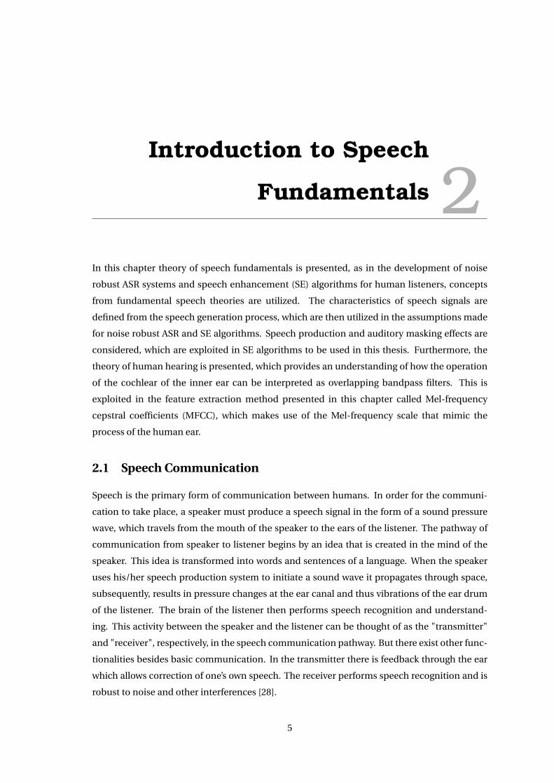
of SE and noise-robust ASR algorithms. The speech waveform is a pressure wave which is
generated by movements of anatomical structures that make up the human speech production
system. In Figure 2.1, a cross-sectional view of the anatomy of speech production is shown. The
speech organs can be divided into three main groups: the lungs, the larynx and the vocal tract
[28].
Vocal tract
Larynx
LungsRib cage
Diaphragm
Figure 2.1: The anatomy of speech production [28].
The purpose of lungs is the inhalation and exhalation of air. When inhaling air, the chest cavity
is enlarged, where the air pressure in the lungs is lowered. This causes the air to rush through
the vocal tract, down the trachea and into the lungs. When exhaling air, the volume of the chest
cavity is reduced, which increases air pressure within the lung. The increase in pressure causes
air to flow through the trachea into the larynx. The lungs then act as a "power supply" and
provide airflow to the larynx stage of the speech production process [16, 28].
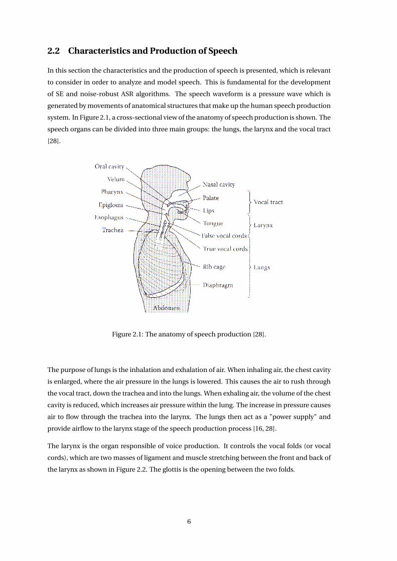
The larynx is the organ responsible of voice production. It controls the vocal folds (or vocal
cords), which are two masses of ligament and muscle stretching between the front and back of
the larynx as shown in Figure 2.2. The glottis is the opening between the two folds.
6
Thyroidcartilage \---,
Vocalfolds
Glottalslit
Arytenoidcartilage
(a) Larynx in the voicing state. (b) Larynx in the breathing state.
Figure 2.2: Sketches of the human larynx from a downward-looking view [28].
The vocal folds can assume three states: breathing, voiced and unvoiced. In the breathing
state, the glottis is wide open as shown in Figure 2.2b. The air from the lungs flows freely
through the glottis with no notable resistance from the vocal folds. In the voicing state, as the
production of a vowel (e.g. /aa/), the arytenoid cartilages move toward each other as shown in
Figure 2.2a. The tension of the folds increases and decreases, while the pressure at the glottis
increases and decreases, which makes the folds open and close periodically. The time duration
of one glottal cycle, which is the time between successive vocal openings, is known as the pitch
period and the reciprocal of the pitch period is known as the fundamental frequency. Thus the
periodically vibration of the vocal folds is responsible for "voiced" speech sounds. Unvoiced
sounds is generated when the vocal folds are in the unvoicing state. The state is similar to the
breathing state in that the vocal folds do not vibrate. The folds, however, are tenser and come
closer together, thus allowing the air stream to become turbulent as it flows through the glottis.
This air turbulence is called aspiration. Aspiration occurs in normal speech when producing
sounds like /h/ as in "house" or when whispering. Unvoiced sound include the majority of
consonants [16].
The vocal tract consists of the oral cavity and the nasal cavity. The input to the vocal tract is
the air flow wave coming via the vocal folds. The vocal tract acts a physical linear filter that
spectrally shapes the input wave to produce distinctly different sounds. The characteristics of
the filter (e.g. frequency response) change depending on the position of the articulators, i.e.
the shape of the oral cavity [16].
Characteristic of the speech signal can be defined from the speech generation process [16, 28,
37]:
• Speech signals are changing continuously and gradually, not abruptly. They are time
7
variant.
• The frequency content of a speech signal is changing across time. But the speech signal
can be divided into sound segments which have some common acoustic properties for a
short time interval. Therefore speech signals are referred to as being quasi-stationary.
• When producing voiced speech, air is exhaled out of the lungs through the trachea and
is interrupted periodically by the vibrating vocal cords. This means that voiced speech is
periodic in nature, where the frequency of the excitation provided by the vocal cords is
known as the fundamental frequency.
• At unvoiced regions, the speech signal has a stochastic spectral characteristic, where the
vocal cords do not vibrate and the excitation is provided by turbulent airflow through a
constriction in the vocal tract. This gives the time-domain representation of phonemes
(sound classes) a noisy characteristic.
• When producing speech and communicating to a listener, phrases or sentences are
constructed by choosing from a collection of finite mutually exclusive sounds. The basic
lingustic unit of speech is called phoneme. Many different factors, including for example,
gender, accents and coarticulatory effects, cause acoustic variations in the production of
a given "phoneme". Phonemes represents the way we understand sounds produced in
speech. Therefore, the phoneme represents a class of sound that has the same meaning.
These have to be distinguished from the actual sounds produced in speaking called
phones.
2.3 Speech Production Model
The vocal tract can be modelled as a linear filter that spectrally shapes the input wave to
produce different sounds, as described in Section 2.2. The characteristics of the vocal tract
have led to the development of an engineering model of speech production, as shown in Figure
2.3 [16]. This speech production model is considered, as it is utilized in the SE algorithm called
iterative Wiener filtering (IWF) [16] presented in Section 4.1.
8
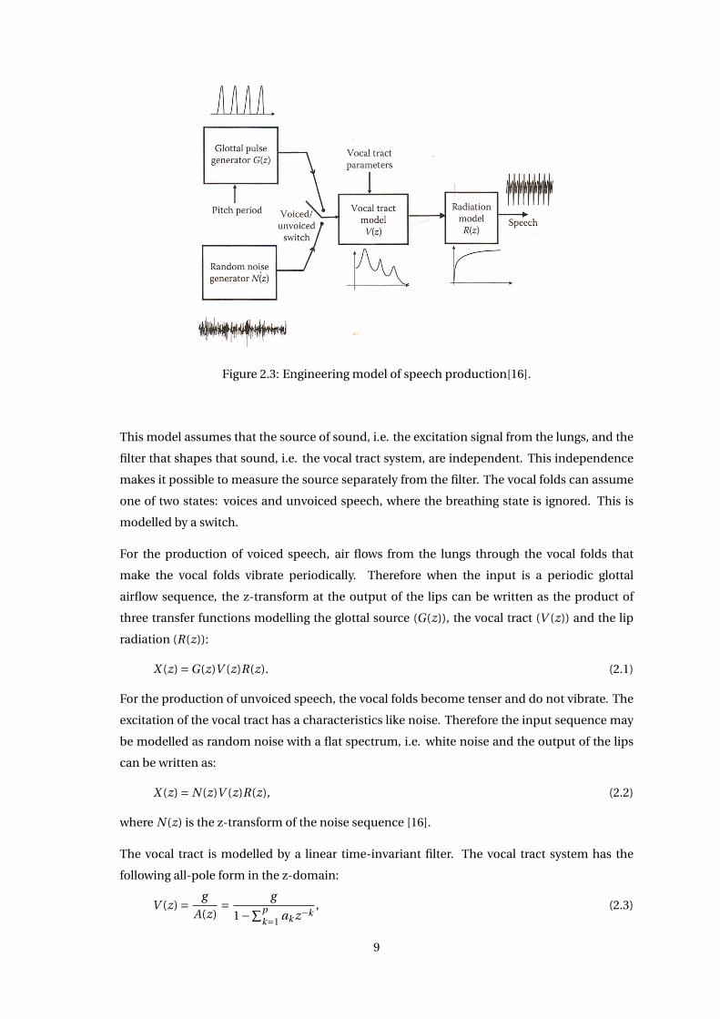
Figure 2.3: Engineering model of speech production[16].
This model assumes that the source of sound, i.e. the excitation signal from the lungs, and the
filter that shapes that sound, i.e. the vocal tract system, are independent. This independence
makes it possible to measure the source separately from the filter. The vocal folds can assume
one of two states: voices and unvoiced speech, where the breathing state is ignored. This is
modelled by a switch.
For the production of voiced speech, air flows from the lungs through the vocal folds that
make the vocal folds vibrate periodically. Therefore when the input is a periodic glottal
airflow sequence, the z-transform at the output of the lips can be written as the product of
three transfer functions modelling the glottal source (G(z)), the vocal tract (V (z)) and the lip
radiation (R(z)):
X (z) =G(z)V (z)R(z). (2.1)
For the production of unvoiced speech, the vocal folds become tenser and do not vibrate. The
excitation of the vocal tract has a characteristics like noise. Therefore the input sequence may
be modelled as random noise with a flat spectrum, i.e. white noise and the output of the lips
can be written as:
X (z) = N (z)V (z)R(z), (2.2)
where N (z) is the z-transform of the noise sequence [16].
The vocal tract is modelled by a linear time-invariant filter. The vocal tract system has the
following all-pole form in the z-domain:
V (z) = g
A(z)= g
1−∑pk=1 ak z−k
, (2.3)
9
where g is the gain of the system, {ak } are the all-pole coefficients and p is the number of
coefficients. The output of the vocal tract filter is fed to the sound radiation filter, that model
the effect of sound radiation at the lips. A filter of the following form is typically used as the
sound radiation filter:
R(z) = 1− z−1. (2.4)
This sound radiation block introduces about a 6 dB/octave high-pass boost. The output of the
model is the speech signal, which is generally observable [16].
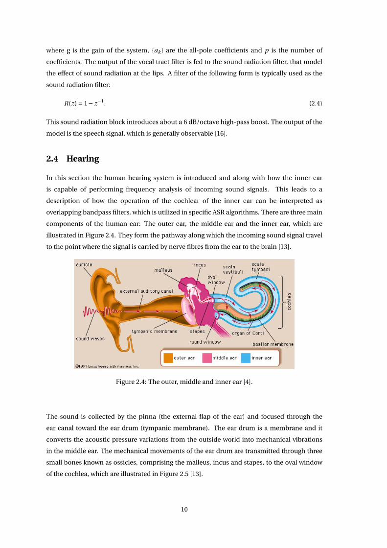
2.4 Hearing
In this section the human hearing system is introduced and along with how the inner ear
is capable of performing frequency analysis of incoming sound signals. This leads to a
description of how the operation of the cochlear of the inner ear can be interpreted as
overlapping bandpass filters, which is utilized in specific ASR algorithms. There are three main
components of the human ear: The outer ear, the middle ear and the inner ear, which are
illustrated in Figure 2.4. They form the pathway along which the incoming sound signal travel
to the point where the signal is carried by nerve fibres from the ear to the brain [13].
Figure 2.4: The outer, middle and inner ear [4].
The sound is collected by the pinna (the external flap of the ear) and focused through the
ear canal toward the ear drum (tympanic membrane). The ear drum is a membrane and it
converts the acoustic pressure variations from the outside world into mechanical vibrations
in the middle ear. The mechanical movements of the ear drum are transmitted through three
small bones known as ossicles, comprising the malleus, incus and stapes, to the oval window
of the cochlea, which are illustrated in Figure 2.5 [13].
10
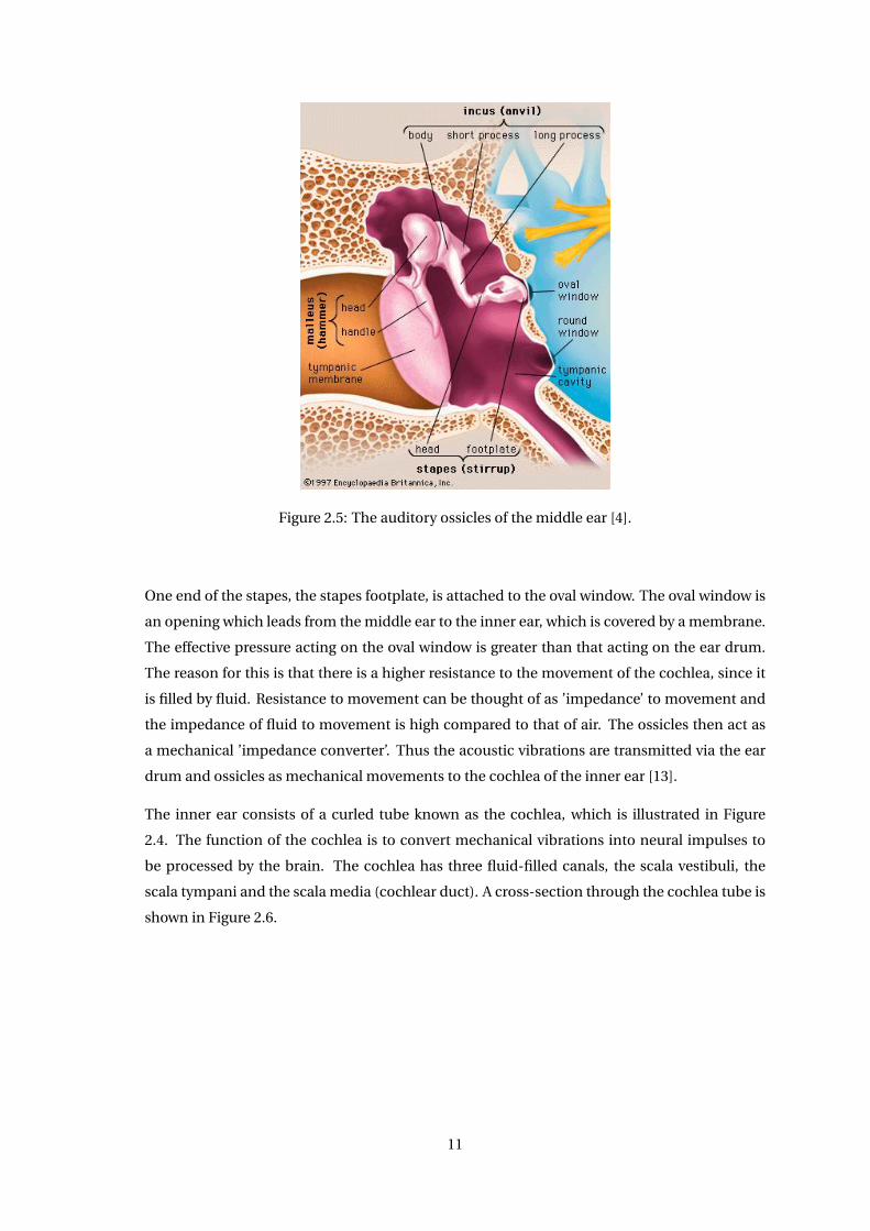
Figure 2.5: The auditory ossicles of the middle ear [4].
One end of the stapes, the stapes footplate, is attached to the oval window. The oval window is
an opening which leads from the middle ear to the inner ear, which is covered by a membrane.
The effective pressure acting on the oval window is greater than that acting on the ear drum.
The reason for this is that there is a higher resistance to the movement of the cochlea, since it
is filled by fluid. Resistance to movement can be thought of as ’impedance’ to movement and
the impedance of fluid to movement is high compared to that of air. The ossicles then act as
a mechanical ’impedance converter’. Thus the acoustic vibrations are transmitted via the ear
drum and ossicles as mechanical movements to the cochlea of the inner ear [13].
The inner ear consists of a curled tube known as the cochlea, which is illustrated in Figure
2.4. The function of the cochlea is to convert mechanical vibrations into neural impulses to
be processed by the brain. The cochlea has three fluid-filled canals, the scala vestibuli, the
scala tympani and the scala media (cochlear duct). A cross-section through the cochlea tube is
shown in Figure 2.6.
11
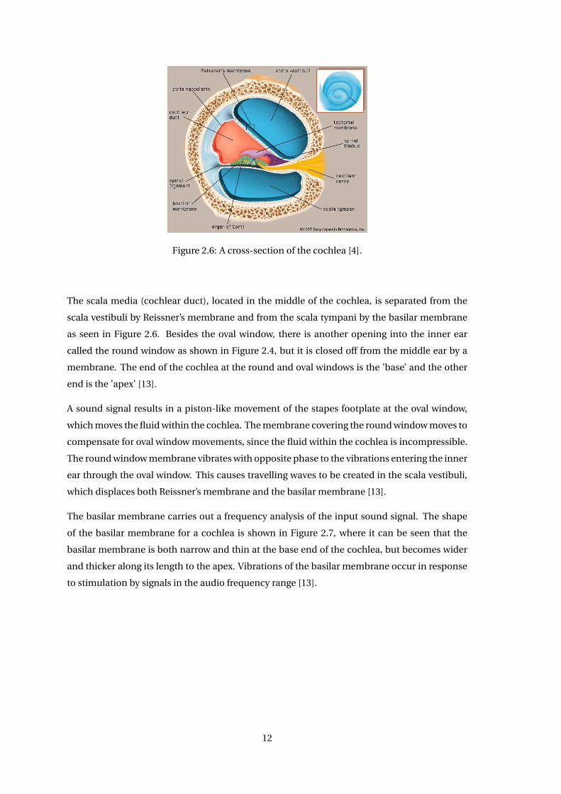
Figure 2.6: A cross-section of the cochlea [4].
The scala media (cochlear duct), located in the middle of the cochlea, is separated from the
scala vestibuli by Reissner’s membrane and from the scala tympani by the basilar membrane
as seen in Figure 2.6. Besides the oval window, there is another opening into the inner ear
called the round window as shown in Figure 2.4, but it is closed off from the middle ear by a
membrane. The end of the cochlea at the round and oval windows is the ’base’ and the other
end is the ’apex’ [13].
A sound signal results in a piston-like movement of the stapes footplate at the oval window,
which moves the fluid within the cochlea. The membrane covering the round window moves to
compensate for oval window movements, since the fluid within the cochlea is incompressible.
The round window membrane vibrates with opposite phase to the vibrations entering the inner
ear through the oval window. This causes travelling waves to be created in the scala vestibuli,
which displaces both Reissner’s membrane and the basilar membrane [13].
The basilar membrane carries out a frequency analysis of the input sound signal. The shape
of the basilar membrane for a cochlea is shown in Figure 2.7, where it can be seen that the
basilar membrane is both narrow and thin at the base end of the cochlea, but becomes wider
and thicker along its length to the apex. Vibrations of the basilar membrane occur in response
to stimulation by signals in the audio frequency range [13].
12
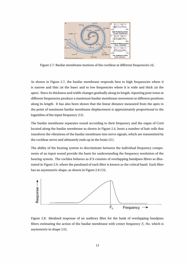
Figure 2.7: Basilar membrane motions of the cochlear at different frequencies [4].
As shown in Figure 2.7, the basilar membrane responds best to high frequencies where it
is narrow and thin (at the base) and to low frequencies where it is wide and thick (at the
apex). Since its thickness and width changes gradually along its length, inputting pure tones at
different frequencies produce a maximum basilar membrane movement at different positions
along its length. It has also been shown that the linear distance measured from the apex to
the point of maximum basilar membrane displacement is approximately proportional to the
logarithm of the input frequency [13].
The basilar membrane separates sound according to their frequency and the organ of Corti
located along the basilar membrane as shown in Figure 2.4, hosts a number of hair cells that
transform the vibrations of the basilar membrane into nerve signals, which are transmitted by
the cochlear nerve and ultimately ends up in the brain [21].
The ability of the hearing system to discriminate between the individual frequency compo-
nents of an input sound provide the basis for understanding the frequency resolution of the
hearing system. The cochlea behaves as if it consists of overlapping bandpass filters as illus-
trated in Figure 2.9, where the passband of each filter is known as the critical band. Each filter
has an asymmetric shape, as shown in Figure 2.8 [13].
Figure 2.8: Idealised response of an auditory filter for the bank of overlapping bandpass
filters estimating the action of the basilar membrane with center frequency Fc Hz, which is
asymmetric in shape [13].
13
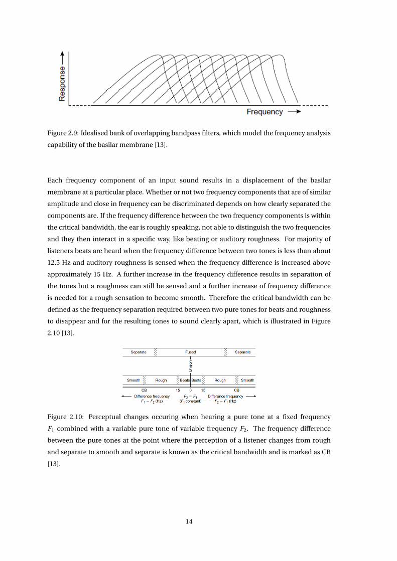
Figure 2.9: Idealised bank of overlapping bandpass filters, which model the frequency analysis
capability of the basilar membrane [13].
Each frequency component of an input sound results in a displacement of the basilar
membrane at a particular place. Whether or not two frequency components that are of similar
amplitude and close in frequency can be discriminated depends on how clearly separated the
components are. If the frequency difference between the two frequency components is within
the critical bandwidth, the ear is roughly speaking, not able to distinguish the two frequencies
and they then interact in a specific way, like beating or auditory roughness. For majority of
listeners beats are heard when the frequency difference between two tones is less than about
12.5 Hz and auditory roughness is sensed when the frequency difference is increased above
approximately 15 Hz. A further increase in the frequency difference results in separation of
the tones but a roughness can still be sensed and a further increase of frequency difference
is needed for a rough sensation to become smooth. Therefore the critical bandwidth can be
defined as the frequency separation required between two pure tones for beats and roughness
to disappear and for the resulting tones to sound clearly apart, which is illustrated in Figure
2.10 [13].
Figure 2.10: Perceptual changes occuring when hearing a pure tone at a fixed frequency
F1 combined with a variable pure tone of variable frequency F2. The frequency difference
between the pure tones at the point where the perception of a listener changes from rough
and separate to smooth and separate is known as the critical bandwidth and is marked as CB
[13].
14
2.5 Auditory Masking
The scenario where one sound is made inaudible in the presence of other sounds is referred to
as masking. Auditory masking is considered as it is utilized in the SE algorithms considered in
this thesis called audible noise suppression (ANS) [16] and the short-time spectral amplitude
(STSA) estimator based on the weighted euclidean (WE) distortion measure [16], which are
presented in Section 4.2 and Subsection 4.3.1, respectively. The sound source which causes
the masking is known as the masker and the sound source which is masked is known as the
maskee. There are two types of masking principles:
• Simultaneous masking: When two sound events, masker and maskee, occur at the same
time.
• Non-simultaneous masking: A situation where the masker and maskee is out of
synchrony and do not occur at the same time.
Only simultaneous masking is relevant in this thesis, where speech signals with additive noise
is considered. The unmasked threshold is the smallest level of the maskee which can be
perceived without a masking signal is present. The masked threshold is the lowest level of
the maskee necessary to be just audible in the presence of a masker. The amount of masking is
the difference in dB between the masked and the unmasked threshold [8, 13].
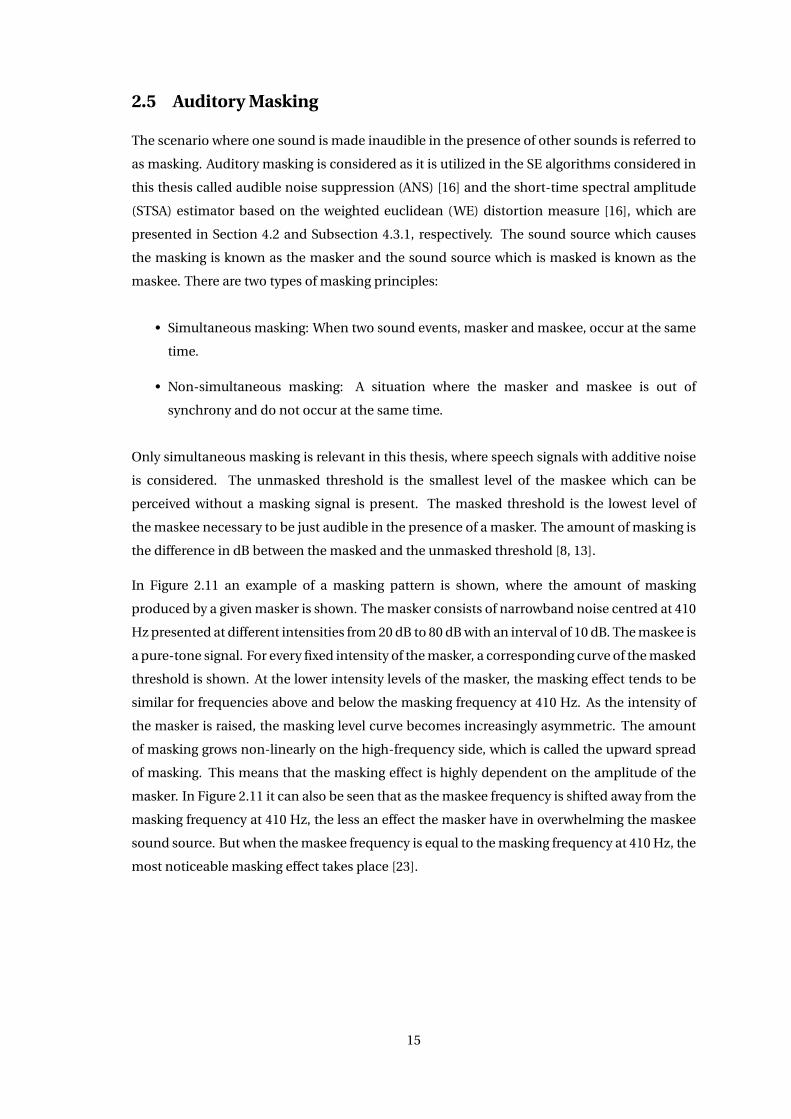
In Figure 2.11 an example of a masking pattern is shown, where the amount of masking
produced by a given masker is shown. The masker consists of narrowband noise centred at 410
Hz presented at different intensities from 20 dB to 80 dB with an interval of 10 dB. The maskee is
a pure-tone signal. For every fixed intensity of the masker, a corresponding curve of the masked
threshold is shown. At the lower intensity levels of the masker, the masking effect tends to be
similar for frequencies above and below the masking frequency at 410 Hz. As the intensity of
the masker is raised, the masking level curve becomes increasingly asymmetric. The amount
of masking grows non-linearly on the high-frequency side, which is called the upward spread
of masking. This means that the masking effect is highly dependent on the amplitude of the
masker. In Figure 2.11 it can also be seen that as the maskee frequency is shifted away from the
masking frequency at 410 Hz, the less an effect the masker have in overwhelming the maskee
sound source. But when the maskee frequency is equal to the masking frequency at 410 Hz, the
most noticeable masking effect takes place [23].
15
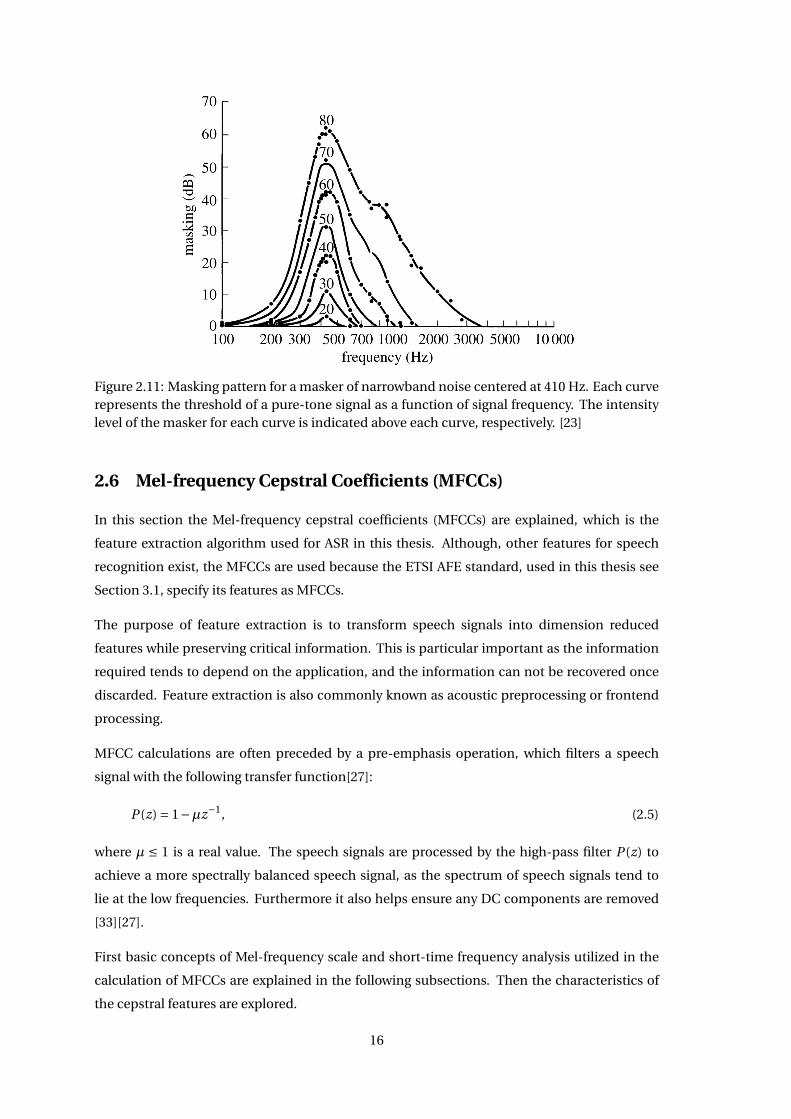
Figure 2.11: Masking pattern for a masker of narrowband noise centered at 410 Hz. Each curverepresents the threshold of a pure-tone signal as a function of signal frequency. The intensitylevel of the masker for each curve is indicated above each curve, respectively. [23]
2.6 Mel-frequency Cepstral Coefficients (MFCCs)
In this section the Mel-frequency cepstral coefficients (MFCCs) are explained, which is the
feature extraction algorithm used for ASR in this thesis. Although, other features for speech
recognition exist, the MFCCs are used because the ETSI AFE standard, used in this thesis see
Section 3.1, specify its features as MFCCs.
The purpose of feature extraction is to transform speech signals into dimension reduced
features while preserving critical information. This is particular important as the information
required tends to depend on the application, and the information can not be recovered once
discarded. Feature extraction is also commonly known as acoustic preprocessing or frontend
processing.
MFCC calculations are often preceded by a pre-emphasis operation, which filters a speech
signal with the following transfer function[27]:
P (z) = 1−µz−1, (2.5)
where µ ≤ 1 is a real value. The speech signals are processed by the high-pass filter P (z) to
achieve a more spectrally balanced speech signal, as the spectrum of speech signals tend to
lie at the low frequencies. Furthermore it also helps ensure any DC components are removed
[33][27].
First basic concepts of Mel-frequency scale and short-time frequency analysis utilized in the
calculation of MFCCs are explained in the following subsections. Then the characteristics of
the cepstral features are explored.
16
2.6.1 Mel-frequency Scale
Due to effectiveness of the human auditory system in perceiving and recognizing human
speech, feature extraction techniques based on the characteristics of the human auditory
system have been shown to provide excellent performance for ASR [38].
The Mel-frequency scale models the human ear in regard to the non-linear properties of pitch
perception. The scale was proposed in 1937 by Stevens, Volkmann and Newman [31], based on
experiments where test subjects were asked to adjust the frequency of a tone until they judged
it to be half of a fixed tone. The name is meant to symbolise that the scale is based on pitch
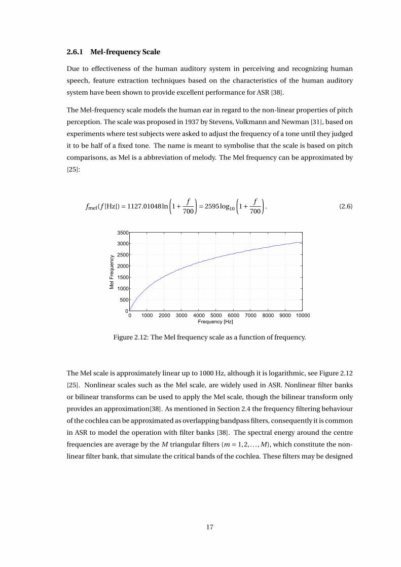
comparisons, as Mel is a abbreviation of melody. The Mel frequency can be approximated by
[25]:
fmel( f [Hz]) = 1127.01048ln
(1+ f
700
)= 2595log10
(1+ f
700
). (2.6)
0 1000 2000 3000 4000 5000 6000 7000 8000 9000 100000
500
1000
1500
2000
2500
3000
3500
Frequency [Hz]
Mel
Fre
quen
cy
Figure 2.12: The Mel frequency scale as a function of frequency.
The Mel scale is approximately linear up to 1000 Hz, although it is logarithmic, see Figure 2.12
[25]. Nonlinear scales such as the Mel scale, are widely used in ASR. Nonlinear filter banks
or bilinear transforms can be used to apply the Mel scale, though the bilinear transform only
provides an approximation[38]. As mentioned in Section 2.4 the frequency filtering behaviour
of the cochlea can be approximated as overlapping bandpass filters, consequently it is common
in ASR to model the operation with filter banks [38]. The spectral energy around the centre
frequencies are average by the M triangular filters (m = 1,2, . . . , M), which constitute the non-
linear filter bank, that simulate the critical bands of the cochlea. These filters may be designed
17
by[38]:
Hm[k] =
0, k < f [m −1]2(k− f [m−1])
( f [m+1]− f [m−1])( f [m]− f [m−1]) , f [m −1] ≤ k ≤ f [m]2( f [m+1]−k)
( f [m+1]− f [m−1])( f [m+1]− f [m]) , f [m] ≤ k ≤ f [m +1]
0, k > f [m +1]
, (2.7)
where f is defined as:
f [m] = N
fsamplingf −1
mel( flowest +mflowest − fhighest
M +1). (2.8)
flowest and fhighest are the lowest and highest frequencies of the filter bank, respectively, and N
are the number of bins in the linear frequency domain. The triangular filters are designed such
that the half way point between center frequencies is the 3 dB point, i.e. the point where its
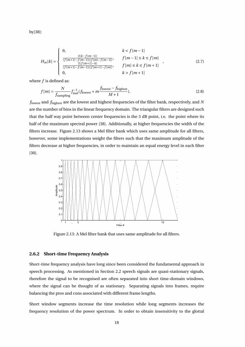
half of the maximum spectral power [38]. Additionally, at higher frequencies the width of the
filters increase. Figure 2.13 shows a Mel filter bank which uses same amplitude for all filters,
however, some implementations weight the filters such that the maximum amplitude of the
filters decrease at higher frequencies, in order to maintain an equal energy level in each filter
[30].
1 ... 5 ... 150
0.1
0.2
0.3
0.4
0.5
0.6
0.7
0.8
0.9
1
Am
plitu
de
Filter #
Figure 2.13: A Mel filter bank that uses same amplitude for all filters.
2.6.2 Short-time Frequency Analysis
Short-time frequency analysis have long since been considered the fundamental approach in
speech processing. As mentioned in Section 2.2 speech signals are quasi-stationary signals,
therefore the signal to be recognised are often separated into short time-domain windows,
where the signal can be thought of as stationary. Separating signals into frames, require
balancing the pros and cons associated with different frame lengths.
Short window segments increase the time resolution while long segments increases the
frequency resolution of the power spectrum. In order to obtain insensitivity to the glottal
18
cycle relative to the position of the frame, an adequate an frame length is necessary[38]. Both
the degree of smoothing of the temporal variations during unvoiced speech and the degree of
blurring for rapid event (e.g. release of stop consonants) are determined by the frame length.
Consequently the frame length should ideally depend on the speed with which the vocal tract
changes shape. The values assigned to frame length and the frame shift ensures the frame
overlap each other, with typical values being between 16-32ms and 5-15ms, respectively [38].
The speech signal is segmented into frames via a windowing function. The shape of the
window function influences the characteristics of the frequency domain of the frame, where
the frequency resolution is in particular affected by this. It is desired to avoid abrupt edges in
the windows, which leads to large sidelobes in the frequency domain [38], as the spectrum of
the frame is convolved together with the Fourier transform of the window function. Therefore
there arises a leakage of the energy from a given frequency into adjacent regions. This is what
is normally referred to as spectral leakage, the size of which is proportional to the magnitude
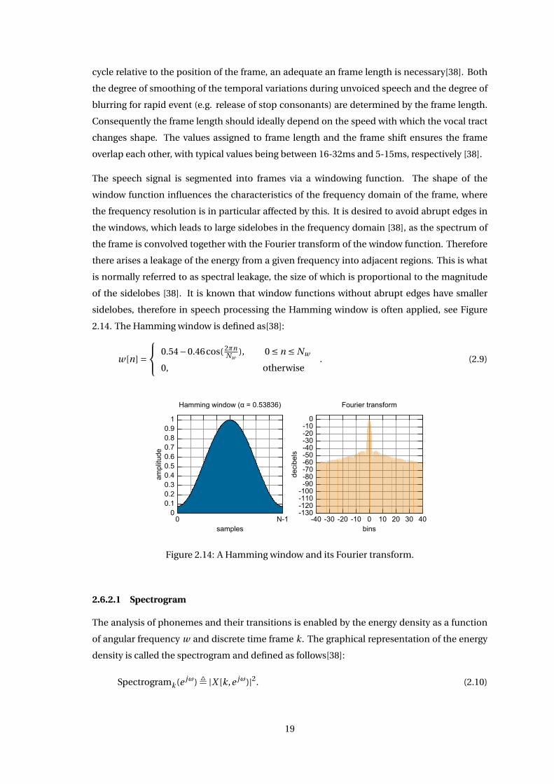
of the sidelobes [38]. It is known that window functions without abrupt edges have smaller
sidelobes, therefore in speech processing the Hamming window is often applied, see Figure
2.14. The Hamming window is defined as[38]:
w[n] = 0.54−0.46cos( 2πn
Nw), 0 ≤ n ≤ Nw
0, otherwise. (2.9)
00.10.20.30.40.50.60.70.80.9
1
0 N-1
ampl
itude
samples
Hamming)window)(α)=)0.53836)
-130-120-110-100
-90-80-70-60-50-40-30-20-10
0
-40 -30 -20 -10 0 10 20 30 40
deci
bels
bins
Fourier)transform
Figure 2.14: A Hamming window and its Fourier transform.
2.6.2.1 Spectrogram
The analysis of phonemes and their transitions is enabled by the energy density as a function
of angular frequency w and discrete time frame k. The graphical representation of the energy
density is called the spectrogram and defined as follows[38]:
Spectrogramk (e jω), |X [k,e jω)|2. (2.10)
19
X [k,e jω) is the short-time Fourier transform (STFT) given by:
X [k,e jω),∞∑
m=−∞x[n +m]w[m]e− jωm , (2.11)
where k is discrete and ω is continuous, w[m] is a window function e.g. a Hamming or
Gaussian window function, which is used to break the signal into frames. Each frame is then
Fourier transformed. In speech applications spectrograms tends to utilize the logarithmic
frequency scale because human speech has a large dynamic range[38]:
Logarithmic Spectrogramk (e jω) = 20log10 |X [k,e jω)|. (2.12)
Depending on whether the duration of the window used, is short (less than one pitch
period) or long (≥ two pitch periods), the utilized spectrogram is differentiated between wide-
band or narrow-band, respectively [38]. The use of wide-band spectrogram results in good
time resolution, but the harmonic structure is smeared. In comparison, the narrow-band
spectrogram provides better frequency resolution but poorer time resolution. In addition,
during segments containing voiced speech the harmonics of the pitch can be observed as
horizontal striations due to the increased frequency resolution [38].
2.6.3 Definition and Characteristics of Cepstral Sequences
Although originally intended for differentiation of underground echoes [38], cepstral features
have been used in ASR for more than 30 years and is today widely used in a range for of different
speech applications. The names stem from the inventors who realized that the operations
they utilize in the transform domain, are typical exclusively used in the time domain. Hence,
the name cepstrum was chosen by reversing the first letters in spectrum[38]. The complex
cepstrum z-transform is defined as:
X (z), log X (z), (2.13)
where X (z) is the z-transform of a stable sequence x(n) (n is the discrete time index), X (z) is
the z-transform of the complex cepstrum and log(·) is a complex-valued logarithm, hence the
name complex cepstrum. This leads to the following definition for the complex cepstrum[38]:
x[n] = 1
2π
∫ π
−πlog X (e jω)e jωndω, (2.14)
which is the inverse Fourier transform of log X (e jω), the real cepstrum is then defined as:
cx [n],1
2π
∫ π
−πlog |X (e jω)|e jωndω. (2.15)
The real cepstrum cx [n] is the inverse transform of the real part of X (e jω). Characteristics of
the cepstral sequence is investigated using the time-series cepstral representation h[n] of a
transfer system of a linear time-invariant system [38]:
h[n] =
log |K |, n = 0
−∑Mim=1
cnmn +∑Ni
m=1d n
mn , n > 0
−∑Mom=1
a−nmn −∑No
m=1b−n
mn , n < 0
, (2.16)
20
where |am |, |bm |,|cm |,|dm | < 1, Mi and Ni are the number of zeroes and poles inside the unit
circle, respectively. Mo and No are the number of zeroes and poles outside the unit circle, and
K is a real constant.
It can be shown that the cepstrals coefficients are a casual sequence of the system if it is a
minimum phase system (i.e. both the transfer function of the system and its inverse are stable
and casual), meaning that h[n] = 0 ∀ n < 0. In addition the cepstral coefficient h(n) decay
at a rate of at least 1/n meaning most information about the spectral shape of the transfer
system is contained with the lower order coefficients. It is possible to derive a second cepstral
sequence xmin[n] for the minimum phase system, where the cepstra of xmin[n] and x[n] have
the different phase but the same magnitude. An expression for xmi n[0] can then be derived
as[38]:
xmin[n] =
0, n < 0
x[0], n = 0
2x[n], n > 0
. (2.17)
Especially xmi n[0] and xmi n[1] of the lower order cepstral coefficient can be given intuitive
meaning. The average power of the input signal can be observed in xmi n[0], though for ASR
purposes more reliable power measures are typical utilized. xmi n[1] is on the other hand a
measure of how the spectral energy is distributed between high and low frequencies [38]. The
sign of xmi n[1] provides information about where the spectral energy is concentrated, positive
and negative values indicate energy concentration at low and high frequencies, respectively
[38].
Increasing levels of spectral details can be found in the higher order cepstral coefficients.
It can be shown that an infinite number of cepstral coefficients is produced by an finite
input sequence, however, to archive accurately ASR results a finite number of coefficients is
sufficient[38]. Depending on the sampling rate, only the first 12-20 coefficients are typically
used. This occurs because lower order coefficients contribute more than higher orders to class
separation [38].
Discarding the higher orders of the cepstral coefficients provide an additional benefit due to
another characteristic of the cepstral sequence. By removing the higher order coefficients
from a sequence of cepstral coefficients it is possible to remove the periodic excitation p[n]
occurring due to the vocal cords. If it is assumed that the sequence x[n] is given by convolution:
x[n] = h[n]∗p[n], (2.18)
where h[n] is the impulse response of a linear time-invariant system and p[n] is the periodic
excitation with an period T0 of the system. Removing p[n] from the speech signal x[n] is
advantageous as the goal is to extract a representation of h[n] from x[n]. From this the
21
following expression for the complex cepstrum can then be derived [38]:
x[n] = h[n]+ p[n], (2.19)
meaning that if two sequences are convolved in the time domain, then their complex cepstra
are simply added together. Combining this with Equation 2.17, the cepstral sequence for
minimum phase system can then be expressed as:
xmin[n] = hmin[n]+ pmin[n]. (2.20)
It has been proven [38] that when p[n] is an periodic excitation with a period T0, then p[0] = 0
and p[n] is periodic with period of N0 = T0/Ts samples [38], where Ts is an sampling interval.
Consequently, p[n] is only nonzero at p[kN0]. Meaning that the liftering (the name comes from
reversing the first four letters of filtering) operation can be utilized to recover hmin[n] [38]:
hmin[n] ≈ xmin[n]ω[n], (2.21)
where
ω[n] = 1, ∀0 ≤ n < N0,
0, otherwise.(2.22)
If h[n] then is the impulse response of the vocal tract of a speaker and p[n] the periodic
excitation produced by the vocal cords during voiced speech, Equation 2.21 shows how the
cepstral domain can remove the periodic excitation resulting from the vocal cords, by simply
removing higher order cepstral coefficients, so that spectral envelope made by the shape of the
vocal tract can be found [38].
2.6.4 Calculating Cepstral Coefficients
In ASR acoustic features are typical produced from the minimum phase equivalent xmi n[n]
of the cepstral sequence. These features can be found by calculating an intermediate value
cx [n] (2.15) using the inverse discrete Fourier transform (DFT), which can be used to find
xmi n[n][38]:
xmin[n] =
0, n < 0
cx [0], n = 0
2cx [n], n > 0
. (2.23)
Another option is to use the type 2 discrete cosine transform (DCT), to apply the inverse DCT
to log-power spectral density log |X (e jω)|:
xmin[n] =M−1∑m=0
log |X (e jωm )|T (2)n,m , (2.24)
where T (2)n,m is a component of the type 2 DCT. The calculation of the MPCCs is summarized
in Figure 2.15. First the pre-emphasis spectrally balance the signal using a high-pass filter.
22
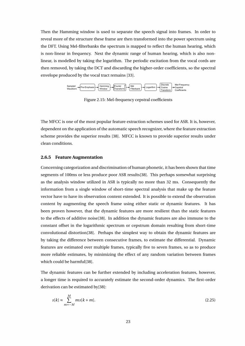
Then the Hamming window is used to separate the speech signal into frames. In order to
reveal more of the structure these frame are then transformed into the power spectrum using
the DFT. Using Mel-filterbanks the spectrum is mapped to reflect the human hearing, which
is non-linear in frequency. Next the dynamic range of human hearing, which is also non-
linear, is modelled by taking the logarithm. The periodic excitation from the vocal cords are
then removed, by taking the DCT and discarding the higher-order coefficients, so the spectral
envelope produced by the vocal tract remains [33].
SampledWaveform
Mel-FrequencyCepstralbCoefficients
Pre-Emphasis HammingbWindow
MelFilterbank
LogarithmDiscretebCosineTransform
FourierbbbbbbTransform
2
Figure 2.15: Mel-frequency cepstral coefficients
The MFCC is one of the most popular feature extraction schemes used for ASR. It is, however,
dependent on the application of the automatic speech recognizer, where the feature extraction
scheme provides the superior results [38]. MFCC is known to provide superior results under
clean conditions.
2.6.5 Feature Augmentation
Concerning categorization and discrimination of human phonetic, it has been shown that time
segments of 100ms or less produce poor ASR results[38]. This perhaps somewhat surprising
as the analysis window utilized in ASR is typically no more than 32 ms. Consequently the
information from a single window of short-time spectral analysis that make up the feature
vector have to have its observation content extended. It is possible to extend the observation
content by augmenting the speech frame using either static or dynamic features. It has
been proven however, that the dynamic features are more resilient than the static features
to the effects of additive noise[38]. In addition the dynamic features are also immune to the
constant offset in the logarithmic spectrum or cepstrum domain resulting from short-time
convolutional distortion[38]. Perhaps the simplest way to obtain the dynamic features are
by taking the difference between consecutive frames, to estimate the differential. Dynamic
features are estimated over multiple frames, typically five to seven frames, so as to produce
more reliable estimates, by minimizing the effect of any random variation between frames
which could be harmful[38].
The dynamic features can be further extended by including acceleration features, however,
a longer time is required to accurately estimate the second-order dynamics. The first-order
derivation can be estimated by[38]:
s[k] ≈M∑
m=−Mms[k +m]. (2.25)
23
Higher order derivations can be found by reapplying the linear phase filter in Equation 2.25
consecutively to output from the previous order. The first and second order derivations is
referred to as the Delta and Delta-Delta coefficients, respectively.
24
Automatic Speech
Recognition 3This chapter presents the feature extraction method and the machine learning algorithm,
which are used to generate the ASR results within this thesis. The speech database to be
used for training acoustic models and for recognition experiments is described along with the
performance evaluation measures.
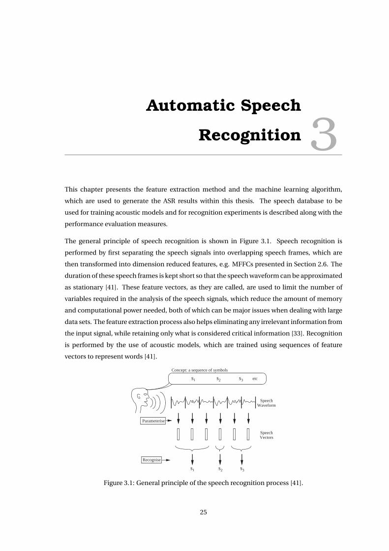
The general principle of speech recognition is shown in Figure 3.1. Speech recognition is
performed by first separating the speech signals into overlapping speech frames, which are
then transformed into dimension reduced features, e.g. MFFCs presented in Section 2.6. The
duration of these speech frames is kept short so that the speech waveform can be approximated
as stationary [41]. These feature vectors, as they are called, are used to limit the number of
variables required in the analysis of the speech signals, which reduce the amount of memory
and computational power needed, both of which can be major issues when dealing with large
data sets. The feature extraction process also helps eliminating any irrelevant information from
the input signal, while retaining only what is considered critical information [33]. Recognition
is performed by the use of acoustic models, which are trained using sequences of feature
vectors to represent words [41].
s1 s2 s3 etc
s1 s2 s3
SpeechWaveform
SpeechVectors
Concept: a sequence of symbols
Parameterise
Recognise
Figure 3.1: General principle of the speech recognition process [41].
25
In this thesis the ASR results are produced by the use of the advanced frontend (AFE) feature
extraction algorithm applied on the Aurora-2 database. In addition the Hidden Markov Model
Toolkit (HTK) is used to model speech and recognize speech. It has been chosen to use these
methods, as they have been used in [14] which raises the issue of applying an algorithm from
one field to the other. Furthermore, [12] intended to establish a baseline, using these methods,
to ease comparison of ASR performance. This make these methods suitable choices for this
thesis.
3.1 ETSI Advanced Front-End
The advanced frontend (AFE) is one of four standards developed by the European Telecommu-
nications Standards Institute (ETSI) that specify feature extraction and compression algorithms
for distributed speech recognition (DSR) [7]. DSR is one of three architectures used in ASR on
mobile devices, where the two other architectures are network speech recognition (NSR) and
embedded speech recognition (ESR)[33].
The ESR architechture is characterised by doing all the processing on the terminal site. The
NSR architecture is, however, characterised by transmitting an encoded speech signal from the
terminal to a server which decodes the speech signal and then performs feature extraction and
recognition. In DSR, feature extraction is performed by the terminal device, the features are
then transmitted to the server [27].
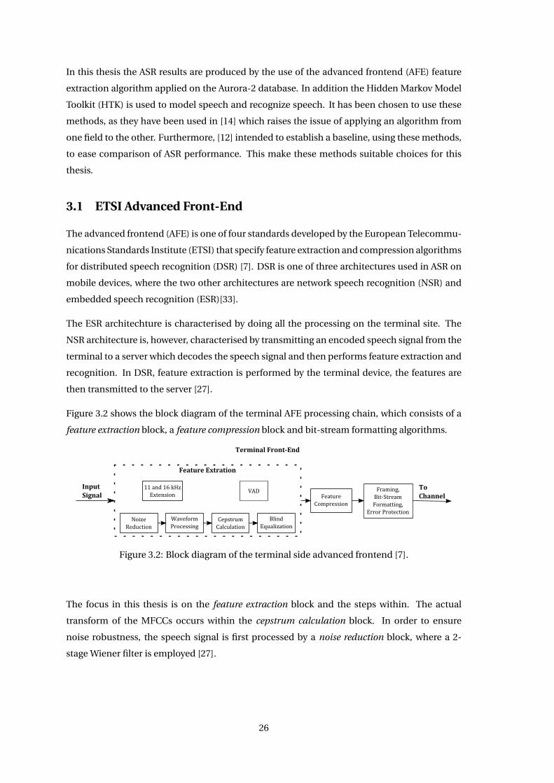
Figure 3.2 shows the block diagram of the terminal AFE processing chain, which consists of a
feature extraction block, a feature compression block and bit-stream formatting algorithms.
ToChannel
TerminalFront-End
FeatureCompression
Framing,Bit-StreamFormatting,
ErrorProtection
InputSignal
FeatureExtration
CepstrumCalculation
NoizeReduction
WaveformProcessing
BlindEqualization
11and16kHzExtension
VAD
Figure 3.2: Block diagram of the terminal side advanced frontend [7].
The focus in this thesis is on the feature extraction block and the steps within. The actual
transform of the MFCCs occurs within the cepstrum calculation block. In order to ensure
noise robustness, the speech signal is first processed by a noise reduction block, where a 2-
stage Wiener filter is employed [27].
26
3.1.1 Feature Extraction
In order to enable classification it is necessary to transform the input data into a suitable form
of MFCCs feature vectors. In addition to cepstrum calculation the feature extraction block
includes a number of sub-blocks, that perform preprocessing and postprocessing. The input
to the feature extraction block is fed to the noise reduction block, which uses Wiener filter
techniques. This is followed by waveform processing which attempts to maximise the signal-
to-noise ratio (SNR) using a time-domain approach, as opposed to the frequency-domain
approach used by the Wiener filters. The final stage after cepstrum calculation is the blind
equalization block which equalizes the cepstral coefficients according to a least mean square
filtering approach.
As standard the feature extraction block requires the speech signal to have a sampling rate of
8 kHz, which stems from the speech database used. Although, there are extensions available
allowing for 11 kHz and 16 kHz sampling rates. In this section the functionality of the each
block is presented.
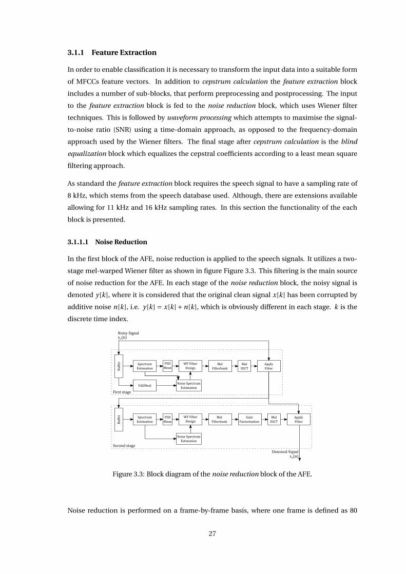
3.1.1.1 Noise Reduction
In the first block of the AFE, noise reduction is applied to the speech signals. It utilizes a two-
stage mel-warped Wiener filter as shown in figure Figure 3.3. This filtering is the main source
of noise reduction for the AFE. In each stage of the noise reduction block, the noisy signal is
denoted y[k], where it is considered that the original clean signal x[k] has been corrupted by
additive noise n[k], i.e. y[k] = x[k]+n[k], which is obviously different in each stage. k is the
discrete time index.
Buffer
Buffer
GainFactorization
MelFilterbank
SpectrumEstimation
MelIDCT
ApplyFilter
WFFilterDesign
NoiseSpectrumEstimation
ApplyFilter
MelFilterbank
WFFilterDesign
NoiseSpectrumEstimation
VADNest
SpectrumEstimation
MelIDCT
Firststage
Secondstage
PSDMean
PSDMean
Denoised Signalsof(n)
NoisySignalsin(n)
Figure 3.3: Block diagram of the noise reduction block of the AFE.
Noise reduction is performed on a frame-by-frame basis, where one frame is defined as 80
27
samples [7]. Each of the two stages operates with a 4 frame buffer. The first stage performs the
initial denoising of the signal, which is further processed in the second stage using dynamic
noise reduction depending on signal-to-noise ratio (SNR) of the output from the first stage [7].
It is because of the inaccurate spectrum estimates used during the first stage that the second
stage is necessary. The purpose of the spectrum estimation block is to find an estimation of the
linear spectrum for each frame. The PSD mean block then smooths out this spectrum estimate
along the time dimension. The noise spectrum estimation block uses the silent segments where
only the noise signal n[k] is present (located using Voice Activity Detection (VAD) for noise
estimation (VADNest)) to find an estimate of the noise spectrum. Then the frequency domain
Wiener filter coefficients are found in the WF Filter design block using both the spectrum and
noise spectrum estimates for the current frame. The Mel filterbank block smooth the linear
Wiener filter coefficients along the frequency domain using a Mel filterbank, to obtain a Mel-
warped frequency domain Wiener filter. The gain factorization block in the second stage
adjusts the aggressiveness of the noise reduction on a frame-by-frame basis depending on
whether it is a speech or silent frame. From the Mel-warped Wiener filter, the corresponding
impulse response is found by applying the Mel IDCT (Mel-warped Inverse Discrete Cosine
Transform). The Apply Filter block then filter the input signal at each stage [27]. In the following
the operation of each block in the noise reduction block is expanded upon.
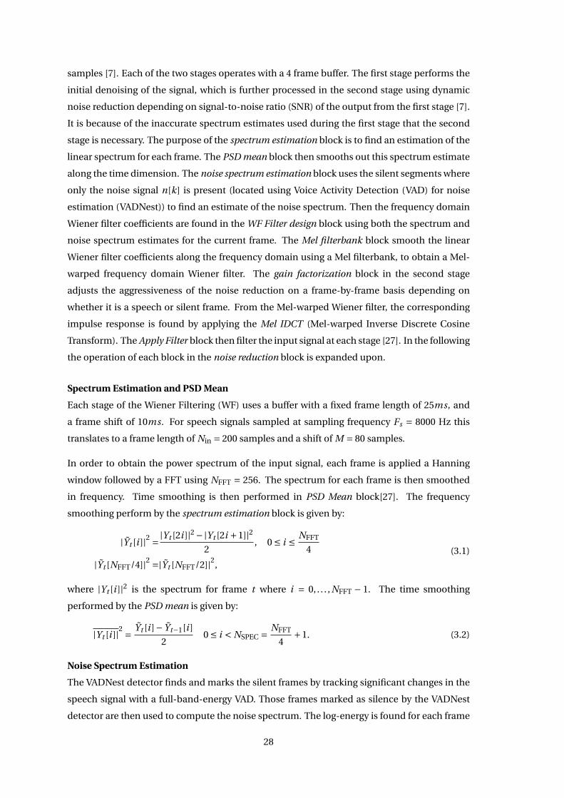
Spectrum Estimation and PSD Mean
Each stage of the Wiener Filtering (WF) uses a buffer with a fixed frame length of 25ms, and
a frame shift of 10ms. For speech signals sampled at sampling frequency Fs = 8000 Hz this
translates to a frame length of Nin = 200 samples and a shift of M = 80 samples.
In order to obtain the power spectrum of the input signal, each frame is applied a Hanning
window followed by a FFT using NFFT = 256. The spectrum for each frame is then smoothed
in frequency. Time smoothing is then performed in PSD Mean block[27]. The frequency
smoothing perform by the spectrum estimation block is given by:
|Yt [i ]|2 =|Yt [2i ]|2 −|Yt [2i +1]|22
, 0 ≤ i ≤ NFFT
4
|Yt [NFFT/4]|2 =|Yt [NFFT/2]|2,
(3.1)
where |Yt [i ]|2 is the spectrum for frame t where i = 0, . . . , NFFT − 1. The time smoothing
performed by the PSD mean is given by:
|Yt [i ]|2 = Yt [i ]− Yt−1[i ]
20 ≤ i < NSPEC = NFFT
4+1. (3.2)
Noise Spectrum Estimation
The VADNest detector finds and marks the silent frames by tracking significant changes in the
speech signal with a full-band-energy VAD. Those frames marked as silence by the VADNest
detector are then used to compute the noise spectrum. The log-energy is found for each frame
28
using the average background noise log-energy and the frame is then classified as speech or
silence based on the difference between the log-energy of the noisy signal and the log energy of
the background noise [27]. This decision is based on a fixed threshold. During silent frames the
noise spectrum estimation block finds estimates of the noise Nt [ f ] using a recursive smoothing
filter [27]:
|Nt [ f ]| =λt |Nt−1[ f ]|+ (1−λt )|Yt [ f ]|, (3.3)
whereλt is a forgetting factor that depend on the frame number t and 0 ≤ f ≤ Fs/2. For the first
100 frames it is (1−1/t ) and for the subsequent frames it is 0.99. During speech frames the noise
is estimated by |Nt [ f ]| = |Nt−1[ f ]|. The noise spectrum estimation is performed differently in
the second stage, for the first 10 frames, otherwise it is executed in the same way as in the first
stage (see Equation 3.3). All subsequent frames, regardless of classification are found using
[27]:
|Nt [ f ]|2 = γ|Nt−1[ f ]|2 + (1−γ)|Nt [ f ]|2, (3.4)
where γ= 0.9, and |Nt [ f ]|2 is the initial estimate of noise spectrum at time t .
Wiener Filter Design
The WF design is carried out in two iterations(for each stage in the noise reduction block). In the
first iteration the WF filter |H1,t [ f ]| is found and then used to find the first estimate of the clean
spectrum |X2,t [ f ]|, which in turn is used to calculate the final WF filter |H2,t [ f ]| [27]. Filtering
|X2,t [ f ]| with this final filter, the final estimate |X3,t [ f ]|. The WF in each iteration is found by:
Hi ,t [ f ] = |Xi ,t [ f ]||Xi ,t [ f ]|+ |Nt [ f ]| =
√ξi ,t [ f ]
1+√ξi ,t [ f ]
, (3.5)
where |Nt [ f ]| is the noise spectrum estimate at time t and ξi ,t [ f ] = |Xi ,t [ f ]|2/|Nt [ f ]|2 is an
estimate of a priori SNR and i indicates the iteration number. The initial estimate of the clean
spectrum can be found using spectral subtraction:
|X1,t [ f ]| =β|X3,t−1[ f ]|+ (1−β)max(|Yt [ f ]|− |Nt [ f ]|,0), (3.6)
where β= 0.98. The first true clean speech estimate is then found by |X2,t [ f ]| = H1,t [ f ]|Yt [ f ]|.Substituting |X2,t [ f ]| as the estimate for clean speech, the transfer function |H2,t [ f ]| of the
second iteration can then be found using Equation 3.5. The final step is then to find |X3,t [ f ]| =H2,t [ f ]|Yt [ f ]|, which is needed to compute |X1,t [ f ]| in the next frame (see Equation 3.6).
Traditional Wiener filters uses the Power Spectra, while Equation 3.5 uses the magnitude
spectra. This means that the Wiener filter used can be interpreted as a magnitude spectral
subtraction technique, since normal Wiener filters can be interpreted as spectral subtraction
[27].
29
Mel Filterbank
A Mel-scaled triangular filter-bank is applied to the frequency response H2,t [ f ], where the
filter-bank uses KFB = 23 frequencies bands including the marginal frequencies 0 and Fs/2,
which brings the total to 25 filters [27]. This is done as adding perception qualities, which
emulate the characteristics of the human auditory system, tends to improve recognition
systems as mentioned in Subsection 2.6.1. The filters in the bank are weighted by the following
expression:
H (mel)2,t [ fk ] =
∑f
w( fk , f )H2,t [ f ]∑f
w( fk , f ), (3.7)
where w( fk , f ) represents the kth filterbank channel (see Figure 2.13). fk and f are the
central frequency and NSPEC frequency values in the linear-frequency domain, respectively
(NSPEC = NFFT4 +1) [27].
Gain Factorization (Exclusive To Second Stage)
The purpose of the gain factorization block is to adjust the level of the noise reduction
performed such that silent frames are treated more aggressively than speech frames. As
previously mentioned, the implemented WF can be interpreted as magnitude spectral
subtraction, thus the corresponding transfer function is:
H [ f )] ≈ |X [ f ]||X [ f ]|+ |N [ f ]| . (3.8)
This requires an initial estimate of the clean speech spectrum |X [ f ]|:
|X [ f ]| = |Y [ f ]|−α|N [ f ]|. (3.9)
where the level of aggressiveness is adjusted by controlling the amount of subtracted noise
using a factor α. The WF can then be expressed as:
H (GB)[ f ] = (1−α)+α( |N [ f ]||Y [ f ]|
)= (1−α)+αH [ f ]. (3.10)
In the AFE, the level of aggression applied to each frame varies depending on the SNR of frame.
The range of the α factor span from 0.1 to 0.8 for speech frames and silent frames, respectively.
Theα factor is controlled by two different SNR measures, SNRaver, a smoothed SNR over the last
3 frames, and SNRlow_track, which is the lowest value of SNRaver recorded during the previous
frames [27].
Mel-IDCT
In the Mel-IDCT block the time domain impulse response of the WFs are found. Given a filter
frequency response H( f ) is real and even, its impulse response is obtained by:
hWF[n] =KFB+1∑
k=0H2WF [ fk ] · IDCT mel( fk ,n), 0 ≤ n ≤ KFB +1, (3.11)
30
where H2WF [ fk ] are the Mel Wiener filter coefficients, and fk are the central frequencies of the
Mel-filterbank. In the ETSI AFE standard [7], this expression is referred to as the Mel-IDCT. The
fk are found by taking a weighted average of each band:
fk =
∑f
w( fk , f ) f∑f
w( fk , f )0 ≤ k ≤ L = KFB +1. (3.12)
where w( fk , f ) represents the kth filterbank channel [27].
Apply Filter
The filter is applied using convolution in the time domain, where the input signal is convolved
with the WF impulse response. In order to obtain a smooth frequency response the filter
coefficients are truncated using a Hanning window of length FL = 17 samples centered around
n = 0 [27]. The frames of the denoised signal x[n] are calculated by convolving the final filter
h[n] with the first M = 80 samples (for 8 kHz speech signals) of the input signal y[n] in the
buffer, in order to avoid overlapping samples [27]:
x[n] =i=−(FL−1)/2∑
(FL−1)/2h[i ]y[n − i ], 0 ≤ n ≤ M −1. (3.13)
3.1.1.2 Waveform Processing
SNR-dependent waveform processing (SWP) is applied in the time-domain, in order to
increase SNR. It utilizes the fact that during voiced speech segments the signal energy varies
even within one pitch period. When the glottis is closed the signal energy is at its peak
and afterwards it rapidly declines. However, during a pitch period the energy of the noise is
assumed constant and therefore the SNR varies within the interval [27]. Consequently, the SNR
of the signal can be increased by increasing or decreasing the energy depending on if the energy
in the periods is high or low, respectively. The first step is to find the smoothed energy contour
using the discrete version of the Teager operator where the instantaneous signal energy can be
found by [27]:
ETeag [n)] = |s2of [n]− sof [n −1]sof [n +1]|. (3.14)
The instantaneous energy is found for each frame consisting of Nin = 200 samples. The
samples sof [0] and sof [Nin −1] are repeated for previous and future samples in order to enable
calculation of the Teager operator at the boundaries of the frames. The mean over the interval
[n −4,n +4] is then defined as the smoothed energy contour ETeagSmooth[n] [27]. The next step
in SWP is then to locate consecutive energy peaks, which is done using a strategy of peak-
picking that finds the frames NMAX maxima. The expectation of [27] is that a maxima occur
every 25 to 80 samples. A weighting function w[n] (sequence of rectangular unit windows)
is utilized to locate high-energy portions of the frame, low-energy portions are found using
31
1−w[n]. Amplification and attenuation of the high- and low-energy portion in so f [n] are done
by:
sswp[n] = γω[n]sof [n]+ε(1−ω[n])sof [n], (3.15)
where γ= 1.2 and ε= 0.8. It should be noted that these values mean that energy in the frame is
not preserved [27].
3.1.1.3 Cepstrum Calculation
The purpose of the cepstrum calculation block is to extract 13 cepstral coefficients MFCC(0−12)
and a logarithmic energy coefficient per frame (MFCC(0) and log-energy are later combined to
a single coefficient representing the energy of the frame) [27]. The AFE uses a frame size of
Nin = 200 with a shift of M = 80 samples, the value of these are for a fixed sampling frequency
of fs = 8kHz. The log-energy is calculated by:
logE = logNin∑n=0
spre[n]2. (3.16)
The AFE pre-emphasise the output signal sswp[n] from the waveform processing block which is
then denoted by spre[n] when calculating the MFCCs, with a factor µ = 0.9 (see Equation 2.5).
The Mel-filterbank centre frequencies lie within the range from 64Hz to Fs/2 [27]. See Section
2.6 for detail of how MFFC are calculated.
3.1.1.4 Blind Equalization
The purpose of equalization is to achieve a system where the accuracy of ASR is robust against
channel variations such as the use of different microphones [27]. In the ETSI standard the
last stage of feature extraction is the blind equalization where the cepstrum coefficients are
equalized according to a least mean square filtering, which operates with a reference cepstrum
corresponding to the cepstrum of a flat spectrum. An additive operation is used to perform
equalization in the cepstral domain:
ceq(n) = c[n]+ ch[n], (3.17)
where c[n](n = 0,1, . . . ,12) are the MFCC coefficients found in the previous step. ceq[n] and
ch[n] are the equalized cepstrum and the cepstrum of the equalization filter, respectively. The
equalization filter is found by minimizing the MSE function:
MSE[n] = E[(
cref [n]− ceq(n))2
], (3.18)
where cref [n] is the reference cepstrum (corresponding to a flat spectrum) and ceq[n] tries to
compensate for the bias between c[n] and cref [n]. ch[n] can then be found by the following
Least Mean Square (LMS) solution:
ch[n; t +1] = ch[n; t ]+µ(cref [n; t ]− [ch[n; t ]+ c[n; t )]
), (3.19)
32
where t is the frame number and µ = 0.008789u (0 ≤ u ≤ 1) is the step-size, which [7] makes
dependent on the frame energy u. Low- and high-energy frames are denoted by u = 0 and
u = 1, respectively.
3.2 HMM Based Speech Recognition System
In this section the evaluation of the noise robust ASR system based on AFE feature extraction
is presented. The evaluation is defined by the experiment called the ETSI Aurora-2 task [26],
which contains distorted versions of spoken digits. The basic concepts of HMMs are presented
and their use in speech recognition, where HTK (Hidden Markov Model Toolkit) [41] is a
software toolkit used to build the HMMs and recognizing speech.
3.2.1 ETSI Aurora-2 Task
ETSI has defined a set of speech recognition experiments called the Aurora-2 task [26], which
is publicly available to be used by the speech community. The purpose of the experiment
is to provide a common framework for evaluating noise-robust speech recognition systems.
Therefore the ASR results presented in this thesis are provided as defined by this experiment.
Aurora-2 provides a clean speech database, which is based on a downsampled version of the
TIDigit database. It consists of speech signals recordings of male and female American people,
where connected digits are spoken in sequences of up to 7 digits, which constitutes a sentence
[26].
In order to consider realistic frequency characteristics of terminals and equipment within
the telecommunication area, two "standard" filters have been defined by the International
Telecommunication Union (ITU). They are denoted by G.712 and MIRS. The difference
between the filters are that G.712 has a flat frequency characteristics in the range between 300
Hz and 3400 Hz, whereas the MIRS has a rising characteristics in this range with slightly more
attenuation of the lower frequencies. MIRS can be seen as a filter that simulates the behaviour
of a telecommunication terminal, that meets the official requirements for the terminal input
frequency response as specified e.g. for Globel System for Mobile Communications (GSM) [26].
A noise database is also provided by Aurora-2 consisting of eight background noises considered
often to take place in real life, where the conditions recorded are:
• Suburban train (subway)
• Crowd of people (babble)
• Car
• Exhibition hall (exhibition)
33
• Restaurant
• Street
• Airport
• Train station
The noise is added to the clean speech data at various SNR levels (20, 15, 10, 5, 0, -5 dB).
Additionally a clean case is considered, where no noise is added to the clean speech data.
In this context the SNR is defined as the ratio of the signal to noise energy after filtering
both signals with the G.712 filter. The speech and noise energy is determined by the ITU
recommendation P.56 [26].
The software package HTK (Hidden Markov Model Toolkit) [41] is applied to perform speech
recognition. It is a software toolkit, available in C source form, for modelling speech with
HMMs and recognizing speech by Viterbi decoding. HTK is used to do whole word HMMs
for all digits [41]. The HMMs are defined by the following parameters:
• 16 states per word
• Simple left-to-right models without skipping over states
• 3 Gaussian mixtures per state
• The covariance matrices are diagonal, so only the variances of all acoustic coefficients
are provided.
There are two modes for training the HMMs:
• Clean training mode: Training with clean speech only
• Multi-conditioned training mode: Training with clean and noisy speech. The noises
added in multi-condition training are subway, babble, car and exhibition.
In the clean training mode, the speech signals are filtered with the G.712 standard frequency
characteristic. When training on clean data only, the models are not robust to noisy data. The
highest performance that can be obtained with this type of training is when testing on clean
data only.
In the multi-conditioned training mode both the speech and noise signals are filtered with the
G.712 characteristic before adding. This multi-conditioned training is performed both with
clean and noisy speech data, which makes it more robust to noise. It usually leads to highest
recognition performance when training and testing are done in the same noise conditions.
34
When testing, there exists three test sets known as A, B and C. Test set A and B each consists
of 4004 speech signals, which are divided into 4 subsets of 1001 speech signals. Four different
types of noise are added to each subset at SNR levels (20, 15, 10, 5, 0, -5 dB) and including
the clean case with no additional noise, it gives total gives 28 subsets for test set A and B,
respectively. Again speech and noise are filtered with the G.712 characteristic before adding.
Test set C only contains two subset of 1001 speech signals and two noise types are added at
the seven SNR levels, which gives a total of 14 subsets. But this time the speech and noise are
filtered with the MIRS characteristic before adding.
In test set A the noise types added to each speech signal are subway, babble, car and exhibition,
which are the same noise types used in the multi-conditioned training. Therefore test set A
evaluates the system in matched conditions. In test set B, the noise types used are restaurant,
street, airport and train station. Since these noise types are not used for the multi-conditioned
training, test set B evaluates the system in mismatched conditions (mismatched noise).
In test set C the two noise types subway and street are used for the two subsets of speech
signal. So test set C evaluates the system in mismatched conditions (mismatched frequency
characteristics), since the speech and noise of this test set are filtered with the MIRS filter
characteristic and not the G.712 filter used for the training data [26].
3.2.2 Hidden Markov Model (HMM)
In the field of machine learning, predictions are made based on models of observed data.
A simplified model can be made by assuming that the observations are independent and
identically distributed (iid). But when considering sequential data, as in sequences of
spoken words, treating the observations as iid would not exploit the dependencies between
observations close in the sequence such as correlation. Therefore the iid assumption needs to
be relaxed and a model is required which exploits the sequential pattern in the data [1].
A Markov process is used to model sequential data, which is described by N states {s1, s2, ..., sN }.
Each state in the Markov process represents a certain observation and at each time interval the
system changes from one state to another (transition). The state at time t is denoted by ot .
Markov processes are characterized by the fact that the current state depend on all previous
states. This means that the process has memory. But it is impractical to consider a model for
sequential data in which future predictions depend on all the previous observations, because it
results in a complexity that would grow without limit as the number of observations increases.
Therefore a first order Markov chain model is considered in which it is assumed that future
predictions are independent of all previous observations, except from the most recent one.
The transition probabilities from one state to another in such a process are described by:
ai j = P (ot = s j |ot−1 = si ). (3.20)
35
The probability of observing a sequence of T observation O = {o1,o2, ...,oT }, when modelling
the observations by the use of a first order Markov chain model, is computed by:
p(o1, ...,oT ) = p(o1)T∏
n=2p(ot |ot−1). (3.21)
When introducing a hidden state xt at time t corresponding to each observation ot and
assuming that the hidden states form a Markov chain, a Hidden Markov Model (HMM) is
generated. The hidden states in a HMM are discrete, while the observations may be discrete or
continuous. A discrete HMM is characterized by the following elements:
• A set S of N states S = {s1, s2, ..., sN } interconnected by arcs, where the model is in a certain
state at each time t , which is denoted by xt .
• A set V with M observations V = {v1, v2, ..., vM }. At each time t , the model generates one
symbol which is denoted by ot .
• A transition matrix A = {ai j } consisting of the transition probabilities of moving from
state si to state s j . The transition probabilities are defined by:
ai j = P (xt+1 = s j |xt = si ) i , j = 1, ..., N . (3.22)
These probabilities must verify:
N∑j=1
ai j = 1 i = 1, ..., N . (3.23)
• An observation probability matrix B = {bi (vk )}, where each element represents the
probability of generating a certain symbol in a certain state:
bi (vk ) = P (ot = vk |xt = si ) i = 1, ..., N ;k = 1, ..., M . (3.24)
These probabilities must verify:
M∑k=1
bi (vk ) = 1 i = 1, ..., N . (3.25)
• A matrix Π of initial states, where each element represents the probability of having a
certain state as the initial state:
Π= {πi } with πi = P (x1 = si ) i = 1, ..., N . (3.26)
These probabilities must verify:
N∑i=1
πi = 1 i = 1, ..., N . (3.27)
36
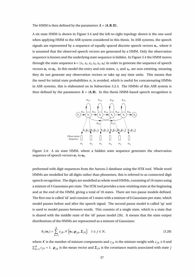
The HMM is then defined by the parametersλ= (A,B,Π).
A six state HMM is shown in Figure 3.4 and the left-to-right topology shown is the one used
when applying HMM to the ASR system considered in this thesis. In ASR systems, the speech
signals are represented by a sequence of equally spaced discrete speech vectors ot , where it
is assumed that the observed speech vectors are generated by a HMM. Only the observation
sequence is known and the underlying state sequence is hidden. In Figure 3.4 the HMM moves
through the state sequence s = {s1, s2, s3, s4, s5, s6} in order to generate the sequence of speech
vectors o1 to o6. In this model the entry and exit states, s1 and s6, are non-emitting, meaning
they do not generate any observation vectors or take up any time units. This means that
the need for initial state probabilities πi is avoided, which is useful for concatenating HMMs
in ASR systems, this is elaborated on in Subsection 3.2.4. The HMMs of this ASR system is
then defined by the parameters λ = (A,B). In this thesis HMM-based speech recognition is
a12 a23 a34 a 45 a56
a22 a33 a44 a55
1 2 3 4 5 6
a24 a35
o1 o2 o3 o4 o5 o6
b2 o1( ) b5 o6( )b2 o2( ) b3 o3( ) b4 o4( )b4 o5( )
MarkovModelM
ObservationSequence
s1 s2 s3 s4 s5 s6
Figure 3.4: A six state HMM, where a hidden state sequence generates the observationsequence of speech vectors o1 to o6.
performed with digit sequences from the Aurora-2 database using the HTK tool. Whole word
HMMs are modelled for all digits rather than phonemes, this is referred to as connected digit
speech recognition. The digits are modelled as whole word HMMs, consisting of 16 states using
a mixture of 3 Gaussians per state. The HTK tool provides a non-emitting state at the beginning
and at the end of the HMM, giving a total of 18 states. There are two pause models defined.
The first one is called ’sil’ and consists of 3 states with a mixture of 6 Gaussians per state, which
model pauses before and after the speech signal. The second pause model is called ’sp’ and
is used to model pauses between words. This consists of a single state, which is a state that
is shared with the middle state of the ’sil’ pause model [26]. It means that the state output
distributions of the HMMs are represented as a mixture of Gaussians:
b j (ot ) =K∑
k=1c j kN
(ot ;µ j k ,Σ j k
)1 ≤ j ≤ N , (3.28)
where K is the number of mixture components and c j k is the mixture weight with c j k ≥ 0 and∑Kk=1 c j k = 1. µ j k is the mean vector and Σ j k is the covariance matrix associated with state j
37
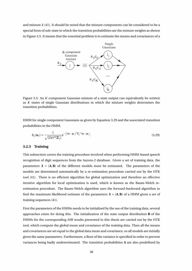
and mixture k [41]. It should be noted that the mixture components can be considered to be a
special form of sub-state in which the transition probabilities are the mixture weights as shown
in Figure 3.5. It means that the essential problem is to estimate the means and covariances of a
a ijcj1
a ijcj2
a ijcjM
...
Single Gaussians
ja ij
M-componentGaussianmixture
j1
j2
jM
K
K
K
Figure 3.5: An K -component Gaussian mixture of a state output can equivalently be writtenas K states of single Gaussian distributions in which the mixture weights determines thetransition probabilities.
HMM for single component Gaussians as given by Equation 3.29 and the associated transition
probabilities in the HMM.
b j (ot ) = 1√(2π)n |Σ j |
e−12 (ot−µ j )TΣ−1
j (ot−µ j ). (3.29)
3.2.3 Training
This subsection covers the training procedure involved when performing HMM-based speech
recognition of digit sequences from the Aurora-2 database. Given a set of training data, the
parameters λ = (A,B) of the different models must be estimated. The parameters of the
models are determined automatically by a re-estimation procedure carried out by the HTK
tool [41]. There is no efficient algorithm for global optimization and therefore an effective
iterative algorithm for local optimization is used, which is known as the Baum-Welch re-
estimation procedure. The Baum-Welch algorithm uses the forward-backward algorithm to
find the maximum likelihood estimate of the parameters λ = (A,B) of a HMM given a set of
training sequences [41].
First the parameters of the HMMs needs to be initialized by the use of the training data, several
approaches exists for doing this. The initialization of the state output distribution B of the
HMMs for the corresponding ASR results presented in this thesis are carried out by the HTK
tool, which compute the global mean and covariance of the training data. Then all the means
and covariances are set equal to the global data mean and covariance, so all models are initially
given the same parameters. Furthermore, a floor of the variance is specified in order to prevent
variances being badly underestimated. The transition probabilities A are also predefined by
38
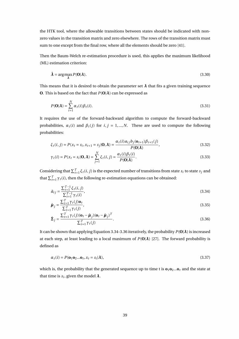
the HTK tool, where the allowable transitions between states should be indicated with non-
zero values in the transition matrix and zero elsewhere. The rows of the transition matrix must
sum to one except from the final row, where all the elements should be zero [41].
Then the Baum-Welch re-estimation procedure is used, this applies the maximum likelihood
(ML) estimation criterion:
λ= argmaxλ
P (O|λ). (3.30)
This means that it is desired to obtain the parameter set λ that fits a given training sequence
O. This is based on the fact that P (O|λ) can be expressed as
P (O|λ) =N∑
i=1αt (i )βt (i ). (3.31)
It requires the use of the forward-backward algorithm to compute the forward-backward
probabilities, αt (i ) and βt ( j ) for i , j = 1, ..., N . These are used to compute the following
probabilities:
ξt (i , j ) = P (xt = si , xt+1 = s j |O,λ) = αt (i )ai j b j (ot+1)βt+1( j )
P (O|λ), (3.32)
γt (i ) = P (xt = si |O,λ) =N∑
j=1ξt (i , j ) = αt (i )βt (i )
P (O|λ). (3.33)
Considering that∑T
t=1 ξt (i , j ) is the expected number of transitions from state si to state s j and
that∑T
t=1γt (i ), then the following re-estimation equations can be obtained:
ai j =∑T−1
t=1 ξt (i , j )∑T−1t=1 γt (i )
, (3.34)
µ j =∑T
t=1γt ( j )ot∑Tt=1γt ( j )
, (3.35)
Σ j =∑T
t=1γt ( j )(ot − µ j )(ot − µ j )T∑Tt=1γt ( j )
. (3.36)
It can be shown that applying Equation 3.34-3.36 iteratively, the probability P (O|λ) is increased
at each step, at least leading to a local maximum of P (O|λ) [27]. The forward probability is
defined as
αt (i ) = P (o1o2...ot , xt = si |λ), (3.37)
which is, the probability that the generated sequence up to time t is o1o2...ot and the state at
that time is si , given the modelλ.
39
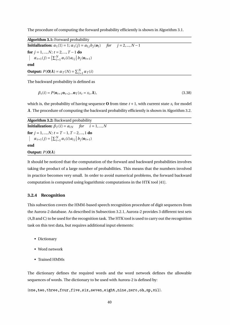
The procedure of computing the forward probability efficiently is shown in Algorithm 3.1.
Algorithm 3.1: Forward probability
Initialization: α1(1) = 1; α1( j ) = a1 j b j (o1) for j = 2, ..., N −1
for j = 1, ..., N ; t = 2, ...,T −1 do
αt+1( j ) = [∑Ni=1αt (i )ai j
]b j (ot+1)
end
Output: P (O|λ) =αT (N ) =∑Ni=1αT (i )
The backward probability is defined as
βt (i ) = P (ot+1ot+2...oT |xt = si ,λ), (3.38)
which is, the probability of having sequence O from time t +1, with current state si for model
λ. The procedure of computing the backward probability efficiently is shown in Algorithm 3.2.
Algorithm 3.2: Backward probability
Initialization: βT (i ) = ai N for i = 1, ..., N
for j = 1, ..., N ; t = T −1,T −2, ...,1 do
αt+1( j ) = [∑Ni=1αt (i )ai j
]b j (ot+1)
end
Output: P (O|λ)
It should be noticed that the computation of the forward and backward probabilities involves
taking the product of a large number of probabilities. This means that the numbers involved
in practice becomes very small. In order to avoid numerical problems, the forward backward
computation is computed using logarithmic computations in the HTK tool [41].
3.2.4 Recognition
This subsection covers the HMM-based speech recognition procedure of digit sequences from
the Aurora-2 database. As described in Subsection 3.2.1, Aurora-2 provides 3 different test sets
(A,B and C) to be used for the recognition task. The HTK tool is used to carry out the recognition
task on this test data, but requires additional input elements:
• Dictionary
• Word network
• Trained HMMs
The dictionary defines the required words and the word network defines the allowable
sequences of words. The dictionary to be used with Aurora-2 is defined by:
{one,two,three,four,five,six,seven,eight,nine,zero,oh,sp,sil}.
40
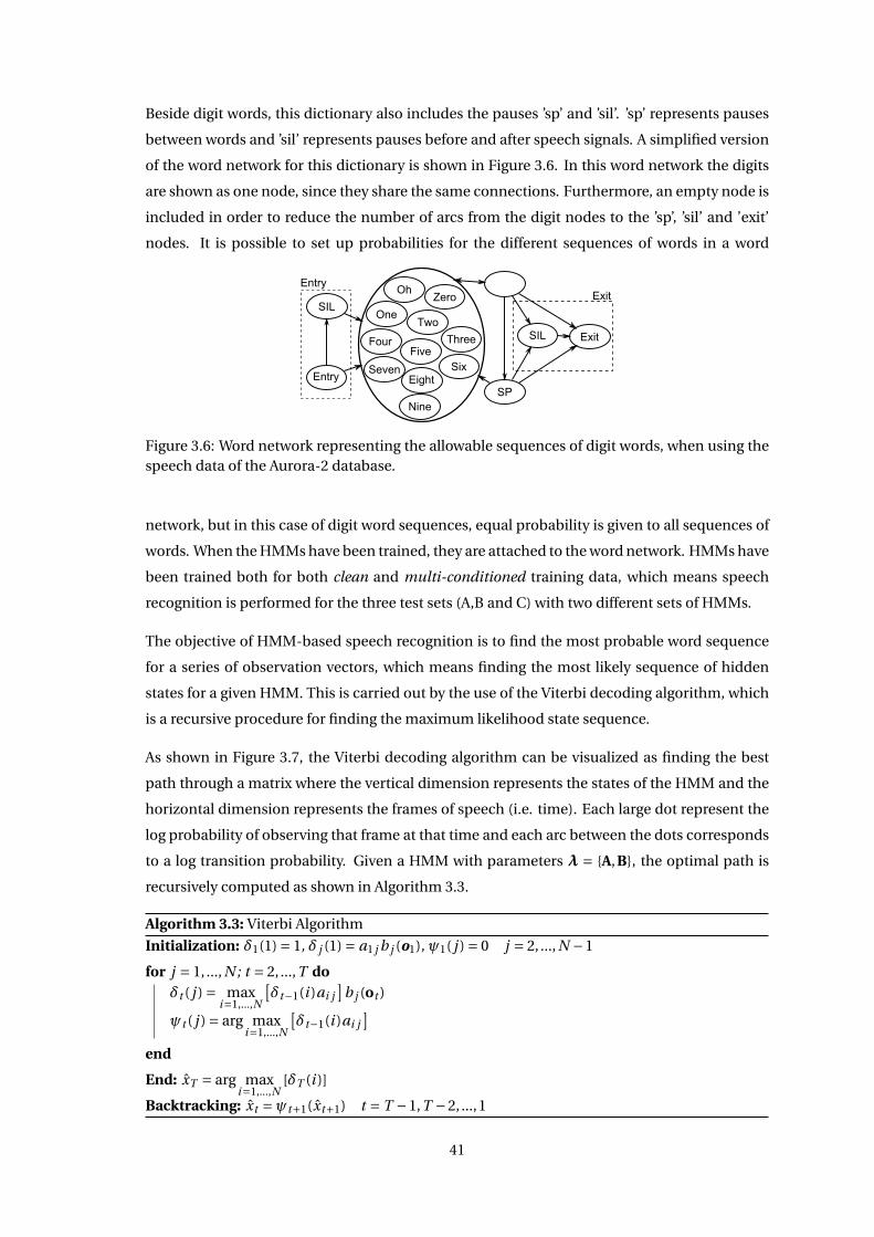
Beside digit words, this dictionary also includes the pauses ’sp’ and ’sil’. ’sp’ represents pauses
between words and ’sil’ represents pauses before and after speech signals. A simplified version
of the word network for this dictionary is shown in Figure 3.6. In this word network the digits
are shown as one node, since they share the same connections. Furthermore, an empty node is
included in order to reduce the number of arcs from the digit nodes to the ’sp’, ’sil’ and ’exit’
nodes. It is possible to set up probabilities for the different sequences of words in a word
Entry
SIL
Exit
SP
SIL
EntryExitOh
Zero
OneTwo
ThreeFour
SixFive
Seven
Nine
Eight
Figure 3.6: Word network representing the allowable sequences of digit words, when using thespeech data of the Aurora-2 database.
network, but in this case of digit word sequences, equal probability is given to all sequences of
words. When the HMMs have been trained, they are attached to the word network. HMMs have
been trained both for both clean and multi-conditioned training data, which means speech
recognition is performed for the three test sets (A,B and C) with two different sets of HMMs.
The objective of HMM-based speech recognition is to find the most probable word sequence
for a series of observation vectors, which means finding the most likely sequence of hidden
states for a given HMM. This is carried out by the use of the Viterbi decoding algorithm, which
is a recursive procedure for finding the maximum likelihood state sequence.
As shown in Figure 3.7, the Viterbi decoding algorithm can be visualized as finding the best
path through a matrix where the vertical dimension represents the states of the HMM and the
horizontal dimension represents the frames of speech (i.e. time). Each large dot represent the
log probability of observing that frame at that time and each arc between the dots corresponds
to a log transition probability. Given a HMM with parameters λ = {A,B}, the optimal path is
recursively computed as shown in Algorithm 3.3.
Algorithm 3.3: Viterbi Algorithm
Initialization: δ1(1) = 1, δ j (1) = a1 j b j (o1), ψ1( j ) = 0 j = 2, ..., N −1
for j = 1, ..., N ; t = 2, ...,T doδt ( j ) = max
i=1,...,N
[δt−1(i )ai j
]b j (ot )
ψt ( j ) = arg maxi=1,...,N
[δt−1(i )ai j
]end
End: xT = arg maxi=1,...,N
[δT (i )]
Backtracking: xt =ψt+1(xt+1) t = T −1,T −2, ...,1
41
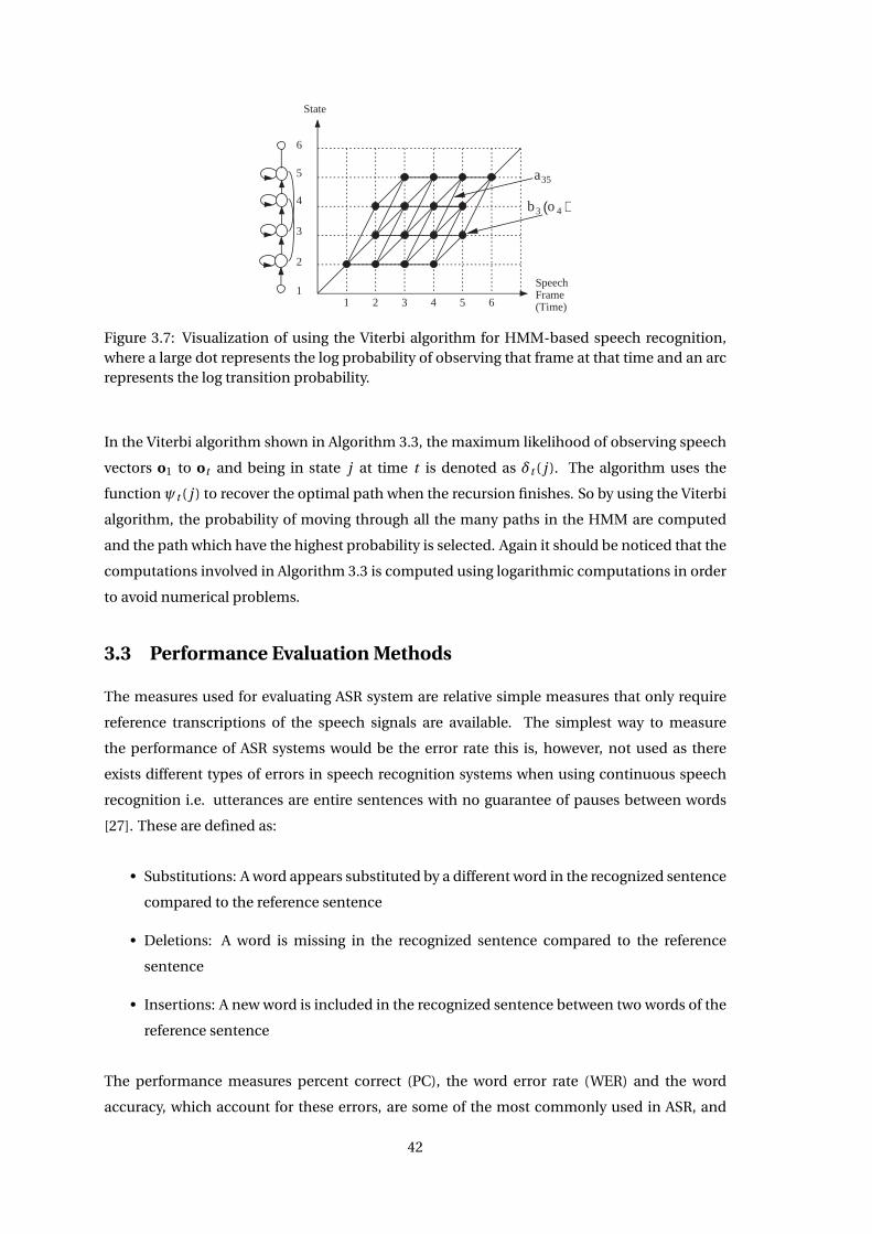
1
2
3
4
5
6
State
SpeechFrame(Time)1 2 3 4 5 6
b3 o 4( )
a35
Figure 3.7: Visualization of using the Viterbi algorithm for HMM-based speech recognition,where a large dot represents the log probability of observing that frame at that time and an arcrepresents the log transition probability.
In the Viterbi algorithm shown in Algorithm 3.3, the maximum likelihood of observing speech
vectors o1 to ot and being in state j at time t is denoted as δt ( j ). The algorithm uses the
function ψt ( j ) to recover the optimal path when the recursion finishes. So by using the Viterbi
algorithm, the probability of moving through all the many paths in the HMM are computed
and the path which have the highest probability is selected. Again it should be noticed that the
computations involved in Algorithm 3.3 is computed using logarithmic computations in order
to avoid numerical problems.
3.3 Performance Evaluation Methods
The measures used for evaluating ASR system are relative simple measures that only require
reference transcriptions of the speech signals are available. The simplest way to measure
the performance of ASR systems would be the error rate this is, however, not used as there
exists different types of errors in speech recognition systems when using continuous speech
recognition i.e. utterances are entire sentences with no guarantee of pauses between words
[27]. These are defined as:
• Substitutions: A word appears substituted by a different word in the recognized sentence
compared to the reference sentence
• Deletions: A word is missing in the recognized sentence compared to the reference
sentence
• Insertions: A new word is included in the recognized sentence between two words of the
reference sentence
The performance measures percent correct (PC), the word error rate (WER) and the word
accuracy, which account for these errors, are some of the most commonly used in ASR, and
42
are given by[27, 41]:
PC = 100 · C − I
N= N −D −S
N, (3.39)
W ER = 100 · S +D + I
N, (3.40)
WordAccuracy = 100 · N − (S +D + I )
N, (3.41)
where
• C: Number of words correctly recognized
• I: Total number of insertions
• N: Total number of evaluated words
• S: Total number of substitutions
• D: Total number of deletions
PC is often used to measure the performance of a recogniser over both words and sentences
referred to as word correct and sentence correct, respectively [41]. The sentence correct is
more sensitive to errors than the other measures, as sentences tends to contain multiple words
all of which have to be correct. Word accuracy and WER are measures of the same types of
errors, therefore only the word accuracy, word correct and sentence correct measures are used
in this thesis.
43

Speech Enhancement 4This chapter presents the speech enhancement (SE) techniques designed for human listeners,
which are used to generate the SE results within in this thesis. Furthermore the objective
performance measures used to evaluate SE of the denoised speech signals are provided.
SE aims at improving the intelligibility and/or quality of a degraded speech signal by the
use signal processing techniques [11]. The following additive signal model is considered to
represent the noisy signal in this chapter:
y(n) = x(n)+d(n), (4.1)
where y(n) is the observed noisy signal, x(n) is the unknown target signal, d(n) is the noise
signal and n is the discrete-time index [11]. Furthermore the SE methods presented in this
chapter are based on the assumptions provided in Section 1.3, where it stated that the additive
noise and the clean speech signal are statistical independent.
In this thesis it has been chosen to consider SE algorithms differentiating in their approach in
order for them to be representative of this field. The algorithms considered are: The iterative
Wiener filtering (IWF) algorithm [16], the audible noise suppression (ANS) algorithm [16] and
the short-time spectral amplitude (STSA) estimator based on the weighted euclidean (WE)
distortion measure [16]. The IWF algorithm exploits a priori assumptions of the target sound,
which is based on a speech production model. The ANS algorithm, on the other hand, exploits
assumptions on the receiver of the sound, which is based on human auditory perception and
auditory masking. The STSA WE algorithm, however, does not make any strong assumptions
about either the target signal or the receiver.
MATLAB implementations of the SE algorithms considered in this section have been provided
by [17]. These have been used for the generation of the simulation results presented in this
thesis. An overview of the MATLAB implementations are given by Appendix B.
45
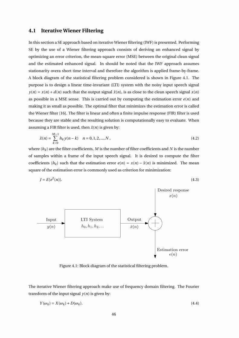
4.1 Iterative Wiener Filtering
In this section a SE approach based on iterative Wiener filtering (IWF) is presented. Performing
SE by the use of a Wiener filtering approach consists of deriving an enhanced signal by
optimizing an error criterion, the mean-square error (MSE) between the original clean signal
and the estimated enhanced signal. In should be noted that the IWF approach assumes
stationarity overa short time interval and therefore the algorithm is applied frame-by-frame.
A block diagram of the statistical filtering problem considered is shown in Figure 4.1. The
purpose is to design a linear time-invariant (LTI) system with the noisy input speech signal
y(n) = x(n)+d(n) such that the output signal x(n), is as close to the clean speech signal x(n)
as possible in a MSE sense. This is carried out by computing the estimation error e(n) and
making it as small as possible. The optimal filter that minimizes the estimation error is called
the Wiener filter [16]. The filter is linear and often a finite impulse response (FIR) filter is used
because they are stable and the resulting solution is computationally easy to evaluate. When
assuming a FIR filter is used, then x(n) is given by:
x(n) =M−1∑k=0
hk y(n −k) n = 0,1,2, ..., N , (4.2)
where {hk } are the filter coefficients, M is the number of filter coefficients and N is the number
of samples within a frame of the input speech signal. It is desired to compute the filter
coefficients {hk } such that the estimation error e(n) = x(n) − x(n) is minimized. The mean
square of the estimation error is commonly used as criterion for minimization:
J = E [e2(n)]. (4.3)
LTI System
h0, h1, h2, ...
Input
y(n)
Output
x(n)
Desired response
x(n)
Estimation errore(n)
Figure 4.1: Block diagram of the statistical filtering problem.
The iterative Wiener filtering approach make use of frequency domain filtering. The Fourier
transform of the input signal y(n) is given by:
Y (ωk ) = X (ωk )+D(ωk ). (4.4)
46
The frequency domain estimation error is defined by:
E(ωk ) = X (ωk )− X (ωk ) = X (ωk )−H(ωk )Y (ωk ). (4.5)
The optimal frequency domain filter H(ωk ) is found by computing the complex derivative of
the mean-square error J2 = E [|E(ωk )|2] with respect to H(ωk ) and setting it equal to zero:
∂J2
∂H(ωk )= 0. (4.6)
When solving Equation 4.6 for H(ωk ) the following frequency domain Wiener filter is obtained:
H(ωk ) = Pxx (ωk )
Pxx (ωk )+Pdd (ωk )= ξk
ξk +1, (4.7)
where Pxx (ωk ) = E [X (ωk )X ∗(ωk )] is the power spectrum of the clean signal x(n), Pdd (ωk ) =E [D(ωk )D∗(ωk )] is the power spectrum of the noise signal d(n) and ξk = Pxx (ωk )
Pdd (ωk ) is the a priori
SNR at frequency ωk . H(ωk ) is real, nonnegative and even, because Pxx (ωk ) ≥ 0, Pdd (ωk ) ≥ 0
and Pxx (ωk ) and Pdd (ωk ) have even symmetry. As H(ωk ) is even and real, it means that the
impulse response hk must be even as well. Therefore hk is not causal and the Wiener filter is not
realizable. Furthermore it requires knowledge about the power spectrum of the clean signal,
which is not available [16]. Therefore the Wiener filter must be estimated from the noisy signal.
The iterative Wiener filtering approach estimate the Wiener filter in an iterative procedure. An
iterative procedure is considered, where in the (i +1) iteration the enhanced signal spectrum
is estimated by:
Xi+1(ωk ) = Hi (ωk )Y (ωk ), (4.8)
where Hi (ωk ) is the Wiener filter obtained in the i th iteration. The resulting speech signal is
then assumed to be generated by an AR process where the task is to estimate the clean AR
parameters. As described in Section 2.3, the vocal tract can be modelled by a linear time-
invariant filter. The vocal tract transfer function V(z) has the following all-pole form:
V (z) = g
A(z)= g
1−∑pk=1 ak z−k
, (4.9)
where g is the gain of the system, {ak } are the all-pole coefficients and p is the number of
coefficients. The speech waveform x(n) is assumed to satisfy the following difference equation:
x(n) =p∑
k=1ak x(n −k)+ g ·w(n) n = 0,1, ..., N −1, (4.10)
where g is the gain factor and w(n) is the input excitation to the system which is assumed to
be white Gaussian noise with zero mean and unit variance. In vector notation, Equation 4.10
is given by:
x(n) = aTxp + g ·w(n), (4.11)
47
where a = [a1, a2, ..., ap ]T and xp = [x(n −1), x(n −2), ..., x(n −p)]T. But Equation 4.11 requires
initial conditions for n < p and these are denoted by xI = [x(−1), x(−2), ..., x(−p)]T. The noisy
speech signal is then given by:
y(n) = x(n)+d(n) (4.12)
= aTxp + g ·w(n)+d(n), (4.13)
where d(n) is a noise signal assumed to be white Gaussian noise with zero mean and variance
σ2d . The clean speech signal x(n) depends on 2p + 1 parameters: a, xI and g. So instead of
estimating the clean signal x(n) itself, estimation of the parameters assumed to have been used
to generate the signal is made. The iterative Wiener filtering approach performs maximum a
posteriori (MAP) estimation of the clean signal x(n) given the noisy observations y(n) and the
coefficients a, i.e. maximizing the conditional density p(x|a,y). The gain term g and the initial
conditions xI are assumed to be known. The following iterative concept has been proposed
[16]:
1. Step 1: Estimate x by maximizing p(x|a0,y) based on an initial estimate of a: a0. Denote
the first estimate of x by x1.
2. Step 2: Use x1 to make a new estimate of a denoted by a1 by the use of a linear prediction
technique. Go to step 1 and use a1 in place of a0.
This iterative procedure has been proved to converge to a local maximum of the joint
probability density p(a,x|y) [16]. Implementing step 1 in the iterative algorithm, p(x|ai ,y)
needs to be maximized over all x(n). Using Bayes’ rule, p(x|ai ,y) can be written as
p(x|ai ,y) = p(y|ai ,x)p(x|ai )
p(y|ai ), (4.14)
where ai are the coefficients obtained at the i th iteration. The denominator can be ignored as
it is not a function of x(n). It is assumed that the gain g and the initial conditions xI are known
and therefore the MAP estimate of step 1 is given by
xM AP = maxx
p(x|ai ,y) = maxx
p(y|ai ,x)p(x|ai ). (4.15)
The conditional density p(y|ai ,x) is assumed to be Gaussian with mean x(n) and variance σ2d :
p(y|ai ,x) = 1(2πσ2
d
)N /2exp
(− 1
2σ2d
N−1∑n=0
(y(n)−x(n)
)2
). (4.16)
The conditional density p(x|ai ) is also assumed Gaussian with mean aTxp and variance g 2, i.e.
it is given by:
p(x|ai ) = 1
(2πg 2)N /2exp
(− 1
2g 2
N−1∑n=0
(x(n)−aTxp )2
). (4.17)
48
By substituting Equation 4.16 and 4.17 into Equation 4.14, an expression is obtained for the
conditional density p(x|ai ,y):
p(x|ai ,y) =C1(
4π2g 2σ2d
)N /2exp
(− 1
2∆p
), (4.18)
where C is a constant and ∆p is given by:
∆p = 1
g 2
N−1∑n=0
(x(n)−aTxp
)2 + 1
σ2d
N−1∑n=0
(y(n)−x(n)
)2 . (4.19)
Maximizing p(x|ai ,y) with respect to x(n) is equivalent to minimizing ∆p , as the exponent in
Equation 4.18 is negative. x(n) is estimated by minimizing ∆p , which is carried out by taking
the derivative of ∆p with respect to x and set it equal to zero:
∂∆p
∂x(n)= 0, n = 0,1, ..., N −1. (4.20)
It can be shown that the conditional density p(x|ai ,y) is jointly Gaussian and therefore the
MAP estimate of x is equivalent to the minimum mean-square error (MMSE) estimate of x [16]
[10]. As N increases, the procedure to obtain the MMSE estimate of x given by Equation 4.20
approaches a noncausal Wiener filter. This means that the MAP estimate of x can be obtained
by filtering the noisy signal y(n) through the Wiener filter:
H(ωk ) = Pxx (ωk )
Pxx (ωk )+Pdd (ωk )= Pxx (ωk )
Pxx (ωk )+σ2d
, (4.21)
where Pxx (ω) is the power spectrum of x(n) given ai and g :
Pxx (ω) = g 2
|1−∑pk=1 ak e− j kω|2 . (4.22)
The gain g in Equation 4.22 is estimated by requiring that the variance of the noisy speech
signal, y(n), is equal to the sum of the variances of the clean signal and the noise, because x(n)
and d(n) are uncorrelated and have a mean of zero:
σ2y =σ2
x +σ2d , (4.23)
where σ2y is the variance of y(n) and σ2
x is the variance of the estimated signal x(n). The signal
variance σ2x can be computed using Parseval’s theorem:
σ2x =
N−1∑n=0
x2(n) = 1
2π
∫ π
−πPxx (ω)dω
= 1
2π
∫ π
−πg 2
|1−∑pk=1 ak e− j kω|2 dω.
(4.24)
Substituting Equation 4.24 into Equation 4.23 and solving for g 2 yields:
g 2 =2πN
∑N−1n=0 y2(n)−2πσ2
d∫ π−π
1|1−∑p
k=1 ak e− j kω|2 dω. (4.25)
49
This is used to compute the power spectrum of the clean given by Equation 4.22. The iterative
Wiener filtering algorithm is summarized in Algorithm 4.1. Again, it should be noted that the
IWF algorithm is applied frame-by-frame.
Algorithm 4.1: Iterative Wiener Filtering Algorithm [16]
Initialization: x0 = y
for i = 0,1,2, ... do(I) Given the estimated signal xi , compute the all-pole coefficients ai using the linear
prediction tecchnique.
(II) Using ai , estimate the gain term g 2 according to Equation 4.25.
(III) Compute the short-term power spectrum of the signal xi :
Pxi xi (ω) = g 2
|1−∑pk=1 ai (k)e− j kω|2 , (4.26)
where {ai (k)} are the coefficients estimated in (I).
(IV) Compute the Wiener filter:
Hi (ω) = Pxi xi (ω)
Pxi xi (ω)+σ2d
. (4.27)
(V) Estimate the spectrum of the enhanced signal:
Xi+1(ω) = Hi (ω)Y (ω), (4.28)
where Y (ω) is the spectrum of the noisy speech signal, y(n). Compute the inverse
Fourier transform of Xi+1(ω) to get the enhanced signal xi+1 in the time domain.
(VI) Go to (I) using xi+1 for the estimate signal and repeat until a converge criterion is met or
repeat for a specified number of iterations.
end
In principle, Algorithm 4.1 is run until a convergence criterion is met, but in practice the
algorithm is run for a fixed number of iterations. But determining when to terminate the
algorithm is non-trivial. It has been observed that the optimal number of iterations differ for
different types of sounds [16]. There has not been found any solution that provides the optimal
number of iterations. An example of estimated spectra for a voiced speech segment using the
IWF algorithm is shown in Figure 4.2, when running 8 iterations. It can be observed that it is not
necessarily beneficial to allow more iterations, as e.g. the two peaks at the lower frequencies
are split into two additional peaks for iteration 8 compared to iteration 3 and 4 [16].
50
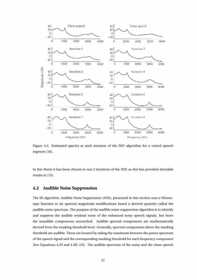
Figure 4.2: Estimated spectra at each iteration of the IWF algorithm for a voiced speech
segment [16].
In this thesis it has been chosen to run 2 iterations of the IWF, as this has provided desirable
results in [15].
4.2 Audible Noise Suppression
The SE algorithm, Audible Noise Suppression (ANS), presented in this section uses a Wiener-
type function to do spectral magnitude modifications based a derived quantity called the
audible noise spectrum. The purpose of the audible noise suppression algorithm is to identify
and suppress the audible residual noise of the enhanced noisy speech signals, but leave
the inaudible components untouched. Audible spectral components are mathematically
derived from the masking threshold level. Generally, spectral components above the masking
threshold are audible. These are located by taking the maximum between the power spectrum
of the speech signal and the corresponding masking threshold for each frequency component
(See Equations 4.29 and 4.30) [16]. The audible spectrum of the noisy and the clean speech
51
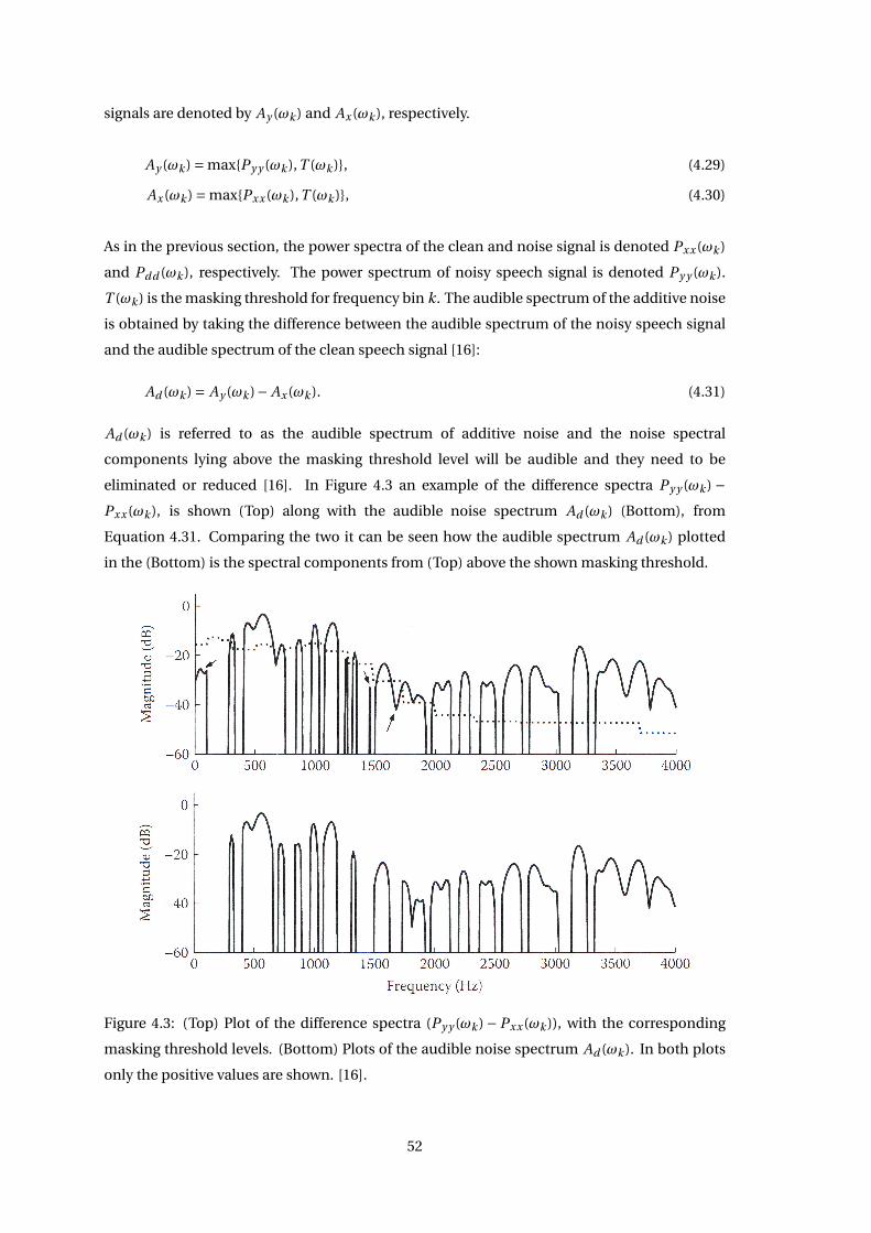
signals are denoted by Ay (ωk ) and Ax (ωk ), respectively.
Ay (ωk ) = max{Py y (ωk ),T (ωk )}, (4.29)
Ax (ωk ) = max{Pxx (ωk ),T (ωk )}, (4.30)
As in the previous section, the power spectra of the clean and noise signal is denoted Pxx (ωk )
and Pdd (ωk ), respectively. The power spectrum of noisy speech signal is denoted Py y (ωk ).
T (ωk ) is the masking threshold for frequency bin k. The audible spectrum of the additive noise
is obtained by taking the difference between the audible spectrum of the noisy speech signal
and the audible spectrum of the clean speech signal [16]:
Ad (ωk ) = Ay (ωk )− Ax (ωk ). (4.31)
Ad (ωk ) is referred to as the audible spectrum of additive noise and the noise spectral
components lying above the masking threshold level will be audible and they need to be
eliminated or reduced [16]. In Figure 4.3 an example of the difference spectra Py y (ωk ) −Pxx (ωk ), is shown (Top) along with the audible noise spectrum Ad (ωk ) (Bottom), from
Equation 4.31. Comparing the two it can be seen how the audible spectrum Ad (ωk ) plotted
in the (Bottom) is the spectral components from (Top) above the shown masking threshold.
Figure 4.3: (Top) Plot of the difference spectra (Py y (ωk ) −Pxx (ωk )), with the corresponding
masking threshold levels. (Bottom) Plots of the audible noise spectrum Ad (ωk ). In both plots
only the positive values are shown. [16].
52
The expression for Ad (ωk ) can be expanded to be more comprehensibly, which is given by:
Ad (ωk ) =
Py y (ωk )−Pxx (ωk ) if Py y (ωk ) ≥ T (ωk ) and Pxx (ωk ) ≥ T (ωk ) (I)
Py y (ωk )−T (ωk ) if Py y (ωk ) ≥ T (ωk ) and Pxx (ωk ) < T (ωk ) (II)
T (ωk )−Pxx (ωk ) if Py y (ωk ) < T (ωk ) and Pxx (ωk ) ≥ T (ωk ) (III)
0 if Py y (ωk ) < T (ωk ) and Pxx (ωk ) < T (ωk ) (IV)
. (4.32)
From Equation 4.32 it can be seen that it is only in cases I and II that the noise is audible, as
the audible noise would either be zero or negative for case III and IV [16]. Consequently, the
focus of the algorithm is to reduce the audible noise spectrum Ad (ωk ) to negative or zero by
modifying the noisy speech spectrum Py y (ωk ), thus making the residual noise inaudible. The
enhanced speech spectrum resulting from the modified Py y (ωk ) is denoted Pxx (ωk ). In order
for the noise to be inaudible the modified audible noise spectrum Ad (ωk ) must obey:
Ad (ωk ) ≤ 0, 0 ≤ k ≤ N −1, (4.33)
where N is the size of the FFT. The noisy speech spectrum is modified by a parameric Wiener-
type equation:
Pxx (ωk ) =P v(k)
y y (ωk )
αv(k)(ωk )+P v(k)y y (ωk )
Py y (ωk ). (4.34)
α(ωk ) and v(k) are time-frequency depending parameters, which are assumed to be positive.
By adjusting α(ωk ) and v(k) in Equation 4.34 the suppression of individual spectral compo-
nents can be varied. The main difference between Equation 4.34 and the Wiener filter can be
found at low SNRs, where the Wiener filter provides progressively heavier attenuation as the
SNR drops, while Equation 4.34 provides a relative constant attenuation [16]. If the parameters
α(ωk ) and v(k) are adjusted to cases I and II in Equation 4.32 then the spectral modification of
the noisy speech spectrum can achieve an optimum. By inserting Equation 4.34 into Equation
4.32 an expression for α(ωk ) and v(k) can be found that obey the constraints of case I and II:
P v(k)y y (ωk )
αv(k)(ωk )+P v(k)y y (ωk )
Py y (ωk )−Pxx (ωk ) ≤ 0, if Pxx (ωk ) ≥ T (ωk ) (I), (4.35)
P v(k)y y (ωk )
αv(k)(ωk )+P v(k)y y (ωk )
Py y (ωk )−T (ωk ) ≤ 0, if Pxx (ωk ) < T (ωk ) (II). (4.36)
The value of v(k) is fixed in order to simplify the process, so that only the value of α(ωk ) is
adaptable. If an estimation of the critical-band speech spectrum is used to find the optimal
α(ωk ) instead of relying on an estimation of the whole clean speech spectrum, a dimensional
reduction from N frequency components to B critical-band components is achieved [16]. For
the ANS algorithm there exist two proposed solutions of how to estimate the parameter α(ωk ).
The first seeks to estimate the spectral minima within each critical band. The second method
53
estimates the auditory masking threshold. This method is applied in the implementation of
the ANS algorithm [17] used in this thesis, which uses the following equation [16]:
αT (i ) = (Db(i )+T (i ))
[Db(i )
T (i )
]1/v(i )
, 1 ≤ i ≤ B , (4.37)
where B is the number of critical bands, Db(i ) and T (i ) is the noise spectrum estimation and
the masking threshold estimation in the i th critical band, respectively. v(i ) is a function of the
critical band, which is assumed to be constant within a band. Any audible noise components
are suppressed as it can be proven that Equation 4.37 obey the constraint specified in Equation
4.33 if inserted into Equation 4.35 [16]. The estimate of T (i ) is obtained using a iterative process
similar to the iterative Wiener filter described in Section 4.1, where the noisy speech signal
is passed through the suppression function expressed in Equation 4.34 multiple times with
v(i ) = 1 [16]. Each iteration produces a better estimate of the clean speech signal thus the
resulting estimation of T (i ) should also be more accurate. The iterative procedure for the j th
iteration is expressed as:
P ( j )xx (i ) = P ( j−1)
xx (i )
α( j )(i )+ P ( j−1)xx (i )
P ( j−1)xx (i ), (4.38)
where α( j )(i ) is defined as:
α( j )(i ) = D ( j−1)(i )+ (D ( j−1)(i ))2
T ( j )(i ). (4.39)
The noise power estimation for i th band at iteration j is denoted D ( j )(i ). It is initialized using
P (0)xx (i ) = Py y (i ). Power spectrum subtraction is used to process the noisy speech signal into
an estimate of the clean spectrum which is used as initial T (1)(i ) in Equation 4.39 [16]. The
algorithm based on Equation 4.37 is outlined in Algorithm 4.2.
Algorithm 4.2: Audio Noise Algorithm [16]
for all speech frames do(I) Use FFT to find the noisy speech signal power spectrum Py y (ωk ). Retain the phase of
the noisy speech spectrum.
(II) Estimate the clean power spectrum Pxx (ωk ) using power spectrum subtraction.
(III) Estimate the masking threshold T (i ) iteratively using Equations 4.38 and 4.39. Set the
initial masking threshold T (1)(i ) for Equation 4.39 using Py y (ωk ) from (II) to estimate
the masking thresholds.
(IV) In Equation 4.34 set v(i ) = 1. Then use the masking threshold from (III) to adapt
Py y (ωk ) to the constraints given by Equations 4.34 and 4.37.
(V) Use the noisy speech phase spectrum from I to calculate the inverse FFT of the
magnitude spectrum estimation from IV.
end
Objective measurements as well as subjective intelligibility measurements have been calcu-
lated for simulations run on the threshold parameters estimator. Both objective and the sub-
jective intelligibility measures showed significant improvement for ANS algorithm [16]. The
54
Diagnostic Rhyme Test 1 (DRT) was used to score the subjective intelligibility in both English
and Greek. Particular large intelligibility improvements occur at −5dB SNR [16]. The DRT for
English and Greek showed that intelligibility experienced an approximately 30% and 13% in-
crease, respectively [16].
In this thesis it has been chosen to run ANS with 2 iterations, as it has be found that no more
than 3 iteration are necessary for sufficient noise suppression [16].
4.3 Statistical Model Based Methods
In this section a statistical model based SE method is presented, which perform nonlinear
estimation of the magnitude spectrum of the clean signal using various statistical models and
optimization criteria. Initially, statistical model based SE methods are presented in general.
The parameters of interest are the DFT coefficients of the clean signal (i.e., the clean signal
spectrum). Given the DFT coefficients of the noisy signal (i.e., noisy spectrum) it is desired
to find a nonlinear estimator of the DFT coefficients of the noisy signal. There are various
techniques for deriving these nonlinear estimators including the maximum-likelihood (ML)
estimators and the Bayesian estimators [16].
Maximum-likelihood estimators and Bayesian estimators differ in the assumptions made
about the parameter of interest and the form of optimization criteria used. Bayesian estimators
assume that the parameter of interest is a random variable unlike ML estimators, which assume
that the parameter of interest is deterministic. Therefore a realization of the random variable
needs to be estimated , this approach is called Bayesian approach because its implementation
is based on Bayes’ theorem. Bayesian estimators typically perform better than the ML
estimators, as they make use of prior knowledge [16]. Therefore it has been chosen to use a
Bayesian estimator in this thesis.
General Bayesian estimators can be derived using the concept of Bayesian risk function.
Consider the sampled noisy speech signal:
y(n) = x(n)+d(n), (4.40)
which consists of the clean signal x(n) and the noise signal d(n). The noisy signal is
transformed to the time-frequency domain using the short-time Fourier transform (STFT),
which is given by:
Y (n,k) =N−1∑m=0
y(nL+m)w(m)e− j 2πN km = X (n,k)+D(n,k), (4.41)
1The DRT uses consonant-vowel-consonant sound sequence to construct monosyllabic words. These wordsare then arranged into rhyming pairs where only initial consonants differ. The DRT uses a total of ninety-sixrhyming pairs, which is arranged together in a number of groups based on distinctive speech features. Listenershave a word presented to them by the talker and is then asked to identify which word it is out of a word pair [16].
55
where k = 0,1, ..., N −1 and m denotes the frequency bin and frame index, respectively. L is the
frame shift in samples, w(m) is the analysis window and N denotes the STFT order. Expressing
Equation 4.41 in polar form
Yn,k e jθy (n,k) = Xn,k e jθx (n,k) +Dn,k e jθe (n,k), (4.42)
where {Yn,k , Xn,k ,Dn,k } denote the magnitudes and {θy (n,k),θx (n,k),θd (n,k)} denote the
phases at the kth frequency bin and at time n of the noisy speech, clean speech and noise
respectively. The purpose is to estimate the magnitude spectrum Xn,k of the clean speech
from the noisy complex speech spectrum Y (n,k). Letting ε = Xn,k − Xn,k denote the error in
estimating the magnitude spectrum Xn,k at the kth frequency bin and at time n and letting
d(ε), d(Xn,k , Xn,k ) denote a nonnegative function of ε, then the Bayes risk RB is given by
RB = E[d(Xn,k , Xn,k )
](4.43)
=∫ ∫
d(Xn,k , Xn,k )p(Xn,k ,Y (n,k))d Xn,k dY (n,k). (4.44)
Bayes risk RB is minimized with respect to Xn,k and various Bayesian estimators can be
obtained depending on the choice of the cost function. If the following squared error cost
function is used in Equation 4.44:
d(Xn,k , Xn,k ) = (Xn,k − Xn,k )2, (4.45)
then the traditional MMSE estimator E [Xn,k |Y (n,k)] is obtained when minimizing with respect
to Xn,k while holding Y (n,k) fixed. If the following cost function is used:
d(Xn,k , Xn,k ) = 0 |Xn,k − Xn,k | < δ
1 |Xn,k − Xn,k | > δ. (4.46)
then no cost is assigned for small errors (smaller than δ) and a cost of 1 is assigned for errors
larger than δ. This estimator is known as the maximum a posteriori (MAP) estimator [16].
The advantage of the risk functions is that psychoacoustic models can be integrated in the
spectral magnitude estimation. Next the Bayesian estimator considered in this thesis is
presented, which estimate the short-time spectral amplitude (STSA) of speech based on the
weighted euclidean (WE) distortion measure. This estimator is based on a replacement of the
squared error cost function with a distortion measure, which has been shown to be subjectively
more meaningful [18].
4.3.1 Bayesian Estimator Based on Weighted Euclidean Distortion Measure
In this subsection a Bayesian estimator is presented, which estimates the STSA of speech based
on a perceptually motivated cost function. This cost function is referred to as a distortion
measure [18]. A distortion measure between two vectors u ∈ RM and v ∈ RM is denoted by
d(u,v). Most distortion measures satisfy three properties:
56
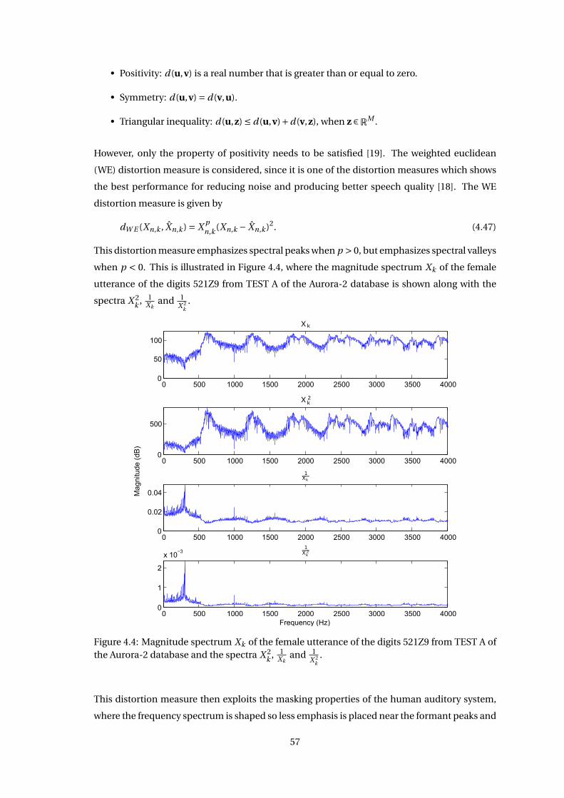
• Positivity: d(u,v) is a real number that is greater than or equal to zero.
• Symmetry: d(u,v) = d(v,u).
• Triangular inequality: d(u,z) ≤ d(u,v)+d(v,z), when z ∈RM .
However, only the property of positivity needs to be satisfied [19]. The weighted euclidean
(WE) distortion measure is considered, since it is one of the distortion measures which shows
the best performance for reducing noise and producing better speech quality [18]. The WE
distortion measure is given by
dW E (Xn,k , Xn,k ) = X pn,k (Xn,k − Xn,k )2. (4.47)
This distortion measure emphasizes spectral peaks when p > 0, but emphasizes spectral valleys
when p < 0. This is illustrated in Figure 4.4, where the magnitude spectrum Xk of the female
utterance of the digits 521Z9 from TEST A of the Aurora-2 database is shown along with the
spectra X 2k , 1
Xkand 1
X 2k
.
0 500 1000 1500 2000 2500 3000 3500 40000
50
100
Xk
0 500 1000 1500 2000 2500 3000 3500 40000
500
X 2k
0 500 1000 1500 2000 2500 3000 3500 40000
0.02
0.04
1Xk
0 500 1000 1500 2000 2500 3000 3500 40000
1
2
x 10−3
1X 2k
Frequency (Hz)
Mag
nitu
de (
dB)
Figure 4.4: Magnitude spectrum Xk of the female utterance of the digits 521Z9 from TEST A ofthe Aurora-2 database and the spectra X 2
k , 1Xk
and 1X 2
k.
This distortion measure then exploits the masking properties of the human auditory system,
where the frequency spectrum is shaped so less emphasis is placed near the formant peaks and
57
more emphasis is placed on the spectral valleys, where the amount of noise present is audible
[18]. The distortion measure considered is called weighted Euclidean distortion measure, since
it is based on the weighted Euclidean distance measure defined by:
weighted Euclidean distance =√√√√ M∑
j=1w j (u j − v j ), (4.48)
where w j are non-negative weights and u = [u1,u2, ...,uM ]T and v = [v1, v2, ..., vM ]T are two
points in M-dimensional space [9]. The weighted Euclidean distortion measure can be written
in the form of the squared weighted Euclidean distance:
dW E (Xn,k , Xn,k ) = (Xn,k − Xn,k )TW (Xn,k − Xn,k ), (4.49)
where W is a diagonal matrix with the kth diagonal element [W ]kk = X pn,k . Using Equation 4.47,
the following risk is then minimized:
R=∫ ∞
0X p
n,k (Xn,k − Xn,k )2p(Xn,k |Y (n,k))d Xn,k . (4.50)
The derivative of R with respect to Xn,k is set to zero:
∂R
∂Xn,k=
∫ ∞
0−2X p
n,k (Xn,k − Xn,k )p(Xn,k |Y (ωn,k ))d Xn,k = 0. (4.51)
Solving for Xn,k and using the Gaussian statistical model, it can be shown that Xn,k evaluates
to [16]:
Xn,k =p
vn,k
γn,k
Γ(
p+12 +1
)Φ
(− p+1
2 ,1;−vn,k
)Γ
( p2 +1
)Φ
(− p2 ,1;−vn,k
) Yn,k =Gp (ξn,k ,γn,k )Yn,k , p >−2. (4.52)
Equation 4.52 consists of a nonlinear gain function Gp (ξn,k ,γn,k ) = Xn,k
Yn,k, which is a function of
a priori SNR ξn,k and a posteriori SNR γn,k . Φ(·) and Γ(·) denotes the confluent hypergeometric
function and the gamma function which are given by Equation 4.53 and 4.54, respectively [16].
Φ(a,b; z) =∞∑
n=0
a(n)zn
b(n)n!, (4.53)
Γ(n) = (n −1)! . (4.54)
a(n) denotes the rising factorial as follows:
a(0) = 1, (4.55)
a(n) = a(a +1)(a +2) · · · (a +n −1). (4.56)
The a priori SNR ξn,k can be considered the true SNR of the kth spectral bin at time n and is
given by the ratio of the power of the clean signal and of the noise power:
ξn,k =E
[X 2
n,k
]E
[D2
n,k
] . (4.57)
58
The a posteriori SNR γn,k can be considered the observed and measured SNR of the kth spectral
bin at time n after noise is added which is given by the ratio of the squared magnitude of the
observed noisy signal and the noise power:
γn,k =Y 2
n,k
E[
D2n,k
] . (4.58)
Furthermore vn,k is given by:
vn,k = ξn,k
1+ξn,kγn,k . (4.59)
Since the clean speech signal is not available, the a priori SNR ξn,k is approximated by the use
of the decision-directed approach. The decision-directed a priori estimator is defined by the
following recursive equation [16]:
ξn,k (m) = aX 2
n,k (m −1)
E [Dn,k (m −1)2]+ (1−a)max
[γn,k (m)−1,0
], (4.60)
where 0 < a < 1 is the weighting factor, where it has been chosen to use a = 0.98 as
recommended by [16]. X 2n,k (m −1) is the amplitude estimator obtained in the previous frame.
The max(·) operator is used to ensure positiveness of the estimator, as ξn,k (m) needs to be
non-negative. Therefore the estimator of the a priori SNR ξn,k given by Equation 4.60 is a
weighted average of the past a priori SNR (given by the first term) and a present a priori SNR
estimate (given by the second term). Because of this, Equation 4.60 is called a decision-directed
estimator, since ξn,k (m) is updated using information from the previous amplitude estimate.
The following initial condition for the first frame (i.e. for m = 0) in Equation 4.60 has been
recommended by [5]:
ξn,k (0) = a + (1−a)max[γn,k (0)−1,0
]. (4.61)
In Figure 4.5 the gain function Gp (ξn,k ,γn,k ) is shown as a function of the instantaneous SNR
(γn,k −1) for a fixed value of ξn,k (ξn,k = −5dB) for several values of the power exponent p. It
is seen that the amount of attenuation is dependent on the value of the power exponent p.
Large and positive values of p provide small attenuation, whereas large and negative values of
p provide larger attenuation [18]. In this it has been chosen to a power exponent p with a value
of p = −1, which has been shown to provide a good compromise between speech distortion
and residual noise [18].
59
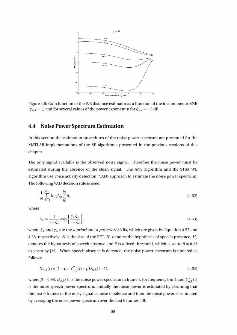
Figure 4.5: Gain function of the WE distance estimator as a function of the instantaneous SNR(γn,k −1) and for several values of the power exponent p for ξn,k =−5 dB.
4.4 Noise Power Spectrum Estimation
In this section the estimation procedures of the noise power spectrum are presented for the
MATLAB implementations of the SE algorithms presented in the previous sections of this
chapter.
The only signal available is the observed noisy signal. Therefore the noise power must be
estimated during the absence of the clean signal. The ANS algorithm and the STSA WE
algorithm use voice activity detection (VAD) approach to estimate the noise power spectrum.
The following VAD decision rule is used:
1
N
N−1∑k=1
logΛk
H1
RH0
δ, (4.62)
where
Λk = 1
1+ξkexp
{γkξk
1+ξk
}, (4.63)
where ξk and γk are the a priori and a posteriori SNRs, which are given by Equation 4.57 and
4.58, respectively. N is the size of the FFT, H1 denotes the hypothesis of speech presence, H0
denotes the hypothesis of speech absence and δ is a fixed threshold, which is set to δ = 0.15
as given by [16]. When speech absence is detected, the noise power spectrum is updated as
follows:
Dn,k (i ) = (1−β) ·Y 2n,k (i )+βDn,k (i −1), (4.64)
where β= 0.98, Dn,k (i ) is the noise power spectrum in frame i , for frequency bin k and Y 2n,k (i )
is the noise speech power spectrum. Initially the noise power is estimated by assuming that
the first 6 frames of the noisy signal is noise or silence and then the noise power is estimated
by averaging the noise power spectrum over the first 6 frames [16].
60
However, the MATLAB implementations of IWF algorithm only provides the initial estimate of
the noise power by averaging the noise power spectrum over the first 6 frames, which is fixed
for all the speech frames of the speech signal.
4.5 Performance Evaluation Methods
In this section the measures used to evaluate the performance of SE algorithms are presented.
It is not uncommon for SE algorithms to strive for improved signal quality, while simply trying
to avoid too much degradation of the speech intelligibility [16]. Therefore it is desired to
compare the effect of SE algorithms designed for human and machine receivers on both signal
quality and intelligibility. However, in order to find the true speech quality and intelligibility of
a speech signal, expensive and time consuming listening tests are required. Therefore speech
quality and intelligibility are instead estimated using the perceptual evaluation of speech
quality (PESQ) [16] and short-time objective intelligibility measure (STOI) [32], respectively.
STOI is a relative recent addition to the distortions measures used for measuring the
performance of SE algorithms. However, it has been chosen as studies have shown that it is
highly correlated with intelligibility of noisy speech and time-frequency (TF) weighted speech
signals [17, 32]. PESQ has been chosen as it is a well known industry standard [16]. Both of the
distortion measures are what is referred to as full reference algorithms, meaning they require
an original clean speech signal for comparison, in order to evaluate the degraded speech signal.
4.5.1 Short-Time Objective Intelligibility (STOI) Measure
STOI is an objective intelligibility measure designed to replace subjective listening tests, when
evaluating the effect on speech intelligibility by various SE methods, as subjective listening
tests are costly and time consuming. Specifically STOI is intended to measure any degradations
or modifications to clean/noisy speech signals brought on by a speech coder or noise reduction
schemes, where the speech signal is processed by using some type of TF varying gain function
[32].
The STOI measure is calculated using the clean and processed speech, denoted by x and y ,
respectively. It is desired that the model covers the entire frequency range relevant to speech-
intelligibility, therefore a sample-rate of 10 kHz is chosen [32]. Signals with other sample-rates
are re-sampled. In addition the method operates under the assumption that the clean and
processed speech signals are time-aligned. The signals are then segmented into frames with
a length of 256 samples, with a 50% overlap between each frame, a Hanning-window is then
applied to each frame[32]. Each frame is zero-padded up to 512 samples and the Fourier
transform is applied [32], resulting in the TF-representation of the signals. The silent frames
of the signal are then removed, as they do not contribute to speech intelligibility.
61
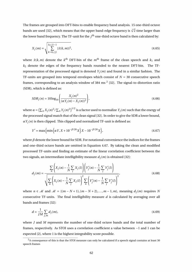
The frames are grouped into DFT-bins to enable frequency band analysis. 15 one-third octave
bands are used [32], which means that the upper band-edge frequency is 3p
2 time larger than
the lower band frequency. The TF-unit for the j th one-third octave band is then calculated by:
X j (m) =√√√√k2( j )−1∑
k=k1( j )|x(k,m)|2, (4.65)
where x(k,m) denote the kth DFT-bin of the mth frame of the clean speech and k1 and
k2 denote the edges of the frequency bands rounded to the nearest DFT-bin. The TF-
representation of the processed signal is denoted Y j (m) and found in a similar fashion. The
TF-units are grouped into temporal envelopes which consist of N = 30 consecutive speech
frames, corresponding to an analysis window of 384 ms 2 [32]. The signal-to-distortion ratio
(SDR), which is defined as:
SDR j (n) = 10log10
(X j (n)2
(αY j (n)−X j (n))2
), (4.66)
whereα= (∑n X j (n)2/
∑n Y j (n)2
)1/2is a factor used to normalize Y j (m) such that the energy of
the processed signal match that of the clean signal [32]. In order to give the SDR a lower bound,
αY j (n) is then clipped. This clipped and normalized TF-unit is defined as:
Y ′ = max(min
(αY , X +10−β/20X
)X −10−β/20X
), (4.67)
whereβ denote the lower bound for SDR. For notational convenience the indices for the frames
and one-third octave bands are omitted in Equation 4.67. By taking the clean and modified
processed TF-units and finding an estimate of the linear correlation coefficient between the
two signals, an intermediate intelligibility measure d j (m) is obtained [32]:
d j (m) =
∑n
(X j (n)− 1
N
∑l
X j (l )
)(Y ′
j (n)− 1
N
∑l
Y ′j (l )
)√√√√∑
n
(X j (n)− 1
N
∑l
X j (l )
)2 ∑n
(Y ′
j (n)− 1
N
∑l
Y ′j (l )
)2, (4.68)
where n ∈ M and M = {(m − N + 1), (m − N + 2), . . . ,m − 1,m}, meaning d j (m) requires N
consecutive TF-units. The final intelligibility measure d is calculated by averaging over all
bands and frames [32]:
d = 1
J M
∑j ,m
d j (m), (4.69)
where J and M represents the number of one-third octave bands and the total number of
frames, respectively. As STOI uses a correlation coefficient a value between −1 and 1 can be
expected [2], where 1 is the highest integrability score possible.
2A consequence of this is that the STOI measure can only be calculated if a speech signal contains at least 30speech frames
62
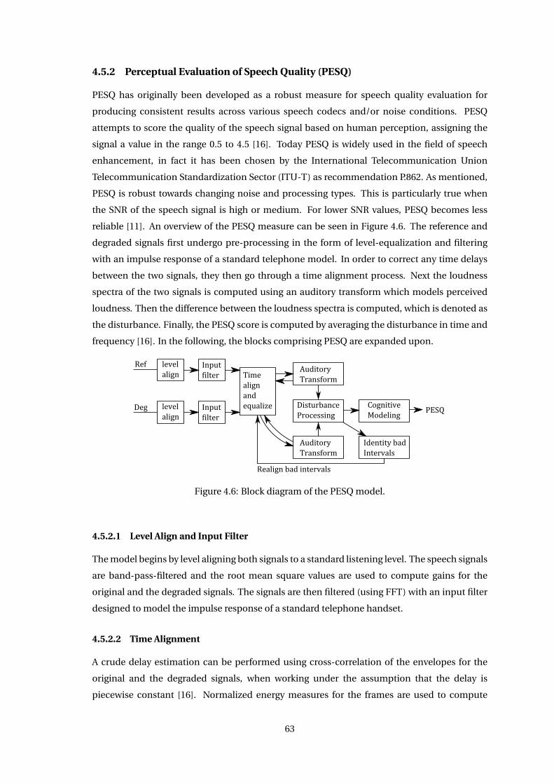
4.5.2 Perceptual Evaluation of Speech Quality (PESQ)
PESQ has originally been developed as a robust measure for speech quality evaluation for
producing consistent results across various speech codecs and/or noise conditions. PESQ
attempts to score the quality of the speech signal based on human perception, assigning the
signal a value in the range 0.5 to 4.5 [16]. Today PESQ is widely used in the field of speech
enhancement, in fact it has been chosen by the International Telecommunication Union
Telecommunication Standardization Sector (ITU-T) as recommendation P.862. As mentioned,
PESQ is robust towards changing noise and processing types. This is particularly true when
the SNR of the speech signal is high or medium. For lower SNR values, PESQ becomes less
reliable [11]. An overview of the PESQ measure can be seen in Figure 4.6. The reference and
degraded signals first undergo pre-processing in the form of level-equalization and filtering
with an impulse response of a standard telephone model. In order to correct any time delays
between the two signals, they then go through a time alignment process. Next the loudness
spectra of the two signals is computed using an auditory transform which models perceived
loudness. Then the difference between the loudness spectra is computed, which is denoted as
the disturbance. Finally, the PESQ score is computed by averaging the disturbance in time and
frequency [16]. In the following, the blocks comprising PESQ are expanded upon.
Ref
Deg
Realignbadintervals
Inputfilter
Inputfilter
levelalign
levelalign Time
alignandequalize
AuditoryTransform
AuditoryTransform
IdentitybadIntervals
DisturbanceProcessing
CognitiveModeling
PESQ
Figure 4.6: Block diagram of the PESQ model.
4.5.2.1 Level Align and Input Filter
The model begins by level aligning both signals to a standard listening level. The speech signals
are band-pass-filtered and the root mean square values are used to compute gains for the
original and the degraded signals. The signals are then filtered (using FFT) with an input filter
designed to model the impulse response of a standard telephone handset.
4.5.2.2 Time Alignment
A crude delay estimation can be performed using cross-correlation of the envelopes for the
original and the degraded signals, when working under the assumption that the delay is
piecewise constant [16]. Normalized energy measures for the frames are used to compute
63
the signal envelopes. These crude estimations are then used to separate the signals into a
number of subsections or utterances. Then the time alignment of the reference and degraded
signals is improved, first by using a crude envelope based delay estimation of the utterances
and afterwards applying Hamming windowing using a frame length of 64ms. These windows
are then cross-correlated and the sample index providing maximum correlation is taken to be
the delay estimate of each frame [16]. The confidence of the alignment for each frame is then
computed as the maximum correlation raised to the power 0.125 [16].
4.5.2.3 Auditory Transform
The signals are then processed through an auditory transform which models perceived
loudness. This involves equalising for linear filtering in the system and for gain variation. The
transform consists of the following steps:
• Bark spectrum
• Frequency equalization
• Equalisation of gain variation
• Loudness mapping
These steps are expanded upon in the following.
Bark Spectrum
The purpose of this part is to calculate the bark spectrum (the Bark frequency scale similar to
the Mel frequency scale is based on the concept of sound perception, though the scale is not as
widely used as the Mel scale). Initially an estimate of the power spectrum is found using FFT.
Windowing is carried out with the Hamming function using a frame length of 32ms and a 50 %
overlap between frames[16]. The power spectrum is then grouped into 42 bins that are equally
spaced on a modified bark scale. 49 bands are used for signals sampled at 16kHz [16].
Frequency Equalization
Working under the assumption of a constant frequency response, the transfer function is
estimated as the ratio between mean bark spectra of reference and degraded signal. The
reference signal is then equalized to degraded signal, though the equalization is limited to ±20
dB[16].
Equalisation of Gain Variation
In order to identify gain variations between frames, the ratio between the audible power of
the reference and the degraded signal in each frame is used. The ratios are then filtered using
a first order lowpass filter, H(z) = 0.8+ 0.2z−1 [16]. The filter output is then bounded to the
64
range [3×10−4,5], and finally the degraded signal is equalized to the reference signal using the
processed ratios [16].
Loudness Mapping
The bark spectrum is then mapped to the sone loudness scale (a linear scale unit for how loud
a sound is perceived):
S(b) = Sl
(P0(b)
0.5
)γ[(0.5+0.5
B ′x (b)
P0(b)
)γ−1
], (4.70)
where Sl is a loudness scaling factor, P0(b) is the hearing threshold for bark b and B ′x (b) is the
frequency compensated bark spectrum. γ is a power exponent [16].
4.5.2.4 Disturbance Processing and Cognitive Modelling
The PESQ score is computed by combining the average disturbance value and asymmetrical
disturbance value [16]. The difference in the loudness spectra between the reference signal
Sn(b) and the degraded signal Sn(b) is denoted as the raw disturbance density and it is
computed as follows:
rn(b) = Sn(b)−Sn(b), (4.71)
where, n is the frame number. The PESQ method do not square the difference, as there
is a difference between positive and negative values of the disturbance density. A positive
difference value signifies that a spectral component has been added, while a negative
difference value means that a component has been omitted[16]. However, as added
components tend to be easier perceived than omitted components, the impact on signal
quality differs [16]. A weighting scheme is applied, where omitted components are not
penalized as much as added components. An updated disturbance density Dn(b) can be
computed as
Dn(b) =
rn(b)−mn(b) if rn(b) > mn(b)
0 if |rn(b)| ≤ mn(b)
rn(b)+mn(b) if rn(b) <−mn(b)
, (4.72)
where mn(b) is defined as mn(b) = 0.25min[Sn(b),Sn(b)] [16]. An estimation of the asymmetric
effect of the differences can be found by multiplying disturbance density Dn(b) by an
asymmetry factor AFn(b) [16]. The asymmetrical disturbance density DAn is then defined as:
DAn = AFnDn(b) 1 ≤ b ≤ 42. (4.73)
The frame disturbances Dn and DAn are found by summing the disturbance density and
asymmetric density across frequency, using different norms for the disturbance density and
asymmetric density, as shown in [16]. In order to avoid incorrect time delays causing preditions
of large distortions over a small number of frames, the signal goes through a check that
65
locates any bad intervals [16]. The check is a threshold value that the frame disturbances
of consecutive frames must not be above. Afterwards any bad interval is realigned and the
frame disturbances are recomputed, now denoted as D′′n and DA′′
n [16]. Finally the disturbance
measures of the kth frame are averaged in time twice, the first averaging is defined as:
D′′′k =
(1
20
20k−1∑n=(k−1)20
(D′′
n
)6
)1/6
, (4.74)
DA′′′k =
(1
20
20k−1∑n=(k−1)20
(DA′′
n
)6
)1/6
, (4.75)
where the averaging is done over intervals of 20 frames, using 50% overlapping without
rectangular windowing [16]. Next a 2-norm is used to average the speech frames and compute
the average disturbance value dsym and the average asymmetrical disturbance value dasym,
given by:
dsym =(∑
k (D′′′k tk )2∑
k (tk )2
)1/2
, (4.76)
dasym =(∑
k (DA′′′k tk )2∑
k (tk )2
)1/2
, (4.77)
where tk are the weights applied to the frame disturbance values. The value of these weights
depend on the length of the signal [16]. Finally both the symmetrical and asymmetrical
disturbance values are jointed together as a linear combination, resulting in the final PESQ
score:
PESQ = 4.5−0.1dsym −0.0309dasym. (4.78)
As previously mentioned the range of PESQ score is 0.5 to 4.5 [16].
66
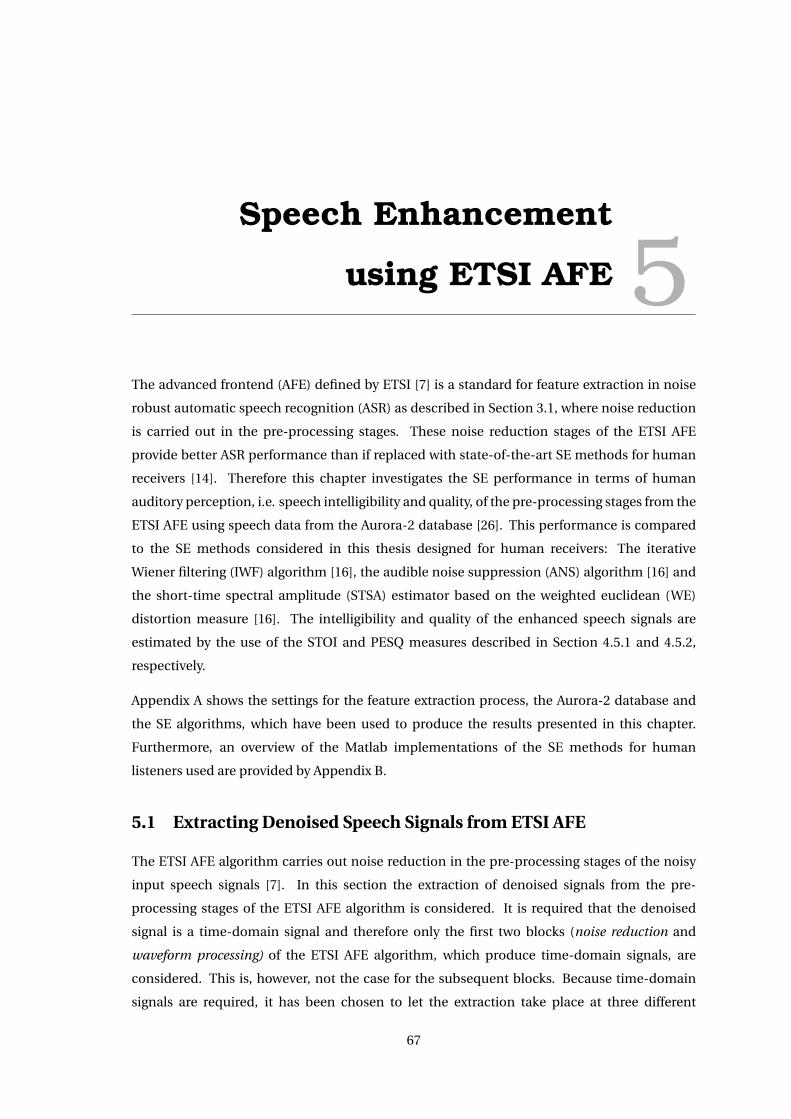
Speech Enhancement
using ETSI AFE 5The advanced frontend (AFE) defined by ETSI [7] is a standard for feature extraction in noise
robust automatic speech recognition (ASR) as described in Section 3.1, where noise reduction
is carried out in the pre-processing stages. These noise reduction stages of the ETSI AFE
provide better ASR performance than if replaced with state-of-the-art SE methods for human
receivers [14]. Therefore this chapter investigates the SE performance in terms of human
auditory perception, i.e. speech intelligibility and quality, of the pre-processing stages from the
ETSI AFE using speech data from the Aurora-2 database [26]. This performance is compared
to the SE methods considered in this thesis designed for human receivers: The iterative
Wiener filtering (IWF) algorithm [16], the audible noise suppression (ANS) algorithm [16] and
the short-time spectral amplitude (STSA) estimator based on the weighted euclidean (WE)
distortion measure [16]. The intelligibility and quality of the enhanced speech signals are
estimated by the use of the STOI and PESQ measures described in Section 4.5.1 and 4.5.2,
respectively.
Appendix A shows the settings for the feature extraction process, the Aurora-2 database and
the SE algorithms, which have been used to produce the results presented in this chapter.
Furthermore, an overview of the Matlab implementations of the SE methods for human
listeners used are provided by Appendix B.
5.1 Extracting Denoised Speech Signals from ETSI AFE
The ETSI AFE algorithm carries out noise reduction in the pre-processing stages of the noisy
input speech signals [7]. In this section the extraction of denoised signals from the pre-
processing stages of the ETSI AFE algorithm is considered. It is required that the denoised
signal is a time-domain signal and therefore only the first two blocks (noise reduction and
waveform processing) of the ETSI AFE algorithm, which produce time-domain signals, are
considered. This is, however, not the case for the subsequent blocks. Because time-domain
signals are required, it has been chosen to let the extraction take place at three different
67
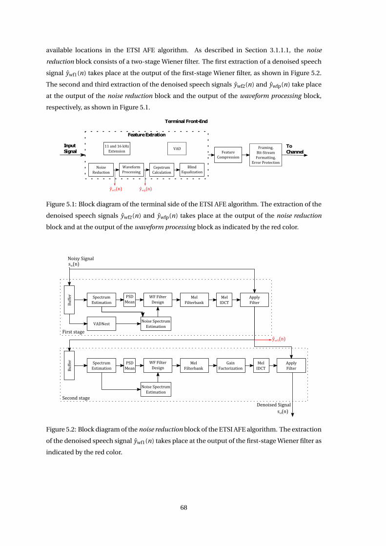
available locations in the ETSI AFE algorithm. As described in Section 3.1.1.1, the noise
reduction block consists of a two-stage Wiener filter. The first extraction of a denoised speech
signal ywf1(n) takes place at the output of the first-stage Wiener filter, as shown in Figure 5.2.
The second and third extraction of the denoised speech signals ywf2(n) and ywfp(n) take place
at the output of the noise reduction block and the output of the waveform processing block,
respectively, as shown in Figure 5.1.
ToChannel
Terminal Front-End
FeatureCompression
Framing,Bit-StreamFormatting,
Error Protection
InputSignal
FeatureExtration
CepstrumCalculation
NoizeReduction
WaveformProcessing
BlindEqualization
11 and 16 kHzExtension
VAD
ywf2(n) ywfp(n)
Figure 5.1: Block diagram of the terminal side of the ETSI AFE algorithm. The extraction of the
denoised speech signals ywf2(n) and ywfp(n) takes place at the output of the noise reduction
block and at the output of the waveform processing block as indicated by the red color.
Buffer
Buffer
GainFactorization
MelFilterbank
SpectrumEstimation
MelIDCT
ApplyFilter
WF FilterDesign
Noise SpectrumEstimation
ApplyFilter
MelFilterbank
WF FilterDesign
Noise SpectrumEstimation
VADNest
SpectrumEstimation
MelIDCT
First stage
Second stage
PSDMean
PSDMean
DenoisedSignalsof(n)
NoisySignalsin(n)
ywf1(n)
Figure 5.2: Block diagram of the noise reduction block of the ETSI AFE algorithm. The extraction
of the denoised speech signal ywf1(n) takes place at the output of the first-stage Wiener filter as
indicated by the red color.
68
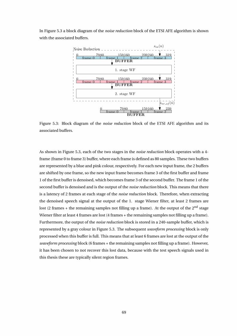
In Figure 5.3 a block diagram of the noise reduction block of the ETSI AFE algorithm is shown
with the associated buffers.
0 7980 159160 239240 319
0 7980 159160 239240 319
0 79
1. stage WF
2. stage WF
frame 1
frame 1
frame 2
frame 2
frame 3
frame 3
frame 0
frame 0
Noise Reductionsin(n)
snr of (n)
BUFFER
BUFFER
frame 0 frame 1 frame 280 159160 239
BUFFER
Figure 5.3: Block diagram of the noise reduction block of the ETSI AFE algorithm and its
associated buffers.
As shown in Figure 5.3, each of the two stages in the noise reduction block operates with a 4-
frame (frame 0 to frame 3) buffer, where each frame is defined as 80 samples. These two buffers
are represented by a blue and pink colour, respectively. For each new input frame, the 2 buffers
are shifted by one frame, so the new input frame becomes frame 3 of the first buffer and frame
1 of the first buffer is denoised, which becomes frame 3 of the second buffer. The frame 1 of the
second buffer is denoised and is the output of the noise reduction block. This means that there
is a latency of 2 frames at each stage of the noise reduction block. Therefore, when extracting
the denoised speech signal at the output of the 1. stage Wiener filter, at least 2 frames are
lost (2 frames + the remaining samples not filling up a frame). At the output of the 2nd stage
Wiener filter at least 4 frames are lost (4 frames + the remaining samples not filling up a frame).
Furthermore, the output of the noise reduction block is stored in a 240-sample buffer, which is
represented by a gray colour in Figure 5.3. The subsequent waveform processing block is only
processed when this buffer is full. This means that at least 6 frames are lost at the output of the
waveform processing block (6 frames + the remaining samples not filling up a frame). However,
it has been chosen to not recover this lost data, because with the test speech signals used in
this thesis these are typically silent region frames.
69
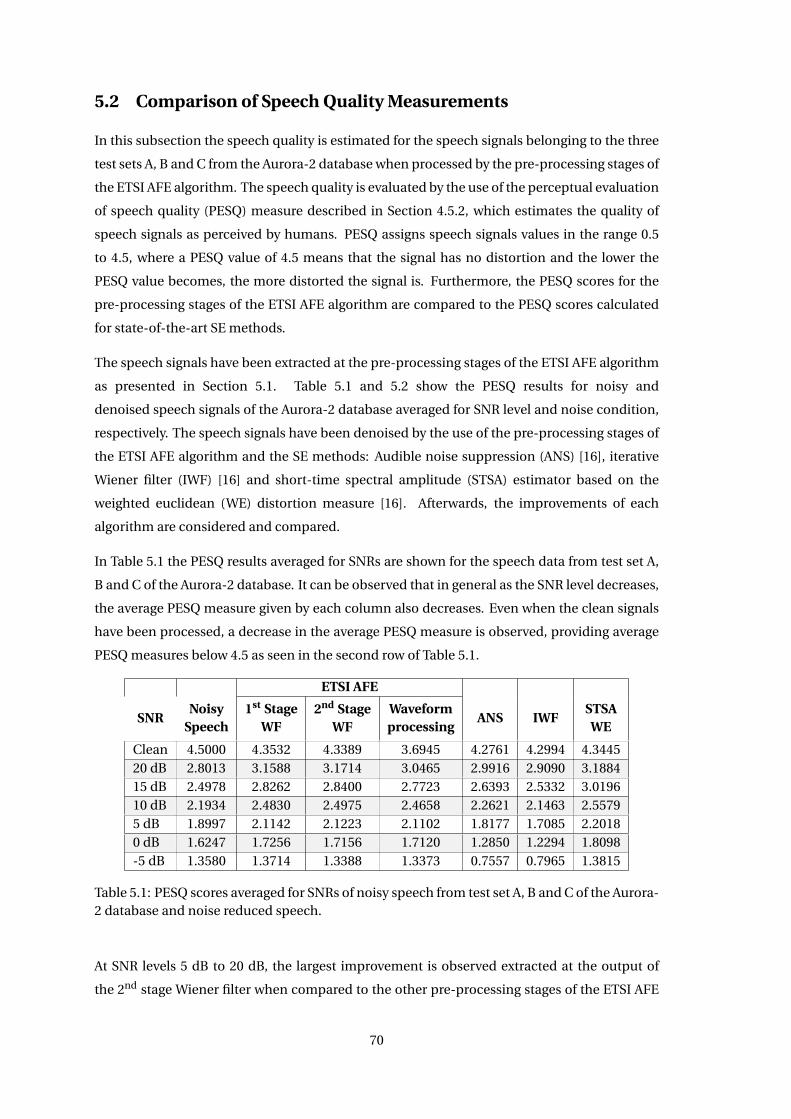
5.2 Comparison of Speech Quality Measurements
In this subsection the speech quality is estimated for the speech signals belonging to the three
test sets A, B and C from the Aurora-2 database when processed by the pre-processing stages of
the ETSI AFE algorithm. The speech quality is evaluated by the use of the perceptual evaluation
of speech quality (PESQ) measure described in Section 4.5.2, which estimates the quality of
speech signals as perceived by humans. PESQ assigns speech signals values in the range 0.5
to 4.5, where a PESQ value of 4.5 means that the signal has no distortion and the lower the
PESQ value becomes, the more distorted the signal is. Furthermore, the PESQ scores for the
pre-processing stages of the ETSI AFE algorithm are compared to the PESQ scores calculated
for state-of-the-art SE methods.
The speech signals have been extracted at the pre-processing stages of the ETSI AFE algorithm
as presented in Section 5.1. Table 5.1 and 5.2 show the PESQ results for noisy and
denoised speech signals of the Aurora-2 database averaged for SNR level and noise condition,
respectively. The speech signals have been denoised by the use of the pre-processing stages of
the ETSI AFE algorithm and the SE methods: Audible noise suppression (ANS) [16], iterative
Wiener filter (IWF) [16] and short-time spectral amplitude (STSA) estimator based on the
weighted euclidean (WE) distortion measure [16]. Afterwards, the improvements of each
algorithm are considered and compared.
In Table 5.1 the PESQ results averaged for SNRs are shown for the speech data from test set A,
B and C of the Aurora-2 database. It can be observed that in general as the SNR level decreases,
the average PESQ measure given by each column also decreases. Even when the clean signals
have been processed, a decrease in the average PESQ measure is observed, providing average
PESQ measures below 4.5 as seen in the second row of Table 5.1.
ETSI AFE
SNRNoisy
Speech1st Stage
WF2nd Stage
WFWaveformprocessing
ANS IWFSTSAWE
Clean 4.5000 4.3532 4.3389 3.6945 4.2761 4.2994 4.344520 dB 2.8013 3.1588 3.1714 3.0465 2.9916 2.9090 3.188415 dB 2.4978 2.8262 2.8400 2.7723 2.6393 2.5332 3.019610 dB 2.1934 2.4830 2.4975 2.4658 2.2621 2.1463 2.55795 dB 1.8997 2.1142 2.1223 2.1102 1.8177 1.7085 2.20180 dB 1.6247 1.7256 1.7156 1.7120 1.2850 1.2294 1.8098-5 dB 1.3580 1.3714 1.3388 1.3373 0.7557 0.7965 1.3815
Table 5.1: PESQ scores averaged for SNRs of noisy speech from test set A, B and C of the Aurora-2 database and noise reduced speech.
At SNR levels 5 dB to 20 dB, the largest improvement is observed extracted at the output of
the 2nd stage Wiener filter when compared to the other pre-processing stages of the ETSI AFE
70
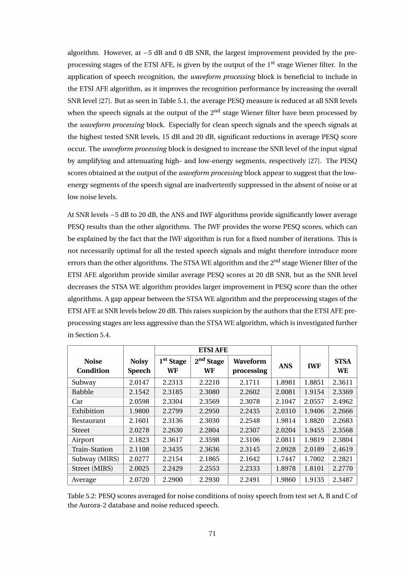
algorithm. However, at −5 dB and 0 dB SNR, the largest improvement provided by the pre-
processing stages of the ETSI AFE, is given by the output of the 1st stage Wiener filter. In the
application of speech recognition, the waveform processing block is beneficial to include in
the ETSI AFE algorithm, as it improves the recognition performance by increasing the overall
SNR level [27]. But as seen in Table 5.1, the average PESQ measure is reduced at all SNR levels
when the speech signals at the output of the 2nd stage Wiener filter have been processed by
the waveform processing block. Especially for clean speech signals and the speech signals at
the highest tested SNR levels, 15 dB and 20 dB, significant reductions in average PESQ score
occur. The waveform processing block is designed to increase the SNR level of the input signal
by amplifying and attenuating high- and low-energy segments, respectively [27]. The PESQ
scores obtained at the output of the waveform processing block appear to suggest that the low-
energy segments of the speech signal are inadvertently suppressed in the absent of noise or at
low noise levels.
At SNR levels −5 dB to 20 dB, the ANS and IWF algorithms provide significantly lower average
PESQ results than the other algorithms. The IWF provides the worse PESQ scores, which can
be explained by the fact that the IWF algorithm is run for a fixed number of iterations. This is
not necessarily optimal for all the tested speech signals and might therefore introduce more
errors than the other algorithms. The STSA WE algorithm and the 2nd stage Wiener filter of the
ETSI AFE algorithm provide similar average PESQ scores at 20 dB SNR, but as the SNR level
decreases the STSA WE algorithm provides larger improvement in PESQ score than the other
algorithms. A gap appear between the STSA WE algorithm and the preprocessing stages of the
ETSI AFE at SNR levels below 20 dB. This raises suspicion by the authors that the ETSI AFE pre-
processing stages are less aggressive than the STSA WE algorithm, which is investigated further
in Section 5.4.
ETSI AFE
NoiseCondition
NoisySpeech
1st StageWF
2nd StageWF
Waveformprocessing
ANS IWFSTSAWE
Subway 2.0147 2.2313 2.2210 2.1711 1.8981 1.8851 2.3611Babble 2.1542 2.3185 2.3080 2.2602 2.0081 1.9154 2.3369Car 2.0598 2.3304 2.3569 2.3078 2.1047 2.0557 2.4962Exhibition 1.9800 2.2799 2.2950 2.2435 2.0310 1.9406 2.2666Restaurant 2.1601 2.3136 2.3030 2.2548 1.9814 1.8820 2.2683Street 2.0278 2.2630 2.2804 2.2307 2.0204 1.9455 2.3568Airport 2.1823 2.3617 2.3598 2.3106 2.0811 1.9819 2.3804Train-Station 2.1108 2.3435 2.3636 2.3145 2.0928 2.0189 2.4619Subway (MIRS) 2.0277 2.2154 2.1865 2.1642 1.7447 1.7002 2.2821Street (MIRS) 2.0025 2.2429 2.2553 2.2333 1.8978 1.8101 2.2770
Average 2.0720 2.2900 2.2930 2.2491 1.9860 1.9135 2.3487
Table 5.2: PESQ scores averaged for noise conditions of noisy speech from test set A, B and C ofthe Aurora-2 database and noise reduced speech.
71
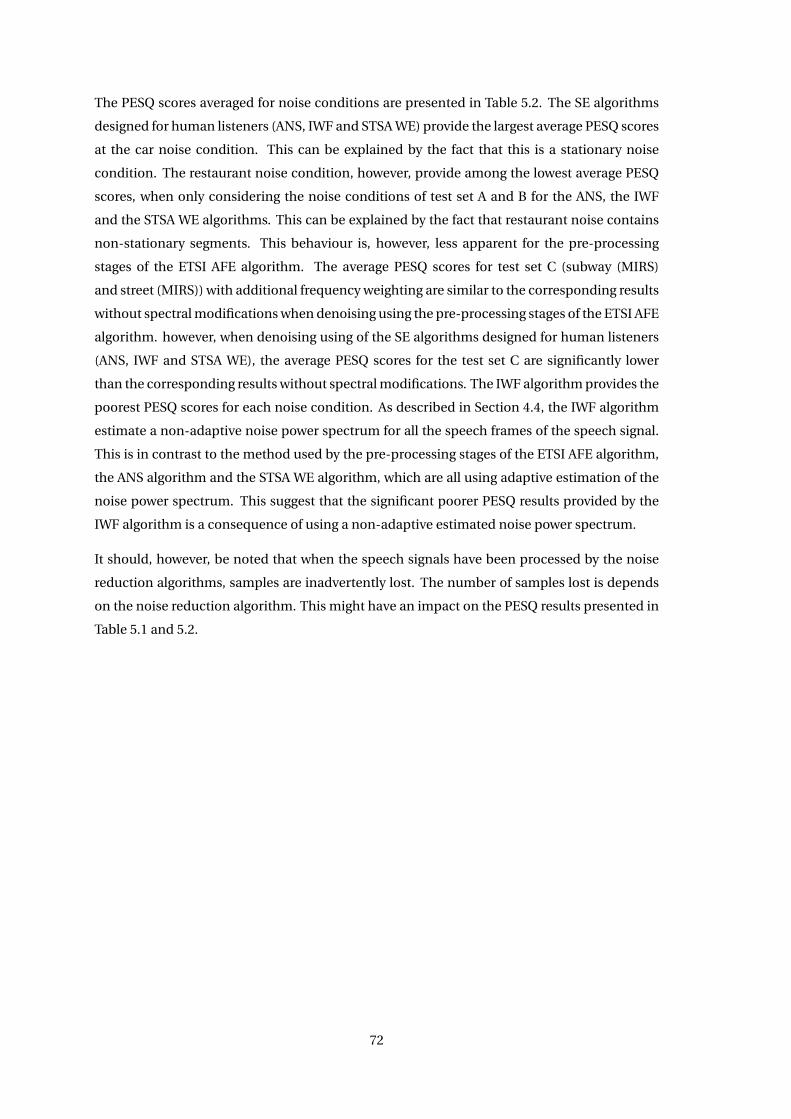
The PESQ scores averaged for noise conditions are presented in Table 5.2. The SE algorithms
designed for human listeners (ANS, IWF and STSA WE) provide the largest average PESQ scores
at the car noise condition. This can be explained by the fact that this is a stationary noise
condition. The restaurant noise condition, however, provide among the lowest average PESQ
scores, when only considering the noise conditions of test set A and B for the ANS, the IWF
and the STSA WE algorithms. This can be explained by the fact that restaurant noise contains
non-stationary segments. This behaviour is, however, less apparent for the pre-processing
stages of the ETSI AFE algorithm. The average PESQ scores for test set C (subway (MIRS)
and street (MIRS)) with additional frequency weighting are similar to the corresponding results
without spectral modifications when denoising using the pre-processing stages of the ETSI AFE
algorithm. however, when denoising using of the SE algorithms designed for human listeners
(ANS, IWF and STSA WE), the average PESQ scores for the test set C are significantly lower
than the corresponding results without spectral modifications. The IWF algorithm provides the
poorest PESQ scores for each noise condition. As described in Section 4.4, the IWF algorithm
estimate a non-adaptive noise power spectrum for all the speech frames of the speech signal.
This is in contrast to the method used by the pre-processing stages of the ETSI AFE algorithm,
the ANS algorithm and the STSA WE algorithm, which are all using adaptive estimation of the
noise power spectrum. This suggest that the significant poorer PESQ results provided by the
IWF algorithm is a consequence of using a non-adaptive estimated noise power spectrum.
It should, however, be noted that when the speech signals have been processed by the noise
reduction algorithms, samples are inadvertently lost. The number of samples lost is depends
on the noise reduction algorithm. This might have an impact on the PESQ results presented in
Table 5.1 and 5.2.
72
5.3 Comparison of Speech Intelligibility Measurements
In this subsection the speech intelligibility is estimated for the speech signals belonging to the
test sets A, B and C from the Aurora-2 database, when processed by the pre-processing stages
of the ETSI AFE algorithm and the SE algorithms designed for human receivers (ANS, IWF
and STSA WE). The speech intelligibility is estimated by the use of the short-time objective
intelligibility (STOI) measure described in Subsection 4.5.1, which is highly correlated with
intelligibility of noisy speech and time-frequency weighted noisy speech (e.g. noise reduced
speech).
The STOI measure is incalculable for speech signals containing less than 30 speech frames [32].
Consequently, the speech signals of the Aurora-2 database where less than 30 speech frames
are located by STOI, are excluded from the analysis in this thesis involving the STOI measure.
Excluding these speech signals results in an approximately 10 % reduction of the available
test data. The PESQ measure is not limited by the number of speech frames available in the
speech signals, which means all available test data is used when computing PESQ. Therefore
the exclusion of speech signals is only carried out when computing STOI.
ETSI AFE
SNRNoisy
Speech1st Stage
WF2nd Stage
WFWaveformprocessing
ANS IWFSTSAWE
Clean 1.0000 0.9995 0.9995 0.9796 0.9998 0.9999 0.999220 dB 0.9769 0.9723 0.9716 0.9546 0.9746 0.9743 0.965915 dB 0.9459 0.9436 0.9423 0.9293 0.9422 0.9408 0.931510 dB 0.8904 0.8938 0.8923 0.8841 0.8800 0.8791 0.87325 dB 0.8037 0.8144 0.8140 0.8099 0.7725 0.7764 0.78080 dB 0.6900 0.7031 0.7041 0.7021 0.6155 0.6296 0.6590-5 dB 0.5673 0.5689 0.5619 0.5604 0.4295 0.4616 0.5244
Table 5.3: STOI scores averaged for SNR levels for noisy speech from test set A, B and C of theAurora-2 database and noise reduced speech.
In Table 5.3 the STOI measures averaged for SNRs are shown for speech data from test set A,
B and C of the Aurora-2 database. It can be observed that the pre-processing stages of the
ETSI AFE algorithm provide no significant improvement or degradation of the average STOI
measure with respect to the noisy speech at any of the tested SNR levels. Except at the output
of the waveform processing block, where a small reduction in average STOI measure is observed
at the highest tested SNR levels compared to the other pre-processing stages of the ETSI AFE
algorithm. A similar observation has been obtained for the average PESQ scores, as described
in Section 5.2, which again suggests that the low-energy segments of the speech signals are
suppressed in the absent of noise or at low noise levels. At SNR levels -5 to 15 dB the 1st and
2nd stage Wiener filters of the ETSI AFE algorithm produce larger average STOI scores than
the SE algorithms designed for human receivers (ANS, IWF and STSA WE). The average STOI
73
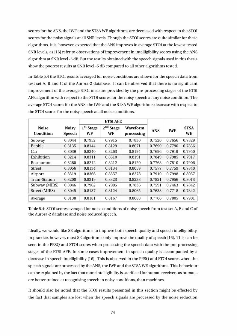
scores for the ANS, the IWF and the STSA WE algorithms are decreased with respect to the STOI
scores for the noisy signals at all SNR levels. Though the STOI scores are quite similar for these
algorithms. It is, however, expected that the ANS improves in average STOI at the lowest tested
SNR levels, as [16] refer to observations of improvement in intelligibility scores using the ANS
algorithm at SNR level -5 dB. But the results obtained with the speech signals used in this thesis
show the poorest results at SNR level -5 dB compared to all other algorithms tested.
In Table 5.4 the STOI results averaged for noise conditions are shown for the speech data from
test set A, B and C of the Aurora-2 database. It can be observed that there is no significant
improvement of the average STOI measure provided by the pre-processing stages of the ETSI
AFE algorithm with respect to the STOI scores for the noisy speech at any noise condition. The
average STOI scores for the ANS, the IWF and the STSA WE algorithms decrease with respect to
the STOI scores for the noisy speech at all noise conditions.
ETSI AFE
NoiseCondition
NoisySpeech
1st StageWF
2nd StageWF
Waveformprocessing
ANS IWFSTSAWE
Subway 0.8044 0.7952 0.7915 0.7830 0.7520 0.7656 0.7829Babble 0.8135 0.8144 0.8129 0.8071 0.7690 0.7790 0.7836Car 0.8039 0.8240 0.8263 0.8194 0.7696 0.7919 0.7950Exhibition 0.8214 0.8311 0.8310 0.8191 0.7849 0.7985 0.7917Restaurant 0.8280 0.8242 0.8212 0.8120 0.7768 0.7810 0.7906Street 0.8056 0.8134 0.8134 0.8059 0.7577 0.7759 0.7840Airport 0.8319 0.8366 0.8357 0.8278 0.7910 0.7998 0.8037Train-Station 0.8200 0.8319 0.8323 0.8238 0.7821 0.7956 0.8013Subway (MIRS) 0.8046 0.7962 0.7905 0.7836 0.7591 0.7463 0.7842Street (MIRS) 0.8045 0.8137 0.8124 0.8065 0.7638 0.7718 0.7842
Average 0.8138 0.8181 0.8167 0.8088 0.7706 0.7805 0.7901
Table 5.4: STOI scores averaged for noise conditions of noisy speech from test set A, B and C ofthe Aurora-2 database and noise reduced speech.
Ideally, we would like SE algorithms to improve both speech quality and speech intelligibility.
In practice, however, most SE algorithms only improve the quality of speech [16]. This can be
seen in the PESQ and STOI scores when processing the speech data with the pre-processing
stages of the ETSI AFE. In some cases improvement in speech quality is accompanied by a
decrease in speech intelligibility [16]. This is observed in the PESQ and STOI scores when the
speech signals are processed by the ANS, the IWF and the STSA WE algorithms. This behaviour
can be explained by the fact that more intelligibility is sacrificed for human receivers as humans
are better trained at recognising speech in noisy conditions, than machines.
It should also be noted that the STOI results presented in this section might be effected by
the fact that samples are lost when the speech signals are processed by the noise reduction
74
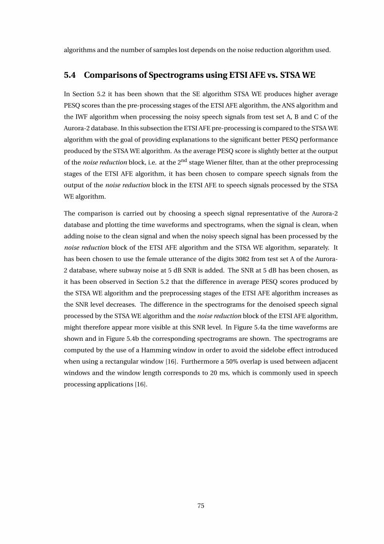
algorithms and the number of samples lost depends on the noise reduction algorithm used.
5.4 Comparisons of Spectrograms using ETSI AFE vs. STSA WE
In Section 5.2 it has been shown that the SE algorithm STSA WE produces higher average
PESQ scores than the pre-processing stages of the ETSI AFE algorithm, the ANS algorithm and
the IWF algorithm when processing the noisy speech signals from test set A, B and C of the
Aurora-2 database. In this subsection the ETSI AFE pre-processing is compared to the STSA WE
algorithm with the goal of providing explanations to the significant better PESQ performance
produced by the STSA WE algorithm. As the average PESQ score is slightly better at the output
of the noise reduction block, i.e. at the 2nd stage Wiener filter, than at the other preprocessing
stages of the ETSI AFE algorithm, it has been chosen to compare speech signals from the
output of the noise reduction block in the ETSI AFE to speech signals processed by the STSA
WE algorithm.
The comparison is carried out by choosing a speech signal representative of the Aurora-2
database and plotting the time waveforms and spectrograms, when the signal is clean, when
adding noise to the clean signal and when the noisy speech signal has been processed by the
noise reduction block of the ETSI AFE algorithm and the STSA WE algorithm, separately. It
has been chosen to use the female utterance of the digits 3082 from test set A of the Aurora-
2 database, where subway noise at 5 dB SNR is added. The SNR at 5 dB has been chosen, as
it has been observed in Section 5.2 that the difference in average PESQ scores produced by
the STSA WE algorithm and the preprocessing stages of the ETSI AFE algorithm increases as
the SNR level decreases. The difference in the spectrograms for the denoised speech signal
processed by the STSA WE algorithm and the noise reduction block of the ETSI AFE algorithm,
might therefore appear more visible at this SNR level. In Figure 5.4a the time waveforms are
shown and in Figure 5.4b the corresponding spectrograms are shown. The spectrograms are
computed by the use of a Hamming window in order to avoid the sidelobe effect introduced
when using a rectangular window [16]. Furthermore a 50% overlap is used between adjacent
windows and the window length corresponds to 20 ms, which is commonly used in speech
processing applications [16].
75
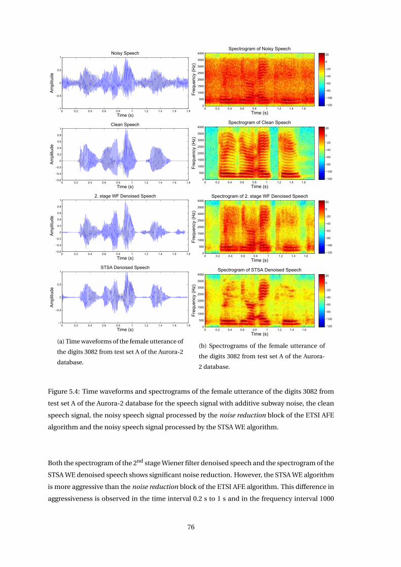
0 0.2 0.4 0.6 0.8 1 1.2 1.4 1.6 1.8−1
−0.5
0
0.5
1Noisy Speech
Time (s)
Am
plitu
de
0 0.2 0.4 0.6 0.8 1 1.2 1.4 1.6 1.8−0.6
−0.4
−0.2
0
0.2
0.4
0.6
0.8
1Clean Speech
Time (s)
Am
plitu
de
0 0.2 0.4 0.6 0.8 1 1.2 1.4 1.6 1.8−0.6
−0.4
−0.2
0
0.2
0.4
0.6
0.8
12. stage WF Denoised Speech
Time (s)
Am
plitu
de
0 0.2 0.4 0.6 0.8 1 1.2 1.4 1.6 1.8−1
−0.5
0
0.5
1STSA Denoised Speech
Time (s)
Am
plitu
de
(a) Time waveforms of the female utterance of
the digits 3082 from test set A of the Aurora-2
database.
Time (s)
Fre
quen
cy (
Hz)
Spectrogram of Noisy Speech
0 0.2 0.4 0.6 0.8 1 1.2 1.4 1.60
500
1000
1500
2000
2500
3000
3500
4000
−120
−100
−80
−60
−40
−20
0
20
Time (s)F
requ
ency
(H
z)
Spectrogram of Clean Speech
0 0.2 0.4 0.6 0.8 1 1.2 1.4 1.60
500
1000
1500
2000
2500
3000
3500
4000
−120
−100
−80
−60
−40
−20
0
20
Time (s)
Fre
quen
cy (
Hz)
Spectrogram of 2. stage WF Denoised Speech
0 0.2 0.4 0.6 0.8 1 1.2 1.4 1.60
500
1000
1500
2000
2500
3000
3500
4000
−120
−100
−80
−60
−40
−20
0
20
Time (s)
Fre
quen
cy (
Hz)
Spectrogram of STSA Denoised Speech
0 0.2 0.4 0.6 0.8 1 1.2 1.4 1.60
500
1000
1500
2000
2500
3000
3500
4000
−120
−100
−80
−60
−40
−20
0
20
(b) Spectrograms of the female utterance of
the digits 3082 from test set A of the Aurora-
2 database.
Figure 5.4: Time waveforms and spectrograms of the female utterance of the digits 3082 from
test set A of the Aurora-2 database for the speech signal with additive subway noise, the clean
speech signal, the noisy speech signal processed by the noise reduction block of the ETSI AFE
algorithm and the noisy speech signal processed by the STSA WE algorithm.
Both the spectrogram of the 2nd stage Wiener filter denoised speech and the spectrogram of the
STSA WE denoised speech shows significant noise reduction. However, the STSA WE algorithm
is more aggressive than the noise reduction block of the ETSI AFE algorithm. This difference in
aggressiveness is observed in the time interval 0.2 s to 1 s and in the frequency interval 1000
76
Hz to 3500 Hz in Figure 5.4b. This behaviour has been observed for multiple tested speech
signals of the Aurora-2 database. We deduce from this observation that the difference in SE
performance can be explained by the aggressiveness of the algorithms.
5.5 Adjustment of Aggressiveness
In Section 5.4 the ETSI AFE algorithm and the STSA WE SE algorithms have been compared
by spectrograms of speech signals from the Aurora-2 database. The results showed that the
algorithms differ in their aggressiveness of applying noise reduction. In this subsection it is
considered to investigate the impact on the word recognition accuracy using the ETSI AFE
algorithm with test set A, B and C from the Aurora-2 database, the average PESQ score and
the average STOI score of the time-domain signal at the output of the waveform processing
block, when increasing the aggressiveness of the ETSI AFE algorithm. A time-domain signal is
required to compute the PESQ and STOI scores and it have been chosen to compute the STOI
and PESQ scores from the time-domain signals at the output of the waveform processing block
as it is desired to extract the time-domain signals from within the ETSI AFE algorithm as late
as possible to get a fair impression of the word accuracy vs. PESQ and word accuracy vs. STOI
relationships.
The aggressiveness of the ETSI AFE is adjusted in the gain factorization block of the 2nd stage
Wiener filter, which is described in Subsection 3.1.1.1. The gain factorization block varies the
level of aggression from 10 % (during speech frames) to 80 % (during pure noise frames). The
level of aggression applied by the Wiener filter is therefore higher during pure noise frames [7].
The aggression during the speech frames is increased and the impact on the word accuracy vs.
the average PESQ scores and the word accuracy vs. the average STOI scores are considered.
In Figure 5.5 the word accuracy and the PESQ score averaged across SNRs -5-20 dB for speech
signals from test set A, B and C of the aurora-2 database are plotted as a function of the
aggressiveness of the speech frames, which has been varied between 10 % and 70 % with an
interval of 10 %. As expected, the word accuracy decreases and the average PESQ measure
increases as the aggressiveness applied to the speech frames increases. The increase of PESQ
measure is very small and still below the PESQ measure obtained using the STSA WE algorithm,
but it supports the concept of improving ETSI AFE for SE by introducing more aggressive noise
reduction.
77
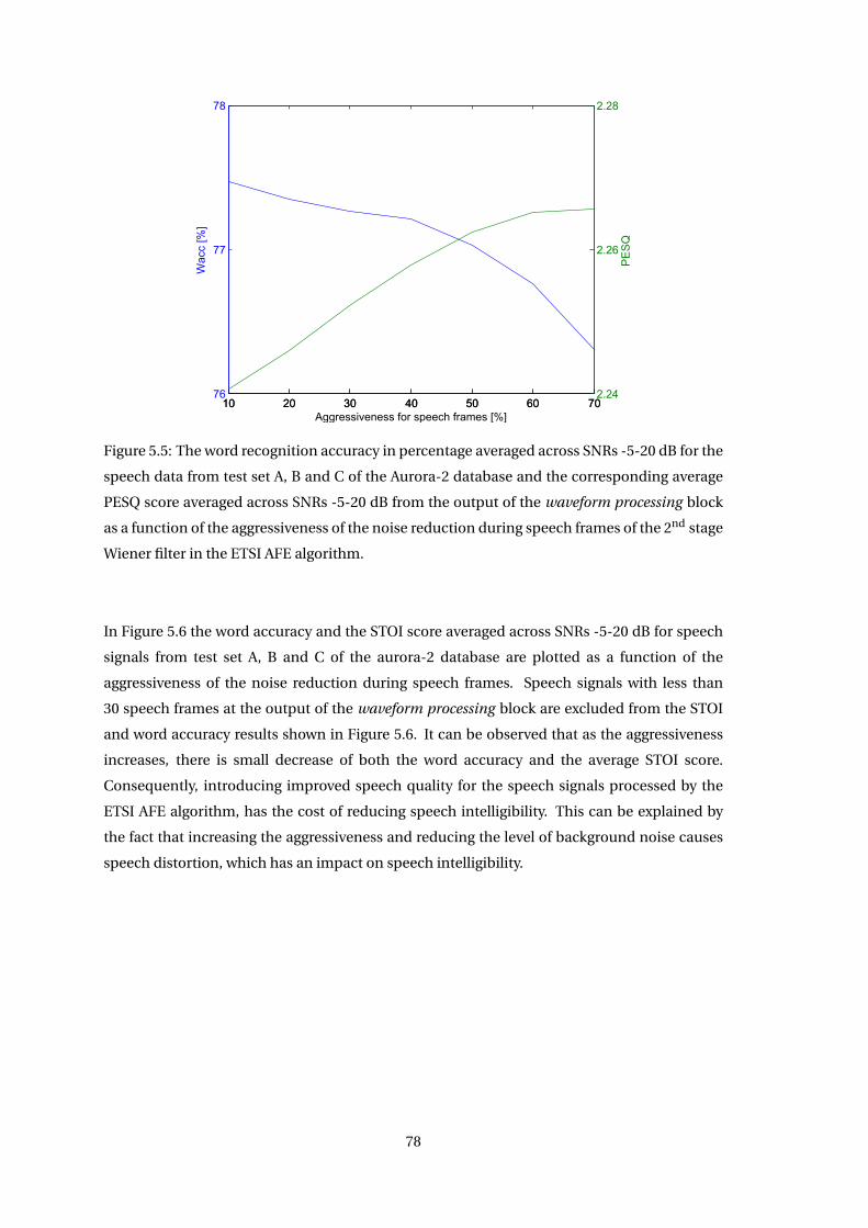
10 20 30 40 50 60 7076
77
78
Wac
c [%
]
10 20 30 40 50 60 702.24
2.26
2.28
PE
SQ
Aggressiveness for speech frames [%]
Figure 5.5: The word recognition accuracy in percentage averaged across SNRs -5-20 dB for the
speech data from test set A, B and C of the Aurora-2 database and the corresponding average
PESQ score averaged across SNRs -5-20 dB from the output of the waveform processing block
as a function of the aggressiveness of the noise reduction during speech frames of the 2nd stage
Wiener filter in the ETSI AFE algorithm.
In Figure 5.6 the word accuracy and the STOI score averaged across SNRs -5-20 dB for speech
signals from test set A, B and C of the aurora-2 database are plotted as a function of the
aggressiveness of the noise reduction during speech frames. Speech signals with less than
30 speech frames at the output of the waveform processing block are excluded from the STOI
and word accuracy results shown in Figure 5.6. It can be observed that as the aggressiveness
increases, there is small decrease of both the word accuracy and the average STOI score.
Consequently, introducing improved speech quality for the speech signals processed by the
ETSI AFE algorithm, has the cost of reducing speech intelligibility. This can be explained by
the fact that increasing the aggressiveness and reducing the level of background noise causes
speech distortion, which has an impact on speech intelligibility.
78
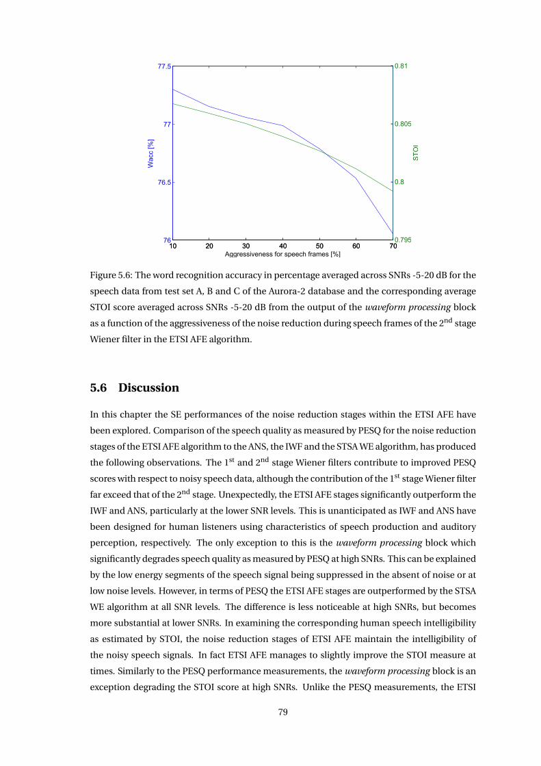
10 20 30 40 50 60 7076
76.5
77
77.5
Wac
c [%
]
10 20 30 40 50 60 700.795
0.8
0.805
0.81
ST
OI
Aggressiveness for speech frames [%]
Figure 5.6: The word recognition accuracy in percentage averaged across SNRs -5-20 dB for the
speech data from test set A, B and C of the Aurora-2 database and the corresponding average
STOI score averaged across SNRs -5-20 dB from the output of the waveform processing block
as a function of the aggressiveness of the noise reduction during speech frames of the 2nd stage
Wiener filter in the ETSI AFE algorithm.
5.6 Discussion
In this chapter the SE performances of the noise reduction stages within the ETSI AFE have
been explored. Comparison of the speech quality as measured by PESQ for the noise reduction
stages of the ETSI AFE algorithm to the ANS, the IWF and the STSA WE algorithm, has produced
the following observations. The 1st and 2nd stage Wiener filters contribute to improved PESQ
scores with respect to noisy speech data, although the contribution of the 1st stage Wiener filter
far exceed that of the 2nd stage. Unexpectedly, the ETSI AFE stages significantly outperform the
IWF and ANS, particularly at the lower SNR levels. This is unanticipated as IWF and ANS have
been designed for human listeners using characteristics of speech production and auditory
perception, respectively. The only exception to this is the waveform processing block which
significantly degrades speech quality as measured by PESQ at high SNRs. This can be explained
by the low energy segments of the speech signal being suppressed in the absent of noise or at
low noise levels. However, in terms of PESQ the ETSI AFE stages are outperformed by the STSA
WE algorithm at all SNR levels. The difference is less noticeable at high SNRs, but becomes
more substantial at lower SNRs. In examining the corresponding human speech intelligibility
as estimated by STOI, the noise reduction stages of ETSI AFE maintain the intelligibility of
the noisy speech signals. In fact ETSI AFE manages to slightly improve the STOI measure at
times. Similarly to the PESQ performance measurements, the waveform processing block is an
exception degrading the STOI score at high SNRs. Unlike the PESQ measurements, the ETSI
79
AFE stages tends to outperform each of the ANS, the IWF and the STSA WE algorithms, which
degrade the STOI score at all SNRs with respect to the noisy speech. It is not unusual for SE
algorithms designed for human receivers to sacrifice speech intelligibility for improvement of
speech quality [16]. This seems to be the case for the ANS, the IWF and the STSA WE algorithms
in terms of PESQ and STOI scores. The authors did not hear anything that contradicted this
when listening to a small number of speech signals enhanced by the different algorithms
considered in this chapter at different SNRs. Human listeners are exceptional at recognizing
speech and speech intelligibility does not typically become an issue unless the speech signal
is severely degraded. Thus improving speech quality is often considered more important than
improving speech intelligibility. The ETSI AFE stages preserve the speech intelligibility and
associated with that they show a less aggressive noise reduction performance than the STSA
WE algorithm. Machine recognisers are not nearly as proficient as humans at recognizing
speech, thus it suggests that it is more important to preserve minor details that can help the
recognisers to transcribe the speech correctly. Increasing the noise reduction aggressiveness of
the ETSI AFE has caused both the recogniser performance and the STOI measurements of the
denoised speech signal to decrease. However, the PESQ measurements increases along with
the aggressiveness. These relationships are of significant interest, as they indicate that some
correlation between the measures exists, although it is too early to tell if it is limited to ETSI
AFE.
80
ASR using Speech
Enhancement
Pre-processing Methods 6The overall objective of this chapter is to study if that the ETSI AFE algorithm feature extraction
standard designed for ASR provide higher ASR performance than when utilizing speech
enhancement algorithms designed for human receivers to pre-process the noisy speech data
for ASR as reported by [14]. The ASR results presented in this chapter have been generated
by the use of the speech data from the Aurora-2 database [26]. The SE algorithms designed
for human listeners considered in the thesis are used: The audible noise suppression (ANS)
algorithm [16], the iterative Wiener filtering (IWF) algorithm [16] and the short-time spectral
amplitude (STSA) estimator using the weighted euclidean (WE) distortion measure [16].
First, the ASR results using the ETSI AFE feature extraction standard are provided and the
contribution of the stages composing this feature extraction algorithm are evaluated. Then the
ASR performance using SE algorithms designed for human listeners for pre-processing of the
noisy speech data is investigated and compared to the ETSI AFE algorithm designed for speech
recognition. In Chapter 5 it has been found that the STSA WE algorithm differed from the
ETSI AFE algorithm by the amount of aggressiveness applied by the denoising process, where
the ETSI AFE algorithm is less aggressive. In this chapter the aggressiveness of a SE algorithm
designed for human listener is reduced with the expectation of observing an improvement in
the ASR performance. Finally, the ASR performance of the ETSI AFE algorithm and the STSA
WE algorithm is compared by removing the silence frames of the speech signals using reference
VAD labels, such that only the performance at the speech regions are compared. This is done
to investigate the contribution of the errors provided by the noisy-only regions of the speech
signals.
In this chapter recognisers are used with acoustic models trained with clean speech signals
and acoustic models trained with multi-condition (clean and noisy) speech signals, which
81
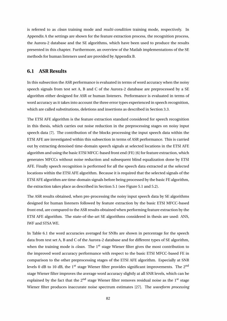
is referred to as clean training mode and multi-condition training mode, respectively. In
Appendix A the settings are shown for the feature extraction process, the recognition process,
the Aurora-2 database and the SE algorithms, which have been used to produce the results
presented in this chapter. Furthermore, an overview of the Matlab implementations of the SE
methods for human listeners used are provided by Appendix B.
6.1 ASR Results
In this subsection the ASR performance is evaluated in terms of word accuracy when the noisy
speech signals from test set A, B and C of the Aurora-2 database are preprocessed by a SE
algorithm either designed for ASR or human listeners. Performance is evaluated in terms of
word accuracy as it takes into account the three error types experienced in speech recognition,
which are called substitutions, deletions and insertions as described in Section 3.3.
The ETSI AFE algorithm is the feature extraction standard considered for speech recognition
in this thesis, which carries out noise reduction in the preprocessing stages on noisy input
speech data [7]. The contribution of the blocks processing the input speech data within the
ETSI AFE are investigated within this subsection in terms of ASR performance. This is carried
out by extracting denoised time-domain speech signals at selected locations in the ETSI AFE
algorithm and using the basic ETSI MFCC-based front end (FE) [6] for feature extraction, which
generates MFCCs without noise reduction and subsequent blind equalization done by ETSI
AFE. Finally speech recognition is performed for all the speech data extracted at the selected
locations within the ETSI AFE algorithm. Because it is required that the selected signals of the
ETSI AFE algorithm are time-domain signals before being processed by the basic FE algorithm,
the extraction takes place as described in Section 5.1 (see Figure 5.1 and 5.2).
The ASR results obtained, when pre-processing the noisy input speech data by SE algorithms
designed for human listeners followed by feature extraction by the basic ETSI MFCC-based
front end, are compared to the ASR results obtained when performing feature extraction by the
ETSI AFE algorithm. The state-of-the-art SE algorithms considered in thesis are used: ANS,
IWF and STSA WE.
In Table 6.1 the word accuracies averaged for SNRs are shown in percentage for the speech
data from test set A, B and C of the Aurora-2 database and for different types of SE algorithm,
when the training mode is clean. The 1st stage Wiener filter gives the most contribution to
the improved word accuracy performance with respect to the basic ETSI MFCC-based FE in
comparison to the other preprocessing stages of the ETSI AFE algorithm. Especially at SNR
levels 0 dB to 10 dB, the 1st stage Wiener filter provides significant improvements. The 2nd
stage Wiener filter improves the average word accuracy slightly at all SNR levels, which can be
explained by the fact that the 2nd stage Wiener filter removes residual noise as the 1st stage
Wiener filter produces inaccurate noise spectrum estimates [27]. The waveform processing
82
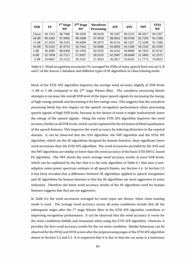
SNR FE1st Stage
WF2nd Stage
WFWaveformProcessing
AFE ANS IWFSTSAWE
Clean 99.1533 98.7900 99.2050 98.9450 99.2367 98.5233 98.5017 99.226720 dB 96.4383 97.9992 98.1000 97.9250 98.0642 89.5700 82.7283 95.130015 dB 91.3433 96.5525 96.6900 96.5875 96.6142 80.1267 72.5208 91.150810 dB 76.5433 91.9733 92.7942 92.6600 93.0692 64.1308 59.1542 82.53505 dB 49.4983 80.6408 82.1950 82.9192 84.4242 40.8808 40.7833 65.97420 dB 22.7058 55.7517 57.9267 59.2325 62.2867 20.0400 21.5883 41.2375-5 dB 10.6667 25.5125 26.3167 27.3633 30.3817 10.8342 11.7775 19.0933
Table 6.1: Word recognition accuracies [%] averaged for SNRs of noisy speech from test set A, Band C of the Aurora-2 database and different types of SE algorithms in clean training mode.
block of the ETSI AFE algorithm improves the average word accuracy slightly at SNR levels
-5 dB to 5 dB compared to the 2nd stage Wiener filter. The waveform processing blocks
attempts to increase the overall SNR level of the input speech signals by increasing the energy
of high-energy periods and decreasing it for low-energy ones. This suggests that the waveform
processing block has less impact on the speech recognition performance when processing
speech signals of high SNR levels, because in the absent of noise it might inadvertently lower
the energy of the speech signals. Using the entire ETSI AFE algorithm improves the word
accuracy further at all SNR levels, which can be explained by the inclusion of blind equalisation
of the speech features. This improves the word accuracy by reducing distortion in the cepstral
domain. It can be observed that the ANS algorithm, the IWF algorithm and the STSA WE
algorithm, which are the SE algorithms designed for human listeners, show significant lower
word accuracies than the ETSI AFE algorithm. The word accuracies provided by the ANS and
the IWF algorithms are similar or lower than the word accuracy of the basic ETSI MFCC-based
FE algorithm. The IWF shows the worst average word accuracy results at most SNR levels,
which can be explained by the fact that it is the only algorithm of Table 6.1 that uses a non-
adaptive noise power spectrum estimate at all speech frames, see Section 4.4. In Section 5.5
it has been revealed that a difference between SE algorithms applied to speech recognition
and SE algorithms for human listeners is that the SE algorithms are more aggressive in noise
reduction. Therefore the lower word accuracy results of the SE algorithms used for human
listeners suggests that they are too aggressive.
In Table 6.2 the word accuracies averaged for noise types are shown, when clean training
mode is used. The average word accuracy across all noise conditions reveals that all the
subsequent stages after the 1st stage Wiener filter in the ETSI AFE algorithm contribute to
improving recognition performance. It can be observed that the word accuracy is worse for
the noise conditions babble and restaurant when using the ETSI AFE algorithm. However, it
provides the best word accuracy results for the car noise condition. Similar behaviour can be
observed for the PESQ and STOI scores after the preprocessing stages of the ETSI AFE algorithm
shown in Section 5.2 and 5.3. It is suspected that it is due to that the car noise is a stationary
83
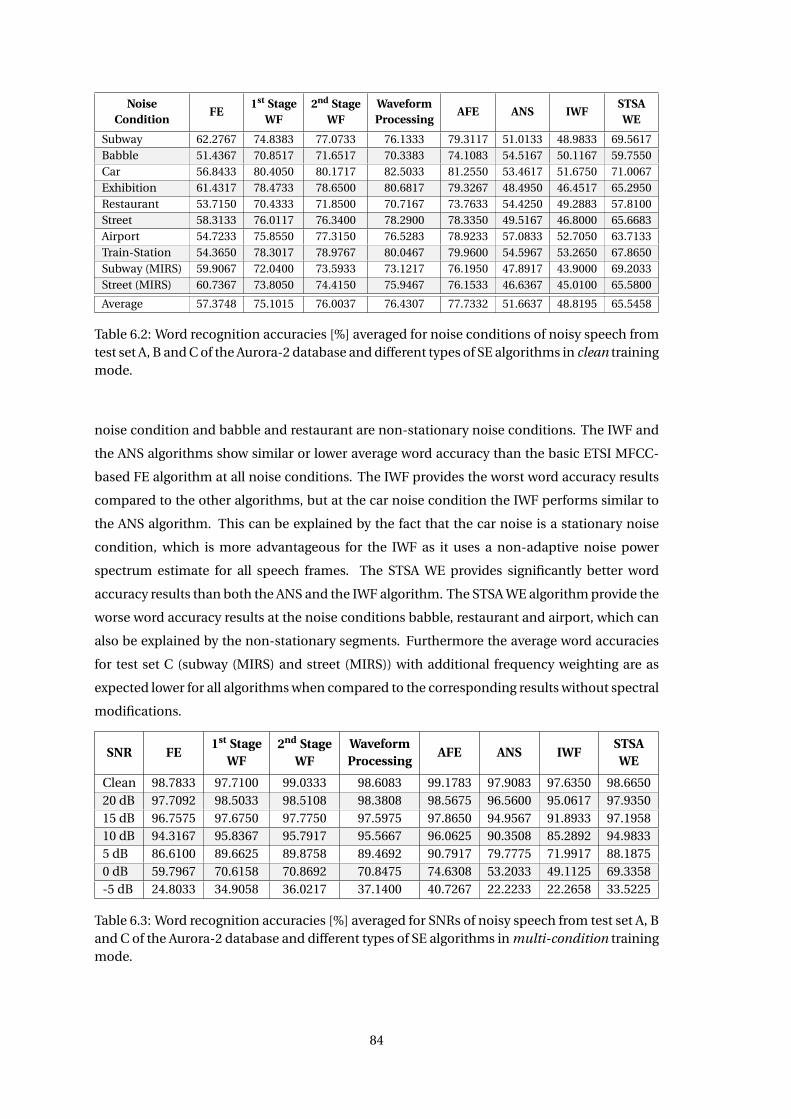
NoiseCondition
FE1st Stage
WF2nd Stage
WFWaveformProcessing
AFE ANS IWFSTSAWE
Subway 62.2767 74.8383 77.0733 76.1333 79.3117 51.0133 48.9833 69.5617Babble 51.4367 70.8517 71.6517 70.3383 74.1083 54.5167 50.1167 59.7550Car 56.8433 80.4050 80.1717 82.5033 81.2550 53.4617 51.6750 71.0067Exhibition 61.4317 78.4733 78.6500 80.6817 79.3267 48.4950 46.4517 65.2950Restaurant 53.7150 70.4333 71.8500 70.7167 73.7633 54.4250 49.2883 57.8100Street 58.3133 76.0117 76.3400 78.2900 78.3350 49.5167 46.8000 65.6683Airport 54.7233 75.8550 77.3150 76.5283 78.9233 57.0833 52.7050 63.7133Train-Station 54.3650 78.3017 78.9767 80.0467 79.9600 54.5967 53.2650 67.8650Subway (MIRS) 59.9067 72.0400 73.5933 73.1217 76.1950 47.8917 43.9000 69.2033Street (MIRS) 60.7367 73.8050 74.4150 75.9467 76.1533 46.6367 45.0100 65.5800
Average 57.3748 75.1015 76.0037 76.4307 77.7332 51.6637 48.8195 65.5458
Table 6.2: Word recognition accuracies [%] averaged for noise conditions of noisy speech fromtest set A, B and C of the Aurora-2 database and different types of SE algorithms in clean trainingmode.
noise condition and babble and restaurant are non-stationary noise conditions. The IWF and
the ANS algorithms show similar or lower average word accuracy than the basic ETSI MFCC-
based FE algorithm at all noise conditions. The IWF provides the worst word accuracy results
compared to the other algorithms, but at the car noise condition the IWF performs similar to
the ANS algorithm. This can be explained by the fact that the car noise is a stationary noise
condition, which is more advantageous for the IWF as it uses a non-adaptive noise power
spectrum estimate for all speech frames. The STSA WE provides significantly better word
accuracy results than both the ANS and the IWF algorithm. The STSA WE algorithm provide the
worse word accuracy results at the noise conditions babble, restaurant and airport, which can
also be explained by the non-stationary segments. Furthermore the average word accuracies
for test set C (subway (MIRS) and street (MIRS)) with additional frequency weighting are as
expected lower for all algorithms when compared to the corresponding results without spectral
modifications.
SNR FE1st Stage
WF2nd Stage
WFWaveformProcessing
AFE ANS IWFSTSAWE
Clean 98.7833 97.7100 99.0333 98.6083 99.1783 97.9083 97.6350 98.665020 dB 97.7092 98.5033 98.5108 98.3808 98.5675 96.5600 95.0617 97.935015 dB 96.7575 97.6750 97.7750 97.5975 97.8650 94.9567 91.8933 97.195810 dB 94.3167 95.8367 95.7917 95.5667 96.0625 90.3508 85.2892 94.98335 dB 86.6100 89.6625 89.8758 89.4692 90.7917 79.7775 71.9917 88.18750 dB 59.7967 70.6158 70.8692 70.8475 74.6308 53.2033 49.1125 69.3358-5 dB 24.8033 34.9058 36.0217 37.1400 40.7267 22.2233 22.2658 33.5225
Table 6.3: Word recognition accuracies [%] averaged for SNRs of noisy speech from test set A, Band C of the Aurora-2 database and different types of SE algorithms in multi-condition trainingmode.
84
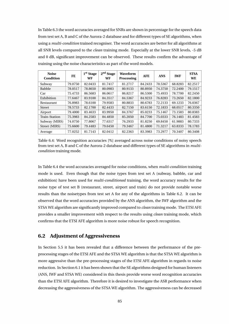
In Table 6.3 the word accuracies averaged for SNRs are shown in percentage for the speech data
from test set A, B and C of the Aurora-2 database and for different types of SE algorithms, when
using a multi-condition trained recogniser. The word accuracies are better for all algorithms at
all SNR levels compared to the clean training mode. Especially at the lower SNR levels, -5 dB
and 0 dB, significant improvement can be observed. These results confirm the advantage of
training using the noise characteristics as part of the word models.
NoiseCondition
FE1st Stage
WF2nd Stage
WFWaveformProcessing
AFE ANS IWFSTSAWE
Subway 79.0750 82.0433 81.7417 81.2717 84.2433 70.5367 68.8283 82.2517Babble 78.0517 78.8650 80.0983 80.9133 80.8950 74.3750 72.2400 79.1517Car 75.4733 86.5683 86.0617 86.8217 86.5300 75.4933 78.7700 82.2450Exhibition 77.6467 83.9100 84.3517 84.5367 84.9233 76.8283 73.2650 82.1800Restaurant 76.8983 78.6100 79.9583 80.8833 80.6783 72.2133 69.1233 76.0367Street 78.5733 82.1700 82.4433 82.7150 83.6150 72.1833 68.0517 80.3350Airport 79.4000 83.4633 83.9950 84.3767 85.0233 75.1467 73.1583 80.8383Train-Station 75.3983 84.2583 84.4850 85.2050 84.7700 75.0333 76.1483 81.4583Subway (MIRS) 74.0750 77.8067 77.6317 76.2933 81.8250 69.8450 61.9883 80.7333Street (MIRS) 75.6600 79.4483 79.6450 79.3467 81.4800 71.3217 63.8333 78.1783
Average 77.0252 81.7143 82.0412 82.2363 83.3983 73.2977 70.3407 80.3408
Table 6.4: Word recognition accuracies [%] averaged across noise conditions of noisy speechfrom test set A, B and C of the Aurora-2 database and different types of SE algorithms in multi-condition training mode.
In Table 6.4 the word accuracies averaged for noise conditions, when multi-condition training
mode is used. Even though that the noise types from test set A (subway, babble, car and
exhibition) have been used for multi-conditioned training, the word accuracy results for the
noise type of test set B (restaurant, street, airport and train) do not provide notable worse
results than the noisetypes from test set A for any of the algorithms in Table 6.2. It can be
observed that the word accuracies provided by the ANS algorithm, the IWF algorithm and the
STSA WE algorithm are significantly improved compared to clean training mode. The ETSI AFE
provides a smaller improvement with respect to the results using clean training mode, which
confirms that the ETSI AFE algorithm is more noise robust for speech recognition.
6.2 Adjustment of Aggressiveness
In Section 5.5 it has been revealed that a difference between the performance of the pre-
processing stages of the ETSI AFE and the STSA WE algorithm is that the STSA WE algorithm is
more aggressive than the pre-processing stages of the ETSI AFE algorithm in regards to noise
reduction. In Section 6.1 it has been shown that the SE algorithms designed for human listeners
(ANS, IWF and STSA WE) considered in this thesis provide worse word recognition accuracies
than the ETSI AFE algorithm. Therefore it is desired to investigate the ASR performance when
decreasing the aggressiveness of the STSA WE algorithm. The aggressiveness can be decreased
85
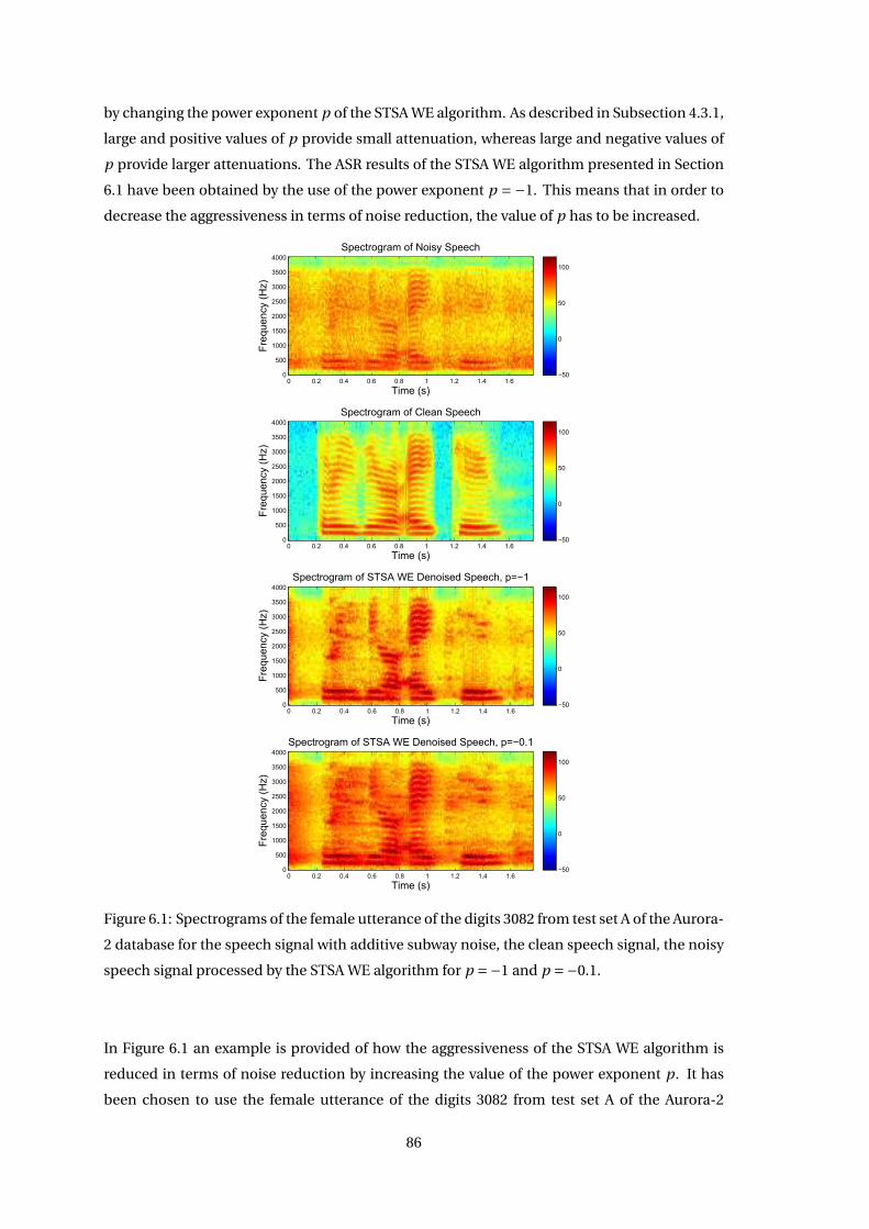
by changing the power exponent p of the STSA WE algorithm. As described in Subsection 4.3.1,
large and positive values of p provide small attenuation, whereas large and negative values of
p provide larger attenuations. The ASR results of the STSA WE algorithm presented in Section
6.1 have been obtained by the use of the power exponent p = −1. This means that in order to
decrease the aggressiveness in terms of noise reduction, the value of p has to be increased.
Time (s)
Fre
quen
cy (
Hz)
Spectrogram of Noisy Speech
0 0.2 0.4 0.6 0.8 1 1.2 1.4 1.60
500
1000
1500
2000
2500
3000
3500
4000
−50
0
50
100
Time (s)
Fre
quen
cy (
Hz)
Spectrogram of Clean Speech
0 0.2 0.4 0.6 0.8 1 1.2 1.4 1.60
500
1000
1500
2000
2500
3000
3500
4000
−50
0
50
100
Time (s)
Fre
quen
cy (
Hz)
Spectrogram of STSA WE Denoised Speech, p=−1
0 0.2 0.4 0.6 0.8 1 1.2 1.4 1.60
500
1000
1500
2000
2500
3000
3500
4000
−50
0
50
100
Time (s)
Fre
quen
cy (
Hz)
Spectrogram of STSA WE Denoised Speech, p=−0.1
0 0.2 0.4 0.6 0.8 1 1.2 1.4 1.60
500
1000
1500
2000
2500
3000
3500
4000
−50
0
50
100
Figure 6.1: Spectrograms of the female utterance of the digits 3082 from test set A of the Aurora-
2 database for the speech signal with additive subway noise, the clean speech signal, the noisy
speech signal processed by the STSA WE algorithm for p =−1 and p =−0.1.
In Figure 6.1 an example is provided of how the aggressiveness of the STSA WE algorithm is
reduced in terms of noise reduction by increasing the value of the power exponent p. It has
been chosen to use the female utterance of the digits 3082 from test set A of the Aurora-2
86
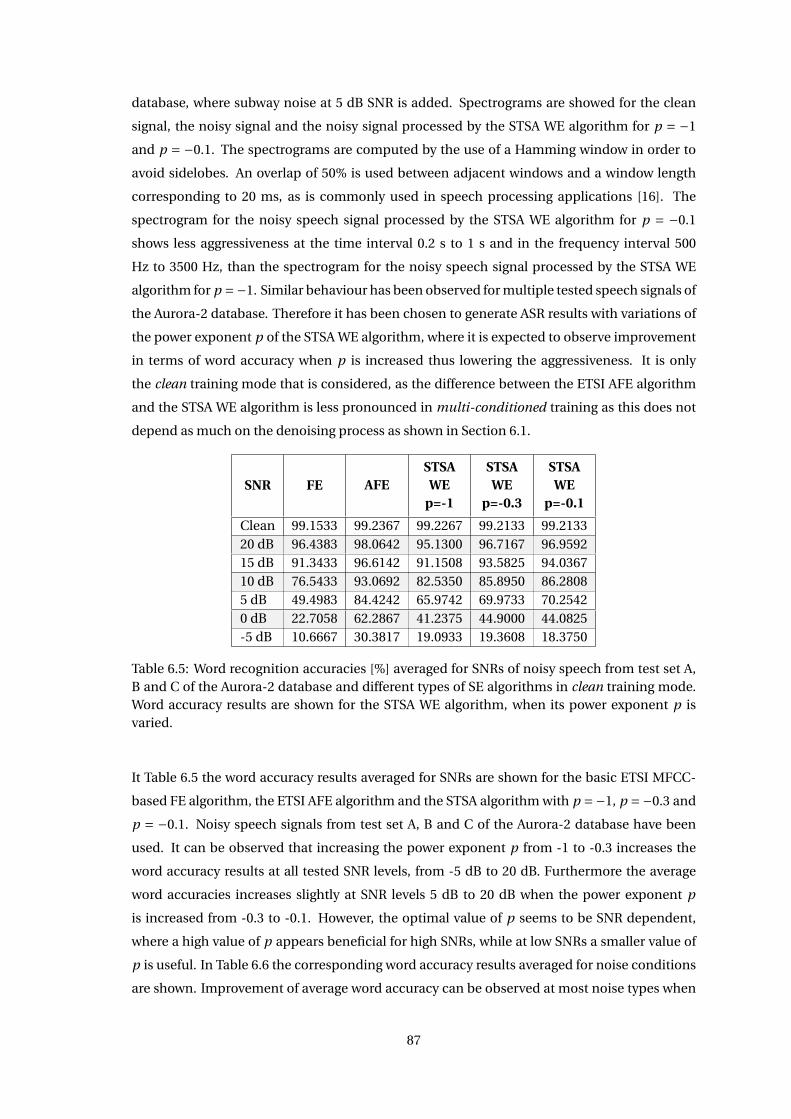
database, where subway noise at 5 dB SNR is added. Spectrograms are showed for the clean
signal, the noisy signal and the noisy signal processed by the STSA WE algorithm for p = −1
and p = −0.1. The spectrograms are computed by the use of a Hamming window in order to
avoid sidelobes. An overlap of 50% is used between adjacent windows and a window length
corresponding to 20 ms, as is commonly used in speech processing applications [16]. The
spectrogram for the noisy speech signal processed by the STSA WE algorithm for p = −0.1
shows less aggressiveness at the time interval 0.2 s to 1 s and in the frequency interval 500
Hz to 3500 Hz, than the spectrogram for the noisy speech signal processed by the STSA WE
algorithm for p =−1. Similar behaviour has been observed for multiple tested speech signals of
the Aurora-2 database. Therefore it has been chosen to generate ASR results with variations of
the power exponent p of the STSA WE algorithm, where it is expected to observe improvement
in terms of word accuracy when p is increased thus lowering the aggressiveness. It is only
the clean training mode that is considered, as the difference between the ETSI AFE algorithm
and the STSA WE algorithm is less pronounced in multi-conditioned training as this does not
depend as much on the denoising process as shown in Section 6.1.
SNR FE AFESTSAWE
p=-1
STSAWE
p=-0.3
STSAWE
p=-0.1
Clean 99.1533 99.2367 99.2267 99.2133 99.213320 dB 96.4383 98.0642 95.1300 96.7167 96.959215 dB 91.3433 96.6142 91.1508 93.5825 94.036710 dB 76.5433 93.0692 82.5350 85.8950 86.28085 dB 49.4983 84.4242 65.9742 69.9733 70.25420 dB 22.7058 62.2867 41.2375 44.9000 44.0825-5 dB 10.6667 30.3817 19.0933 19.3608 18.3750
Table 6.5: Word recognition accuracies [%] averaged for SNRs of noisy speech from test set A,B and C of the Aurora-2 database and different types of SE algorithms in clean training mode.Word accuracy results are shown for the STSA WE algorithm, when its power exponent p isvaried.
It Table 6.5 the word accuracy results averaged for SNRs are shown for the basic ETSI MFCC-
based FE algorithm, the ETSI AFE algorithm and the STSA algorithm with p =−1, p =−0.3 and
p = −0.1. Noisy speech signals from test set A, B and C of the Aurora-2 database have been
used. It can be observed that increasing the power exponent p from -1 to -0.3 increases the
word accuracy results at all tested SNR levels, from -5 dB to 20 dB. Furthermore the average
word accuracies increases slightly at SNR levels 5 dB to 20 dB when the power exponent p
is increased from -0.3 to -0.1. However, the optimal value of p seems to be SNR dependent,
where a high value of p appears beneficial for high SNRs, while at low SNRs a smaller value of
p is useful. In Table 6.6 the corresponding word accuracy results averaged for noise conditions
are shown. Improvement of average word accuracy can be observed at most noise types when
87
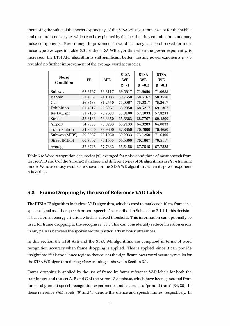
increasing the value of the power exponent p of the STSA WE algorithm, except for the babble
and restaurant noise types which can be explained by the fact that they contain non-stationary
noise components. Even though improvement in word accuracy can be observed for most
noise type averages in Table 6.6 for the STSA WE algorithm when the power exponent p is
increased, the ETSI AFE algorithm is still significant better. Testing power exponents p > 0
revealed no further improvement of the average word accuracies.
NoiseCondition
FE AFESTSAWE
p=-1
STSAWE
p=-0.3
STSAWE
p=-0.1
Subway 62.2767 79.3117 69.5617 71.6050 71.0683Babble 51.4367 74.1083 59.7550 58.6167 58.3550Car 56.8433 81.2550 71.0067 75.0817 75.2617Exhibition 61.4317 79.3267 65.2950 68.5217 69.1367Restaurant 53.7150 73.7633 57.8100 57.4033 57.8233Street 58.3133 78.3350 65.6683 68.7767 69.4800Airport 54.7233 78.9233 63.7133 64.0283 64.0833Train-Station 54.3650 79.9600 67.8650 70.2000 70.4650Subway (MIRS) 59.9067 76.1950 69.2033 73.1250 71.6400Street (MIRS) 60.7367 76.1533 65.5800 70.1867 70.5117
Average 57.3748 77.7332 65.5458 67.7545 67.7825
Table 6.6: Word recognition accuracies [%] averaged for noise conditions of noisy speech fromtest set A, B and C of the Aurora-2 database and different types of SE algorithms in clean trainingmode. Word accuracy results are shown for the STSA WE algorithm, when its power exponentp is varied.
6.3 Frame Dropping by the use of Reference VAD Labels
The ETSI AFE algorithm includes a VAD algorithm, which is used to mark each 10 ms frame in a
speech signal as either speech or non-speech. As described in Subsection 3.1.1.1, this decision
is based on an energy criterion which is a fixed threshold. This information can optionally be
used for frame dropping at the recogniser [33]. This can considerably reduce insertion errors
in any pauses between the spoken words, particularly in noisy utterances.
In this section the ETSI AFE and the STSA WE algorithms are compared in terms of word
recognition accuracy when frame dropping is applied. This is applied, since it can provide
insight into if it is the silence regions that causes the significant lower word accuracy results for
the STSA WE algorithm during clean training as shown in Section 6.1.
Frame dropping is applied by the use of frame-by-frame reference VAD labels for both the
training set and test set A, B and C of the Aurora-2 database, which have been generated from
forced-alignment speech recognition experiments and is used as a "ground truth" [34, 35]. In
these reference VAD labels, ’0’ and ’1’ denote the silence and speech frames, respectively. In
88
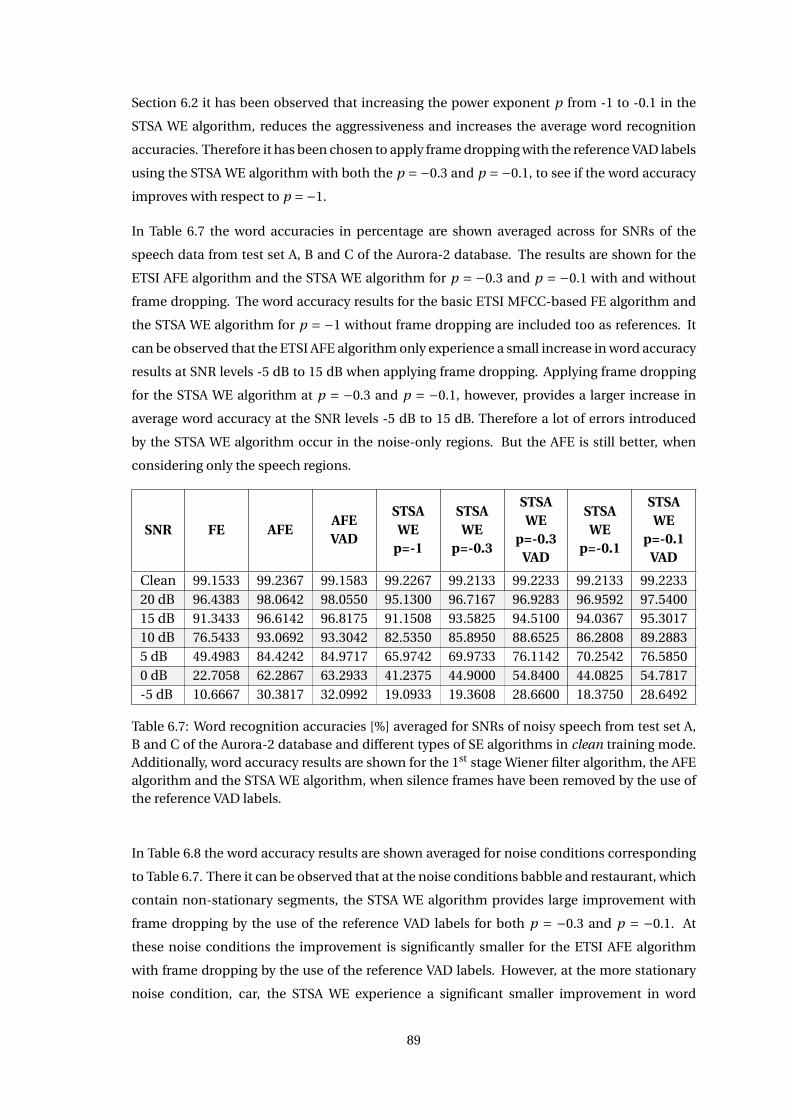
Section 6.2 it has been observed that increasing the power exponent p from -1 to -0.1 in the
STSA WE algorithm, reduces the aggressiveness and increases the average word recognition
accuracies. Therefore it has been chosen to apply frame dropping with the reference VAD labels
using the STSA WE algorithm with both the p =−0.3 and p =−0.1, to see if the word accuracy
improves with respect to p =−1.
In Table 6.7 the word accuracies in percentage are shown averaged across for SNRs of the
speech data from test set A, B and C of the Aurora-2 database. The results are shown for the
ETSI AFE algorithm and the STSA WE algorithm for p = −0.3 and p = −0.1 with and without
frame dropping. The word accuracy results for the basic ETSI MFCC-based FE algorithm and
the STSA WE algorithm for p = −1 without frame dropping are included too as references. It
can be observed that the ETSI AFE algorithm only experience a small increase in word accuracy
results at SNR levels -5 dB to 15 dB when applying frame dropping. Applying frame dropping
for the STSA WE algorithm at p = −0.3 and p = −0.1, however, provides a larger increase in
average word accuracy at the SNR levels -5 dB to 15 dB. Therefore a lot of errors introduced
by the STSA WE algorithm occur in the noise-only regions. But the AFE is still better, when
considering only the speech regions.
SNR FE AFEAFEVAD
STSAWE
p=-1
STSAWE
p=-0.3
STSAWE
p=-0.3VAD
STSAWE
p=-0.1
STSAWE
p=-0.1VAD
Clean 99.1533 99.2367 99.1583 99.2267 99.2133 99.2233 99.2133 99.223320 dB 96.4383 98.0642 98.0550 95.1300 96.7167 96.9283 96.9592 97.540015 dB 91.3433 96.6142 96.8175 91.1508 93.5825 94.5100 94.0367 95.301710 dB 76.5433 93.0692 93.3042 82.5350 85.8950 88.6525 86.2808 89.28835 dB 49.4983 84.4242 84.9717 65.9742 69.9733 76.1142 70.2542 76.58500 dB 22.7058 62.2867 63.2933 41.2375 44.9000 54.8400 44.0825 54.7817-5 dB 10.6667 30.3817 32.0992 19.0933 19.3608 28.6600 18.3750 28.6492
Table 6.7: Word recognition accuracies [%] averaged for SNRs of noisy speech from test set A,B and C of the Aurora-2 database and different types of SE algorithms in clean training mode.Additionally, word accuracy results are shown for the 1st stage Wiener filter algorithm, the AFEalgorithm and the STSA WE algorithm, when silence frames have been removed by the use ofthe reference VAD labels.
In Table 6.8 the word accuracy results are shown averaged for noise conditions corresponding
to Table 6.7. There it can be observed that at the noise conditions babble and restaurant, which
contain non-stationary segments, the STSA WE algorithm provides large improvement with
frame dropping by the use of the reference VAD labels for both p = −0.3 and p = −0.1. At
these noise conditions the improvement is significantly smaller for the ETSI AFE algorithm
with frame dropping by the use of the reference VAD labels. However, at the more stationary
noise condition, car, the STSA WE experience a significant smaller improvement in word
89
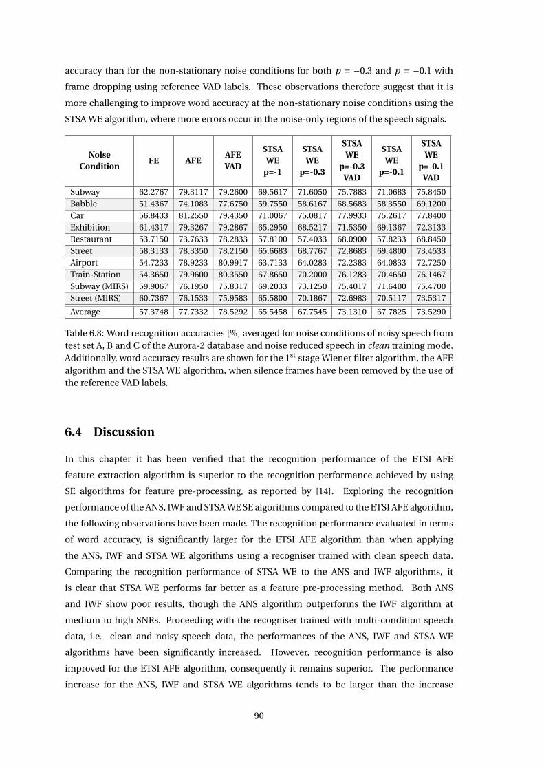
accuracy than for the non-stationary noise conditions for both p = −0.3 and p = −0.1 with
frame dropping using reference VAD labels. These observations therefore suggest that it is
more challenging to improve word accuracy at the non-stationary noise conditions using the
STSA WE algorithm, where more errors occur in the noise-only regions of the speech signals.
NoiseCondition
FE AFEAFEVAD
STSAWE
p=-1
STSAWE
p=-0.3
STSAWE
p=-0.3VAD
STSAWE
p=-0.1
STSAWE
p=-0.1VAD
Subway 62.2767 79.3117 79.2600 69.5617 71.6050 75.7883 71.0683 75.8450Babble 51.4367 74.1083 77.6750 59.7550 58.6167 68.5683 58.3550 69.1200Car 56.8433 81.2550 79.4350 71.0067 75.0817 77.9933 75.2617 77.8400Exhibition 61.4317 79.3267 79.2867 65.2950 68.5217 71.5350 69.1367 72.3133Restaurant 53.7150 73.7633 78.2833 57.8100 57.4033 68.0900 57.8233 68.8450Street 58.3133 78.3350 78.2150 65.6683 68.7767 72.8683 69.4800 73.4533Airport 54.7233 78.9233 80.9917 63.7133 64.0283 72.2383 64.0833 72.7250Train-Station 54.3650 79.9600 80.3550 67.8650 70.2000 76.1283 70.4650 76.1467Subway (MIRS) 59.9067 76.1950 75.8317 69.2033 73.1250 75.4017 71.6400 75.4700Street (MIRS) 60.7367 76.1533 75.9583 65.5800 70.1867 72.6983 70.5117 73.5317
Average 57.3748 77.7332 78.5292 65.5458 67.7545 73.1310 67.7825 73.5290
Table 6.8: Word recognition accuracies [%] averaged for noise conditions of noisy speech fromtest set A, B and C of the Aurora-2 database and noise reduced speech in clean training mode.Additionally, word accuracy results are shown for the 1st stage Wiener filter algorithm, the AFEalgorithm and the STSA WE algorithm, when silence frames have been removed by the use ofthe reference VAD labels.
6.4 Discussion
In this chapter it has been verified that the recognition performance of the ETSI AFE
feature extraction algorithm is superior to the recognition performance achieved by using
SE algorithms for feature pre-processing, as reported by [14]. Exploring the recognition
performance of the ANS, IWF and STSA WE SE algorithms compared to the ETSI AFE algorithm,
the following observations have been made. The recognition performance evaluated in terms
of word accuracy, is significantly larger for the ETSI AFE algorithm than when applying
the ANS, IWF and STSA WE algorithms using a recogniser trained with clean speech data.
Comparing the recognition performance of STSA WE to the ANS and IWF algorithms, it
is clear that STSA WE performs far better as a feature pre-processing method. Both ANS
and IWF show poor results, though the ANS algorithm outperforms the IWF algorithm at
medium to high SNRs. Proceeding with the recogniser trained with multi-condition speech
data, i.e. clean and noisy speech data, the performances of the ANS, IWF and STSA WE
algorithms have been significantly increased. However, recognition performance is also
improved for the ETSI AFE algorithm, consequently it remains superior. The performance
increase for the ANS, IWF and STSA WE algorithms tends to be larger than the increase
90
experienced by the ETSI AFE algorithm. This difference can most likely be explained by the
ETSI AFE being more robust towards noisy speech data as observed during clean training
mode. The recognition performance of the STSA WE has been increased by adjusting its power
exponent p, which has an influence on the aggressiveness of the applied noise reduction. The
most significant increase occurs for reduced aggressiveness at medium SNRs. However, the
recognition performance can suffer at low SNRs, if the aggressiveness is reduced too much.
The difference of recognition performance between STSA WE and ETSI AFE is further explored
by introducing frame dropping using reference VAD labels i.e. dropping the silence frames
from the speech signals. Frame dropping increases recognition performance of the STSA WE
algorithm regardless of the aggressiveness applied. However, the STSA WE algorithm is still
outperformed by the ETSI AFE algorithm even though frame dropping only slightly increases
the recognition performance of ETSI AFE. This means that the STSA WE algorithm is more
affected by recognition errors in the noise-only regions at low SNRs. This suggest that in order
to improve the recognition performance of the STSA WE, it might be reasonable to improve
its VAD and noise power spectrum estimation, to allow for better handling of the noise-only
regions.
91

Correlation of ASR and
Speech Enhancement
Performance Measures 7In this chapter the correlation between selected ASR performance measures and selected SE
performance measures is investigated. In [39] it has been investigated if it is possible to create
an estimator of the performance of a speech recognition system using the PESQ measure for
various noise reduction algorithms, with positive results. This chapter investigates if such a
predictor can be created for the ETSI AFE algorithm using either STOI or PESQ.
It takes a larger computational load to perform speech recognition than computing STOI
and PESQ scores for speech signals. Therefore an estimator can be used to enable more
rapid configuration during the development phases of ASR systems. It is mostly aimed at
development phases as STOI and PESQ both require an original noise free reference signal.
First, the correlation coefficients utilized are presented. These are then used to investigate
the feasibility of using denoised signals to estimate the final ASR performance using the
ETSI AFE. The denoised signals are extracted after the waveform processing block in the ETSI
AFE algorithm as shown in Figure 5.1. Next the correlation between the ASR performance
measures and SE performance measures of the ETSI AFE is explored, where it is attempted
to design an estimator of ASR performance using SE performance measures representing the
difference between a denoised speech signal and its original clean version, see Figure 7.1.
Finally the correlation between ASR performance measures and STOI/PESQ for the different
feature extraction algorithms at fixed SNR levels is explored.
93
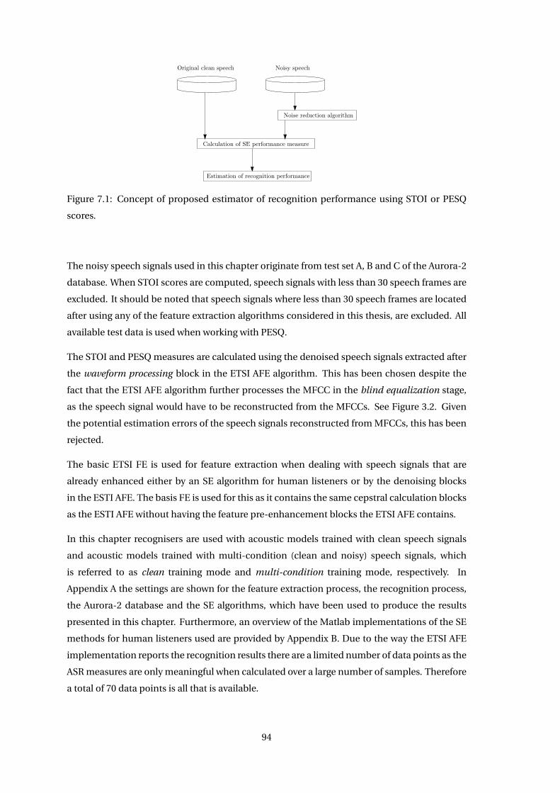
Noise reduction algorithm
Calculation of SE performance measure
Estimation of recognition performance
Original clean speech Noisy speech
Figure 7.1: Concept of proposed estimator of recognition performance using STOI or PESQ
scores.
The noisy speech signals used in this chapter originate from test set A, B and C of the Aurora-2
database. When STOI scores are computed, speech signals with less than 30 speech frames are
excluded. It should be noted that speech signals where less than 30 speech frames are located
after using any of the feature extraction algorithms considered in this thesis, are excluded. All
available test data is used when working with PESQ.
The STOI and PESQ measures are calculated using the denoised speech signals extracted after
the waveform processing block in the ETSI AFE algorithm. This has been chosen despite the
fact that the ETSI AFE algorithm further processes the MFCC in the blind equalization stage,
as the speech signal would have to be reconstructed from the MFCCs. See Figure 3.2. Given
the potential estimation errors of the speech signals reconstructed from MFCCs, this has been
rejected.
The basic ETSI FE is used for feature extraction when dealing with speech signals that are
already enhanced either by an SE algorithm for human listeners or by the denoising blocks
in the ESTI AFE. The basis FE is used for this as it contains the same cepstral calculation blocks
as the ESTI AFE without having the feature pre-enhancement blocks the ETSI AFE contains.
In this chapter recognisers are used with acoustic models trained with clean speech signals
and acoustic models trained with multi-condition (clean and noisy) speech signals, which
is referred to as clean training mode and multi-condition training mode, respectively. In
Appendix A the settings are shown for the feature extraction process, the recognition process,
the Aurora-2 database and the SE algorithms, which have been used to produce the results
presented in this chapter. Furthermore, an overview of the Matlab implementations of the SE
methods for human listeners used are provided by Appendix B. Due to the way the ETSI AFE
implementation reports the recognition results there are a limited number of data points as the
ASR measures are only meaningful when calculated over a large number of samples. Therefore
a total of 70 data points is all that is available.
94
7.1 Correlation Coefficients
In this section the correlation coefficients utilized in this chapter are presented, specifically
the Pearson correlation coefficient, the Spearman rank correlation coefficient and the Kendall
Tau rank correlation coefficient. The Pearson correlation coefficient is considered as this is
the basic linear and most commonly used correlation coefficient [2]. But we do not assume
that the relationships considered are linear. Therefore the Spearman and Kendall correlation
coefficients are additionally considered, as they measure the monotonic correlation between
two dataset and are also commonly used [2]. The value of the correlation coefficients are
within the range [-1, 1], where the magnitude of the coefficient indicates the strength of the
correlation. This mean if the correlation coefficient is 0 there is no correlation and if it is 1
there is perfect correlation, while the sign indicates if the correlation is positive or negative [2].
A description of the Pearson, the Spearman and the Kendall correlation coefficients are given
in the following subsections.
7.1.1 Pearson Correlation Coefficient
The Pearson correlation coefficient is a measure of the linear correlation between two data
sets. Two datasets of raw scores, x = [x1x2 · · ·xN ]T and y = [y1 y2 · · · yN ]T, are considered and are
linear transformed into standardizes z-scores, zxi and zyi for i = 1, ..., N . Each member i of the
set of raw scores x is linear transformed by the use of the following equation:
zxi =xi − x
sx, (7.1)
where x is the mean and sx is the standard deviation of x given by:
x = 1
N
N∑i=1
xi , (7.2)
sx =√√√√ 1
N −1
N∑i=1
(xi − x)2. (7.3)
The z-score representing a raw score can be interpreted as the number of standard deviations
the raw score is above or below the mean of the distribution. The mean of a complete set of
z-scores is zero and both the standard deviation and the variance have a value of 1 [24]. The
Pearson correlation coefficient for the two datasets x and y is then given by:
rx y = 1
N −1
N∑i=1
zxi zyi . (7.4)
This correlation coefficient is basically the average of the dot product of the z-scores of x and y.
rx y can be interpreted as a measure of how similar zxi is to zyi on average. If there is a perfect
positive correlation between x and y, then zyi = zxi for i = 1, ..., N , so the correlation is
rx y = 1
N −1
N∑i=1
zxi zyi =1
N −1
N∑i=1
z2xi= 1. (7.5)
95
If there is a perfect negative correlation, zyi =−zxi for i = 1, ..., N , then rx y =−1 [24]. Equation
7.4 can also be reformulated as the covariance between x and y, normalized by the product of
the standard deviations of x and y:
rx y =
N∑i=1
(xi − x)(yi − y)√√√√ N∑i=1
(xi − x)2
√√√√ N∑i=1
(yi − y)2
. (7.6)
This equation can be thought of as an expression of a ratio of how much x and y vary together
compared to how much x and y vary separately [2]. In summary, the Pearson correlation
coefficient is a numerical measure of the degree to which x and y are linearly related [24].
7.1.2 Spearman Rank Correlation Coefficient
The Spearman rank correlation coefficient is obtained by the use of the Pearson correlation
coefficient. Spearman assess the monotonic relationship function between two datasets x =[x1x2 · · ·xN ]T and y = [y1 y2 · · · yN ]T, where a function is said to be monotonic if it is either
entirely increasing or decreasing [24].
The raw data is converted into ranking variables. The Spearman correlation coefficient is
obtained by applying Pearson on the ranked data. Ranking variables are found by assigning
rank 1 to the smallest raw value and rank N to the largest raw value. If there are tied values, all
the ranking scores in a group of ties are given the mean of the ranks they would have received
had there been no ties. For example, if four scores are tied for the 10th place after the nine
largest scores have been ranked, each receives the rank 11.5 (mean of 10, 11, 12 and 13). The
next largest score receives a rank of 14 [24].
There exists a simplified expression for computing the Spearman rank correlation coefficient,
which takes advantage of the characteristics of ranks. This assumes that no ties exists,
therefore the mean and the variance of a set of N ranks are given by (N + 1)/2 and
N (N + 1)/12, respectively [24]. Substituting these expressions into the Pearson correlation
coefficient formula, given by Equation 7.6, yields the following expression of the Spearman
rank correlation coefficient [24]:
rs = 1− 6∑N
i=1 d 2i
N (N 2 −1), (7.7)
where di is the difference between ranks for the i th case. Equation 7.7 only applies if there are
no tied ranks as the variance gets reduced when ties are present.
Finally an example of the computation of the Spearman rank correlation coefficient is
provided. In Table 7.1 raw data for x and y are presented with their corresponding rankings
and the squared difference between the rankings d 2i for the i th case.
96
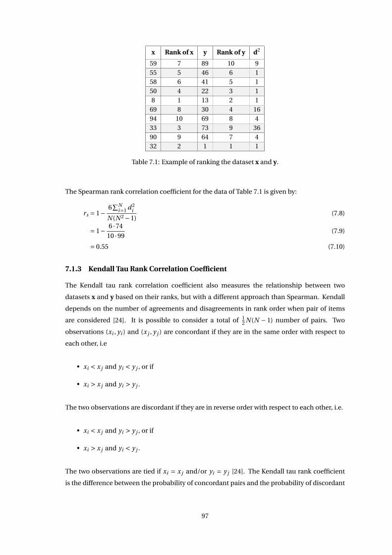
x Rank of x y Rank of y d2
59 7 89 10 955 5 46 6 158 6 41 5 150 4 22 3 18 1 13 2 1
69 8 30 4 1694 10 69 8 433 3 73 9 3690 9 64 7 432 2 1 1 1
Table 7.1: Example of ranking the dataset x and y.
The Spearman rank correlation coefficient for the data of Table 7.1 is given by:
rs = 1− 6∑N
i=1 d 2i
N (N 2 −1)(7.8)
= 1− 6 ·74
10 ·99(7.9)
= 0.55 (7.10)
7.1.3 Kendall Tau Rank Correlation Coefficient
The Kendall tau rank correlation coefficient also measures the relationship between two
datasets x and y based on their ranks, but with a different approach than Spearman. Kendall
depends on the number of agreements and disagreements in rank order when pair of items
are considered [24]. It is possible to consider a total of 12 N (N − 1) number of pairs. Two
observations (xi , yi ) and (x j , y j ) are concordant if they are in the same order with respect to
each other, i.e
• xi < x j and yi < y j , or if
• xi > x j and yi > y j .
The two observations are discordant if they are in reverse order with respect to each other, i.e.
• xi < x j and yi > y j , or if
• xi > x j and yi < y j .
The two observations are tied if xi = x j and/or yi = y j [24]. The Kendall tau rank coefficient
is the difference between the probability of concordant pairs and the probability of discordant
97
pairs:
τ= (number of concordant pairs)− (number of discordant pairs)12 N (N −1)
, (7.11)
where N is the number of observations in each data set and the denominator is the total
number of pairs. Equation 7.11 is only valid when there are no tied ranks [24].
7.2 Impact of Blind Equalization on Correlation Between
STOI/PESQ Scores and ASR Results
This section investigates the correlation between the STOI/PESQ scores of denoised speech
signals and the corresponding ASR measures obtained using the ETSI AFE feature extraction
algorithm. The denoised signals are extracted after the waveform processing block of the ETSI
AFE algorithm as shown in Figure 5.1. But the ETSI AFE algorithm includes an additional blind
equalization block operating in the cepstral domain in order for the ASR system to be robust
against channel variations as described in Section 3.1. In order for the correlation results
obtained using the ETSI AFE algorithm to be comparable to other algorithms, the impact of
the blind equalization block on the correlation results has to be ignored. If the impact is
negligible, then the comparison is fair. The impact of the blind equalization block is then
evaluated by comparing correlation coefficients when ASR results are obtained for feature
extraction with and without blind equalization. ASR results without blind equalization are
obtained by applying the basic ETSI MFCC-based FE on the denoised speech signals extracted
after the waveform processing block in the ETSI AFE algorithm (denoted by WFP-FE). It should
be noted that the contribution of the blind equalization block on ASR performance can be seen
in Section 6.1 by comparing the performance of the extracted waveform processing speech
signals to the AFE.
Table 7.2 shows the Pearson, Spearman and Kendall correlation coefficients between the
word accuracies (using the feature extraction methods (AFE and WFP-FE) in ASR) and the
corresponding STOI/PESQ scores for the denoised speech signals. Furthermore, correlation
coefficients are calculated over all data i.e. combining the data for feature extraction with and
without blind equalization. Both clean and multi-condition training modes are considered.
It has been chosen to consider only the word accuracy of the available ASR performance
measures, as it accounts for all kinds of errors appearing in ASR unlike word correct and the
fact that each error is weighted equally unlike the sentence correct performance measure.
98
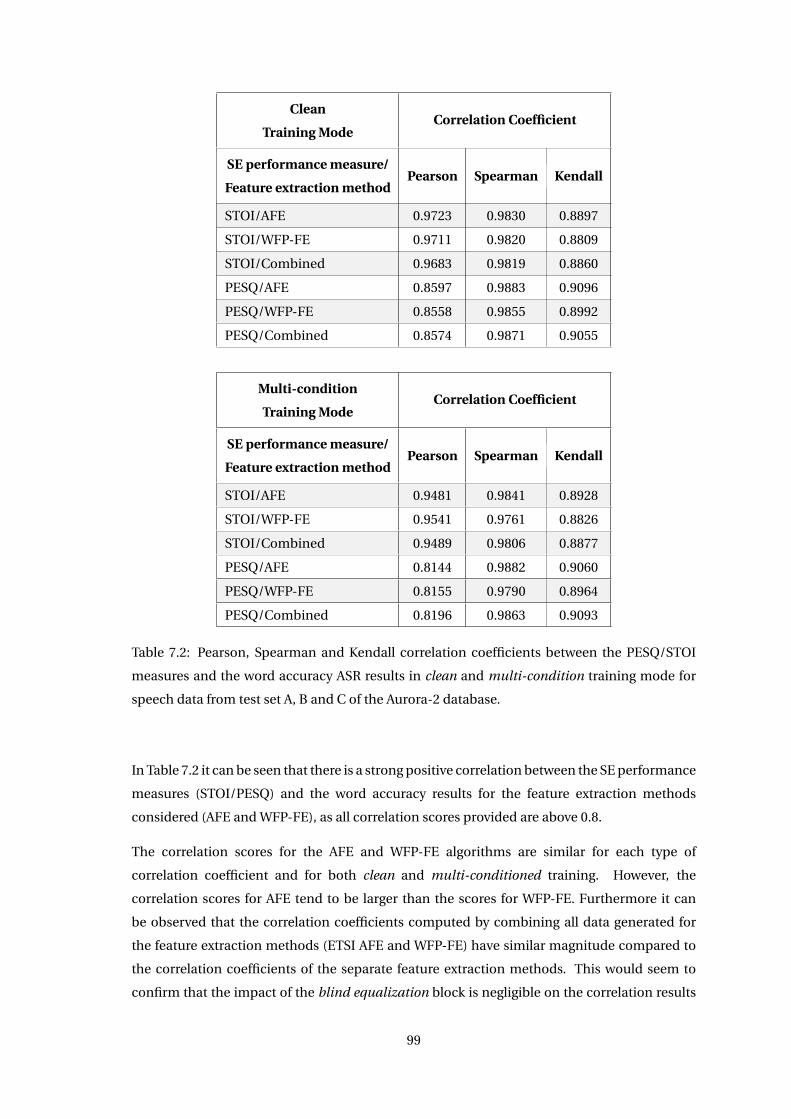
Clean
Training ModeCorrelation Coefficient
SE performance measure/
Feature extraction methodPearson Spearman Kendall
STOI/AFE 0.9723 0.9830 0.8897
STOI/WFP-FE 0.9711 0.9820 0.8809
STOI/Combined 0.9683 0.9819 0.8860
PESQ/AFE 0.8597 0.9883 0.9096
PESQ/WFP-FE 0.8558 0.9855 0.8992
PESQ/Combined 0.8574 0.9871 0.9055
Multi-condition
Training ModeCorrelation Coefficient
SE performance measure/
Feature extraction methodPearson Spearman Kendall
STOI/AFE 0.9481 0.9841 0.8928
STOI/WFP-FE 0.9541 0.9761 0.8826
STOI/Combined 0.9489 0.9806 0.8877
PESQ/AFE 0.8144 0.9882 0.9060
PESQ/WFP-FE 0.8155 0.9790 0.8964
PESQ/Combined 0.8196 0.9863 0.9093
Table 7.2: Pearson, Spearman and Kendall correlation coefficients between the PESQ/STOI
measures and the word accuracy ASR results in clean and multi-condition training mode for
speech data from test set A, B and C of the Aurora-2 database.
In Table 7.2 it can be seen that there is a strong positive correlation between the SE performance
measures (STOI/PESQ) and the word accuracy results for the feature extraction methods
considered (AFE and WFP-FE), as all correlation scores provided are above 0.8.
The correlation scores for the AFE and WFP-FE algorithms are similar for each type of
correlation coefficient and for both clean and multi-conditioned training. However, the
correlation scores for AFE tend to be larger than the scores for WFP-FE. Furthermore it can
be observed that the correlation coefficients computed by combining all data generated for
the feature extraction methods (ETSI AFE and WFP-FE) have similar magnitude compared to
the correlation coefficients of the separate feature extraction methods. This would seem to
confirm that the impact of the blind equalization block is negligible on the correlation results
99
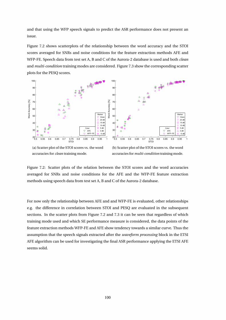
and that using the WFP speech signals to predict the ASR performance does not present an
issue.
Figure 7.2 shows scatterplots of the relationship between the word accuracy and the STOI
scores averaged for SNRs and noise conditions for the feature extraction methods AFE and
WFP-FE. Speech data from test set A, B and C of the Aurora-2 database is used and both clean
and multi-condition training modes are considered. Figure 7.3 show the corresponding scatter
plots for the PESQ scores.
0.5 0.55 0.6 0.65 0.7 0.75 0.8 0.85 0.9 0.95 120
30
40
50
60
70
80
90
100
STOI
Wor
dnA
ccur
acyn
[E]
n
Clean
20ndB
15ndB
10ndB
5ndB
0ndB
−5ndB
Marker
AFE
WFP−FE
Color
(a) Scatter plot of the STOI scores vs. the word
accuracies for clean training mode.
0.5 0.55 0.6 0.65 0.7 0.75 0.8 0.85 0.9 0.95 120
30
40
50
60
70
80
90
100
STOI
Wor
dnA
ccur
acyn
[E]
n
Clean
20ndB
15ndB
10ndB
5ndB
0ndB
−5ndB
Marker
AFE
WFP−FE
Color
(b) Scatter plot of the STOI scores vs. the word
accuracies for multi-condition training mode.
Figure 7.2: Scatter plots of the relation between the STOI scores and the word accuracies
averaged for SNRs and noise conditions for the AFE and the WFP-FE feature extraction
methods using speech data from test set A, B and C of the Aurora-2 database.
For now only the relationship between AFE and and WFP-FE is evaluated, other relationships
e.g. the difference in correlation between STOI and PESQ are evaluated in the subsequent
sections. In the scatter plots from Figure 7.2 and 7.3 it can be seen that regardless of which
training mode used and which SE performance measure is considered, the data points of the
feature extraction methods WFP-FE and AFE show tendency towards a similar curve. Thus the
assumption that the speech signals extracted after the waveform processing block in the ETSI
AFE algorithm can be used for investigating the final ASR performance applying the ETSI AFE
seems solid.
100
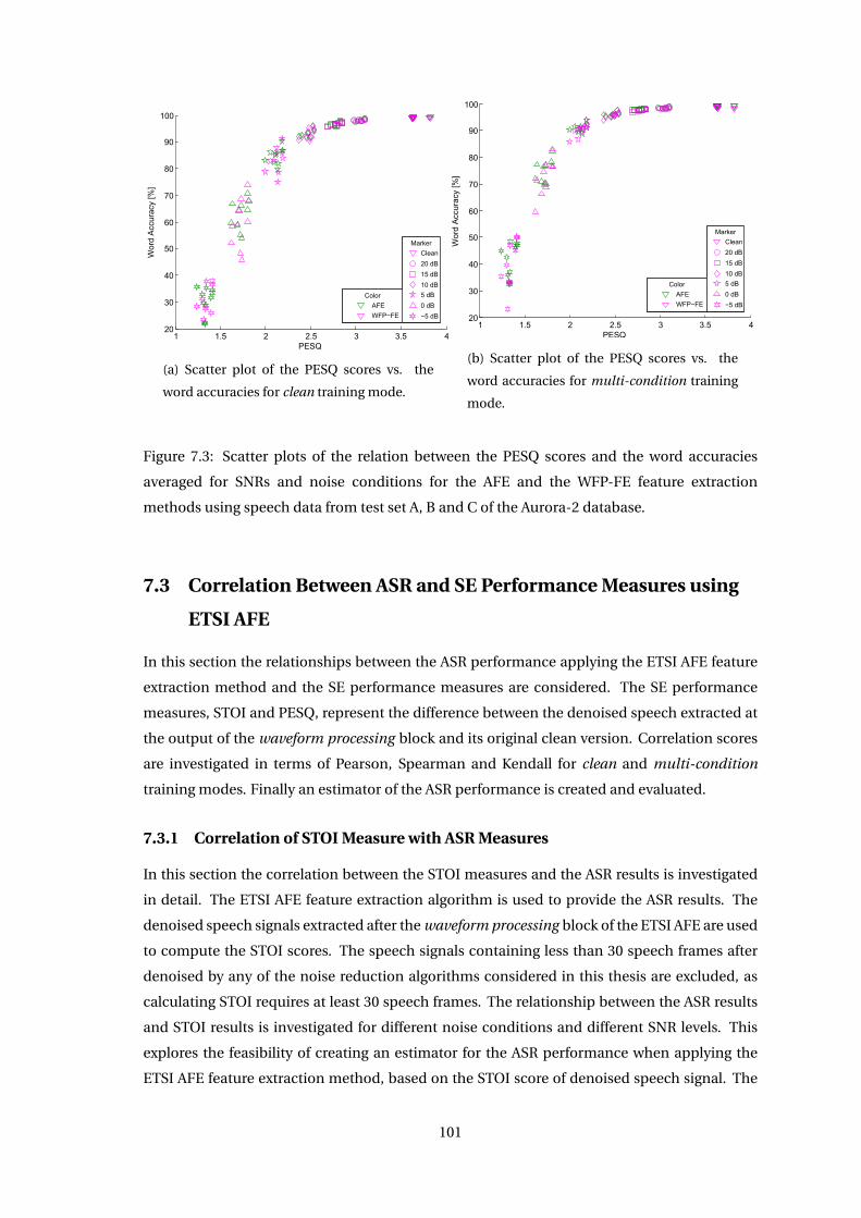
1 1.5 2 2.5 3 3.5 420
30
40
50
60
70
80
90
100
PESQ
Wor
dnA
ccur
acyn
[%]
n
Clean
20ndB
15ndB
10ndB
5ndB
0ndB
−5ndB
Marker
AFE
WFP−FE
Color
(a) Scatter plot of the PESQ scores vs. the
word accuracies for clean training mode.
1 1.5 2 2.5 3 3.5 420
30
40
50
60
70
80
90
100
PESQ
Wor
dnA
ccur
acyn
[%]
n
Clean
20ndB
15ndB
10ndB
5ndB
0ndB
−5ndB
Marker
AFE
WFP−FE
Color
(b) Scatter plot of the PESQ scores vs. the
word accuracies for multi-condition training
mode.
Figure 7.3: Scatter plots of the relation between the PESQ scores and the word accuracies
averaged for SNRs and noise conditions for the AFE and the WFP-FE feature extraction
methods using speech data from test set A, B and C of the Aurora-2 database.
7.3 Correlation Between ASR and SE Performance Measures using
ETSI AFE
In this section the relationships between the ASR performance applying the ETSI AFE feature
extraction method and the SE performance measures are considered. The SE performance
measures, STOI and PESQ, represent the difference between the denoised speech extracted at
the output of the waveform processing block and its original clean version. Correlation scores
are investigated in terms of Pearson, Spearman and Kendall for clean and multi-condition
training modes. Finally an estimator of the ASR performance is created and evaluated.
7.3.1 Correlation of STOI Measure with ASR Measures
In this section the correlation between the STOI measures and the ASR results is investigated
in detail. The ETSI AFE feature extraction algorithm is used to provide the ASR results. The
denoised speech signals extracted after the waveform processing block of the ETSI AFE are used
to compute the STOI scores. The speech signals containing less than 30 speech frames after
denoised by any of the noise reduction algorithms considered in this thesis are excluded, as
calculating STOI requires at least 30 speech frames. The relationship between the ASR results
and STOI results is investigated for different noise conditions and different SNR levels. This
explores the feasibility of creating an estimator for the ASR performance when applying the
ETSI AFE feature extraction method, based on the STOI score of denoised speech signal. The
101
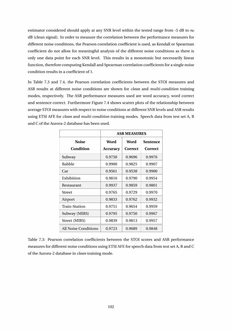
estimator considered should apply at any SNR level within the tested range from -5 dB to ∞dB (clean signal). In order to measure the correlation between the performance measures for
different noise conditions, the Pearson correlation coefficient is used, as Kendall or Spearman
coefficient do not allow for meaningful analysis of the different noise conditions as there is
only one data point for each SNR level. This results in a monotonic but necessarily linear
function, therefore computing Kendall and Spearman correlation coefficients for a single noise
condition results in a coefficient of 1.
In Table 7.3 and 7.4, the Pearson correlation coefficients between the STOI measures and
ASR results at different noise conditions are shown for clean and multi-condition training
modes, respectively. The ASR performance measures used are word accuracy, word correct
and sentence correct. Furthermore Figure 7.4 shows scatter plots of the relationship between
average STOI measures with respect to noise conditions at different SNR levels and ASR results
using ETSI AFE for clean and multi-condition training modes. Speech data from test set A, B
and C of the Aurora-2 database has been used.
ASR MEASURES
Noise
Condition
Word
Accuracy
Word
Correct
Sentence
Correct
Subway 0.9750 0.9696 0.9976
Babble 0.9900 0.9825 0.9907
Car 0.9561 0.9538 0.9900
Exhibition 0.9816 0.9790 0.9954
Restaurant 0.9937 0.9859 0.9801
Street 0.9765 0.9729 0.9970
Airport 0.9833 0.9762 0.9932
Train-Station 0.9751 0.9654 0.9959
Subway (MIRS) 0.9795 0.9750 0.9967
Street (MIRS) 0.9839 0.9813 0.9957
All Noise Conditions 0.9723 0.9689 0.9848
Table 7.3: Pearson correlation coefficients between the STOI scores and ASR performance
measures for different noise conditions using ETSI AFE for speech data from test set A, B and C
of the Aurora-2 database in clean training mode.
102
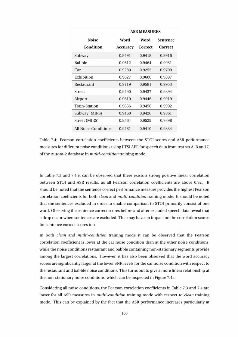
ASR MEASURES
Noise
Condition
Word
Accuracy
Word
Correct
Sentence
Correct
Subway 0.9491 0.9418 0.9916
Babble 0.9612 0.9464 0.9931
Car 0.9280 0.9255 0.9709
Exhibition 0.9627 0.9600 0.9897
Restaurant 0.9719 0.9581 0.9953
Street 0.9490 0.9437 0.9894
Airport 0.9610 0.9446 0.9919
Train-Station 0.9636 0.9456 0.9902
Subway (MIRS) 0.9460 0.9426 0.9861
Street (MIRS) 0.9564 0.9529 0.9898
All Noise Conditions 0.9481 0.9410 0.9834
Table 7.4: Pearson correlation coefficients between the STOI scores and ASR performance
measures for different noise conditions using ETSI AFE for speech data from test set A, B and C
of the Aurora-2 database in multi-condition training mode.
In Table 7.3 and 7.4 it can be observed that there exists a strong positive linear correlation
between STOI and ASR results, as all Pearson correlation coefficients are above 0.92. It
should be noted that the sentence correct performance measure provides the highest Pearson
correlation coefficients for both clean and multi-condition training mode. It should be noted
that the sentences excluded in order to enable comparison to STOI primarily consist of one
word. Observing the sentence correct scores before and after excluded speech data reveal that
a drop occur when sentences are excluded. This may have an impact on the correlation scores
for sentence correct scores too.
In both clean and multi-condition training mode it can be observed that the Pearson
correlation coefficient is lower at the car noise condition than at the other noise conditions,
while the noise conditions restaurant and babble containing non-stationary segments provide
among the largest correlations. However, it has also been observed that the word accuracy
scores are significantly larger at the lower SNR levels for the car noise condition with respect to
the restaurant and babble noise conditions. This turns out to give a more linear relationship at
the non-stationary noise conditions, which can be inspected in Figure 7.4a.
Considering all noise conditions, the Pearson correlation coefficients in Table 7.3 and 7.4 are
lower for all ASR measures in multi-condition training mode with respect to clean training
mode. This can be explained by the fact that the ASR performance increases particularly at
103
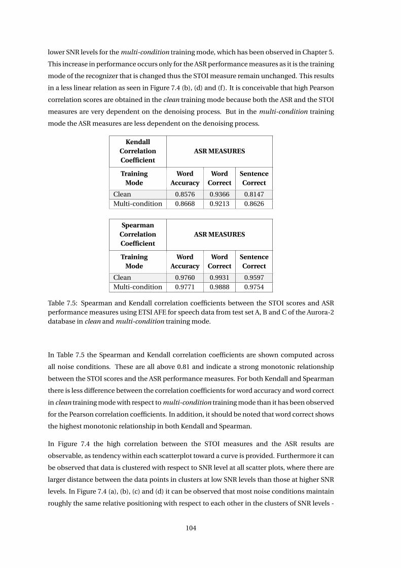
lower SNR levels for the multi-condition training mode, which has been observed in Chapter 5.
This increase in performance occurs only for the ASR performance measures as it is the training
mode of the recognizer that is changed thus the STOI measure remain unchanged. This results
in a less linear relation as seen in Figure 7.4 (b), (d) and (f). It is conceivable that high Pearson
correlation scores are obtained in the clean training mode because both the ASR and the STOI
measures are very dependent on the denoising process. But in the multi-condition training
mode the ASR measures are less dependent on the denoising process.
KendallCorrelationCoefficient
ASR MEASURES
TrainingMode
WordAccuracy
WordCorrect
SentenceCorrect
Clean 0.8576 0.9366 0.8147Multi-condition 0.8668 0.9213 0.8626
SpearmanCorrelationCoefficient
ASR MEASURES
TrainingMode
WordAccuracy
WordCorrect
SentenceCorrect
Clean 0.9760 0.9931 0.9597Multi-condition 0.9771 0.9888 0.9754
Table 7.5: Spearman and Kendall correlation coefficients between the STOI scores and ASRperformance measures using ETSI AFE for speech data from test set A, B and C of the Aurora-2database in clean and multi-condition training mode.
In Table 7.5 the Spearman and Kendall correlation coefficients are shown computed across
all noise conditions. These are all above 0.81 and indicate a strong monotonic relationship
between the STOI scores and the ASR performance measures. For both Kendall and Spearman
there is less difference between the correlation coefficients for word accuracy and word correct
in clean training mode with respect to multi-condition training mode than it has been observed
for the Pearson correlation coefficients. In addition, it should be noted that word correct shows
the highest monotonic relationship in both Kendall and Spearman.
In Figure 7.4 the high correlation between the STOI measures and the ASR results are
observable, as tendency within each scatterplot toward a curve is provided. Furthermore it can
be observed that data is clustered with respect to SNR level at all scatter plots, where there are
larger distance between the data points in clusters at low SNR levels than those at higher SNR
levels. In Figure 7.4 (a), (b), (c) and (d) it can be observed that most noise conditions maintain
roughly the same relative positioning with respect to each other in the clusters of SNR levels -
104
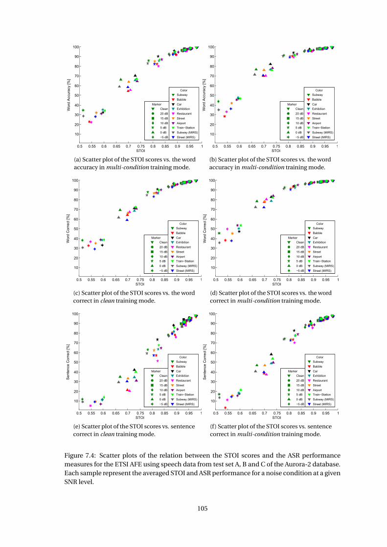
0)5 0)55 0)6 0)65 0)7 0)75 0)8 0)85 0)9 0)95 1
10
20
30
40
50
60
70
80
90
100
STOI
Wor
dlA
ccur
acyl
[h]
l
Subway
Babble
Car
Exhibition
Restaurant
Street
Airport
Train−Station
SubwaylnMIRSR
StreetlnMIRSR
Color
Clean
20ldB
15ldB
10ldB
5ldB
0ldB
−5ldB
Marker
(a) Scatter plot of the STOI scores vs. the wordaccuracy in multi-condition training mode.
0)5 0)55 0)6 0)65 0)7 0)75 0)8 0)85 0)9 0)95 1
10
20
30
40
50
60
70
80
90
100
STOI
Wor
dlA
ccur
acyl
[h]
l
Subway
Babble
Car
Exhibition
Restaurant
Street
Airport
Train−Station
SubwaylnMIRSR
StreetlnMIRSR
Color
Clean
20ldB
15ldB
10ldB
5ldB
0ldB
−5ldB
Marker
(b) Scatter plot of the STOI scores vs. the wordaccuracy in multi-condition training mode.
0)5 0)55 0)6 0)65 0)7 0)75 0)8 0)85 0)9 0)95 1
10
20
30
40
50
60
70
80
90
100
STOI
Wor
dyC
orre
cty[h
]
y
Subway
Babble
Car
Exhibition
Restaurant
Street
Airport
Train−Station
SubwayyRMIRSs
StreetyRMIRSs
Color
Clean
20ydB
15ydB
10ydB
5ydB
0ydB
−5ydB
Marker
(c) Scatter plot of the STOI scores vs. the wordcorrect in clean training mode.
0)5 0)55 0)6 0)65 0)7 0)75 0)8 0)85 0)9 0)95 1
10
20
30
40
50
60
70
80
90
100
STOI
Wor
dyC
orre
cty[h
]
y
Subway
Babble
Car
Exhibition
Restaurant
Street
Airport
Train−Station
SubwayyRMIRSs
StreetyRMIRSs
Color
Clean
20ydB
15ydB
10ydB
5ydB
0ydB
−5ydB
Marker
(d) Scatter plot of the STOI scores vs. the wordcorrect in multi-condition training mode.
0k5 0k55 0k6 0k65 0k7 0k75 0k8 0k85 0k9 0k95 1
10
20
30
40
50
60
70
80
90
100
STOI
Sen
tenc
eBC
orre
ctB[i
]
B
Subway
Babble
Car
Exhibition
Restaurant
Street
Airport
Train−Station
SubwayBAMIRSp
StreetBAMIRSp
Color
Clean
20BdB
15BdB
10BdB
5BdB
0BdB
−5BdB
Marker
(e) Scatter plot of the STOI scores vs. sentencecorrect in clean training mode.
0k5 0k55 0k6 0k65 0k7 0k75 0k8 0k85 0k9 0k95 1
10
20
30
40
50
60
70
80
90
100
STOI
Sen
tenc
eBC
orre
ctB[i
]
B
Subway
Babble
Car
Exhibition
Restaurant
Street
Airport
Train−Station
SubwayBAMIRSp
StreetBAMIRSp
Color
Clean
20BdB
15BdB
10BdB
5BdB
0BdB
−5BdB
Marker
(f) Scatter plot of the STOI scores vs. sentencecorrect in multi-condition training mode.
Figure 7.4: Scatter plots of the relation between the STOI scores and the ASR performancemeasures for the ETSI AFE using speech data from test set A, B and C of the Aurora-2 database.Each sample represent the averaged STOI and ASR performance for a noise condition at a givenSNR level.
105
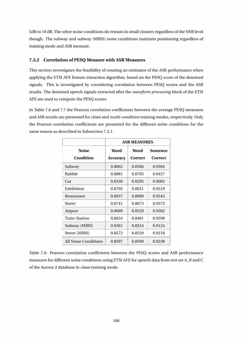
5dB to 10 dB. The other noise conditions do remain in small clusters regardless of the SNR level
though. The subway and subway (MIRS) noise conditions maintain positioning regardless of
training mode and ASR measure.
7.3.2 Correlation of PESQ Measure with ASR Measures
This section investigates the feasibility of creating an estimator of the ASR performance when
applying the ETSI AFE feature extraction algorithm, based on the PESQ score of the denoised
signals. This is investigated by considering correlation between PESQ scores and the ASR
results. The denoised speech signals extracted after the waveform processing block of the ETSI
AFE are used to compute the PESQ scores.
In Table 7.6 and 7.7 the Pearson correlation coefficients between the average PESQ measures
and ASR results are presented for clean and multi-condition training modes, respectively. Only
the Pearson correlation coefficients are presented for the different noise conditions for the
same reason as described in Subsection 7.3.1.
ASR MEASURES
Noise
Condition
Word
Accuracy
Word
Correct
Sentence
Correct
Subway 0.8662 0.8566 0.9384
Babble 0.8881 0.8705 0.9427
Car 0.8330 0.8295 0.9005
Exhibition 0.8705 0.8651 0.9319
Restaurant 0.8937 0.8689 0.9543
Street 0.8741 0.8673 0.9373
Airport 0.8689 0.8520 0.9302
Train-Station 0.8654 0.8481 0.9290
Subway (MIRS) 0.8361 0.8254 0.9124
Street (MIRS) 0.8572 0.8529 0.9218
All Noise Conditions 0.8597 0.8509 0.9238
Table 7.6: Pearson correlation coefficients between the PESQ scores and ASR performance
measures for different noise conditions using ETSI AFE for speech data from test set A, B and C
of the Aurora-2 database in clean training mode.
106
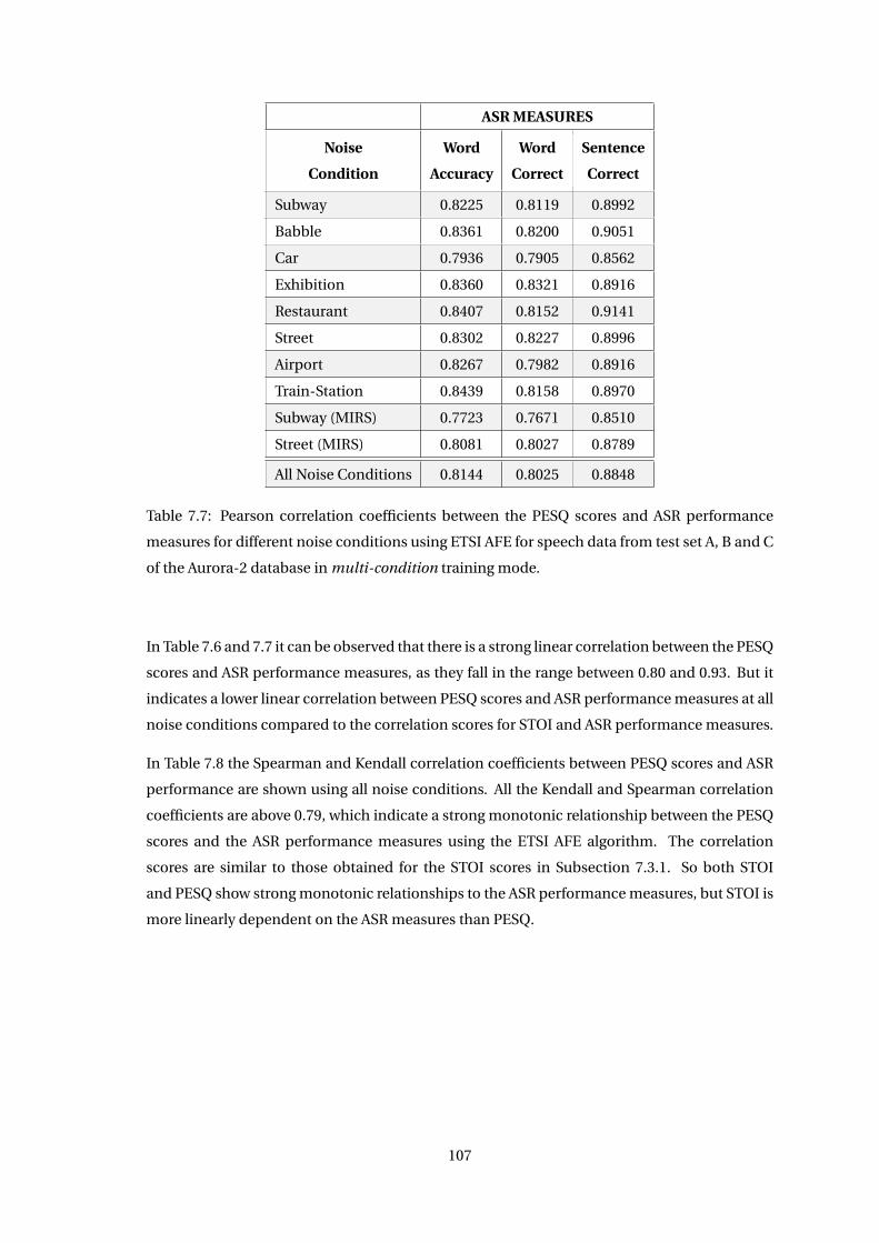
ASR MEASURES
Noise
Condition
Word
Accuracy
Word
Correct
Sentence
Correct
Subway 0.8225 0.8119 0.8992
Babble 0.8361 0.8200 0.9051
Car 0.7936 0.7905 0.8562
Exhibition 0.8360 0.8321 0.8916
Restaurant 0.8407 0.8152 0.9141
Street 0.8302 0.8227 0.8996
Airport 0.8267 0.7982 0.8916
Train-Station 0.8439 0.8158 0.8970
Subway (MIRS) 0.7723 0.7671 0.8510
Street (MIRS) 0.8081 0.8027 0.8789
All Noise Conditions 0.8144 0.8025 0.8848
Table 7.7: Pearson correlation coefficients between the PESQ scores and ASR performance
measures for different noise conditions using ETSI AFE for speech data from test set A, B and C
of the Aurora-2 database in multi-condition training mode.
In Table 7.6 and 7.7 it can be observed that there is a strong linear correlation between the PESQ
scores and ASR performance measures, as they fall in the range between 0.80 and 0.93. But it
indicates a lower linear correlation between PESQ scores and ASR performance measures at all
noise conditions compared to the correlation scores for STOI and ASR performance measures.
In Table 7.8 the Spearman and Kendall correlation coefficients between PESQ scores and ASR
performance are shown using all noise conditions. All the Kendall and Spearman correlation
coefficients are above 0.79, which indicate a strong monotonic relationship between the PESQ
scores and the ASR performance measures using the ETSI AFE algorithm. The correlation
scores are similar to those obtained for the STOI scores in Subsection 7.3.1. So both STOI
and PESQ show strong monotonic relationships to the ASR performance measures, but STOI is
more linearly dependent on the ASR measures than PESQ.
107
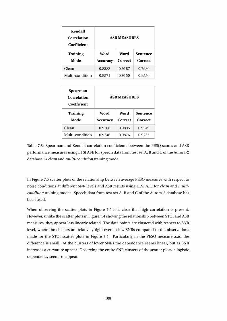
Kendall
Correlation
Coefficient
ASR MEASURES
Training
Mode
Word
Accuracy
Word
Correct
Sentence
Correct
Clean 0.8283 0.9187 0.7980
Multi-condition 0.8571 0.9150 0.8550
Spearman
Correlation
Coefficient
ASR MEASURES
Training
Mode
Word
Accuracy
Word
Correct
Sentence
Correct
Clean 0.9706 0.9895 0.9549
Multi-condition 0.9746 0.9876 0.9735
Table 7.8: Spearman and Kendall correlation coefficients between the PESQ scores and ASR
performance measures using ETSI AFE for speech data from test set A, B and C of the Aurora-2
database in clean and multi-condition training mode.
In Figure 7.5 scatter plots of the relationship between average PESQ measures with respect to
noise conditions at different SNR levels and ASR results using ETSI AFE for clean and multi-
condition training modes. Speech data from test set A, B and C of the Aurora-2 database has
been used.
When observing the scatter plots in Figure 7.5 it is clear that high correlation is present.
However, unlike the scatter plots in Figure 7.4 showing the relationship between STOI and ASR
measures, they appear less linearly related. The data points are clustered with respect to SNR
level, where the clusters are relatively tight even at low SNRs compared to the observations
made for the STOI scatter plots in Figure 7.4. Particularly in the PESQ measure axis, the
difference is small. At the clusters of lower SNRs the dependence seems linear, but as SNR
increases a curvature appear. Observing the entire SNR clusters of the scatter plots, a logistic
dependency seems to appear.
108
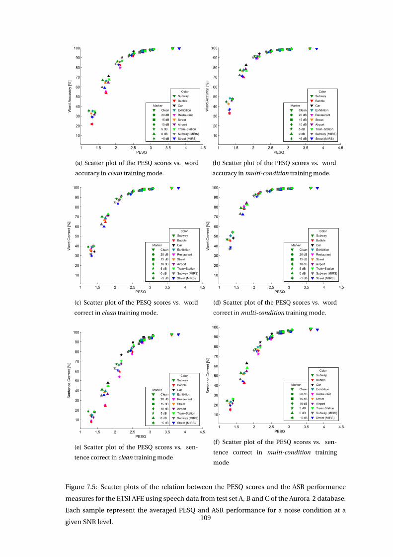
1 1I5 2 2I5 3 3I5 4 4I5
1k
2k
3k
4k
5k
6k
7k
8k
9k
1kk
PESQ
Wor
dlA
ccur
acyl
[i]
l
Subway
Babble
Car
Exhibition
Restaurant
Street
Airport
Train−Station
SubwaylRMIRSs
StreetlRMIRSs
Color
Clean
2kldB
15ldB
1kldB
5ldB
kldB
−5ldB
Marker
(a) Scatter plot of the PESQ scores vs. word
accuracy in clean training mode.
1 1I5 2 2I5 3 3I5 4 4I5
1k
2k
3k
4k
5k
6k
7k
8k
9k
1kk
PESQ
Wor
dlA
ccur
cyl[i
]
l
Subway
Babble
Car
Exhibition
Restaurant
Street
Airport
Train−Station
SubwaylRMIRSs
StreetlRMIRSs
Color
Clean
2kldB
15ldB
1kldB
5ldB
kldB
−5ldB
Marker
(b) Scatter plot of the PESQ scores vs. word
accuracy in multi-condition training mode.
1 1I5 2 2I5 3 3I5 4 4I5
1k
2k
3k
4k
5k
6k
7k
8k
9k
1kk
PESQ
Wor
dyC
orre
cty[i
]
y
Subway
Babble
Car
Exhibition
Restaurant
Street
Airport
Train−Station
SubwayysMIRSA
StreetysMIRSA
Color
Clean
2kydB
15ydB
1kydB
5ydB
kydB
−5ydB
Marker
(c) Scatter plot of the PESQ scores vs. word
correct in clean training mode.
1 1I5 2 2I5 3 3I5 4 4I5
1k
2k
3k
4k
5k
6k
7k
8k
9k
1kk
PESQ
Wor
dyC
orre
cty[i
]
y
Subway
Babble
Car
Exhibition
Restaurant
Street
Airport
Train−Station
SubwayysMIRSA
StreetysMIRSA
Color
Clean
2kydB
15ydB
1kydB
5ydB
kydB
−5ydB
Marker
(d) Scatter plot of the PESQ scores vs. word
correct in multi-condition training mode.
1 1d5 2 2d5 3 3d5 4 4d5
10
20
30
40
50
60
70
80
90
100
PESQ
Sen
tenc
eBC
orre
ctB[R
]
B
Subway
Babble
Car
Exhibition
Restaurant
Street
Airport
Train−Station
SubwayBpMIRST
StreetBpMIRST
Color
Clean
20BdB
15BdB
10BdB
5BdB
0BdB
−5BdB
Marker
(e) Scatter plot of the PESQ scores vs. sen-
tence correct in clean training mode
1 1d5 2 2d5 3 3d5 4 4d5
10
20
30
40
50
60
70
80
90
100
PESQ
Sen
tenc
eBC
orre
ctB[R
]
B
Subway
Babble
Car
Exhibition
Restaurant
Street
Airport
Train−Station
SubwayBpMIRST
StreetBpMIRST
Color
Clean
20BdB
15BdB
10BdB
5BdB
0BdB
−5BdB
Marker
(f) Scatter plot of the PESQ scores vs. sen-
tence correct in multi-condition training
mode
Figure 7.5: Scatter plots of the relation between the PESQ scores and the ASR performance
measures for the ETSI AFE using speech data from test set A, B and C of the Aurora-2 database.
Each sample represent the averaged PESQ and ASR performance for a noise condition at a
given SNR level.109
7.3.3 Estimation of the ETSI AFE Recognition Performance
In Subsection 7.3.1 and 7.3.2 it has been observed that a strong monotonic relationship exist
between STOI/PESQ and the ASR performance measures when applying the ETSI AFE feature
extraction algorithm. The denoised speech signals extracted after the waveform processing
block of the ETSI AFE algorithm have been used to compute PESQ and STOI.
Therefore this section investigates if these strong correlations allow for a decent estimator
of the ASR performance based on the STOI or PESQ score of the denoised speech signals,
when the ETSI AFE feature extraction algorithm is used. It has been chosen to consider word
accuracy of the available ASR performance measures, as it accounts for all kind of errors
appearing in ASR.
It has been chosen to model the estimator as a logistic function:
y = 100
1+e−b(x−c), (7.12)
where b and c are constants to be determined by datafitting, x represents the PESQ/STOI score
and y is the word accuracy to be estimated. This is inspired by the estimator used in [40] which
is used for estimating the word accuracy results based on PESQ scores. The general form of the
logistic estimator is given by:
y = a
1+e−b(x−c). (7.13)
This has been chosen as the basis for the model due to a number of factors. First it ensures
a monotonic estimator, which a polynomial model for instance do not necessarily ensure.
Due to high monotonic correlation found previously this was viewed an important criteria for
an estimator. In addition a monotonic relationship is very useful feature for an estimation
as it avoids any ambiguity. It can also be observed in the scatter plots of Figure 7.4 and
7.5 representing the relationship between STOI/PESQ scores and ASR measures that logistic
dependencies appear. Finally, given that the logistic model in Equation 7.3.3 performed well in
[40], it has been an obvious choice to use this model.
It has been chosen to fix the a parameter in Equation 7.3.3 of the model applied to a = 100.
Although, this obviously degrades the quality of the resulting curve fitting, setting a to 100
ensures that an estimator can not estimate a performance above the limit of the ASR measures.
It has been chosen to use test set A from the Aurora-2 database to build the estimator and
validate the performance using test set B and C.
Regression is performed using the Matlab application ’Curve Fitting Toolbox’ using a nonlinear
least squares method that is made robust by applying the least absolute residuals, which
minimizes the influence of outliers by only using the absolute value of the residuals rather than
the squared value [20]. The applied nonlinear least squares algorithm uses a 95 % trust region
to iteratively adjust the coefficients.
110
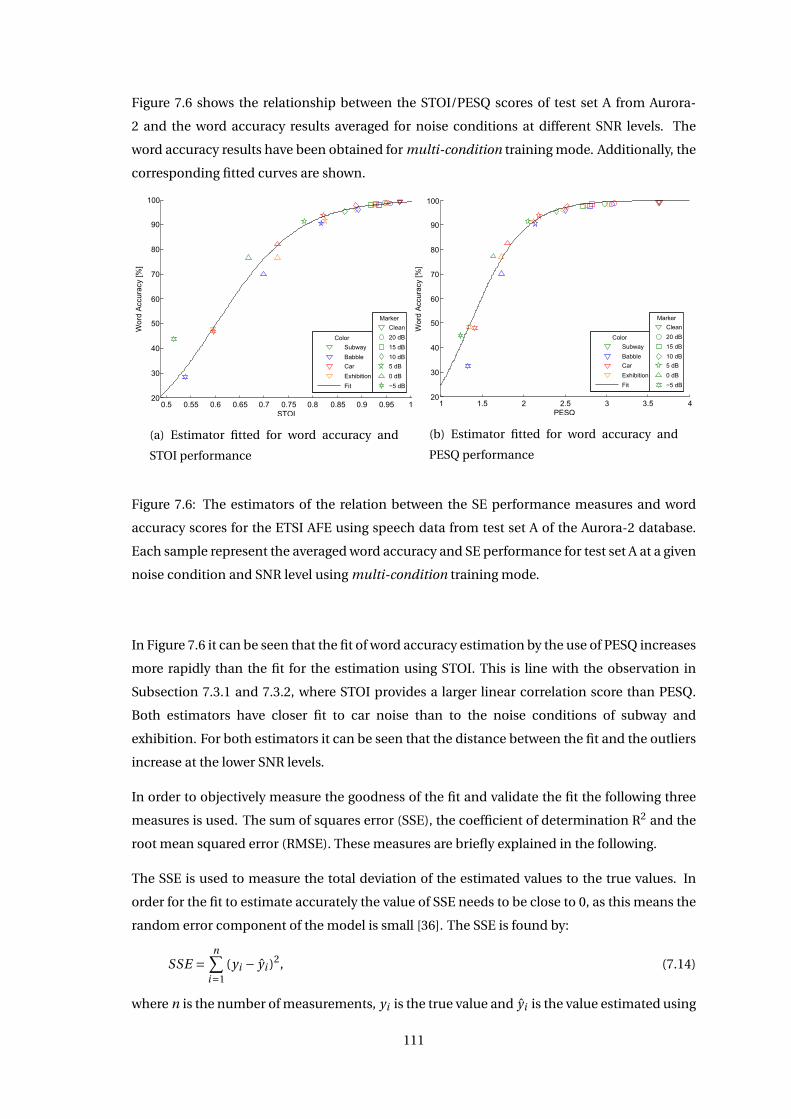
Figure 7.6 shows the relationship between the STOI/PESQ scores of test set A from Aurora-
2 and the word accuracy results averaged for noise conditions at different SNR levels. The
word accuracy results have been obtained for multi-condition training mode. Additionally, the
corresponding fitted curves are shown.
0.5 0.55 0.6 0.65 0.7 0.75 0.8 0.85 0.9 0.95 120
30
40
50
60
70
80
90
100
STOI
Wor
dnA
ccur
acyn
[w]
Clean
20ndB
15ndB
10ndB
5ndB
0ndB
−5ndB
Marker
Subway
Babble
Car
Exhibition
Fit
Color
(a) Estimator fitted for word accuracy and
STOI performance
1 1.5 2 2.5 3 3.5 420
30
40
50
60
70
80
90
100
PESQW
ordn
Acc
urac
yn[w
]
Clean
20ndB
15ndB
10ndB
5ndB
0ndB
−5ndB
Marker
Subway
Babble
Car
Exhibition
Fit
Color
(b) Estimator fitted for word accuracy and
PESQ performance
Figure 7.6: The estimators of the relation between the SE performance measures and word
accuracy scores for the ETSI AFE using speech data from test set A of the Aurora-2 database.
Each sample represent the averaged word accuracy and SE performance for test set A at a given
noise condition and SNR level using multi-condition training mode.
In Figure 7.6 it can be seen that the fit of word accuracy estimation by the use of PESQ increases
more rapidly than the fit for the estimation using STOI. This is line with the observation in
Subsection 7.3.1 and 7.3.2, where STOI provides a larger linear correlation score than PESQ.
Both estimators have closer fit to car noise than to the noise conditions of subway and
exhibition. For both estimators it can be seen that the distance between the fit and the outliers
increase at the lower SNR levels.
In order to objectively measure the goodness of the fit and validate the fit the following three
measures is used. The sum of squares error (SSE), the coefficient of determination R2 and the
root mean squared error (RMSE). These measures are briefly explained in the following.
The SSE is used to measure the total deviation of the estimated values to the true values. In
order for the fit to estimate accurately the value of SSE needs to be close to 0, as this means the
random error component of the model is small [36]. The SSE is found by:
SSE =n∑
i=1(yi − yi )2, (7.14)
where n is the number of measurements, yi is the true value and yi is the value estimated using
111
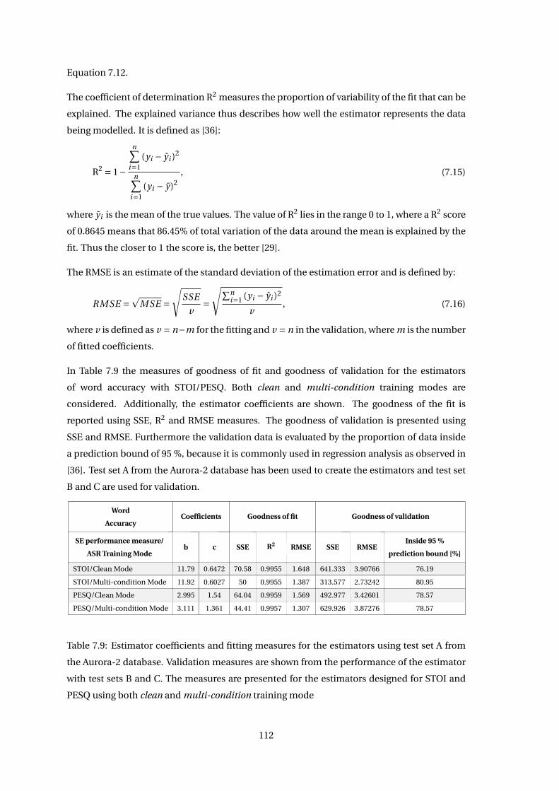
Equation 7.12.
The coefficient of determination R2 measures the proportion of variability of the fit that can be
explained. The explained variance thus describes how well the estimator represents the data
being modelled. It is defined as [36]:
R2 = 1−
n∑i=1
(yi − yi )2
n∑i=1
(yi − y)2, (7.15)
where yi is the mean of the true values. The value of R2 lies in the range 0 to 1, where a R2 score
of 0.8645 means that 86.45% of total variation of the data around the mean is explained by the
fit. Thus the closer to 1 the score is, the better [29].
The RMSE is an estimate of the standard deviation of the estimation error and is defined by:
RMSE =p
MSE =√
SSE
v=
√∑ni=1 (yi − yi )2
v, (7.16)
where v is defined as v = n−m for the fitting and v = n in the validation, where m is the number
of fitted coefficients.
In Table 7.9 the measures of goodness of fit and goodness of validation for the estimators
of word accuracy with STOI/PESQ. Both clean and multi-condition training modes are
considered. Additionally, the estimator coefficients are shown. The goodness of the fit is
reported using SSE, R2 and RMSE measures. The goodness of validation is presented using
SSE and RMSE. Furthermore the validation data is evaluated by the proportion of data inside
a prediction bound of 95 %, because it is commonly used in regression analysis as observed in
[36]. Test set A from the Aurora-2 database has been used to create the estimators and test set
B and C are used for validation.
Word
AccuracyCoefficients Goodness of fit Goodness of validation
SE performance measure/
ASR Training Modeb c SSE R2 RMSE SSE RMSE
Inside 95 %
prediction bound [%]
STOI/Clean Mode 11.79 0.6472 70.58 0.9955 1.648 641.333 3.90766 76.19
STOI/Multi-condition Mode 11.92 0.6027 50 0.9955 1.387 313.577 2.73242 80.95
PESQ/Clean Mode 2.995 1.54 64.04 0.9959 1.569 492.977 3.42601 78.57
PESQ/Multi-condition Mode 3.111 1.361 44.41 0.9957 1.307 629.926 3.87276 78.57
Table 7.9: Estimator coefficients and fitting measures for the estimators using test set A from
the Aurora-2 database. Validation measures are shown from the performance of the estimator
with test sets B and C. The measures are presented for the estimators designed for STOI and
PESQ using both clean and multi-condition training mode
112
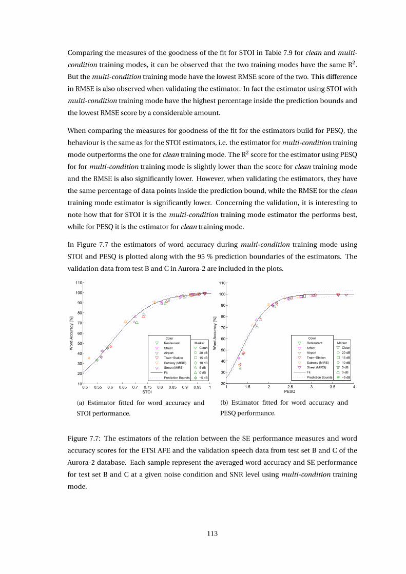
Comparing the measures of the goodness of the fit for STOI in Table 7.9 for clean and multi-
condition training modes, it can be observed that the two training modes have the same R2.
But the multi-condition training mode have the lowest RMSE score of the two. This difference
in RMSE is also observed when validating the estimator. In fact the estimator using STOI with
multi-condition training mode have the highest percentage inside the prediction bounds and
the lowest RMSE score by a considerable amount.
When comparing the measures for goodness of the fit for the estimators build for PESQ, the
behaviour is the same as for the STOI estimators, i.e. the estimator for multi-condition training
mode outperforms the one for clean training mode. The R2 score for the estimator using PESQ
for for multi-condition training mode is slightly lower than the score for clean training mode
and the RMSE is also significantly lower. However, when validating the estimators, they have
the same percentage of data points inside the prediction bound, while the RMSE for the clean
training mode estimator is significantly lower. Concerning the validation, it is interesting to
note how that for STOI it is the multi-condition training mode estimator the performs best,
while for PESQ it is the estimator for clean training mode.
In Figure 7.7 the estimators of word accuracy during multi-condition training mode using
STOI and PESQ is plotted along with the 95 % prediction boundaries of the estimators. The
validation data from test B and C in Aurora-2 are included in the plots.
0P5 0P55 0P6 0P65 0P7 0P75 0P8 0P85 0P9 0P95 110
20
30
40
50
60
70
80
90
100
110
STOI
Wor
dnA
ccur
acyn
[s]
Clean
20ndB
15ndB
10ndB
5ndB
0ndB
−5ndB
MarkerRestaurant
Street
Airport
Train−Station
SubwaynpMIRSb
StreetnpMIRSb
Fit
PredictionnBounds
Color
(a) Estimator fitted for word accuracy and
STOI performance.
1 1)5 2 2)5 3 3)5 420
30
40
50
60
70
80
90
100
110
PESQ
Wor
dnA
ccur
acyn
[s]
Clean
20ndB
15ndB
10ndB
5ndB
0ndB
−5ndB
MarkerRestaurant
Street
Airport
Train−Station
SubwaynpMIRST
StreetnpMIRST
Fit
PredictionnBounds
Color
(b) Estimator fitted for word accuracy and
PESQ performance.
Figure 7.7: The estimators of the relation between the SE performance measures and word
accuracy scores for the ETSI AFE and the validation speech data from test set B and C of the
Aurora-2 database. Each sample represent the averaged word accuracy and SE performance
for test set B and C at a given noise condition and SNR level using multi-condition training
mode.
113
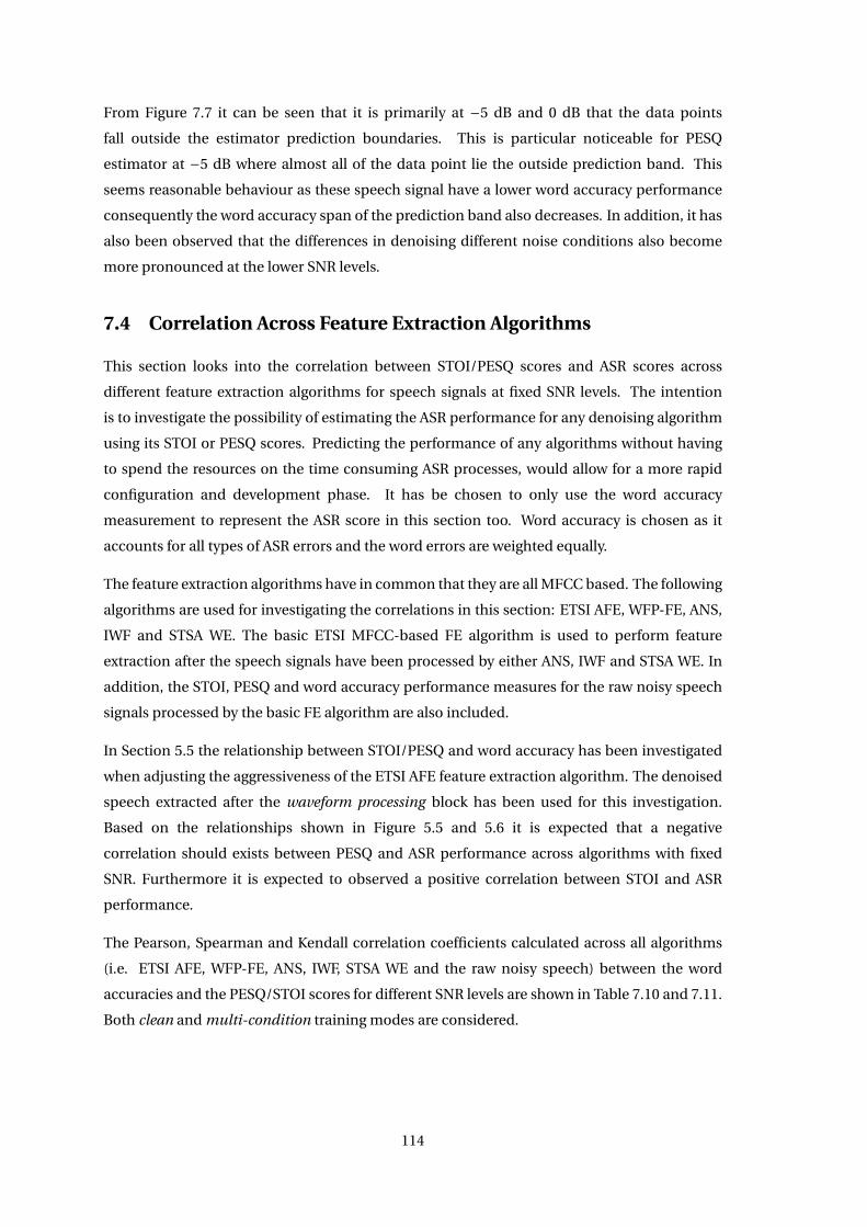
From Figure 7.7 it can be seen that it is primarily at −5 dB and 0 dB that the data points
fall outside the estimator prediction boundaries. This is particular noticeable for PESQ
estimator at −5 dB where almost all of the data point lie the outside prediction band. This
seems reasonable behaviour as these speech signal have a lower word accuracy performance
consequently the word accuracy span of the prediction band also decreases. In addition, it has
also been observed that the differences in denoising different noise conditions also become
more pronounced at the lower SNR levels.
7.4 Correlation Across Feature Extraction Algorithms
This section looks into the correlation between STOI/PESQ scores and ASR scores across
different feature extraction algorithms for speech signals at fixed SNR levels. The intention
is to investigate the possibility of estimating the ASR performance for any denoising algorithm
using its STOI or PESQ scores. Predicting the performance of any algorithms without having
to spend the resources on the time consuming ASR processes, would allow for a more rapid
configuration and development phase. It has be chosen to only use the word accuracy
measurement to represent the ASR score in this section too. Word accuracy is chosen as it
accounts for all types of ASR errors and the word errors are weighted equally.
The feature extraction algorithms have in common that they are all MFCC based. The following
algorithms are used for investigating the correlations in this section: ETSI AFE, WFP-FE, ANS,
IWF and STSA WE. The basic ETSI MFCC-based FE algorithm is used to perform feature
extraction after the speech signals have been processed by either ANS, IWF and STSA WE. In
addition, the STOI, PESQ and word accuracy performance measures for the raw noisy speech
signals processed by the basic FE algorithm are also included.
In Section 5.5 the relationship between STOI/PESQ and word accuracy has been investigated
when adjusting the aggressiveness of the ETSI AFE feature extraction algorithm. The denoised
speech extracted after the waveform processing block has been used for this investigation.
Based on the relationships shown in Figure 5.5 and 5.6 it is expected that a negative
correlation should exists between PESQ and ASR performance across algorithms with fixed
SNR. Furthermore it is expected to observed a positive correlation between STOI and ASR
performance.
The Pearson, Spearman and Kendall correlation coefficients calculated across all algorithms
(i.e. ETSI AFE, WFP-FE, ANS, IWF, STSA WE and the raw noisy speech) between the word
accuracies and the PESQ/STOI scores for different SNR levels are shown in Table 7.10 and 7.11.
Both clean and multi-condition training modes are considered.
114
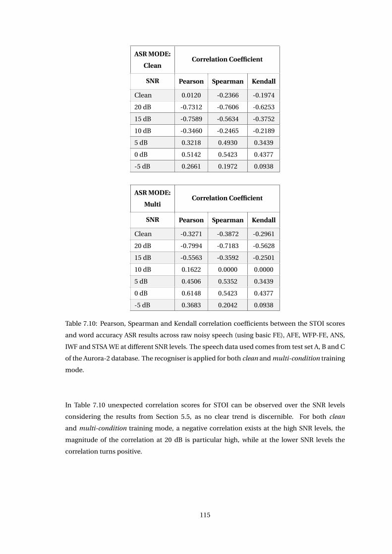
ASR MODE:
CleanCorrelation Coefficient
SNR Pearson Spearman Kendall
Clean 0.0120 -0.2366 -0.1974
20 dB -0.7312 -0.7606 -0.6253
15 dB -0.7589 -0.5634 -0.3752
10 dB -0.3460 -0.2465 -0.2189
5 dB 0.3218 0.4930 0.3439
0 dB 0.5142 0.5423 0.4377
-5 dB 0.2661 0.1972 0.0938
ASR MODE:
MultiCorrelation Coefficient
SNR Pearson Spearman Kendall
Clean -0.3271 -0.3872 -0.2961
20 dB -0.7994 -0.7183 -0.5628
15 dB -0.5563 -0.3592 -0.2501
10 dB 0.1622 0.0000 0.0000
5 dB 0.4506 0.5352 0.3439
0 dB 0.6148 0.5423 0.4377
-5 dB 0.3683 0.2042 0.0938
Table 7.10: Pearson, Spearman and Kendall correlation coefficients between the STOI scores
and word accuracy ASR results across raw noisy speech (using basic FE), AFE, WFP-FE, ANS,
IWF and STSA WE at different SNR levels. The speech data used comes from test set A, B and C
of the Aurora-2 database. The recogniser is applied for both clean and multi-condition training
mode.
In Table 7.10 unexpected correlation scores for STOI can be observed over the SNR levels
considering the results from Section 5.5, as no clear trend is discernible. For both clean
and multi-condition training mode, a negative correlation exists at the high SNR levels, the
magnitude of the correlation at 20 dB is particular high, while at the lower SNR levels the
correlation turns positive.
115
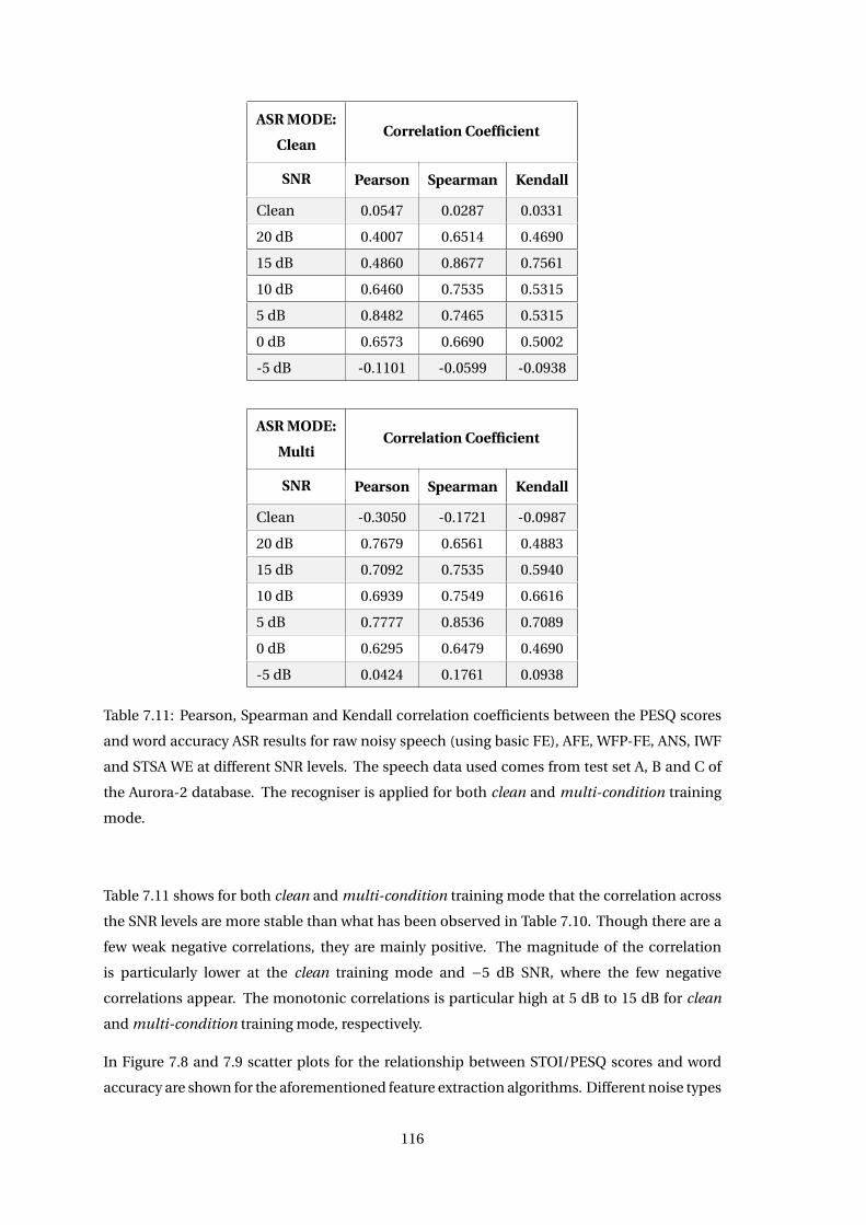
ASR MODE:
CleanCorrelation Coefficient
SNR Pearson Spearman Kendall
Clean 0.0547 0.0287 0.0331
20 dB 0.4007 0.6514 0.4690
15 dB 0.4860 0.8677 0.7561
10 dB 0.6460 0.7535 0.5315
5 dB 0.8482 0.7465 0.5315
0 dB 0.6573 0.6690 0.5002
-5 dB -0.1101 -0.0599 -0.0938
ASR MODE:
MultiCorrelation Coefficient
SNR Pearson Spearman Kendall
Clean -0.3050 -0.1721 -0.0987
20 dB 0.7679 0.6561 0.4883
15 dB 0.7092 0.7535 0.5940
10 dB 0.6939 0.7549 0.6616
5 dB 0.7777 0.8536 0.7089
0 dB 0.6295 0.6479 0.4690
-5 dB 0.0424 0.1761 0.0938
Table 7.11: Pearson, Spearman and Kendall correlation coefficients between the PESQ scores
and word accuracy ASR results for raw noisy speech (using basic FE), AFE, WFP-FE, ANS, IWF
and STSA WE at different SNR levels. The speech data used comes from test set A, B and C of
the Aurora-2 database. The recogniser is applied for both clean and multi-condition training
mode.
Table 7.11 shows for both clean and multi-condition training mode that the correlation across
the SNR levels are more stable than what has been observed in Table 7.10. Though there are a
few weak negative correlations, they are mainly positive. The magnitude of the correlation
is particularly lower at the clean training mode and −5 dB SNR, where the few negative
correlations appear. The monotonic correlations is particular high at 5 dB to 15 dB for clean
and multi-condition training mode, respectively.
In Figure 7.8 and 7.9 scatter plots for the relationship between STOI/PESQ scores and word
accuracy are shown for the aforementioned feature extraction algorithms. Different noise types
116
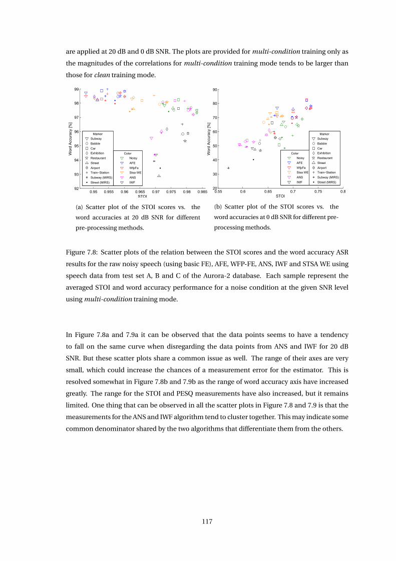
are applied at 20 dB and 0 dB SNR. The plots are provided for multi-condition training only as
the magnitudes of the correlations for multi-condition training mode tends to be larger than
those for clean training mode.
Fk95 Fk955 Fk96 Fk965 Fk97 Fk975 Fk98 Fk98592
93
94
95
96
97
98
99
STOI
Wor
deA
ccur
acye
[i]
e
Subway
Babble
Car
Exhibition
Restaurant
Street
Airport
Train−Station
SubwayeRMIRSs
StreeteRMIRSs
Marker
Noisy
AFE
WfpFe
StsaeWE
ANS
IWF
Color
(a) Scatter plot of the STOI scores vs. the
word accuracies at 20 dB SNR for different
pre-processing methods.
Fk55 Fk6 Fk65 Fk7 Fk75 Fk82F
3F
4F
5F
6F
7F
8F
9F
STOI
Wor
deA
ccur
acye
[i]
e
Subway
Babble
Car
Exhibition
Restaurant
Street
Airport
Train−Station
SubwayeRMIRSs
StreeteRMIRSs
Marker
Noisy
AFE
WfpFe
StsaeWE
ANS
IWF
Color
(b) Scatter plot of the STOI scores vs. the
word accuracies at 0 dB SNR for different pre-
processing methods.
Figure 7.8: Scatter plots of the relation between the STOI scores and the word accuracy ASR
results for the raw noisy speech (using basic FE), AFE, WFP-FE, ANS, IWF and STSA WE using
speech data from test set A, B and C of the Aurora-2 database. Each sample represent the
averaged STOI and word accuracy performance for a noise condition at the given SNR level
using multi-condition training mode.
In Figure 7.8a and 7.9a it can be observed that the data points seems to have a tendency
to fall on the same curve when disregarding the data points from ANS and IWF for 20 dB
SNR. But these scatter plots share a common issue as well. The range of their axes are very
small, which could increase the chances of a measurement error for the estimator. This is
resolved somewhat in Figure 7.8b and 7.9b as the range of word accuracy axis have increased
greatly. The range for the STOI and PESQ measurements have also increased, but it remains
limited. One thing that can be observed in all the scatter plots in Figure 7.8 and 7.9 is that the
measurements for the ANS and IWF algorithm tend to cluster together. This may indicate some
common denominator shared by the two algorithms that differentiate them from the others.
117
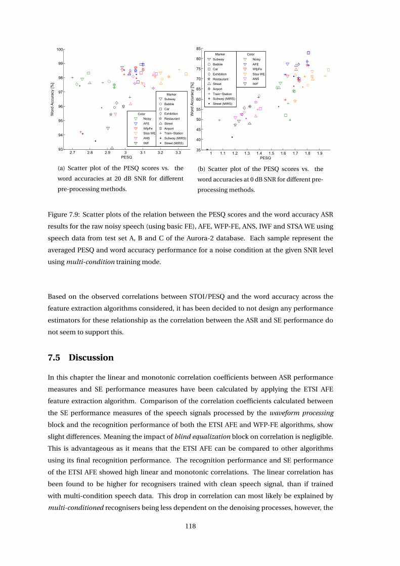
FI7 FI8 FI9 f fIN fIF fIf9f
94
95
96
97
98
99
Nkk
PESQ
Wor
dlA
ccur
acyl
[i]
l
Subway
Babble
Car
Exhibition
Restaurant
Street
Airport
Train−Station
SubwaylRMIRSs
StreetlRMIRSs
Marker
Noisy
AFE
WfpFe
StsalWE
ANS
IWF
Color
(a) Scatter plot of the PESQ scores vs. the
word accuracies at 20 dB SNR for different
pre-processing methods.
N NIN NIF NIf NI4 NI5 NI6 NI7 NI8 NI9f5
4k
45
5k
55
6k
65
7k
75
8k
85
PESQ
Wor
dlA
ccur
acyl
[i]
l
Subway
Babble
Car
Exhibition
Restaurant
Street
Airport
Train−Station
SubwaylRMIRSs
StreetlRMIRSs
Marker
Noisy
AFE
WfpFe
StsalWE
ANS
IWF
Color
(b) Scatter plot of the PESQ scores vs. the
word accuracies at 0 dB SNR for different pre-
processing methods.
Figure 7.9: Scatter plots of the relation between the PESQ scores and the word accuracy ASR
results for the raw noisy speech (using basic FE), AFE, WFP-FE, ANS, IWF and STSA WE using
speech data from test set A, B and C of the Aurora-2 database. Each sample represent the
averaged PESQ and word accuracy performance for a noise condition at the given SNR level
using multi-condition training mode.
Based on the observed correlations between STOI/PESQ and the word accuracy across the
feature extraction algorithms considered, it has been decided to not design any performance
estimators for these relationship as the correlation between the ASR and SE performance do
not seem to support this.
7.5 Discussion
In this chapter the linear and monotonic correlation coefficients between ASR performance
measures and SE performance measures have been calculated by applying the ETSI AFE
feature extraction algorithm. Comparison of the correlation coefficients calculated between
the SE performance measures of the speech signals processed by the waveform processing
block and the recognition performance of both the ETSI AFE and WFP-FE algorithms, show
slight differences. Meaning the impact of blind equalization block on correlation is negligible.
This is advantageous as it means that the ETSI AFE can be compared to other algorithms
using its final recognition performance. The recognition performance and SE performance
of the ETSI AFE showed high linear and monotonic correlations. The linear correlation has
been found to be higher for recognisers trained with clean speech signal, than if trained
with multi-condition speech data. This drop in correlation can most likely be explained by
multi-conditioned recognisers being less dependent on the denoising processes, however, the
118
monotonic correlation remains strong for the multi-condition training mode. Scatterplots
used in conjunction with correlation coefficients revealed that while the STOI measure has
a higher linear correlation than the PESQ measure, both measures follow logistic-like curves.
Estimators have been created inspired by a logistic model presented in [39]. The estimators
have been fitted to a limited data set, where the fitted estimators provide the smallest RMSEs
when considering a multi-condition training mode of ASR. Based on the validation data, the
estimator using STOI to predict the word accuracy of a multi-condition recogniser performs
the best. Although [39] present estimators of ASR performance using PESQ, the authors of
this thesis are not aware of any studies using STOI to predict the ASR performance of feature-
extraction algorithms. Based on the work of this theis, STOI seems to be a viable option
for predicting ASR performance using ETSI AFE. Discouraging results have been obtained
when comparing calculated correlations across different feature-extraction algorithms for
fixed SNRs. Based on the aggressiveness testing in terms of noise reduction from Section 5.5, it
has been anticipated that STOI and PESQ have positive and negative correlations, respectively.
It is possible that they do not behave as expected from the aggressiveness testing, because
the algorithms take fundamentally different approaches to the denoising process. As it can
be observed that some of the algorithms cluster together in the scatterplots, it is possible that
different results might be obtained if using algorithms all based on similar principles.
119

Conclusion 8This thesis investigates the relationship and differences between a noise reduction algorithm
from the field of automatic speech recognition (ASR) and algorithms from the field of speech
enhancement (SE) for human receivers. Estimators of recognition performance are created for
the European telecommunication standards institute (ETSI) advanced frontend (AFE) feature
extraction algorithm using the distortion measures for speech quality and intelligibility. The
perceptual evaluation of speech quality distortion measure estimates speech quality and the
short-time objective intelligibility (STOI) distortion measure estimates speech intelligibility.
Given the performance difference between ETSI AFE and state-of-the-arts SE algorithm in
recognition performance, it is of interest to know if the ETSI AFE perform decently in a speech
enhancement context [14]. Unexpectedly the ETSI AFE preprocessing stages outperform
the state-of-the-art SE methods audible noise suppression (ANS) and the iterative Wiener
filtering (IWF) algorithms designed for human listeners in both PESQ and STOI. However, the
ETSI AFE does not outperform the remaining state-of-the-art method, the short-time spectral
amplitude (STSA) estimator based on the weighted euclidean (WE) distortion measure, in
terms of speech quality as estimated by PESQ. It should be noted that SE performance
measures used are only estimates and listening tests need to be carried out to confirm these
results. In improving the PESQ scores for the SE algorithms designed for human listeners
inadvertently degrade their STOI scores, however, the ETSI AFE preprocessing stages avoids
this degradation. The results concerning recognition performance of ANS, IWF and STSA WE
as feature preprocessing methods agree with the observations made by [14] concerning the
inferior recognition performance of the SE algorithms for human listeners compared to the
ETSI AFE algorithm.
The use of a multi-conditioned recognizer (i.e. acoustic model build using clean and noisy
speech signals) can to some extent compensate for the lack of robustness in ASR performance
using the ANS, IWF and STSA WE algorithms as feature preprocessing methods. The STSA
WE algorithm provides more recognition errors in the noise-only regions of the speech signal
as explored by the use of reference voice activity detection (VAD) labels. The ASR performance
could be enhanced further by improving the behaviour of the STSA WE implementation during
121
noise-only regions. This is demonstrated by frame dropping experiments, where the noise-
only regions of the speech signal is removed using reference VAD labels, where significant
increases in ASR performance has been observed for the STSA WE algorithm when operating
exclusively with speech-only regions. The primary observed difference between the algorithms
from the field of ASR and SE for human listeners is the aggressiveness of the noise reduction
applied. In the spectrogram analysis it has been observed that the ETSI AFE preprocessing
stages preserves more of the noisy speech signals than the STSA WE algorithm. It is suspected
by the authors that this difference in aggressiveness exists as human listeners are superior
to machines in recognising speech and thus require less information to perform recognition
successfully. In addition the SE algorithms for human listeners are expected to operate at lower
signal-to-noise ratios, as human intelligibility is usually not an issue in the expected operating
range of ASR system. Attempts at influencing the aggressiveness of the ETSI AFE and STSA WE
algorithms only produced minor improvements in performance in their rivalling field. This
would make the design of an algorithm to be used in both fields challenging as it would require
a large adjustable range of aggressiveness.
The correlation between the ASR performance across feature extraction algorithms and SE
performance of the corresponding preprocessing stages at fixed SNRs, failed to produce
satisfactory high correlations to justify designing any estimators. However, an estimator has
been designed for the word accuracy performance of the ETSI AFE algorithm. This is based on
the strong correlation between the ASR performance of the ETSI AFE and the SE performance
of the speech signals extracted before feature computation. From the observed relationships
and [40], a logistic model has been chosen for the estimators. The most accurate estimator of
the word accuracy performance of the ETSI AFE, proved to be the one designed for STOI using
a recogniser trained with multi-conditioned speech data. As potential future work we propose
investigating the performance of a STOI based estimator of word accuracy for other feature
extraction methods. In addition the performance of ANS and IWF when frame dropping with
reference VAD is applied should be investigated.
122
References
[1] C. Bishop. Pattern Recognition and Machine Learning. Springer, 2006.
[2] P. Y. Chen and P. M. Popovich. Correlation. SAGE Publications, Inc., 2002.
[3] Deller, Jr., J. R. and Hansen, J. H. L. and Proakis, J. G. Discrete-Time Processing of Speech
Signals. Wiley-IEEE Press, 1999.
[4] Encyclopaedia Britannica. Tympanic Membrane. http://global.britannica.com/
EBchecked/topic/611539/tympanic-membrane, 1997.
[5] Y. Ephraim and D. Malah. Speech Enhancement Using a Minimum-mean Square Error
Short-time Spectral Amplitude Estimator. Acoustics, Speech and Signal Processing, IEEE
Transactions on, 32(6):1109–1121, Dec 1984.
[6] ETSI Standard ES 201 108. Speech Processing, Transmission and Quality Aspects (STQ);
Distributed Speech Recognition; Front-end Feature Extraction Algorithm; Compression
Algorithms. ETSI Standard, ETSI, Apr 2000.
[7] ETSI Standard ES 202 050. Speech Processing, Transmission and Quality Aspects (STQ);
Distributed Speech Recognition; Extended Front-end Feature Extraction Algorithm;
Compression Algorithms. ETSI Standard, ETSI, Jan 2007.
[8] S. A. Gelfand. Hearing - An Introduction to Psychological and Physiological Acoustics.
Marcel Dekker, 4 edition, 2004.
[9] M. Greenacre. Correspondence Analysis in Practice. Chapman and Hall/CRC , 2 edition,
2007.
[10] J. Hansen. Analysis and Compensation of Stressed and Noisy Speech with Application to
Robust Automatic Recognition. PhD thesis, Georgia Institute of Technology, 1988.
[11] Hendriks, R. C. and Gerkmann, T and Jensen, J. DFT-Domain Based Single-Microphone
Noise Reduction for Speech Enhancement: A Survey of the State-of-the-Art. Morgan &
Claypool, 2013.
[12] G. Hirsch and D. Pearce. Applying the Advanced ETSI Frontend to the Aurora-2 Task.
Technical report, 2006.
123
[13] D. M. Howard and J. Angus. Acoustics and Phychoacoustics. Elsevier, 3 edition, 2006.
[14] J. Jensen and Z.-H. Tan. Minimum Mean-Square Error Estimation of Mel-Frequency
Cepstral Features - A Theoretically Consistent Approach. Audio, Speech, and Language
Processing, IEEE/ACM Transactions on, 23(1):186–197, Jan 2015.
[15] J.S. Lim and A.V. Oppenheim. All-Pole Modeling of Degraded Speech. Acoustics, Speech
and Signal Processing, IEEE Transactions on, 26(3):197–210, Jun 1978.
[16] P. C. Loizou. Speech Enhancement: Theory and Practice. CRC Press, 2007.
[17] P. C. Loizou. Speech Enhancement: Theory and Practice. CRC Press, 2 edition, 2013.
[18] P.C. Loizou. Speech Enhancement Based on Perceptually Motivated Bayesian Estimators
of the Magnitude Spectrum. Speech and Audio Processing, IEEE Transactions on, 13(5):
857–869, Sep 2005.
[19] V. K. Madisetti. The Digital Signal Processing Handbook - Digital Signal Processing
Fundamentals. CRC Press, 2 edition, 2010.
[20] Curve Fitting ToolboxTM User’s Guide. The MathWorks, Inc, 2015.
[21] A. R. Møller. Hearing - Its Physiology and Pathphysiology. Academic Press, 2000.
[22] B. C. J. Moore. Cochlear Hearing Loss: Physiological, Psychological and Technical Issues.
John Wiley & Sons, 2007.
[23] B. C. J. Moore. An Introduction to the Psychology of Hearing. Emerald, 5 edition, 2008.
[24] J. L. Myers and A. D. Well. Research Design and Statistical Analysis. L. Erlbaum, 2 edition,
2003.
[25] D. O’Shaughnessy. Speech Communication: Human and Machine. Addison Wesley, 1987.
[26] D. Pearce, H. Hirsch, and Ericsson Eurolab Deutschland Gmbh. The Aurora Experimental
Framework for the Performance Evaluation of Speech Recognition Systems under Noisy
Conditions. In ISCA ITRW ASR2000, pages 29–32, 2000.
[27] A. Peinado and J. Segura. Speech Recognition Over Digital Channels: Robustness and
Standards. Wiley, 2006.
[28] Quatieri, T. F. Discrete-Time Speech Signal Processing: Principles and Practice. Prentice
Hall PTR, 2002.
[29] A. Sen and M. Srivastava. Regression Analysis - Theory, Methods, and Applications.
Springer-Verlag, 1990.
124
[30] S. Sigurdsson, K. B. Petersen, and T. Lehn-Schiøler. Mel Frequency Cepstral Coefficients:
An Evaluation of Robustness of mp3 Encoded Music. Seventh International Conference on
Music Information Retrieval (ISMIR), 2006.
[31] S. S. Stevens, J. Volkmann, and E. B. Newman. A Scale for the Measurement of the
Psychological Magnitude Pitch. The Journal of the Acoustical Society of America, 8(3):185–
190, 1937.
[32] C. H. Taal, R. C. Hendriks, R. Heusdens, and J. Jensen. A Short-Time Objective Intelligibility
Measure for Time-Frequency Weighted Noisy Speech. In Acoustics Speech and Signal
Processing (ICASSP), 2010 IEEE International Conference on, pages 4214–4217. IEEE, 2010.
[33] Z.-H. Tan and B. Lindberg. Automatic Speech Recognition on Mobile Devices and over
Communication Networks. Springer, 2008.
[34] Z.-H. Tan and B. Lindberg. Low-complexity Variable Frame Rate Analysis for Speech
Recognition and Voice Activity Detection. IEEE Journal of Selected Topics in Signal
Processing, 4(5):798–807, Sep 2010.
[35] Tan, Z.-H. Noise-robust Voice Activity Detection (rVAD) - Source Code, Reference VAD for
Aurora 2. http://kom.aau.dk/~zt/online/rVAD/, Dec 2014.
[36] M. D. Ugarte, A. F. Militino, and A. T. Arnholt. Probability and Statistics with R. Chapman
and Hall/CRC, 2008.
[37] T. Virtanen, R. Singh, and B. Raj. Techniques for Noise Robustness in Automatic Speech
Recognition. John Wiley & Sons, 2012.
[38] M. Woelfel and J. McDonough. Distant Speech Recognition. John Wiley & Sons, 2009.
[39] T. Yamada and N. Kitawaki. A PESQ-based Performance Prediction Method for Noisy
Speech Recognition. Proc. International Congress on Acoustics, 2:1695–1698, Apr 2004.
[40] T. Yamada, M. Kumakura, and N. Kitawaki. Performance Estimation of Speech
Recognition System Under Noise Conditions Using Objective Quality Measures and
Artificial Voice. Audio, Speech, and Language Processing, IEEE Transactions on, 14(6):
2006–2013, Nov 2006.
[41] S. Young, G. Evermann, M. Gales, T. Hain, D. Kershaw, X. Liu, G. Moore, J. Odell, D. Ollason,
D. Povey, V. Valtchev, and P. Woodland. The HTK Book (for HTK Version 3.4). Cambridge
University Engineering Department, 2009.
125

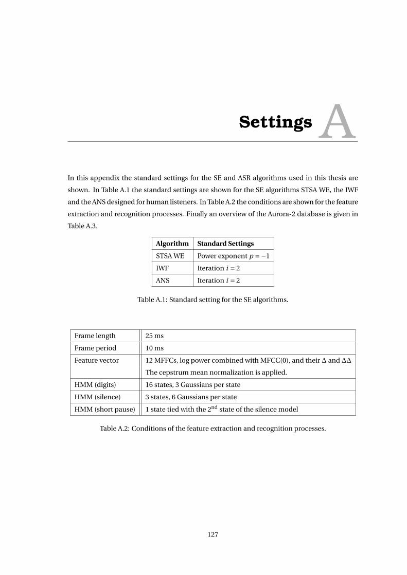
Settings AIn this appendix the standard settings for the SE and ASR algorithms used in this thesis are
shown. In Table A.1 the standard settings are shown for the SE algorithms STSA WE, the IWF
and the ANS designed for human listeners. In Table A.2 the conditions are shown for the feature
extraction and recognition processes. Finally an overview of the Aurora-2 database is given in
Table A.3.
Algorithm Standard Settings
STSA WE Power exponent p =−1
IWF Iteration i = 2
ANS Iteration i = 2
Table A.1: Standard setting for the SE algorithms.
Frame length 25 ms
Frame period 10 ms
Feature vector 12 MFFCs, log power combined with MFCC(0), and their ∆ and ∆∆
The cepstrum mean normalization is applied.
HMM (digits) 16 states, 3 Gaussians per state
HMM (silence) 3 states, 6 Gaussians per state
HMM (short pause) 1 state tied with the 2nd state of the silence model
Table A.2: Conditions of the feature extraction and recognition processes.
127
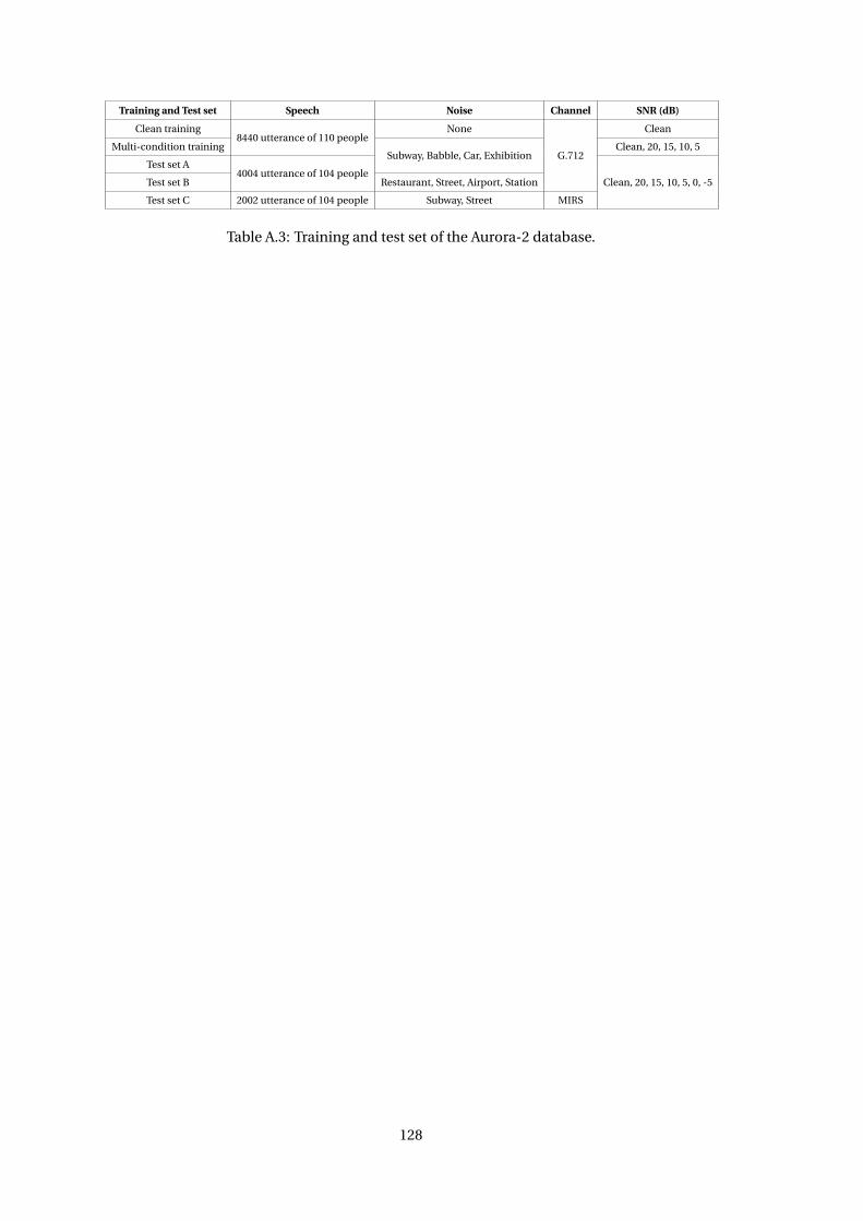
Training and Test set Speech Noise Channel SNR (dB)
Clean training8440 utterance of 110 people
None
G.712
Clean
Multi-condition trainingSubway, Babble, Car, Exhibition
Clean, 20, 15, 10, 5
Test set A4004 utterance of 104 people
Clean, 20, 15, 10, 5, 0, -5Test set B Restaurant, Street, Airport, Station
Test set C 2002 utterance of 104 people Subway, Street MIRS
Table A.3: Training and test set of the Aurora-2 database.
128
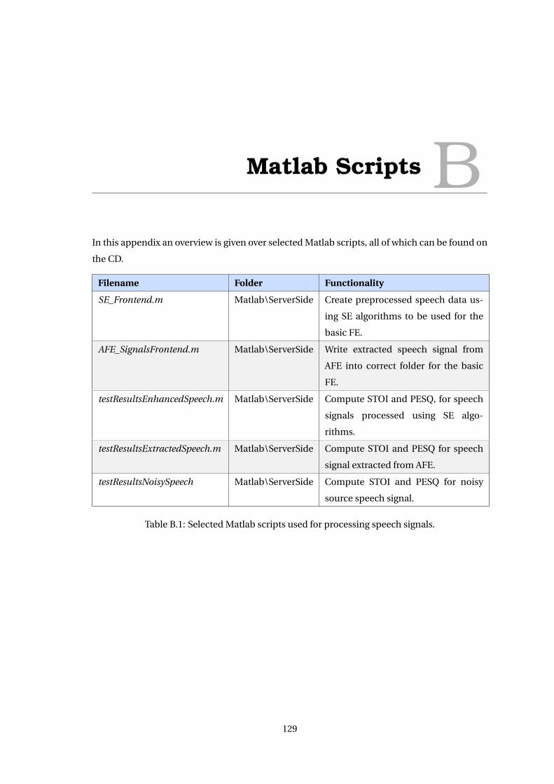
Matlab Scripts BIn this appendix an overview is given over selected Matlab scripts, all of which can be found on
the CD.
Filename Folder Functionality
SE_Frontend.m Matlab\ServerSide Create preprocessed speech data us-
ing SE algorithms to be used for the
basic FE.
AFE_SignalsFrontend.m Matlab\ServerSide Write extracted speech signal from
AFE into correct folder for the basic
FE.
testResultsEnhancedSpeech.m Matlab\ServerSide Compute STOI and PESQ, for speech
signals processed using SE algo-
rithms.
testResultsExtractedSpeech.m Matlab\ServerSide Compute STOI and PESQ for speech
signal extracted from AFE.
testResultsNoisySpeech Matlab\ServerSide Compute STOI and PESQ for noisy
source speech signal.
Table B.1: Selected Matlab scripts used for processing speech signals.
129
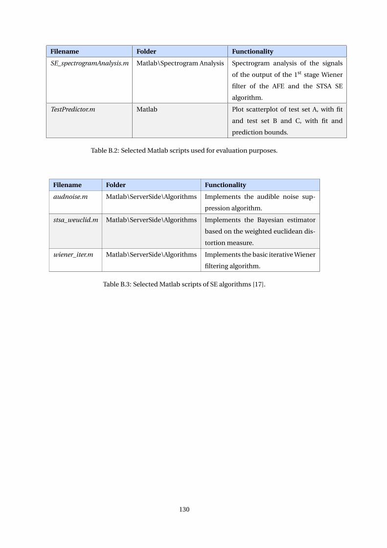
Filename Folder Functionality
SE_spectrogramAnalysis.m Matlab\Spectrogram Analysis Spectrogram analysis of the signals
of the output of the 1st stage Wiener
filter of the AFE and the STSA SE
algorithm.
TestPredictor.m Matlab Plot scatterplot of test set A, with fit
and test set B and C, with fit and
prediction bounds.
Table B.2: Selected Matlab scripts used for evaluation purposes.
Filename Folder Functionality
audnoise.m Matlab\ServerSide\Algorithms Implements the audible noise sup-
pression algorithm.
stsa_weuclid.m Matlab\ServerSide\Algorithms Implements the Bayesian estimator
based on the weighted euclidean dis-
tortion measure.
wiener_iter.m Matlab\ServerSide\Algorithms Implements the basic iterative Wiener
filtering algorithm.
Table B.3: Selected Matlab scripts of SE algorithms [17].
130