speech feature toolbox (speft) design and emotional …speech feature extraction plays an important...
TRANSCRIPT

SPEech Feature Toolbox (SPEFT) Design and Emotional Speech Feature Extraction
by
Xi Li
A thesis submitted to the Faculty of Graduate School, Marquette University,
in Partial Fulfillment of the Requirements for the Degree of Master of Science
Milwaukee, Wisconsin
August, 2007

Preface
This research focuses on designing the SPEech Feature Toolbox (SPEFT), a toolbox
which integrates a large number of speech features into one graphic interface in the MATLAB environment. The toolbox is designed with a Graphical User Interface (GUI) interface which makes it easy to operate; it also provides batch process capability. Available features are categorized into sub-groups including spectral features, pitch frequency detection, formant detection, pitch related features and other time domain features.
A speaking style classification experiment is carried out to demonstrate the use of
the SPEFT toolbox, and validate the usefulness of non-traditional features in classifying different speaking styles. The pitch-related features jitter and shimmer are combined with the traditional spectral and energy features MFCC and log energy. A Hidden Markov Models (HMMs) classifier is applied to these combined feature vectors, and the classification results between different feature combinations are compared. A thorough test of the SPEFT toolbox is also presented by comparing the extracted feature results between SPEFT and previous toolboxes across a validation test set.

Acknowledgements
I thank my advisor, Dr. Michael Johnson for giving me this precious opportunity to work in his speech group under NSF’s Dr. Do-little project, and for the generous help and insightful guidance he has offered me in the past two years.
I thank my master’s thesis committee for their support and helpful reviews, Dr.
Richard Povinelli and Dr. Craig Struble. I thank my colleagues, Marek, Yao, Jidong and Patrick, who constantly and
generously shared their knowledge in their research fields. Most importantly, I would like to express gratitude to my parents and family
members, who have been the inspiration throughout this journey. Finally, I thank all the collaborators under Dr. Do-little project, the well labeled data
and their time-cosuming work significantly facilitated the process this research.

Table of Contents i
TABLE OF CONTENTS
TABLE OF CONTENTS .................................................................................................. I
LIST OF FIGURES ........................................................................................................ IV
LIST OF TABLES ........................................................................................................... V
CHAPTER 1 INTRODUCTION AND RESEARCH OBJECTIVES .......................... 1
1.1 GENERAL BACKGROUND ...................................................................................... 1 1.2 OBJECTIVE OF THE RESEARCH ............................................................................ 3 1.3 ORGANIZATION OF THE THESIS ........................................................................... 5
CHAPTER 2 BACKGROUND ON SPEECH FEATURE EXTRACTION ............... 6
2.1 OVERVIEW ............................................................................................................ 6 2.2 PREPROCESSING ................................................................................................... 7
2.2.1 DC Component Removal ............................................................................. 7 2.2.2 Preemphasis Filtering .................................................................................. 7 2.2.3 Amplitude Normalization ............................................................................ 8
2.3 WINDOWING ......................................................................................................... 8 2.3.1 Windowing Functions .................................................................................. 9 2.3.2 Traditional Framing Method ...................................................................... 9 2.3.3 Fixed Step Size Framing Method ............................................................. 10
2.4 SPECTRAL FEATURES ......................................................................................... 11 2.4.1 Mel-Frequency Cepstral Coefficient (MFCC) ........................................ 11 2.4.2 Greenwood Function Cepstral Coefficient (GFCC) ............................... 14 2.4.3 Perceptual Linear Prediction (PLP), gPLP and RASTA-PLP .............. 16 2.4.4 Linear Prediction Filter Coefficient (LPC) and LPC-related Features 21
2.5 PITCH DETECTION ALGORITHMS ...................................................................... 23 2.5.1 Autocorrelation Pitch Detection ............................................................... 23 2.5.2 Cepstral Pitch Detection ............................................................................ 25 2.5.3 Average Magnitude Different Function (AMDF) ................................... 26 2.5.4 Robust Algorithm for Pitch Tracking (RAPT) ....................................... 27 2.5.5 Post-processing ........................................................................................... 29
2.6 FORMANT EXTRACTION TECHNIQUES .............................................................. 29 2.6.1 Formant Estimation by LPC Root-Solving Procedure........................... 30 2.6.2 Adaptive Bandpass Filterbank Formant Tracker .................................. 32
2.7 PITCH-RELATED FEATURES ............................................................................... 35 2.7.1 Jitter ............................................................................................................ 36

Table of Contents ii
2.7.2 Shimmer ...................................................................................................... 37 2.8 LOG ENERGY AND DELTA FEATURES ................................................................ 37
2.8.1 Log Energy ................................................................................................. 37 2.8.2 Delta Features ............................................................................................. 38
CHAPTER 3 SPEECH FEATURE TOOLBOX (SPEFT) DESIGN ........................... 39
3.1 REVIEW OF PREVIOUS SPEECH TOOLBOXES ..................................................... 40 3.1.1 Hidden Markov Toolkit (HTK) ................................................................ 40 3.1.2 COLEA Toolbox ........................................................................................ 42 3.1.3 Voice Box .................................................................................................... 44
3.2 MATLAB GRAPHICAL USER INTERFACE (GUI) INTRODUCTION ................... 45 3.3 SPEECH FEATURE TOOLBOX (SPEFT) DESIGN .................................................. 46
3.3.1 GUI Layout ................................................................................................. 46 3.3.2 Batch Processing Mode.............................................................................. 49 3.3.3 Hierarchical Feature with Different Window Size ................................. 50 3.3.4 Extensibility ................................................................................................ 52 3.3.5 Integrated Speech Features ....................................................................... 52
CHAPTER 4 SPEAKING STYLE CLASSIFICATION USING SPEFT ................. 55
4.1 INTRODUCTION ................................................................................................... 56 4.2 EXPERIMENT OUTLINE ...................................................................................... 57
4.2.1 SUSAS Database ........................................................................................ 57 4.2.2 Acoustic Models ......................................................................................... 58
4.3 SPEECH FEATURE EXTRACTION PROCESS ........................................................ 60 4.4 SPEAKING STYLE CLASSIFICATION BASED ON SUSAS..................................... 64 4.5 EXPERIMENT RESULTS AND DISCUSSION .......................................................... 65 4.6 CONCLUSIONS ..................................................................................................... 66
CHAPTER 5 SPEFT TESTING .................................................................................... 69
5.1 SOFTWARE TESTING BASICS .............................................................................. 69 5.2 STANDARD TESTING DATA ................................................................................. 72 5.3 TESTING METHOD .............................................................................................. 74 5.4 TESTING EXPERIMENTS ..................................................................................... 75
5.4.1 System Testing ............................................................................................ 75 5.4.2 Component Testing .................................................................................... 76 5.4.3 Acceptance Testing .................................................................................... 76
5.5 TESTING RESULTS .............................................................................................. 76 5.5.1 MFCCs ........................................................................................................ 76 5.5.2 PLP .............................................................................................................. 79 5.5.3 LPC, LPC Reflection Coefficients and LPC Cepstral Coefficients ....... 83 5.5.4 Pitch and formant ...................................................................................... 83

Table of Contents iii
5.5.5 Energy ......................................................................................................... 84 5.6 CONCLUSION ...................................................................................................... 87
CHAPTER 6 CONCLUSIONS ...................................................................................... 89
APPENDIX ...................................................................................................................... 97
INSTALLATION INSTRUCTIONS ..................................................................................... 98 GETTING STARTED ........................................................................................................ 99 GUIDED EXAMPLE ....................................................................................................... 100 BUTTONS ON THE MAIN INTERFACE OF SPEFT ........................................................ 104 VARIABLES IN WORK SPACE ...................................................................................... 107 BATCH PROCESSING MODE ........................................................................................ 109 EXTENSIBILITY ............................................................................................................ 111 INTEGRATED ALGORITHMS AND ADJUSTABLE PARAMETERS ................................... 113
1) Spectral Features: .............................................................................................. 113 2) Pitch Tracking Algorithms:............................................................................... 116 3) Formant Tracking Algorithms: ......................................................................... 117 4) Features used in speaking style classification: .................................................. 117 5) Other features: ................................................................................................... 118

List of Figures iv
LIST OF FIGURES
Figure 2.1: MFCC Extraction Block Diagram .................................................................. 13 Figure 2.2: GFCC Extraction Block Diagram .................................................................. 15 Figure 2.3: Extraction Flow Graph of PLP, gPLP and RASTA-PLP Features ................. 20 Figure 2.4: Flow Graph of the Autocorrelation Pitch Detector ........................................ 25 Figure 2.5: Flow Graph of Cepstral Pitch Detector .......................................................... 26 Figure 2.6: Flow Graph of the AMDF Pitch Detector ...................................................... 27 Figure 2.7: Block Diagram of the Robust Formant Tracker ............................................. 33 Figure 3.1: COLEA toolbox main interface ...................................................................... 43 Figure 3.2: GUI Layout of the Main Interface .................................................................. 47 Figure 3.3: MFCC Parameter Configuration Interface GUI Layout ................................. 48 Figure 3.4: LPC Parameter Configuration Interface GUI Layout .................................... 49 Figure 3.5: Batch File Processing Interface Layout.......................................................... 50 Figure 3.6: Comparison between traditional and fixed step size framing method ........... 52 Figure 4.1: HMM for Speech Recognition ....................................................................... 59 Figure 4.2: Jitter Parameter Configurations in SPEFT ..................................................... 62 Figure 4.3: Shimmer Parameter Configurations in SPEFT .............................................. 62 Figure 4.4: MFCCs Parameter Configurations in SPEFT ................................................ 63 Figure 4.5: Energy Parameter Configurations in SPEFT .................................................. 63 Figure 4.6: Classification Results use MFCCs and Energy features ................................ 67 Figure 4.7: Classification Results by Combining Baseline Features and Pitch-related Features ............................................................................................................................. 68 Figure 5.1: Testing Process ............................................................................................... 70 Figure 5.2: Testing Phases in Software Process ................................................................ 70 Figure 5.3: MFCC Parameter Configuration Interface in SPEFT .................................... 78 Figure 5.4: PLP Parameter Configuration Interface in SPEFT ......................................... 81 Figure 5.5: Energy Parameter Configuration Interface in SPEFT .................................... 85

List of Tables v
LIST OF TABLES
Table 4.1: Summary of the SUSAS Vocabulary ............................................................... 58 Table 4.2: Speech Features Extracted from Each Frame .................................................. 61 Table 4.3: Comparison Between SPEFT & HTK Classification Results Using MFCCs and Energy features ........................................................................................................... 67 Table 4.4: HTK Classification Results Using Different Feature Combinations ............... 68 Table 5.1: MFCC Test Results .......................................................................................... 79 Table 5.2 PLP Test Results ................................................................................................ 82 Table 5.3: LPC Related Features Test Results .................................................................. 83 Table 5.4: Normalized Energy Features Test Results ....................................................... 86 Table 5.5 Un-normalized Energy Features Test Results ................................................... 87

Chapter 1 Introduction and Research Objectives 1
Chapter 1
Introduction and Research Objectives
1.1 General Background
Speech feature extraction plays an important role in speech signal processing
research. From automatic speech recognition to spoken language synthesis, from basic
applications such as speech coding to the most advanced technology such as automatic
translation, speech signal processing applications are closely related to the extraction of
speech features.
To facilitate the speech feature extraction process, researchers have implemented
many of the algorithms and integrated them together as toolboxes. These toolboxes
significantly reduce the labor cost and increase the reliability in extracting speech
features. However, there are several problems that exist in current tools. First, the speech
features implemented are relatively limited, so that typically only the energy features and
basic spectral domain features are provided. Also, the operation of existing toolboxes is
complex and inconvenient to use due to the use of command line interfaces. Finally,
many don’t have batch capability to manage large file sets. All the above problems hinder

Chapter 1 Introduction and Research Objectives 2
the usage in research, especially when dealing with a large volume of source files.
As speech signal processing research continues, there are many newly proposed
features being developed [1, 2]. Because previous toolboxes for speech feature extraction
do not adequately cover these newer used features, these toolboxes have become outdated.
For example, there has been a lot of interest in researching speech speaking style
classification and emotion recognition in recent years. Previous research has shown a
high correlation between features based on fundamental frequency and the emotional
states of the speakers [3]. Speech features that characterize fundamental frequency
patterns reflect the difference between speaking styles and emotions are helpful for
improving classification results. Examples of such features are jitter and shimmer, which
are defined as the short-term change in the fundamental frequency and amplitude,
respectively. Features like jitter and shimmer are commonly employed in speech research
since they are representative of speaker, language, and speech content. Classification
accuracy can be increased by combining these features with conventional spectral and
energy features in emotion recognition tasks [2]. However, none of the current speech
toolboxes can extract these features.
Additionally, most of the current toolboxes are difficult to operate. They often rely
on complex command line interfaces, as opposed to having a Graphical User Interface
(GUI), which is much easier for users to interact with. For instance, the Hidden Markov
Toolkit (HTK), a toolbox developed at the Machine Intelligence Laboratory of the

Chapter 1 Introduction and Research Objectives 3
Cambridge University Engineering Department, is primarily designed for building and
manipulating hidden Markov models in speech recognition research. The toolbox
includes algorithms to extract multiple speech features. However, due to its command
line operation interface, it may take many hours of study before one can actually use the
toolbox to accomplish any classification task. The feature extraction procedure would be
much easier if a large number of algorithms were integrated into a toolbox with a GUI
interface.
In addition, speech recognition research usually requires extracting speech features
from hundreds or even thousands of different source files. Many current toolboxes often
do not have batch capability to handle tasks that include a large number of source files.
An example of this is the COLEA toolbox used for speech analysis in MATLAB [4].
Although it has a GUI interface which greatly facilitates operation, the toolbox can only
extract features from at most two speech files each time due to the lack of batch file
processing capability. The limitation to analysis and display of only one or two source
files means the applicability of the toolbox is significantly restricted.
1.2 Objective of the Research
This research focuses on designing the SPEech Feature Toolbox (SPEFT), a toolbox
which integrates a large number of speech features into one graphic interface in the
MATLAB environment. The goal is to help users conveniently extract a wide range of

Chapter 1 Introduction and Research Objectives 4
speech features and generate files for further processing. The toolbox is designed with a
GUI interface which makes it easy to operate; it also provides batch process capability.
Available features are categorized into sub-groups including spectral features, pitch
frequency detection, formant detection, pitch related features and other time domain
features.
Extracted feature vectors are written into HTK file format which have the
compatibility with HTK for further classifications. To synchronize the time scale between
different features, the SPEFT toolbox employs a fixed step size windowing method. This
is to extract different features with the same step size while keep each feature’s own
window length. The ability to incorporate multiple window sizes is unique to SPEFT.
To demonstrate the use of the SPEFT toolbox, and validate the usefulness of
non-traditional features in classifying different speaking styles, a speaking style
classification experiment is carried out. The pitch-related features jitter and shimmer are
combined with the traditional spectral and energy features MFCC and log energy. A
Hidden Markov Model (HMM) classifier is applied to these combined feature vectors,
and the classification results between different feature combinations are compared. Both
jitter and shimmer features are extracted by SPEFT. A thorough test of the SPEFT
toolbox is presented by comparing the extracted feature results between SPEFT and
previous toolboxes across a validation test set.
The user manual and source code of the toolbox are available form the MATLAB

Chapter 1 Introduction and Research Objectives 5
Central File Exchange and the Marquette University Speech Lab websites.
1.3 Organization of the Thesis
The thesis consists of six chapters. Chapter 1 provides a general overview of the
current speech feature extraction toolbox designs, and the objectives of the thesis.
Chapter 2 gives background knowledge on features integrated into SPEFT. In Chapter 3,
an in depth analysis of previous toolboxes is provided, followed by details of the SPEFT
Graphic User Interface design. Chapter 4 introduces a speaking style classification
experiment which verifies the usefulness of the toolbox design. Results and conclusions
of the experiments are provided at the end of this Chapter. Chapter 5 discusses the testing
methods, and also gives verification results by comparing the features extracted by
SPEFT and existing toolboxes. The final chapter provides of this thesis provides a
conclusion of the thesis. The appendices contain examples of code from the speech
feature toolbox and a copy of the user manual.

Chapter 2 Background on Speech Feature Extraction 6
Chapter 2
2 Background on Speech Feature Extraction
2.1 Overview
Speech feature extraction is a fundamental requirement of any speech recognition
system; it is the mathematic representation of the speech file. In a human speech
recognition system, the goal is to classify the source files using a reliable representation
that reflects the difference between utterances.
In the SPEFT toolbox design, a large number of speech features are included for
user configuration and selection. Integrated features are grouped into the following five
categories: spectral features, pitch frequency detection, formant detection, pitch-related
features and other time domain features. Some of the features included are not commonly
seen in regular speech recognition systems.
This chapter outlines the extraction process of the features that are employed in
SPEFT design.

Chapter 2 Background on Speech Feature Extraction 7
2.2 Preprocessing
Preprocessing is the fundamental signal processing applied before extracting
features from speech signal, for the purpose of enhancing the performance of feature
extraction algorithms. Commonly used preprocessing techniques include DC component
removal, preemphasis filtering, and amplitude normalization. The SPEFT toolbox allows
a user to combine these preprocessing blocks and define their parameters.
2.2.1 DC Component Removal
The initial speech signal often has a constant component, i.e. a non-zero mean. This
is typically due to DC bias within the recording instruments. The DC component can be
easily removed by subtracting the mean value from all samples within an utterance.
2.2.2 Preemphasis Filtering
A pre-emphasis filter compresses the dynamic range of the speech signal’s power
spectrum by flattening the spectral tilt. Typically, the filter is in form of
( ) 11 −−= azzP , (2.1)
where a ranges between 0.9 and 1.0. In SPEFT design, the default value is set to 0.97.
In speech processing, the glottal signal can be modeled by a two-pole filter with
both poles close to the unit circle [5]. However, the lip radiation characteristic models its
single zero near z=1, which tends to cancel the effect of one glottal pole. By incorporating

Chapter 2 Background on Speech Feature Extraction 8
a preemphasis filter, another zero is introduced near the unit circle which effectively
eliminating the lip radiation effect [6].
In addition, the spectral slope of a human speech spectrum is usually negative since
the energy is concentrated in low frequency. Thus, a preemphasis filter is introduced
before applying feature algorithms to increase the relative energy of the high-frequency
spectrum.
2.2.3 Amplitude Normalization
Recorded signals often have varying energy levels due to speaker volume and
microphone distance. Amplitude Normalization can cancel the inconsistent energy level
between signals, thus can enhance the performance in energy-related features.
There are several methods to normalize a signal’s amplitude. One of them is
achieved by a point-by-point division of the signal by its maximum absolute value, so
that the dynamic range of the signal is constrained between -1.0 and +1.0. Another
commonly used normalization method is to divide each sample point by the variance of
an utterance.
In SPEFT design, signals can be optionally normalized by division of its maximum
value.
2.3 Windowing

Chapter 2 Background on Speech Feature Extraction 9
2.3.1 Windowing Functions
Speech is a non-stationary signal. To approximate a stationary signal, a window
function is applied in the preprocessing stage to divide the speech signal into small
segments. A simple rectangular window function zeros all samples outside the given
frame and maintains the amplitude of those samples within its frame.
When applying a spectral analysis such as a Fast Fourier Transform (FFT) to a
frame of rectangular windowed signal, the abrupt change at the starting and ending point
significantly distorts the original signal in the frequency domain. To alleviate this
problem, the rectangular window function is modified, so that the points close to the
beginning and the end of each window slowly attenuate to zero. There are many possible
window functions. One common type is the generalized Hamming window, defined as
( ) ( )[ ]⎩⎨⎧
=−≤≤−−−
=elsen
NnNnnw
0101/2cos46.0)1( παα
, (2.2)
where N is the window length. When α=0.5 the window is called a Hanning window,
whereas an α of 0.46 is a Hamming window.
Windows functions integrated in this SPEFT design include Blackman, Gaussian,
Hamming, Hanning, Harris, Kaiser, Rectangular and Triangular windows.
2.3.2 Traditional Framing Method
To properly frame a signal, the traditional method requires two parameters: window
length and step size. Given a speech utterance with window size N and step size M, the

Chapter 2 Background on Speech Feature Extraction 10
utterance is framed by the following steps:
1. Start the first frame from the beginning of the utterance, thus it is centered at
the 2N th sample;
2. Move the frame forward by M points each time until it reaches the end of
the utterance. Thus the ith frame is centered at the 2
)1( NMi +×− th sample;
3. Dump the last few sample points if they are not long enough to construct
another full frame.
In this case, if the window length N is changed, the total number of frames may
change, even when using the same step size M. Note that this change prevents the
possibility of combining feature vectors with different frame sizes. For more specific
details and formulae used in the framing method, please refer to Figure 3.6.
2.3.3 Fixed Step Size Framing Method
Current speech recognition tasks often combine multiple features to improve the
classification accuracy. However, separate features often need to be calculated across
varying temporal extents, which as noted above is not possible in a standard framing
approach.
One solution to this problem is to change the framing procedure. A new framing
method called “Fixed step size framing” is proposed here. This method can frame the
signal into different window lengths while properly aligning the frames between different

Chapter 2 Background on Speech Feature Extraction 11
features. Given a speech utterance with window size N and step size M, the utterance is
framed by the following steps:
1. Take the 2M th sample as the center position of the first frame, than pad
2MN − zero points before the utterance to construct the first frame.
2. Move the frame forward by M points each time until it reaches the end of
the utterance. Thus the ith frame is centered at the 2
)1( MMi +×− th sample.
3. The last frame is constructed by padding zero points at the end of the
utterance.
Compared to the traditional framing method, the total number of frames is increased
by two given the same window size and step size. However, the total number of frames
and the position of each frame’s center is maintained regardless of window size N.
For more specific details and formulae used in the fixed step size framing method,
please refer to Section 3.3.3.
2.4 Spectral Features
2.4.1 Mel-Frequency Cepstral Coefficient (MFCC)
Mel-Frequency Cepstral Coefficients (MFCCs) are the most commonly used
features for human speech analysis and recognition. Davis and Mermelstein [7]
demonstrated that the MFCC representation approximates the structure of the human
auditory system better than traditional linear predictive features.

Chapter 2 Background on Speech Feature Extraction 12
In order to understand how MFCCs work, we first need to know the mechanism
of cepstral analysis. In speech research, signals can be modeled as the convolution of the
source excitation and vocal tract filter, and a cepstral analysis performs the deconvolution
of these two components. Given a signal x(n), the cepstrum is defined as the inverse
Fourier transform of a signal’s log spectrum
|})}({|{log)( 1 nxFFTFFTnc −= . (2.3)
There are several ways to perform cepstral analysis. Commonly used methods
include direct computation using the above equation, the filterbank approach, and the
LPC method. The MFCC implementation is introduced here, while the LPC method is
given in section 2.4.4.
Since the human auditory system does not perceive the frequency on a linear scale,
researchers have developed the “Mel-scale” in order to approximate the human’s
perception scale. The Mel-scale is a logarithmic mapping from physical frequency to
perceived frequency [8]. The cepstral coefficients extracted using this frequency scale are
called MFCCs. Figure 2.1 shows the flow graph of MFCC extraction procedure, and the
equations used in SPEFT to compute MFCC are given below:
Given a windowed input speech signal, the Discrete Fourier Transform (DFT) of the
signal can be expressed as
[ ] [ ] NkenxkXN
n
Nnkja <≤=∑
−
=
− 0,1
0
/2π . (2.4)
To map the linearly scaled spectrum to the Mel-scale, a filterbank with M overlapping

Chapter 2 Background on Speech Feature Extraction 13
triangular filters ( )Mm ,,2,1 L= is given by
[ ]
[ ][ ]
[ ] [ ]( ) [ ] [ ][ ]
[ ] [ ]( ) [ ] [ ][ ]⎪
⎪⎪
⎩
⎪⎪⎪
⎨
⎧
+>
+≤≤−+−+
≤≤−−−
−−−<
=
10
11
1
11
110
mfk
mfkmfmfmf
kmf
mfkmfmfmf
mfkmfk
kH m , (2.5)
where f[m] and f[m+1] is the upper and lower frequency boundaries of the mth filter.
2FFT
( )⋅Log
Figure 2.1: MFCC Extraction Block Diagram
The filters are equally spaced along the Mel-scale to map the logarithmically spaced
human auditory system. Once the lowest and highest frequencies fl and fh of a filterbank
are given, each filter’s boundary frequency within the filterbank can be expressed as
[ ] ( ) ( ) ( )⎟⎠⎞
⎜⎝⎛
+−
+⎟⎟⎠
⎞⎜⎜⎝
⎛= −
11
MfBfBmfBB
FNmf lh
ls
, (2.6)
where M is the number of filters, Fs is the sampling frequency in Hz, N is the size of the
FFT, B is the mel-scale, expressed by
( ) ( )700/1ln1125 ffB += , (2.7)
and the inverse of B is given by
( ) ( )( )11125/exp7001 −=− bbB . (2.8)
The output of each filter is computed by

Chapter 2 Background on Speech Feature Extraction 14
[ ] [ ] [ ] MmkHkXmSN
kma ≤<⎥
⎦
⎤⎢⎣
⎡= ∑
−
=
0ln1
0
2 . (2.9)
S[m] is referred to as the “FBANK” feature in SPEFT implementation. This is to follow
the notation used in HTK. The MFCC itself is then the Discrete Cosine Transform (DCT)
of the M filters outputs
[ ] [ ] ( )( ) MnMmnmSncM
m<≤−= ∑
−
=
0/2/1cos1
0π . (2.10)
2.4.2 Greenwood Function Cepstral Coefficient (GFCC)
MFCCs are well-developed features and are widely used in various human speech
recognition tasks. Since they have been proved robust to noise and speakers, by
generalizing their perceptual models, they can also be a good representation in
bioacoustics signal analysis. The Greenwood Function Cepstral Coefficient (GFCC)
feature is designed for this purpose [1].
In the mammalian auditory system, the perceived frequency is different from human.
Greenwood [9] found that mammals perceive frequency on a logarithmic scale along with
the cochlea. The relationship is given by
( )kAf x −= α10 , (2.11)
where ,, Aα and k are species correlated constants and x is the cochlea position.
Equation 2.11 can be used to define a frequency filterbank which maps the actual
frequency f to the perceived frequency fp. The mapping function can be expressed as

Chapter 2 Background on Speech Feature Extraction 15
( ) ( ) ( )kAfafFp += /log/1 10 (2.12)
and
( ) ( )kAfF pafpp −=− 101 . (2.13)
The three constantsα , A and k can be determined by fitting the above equation to
the cochlear position data versus different frequencies. However, for most mammalian
species, these measurements are unknown. To maximize the high-frequency resolution,
Lepage approximated k by a value of 0.88 based on experimental data over a number of
mammalian species [9].
2FFT
( )⋅Log
Figure 2.2: GFCC Extraction Block Diagram
Given k =0.88, α and A, can be calculated by given the experimental hearing
range (fmax - fmin) of the species under study. By setting Fp(fmin)=0 and Fp(fmax)=1, the
following equations for α and A are derived [1]:
kfA−
=1
min (2.14)
and
⎟⎠⎞
⎜⎝⎛ += k
Afa max
10log , (2.15)

Chapter 2 Background on Speech Feature Extraction 16
where k = 0.88.
Thus, a generalized frequency warping function can be constructed. The filterbank
is used to compute cepstral coefficients in the same way as MFCCs. Figure 2.2 gives the
extraction flow graph of the GFCC feature. The Mel-scale employed in MFCC
computation is actually a specific implementation of the Greenwood equation.
2.4.3 Perceptual Linear Prediction (PLP), gPLP and RASTA-PLP
The Perceptual linear prediction (PLP) model was developed by Hermansky [10].
The goal of this model is to perceptually approximate the human hearing structure in the
feature extraction process. In this technique, several hearing properties such as frequency
banks, equal-loudness curve and intensity-loudness power law are simulated by
mathematic approximations. The output spectrum of the speech signal is described by an
all-pole autoregressive model.
Three PLP related speech features are integrated into SPEFT design, including
conventional PLP, RelAtive SpecTrAl-PLP (RASTA-PLP) [11] and greenwood PLP
(gPLP) [12]. The extraction process of conventional PLP [10] is described below:
(i) Spectral analysis:
Each of the speech frames is weighted by Hamming window
( ) ( )[ ]1/2cos46.054.0 −+= NnnW π , (2.16)
where N is the length of the window. The windowed speech samples s(n) are

Chapter 2 Background on Speech Feature Extraction 17
transformed into the frequency domain ( )ωP using a Fast Fourier Transform
(FFT).
(ii) Frequency Band Analysis:
The spectrum ( )ωP is warped along the frequency axis ω into different
warping scales. The Bark scale is applied for both conventional PLP and
RASTA-PLP; In gPLP, the Greenwood warping scale is used to analyze each
frequency bin. The Bark-scale is given by
( )( )
( )
⎪⎪⎪
⎩
⎪⎪⎪
⎨
⎧
>Ω≤Ω≤<Ω<−<Ω≤−
−<Ω
=ΩΨ−Ω−
+Ω
5.205.25.0105.05.015.03.110
3.10
5.00.1
5.05.2
. (2.17)
The convolution of ( )ΩΨ and ( )ωP yields the critical-band power spectrum
( ) ( ) ( )∑−=Ω
ΩΨΩ−Ω=ΩΘ5.2
3.1iP . (2.18)
(iii) Equal-loudness preemphasis:
The sampled ( )[ ]ωΩΘ is preemphasized by the simulated equal-loudness
curve through
( )[ ] ( ) ( )[ ]ωωω ΩΘ=ΩΞ E , (2.19)
where ( )ωE is the approximation to the non-equal sensitivity of human hearing at
different frequencies [13]. This simulates hearing sensitivity at 40 dB level.
(iv) Intensity-loudness power law:
To approximate the power law of human hearing, which has a nonlinear

Chapter 2 Background on Speech Feature Extraction 18
relation between the intensity of sound and the perceived loudness, the
emphasized ( )[ ]ωΩΞ is compressed by cubic-root amplitude given by
( ) ( ) 33.0ΩΞ=ΩΦ . (2.20)
(v) Autoregressive modeling:
In the last stage of PLP analysis, ( )ΩΦ computed in Equation 2.20 is
approximated by an all-pole spectral modeling through autocorrelation LP
analysis [14]. The first M+1 autocorrelation values are used to solve the
Yule-Walker equations for the autoregressive coefficients of the M order all-pole
model.
RASTA-PLP is achieved by filtering the time trajectory in each spectral component
to make the feature more robust to linear spectral distortions. As described in Figure 2.3,
the procedure of RASTA-PLP extraction is:
(i) Calculate the critical-band power spectrum and take its logarithm (as in
PLP);
(ii) Transform spectral amplitude through a compressing static nonlinear
transformation;
(iii) In order to alleviate the linear spectral distortions which is caused by the
telecommunication channel, the time trajectory of each transformed spectral
component is filtered by the following bandpass filter:
( ) ( )14
431
98.0122*1.0 −−
−−−
−−−+
=zz
zzzzH (2.21)

Chapter 2 Background on Speech Feature Extraction 19
(iv) Multiply by the equal loudness curve and raise to the 0.33 power to
simulate the power law of hearing;
(v) Take the inverse logarithm of the log spectrum;
(vi) Compute an all-pole model of the spectrum, following the conventional PLP
technique.
Similarly to the generalization from MFCCs to GFCCs, the Bark scaled filterbank used in
conventional PLP extraction does not fully reflect the mammalian auditory system. Thus,
in gPLP extraction, the Bark scale is substituted by the Greenwood warping scale, and the
simulated equal loudness curve ( )ωE used in Equation 2.19 is computed from the
audiogram of the specified species is convolved with the amplitude of the filterbank, the
procedure is described in Patrick et al [12]. All three PLP-related features extraction
processes are given in Figure 2.3 below.

Chapter 2 Background on Speech Feature Extraction 20
Preprocessing
Input speechwaveform
Filter Bank Analysis(Greenwood Scale Warping)
2FFT
Hearing Range of Specified Animal
( )s n
Audiogramof Specified
Species
( )ws n
( )P ω
( )ωΩ
( )ωΘ Ω⎡ ⎤⎣ ⎦
Cepstral Domain Tranform
Autoregressive Modeling
Intensity-Loudness Power Law
Equal Loudness Pre-emphasis
( ) ( ) 0.33ω ωΦ Ω = Ξ Ω⎡ ⎤ ⎡ ⎤⎣ ⎦ ⎣ ⎦
( ) ( ) ( )Eω ω ωΞ Ω = Θ Ω⎡ ⎤ ⎡ ⎤⎣ ⎦ ⎣ ⎦
( )ωΞ Ω⎡ ⎤⎣ ⎦
( )ωΦ Ω⎡ ⎤⎣ ⎦
na
nc
Critical Bank Analysis(Bark Scale Warping)
( )⋅Log
IDFT
Cepstral Domain Tranform
Autoregressive Modeling
Intensity-Loudness Power Law
Equal Loudness Pre-emphasis
( ) ( ) 0.33ω ωΦ Ω = Ξ Ω⎡ ⎤ ⎡ ⎤⎣ ⎦ ⎣ ⎦
( ) ( ) ( )Eω ω ωΞ Ω = Θ Ω⎡ ⎤ ⎡ ⎤⎣ ⎦ ⎣ ⎦
( )ωΞ Ω⎡ ⎤⎣ ⎦
( )ωΦ Ω⎡ ⎤⎣ ⎦
na
nc
IDFT
Inverse ( )⋅Log
Cepstral Domain Tranform
Autoregressive Modeling
Intensity-Loudness Power Law
Equal Loudness Pre-emphasis
( ) ( ) 0.33ω ωΦ Ω = Ξ Ω⎡ ⎤ ⎡ ⎤⎣ ⎦ ⎣ ⎦
( ) ( ) ( )Eω ω ωΞ Ω = Θ Ω⎡ ⎤ ⎡ ⎤⎣ ⎦ ⎣ ⎦
( )ωΞ Ω⎡ ⎤⎣ ⎦
( )ωΦ Ω⎡ ⎤⎣ ⎦
na
nc
IDFT
Do RASTA
?
PLP
RASTA-PLP
gPLP
( )ωΘ Ω⎡ ⎤⎣ ⎦
( )ωΩ
0.5 1 1.5 2 2.5 3 3.5 4 4.5
x 104
-0.2
0
0.2
0.4
0.6
0.8
1
0 0.5 1 1.5 2 2.5 3 3.5 4 4.5
x 104
0
0.2
0.4
0.6
0.8
1
RASTA Filtering
( ) ( )14
431
98.0122*1.0 −−
−−−
−−−+
=zz
zzzzH
Figure 2.3: Extraction Flow Graph of PLP, gPLP and RASTA-PLP Features

Chapter 2 Background on Speech Feature Extraction 21
2.4.4 Linear Prediction Filter Coefficient (LPC) and LPC-related Features
Linear Prediction is widely used in speech recognition and synthesis systems, as an
efficient representation of a speech signal’s spectral envelope. According to Markel [6], it
was first applied to speech analysis and synthesis by Saito and Itakura [15] and Atal and
Schroeder [16].
Three LPC related speech features are integrated into SPEFT design, including
Linear Predictive Filter Coefficients (LPC) [17], Linear Predictive REflection
Coefficients (LPREFC) and Linear Predictive Coding Cepstral Coefficients (LPCEPS)
[5]. There are two ways to compute the LP analysis, including autocorrelation and
covariance methods. In the SPEFT design, LPC-related features are extracted using the
autocorrelation method.
Assume the nth sample of a given speech signal is predicted by the past M samples
of the speech such that
( ) ( ) ( ) ( ) ( )∑=
−=−++−+−=M
iiM inxaMnxanxanxanx
121
^21 L . (2.22)
To minimize the sum squared error between the actual sample and the predicted present
sample, the derivative of E with respect to ai is set to zero. Thus,
( ) ( ) ( ) Mkforinxanxknxn
M
ii ,,3,2,102
1L==⎟
⎠
⎞⎜⎝
⎛−−−∑ ∑
=
. (2.23)
If there are M samples in the sequence indexed from 0 to M-1, the above equation can be
expressed in the matrix form as

Chapter 2 Background on Speech Feature Extraction 22
( ) ( ) ( ) ( )( ) ( ) ( ) ( )
( ) ( ) ( ) ( )( ) ( ) ( ) ( )
( )( )
( )( )⎥
⎥⎥⎥⎥⎥
⎦
⎤
⎢⎢⎢⎢⎢⎢
⎣
⎡
−−
=
⎥⎥⎥⎥⎥⎥
⎦
⎤
⎢⎢⎢⎢⎢⎢
⎣
⎡
⎥⎥⎥⎥⎥⎥
⎦
⎤
⎢⎢⎢⎢⎢⎢
⎣
⎡
−−−−
−−−−
−
−
21
21
01211032
23011210
2
1
2
1
MrMr
rr
aa
aa
rrMrMrrrMrMr
MrMrrrMrMrrr
M
M
MM
L
L
MMOMM
L
L
, (2.24)
with
( ) ( ) ( )∑−−
=
+=kN
nknxnxkr
1
0. (2.25)
To solve the matrix Equation 2.24, O(M3) multiplications is required. However, the
number of multiplications can be reduced to O(M2) with the Levinson-Durbin algorithm
which recursively compute the LPC coefficients. The recursive algorithm’s equation is
described below:
Initial values:
( )00 rE = , (2.26)
with 1≥m , the following recursion is performed:
( ) ( ) ( ) ( )
( )( )
( )( ) ( ) ( )( )
( ) [ ]( ) .,;,,
.11,,1
21
111
1
1
11
stopormMmIfviEEv
miforaaaivaiii
Eqii
imramrqi
mmm
mmmmiim
mmm
m
mm
m
imim
↑<−=
−=−==
=
−−=
−
−−−
−
−
=−∑
κκ
κ
κ
L
(2.27)
where mκ is the reflection coefficient and the prediction error mE decreases as m
increases.
In practice, LPC coefficients themselves are often not a good feature since

Chapter 2 Background on Speech Feature Extraction 23
polynomial coefficients are sensitive to numerical precision. Thus, LPC coefficients are
generally transformed into other representations, including LPC Reflection Coefficients
and LPC cepstral coefficients.
LPC cepstral coefficients are important LPC-related features which are frequently
employed in speech recognition research. They are computed directly from the LPC
coefficients ia using the following recursion:
( ) ( )( )
( ) Mmacmkciii
Mmacmkacii
initialrci
m
Mmkkmkm
m
kkmkmm
>=
<<+=
=
∑
∑−
−=−
−
=−
1
1
1
0
.
1,
0
(2.28)
Based on the above recursive equation, an infinite number of cepstral coefficients
can be extracted from a finite number of LPC coefficients. However, typically the first
12-20 cepstrum coefficients are employed depending on the sampling rate. In SPEFT
design, the default value is set to 12.
2.5 Pitch Detection Algorithms
2.5.1 Autocorrelation Pitch Detection
One of the oldest methods for estimating the pitch frequency of voiced speech is
autocorrelation analysis. It is based on the center-clipping method of Sondhi [18]. Figure
2.4 shows a block diagram of the pitch detection algorithm. Initially the speech is
low-passed filtered to 900 Hz. The low-pass filtered speech signal is truncated into 30ms
windows with 10ms overlapping sections for processing.

Chapter 2 Background on Speech Feature Extraction 24
The first stage of processing is the computation of a clipping level Lc for the
current 30-ms window. The peak values of the first and last one third portions of the
section will be compared, and then the clipping level is set to 68 % of the smaller one.
The autocorrelation function for the center clipped section is computed over a range of
frequency from 60 to 500 Hz (the normal range of human pitch frequency) by
( ) ( ) ( )∑−−
=
−=jN
nxx jnxnxjR
1
0. (2.29)
Additionally, the autocorrelation at zero delay is computed for normalization
purposes. The autocorrelation function is then searched for its maximum normalized
value. If the maximum normalized value exceeds 40% of its energy, the section is
classified as voiced and the maximum location is the pitch period. Otherwise, the section
is classified as unvoiced.
In addition to the voiced-unvoiced classification based on the autocorrelation
function, a preliminary test is carried out on each section of speech to determine if the
peak signal amplitude within the section is sufficiently large to warrant the pitch
computation. If the peak signal level within the section is below a given threshold, the
section is classified as unvoiced (silence) and no pitch computations are made. This
method of eliminating low-level speech window from further processing is applied for
Cepstrum pitch detectors as well.

Chapter 2 Background on Speech Feature Extraction 25
×
( )PEAKiiPEAKiMincL ,68.0 ⋅=
Figure 2.4: Flow Graph of the Autocorrelation Pitch Detector
2.5.2 Cepstral Pitch Detection
Cepstral analysis separates the effects of the vocal source and vocal tract filter [19].
As described in section 2.4.1, speech signal can be modeled as the convolution of the
source excitation and vocal tract filter, and a cepstral analysis performs deconvolution of
these two components. The high-time portion of the cepstrum contains a peak value at the
pitch period. Figure 2.5 shows a flow diagram of the cepstral pitch detection algorithm.
The cepstrum of each hamming windowed block is computed. The peak cepstral
value and its location are determined in the frequency range of 60 to 500 Hz as defined in
the autocorrelation algorithm, and if the value of this peak exceeds a fixed threshold, the
section is classified as voiced and the pitch period is the location of the peak. If the peak
does not exceed the threshold, a zero-crossing count is made on the block. If the
zero-crossing count exceeds a given threshold, the window is classified as unvoiced.
Unlike autocorrelation pitch detection algorithm which uses a low-passed speech signal,

Chapter 2 Background on Speech Feature Extraction 26
cepstral pitch detection uses the full-band speech signal for processing.
×
( )nw
( )nx ( )ωjeX ( )nc( )ns
Figure 2.5: Flow Graph of Cepstral Pitch Detector
2.5.3 Average Magnitude Difference Function (AMDF)
AMDF is one of the conventionally used algorithms, and is a variation on the
autocorrelation analysis. This function has the advantage of sharper resolution of pitch
measurement compared with autocorrelation function analysis [17].
The AMDF performed within each window is given by
( ) ( ) ( )∑=
−−=L
itisis
LtAMDF
1
1 (2.30)
where ( )is is the samples of input speech.
A block diagram of pitch detection process using AMDF is given in Figure 2.6. The
maximum and minimum of AMDF values are used as a reference for voicing decision. If
their ratio is too small, the frame is labeled as unvoiced. In addition, there may be a
transition region between voiced and unvoiced segments. All transition segments are
classified as unvoiced.

Chapter 2 Background on Speech Feature Extraction 27
The raw pitch period is estimated from each voiced region as follow:
( )( )tAMDFFt
ttt
max
min
minarg0 == , (2.31)
where maxt and mint are respectively the possible maximum and minimum value.
Input speechwaveform
LPF0-900 Hz
Hamming Window
×( )ns Peak
DetectorV/UV Based on Autocorrelation
Peak Value
Peak Index VoicedPitch=1/Index
VoicedPitch=1/IndexEnergy Calculation
( )nw
AMDF Calculation
( ) ( ) ( )∑=
−−=L
i
tisiSL
tAMDF1
1
Figure 2.6: Flow Graph of the AMDF Pitch Detector
To eliminate the pitch halving and pitch doubling error generated in selecting the
pitch period, the extracted contour is smoothed by a length three median filter.
2.5.4 Robust Algorithm for Pitch Tracking (RAPT)
The primary goal of any pitch estimator is to obtain accurate estimates while
maintaining robustness over different speakers and noise conditions. Talkin [20]
developed an algorithm which employed the a Dynamic Programming (DP) scheme to
keep the algorithm robust. Below is an overview of the RAPT algorithm:
(1) Down sample the original signal to a significantly reduced sampling frequency;

Chapter 2 Background on Speech Feature Extraction 28
(2) Compute the low Normalized Cross-Correlation Function (NCCF) between
current and previous frame of the down sampled signal. The NCCF is given by
the following equation [21]:
( )( ) ( )
( ) ( )∑ ∑
∑−
−=
−
−=
−
−=
+++
−++=
12/
2/
12/
2/
2
12/
2/N
Nn
N
Nm
N
Nnt
Tntxntx
TntxntxTα , (2.32)
where N is the number of samples within each frame. Then, locate the local
maximum value in ( )Ttα ;
(3) Compute the NCCF of the original signal but restrict the calculation to the
vicinity of the local maximums in ( )Ttα , then locate the peak positions again
to refine the peak estimates;
(4) Each frame is assumed as unvoiced by default and all peak estimates acquired in
that frame from step (3) are treated as F0 candidates;
(5) Compute the local cost by employing Dynamic Programming to determine
whether a certain frame is voiced or unvoiced. If voiced, take the peaks position
in NCCF as pitch period.
The initial condition of the recursion is
2,1,0 00,0 =≤≤= IIjD j , (2.33)
and the recursion for frame i is given by
{ } ikjikiIkjiji IjDdDi
≤≤++= −∈ −
1,min ,,,1,,1
δ , (2.34)
where d is the local cost for proposing frame i as voiced or unvoiced and δ is

Chapter 2 Background on Speech Feature Extraction 29
the transition cost between voiced and unvoiced frames.
Details of the algorithm are given in “Speech Coding & Synthesis” Chapter 14 [20].
2.5.5 Post-processing
In order to eliminate the common pitch halving and pitch doubling errors generated
in selecting the pitch period, the extracted pitch contour is often smoothed by a median
filter. This filter uses a window consisting of an odd number of samples. In SPEFT design,
the length of the filter is set to 3, the values in the window are sorted by numerical order;
thus, the sample in the center of the window which has the median value is selected as the
output. The oldest sample is discarded while a new sample is acquired, and the
calculation repeats.
2.6 Formant Extraction Techniques
Formants, the resonant frequencies of the speech spectrum, are some of the most
basic acoustic speech parameters. These are closely related to the physical production of
speech.
The formant can be modeled as a damped sinusoidal component of the vocal tract
acoustic impulse response. In the classical model of speech, a formant is equivalently
defined as a complex pole-pair of the vocal tract transfer function. There will be around
three or four formants within 3 kHz range and four or five within 5 kHz range due to the

Chapter 2 Background on Speech Feature Extraction 30
length of a regular vocal tract [6]. In this section, two different formant extraction
techniques will be introduced.
2.6.1 Formant Estimation by LPC Root-Solving Procedure
Given a speech signal, each frame of speech to be analyzed is denoted by the
N-length sequence s(n). The speech is first preprocessed by a preemphasis filter and then
hamming windowed to short frames. Then the LPC coefficients of each windowed speech
data are calculated. Initial estimates of the formant frequencies and bandwidths are
defined by solving the complex roots of the polynomial which takes the LPCs as its
coefficients [6]. This procedure guarantees all the possible formant frequency and
bandwidth candidates will be extracted.
Given Re(z) and Im(z) to define the real and imaginary terms of a complex root, the
estimated bandwidth ∧
B and frequency∧
F are given by
( ) zfB s ln/π−=∧
, (2.35)
and
( ) ( ) ( )[ ]zzfF s Re/Imtan2/ 1−∧
= π , (2.36)
where sf defines the sampling frequency. The root-solving procedure can be
implemented by calling the “roots” command in MATLAB platform, which returns a
vector containing all the complex root pairs of the LPC coefficient polynomial. After
these initial raw formant frequency and bandwidth candidates are obtained, the formant

Chapter 2 Background on Speech Feature Extraction 31
frequencies can be estimated in each voiced frame by the following steps:
1) Locate peaks. Pre-select the formant frequency candidates between 150 to 3400
Hz.
2) Update formant values by selecting from the candidates. Decide the formant
values of the current frame by comparing the formant frequency candidates with
the formant values in last frame. The candidates which have the closest value in
frequency are chosen. Initial formant values are defined for initial conditions
before the first frame.
3) Remove duplicates. If the same candidate was selected as more than one formant
value, keep only the one closest to the estimated formant.
4) Deal with unassigned candidates. If all four formants have been assigned, go to
step 5. Otherwise, do the following procedure:
a) If there is only one candidate left and one formant need to be updated,
select the one left and go to step 5. Otherwise, go to (b).
b) If the ith order candidate is still unassigned, but the (i+1) th formant needs
to be updated, update the (i+1)th formant by the ith candidate and exchange
the ith and (i+1)th formant value. Go to Step 5.
c) If ith candidate is unassigned, but the (i-1)th formant needs to be updated,
then update the (i-1) th formant with the ith candidate and exchange the two
formant values. Go to step 5. If a), b), and c) all fail, ignore candidate.

Chapter 2 Background on Speech Feature Extraction 32
5) Update estimate. Update the estimated formant value by the selected candidates,
and then use these values to compute the next frame.
2.6.2 Adaptive Bandpass Filterbank Formant Tracker
The formant tracker based on the LPC-root solving procedure can be affected by
multiple factors, including speaker variability and different types of background noises
that often exist in a real-life environment. Comparative research has shown that the
traditional algorithm is not robust in non-stationary background noise [22]. Rao and
Kumarensan [23] proposed a new method which prefilters the speech signal with a
time-varying adaptive filter for each formant band. Bruce et al. [24] revised the algorithm
by including both formant energy and Voice/Unvoice detectors. Thus, the algorithm is
more robust to continuous speech since it does not track formants in silence, unvoiced or
low energy speech segments. Kamran et al [25] gives improvements to Bruce’s design
to make the algorithm robust to continuous speech under different background noise; this
is also shown to be robust to speaker variability.
A block diagram containing the main features of the formant tracker is shown in
Figure 2.7, and a brief outline is given as follows. In this approach, the natural spectral
tilt of the signal is flattened by a highpass filter. This filtered signal is then converted to
analytic signal by a Hilbert transformer to allow complex-valued filters in each formant
filterbank.
Chapter 2 Background on Speech Feature Extraction 33
Input Speech Signal
Pre-emphasisHighpass Filter
Signal Delay
HilbertTransformer
F1 AZF
F2 AZF
F3 AZF
F4 AZF
F1 DTF
F2 DTF
F3 DTF
F4 DTF
1st OrderLPC
Energy Detector
MA Decision Maker
Pitch Detector
Gender Detector
Voicing Detector
Pitch Estimate
1st Formant Filter
2nd Formant Filter
3rd Formant Filter
4th Formant Filter
F1 EstimateF2 EstimateF3 EstimateF4 Estimate
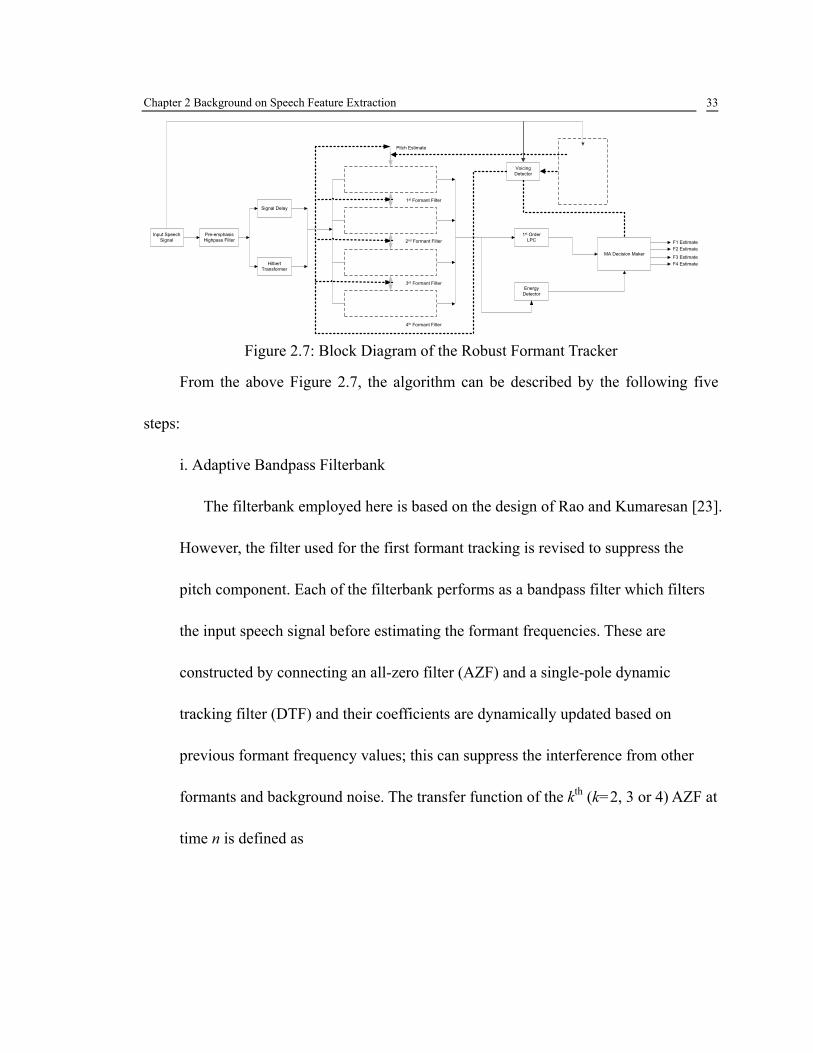
Figure 2.7: Block Diagram of the Robust Formant Tracker
From the above Figure 2.7, the algorithm can be described by the following five
steps:
i. Adaptive Bandpass Filterbank
The filterbank employed here is based on the design of Rao and Kumaresan [23].
However, the filter used for the first formant tracking is revised to suppress the
pitch component. Each of the filterbank performs as a bandpass filter which filters
the input speech signal before estimating the formant frequencies. These are
constructed by connecting an all-zero filter (AZF) and a single-pole dynamic
tracking filter (DTF) and their coefficients are dynamically updated based on
previous formant frequency values; this can suppress the interference from other
formants and background noise. The transfer function of the kth (k=2, 3 or 4) AZF at
time n is defined as

Chapter 2 Background on Speech Feature Extraction 34
[ ]
[ ]( )
[ ] [ ]( )( )∏
∏
≠=
−−−
≠=
−−
−
−
= 4
1
112
4
1
112
1
1
,
kll
nFnFjz
kll
nFjz
AZFkkl
l
er
zer
znHπ
π
, (2.37)
where Fl[n-1] is the formant frequency estimates at the previous time index from
the lth order formant tracker.
Similar to the design of AZF, the coefficients of the DTF in each band is
upgraded to the corresponding formant frequency in previous time index. The
transfer function of the kth DTF at time n is given by
[ ] [ ]( )11211
, −−−−
=zer
rznH nFj
p
pDTFk kπ . (2.38)
ii. Adaptive Energy Detector
The Root-Mean Square (RMS) energy of the signal over the previous 20ms is
calculated for each formant band. The energy threshold is gradually adjusted during
each voiced frame, thus making the algorithm robust to burst loud noises.
iii. Gender Detector
Gender detection is based on the autocorrelation pitch tracking algorithm
discussed in section 2.5.1. The gender G[n] is updated every 20ms, and the speaker
is considered to be male (G[n]=0) if the average pitch frequency is below 180 Hz
and is considered to be female (G[n]=1) if it is great than or equal to 180 Hz.
iv. Voicing Detector
The voice/unvoice detector judges whether the previous frame is voiced or

Chapter 2 Background on Speech Feature Extraction 35
unvoiced. Parameters in each frame such as the common cutoff frequency of the
HPF and LPF and filtered signal’s log energy ratio are adapted slowly to limit the
transient effects. These slowly adapted parameters will make the voicing detector
robust and avoid any sudden changes between voiced and unvoiced frames. For
update equations of each of these parameters, please refer to Kamran’s work [25].
v. Moving Average Decision Maker
The moving average decision maker calculates and updates the value of each
formant frequency according to
[ ] [ ] [ ] [ ]( )( )11002.01 −−−−−= nFnFnFnF iMAiii , (2.39)
where Fi[n] is the formant estimate the ith formant frequency at time n and FiMA[n-1]
is the previous value of the ith formant. Thus, the updated value of each formant
frequency is defined as
[ ] [ ]∑=
=n
kkiMA kF
nnF
1
1 . (2.40)
The algorithm constrains the value of F1, F2, F3 and F4 to be less than 150,
300, 400 and 500 Hz, respectively.
2.7 Pitch-related Features
Prosodic speech features based on fundamental frequency have been used to
identify speaking style and emotional state. Previous studies have shown a high
correlation between such features and the emotional state of the speaker [3]. For instance,

Chapter 2 Background on Speech Feature Extraction 36
sadness has been associated to low standard deviation of pitch and slow speaking rates,
while anger is usually correlated with higher values of pitch deviation and rate. Features
like jitter and shimmer have also been proved helpful in classifying animal arousals as
well as human speech with emotions [2].
In this section, the extraction procedure of two different pitch-related features which
usually employed in emotion and speaking style classification will be introduced. In
Chapter 4, these two features are employed to classify human emotion speech, and
compared with baseline spectral features to demonstrate their functionality.
2.7.1 Jitter
Jitter refers to a short-term (cycle-to-cycle) perturbation in the fundamental
frequency of the voice. Some early investigators such as Lieberman [26] displayed
speech waveforms on oscilloscope and saw that no two periods were exactly alike. The
fundamental frequency appeared “jittery” due to this period variation and the term was
defined as jitter.
The jitter feature of each frame is defined as:
∑=
+−= N
ii
ii
TN
TTJitter
10
100
1, (2.41)
where T0 is the extracted pitch period lengths inμ second.

Chapter 2 Background on Speech Feature Extraction 37
2.7.2 Shimmer
Shimmer was introduced as short term (cycle-to-cycle) perturbation in amplitude by
Wendahl [27]. It is defined as the short term variation in the amplitude of vocal-fold
vibration and perturbation in the amplitude of the voice. Shimmer reflects the transient
change of the utterance’s energy, so it performs as an indicator of different arousal levels.
The shimmer feature of each frame is calculated by
∑=
+−= N
ii
ii
AN
AAShimmer
1
1
1, (2.42)
where Ai is the extracted average amplitude of each speech frame, and N is the number of
extracted pitch periods.
2.8 Log Energy and Delta Features
2.8.1 Log Energy
The log energy of a signal is computed as the log of the speech samples’ energy
with
∑=
=N
nnsE
1
2log . (2.43)
It is normalized by subtracting the maximum value of E in the utterance and adding 1.0,
limiting the energy measure to the range –Emin...1.0.

Chapter 2 Background on Speech Feature Extraction 38
2.8.2 Delta Features
By adding time derivatives to the static features, the classification results of a
speech recognition model can be significantly enhanced. In this research, the delta
coefficients are computed using a standard linear regression formula
∑
∑Θ
=
Θ
=−+ −
=
1
2
1
2
)(
θ
θθθ
θ
θ tt
t
ccd , (2.44)
where dt is a delta coefficient at time t, ct is the corresponding static coefficients; θ is the
configurable window size, set to a value of 2.

Chapter 3 Speech Feature Toolbox Design 39
Chapter 3
3 SPEech Feature Toolbox Design (SPEFT)
Speech toolboxes are widely used in human speech recognition and animal
vocalization research, and can significantly facilitate the feature extraction process.
However, in recent years, with the development of speech feature research, many of the
traditional spectral features such as MFCC and PLP have been extensively modified.
Examples include modifying the frequency warping scale to make the logarithm curve
more concentrated on certain sub-frequency range [28], or changing the perceptual
frequency scaling system. These modifications have generated many new spectral
features like RASTA-PLP, GFCC, and gPLP.
Current toolboxes do not adequately cover any of these modified speech features. In
addition, toolboxes which focus on speech recognition and speaker identification usually
rely on baseline speech features and energy features, often leaving out many alternative
features representing short-term changes in fundamental frequency and energy.
Additionally, the script command based operation handicaps their usage. Moreover,

Chapter 3 Speech Feature Toolbox Design 40
previous works usually do not have batch processing functions, so that extracting
speech features from a large volume of source files is difficult for researchers.
This research focuses on designing a GUI toolbox to cover a wide range of
speech-related features and facilitate speech research for many applications. The
usefulness of the toolbox will be illustrated in Chapter 4 through a speaking style
classification task. In this chapter, the speech feature toolbox design process will be
discussed in detail.
3.1 Review of Previous Speech Toolboxes
Several speech toolboxes have been developed to implement different algorithms in
speech signal processing research, although none are solely designed for extracting
speech features. The most popular ones include the Hidden Markov Toolkit (HTK),
COLEA, and Voice Box; the last two of which are MATLAB toolboxes. Although their
usage in speech research is common, the weaknesses are clear; all of these either lack a
graphic interface for easy access or else do not integrate a wide range of speech features.
3.1.1 Hidden Markov Toolkit (HTK)
HTK is a toolbox for building and manipulating hidden Markov models in speech
recognition and speaker identification research; it is perhaps the most frequently used
toolbox in these fields [29].

Chapter 3 Speech Feature Toolbox Design 41
HTK was first developed by Steve Young at Speech Vision and Robotics Group of
the Cambridge University Engineering Department (CUED) in 1989 and was initially
used for speech recognition research within CUED. In early 1993, as the number of users
grew and maintenance workload increased, the Entropic Research Laboratories (ERL)
agreed to take over distribution and maintenance of HTK. In 1995, HTK V2.0 was jointly
developed by ERL and Cambridge University; this version was a major redesign of many
of the modules and tools in the C library. Microsoft purchased ERL on November 1999,
returned the license to CUED, and the release of HTK became available from CUED’s
website with no cost. [29].
HTK is developed as a speech recognition research platform; although it has been
used for numerous other applications include research in speech synthesis, character
recognition and DNA sequencing. The toolbox integrates multiple algorithms to extract
speech features, including Mel-Frequency Cepstral Coefficients (MFCC), Perceptual
Linear Prediction (PLP) and energy features within each frame; however, due to its
command-line interface and complex operation, it takes hours of study before one can
actually use the toolbox to accomplish a classification task. The feature extraction
procedure would be much easier if these algorithms were integrated into a toolbox with a
GUI interface.
The speech features integrated into HTK are focused on spectral characteristics,
while pitch related features and features like formants are not available. To use additional

Chapter 3 Speech Feature Toolbox Design 42
features for recognition, researchers need to extract those speech features separately
and then use a separate program to convert the data to HTK format and combine them
with the spectral features extracted by HTK itself.
Summary of HTK:
(1) Platform: C
(2) Operation Environment: Command line (Dos/Unix)
(3) Integrated speech features:
MFCC: Mel-frequency Cepstral Coefficients
FBANK: Log Mel-filter bank channel outputs
LPC: Linear Prediction Filter Coefficients
LPREFC: Linear Prediction Reflection Coefficients
LPCEPSTRA: LPC Cepstral Coefficients
PLP: Perceptual Linear Prediction Coefficients
Energy Measures
Delta & Acceleration features
3.1.2 COLEA Toolbox
COLEA is a toolbox developed by Philip Loizou and his research group at the
Department of Electrical Engineering, University of Texas at Dallas [30]. The toolbox is
used as a software tool for speech analysis. Although the toolbox has a GUI interface to

Chapter 3 Speech Feature Toolbox Design 43
operate all of its functions, the integrated features are relatively limited. Only pitch and
formant features can be extracted and plotted. Additionally, it is difficult to export
extracted data from the toolbox. Current speech-related research usually needs to extract
features from a large number of source files for training and testing. Unfortunately, unlike
HTK, the COLEA toolbox does not have batch processing ability to do this. This
limitation to analyze and display only a single file significantly restricts the usability of
the toolbox on a large scale. Figure 3.1 shows the main interface of COLEA toolbox.
Figure 3.1: COLEA toolbox main interface
From an implementation perspective, the toolbox utilizes many global variables,
and the code is not fully commented, making modification or extensive work on the
toolbox relatively difficult.
Summary of COLEA:
(1) Platform: MATLAB
(2) Interface: GUI interface

Chapter 3 Speech Feature Toolbox Design 44
(3) Integrated speech features:
Energy Contour
Power Spectral Density
Pitch Tracking
Formant (First three orders)
3.1.3 Voice Box
Voice Box is a speech processing toolbox which integrates multiple speech
processing algorithms on MATLAB platform. It is designed and maintained by Mike
Brookes, Department of Electrical & Electronic Engineering at Imperial College, United
Kingdom [31].
Voice Box provides a series of functions for speech analysis and speech recognition;
however, the number of speech features it integrates are limited and consists solely of
stand-alone MATLAB functions, so extra coding work is needed when applying this
toolbox to batch process a large number of source files for specific speech research.
Summary of Voice Box:
(1) Platform: MATLAB
(2) Interface: MATLAB function command
(3) Integrated speech features:
LPC Analysis

Chapter 3 Speech Feature Toolbox Design 45
Pitch Tracking
Mel-Frequency Cepstral Coefficients
Filter Bank Energy
Zero-crossing rate
3.2 MATLAB Graphical User Interface (GUI) Introduction
A graphical user interface (GUI) is a graphical display that contains devices, or
components, that enable a user to perform interactive tasks. To perform these tasks, the
user of the GUI does not have to create a script or type commands at the command line.
A well designed GUI can make programs easier to use by providing them with consistent
appearances and convenient controls. The GUI components can be menus, toolbars, push
buttons, radio buttons, list boxes, and sliders. Each component is associated with one or
more user defined routines known as callback functions. The execution of each callback
is triggered by a particular user action such as a button push, mouse click, selection of a
menu item, or the cursor passing over a component.
In SPEFT’s GUI design, the MATLAB platform is selected since there is a large
volume of open source code of various speech feature algorithms online, which makes
the extensive work easier. Moreover, the platform itself is the most commonly used one
in speech research.
There are three principal elements required to create a MATLAB Graphical User

Chapter 3 Speech Feature Toolbox Design 46
Interface [32]:
(1) Components: Each objects displayed on a MATLAB GUI (pushbuttons,
checkboxes, toggle buttons, lists, etc.), static elements (frames and text strings),
menus and axes.
(2) Figures: The components of a GUI must be arranged within a figure window.
(3) Callbacks: Routines that are executed whenever the user activates the component
objects. Both MATLAB scripts and functions can be compiled as callback
routines. Each graphical component on GUI has a corresponding callback routine.
Components employed in SPEFT include Push Buttons, Check Boxes, Popup
Menus, Edit Boxes, Menu items, Frames, Radio Buttons and Axes. Properties of these
objects such as Position, Font Size, Object Tag and Visibility are controlled by MATLAB
command “uicontrol”. For detailed description of these objects, please refer to MATLAB
instruction [32].
3.3 SPEech Feature Toolbox (SPEFT) Design
3.3.1 GUI Layout
Once the toolbox is installed, it can be launched by typing “SPEFT” in the
MATLAB command window. The main window interface is shown in Figure 3.2.

Chapter 3 Speech Feature Toolbox Design 47
Figure 3.2: GUI Layout of the Main Interface
The objects displayed on the main interface are sub-grouped into four regions; each
of which represents a certain category. This design gives the user a clear overview of the
integrated functions in SPEFT, and provides easier operation when extracting features.
The four object groups are:
(1) File operation buttons: Displayed in the upper left corner, this is used for loading
single files and launching the batch process interface.
(2) Signal display axes and information bar: Displayed in the middle of the main
interface, this is used for displaying signal information in single file mode and
basic signal operations.
(3) Feature selection check boxes and parameter configuration buttons: This is
displayed below the main signal axes. By selecting the check boxes next to those

Chapter 3 Speech Feature Toolbox Design 48
push buttons tagged with feature’s names, user can extract features in different
combinations. The parameters of each speech feature extraction algorithm are
given default values and can be configured independently.
(4) Extraction button: Displayed on the right bottom corner, this is used for starting
the feature extraction process.
Each parameter is given default value. Users can modify each parameter through
operating each feature’s parameter configuration interface. Figure 3.3 and Figure 3.4
show the parameter configuration interface for MFCC and LPC features.
Figure 3.3: MFCC Parameter Configuration Interface GUI Layout

Chapter 3 Speech Feature Toolbox Design 49
Figure 3.4: LPC Parameter Configuration Interface GUI Layout
3.3.2 Batch Processing Mode
Speech recognition research usually requires extracting speech features from
hundreds or even thousands of source files. To facilitate this process, SPEFT integrates
the batch process function which can extract multiple speech features from a large
volume of source files. The Batch processing interface is displayed in Figure 3.5.

Chapter 3 Speech Feature Toolbox Design 50
Figure 3.5: Batch File Processing Interface Layout
Users can select the source directory and destination directory where the speech
source files and exported features are stored, respectively. Once the batch process is
started, SPEFT recursively searches the entire source directory and its sub-directories.
For those SPEFT supported files, the features are extracted and exported to the
destination directory in HTK format files, while files in other formats allow users to
select whether to copy directly from source folder to destination folder. Users can also
specify the extension of the exported feature files. The source directory’s hierarchical
structure is kept the same in the destination directory.
3.3.3 Hierarchical Feature with Different Window Size
To improve speech recognition accuracy, speech researchers frequently combine

Chapter 3 Speech Feature Toolbox Design 51
different speech features together. However, the nature of frame-based feature
processing necessitates one feature vector per frame, regardless of feature type. Some
types of features require a larger window size. This problem usually makes feature
combination difficult with current toolboxes.
In SPEFT, parameters, including window sizes of each speech feature, are
independently configured, and the user may extract features using different window sizes.
SPEFT applies a unified step size across all user selected features. As previously
discussed in Section 2.3, the traditional framing method usually takes the first point of a
signal as the starting point for framing. Assuming an input signal with a total of N
samples, a window length of l and a step size of m, the total number of frames is
mmlNN frames
)( −−= , (3.1)
and the ith frame is centered at
)1(2
−+= imlCenteri . (3.2)
When the window size l is changed, the center point of each frame also changed.
By employing a fixed step size framing method, the original signal is zero-padded
both at the beginning and the end. Thus, the ith frame is centered at
)1(2
' −+= immCenteri . (3.3)
The center of each frame is only determined by the step size. Thus, no matter how the
window size changed over different features, the length of extracted feature vectors are
still consistent.
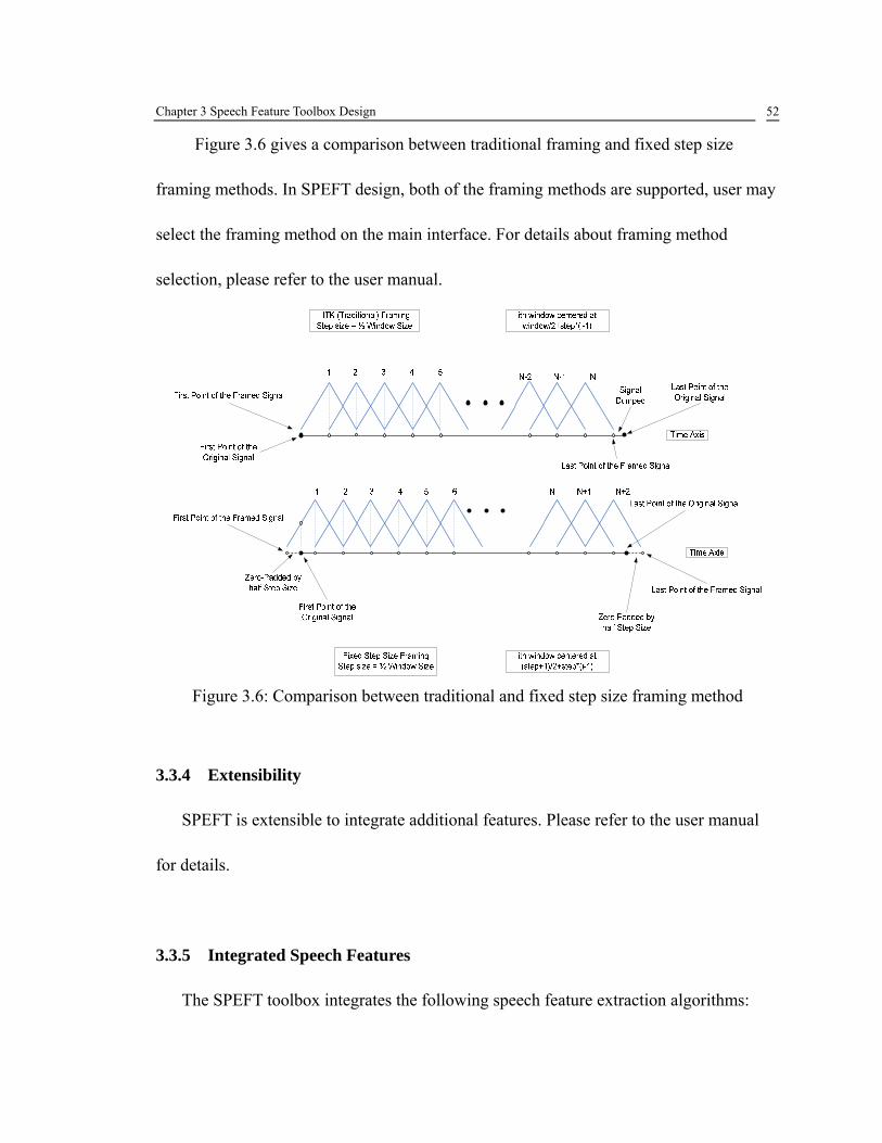
Chapter 3 Speech Feature Toolbox Design 52
Figure 3.6 gives a comparison between traditional framing and fixed step size
framing methods. In SPEFT design, both of the framing methods are supported, user may
select the framing method on the main interface. For details about framing method
selection, please refer to the user manual.
Figure 3.6: Comparison between traditional and fixed step size framing method
3.3.4 Extensibility
SPEFT is extensible to integrate additional features. Please refer to the user manual
for details.
3.3.5 Integrated Speech Features
The SPEFT toolbox integrates the following speech feature extraction algorithms:

Chapter 3 Speech Feature Toolbox Design 53
(1) Spectral Features:
MFCC: Mel-Frequency Cepstral Coefficients;
GFCC: Greenwood-Frequency Cpestral Coefficients;
PLP: Perceptual Linear Prediction Coefficients;
gPLP: generalized Perceptual Linear Prediction Coefficients;
RASTA-PLP: RelAtive SpecTraAl (RASTA)-PLP;
LPC: Linear Prediction Filter Coefficients;
LPREFC: Linear Prediction Reflection Coefficients;
LPCEPSTRA: LPC Cepstral Coefficients;
FBANK: Log Mel-filter bank channel output ;
Delta & Acceleration features;
(2) Pitch Tracking Algorithms:
Autocorrelation Pitch Detection;
Cepstrum Pitch Detection;
Average Magnitude Difference Function (AMDF);
Robust Algorithm for Pitch Tracking (RAPT)
(3) Formant Tracking Algorithms:
Formant estimation by LPC root-solving procedure;
Formant estimation by Dynamic Tracking Filter (DTF);
(4) Features used in speaking style classification:

Chapter 3 Speech Feature Toolbox Design 54
Jitter;
Shimmer;
Sub-harmonic to Harmonic Ratio;
(5) Other features:
Zero-crossing-rate;
Log Energy;
For the controllable parameters of each speech feature, please refer to the SPEFT
manual.

Chapter 4 Speaking Style Classification Using SPEFT 55
Chapter 4
4 Speaking Style Classification Using SPEFT
In this chapter, a speaking style classification experiment is implemented. All
speech features are extracted by both SPEFT and HTK, using the Speech Under
Simulated and Actual Stress (SUSAS) dataset. The goal is to demonstrate the feature
extraction process and effectiveness of SPEFT compared to an existing toolbox.
Extracted speech features include baseline spectral features, particularly the
Mel-frequency Cepstral Coefficients (MFCCs) and log energy. These are combined with
the two pitch-related speech features jitter and shimmer, introduced in section 2.5.1 and
2.5.2.
Extracted features are reformatted and written into HTK file format. The HMM
classifier in HTK is applied to these combined feature vectors, with the observation
probability at each state represented by Gaussian Mixture Models (GMMs).
The classification results using different feature combinations are compared to
demonstrate the effectiveness of jitter and shimmer features in classifying human speech
with various speaking styles. The detailed parameter configurations for each feature

Chapter 4 Speaking Style Classification Using SPEFT 56
extraction are also provided.
4.1 Introduction
The classification of different speaking styles, stresses and emotions has become
one of the latest challenges in speech research in recent years [2, 3, 33]. This task has
applications to a number of important areas, including security systems, lie detection,
video games and psychiatric aid, etc. The performance of emotion recognition largely
depends on successful extraction of relevant speaker-independent features. Previous work
has been conducted to investigate acoustic features in order to detect stress and emotion
in speech and vocalizations based on HMMs [34], and to examine the correlation
between certain statistical measures of speech and the emotional state of the speaker [28].
The most often considered features include fundamental frequency, duration, intensity,
spectral variation and log energy. However, many of these features are typically
discriminatory across a subset of possible speaking styles, so that systems based on a
small feature set are unable to accurately distinguish all speaking styles. Improvement in
accuracy can be achieved by adding additional features related to measures of variation in
pitch and energy contours.
Two such recently investigated acoustic features are jitter and shimmer. Fuller et al.
found increased jitter to be an “indicator of stressor-provoked anxiety of excellent
validity and reliability” [35], and both jitter and shimmer can be indicators of underlying

Chapter 4 Speaking Style Classification Using SPEFT 57
stress in human speech.
In addition, to evaluate the effectiveness and accuracy of the SPEech Feature
Toolbox (SPEFT) compared to previous toolboxes, speech features are extracted by both
SPEFT and HTK. A HMM classifier is applied to discriminate different speaking styles
with the above two sets of features.
4.2 Experiment Outline
4.2.1 SUSAS Database
The Speech Under Simulated and Actual Stress (SUSAS) dataset was created by the
Robust Speech Processing Laboratory at the University of Colorado-Boulder [30]. The
database encompasses a wide variety of stresses and emotions. Over 16,000 utterances
were generated by 32 speakers with their ages ranging from 22 to 76. Utterances are
divided into two domains, “actual” and “simulated”. In this classification task, only the
simulated utterances are employed. The eleven styles include Angry, Clear, Cond50,
Cond70, Fast, Lombard, Loud, Neutral, Question, Slow and Soft. The Cond50 style is
recorded with the speaker in a medium workload condition, while in the Cond70 style the
speaker is in a high workload condition. The Lombard speaking style contains utterances
from subjects listening to pink noise presented binaurally through headphones at a level
of 85 dB.

Chapter 4 Speaking Style Classification Using SPEFT 58
Table 4.1: Summary of the SUSAS Vocabulary
The vocabulary of each speaking style includes 35 highly confusable aircraft
communication words which are summarized in Table 4.1. Each of the nine speakers (3
speakers from each of the 3 dialect regions) in the dataset has two repetitions of each
word in each style. All speech utterances were sampled by 16 bits A/D converter at a
sample frequency of 8 kHz. For more information about SUSAS dataset, refer to Hansen
et al. [30].
4.2.2 Acoustic Models
In this research, a Hidden Markov Model (HMM) approach is used to classify
human speech with different speaking styles. HMMs are the most common statistical
classification model for speech recognition and speaker identification [36]. Compared to
other statistical analysis such as Artificial Neural networks (ANN), HMMs have the
ability of non-linearly aligning speech models and waveforms while allowing more
complex language models and constraints [34, 37].
SUSAS VOCABULARY LIST
break eight go nav six thirty change enter hello no south three degree fifty help oh stand white hot fix histogram on steer wide east freeze destination out strafe zero eight gain mark point ten

Chapter 4 Speaking Style Classification Using SPEFT 59
State 2
State 3
State 4
State1
State5
a12 a23 a34a45
a22 a33 a44
b1(• ) b2(• ) b3(• )
Speech Feature Distributionat Each state
State Probability at each frame
Choose Max
P(O|M1) P(O|M2) P(O|M3)
Trained Model
Extracted Features from Training Data
Figure 4.1: HMM for Speech Recognition
A silence model labeled with “sil” is inserted both at the beginning and end of each
utterance to correspond to the silent region introduced in recording, followed by the
appropriate speaking style model. Both the “sil” and speaking style labels are represented
by a three-state HMM. Thus, each of the utterances in SUSAS dataset is modeled with a
sequence of three HMMs. Figure 4.1 displays an example of one such HMM.
HMMs are finite-state machines, with transitional probabilities aij between states i
and j, coupled with observation probabilities bj(·) at each specific state. Given a model λ,
an observation sequence O = {O1, O2, O3,…, OT} and initial value πi, then the Viterbi
dynamic programming algorithm is used for recognition. Viterbi recognition finds the

Chapter 4 Speaking Style Classification Using SPEFT 60
state sequence with the highest likelihood in a given model.
The observation probability bj(·) is usually represented by Gaussian Mixture
Models (GMMs), which are weighted sums of multivariate Gaussian distributions. The
emitted GMMs observation probability at time t in state j is given by
∑=
Σ=M
mtjmjmjmtj ONcOb
1, );()( μ , (4.1)
where M is the number of mixture components, cjm is the weight of the m’th component
and N(μ, Σ; O) is a multivariate Gaussian with μ as the mean vector and Σ as the
covariance matrix. In this research, the observation probability at each state is represented
by a four GMM mixture model.
Given training data, the maximum likelihood estimates of j
∧
μ and j
∧
Σ is estimated
using Baum-Welch re-estimation.
4.3 Speech Feature Extraction Process
Speech features employed in this experiment include Mel-frequency Cepstral
Coefficients (MFCCs), jitter, shimmer and Energy with their first and second order delta
features. The extraction procedures of these features are introduced in section 2.4.1, 2.7.1,
2.7.2 and 2.8 respectively. The cepstrum pitch detection algorithm discussed in section
2.3.2 was employed to determine the pitch frequency when extracting jitter features. It
also serves as the voiced/unvoiced detector.
To verify the effectiveness of the two pitch-related features jitter and shimmer in

Chapter 4 Speaking Style Classification Using SPEFT 61
speaking style classification, the above four speech features were extracted in different
combinations. Table 4.2 gives the numbers of each feature extracted from each speech
frame.
Table 4.2: Speech Features Extracted from Each Frame
The HTK’s “config” file setup is listed below for complete description of parameter
settings. Note that TARGETKIND may vary when extracting different features types:
# Coding Parameters SOURCEKIND = WAVEFORM SOURCEFORMAT = WAV TARGETKIND = MFCC_E_D_A TARGETRATE = 100000 WINDOWSIZE = 300000 SAVECOMPRESSED = F SAVEWITHCRC = F USEHAMMING = T PREEMCOEF = 0.97 NUMCHANS = 26 CEPLIFTER = 22 NUMCEPS = 24 ENORMALISE = T
To keep the parameter configurations consistent, the feature configuration interfaces
in SPEFT are displayed in Figure 4.2.
Feature Name
MFCCs
MFCCs Delta
MFCCs D-D
Energy
Energy Delta
Energy D-D
Jitter
Shimmer
Total
Mel+E 24 24 24 1 1 1 0 0 75 Mel+E
+J 24 24 24 1 1 1 1 0 76
Mel+E+S
24 24 24 1 1 1 0 1 76
Mel+E+J+s
24 24 24 1 1 1 1 1 77

Chapter 4 Speaking Style Classification Using SPEFT 62
Figure 4.2: Jitter Parameter Configurations in SPEFT
Figure 4.3: Shimmer Parameter Configurations in SPEFT

Chapter 4 Speaking Style Classification Using SPEFT 63
Figure 4.4: MFCCs Parameter Configurations in SPEFT
Figure 4.5: Energy Parameter Configurations in SPEFT

Chapter 4 Speaking Style Classification Using SPEFT 64
4.4 Speaking Style Classification Based on SUSAS
In order to validate the SPEFT toolbox and the effectiveness of jitter and shimmer
features, speech features were extracted using both the SPEFT toolbox and HTK plus
MATLAB calculation. Of the eleven speaking styles labeled in the SUSAS dataset, six
emotion-related speaking styles are selected for the classification study (the remainders
are considered to be related to noise conditions rather than speaking style). These include
Angry, Fast, Lombard, Question, Slow and Soft. Training and testing is implemented
through a three-fold cross-validation scheme within each dialect type, so that the results
are speaker independent but dialect dependent. This results in training sets of 140
utterances per speaking style and corresponding testing sets of 70 utterances. The average
accuracy value across the three folds in each dialect type was used to determine the
overall accuracy. Four different combinations of speech features were extracted from
SUSAS dataset and they are listed in Table 4.2.
To validate the SPEFT toolbox, the parameter configurations are unified between
SPEFT and HTK, except for the framing method, since SPEFT employs a fixed step size
method. The window size is set to 30ms with a 10ms step size in feature extraction. The
parameters configuration interfaces are displayed in Figure 4.2 to Figure 4.5.
Three-state left-to-right HMMs with four-mixture GMMs in each state are used for
classification models. The programming toolkit HTK 3.2.1 from Cambridge University
[38] is used for all training and testing.

Chapter 4 Speaking Style Classification Using SPEFT 65
4.5 Experiment Results and Discussion
In order to verify the accuracy of SPEFT toolbox and prove the effectiveness of
jitter and shimmer features in speaking style classification, speech features are extracted
by both SPEFT and HTK. These features are used in two experiments and their results
are compared below:
1) SPEFT toolbox verification:
MFCCs + Energy features extracted by both SPEFT and HTK toolbox
are employed to an HMM classifier to classify the speaking styles. The
classification results are compared in Figure 4.6 and Table 4.3. There is a
slight difference between the classification results of these two sets of
features. The SPEFT’s average classification result over all six speaking
styles is slightly higher than HTK by 1%.
In Chapter 5, the accuracy of the speech features themselves, as
extracted by SPEFT, will be tested against other toolboxes.
2) Effectiveness of jitter and shimmer features:
The classification results using feature vectors with and without jitter
and shimmer are compared in Figure 4.7 and Table 4.4. Compared to the
baseline spectral features; the results are improved by 2.09%, 3.10% and
3.55% with jitter, shimmer and both are included, respectively.
Jitter and shimmer features have also been extracted from African elephant

Chapter 4 Speaking Style Classification Using SPEFT 66
(Loxodonta Africana) and Rhesus monkey (Macaca mulatta) vocalizations to classify
the animal’s emotional arousal level. By combining with GFCCs discussed in section
2.2.1, the classification results showed a unified improvement. For details of the animal’s
emotional arousal classification, please refer to Xi Li et al [2].
4.6 Conclusions
The differences of classification results between features extracted from SPEFT and
HTK are in a reasonable range. The difference mainly comes from the different framing
method between SPEFT and HTK.
Jitter and shimmer features have been evaluated as important features for analysis
and classification of speaking style in human speech. Adding jitter and shimmer to
baseline spectral and energy features in an HMM-based classification model resulted in
increased classification accuracy across all experimental conditions.
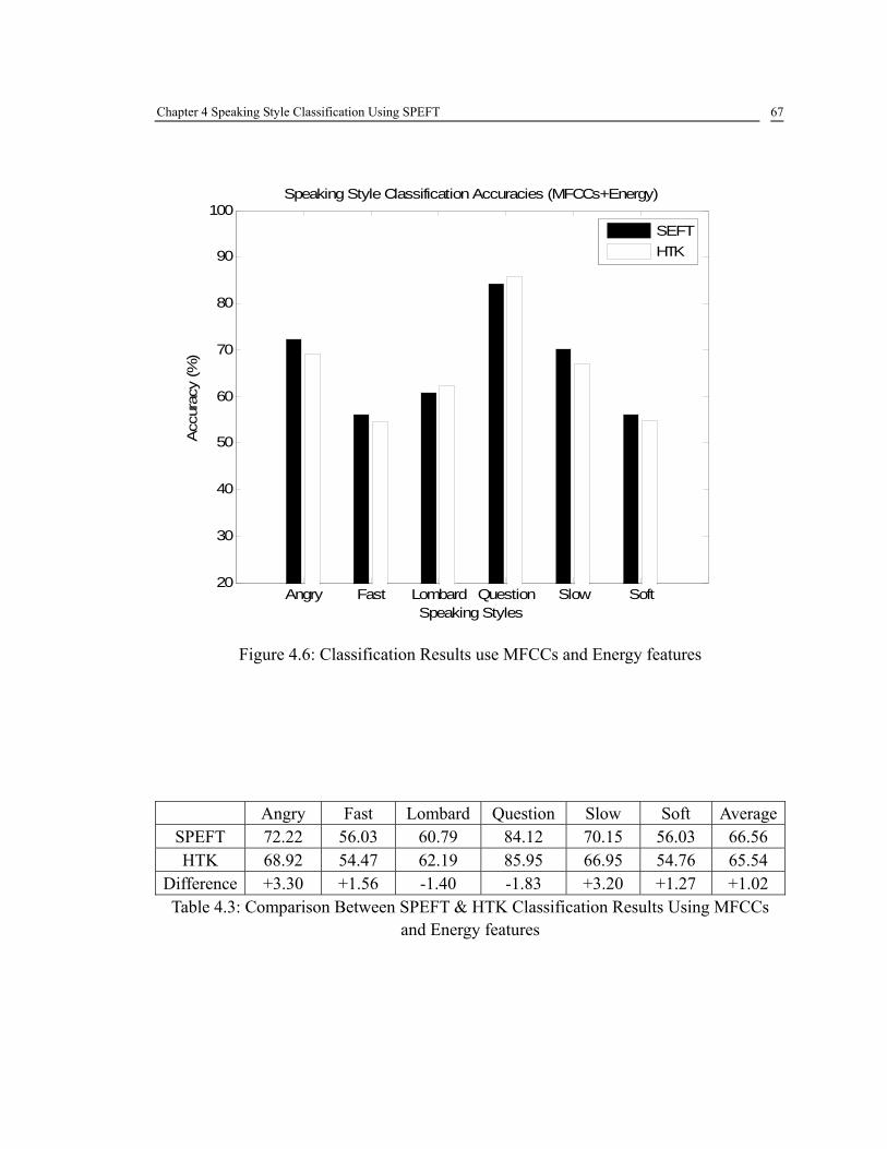
Chapter 4 Speaking Style Classification Using SPEFT 67
Angry Fast Lombard Question Slow Soft20
30
40
50
60
70
80
90
100
Speaking Styles
Acc
urac
y (%
)Speaking Style Classification Accuracies (MFCCs+Energy)
SEFTHTK
Figure 4.6: Classification Results use MFCCs and Energy features
Angry Fast Lombard Question Slow Soft AverageSPEFT 72.22 56.03 60.79 84.12 70.15 56.03 66.56 HTK 68.92 54.47 62.19 85.95 66.95 54.76 65.54
Difference +3.30 +1.56 -1.40 -1.83 +3.20 +1.27 +1.02 Table 4.3: Comparison Between SPEFT & HTK Classification Results Using MFCCs
and Energy features

Chapter 4 Speaking Style Classification Using SPEFT 68
Angry Fast Lombard Question Slow Soft20
30
40
50
60
70
80
90
100
Speaking Styles
Acc
urac
y (%
)Speaking Style Classification Accuracies
Mel+EMel+E+JMel+E+SMel+E+J+S
Figure 4.7: Classification Results by Combining Baseline
Features and Pitch-related Features
Angry Fast Lombard Question Slow Soft AverageMel+E 68.92 54.47 62.19 85.95 66.95 54.76 65.54
Mel+E+J 70.66 56.43 62.52 86.43 67.52 62.24 68.05 Mel+E+S 70.24 55.24 65.81 86.19 74.33 60.05 68.64
Mel+E+J+S 72.24 55.67 68.66 86.67 69.19 62.09 69.09 Table 4.4: HTK Classification Results Using Different Feature Combinations

Chapter 5 SPEFT Testing 69
Chapter 5
5 SPEFT Testing
In this chapter, the reliability of SPEFT toolbox is tested through a standard testing
dataset. The features extracted by SPEFT are compared to those extracted by existing
toolboxes including HTK, COLEA and Voice Box. The distance between feature vectors
are measured to evaluate the reliability of SPEFT.
5.1 Software Testing Basics
Software testing, or software verification and validation (V & V) is intended to
show that a software system conforms to its specification and that the system meets the
expectations of its user. It involves checking processes, such as inspections and reviews,
at each stage of the software process from user requirements definition to program
development [39].

Chapter 5 SPEFT Testing 70
Component Testing
System Testing
Acceptance Testing
Figure 5.1: Testing Process
Except for small programs, systems should not be tested as a single unit. Figure 5.1
shows a three-stage testing process where system components are tested, the integrated
system is tested and the system is tested with the example dataset. Ideally, component
defects are discovered early in the process and interface problems when the system is
integrated. As defects are discovered, the program must be debugged.
Requirements Specification
System Specification
System Design
Detailed Design
Acceptance Test Plan
System Integration Test Plan
Sub-system Integration Test Plan
Module and Unit Code and Test
Acceptance Test
System Integration
Test
Sub-system Integration
TestService
Figure 5.2: Testing Phases in Software Process
The three stages involved in testing process are:
(1) Component Testing
Individual components are tested to ensure that they operate correctly. Each

Chapter 5 SPEFT Testing 71
component is tested independently, without other system components.
Components may be simple entities such as functions or object classes, or may be
groups of these entities.
In SPEFT testing, this stage is achieved by independently testing the
functionality of each feature’s extraction program.
(2) System Testing
The components are integrated to make up the system. This process is
concerned with finding errors that result from unanticipated interactions between
components and component interface problems. It is also concerned with
validating that the system meets its functional and non-functional requirements
and testing the emergent system properties.
In this research, this stage is completed by testing the overall performance of
SPEFT, including extracting multiple speech features in both single file and batch
mode.
(3) Acceptance Testing
This is the final stage in the testing process before the system is accepted for
operational use. The system is tested with data supplied by the system customer
rather than with simulated test data. Acceptance testing may reveal errors and
omissions in the system requirements definition because the real data exercise the
system in different ways from the test data. Acceptance testing may also reveal

Chapter 5 SPEFT Testing 72
requirements problems where the system’s facilities do not really meet the user’s
needs or the system performance is unacceptable. It is sometimes called alpha
testing.
In SPEFT testing, this stage is completed by creating a verification dataset and
setting a series of thresholds to test the distance between feature matrices extracted
by SPEFT and current existing toolboxes.
5.2 Standard Testing Data
To test the SPEFT toolbox, eleven speech utterances are collected from the
following three speech databases:
(1) TIMIT Speech Database
The TIMIT speech database was designed to provide acoustic phonetic speech
data for the development and evaluation of automatic speech recognition systems. It
contains a total of 6300 sentences collected from 630 speakers from 8 dialect
regions of America, each speaking 10 sentences. The utterances in the TIMIT
database are sampled at 16 kHz.
In addition to each utterance’s waveform file, three associated transcription
files (.txt, .wrd, .phn) are included in the TIMIT corpus. In these three files, the .txt
file associates the prompt of the words the speaker said; the .wrd file stores the
time-aligned word transcription, and the .phn file stores the time-aligned phonetic

Chapter 5 SPEFT Testing 73
transcriptions of each utterance.
In this testing research, four utterances labeled as “SI747.wav”, “SI1377.wav”,
“SI631.wav” and “SI1261.wav” are selected from TIMIT dataset. Transcripts of
these files are listed below.
SI1377: “As these maladies overlap, so must the cure”. (Female)
SI1261: “In two cases, airplanes only were indicated”. (Male)
SI631: “Program notes reads as follows: take hands; this urgent visage
beckons us”. (Male)
SI747: “Add remaining ingredients and bring to a boil”. (Female)
(2) SUSAS Dataset
This dataset has been introduced in section 4.2.1. In this experiment, three
utterances are selected from “GENERAL” dialect with a male speaker speaking the
word “BREAK”, “EIGHTY” and “OUT”.
(3) Aurora Project Database
This corpus contains utterances connected English digits embedded in
additive noise as well as the clean speech. Background noise including several types
of artificially created distortion environments with a range of SNR from -5 to 20 dB.
Four utterances are selected from the AURORA2 database[40]. All four selected
utterances are clean speech. File names and transcripts are listed below:
FRL_9Z9A: “Nine zero nine”; (Female)
Chapter 5 SPEFT Testing 74
FRL_OOA: “Oh, oh”; (Female)
MAH_3A: “Three”; (Male)
MAH_139OA: “One three nine oh”. (Male)
5.3 Testing Method
To evaluate the accuracy of SPEFT toolbox, a validation test is carried out in this
section. Speech features are extracted by both SPEFT and well recognized toolboxes
including HTK, COLEA and Voice Box. Both experiments are given consistent parameter
configurations. The features calculated by existing toolboxes and SPEFT are defined as
standard data and testing data, respectively. The distance between standard feature
vectors and testing feature vectors are computed to evaluate the overall difference.
Given two N dimension vectors, with X as the standard vector and Y as the testing
vector, the following two measures of error between these two vectors are computed:
(1) Mean Square Error (MSE):
∑=
−=N
iiiMSE yx
NE
1
21 , (5.1)
(2) Mean Percentage Error (MPE):
%10011
×−
= ∑=
N
i i
iiMPE x
yxN
E , (5.2)
where xi is the ith element in vector X.
Thus, given a speech utterance with M frames and N features computed in each

Chapter 5 SPEFT Testing 75
frame, an M×N feature matrix can be extracted constructed by existing toolboxes and
SPEFT as standard and testing feature matrix, respectively. The overall error between
these two matrices by employing MSE and MPE are:
(1) mean MSE (mMSE):
∑ ∑∑= ==
⎟⎠
⎞⎜⎝
⎛−==
M
j
N
iijij
M
jMSEjmMSE yx
NME
ME
1 1
2
1
111 , (5.3)
where EMSEj is the Mean Square Error between jth frame’s feature vector and xij is
the ith feature in the jth frame of the standard matrix;
(2) mean MPE (mMPE):
∑ ∑∑= == ⎟
⎟
⎠
⎞
⎜⎜
⎝
⎛×
−==
M
j
N
i ij
ijijM
jMPEjmMPE x
yxNM
EM
E1 11
%100111 , (5.4)
where EMPEj is the Mean Square Error between jth frame’s feature vector.
5.4 Testing Experiments
5.4.1 System Testing
The system is tested by batch extracting features from the standard dataset. This
experiment can be validated by using SPEFT to extract different speech features, since
each of the feature implementations is considered a separate component in the SPEFT
system. An example of system testing was given in Chapter 4, since the experiment
employed multiple speech features (MFCCs, Energy, jitter, shimmer and their 1st and 2nd
delta features).

Chapter 5 SPEFT Testing 76
5.4.2 Component Testing
Speech feature vectors extracted by SPEFT are compared to those extracted by
other toolboxes. The distances and percent difference are calculated using Equation 5.3
and 5.4. The result reflects the functionality and accuracy of each component.
5.4.3 Acceptance Testing
The computed distances are further processed to compute the average distance and
percent difference. If the percent difference exceeds a certain amount, the result is
rejected.
5.5 Testing Results
5.5.1 MFCCs
The MFCCs are extracted from the standard dataset by employing both SPEFT and
HTK. In the SPEFT design, the programs used to extract MFCC features are modified
from the implementation of Ellis [41]. The fixed step sized framing method is employed
when calculating the power spectrum in each frame in SPEFT. To ensure the input signal
is consistent in both the toolboxes, the dataset is zero-padded before being passed into
HTK, so that the frames are exactly aligned for comparison.
In HTK the setup of the “config” file is listed below:
# Coding Parameters SOURCEKIND = WAVEFORM

Chapter 5 SPEFT Testing 77SOURCEFORMAT = WAV TARGETKIND = MFCC_D TARGETRATE = 100000 WINDOWSIZE = 300000 USEHAMMING = T PREEMCOEF = 0.97 NUMCHANS = 20 CEPLIFTER = 22 NUMCEPS = 12
To make the parameter configurations consistent, the feature configuration interface
in SPEFT is displayed in Figure 5.3:

Chapter 5 SPEFT Testing 78
Figure 5.3: MFCC Parameter Configuration Interface in SPEFT

Chapter 5 SPEFT Testing 79
Testing results are listed in Table 5.1:
File Name Row No. Window No. mMSE mMPE (%)
BEAK1.wav 24 52 0.0026 2.1470
EIGHTY1.wav 24 47 0.0027 2.4002
FRL_9Z9A.wav 24 169 0.0043 3.5397
FRL_OOA.wav 24 134 0.0041 3.4438
MAH_139OA.wav 24 147 0.0044 3.0339
MAH_3A.wav 24 81 0.0042 3.0977
MSI1261.wav 24 273 0.0031 2.4197
SI1261.wav 24 514 0.0032 2.4981
SI631.wav 24 46 0.0033 2.5274
OUT1.wav 24 387 0.0037 2.7204
SI1377.wav 24 303 0.0038 2.4651
Average - - 0.0036 2.7539
Table 5.1: MFCC Test Results
5.5.2 PLP
The PLPs are extracted from the standard dataset by employing both SPEFT and
HTK. In SPEFT design, the programs used to extract PLP features are modified from the
implementation of Ellis [41]. The fixed step sized framing method is employed when

Chapter 5 SPEFT Testing 80
calculating the power spectrum in each frame. In HTK the “config” file setup is listed
below:
# Coding Parameters SOURCEKIND = WAVEFORM SOURCEFORMAT = WAV TARGETKIND = PLP TARGETRATE = 100000 WINDOWSIZE = 300000 USEHAMMING = T PREEMCOEF = 0.97 NUMCHANS = 20 CEPLIFTER = 22 NUMCEPS = 12 USEPOWER = T LPCORDER = 12
To make the parameter configurations consistent, the PLP parameter configuration
interface in SPEFT is displayed in Figure 5.4:

Chapter 5 SPEFT Testing 81
Figure 5.4: PLP Parameter Configuration Interface in SPEFT

Chapter 5 SPEFT Testing 82
Test results are listed in Table 5.2:
File Name Row No. Window No. mMSE mMPE (%)
BEAK1.wav 24 52 0.0038 5.1606
EIGHTY1.wav 24 47 0.0054 6.6130
FRL_9Z9A.wav 24 169 0.0034 6.1264
FRL_OOA.wav 24 134 0.0053 7.1830
MAH_139OA.wav 24 147 0.0034 5.5479
MAH_3A.wav 24 81 0.0036 6.6573
MSI1261.wav 24 273 0.0051 6.2559
SI1261.wav 24 514 0.0047 6.5116
SI631.wav 24 46 0.0045 4.5864
OUT1.wav 24 387 0.0056 5.4080
SI1377.wav 24 303 0.0052 5.2816
Average - - 0.0046 5.9392
Table 5.2 PLP Test Results
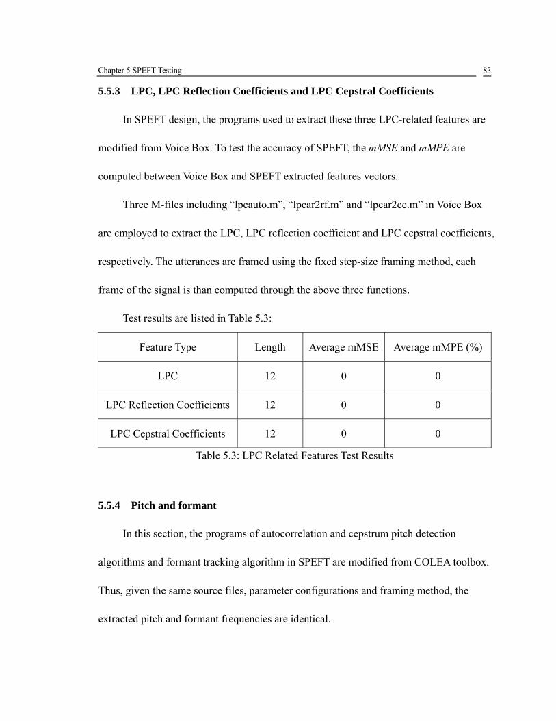
Chapter 5 SPEFT Testing 83
5.5.3 LPC, LPC Reflection Coefficients and LPC Cepstral Coefficients
In SPEFT design, the programs used to extract these three LPC-related features are
modified from Voice Box. To test the accuracy of SPEFT, the mMSE and mMPE are
computed between Voice Box and SPEFT extracted features vectors.
Three M-files including “lpcauto.m”, “lpcar2rf.m” and “lpcar2cc.m” in Voice Box
are employed to extract the LPC, LPC reflection coefficient and LPC cepstral coefficients,
respectively. The utterances are framed using the fixed step-size framing method, each
frame of the signal is than computed through the above three functions.
Test results are listed in Table 5.3:
Feature Type Length Average mMSE Average mMPE (%)
LPC 12 0 0
LPC Reflection Coefficients 12 0 0
LPC Cepstral Coefficients 12 0 0
Table 5.3: LPC Related Features Test Results
5.5.4 Pitch and formant
In this section, the programs of autocorrelation and cepstrum pitch detection
algorithms and formant tracking algorithm in SPEFT are modified from COLEA toolbox.
Thus, given the same source files, parameter configurations and framing method, the
extracted pitch and formant frequencies are identical.

Chapter 5 SPEFT Testing 84
5.5.5 Energy
The energy feature in each frame of signal is extracted from the standard dataset by
employing both SPEFT and HTK.
Due to the design of HTK, energy feature cannot be extracted separately. Thus, it
is computed along with MFCC features. The “config” file setup is listed below:
# Coding Parameters SOURCEKIND = WAVEFORM SOURCEFORMAT = WAV TARGETKIND = MFCC_E TARGETRATE = 100000 WINDOWSIZE = 300000 USEHAMMING = T PREEMCOEF = 0.97 NUMCHANS = 20 CEPLIFTER = 22 NUMCEPS = 8 ENORMALISE = T ZMEANSOURCE = T

Chapter 5 SPEFT Testing 85
To make the parameter configurations consistent, the Energy configuration interface
in SPEFT is displayed in Figure 5.5:
Figure 5.5: Energy Parameter Configuration Interface in SPEFT

Chapter 5 SPEFT Testing 86
Two sets of energy features are compared with the “Normalize” switch turned on
and off, respectively.
Test results are listed in Table 5.4 and Table 5.5:
File Name Row No. Window No. mMSE mMPE (%)
BEAK1.wav 1 52 0.0000 1.1637
EIGHTY1.wav 1 47 0.0000 0.1399
FRL_9Z9A.wav 1 169 0.0022 0.4412
FRL_OOA.wav 1 134 0.0013 1.1430
MAH_139OA.wav 1 147 0.0003 1.0779
MAH_3A.wav 1 81 0.0018 1.9422
MSI1261.wav 1 273 0.0016 0.5180
SI1261.wav 1 514 0.0042 0.5177
SI631.wav 1 46 0.0000 1.5345
OUT1.wav 1 387 0.0019 0.5883
SI1377.wav 1 303 0.0009 0.4940
Average - - 0.0013 0.8691
Table 5.4: Normalized Energy Features Test Results

Chapter 5 SPEFT Testing 87
Table 5.5 Un-normalized Energy Features Test Results
5.6 Conclusion
The SPEFT toolbox extracts speech features and gives user full control over
parameter configurations. The extracted speech features can be batch-processed and
written into HTK file format for further processing.
Given the above results, there exist differences between the extracted feature
File Name Row No. Window No. mMSE mMPE (%)
BEAK1.wav 1 52 0.0004 0.0676
EIGHTY1.wav 1 47 0.0000 0.0182
FRL_9Z9A.wav 1 169 0.0034 0.1459
FRL_OOA.wav 1 134 0.0007 0.0745
MAH_139OA.wav 1 147 0.0001 0.0309
MAH_3A.wav 1 81 0.0001 0.0468
MSI1261.wav 1 273 0.0017 0.1547
SI1261.wav 1 514 0.0029 0.1281
SI631.wav 1 46 0.0009 0.0980
OUT1.wav 1 387 0.0074 0.5631
SI1377.wav 1 303 0.0035 0.1922
Average - - 0.0019 0.1382

Chapter 5 SPEFT Testing 88
vectors by SPEFT and other existing speech toolboxes. The differences vary between
features. Among the existing toolboxes, HTK toolkit generates the biggest difference
from SPEFT, since the toolbox is implemented on C platform and SPEFT is in MATLAB
platform, and their implementation method are not consistent. Based on the validation
experiment carried out in Chapter 4, the difference between features may slightly affect
the classification results. Further tests may be required to evaluate the degree of impact
this variation has.
For those algorithms implemented in previous MATLAB toolboxes, SPEFT
modifies the source code and changes the framing method, thus the SPEFT extracted
feature results are identical or near-identical to existing toolboxes.

Chapter 6 Conclusions 89
Chapter 6
6 Conclusions
In this thesis, a SPEech Feature Toolbox (SPEFT) is developed to facilitate the
speech feature extraction process. This toolbox integrates a large number of speech
features into one graphic interface in the MATLAB environment, and allows users to
conveniently extract a wide range of speech features and generate files for further
processing. The toolbox is designed with a GUI interface which makes it easy to operate,
and it also provides batch processing capability. Available features are categorized into
sub-groups. Among the integrated features, many of them are newly proposed features
such as GFCC and gPLP, or pitch related features which are commonly used in speaking
style classification, such as jitter and shimmer. The extracted feature vectors are written
into HTK file format which can be used for further classification with HTK.
The toolbox allows for fixed step size framing method to allow users to extract
features of varying window length. This ability to incorporate multiple window sizes is
unique to SPEFT.
A speaking style classification experiment is carried out to demonstrate the use of

Chapter 6 Conclusions 90
the SPEFT toolbox, and to validate the usefulness of non-traditional features in
classifying different speaking styles. The pitch-related features jitter and shimmer are
combined with traditional spectral and energy features MFCC and log energy. The
differences of classification results using features extracted between SPEFT and HTK are
relatively low. The difference mainly comes from the different framing method from
SPEFT and HTK. Jitter and shimmer features have been evaluated as important features
for analysis and classification of speaking style in human speech. Adding jitter and
shimmer to baseline spectral and energy features in an HMM-based classification model
resulted in increased classification accuracy across all experimental conditions. A validation test of the SPEFT toolbox is presented by comparing the extracted
feature results between SPEFT and previous toolboxes across a validation test set.
Based on the results shown in Chapter 5, there exists difference between the
features extracted by SPEFT and other current speech toolboxes. The differences vary
between features. Among the current toolboxes, HTK toolkit generates the biggest
difference from SPEFT, since the toolbox is implemented on C platform and SPEFT is in
MATLAB platform, and their implementations are not exactly the same. From the
experiment carried out in Chapter 4, the difference between features may slightly affect
the classification result.
There is a great amount of work that still needs to be added to SPEFT. Further
research can be conducted to investigate how the differences are generated between C

Chapter 6 Conclusions 91
and MATLAB platform implementations, and to evaluate how the difference could
affect the classification results in specific speech recognition tasks. SPEFT significantly
reduces the labor costs on speech feature extraction. It can be a replacement to current
toolboxes in extracting speech features.

Bibliography 92
BIBLIOGRAPHY
1. Johnson, M.T., Clemins, P.J., Trawicki, M.B., Generalized Perceptual Features
for Vocalization Analysis Across Multiple Species. ICASSP.2006 Proceedings.,
2006. 1.
2. Xi Li, J.T., Michael T. Johnson, Joseph Soltis, Anne Savage, Kristen M. Leong
and John D. Newman. Stress and emotion classification using jitter and shimmer
features. in ICASSP 2007. 2007. Hawai'i.
3. Albino Nogueiras, A.M., Antonio Bonafonte, and Jose B. Marino. Speech emotion
recognition using Hidden Markov Models. in Eurospeech 2001- Scandinavia.
2001.
4. Loizou, P., COLEA: A MATLAB software tool for speech analysis. 1998.
5. John R. Deller, J., John H.L. Hansen and John G. Proakis, Discrete-Time
Processing of Speech Signals. 2000.
6. John D. Markel, Augustine H. Gray, Jr., Linear Prediction of Speech. 1976.
7. Steven B. Davis, and Paul Mermelstein, Comparison of parametric
representations for monosyllabic word recognition in continuously spoken
sentences. IEEE Trans. ASSP, 1980. ASSP-28(4): p. 357-366.

Bibliography 93
8. Stevens, S.S., and J. Volkman, The relation of pitch to frequency. American
Journal of Psychology, 1940. 53: p. 329.
9. Greenwood, D.D., Critical bandwidth and the frequency coordinates of the
basilar membrane. J. Acoust. Soc. Am., 1961. 33: p. 1344-1356.
10. Hermansky, H., Perceptual Linear Predictive (PLP) analysis of speech. J. Acoust.
Soc. Am., April, 1990. 87((4)): p. 1738-1752.
11. Hynek Hermancky, N.M., Aruna Bayya and Phil Kohn, RASTA-PLP Speech
Analysis. 1991.
12. Clemins, P.J., and Johnson, M.T., Generalized perceptual linear prediction
features for animal vocalization analysis, in J. Acoust. Soc. Am. 2006. p. 527-534.
13. Robinson, D.W., and Dadson, R.S., A redetermination of the equal-loudness
relations for pure tones. Br. J. Appl. Phys., 1956. 7: p. 166-181.
14. Makhoul, Spectral linear prediction: properties and applications. IEEE Trans.
ASSP, 1975. 23: p. 283-296.
15. Saito S., and Itakura F., The theoretical consideration of statistically optimum
methods for speech spectral density. Report No. 3107, Electrical Communication
Laboratory, N.T.T., Tokyo, 1966.
16. Schroeder, M.R., and Atal, B.S., Predictive coding of speech signals. in Conf.
Commun. and Process. 1967.
17. Lawrence R. Rabiner, Cheng, M.J., Aaron E. Rosenberg, and Carol A. McGonegal,

Bibliography 94
A comparative performance study of several pitch detection algorithms. IEEE
Trans. ASSP, 1976. ASSP-24(5): p. 399-418.
18. Sondhi, M., New Methods of pitch extraction. IEEE Trans. ASSP, 1968. 16(2): p.
262-266.
19. Noll, A.M., Cepstrum Pitch Determination. J. Acoust. Soc. Am., 1966. 36: p.
293-309.
20. Kleijin, W.B., and Paliwal, K.K., Speech Coding and Synthesis. 1995.
21. Xuedong Huang, Alex Acero, and Hsiao-Wuen Hon, Spoken Language
Processing, A Guide to Theory, Algorithm, and System Development. 2001.
22. Mustafa, K., Robust formant tracking for continuous speech with speaker
variability, in ECE. 2003, McMaster Univer.: Hamilton, On, Canada.
23. Kumaresan, R., and Rao, R.A., On decomposing speech into modulated
components. IEEE Trans. ASSP, 2000. 8(3): p. 240-254.
24. Bruce, I.C., Karkhanis, N.V., Young, E.D., and Sachs, M.B., Robust formant
tracking in noise. in ICASSP. 2002.
25. Bruce, I.C., and Mustafa K., Robust formant tracking for continuous speech with
speaker variability. IEEE Trans. ASSP, 2006. 14(2): p. 435-444.
26. Lieberman, P., Some acoustic measures of the fundamental periodicity of ormal
and pathologic larynges. J. Acoust. Soc. Am., 1963. 35(3): p. 344-352.
27. Wendahl, R., Laryngeal analog synthesis of jitter and shimmer auditory

Bibliography 95
parameters of harshness. Folia Phoniatrica, 1966. 18: p. 98-108.
28. Hansen, J.H.L., and Bou-Ghazale, S.E., A Comparative Study of Traditional and
Newly Proposed Features for Recognition of Speech Under Stress. IEEE
Transactions on Speech and Audio Processing, July, 2000. 8(4): p. 429-442.
29. Young, S., The HTK Book (for HTK Version 3.2.1). 2002.
30. J. H. L. Hansen, Bou-Ghazale, S.E., R. Sarikaya, and B. Pellom, Getting Started
with the SUSAS: Speech Under Simulated and Actual Stress Database. Robust
Speech Processing Laboratory, April 15, 1998.
31. Brookes, M., VOICEBOX: Speech Processing Toolbox for MATLAB. 1997.
32. MathWorks, MATLAB - The Language of Technical Computing. 2005.
33. Hansen, J.H.L., Analysis and compensation of speech under stress and noise for
environmental robustness in speech recognition. Speech Communications, Special
Issue on Speech Under Stress, Nov. 1996. 20(2): p. 151-170.
34. Rabiner, L.R., A Tutorial on Hidden Markov Models and Selected Applications in
Speech Recognition. Proceedings of IEEE, 1989. 77(22): p. 257-286.
35. Fuller B.F., and Horii, Y., Differences in fundamental frequency, jitter and
shimmer among four types of infant vocalizaitons. J Commun Disord, 1986. 19(6):
p. 441-447.
36. Richard O. Duda, Peter E. Hart, and David G. Stork, Pattern Classification (2nd
edition). 2001.

Bibliography 96
37. Marek B. Trawicki, Johnson, M.T., and Tomasz s. Osiejuk. Automatic song-type
classification and speaker identification of norwegian ortolan bunting (Emberiza
Hortulana) Vocalizations. in Workshop on Machine Learning for Signal
Processing. 2005.
38. Young, S., et al., the HTK Book (for HTK Version 3.2.1). 2002.
39. Sommerville, I., Software Engineering Seventh Edition. 2004.
40. Pearce, D. and H.-G. Hirsch. The Aurora Experimental Framework for the
Performance Evaluation of Speech Recognition Systems under Noisy Conditions.
in 6th International Conference on Spoken Language Processing. 2000. Bejing,
China.
41. Ellis, D., PLP and RASTA (and MFCC, and inversion) in Matlab using melfcc.m
and invmelfcc.m. 2006.

Appendix User Manual for SPEech Feature Toolbox (SPEFT) 97
7 APPENDIX
User Manual for SPEech Feature Toolbox (SPEFT)
Xi Li, Michael T. Johnson Speech & Signal Processing Lab
Department of Computer and Electrical Engineering Marquette University
Email: [email protected]

Appendix User Manual for SPEech Feature Toolbox (SPEFT) Installation Instructions 98
Installation Instructions
System Requirements
· IBM compatible PC running Windows 2000/XP
· MATLAB version 7.0 or above and MATLAB’s Signal Processing Toolbox
· Sound card
· 2M bytes of disk space
Installation
· Save the file ‘SPEFT.zip’ and unzip it to your computer, change MATLAB’s current
directory setting to the unzipped SPEFT folder.

Appendix User Manual for SPEech Feature Toolbox (SPEFT) Getting Started 99
Getting Started
After launching MATLAB, change to the directory where SPEFT is installed as
current directory. By typing SPEFT in the command window, a file dialog box will
pop-up, from which you can select a file. SPEFT can process several file formats based
on the extension of the file.
By reading the header information, SPEFT gets the file’s sampling frequency, the
number of samples, etc. Supported file formats are:
· .WAV ---- Microsoft Windows audio files
· .WAV ---- NIST’s SPHERE format – new TIMIT format
· .ILS
· .ADF ---- CSRE software package format
· .ADC ---- old TIMIT database format
· .VOC ---- Creative Lab’s format
If a file does not have any of the above extensions, then it will not be displayed in
the file dialog box.

Appendix User Manual for SPEech Feature Toolbox (SPEFT) Guided Example 100
Guided Example
An example is given below which will help demonstrate the features of SPEFT. In
the MATLAB command window under SPEFT directory, type ‘SPEFT’ and you will see
the file dialog box shown in Figure-1.
Figure-1 The file dialog box of SPEFT
The toolbox is set default to single file mode, thus only one file can be retrieved
each time. If the “cancel” button displayed on the dialog box is clicked, no file is

Appendix User Manual for SPEech Feature Toolbox (SPEFT) Guided Example 101
retrieved and the axis on the main interface is left blank. In this example, the ‘SA2.wav’
is selected. The file is selected from TIMIT database with a female speaker speaking
‘Don’t ask me to carry an oily rag like that.’ Another similar file dialog box will pop up to
let you select the saved parameter settings. There is a ‘.mat’ file named ‘parameters’
saved in the root directory comes with the SPEFT zip file, it stores the default parameter
settings. After you open the file, the time waveform of the sentence will be displayed in
the main interface as shown in Figure-2.
Figure-2 The main interface window of SPEFT
Once the main interface is launched, the directory where the ‘SPEFT.m’ installed
will be specified as the root path. The program recursively adds all directories under the
root path to MATLAB path.

Appendix User Manual for SPEech Feature Toolbox (SPEFT) Guided Example 102
The selected file is displayed in the center of the main interface, and some
important properties such as file name, sampling rate, and displayed signal length can be
viewed in the title of the axes. All signal information is saved in separate fields under
‘SIGNAL’ structure and dynamically changed with the displayed plots.
All available features are listed under the signal axis. The parameters of each
feature can be adjusted by pushing the corresponding push button. In this example, the
MFCCs are extracted. By left-clicking the MFCC’s push button, the parameter
configuration interface will be shown as in Figure-3.
Figure-3 MFCC Parameter Configuration Interface
Both general and feature dependent parameters are given default values when the

Appendix User Manual for SPEech Feature Toolbox (SPEFT) Guided Example 103
main interface was launched. Users may configure these parameters by clicking the
corresponding pushbuttons. The parameters are stored in separate structure fields and can
be resumed to default values by clicking the ‘Reset’ button. The program does not update
the saved parameters until the “Save” button is pushed, which is displayed on each
parameter’s configuration interface.
After all the parameters are configured, users can return to the main interface;
select those checkboxes in front of each desired feature, and click the ‘Extract Features’
button. The extracted features will be displayed in MATLAB command window in the
form of structure variable with “ans” as its name.

Appendix User Manual for SPEech Feature Toolbox (SPEFT) Buttons on the Main Interface of SPEFT 104
Buttons on the Main Interface of SPEFT
On the main interface, you may operate the program with the following push buttons:
1) “Load”
Used for opening a single file and displaying it in the axis window.
2) “Batch…”
Used for launching the batch file processing interface Please refer to section 3.3.3
for details about batch file processing function.
3) “Save PARA”
Used for exporting the parameter configurations for all features and global
parameters to a ‘.mat’ file. By clicking the button, a dialog box will pop up to let the
user select saving path and file format. All parameter fields in the “PARA” structure
variable are included in the ‘.mat’ file.
4) “Select”
Used for selecting a part of the displayed waveform. To select a region of the
signal, first click the “Select” button. This will activate the cursor positioning
function. Then move the cursor to the signal display region. Position information of
the beginning and ending points are gathered by two separate left-clicks on the axis.

Appendix User Manual for SPEech Feature Toolbox (SPEFT) Buttons on the Main Interface of SPEFT 105
The program automatically compares the x-axis index of the two clicks. The enlarged
plot will be displayed by taking the smaller index as starting point and the larger one
as the ending point. SPEFT can extract user selected features from the selected signal.
5) “Zoom out”
Used for zooming out the signal to original length.
6) “Play”
Used for playing the waveform currently displayed in the axis window. The
sampling rate is shown in the title region.
7) “Framing Mode Selection”
Used for selecting the framing mode;
8) “Full frame in the end”
Used for selecting whether to zero-pad at the end of the signal in HTK framing
mode;
9) “Global Window Size”
Used for setting the global window size in HTK framing mode;
10) “Global Step Size”
Used for setting the global step size in both HTK and Fixed step size framing
Mode;
11) “Extract”
Used for starting feature extract process in single file mode. Choose the features

Appendix User Manual for SPEech Feature Toolbox (SPEFT) Buttons on the Main Interface of SPEFT 106
that need to be extracted by selecting the checkbox before the pushbutton labeled
with each feature name, then click the corresponding pushbutton to set up each
feature’s parameter. SPEFT will extract the speech features in the listed order.
Extracted feature values will be exported to the “OUT” structure which can be
viewed in MATLAB work space.
12) “?”
Used for launch the user manual in ‘.pdf’ format.

Appendix User Manual for SPEech Feature Toolbox (SPEFT) Variables in Work Space 107
Variables in Work Space
Four global structures are initiated once SPEFT is launched. They exist for the entire
life cycle of the SPEFT toolbox. To avoid the modification of these variables, they are
defined in capital characters.
1) HANDLE
This structure stores all of the objects’ handles, and is sub-categorized into
“checkbox”, “popup” and “pushbutton” fields based on the objects’ styles.
2) PARA
This structure saves the parameter’s settings of each speech feature, from
window size to filterbank types. It is sub-grouped based on speech features. A
feature’s parameter values will be initiated when SPEFT launches, regardless of
whether the feature has been selected in the main interface. The value in PARA
structure can be changed if the user clicks on the pushbutton labeled with each
feature’s name.
3) POSITION
This structure stores the data to position the objects displayed on each interface.
This will make future modification easier.

Appendix User Manual for SPEech Feature Toolbox (SPEFT) Variables in Work Space 108
4) SIGNAL
This structure stores all of the information related to the signal currently being
displayed in the axis of the main interface. These fields include Displayed file name;
Original signal; Truncated signal; Sampling frequency; Original signal length and
Displayed signal length. All these fields are dynamically changed with the displayed
signal.
Once the features are extracted in single file mode and the user chooses not to write
these features into any file format, these features will be stored in the OUT structure.
Each field of the structure is named by its corresponding speech feature, with each
column of the field storing the feature of each utterance window.
All the global and temporary variables are stored in the above five structures. This is
to simplify the design of the data structure and make extension of the program easier.

Appendix User Manual for SPEech Feature Toolbox (SPEFT) Batch Processing Mode 109
Batch Processing Mode
Speech research generally needs to extract speech features from hundreds or even
thousands of different source files. To facilitate this process, SPEFT allows users to batch
process the source files.
Figure-4 Batch File Processing Interface Layout
By left-clicking the “Batch…” button located on the left top of main interface, the
batch file processing interface will be activated. Its GUI layout is shown in Figure-4. This
interface allows the user to specify the ‘Source Directory’ and ‘Destination Directory’.

Appendix User Manual for SPEech Feature Toolbox (SPEFT) Batch Processing Mode 110
After both directories are given, the programs recursively search all the source files in
the specified ‘Source Directory’. Those features selected in the main interface will be
calculated in their group order and written into speech feature files format based on user
selection, including being stored in HTK file format with user defined extension. These
feature files are stored in the ‘Destination’ Directory with the same hierarchical structure
as in Source Directory. The batch process does not create any global variables; all signal
and feature vectors are stored as backstage variables.
User can also select whether to copy the non-audio files from source folder to
destination folder.

Appendix User Manual for SPEech Feature Toolbox (SPEFT) Extensibility 111
Extensibility
SPEFT allows user to integrate extra features.
As an example, suppose you want to integrate an extra feature named “feature1”.
Follow the instructions below to modify the toolbox’s code:
(1) Open “speft.m”, which creates the main interface;
(2) Using “uicontrol” to create the checkbox and pushbutton objects which
correspond to the feature you want to integrate, with their handle labeled as
HANDLE.CHECK.feature1 and HANDLE.PUSHBUTTON.feature1, respectively.
Set the “Position” property to where you want to place the feature on the main
interface;
(3) Set the pushbutton’s “Callback” property to ‘feature1config’;
(4) Design feature1’s parameter configuration interface, and save it to
\parameterconfig under SPEFT’s root directory, put “Save”, “Reset” and “Close”
pushbuttons to this interface, with the callback functions set to
“GetParameters(“feature1Save”);”, “ResetParameters” and “Close”, respectively;
(5) Compile feature1’s extraction code, when windowing the input signal, call
“framing.m” or “preprocessing.m” in \preprocess folder;

Appendix User Manual for SPEech Feature Toolbox (SPEFT) Extensibility 112
(6) Open “defaultpara.m”, update the initial value you want to display in
feature1’s parameter configuration interface, label the value of each parameter in
the form of “PARA.feature1.propertyname”;
(7) Add cases in “GetParameters.m” and “ResetParameters.m”, set the “Save”
and “Reset” pushbuttons’ tag properties as the case value;
(8) Declare “PARA”, “POSITION” and “HANDLE” as global variable in
“feature1config.m”;
(9) Open “extractfeature.m” and “extractbatch.m”, add the main function of
feature1. The input signal parameter in this two function are represented by
“SIGNAL.currentsignal” and “d”, respectively;
(10) All other parameters are labeled in the form of
“PARA.feature1.propertyname”;
(11) Launch SPEFT in MATLAB command window and test the function.
To integrate more items to the pull down menu, please follow the instructions below:
(1) Find and open the MATLAB file in ‘paraconfig’ folder which creates the
parameter configuration interface with the pull down menu.
(2) Locate the ‘uicontrol’ command that creates the pull down menu; add items
under ‘String’ property.
(3) Under ‘fileoperation’ folder, open ‘Getparameters.m’, modify the if-elseif
flow control under corresponding feature switch.

Appendix User Manual for SPEech Feature Toolbox (SPEFT) Integrated Algorithms and Adjustable Parameters 113
Integrated Algorithms and Adjustable Parameters
The speech features that SPEFT toolbox integrates and the adjustable parameters are
listed below, with the default value given in parenthesis behind each feature’s name:
1) Spectral Features:
MFCC: Mel-Frequency Cepstral Coefficients;
Adjustable parameters (10): Maximum Filter Bank Frequency (1/2 sampling
frequency); Minimum Filter Bank Frequency (0); Number of Filters (20); Number
of Cepstrum (12); Window size (0.03s); Type of Filter Bank (‘HTKMel’); Type of
DCT (‘HTK’); Pre-emphasis Filter Coefficient (0.97); Liftering Coefficient (-22);
Sum Power (0);
GFCC: Greenwood-Frequency Cpestral Coefficients;
Adjustable parameters (12): Maximum Filter Bank frequency(1/2 sampling
frequency); Maximum Hearing Range (20000 Hz); Minimum Filter Bank
Frequency (0); Minimum Hearing Range (20 Hz); Number of Filters (20); Number
of Cepstrum (12); Window size (0.03s); Type of DCT (‘HTK’); Pre-emphasis
Filter Coefficient (0.97); Liftering Coefficient (-22); Band Width (1); Sum Power
(0);

Appendix User Manual for SPEech Feature Toolbox (SPEFT) Integrated Algorithms and Adjustable Parameters 114
PLP: Perceptual Linear Prediction Coefficients;
Adjustable parameters (12): Maximum Filter Bank Frequency (1/2 sampling
frequency); Minimum Filter Bank Frequency (0); Number of Filters (20); Number
of Cepstrum (12); Window size (0.03s); Type of Filter Bank (‘HTKMel’);
Pre-emphasis Filter Coefficient (0.97); Liftering Coefficient (-22); Band Width (1);
Order of PLPs (12); Sum Power (0); Add Noise (0);
gPLP: Greenwood Perceptual Linear Prediction Coefficients;
Adjustable parameters (13): Maximum Filter Bank frequency(1/2 sampling
frequency); Maximum Hearing Range (20000 Hz); Minimum Filter Bank
Frequency (0); Minimum Hearing Range (20 Hz); Number of Filters (23); Number
of Cepstrum (12); Window size (0.02s); Pre-emphasis Filter Coefficient (0.97);
Liftering Coefficient (-22); Order of gPLPs (12); Sum Power (0); Intensity
–Loudness Power Law (1); Type of Equal Loudness Curve (‘Asian Elephant’);
RASTA-PLP: RelAtive SpecTraAl (RASTA)-PLP;
Adjustable parameters (15): Maximum Filter Bank Frequency (1/2 sampling
frequency); Minimum Filter Bank Frequency (0); Number of Filters (26); Number
of Cepstrum (12); Window size (0.02s); Type of Filter Bank (‘Mel’); Type of DCT
(‘2’); Pre-emphasis Filter Coefficient (0.97); Liftering Coefficient (-22); Band
Width (1); Order of PLPs (12); Intensity –Loudness Power Law (1); Sum Power
(1); Add Noise (0); Do RASTA (1);

Appendix User Manual for SPEech Feature Toolbox (SPEFT) Integrated Algorithms and Adjustable Parameters 115
LPC: Linear Prediction Filter Coefficients;
Adjustable parameters (9): Window Size (0.03s); LPC Order (12);
Pre-emphasis (0); Pre-emphasis Filter Coefficient (0.97); Windowing (1); Type of
Window (‘Hamming’); Normalize (1); Remove DC (1); Type of Autocorrelation
(‘Unbiased’);
LPREFC: Linear Prediction Reflection Coefficients;
Adjustable parameters (9): Window Size (0.03s); LPC Order (12);
Pre-emphasis (0); Pre-emphasis Filter Coefficient (0.97); Windowing (1); Type of
Window (‘Hamming’); Normalize (1); Remove DC (1); Type of Autocorrelation
(‘Biased’);
LPCEPS: LPC Cepstral Coefficients;
Adjustable parameters (10): Window Size (0.03s); LPC Order (12); Number of
Cepstrum (12); Pre-emphasis (0); Pre-emphasis Filter Coefficient (0.97);
Windowing (1); Type of Window (‘Hamming’); Normalize (1); Remove DC (1);
Type of Autocorrelation (‘Biased’);
FBANK: Log Mel-filter bank channel outputs ;
Adjustable parameters (12): Maximum Filter Bank Frequency (1/2 sampling
frequency); Minimum Filter Bank Frequency (0); Number of Filters (20); Window
size (0.03s); Type of Filter Bank (‘HTKMel’); Pre-emphasis Filter Coefficient
(0.97); Sum Power (0);

Appendix User Manual for SPEech Feature Toolbox (SPEFT) Integrated Algorithms and Adjustable Parameters 116
Delta & Acceleration features (0 & 0);
2) Pitch Tracking Algorithms:
Autocorrelation Pitch Detection;
Adjustable parameters (13): Window size (0.03s); Pitch Range Low (60
Hz); Pitch Range High (320 Hz); Pre-filtering (1); Order (4); Cut of frequency
(900); Type of Pre-filter (‘Lowpass’); Pre-emphasis (0); Pre-emphasis Filter
Coefficient (0.97); Windowing (0); Type of Window (‘Hamming’); Normalize (0);
Remove DC (1);
Cepstrum Pitch Detection;
Adjustable parameters (13): Window size (0.04s); Pitch Range Low (70
Hz); Pitch Range High (500 Hz); Pre-filtering (0); Order (4); Cut of frequency
(900); Type of Pre-filter (‘Lowpass’); Pre-emphasis (0); Pre-emphasis Filter
Coefficient (0.97); Windowing (1); Type of Window (‘Hamming’); Normalize (0);
Remove DC (1);
Average Magnitude Difference Function (AMDF);
Adjustable parameters (13): Window size (0.03s); Pitch Range Low (50
Hz); Pitch Range High (500 Hz); Pre-filtering (1); Order (4); Cut of frequency
(900); Type of Pre-filter (‘Lowpass’); Pre-emphasis (1); Pre-emphasis Filter
Coefficient (0.97); Windowing (0); Type of Window (‘Hamming’); Normalize (0);
Remove DC (1);

Appendix User Manual for SPEech Feature Toolbox (SPEFT) Integrated Algorithms and Adjustable Parameters 117
Robust Algorithm of Pitch Tracking (RAPT);
Adjustable parameters (5): Window size (0.03s); Pitch Range Low (50 Hz);
Pitch Range High (500 Hz); Normalize (0); Remove DC (0);
3) Formant Tracking Algorithms:
Formant estimation by LPC root-solving procedure;
Adjustable parameters (12): Window size (0.03s); LPC Order (16); 1st
Order Formant (1); 2nd Order Formant (1); 3rd Order Formant (1); Pre-emphasis (1);
Pre-emphasis Filter Coefficient (0.97); Windowing (0); Type of Window
(‘Hamming’) ; Normalize (0); Remove DC (1);
Formant estimation by Dynamic Tracking Filter (DTF);
Adjustable parameters (7): Window size (0.03s); 1st Order Formant (1); 2nd
Order Formant (1); 3rd Order Formant (1); Normalize (0); Remove DC (1);
4) Features used in speaking style classification:
Jitter;
Adjustable parameters (13): Window size (0.04s); Pitch Range Low (70
Hz); Pitch Range High (500 Hz); Pre-filtering (0); Order (4); Cut of frequency
(900); Type of Pre-filter (‘Lowpass’); Pre-emphasis (0); Pre-emphasis Filter
Coefficient (0.97); Windowing (1); Type of Window (‘Hamming’); Normalize (0);
Remove DC (1);
Shimmer;

Appendix User Manual for SPEech Feature Toolbox (SPEFT) Integrated Algorithms and Adjustable Parameters 118
Adjustable parameters (13): Window size (0.04s); Normalize (0); Remove
DC (1);
5) Other features:
Zero-crossing-rate;
Adjustable parameters (12): Window size (0.03s); Type of Zerocrossing
(‘Both’); Pre-filtering (0); Order (4); Cut of frequency (900); Type of Pre-filter
(‘Lowpass’); Pre-emphasis (0); Pre-emphasis Filter Coefficient (0.97); Windowing
(0); Type of Window (‘Hamming’); Normalize (0); Remove DC (1);
Log Energy;
Adjustable parameters (4): Window size (0.03s); Log(1); Normalize(0);
Remove DC (1);