speech recognition with dynamic time warping using matlab · cs 525, spring 2010 – project report...

CS 525, SPRING 2010 – PROJECT REPORT

1

Abstract— Speech recognition has found its application

on various aspects of our daily lives from automatic phone

answering service to dictating text and issuing voice

commands to computers. In this paper, we present the

historical background and technological advances in

speech recognition technology over the past few decades.

More importantly, we present the steps involved in the

design of a speaker-independent speech recognition

system. We focus mainly on the pre-processing stage that

extracts salient features of a speech signal and a technique

called Dynamic Time Warping commonly used to compare

the feature vectors of speech signals. These techniques are

applied for recognition of isolated as well as connected

words spoken. We conduct experiments on MATLAB to

verify these techniques. Finally, we design a simple ‘Voice-

to-Text’ converter application using MATLAB.

Index Terms—Dynamic Time Warping, DFT, Pre-Processing

I. INTRODUCTION

Language is man's most important means of communication

and speech its primary medium. Speech provides an

international forum for communication among researchers in

the disciplines that contribute to our understanding of the

production, perception, processing, learning and use. Spoken

interaction both between human interlocutors and between

humans and machines is inescapably embedded in the laws and

conditions of Communication, which comprise the encoding

and decoding of meaning as well as the mere transmission of

messages over an acoustical channel. Here we deal with this

interaction between the man and machine through synthesis

and recognition applications. The paper dwells on the speech

technology and conversion of speech into analog and digital

waveforms which is understood by the machines. Speech

recognition, or speech-to-text, involves capturing and

digitizing the sound waves, converting them to basic language

units or phonemes, constructing words from phonemes, and

contextually analyzing the words to ensure correct spelling for

words that sound alike. Speech Recognition is the ability of a

computer to recognize general, naturally flowing utterances

from a wide variety of users. It recognizes the caller's answers

to move along the flow of the call.

Early attempts to design systems for automatic speech

recognition were mostly guided by the theory of acoustic-

phonetics, which describes the phonetic elements of speech

(the basic sounds of the language) and tries to explain how

they are acoustically realized in a spoken utterance. These

elements include the phonemes and the corresponding place

and manner of articulation used to produce the sound in various phonetic contexts. For example, in order to produce a

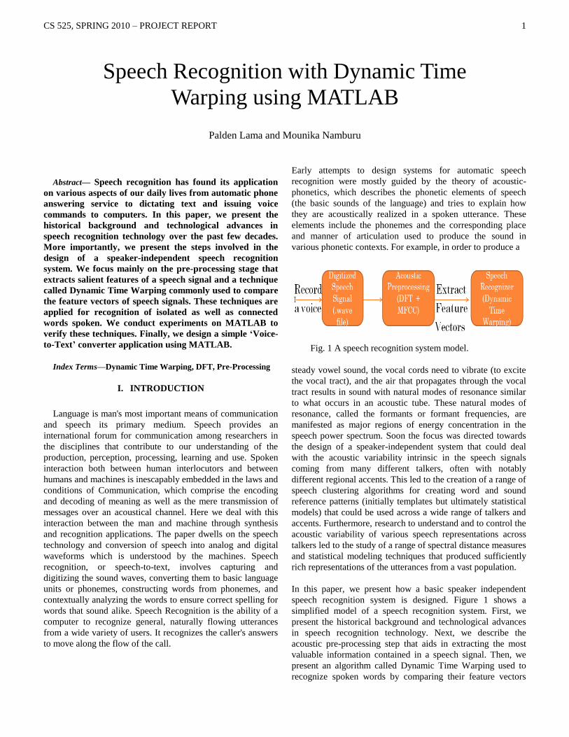
Fig. 1 A speech recognition system model.

steady vowel sound, the vocal cords need to vibrate (to excite

the vocal tract), and the air that propagates through the vocal

tract results in sound with natural modes of resonance similar

to what occurs in an acoustic tube. These natural modes of

resonance, called the formants or formant frequencies, are

manifested as major regions of energy concentration in the

speech power spectrum. Soon the focus was directed towards

the design of a speaker-independent system that could deal

with the acoustic variability intrinsic in the speech signals

coming from many different talkers, often with notably

different regional accents. This led to the creation of a range of

speech clustering algorithms for creating word and sound

reference patterns (initially templates but ultimately statistical

models) that could be used across a wide range of talkers and

accents. Furthermore, research to understand and to control the

acoustic variability of various speech representations across

talkers led to the study of a range of spectral distance measures

and statistical modeling techniques that produced sufficiently

rich representations of the utterances from a vast population.

In this paper, we present how a basic speaker independent

speech recognition system is designed. Figure 1 shows a

simplified model of a speech recognition system. First, we

present the historical background and technological advances

in speech recognition technology. Next, we describe the

acoustic pre-processing step that aids in extracting the most

valuable information contained in a speech signal. Then, we

present an algorithm called Dynamic Time Warping used to

recognize spoken words by comparing their feature vectors

Speech Recognition with Dynamic Time

Warping using MATLAB

Palden Lama and Mounika Namburu


2

with a database of representative feature vectors. We conduct

experiments in MATLAB to verify acoustic pre-processing

algorithms including DFT (Discrete Fourier Transform), MEL

ceptral transformation and pattern recognition algorithm

(Dynamic Time Warping). We also build a simple Voice-To-

Text converter application using MATLAB.

The structure of this paper is as follows. Section 2 reviews the

history of speech recognition technology and its applications.

Section 3 presents the acoustic pre-processing step commonly

used in any speech recognition system. Section 4 describes the

Dynamic Time Warping algorithm. Section 5 presents the

experimental results obtained using MATLAB. Section 6

concludes the paper.

II. HISTORY AND APPLICATIONS

The first speech recognizer appeared in 1952 and consisted

of a device for the recognition of single spoken digits. Another

early device was the IBM Shoebox, exhibited at the 1964 New

York World's Fair. Speech recognition technology has also

been a topic of great interest to a broad general population

since it became popularized in several blockbuster movies of

the 1960‟s and 1970‟s, most notably Stanley Kubrick‟s

acclaimed movie “2001: A Space Odyssey”. In this movie, an intelligent computer named “HAL” spoke in a natural

sounding voice and was able to recognize and understand

fluently spoken speech, and respond accordingly. This

anthropomorphism of HAL made the general public aware of

the potential of intelligent machines. In the famous Star Wars

saga, George Lucas extended the abilities of intelligent

machines by making them mobile as well as intelligent and the

droids like R2D2 and C3PO were able to speak naturally,

recognize and understand fluent speech, and move around and

interact with their environment, with other droids, and with the

human population at large. In 1988, in the technology

community, Apple Computer created a vision of speech

technology and computers for the year 2011, titled

“Knowledge Navigator”, which defined the concepts of a

Speech User Interface (SUI) and a Multimodal User Interface

(MUI) along with the theme of intelligent voice-enabled agents. This video had a dramatic effect in the technical

community and focused technology efforts, especially in the area of visual talking agents.

Throughout the course of development of such systems,

knowledge of speech production and perception was used in

establishing the technological foundation for the resulting

speech recognizers. Major advances, however, were brought

about in the 1960‟s and 1970‟s via the introduction of

advanced speech representations based on LPC analysis and

cepstral analysis methods, and in the 1980‟s through the

introduction of rigorous statistical methods based on hidden

Markov models. All of this came about because of significant

research contributions from academia, private industry and the

government. As the technology continues to mature, it is clear

that many new applications will emerge and become part of

our way of life – thereby taking full advantage of machines

that are partially able to mimic human speech capabilities.

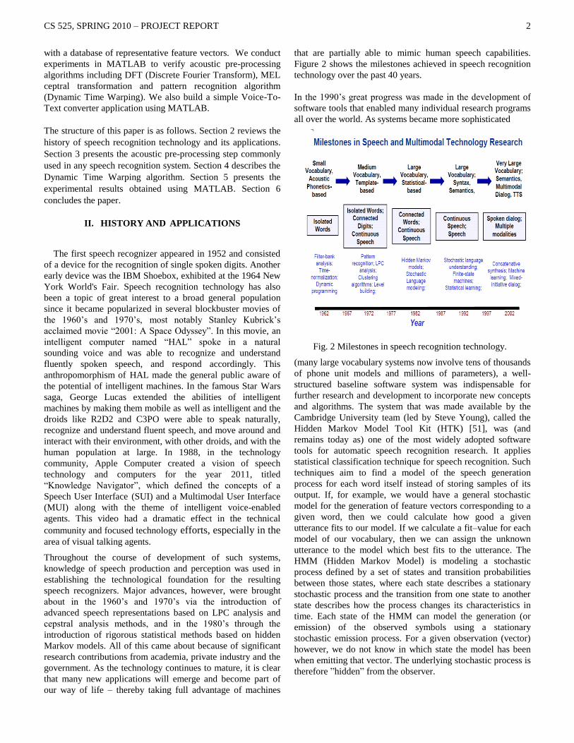
Figure 2 shows the milestones achieved in speech recognition

technology over the past 40 years.

In the 1990‟s great progress was made in the development of

software tools that enabled many individual research programs

all over the world. As systems became more sophisticated

Fig. 2 Milestones in speech recognition technology.

(many large vocabulary systems now involve tens of thousands

of phone unit models and millions of parameters), a well-

structured baseline software system was indispensable for

further research and development to incorporate new concepts

and algorithms. The system that was made available by the

Cambridge University team (led by Steve Young), called the

Hidden Markov Model Tool Kit (HTK) [51], was (and

remains today as) one of the most widely adopted software

tools for automatic speech recognition research. It applies

statistical classification technique for speech recognition. Such

techniques aim to find a model of the speech generation

process for each word itself instead of storing samples of its

output. If, for example, we would have a general stochastic

model for the generation of feature vectors corresponding to a

given word, then we could calculate how good a given

utterance fits to our model. If we calculate a fit–value for each

model of our vocabulary, then we can assign the unknown

utterance to the model which best fits to the utterance. The

HMM (Hidden Markov Model) is modeling a stochastic

process defined by a set of states and transition probabilities

between those states, where each state describes a stationary

stochastic process and the transition from one state to another

state describes how the process changes its characteristics in

time. Each state of the HMM can model the generation (or

emission) of the observed symbols using a stationary

stochastic emission process. For a given observation (vector)

however, we do not know in which state the model has been

when emitting that vector. The underlying stochastic process is

therefore ”hidden” from the observer.


3

Today, speech recognition applications include voice dialing

(e.g., "Call home"), call routing (e.g., "I would like to make a

collect call"), domestic appliance control, search (e.g., find a

podcast where particular words were spoken), simple data

entry (e.g., entering a credit card number), preparation of

structured documents (e.g., a radiology report), speech-to-text

processing (e.g., word processors or emails), and aircraft

(usually termed Direct Voice Input). One of the most notable

domains for the commercial application of speech recognition

in the United States has been health care and in particular the

work of the medical transcriptionist (MT). Other domains of

Speech Recognition applications are Military, Telephony,

People with disabilities, Telematics, Hands-free computing,

Home automation, etc. Speech recognition softwares such as

CMU Sphinx, Julius and Simon are freely available. Some

proprietary softwares available in market are AT&T

WATSON, HTK (copyrighted by Microsoft), Voice Finger

(for Windows Vista and Windows 7), Dragon

NaturallySpeaking from Nuance Communications (utilized

Hidden Markov Models), e-Speaking (for Windows XP) and

IBM ViaVoice.

III. ACOUSTIC PRE-PROCESSING

When producing speech sounds, the air flow from a speaker

lungs first passes the glottis and then throat and mouth.

Depending on which speech sound you articulate, the speech

signal can be excited in three possible ways:

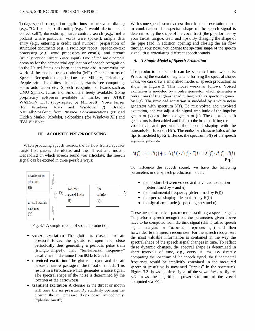
Fig. 3.1 A simple model of speech production.

voiced excitation The glottis is closed. The air

pressure forces the glottis to open and close

periodically thus generating a periodic pulse train

(triangle–shaped). This ”fundamental frequency”

usually lies in the range from 80Hz to 350Hz.

unvoiced excitation The glottis is open and the air

passes a narrow passage in the throat or mouth. This

results in a turbulence which generates a noise signal.

The spectral shape of the noise is determined by the

location of the narrowness.

transient excitation A closure in the throat or mouth

will raise the air pressure. By suddenly opening the

closure the air pressure drops down immediately.

(”plosive burst”)

With some speech sounds these three kinds of excitation occur

in combination. The spectral shape of the speech signal is

determined by the shape of the vocal tract (the pipe formed by

your throat, tongue, teeth and lips). By changing the shape of

the pipe (and in addition opening and closing the air flow

through your nose) you change the spectral shape of the speech

signal, thus articulating different speech sounds.

A. A Simple Model of Speech Production

The production of speech can be separated into two parts:

Producing the excitation signal and forming the spectral shape.

Thus, we can draw a simplified model of speech production as

shown in Figure 3. This model works as follows: Voiced

excitation is modeled by a pulse generator which generates a

pulse train (of triangle–shaped pulses) with its spectrum given

by P(f). The unvoiced excitation is modeled by a white noise

generator with spectrum N(f). To mix voiced and unvoiced

excitation, one can adjust the signal amplitude of the impulse

generator (v) and the noise generator (u). The output of both

generators is then added and fed into the box modeling the

vocal tract and performing the spectral shaping with the

transmission function H(f). The emission characteristics of the

lips is modeled by R(f). Hence, the spectrum S(f) of the speech

signal is given as:

To influence the speech sound, we have the following

parameters in our speech production model:

the mixture between voiced and unvoiced excitation

(determined by v and u)

the fundamental frequency (determined by P(f))

the spectral shaping (determined by H(f))

the signal amplitude (depending on v and u)

These are the technical parameters describing a speech signal.

To perform speech recognition, the parameters given above

have to be computed from the time signal (this is called speech

signal analysis or ”acoustic preprocessing”) and then

forwarded to the speech recognizer. For the speech recognizer,

the most valuable information is contained in the way the

spectral shape of the speech signal changes in time. To reflect

these dynamic changes, the spectral shape is determined in

short intervals of time, e.g., every 10 ms. By directly

computing the spectrum of the speech signal, the fundamental

frequency would be implicitly contained in the measured

spectrum (resulting in unwanted ”ripples” in the spectrum).

Figure 3.2 shows the time signal of the vowel /a:/ and figure.

3.3 shows the logarithmic power spectrum of the vowel

computed via FFT.

..Eq. 1


4

Fig. 3.2 Time signal of the vowel /a:/ (fs = 11kHz, length

= 100ms). The high peaks in the time signal are caused by the

pulse train P(f) generated by voiced excitation.

Fig. 3.3 Log power spectrum of the vowel /a:/ (fs =

11kHz, N = 512). The ripples in the spectrum are caused by

P(f).

B. Cepstral Transformation

As shown above, the direct computation of the power spectrum

from the speech signal results in a spectrum containing

”ripples” caused by the excitation spectrum X(f). Depending

on the implementation of the acoustic preprocessing however,

special transformations are used to separate the excitation

spectrum X(f) from the spectral shaping of the vocal tract H(f).

Thus, a smooth spectral shape (without the ripples), which

represents H(f) can be estimated from the speech signal. Most

speech recognition systems use the so–called mel frequency

cepstral coefficients (MFCC) and its first (and sometimes

second) derivative in time to better reflect dynamic changes.

Since the transmission function of the vocal tract H(f) is

multiplied with the spectrum of the excitation signal X(f), we

had those unwanted ”ripples” in the spectrum. For the speech

recognition task, a smoothed spectrum is required which

should represent H(f) but not X(f). To cope with this problem,

cepstral analysis is used. If we look at Equation 1, we can

separate the product of spectral functions into the interesting

vocal tract spectrum and the part describing the excitation and

emission properties:

We can now transform the product of the spectral functions to

a sum by taking the logarithm on both sides of the equation:

This holds also for the absolute values of the power spectrum

and also for their squares:

In figure 3.3 we see an example of the log power spectrum,

which contains unwanted ripples caused by the excitation

signal U(f) = X(f) · R(f). In the log–spectral domain we could

now subtract the unwanted portion of the signal, if we knew

|U(f)|2 exactly. But all we know is that U(f) produces the

”ripples”, which now are an additive component in the log–

spectral domain, and that if we would interpret this log–

spectrum as a time signal, the ”ripples” would have a ”high

frequency” compared to the spectral shape of |H(f)|. To get rid

of the influence of U(f), one would have to get rid of the

”high-frequency” parts of the log–spectrum (remember, we are

dealing with the spectral coefficients as if they would represent

a time signal). This would be a kind of low–pass filtering.

The filtering can be done by transforming the log–spectrum

back into the time–domain (in the following, FT −1

denotes the

inverse Fourier transform):

The inverse Fourier transform brings us back to the time–

domain (d is also called the delay or quefrency), giving the so–

called cepstrum (a reversed ”spectrum”). Figure 3.4 shows the

result of the inverse DFT applied on the log power spectrum

shown in fig. 3.3. The peak in the cepstrum reflects the ripples

of the log power spectrum. The low–pass filtering of our

energy spectrum can now be done by setting the higher-valued

coefficients of ceptrum to zero and then transforming back into

the frequency domain. The process of filtering in the cepstral

domain is also called liftering. In figure 3.4, all coefficients

left of the vertical line were set to zero and the resulting signal

was transformed back into the frequency domain, as shown in

fig. 3.5. One can clearly see that this results in a ”smoothed”

version of the log power spectrum if we compare figures 3.3

and 3.5.

Fig. 3.4 Cepstrum of the vowel /a:/ (fs = 11kHz, N = 512).

The ripples in the spectrum result in a peak in the cepstrum.


5

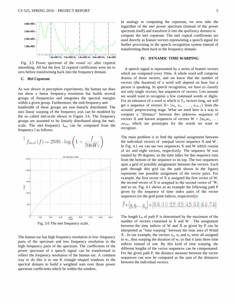
Fig. 3.5 Power spectrum of the vowel /a:/ after cepstral

smoothing. All but the first 32 cepstral coefficients were set to

zero before transforming back into the frequency domain.

C. Mel Cepstrum

As was shown in perception experiments, the human ear does

not show a linear frequency resolution but builds several

groups of frequencies and integrates the spectral energies

within a given group. Furthermore, the mid-frequency and

bandwidth of these groups are non–linearly distributed. The

non–linear warping of the frequency axis can be modeled by

the so–called mel-scale shown in Figure 3.6. The frequency

groups are assumed to be linearly distributed along the mel-

scale. The mel–frequency fmel can be computed from the

frequency f as follows:

Fig. 3.6 The mel frequency scale.

The human ear has high frequency resolution in low–frequency

parts of the spectrum and low frequency resolution in the

high–frequency parts of the spectrum. The coefficients of the

power spectrum of a speech signal can be transformed to

reflect the frequency resolution of the human ear. A common

way to do this is to use K triangle–shaped windows in the

spectral domain to build a weighted sum over those power

spectrum coefficients which lie within the window.

In analogy to computing the cepstrum, we now take the

logarithm of the mel power spectrum (instead of the power

spectrum itself) and transform it into the quefrency domain to

compute the mel cepstrum. The mel ceptral coefficients are

used directly as feature vectors representing a speech signal for

further processing in the speech recognition system instead of

transforming them back to the frequency domain.

IV. DYNAMIC TIME WARPING

A speech signal is represented by a series of feature vectors

which are computed every 10ms. A whole word will comprise

dozens of those vectors, and we know that the number of

vectors (the duration) of a word will depend on how fast a

person is speaking. In speech recognition, we have to classify

not only single vectors, but sequences of vectors. Lets assume

we would want to recognize a few command words or digits.

For an utterance of a word w which is TX vectors long, we will

get a sequence of vectors X= {x0, x1, . . . , xTX−1} from the

acoustic preprocessing stage. What we need here is a way to

compute a ”distance” between this unknown sequence of

vectors X and known sequences of vectors W = {w0,w1, . . .

,wTW} which are prototypes for the words we want to

recognize.

The main problem is to find the optimal assignment between

the individual vectors of unequal vector sequence X and W .

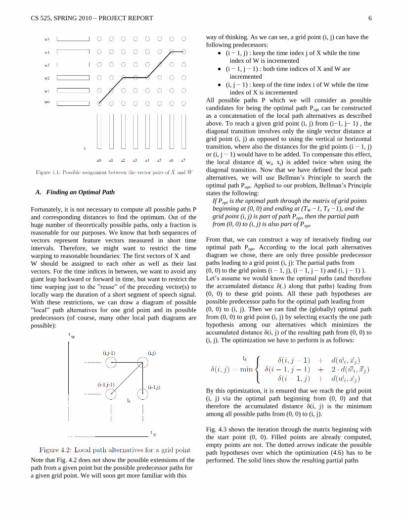
In Fig. 4.1 we can see two sequences X and W which consist

of six and eight vectors, respectively. The sequence W was

rotated by 90 degrees, so the time index for this sequence runs

from the bottom of the sequence to its top. The two sequences

span a grid of possible assignments between the vectors. Each

path through this grid (as the path shown in the figure)

represents one possible assignment of the vector pairs. For

example, the first vector of X is assigned the first vector of W,

the second vector of X is assigned to the second vector of ˜W,

and so on. Fig. 4.1 shows as an example the following path P

given by the sequence of time index pairs of the vector

sequences (or the grid point indices, respectively):

The length LP of path P is determined by the maximum of the

number of vectors contained in X and W . The assignment

between the time indices of W and X as given by P can be

interpreted as ”time warping” between the time axes of Wand

X . In our example, the vectors x2, x3 and x4 were all assigned

to w2, thus warping the duration of w2 so that it lasts three time

indices instead of one. By this kind of time warping, the

different lengths of the vector sequences can be compensated.

For the given path P, the distance measure between the vector

sequences can now be computed as the sum of the distances

between the individual vectors.


6

A. Finding an Optimal Path

Fortunately, it is not necessary to compute all possible paths P

and corresponding distances to find the optimum. Out of the

huge number of theoretically possible paths, only a fraction is

reasonable for our purposes. We know that both sequences of

vectors represent feature vectors measured in short time

intervals. Therefore, we might want to restrict the time

warping to reasonable boundaries: The first vectors of X and

W should be assigned to each other as well as their last

vectors. For the time indices in between, we want to avoid any

giant leap backward or forward in time, but want to restrict the

time warping just to the ”reuse” of the preceding vector(s) to

locally warp the duration of a short segment of speech signal.

With these restrictions, we can draw a diagram of possible

”local” path alternatives for one grid point and its possible

predecessors (of course, many other local path diagrams are

possible):

Note that Fig. 4.2 does not show the possible extensions of the

path from a given point but the possible predecessor paths for

a given grid point. We will soon get more familiar with this

way of thinking. As we can see, a grid point (i, j) can have the

following predecessors:

(i − 1, j) : keep the time index j of X while the time

index of W is incremented

(i − 1, j − 1) : both time indices of X and W are

incremented

(i, j − 1) : keep of the time index i of W while the time

index of X is incremented

All possible paths P which we will consider as possible

candidates for being the optimal path Popt can be constructed

as a concatenation of the local path alternatives as described

above. To reach a given grid point (i, j) from (i−1, j− 1) , the

diagonal transition involves only the single vector distance at

grid point (i, j) as opposed to using the vertical or horizontal

transition, where also the distances for the grid points (i − 1, j)

or (i, j − 1) would have to be added. To compensate this effect,

the local distance d( wi, xj) is added twice when using the

diagonal transition. Now that we have defined the local path

alternatives, we will use Bellman‟s Principle to search the

optimal path Popt. Applied to our problem, Bellman‟s Principle

states the following:

If Popt is the optimal path through the matrix of grid points

beginning at (0, 0) and ending at (TW −1, TX −1), and the

grid point (i, j) is part of path Popt, then the partial path

from (0, 0) to (i, j) is also part of Popt.

From that, we can construct a way of iteratively finding our

optimal path Popt. According to the local path alternatives

diagram we chose, there are only three possible predecessor

paths leading to a grid point (i, j): The partial paths from

(0, 0) to the grid points (i − 1, j), (i − 1, j − 1) and (i, j − 1) ).

Let‟s assume we would know the optimal paths (and therefore

the accumulated distance δ(.) along that paths) leading from

(0, 0) to these grid points. All these path hypotheses are

possible predecessor paths for the optimal path leading from

(0, 0) to (i, j). Then we can find the (globally) optimal path

from (0, 0) to grid point (i, j) by selecting exactly the one path

hypothesis among our alternatives which minimizes the

accumulated distance δ(i, j) of the resulting path from (0, 0) to

(i, j). The optimization we have to perform is as follows:

By this optimization, it is ensured that we reach the grid point

(i, j) via the optimal path beginning from (0, 0) and that

therefore the accumulated distance δ(i, j) is the minimum

among all possible paths from (0, 0) to (i, j).

Fig. 4.3 shows the iteration through the matrix beginning with

the start point (0, 0). Filled points are already computed,

empty points are not. The dotted arrows indicate the possible

path hypotheses over which the optimization (4.6) has to be

performed. The solid lines show the resulting partial paths


7

after the decision for one of the path hypotheses during the

optimization step. Once we reached the top–right corner of our

matrix, the accumulated distance δ(TW − 1, TX −1) is the

distance D( W , X ) between the vector sequences. The

optimal path is known only after the termination of the

algorithm, when we have made the last recombination for the

three possible path hypotheses leading to the top–right grid

point (TW −1, TX −1). Once this decision is made, the optimal

path can be found by reversely following all the local decisions

down to the origin (0, 0). This procedure is called

backtracking.

B. Recognition of Isolated Words

While the description of the DTW classification algorithm

might let us think that one would compute all the distances

sequentially and then select the minimum distance, it is more

useful in practical applications to compute all the distances

between the unknown vector sequence and the class prototypes

in parallel. This is possible since the DTW algorithm needs

only the values for time index t and (t−1) and therefore there is

no need to wait until the utterance of the unknown vector

sequence is completed. Instead, one can start with the

recognition process immediately as soon as the utterance

begins (we will not deal with the question of how to recognize

the start and end of an utterance here). To do so, we have to

reorganize our search space a little bit. First, lets assume

the total number of all prototypes over all classes is given by

M. If we want to compute the distances to all M prototypes

simultaneously, we have to keep track of the accumulated

distances between the unknown vector sequence and the

prototype sequences individually. Hence, instead of the

column (or two columns, depending on the implementation)

Fig. 4.4 Classification task redefined as finding the optimal

path among all prototype words

we used to hold the accumulated distance values for all grid

points, we now have to provide M columns during the DTW

procedure. Now we introduce an additional ”virtual” grid point

together with a specialized local path alternative for this point:

The possible predecessors for this point are defined to be the

upper–right grid points of the individual grid matrices of the

prototypes. In other words, the virtual grid point can only be

reached from the end of each prototype word, and among all

the possible prototype words, the one with the smallest

accumulated distance is chosen. By introducing this virtual

grid point, the classification task itself (selecting the class with

the smallest class distance) is integrated into the framework of

finding the optimal path. Now all we have to do is to run the

DTW algorithm for each time index j and along all columns of

all prototype sequences. At the last time slot (TW − 1) we

perform the optimization step for the virtual grid point, i.e, the

predecessor grid point to the virtual grid point is chosen to be

the prototype word having the smallest accumulated distance.

Note that the search space we have to consider is spanned by

the length of the unknown vector sequence on one hand and

the sum of the length of all prototype sequences of all classes

on the other hand. Figure 4.4 shows the individual grids for the

prototypes (only three are shown here) and the selected

optimal path to the virtual grid point. The backtracking

procedure can of course be restricted to keeping track of the

final optimization step when the best predecessor for the

virtual grid point is chosen. The classification task is then

performed by assigning the unknown vector sequence to the


8

very class to which the prototype belongs whose word end grid

point was chosen.

C. Recognition of Connected Words

When we need to recognize a sequence of words (like a credit

card number or telephone number) the classification task can

be divided into two different subtasks: The segmentation of the

utterance, i.e., finding the boundaries between the words and

the classification of the individual words within their

boundaries. As one can imagine, the number of possible

combinations of words of a given vocabulary together with the

fact that each word may widely vary in its length provides for a

huge number of combinations to be considered during the

classification. Fortunately, there is a solution for the problem,

which is able to find the word boundaries and to classify the

words within the boundaries in one single step. If we want to

apply the DP algorithm to our new task, we will first have to

define the search space for our new task. For simplicity, let‟s

assume that each word of our vocabulary is represented by

only one prototype, which will make the notation a bit easier

for us. An unknown utterance of a given length TX will contain

several words out of our vocabulary, but we do not know

which words these are and at what time index they begin or

end. Therefore, we will have to match the utterance against all

prototypes and we will have to test for all possible word ends

and word beginnings. The optimal path we want to find with

our DP algorithm must therefore be allowed to run through a

search space which is spanned by the set of all vectors of all

prototypes in one dimension and by the vector sequence of the

unknown utterance in the other dimension, as is shown in Fig.

4.5.

Fig 4.5 DTW Algorithm for Connected Word

Recognition

Now we have to modify our definition of local path

alternatives for the first vector of each prototype: The first

vector of a prototype denotes the beginning of the word. In the

case of isolated word recognition, the grid point corresponding

to that vector was initialized in the first column with the

distance between the first vector of the prototype and the first

vector of the utterance. During the DP, i.e., while we were

moving from column to column, this grid point had only one

predecessor, it could only be preceded by the same grid point

in the preceding column (the ”horizontal” transition),

indicating that the first vector of the prototype sequence was

warped in time to match the next vector of the unknown

utterance. For connected word recognition however, the grid

point corresponding to the first vector of a prototype has more

path alternatives: It may either select the same grid point in the

preceding column (this is the ”horizontal” transition, which we

already know), or it may select every last grid point (word end,

is) of all prototypes (including the prototype itself ) of the

preceding column as a possible predecessor for between–word

path recombination. In this case, the prototype word under

consideration is assumed to start at the current time index and

the word whose word end was chosen is assumed to end at the

time index before. Fig. 4.6 shows the local path alternatives for

the first grid point of the column associated with a prototype.

By allowing these additional path alternatives, we allow the

optimal path to run through several words in our search space,

where a word boundary can be found at those times at which

the path jumps from the last grid point of a prototype column

to the first grid point of a prototype column.

Fig. 4.6 Local path alternatives of the first grid point of a

column


9

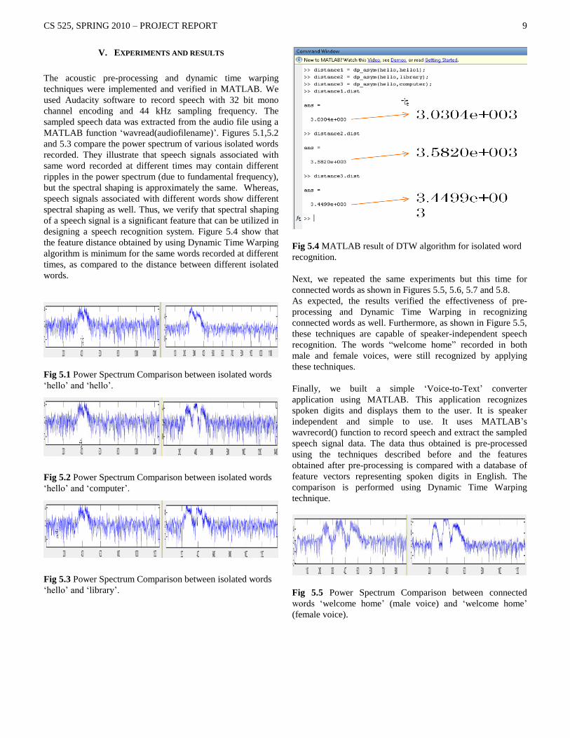
V. EXPERIMENTS AND RESULTS

The acoustic pre-processing and dynamic time warping

techniques were implemented and verified in MATLAB. We

used Audacity software to record speech with 32 bit mono

channel encoding and 44 kHz sampling frequency. The

sampled speech data was extracted from the audio file using a

MATLAB function „wavread(audiofilename)‟. Figures 5.1,5.2

and 5.3 compare the power spectrum of various isolated words

recorded. They illustrate that speech signals associated with

same word recorded at different times may contain different

ripples in the power spectrum (due to fundamental frequency),

but the spectral shaping is approximately the same. Whereas,

speech signals associated with different words show different

spectral shaping as well. Thus, we verify that spectral shaping

of a speech signal is a significant feature that can be utilized in

designing a speech recognition system. Figure 5.4 show that

the feature distance obtained by using Dynamic Time Warping

algorithm is minimum for the same words recorded at different

times, as compared to the distance between different isolated

words.

Fig 5.1 Power Spectrum Comparison between isolated words

„hello‟ and „hello‟.


„hello‟ and „computer‟.


„hello‟ and „library‟.

Fig 5.4 MATLAB result of DTW algorithm for isolated word

recognition.

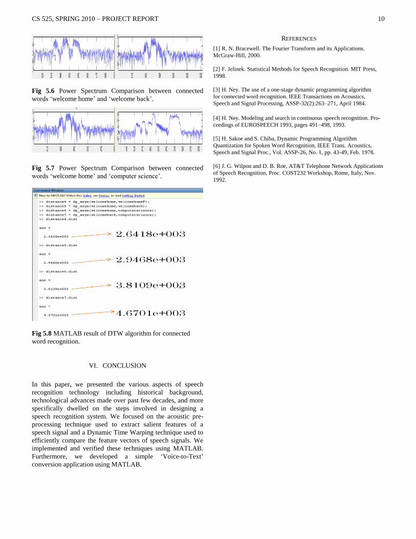
Next, we repeated the same experiments but this time for

connected words as shown in Figures 5.5, 5.6, 5.7 and 5.8.

As expected, the results verified the effectiveness of pre-

processing and Dynamic Time Warping in recognizing

connected words as well. Furthermore, as shown in Figure 5.5,

these techniques are capable of speaker-independent speech

recognition. The words “welcome home” recorded in both

male and female voices, were still recognized by applying

these techniques.

Finally, we built a simple „Voice-to-Text‟ converter

application using MATLAB. This application recognizes

spoken digits and displays them to the user. It is speaker

independent and simple to use. It uses MATLAB‟s

wavrecord() function to record speech and extract the sampled

speech signal data. The data thus obtained is pre-processed

using the techniques described before and the features

obtained after pre-processing is compared with a database of

feature vectors representing spoken digits in English. The

comparison is performed using Dynamic Time Warping

technique.

Fig 5.5 Power Spectrum Comparison between connected

words „welcome home‟ (male voice) and „welcome home‟

(female voice).


10


words „welcome home‟ and „welcome back‟.


words „welcome home‟ and „computer science‟.

Fig 5.8 MATLAB result of DTW algorithm for connected

word recognition.

VI. CONCLUSION

In this paper, we presented the various aspects of speech

recognition technology including historical background,

technological advances made over past few decades, and more

specifically dwelled on the steps involved in designing a

speech recognition system. We focused on the acoustic pre-

processing technique used to extract salient features of a

speech signal and a Dynamic Time Warping technique used to

efficiently compare the feature vectors of speech signals. We

implemented and verified these techniques using MATLAB.

Furthermore, we developed a simple „Voice-to-Text‟

conversion application using MATLAB.

REFERENCES

[1] R. N. Bracewell. The Fourier Transform and its Applications.

McGraw-Hill, 2000.

[2] F. Jelinek. Statistical Methods for Speech Recognition. MIT Press,

1998.

[3] H. Ney. The use of a one-stage dynamic programming algorithm

for connected word recognition. IEEE Transactions on Acoustics,

Speech and Signal Processing, ASSP-32(2):263–271, April 1984.

[4] H. Ney. Modeling and search in continuous speech recognition. Pro-

ceedings of EUROSPEECH 1993, pages 491–498, 1993.

[5] H. Sakoe and S. Chiba, Dynamic Programming Algorithm

Quantization for Spoken Word Recognition, IEEE Trans. Acoustics,

Speech and Signal Proc., Vol. ASSP-26, No. 1, pp. 43-49, Feb. 1978.

[6] J. G. Wilpon and D. B. Roe, AT&T Telephone Network Applications

of Speech Recognition, Proc. COST232 Workshop, Rome, Italy, Nov.

1992.

speech recognition with dynamic time warping using matlab · cs 525, spring 2010 – project report...

Documents