speed emission/energy curves for ultra-low emission vehicles · 2019-08-08 · a set of...
TRANSCRIPT

[Keywords]
Speed emission/energy curves for ultra-low emission vehicles Final Report ___________________________________________________
Report for Department for Transport
RM3295 - SB 1523
ED 59731 –Final Report FR_Issue Number 2 | Date 23/06/2015 Ricardo-AEA in Confidence
Speed emission/energy curves for ultra-low emission vehicles | i
Ricardo-AEA in Confidence Ref: Ricardo-AEA/ED59731/FR_Issue Number 2
RICARDO-AEA
Customer: Contact: Department for Transport John Norris
Ricardo-AEA Ltd Gemini Building, Harwell, Didcot, OX11 0QR, United Kingdom t: +44 (0) 1235 75 3685 e: [email protected] Ricardo-AEA is certificated to ISO9001 and ISO14001
Customer reference:
RM3295 - SB 1523
Confidentiality, copyright & reproduction:
This report is the Copyright of Department of Transport/Ricardo-AEA Ltd and has been prepared by Ricardo-AEA Ltd under contract to Department for Transport dated 03/06/2014. The contents of this report may not be reproduced in whole or in part, nor passed to any organisation or person without the specific prior written permission of Department for Transport / Commercial manager, Ricardo-AEA Ltd. Ricardo-AEA Ltd accepts no liability whatsoever to any third party for any loss or damage arising from any interpretation or use of the information contained in this report, or reliance on any views expressed therein.
Author:
Guy Hitchcock, John Norris, Rebecca Rose, Tim Murrells, Edina Löhr, James Tate (Leeds U ITS)
Approved By:
Tim Murrells
Date:
23 June 2015
Ricardo-AEA reference:
Ref: ED59731- FR_Issue Number 2

Speed emission/energy curves for ultra-low emission vehicles | ii
Ricardo-AEA in Confidence Ref: Ricardo-AEA/ED59731/FR_Issue Number 2
RICARDO-AEA
Executive summary This project has developed a set of speed-energy/emission curves for a range of low emission vehicle technologies for use with the National Transport Model (NTM) and Webtag. The inclusion of these new technologies is to support the assessment of policies that will promote the uptake of such technologies in the future. The technologies covered in this project were:
Hybrid Electric Vehicles (HEVs) – both petrol and diesel and for cars and vans Battery Electric Vehicles (BEVs) – for both cars and vans Plugin Hybrid Electric Vehicles (PHEVs) – again petrol and diesel for both cars and vans Fuel cell electric vehicles (FCEVs) – for cars and vans Dedicated methane trucks – spark ignition (SI) vehicles in both rigid and articulated form Dual fuel methane trucks – compression ignition vehicles (CI) running on both methane and
diesel, for both rigid and articulated trucks. Small battery electric trucks – covering 3.5-7.5t and 7.5-12t rigid trucks.
Speed – energy/fuel consumption curves were developed for all vehicle types and NOx and PM curves were developed for the petrol, diesel and methane fuelled vehicles.
The curves have been generated from a range of data from existing literature, raw emissions/energy data and simulations. However, since many of the technologies are new or not even in production detailed real-world data were not easily available. For the light duty vehicles good speed dependant data were available either from raw data or simulations for petrol hybrid cars, diesel hybrid cars and battery electric cars. These data could be used for the direct derivation of the speed-energy/emission curves. For the other technologies the curves were either extrapolated from these core vehicle types or estimated from literature data.
With the heavy duty vehicle technologies the data are generally more limited. There was some speed dependant data available for dedicated and dual fuel methane trucks, which was complemented by literature data to derive the speed-energy/emission curves. The battery electric trucks were extrapolated from the curves developed for the larger class 3 vans and some larger electric truck data.
The robustness of the curves developed is limited by the available data and have more uncertainty than those for conventional petrol and diesel vehicles. However, they have been developed from relative changes in comparison with conventional vehicles and so are suitable for assessing relative changes in emission when looking at different levels of penetration of these vehicle technologies into the vehicle fleet.
In developing these curves several key points arose that should be noted and/or for further consideration:
Diesel hybrid cars/vans – it was clear from the analysis that these do not perform as well as petrol hybrids. There is some fuel consumption benefit but there is a clear NOx dis-benefit therefore their widespread adoption could be detrimental to air quality especially in urban areas.
Plugin hybrids – the performance of these is very strongly related to charging behaviour by users which has been represented by the concept of a ‘utility factor’. However, further work on this behavioural aspect is recommended to really understand how these vehicles will be used and hence the benefits they could bring. There is also the need for further information on emissions from different power train architectures between HEVs which can be charged from the mains and range-extended EVs.
Methane slip and greenhouse gas emissions – this project has only estimated CO2 emissions not wider GHG emissions. Methane slip from methane vehicles could have a significant impact on this and so the results from the ongoing methane slip project should be incorporated into any future updated of these curves.
Wider emission categories – consideration should be given to generating data on a wide set of emissions especially direct NO2 and non-exhaust particulates.
Speed emission/energy curves for ultra-low emission vehicles | iii
Ricardo-AEA in Confidence Ref: Ricardo-AEA/ED59731/FR_Issue Number 2
RICARDO-AEA
A set of speed-emission curves can be developed for each main low emission vehicle (ULEV) category in a spreadsheet provided with this report which when combined with year-specific fleet compositional data yield a fleet-average emission or energy consumption factor for each ULEV type in 5 year intervals from 2015-2040 tailored for use in the NTM. A qualitative uncertainty ranking has been considered in the emission curves developed for each main ULEV category. The relative differences in emission factors between different ULEV types and relative to conventional petrol and diesel equivalent vehicles can probably be assigned lower uncertainty than their absolute values.
Finally we recommend revisiting all the emission curves developed in this project as technology matures, more vehicles enter service, more data become available and new alternative concepts are developed.

Speed emission/energy curves for ultra-low emission vehicles | iv
Ricardo-AEA in Confidence Ref: Ricardo-AEA/ED59731/FR_Issue Number 2
RICARDO-AEA
Table of contents 1 Introduction ................................................................................................................ 1
2 Data sources and outline methodology ................................................................... 2 2.1 Overview of the core data sources .................................................................................... 2 2.2 Outline methodology for car and van curves ................................................................... 11 2.3 Outline methodology for HGV curves .............................................................................. 13 2.4 Summary data and method tables .................................................................................. 14
3 Emission curves for cars and vans ........................................................................ 18 3.1 Petrol Car HEVs .............................................................................................................. 18 3.2 Diesel HEV cars .............................................................................................................. 22 3.3 Battery electric vehicles (BEVs) ...................................................................................... 26 3.4 Plug-in HEV cars ............................................................................................................. 28 3.5 Fuel cell cars ................................................................................................................... 30 3.6 HEV vans ......................................................................................................................... 31 3.7 BEV, PHEV and fuel cell vans ......................................................................................... 35
4 Emission curves for HGVs ...................................................................................... 37 4.1 Dedicated methane fuelled vehicles ............................................................................... 37 4.2 Dual fuel vehicles ............................................................................................................ 41 4.3 Small electric trucks ........................................................................................................ 42
5 Aggregation tools .................................................................................................... 45 5.1 ULEV categories.............................................................................................................. 45 5.2 Weighting factors by main ULEV class ........................................................................... 47 5.3 Generation of EF curves ................................................................................................. 48 5.4 Further weighting and adjustment for HGV curves ......................................................... 49 5.5 Use of the Emission curves ............................................................................................. 49
6 Uncertainly assessment of ULEV emission curves ............................................... 51 6.1 Overview of main sources of uncertainties ..................................................................... 51 6.2 Uncertainties in emission curves for each ULEV category ............................................. 51 6.3 Completeness of the emission curves ............................................................................ 55 6.4 QA/QC considerations ..................................................................................................... 55
7 Conclusions ............................................................................................................. 57 Acknowledgements Glossary References

Speed emission/energy curves for ultra-low emission vehicles | 1
Ricardo-AEA in Confidence Ref: Ricardo-AEA/ED59731/FR_Issue Number 2
RICARDO-AEA
1 Introduction The objective of this project was to develop fuel/energy consumption and emission speed curves for a range of Low Emission Vehicles (LEVs) for use with the National Transport Model (NTM) and WebTAG. These fuel consumption and emission curves should be consistent with the existing curves currently used for conventional vehicles by the NTM and WebTAG. The purpose of developing these energy/emission curves for LEVs is to allow for modelling the impact of the future uptake of these technologies in response to policy measures.
The vehicles and technologies which are covered by the project are shown in Table 1. For each vehicle/technology type curves have been developed for fuel or energy use, CO2, NOx and PM10.
Table 1 Low Emission Vehicles for which speed emission/energy curves have been developed
Vehicle Type Fuel/Technology Type
Cars Petrol Hybrid Electric Vehicle (Petrol HEV) Diesel Hybrid Electric Vehicle (Diesel HEV) Petrol Plug-in Hybrid Electric Vehicle (Petrol PHEV) Diesel Plug-in Hybrid Electric Vehicle (Diesel PHEV) Battery Electric Vehicle (BEV) Fuel Cell Electric Vehicle (FCEV)
Light Goods Vehicles Petrol Hybrid Electric Vehicle Diesel Hybrid Electric Vehicle Petrol Plug-in Hybrid Electric Vehicle Diesel Plug-in Hybrid Electric Vehicle Battery Electric Vehicle Fuel Cell Electric Vehicle
Rigid Heavy Goods Vehicles Biomethane/ Natural Gas Vehicle Dual Fuel Diesel & Biomethane/ Natural Gas Vehicle Battery Electric Vehicle (3.5t -12t GVW only)
Articulated Heavy Goods vehicles Biomethane/ Natural Gas Vehicle Dual Fuel Diesel & Biomethane/ Natural Gas Vehicle
The development of these speed energy/emission curves was carried out through the following tasks:
Task 1 - review existing data on LEV energy use and emissions and identify gaps Task 2 – generation of additional LEV data through simulation or extrapolation models to fill
these gaps where appropriate Task 3 – use the existing and simulated data to derive the energy use and emission curves for
use in NTM and WebTag Task 4 - provide an uncertainty assessment for the derived factors
This is the final project report and provides the full results of the study. Section 2 provides an overview of the data and methodology used for the study. Section 3 sets out the results for cars and vans and section 4 sets out the results for the heavy goods vehicles. In section 5 we provide an overview of the tools developed for the aggregation of the emission function for use in the NTM and the final section 6 provides a discussion regarding the uncertainty and robustness of the results.
Accompanying this report are spreadsheets with the final emission curves functions and aggregation tools.
Speed emission/energy curves for ultra-low emission vehicles | 2
Ricardo-AEA in Confidence Ref: Ricardo-AEA/ED59731/FR_Issue Number 2
RICARDO-AEA
2 Data sources and outline methodology 2.1 Overview of the core data sources A number of data sources have been used to assess, derive and validate the emissions curves for this study. The key data sources cover:
Existing emissions models Manufacturers’ homologation data Literature results on real world emissions Simulation data using the PHEM model PEMS data from vehicle tests in the UK
2.1.1 Existing emission models In Europe the key transport emissions models and data are generated by organisations within the ERMES (European Research on Mobile Emissions) group1. ERMES aims to coordinate research (and measurement programmes) for the improvement of transport emission inventories in Europe and provides a clearinghouse for data and modelling tools. Its aim is to provide harmonised data for all EU transport emission models including COPERT2. COPERT is the source of emission factors recommended in the EMEP/EEA Emissions Inventory Guidebook, aimed at providing a common source of emission factors for national emission inventories across Europe and is the source of many of the factors used in the UK’s National Atmospheric Emissions Inventory (NAEI)3. The key models from the ERMES group are:
COPERT 4 (v10/11) Swiss-German-Austrian Handbook of Emission Factors (HBEFA 3.1) TNO’s VERSIT+ model Passenger and Heavy duty Emissions Model (PHEM)
In addition the project reviewed the US EPA MOVE model. At present there is very little data in any of these models in relation to the ultralow emission vehicles and so there is a clear gap in these models for these vehicle types. The exception is petrol hybrid cars with emissions data in COPERT, VERSIT, US MOVE model and PHEM. However, even this data is limited to a Euro 4 hybrid car in COPERT and a Euro 5 vehicle for simulation in PHEM.
Within all of these models there is the intention to develop such data in future releases.
2.1.2 Manufacturers’ data There are a growing number ultra-low emission vehicles being marketed in the UK especially in the car market in terms of hybrid electric vehicles (HEV’s), plug-in hybrid electric vehicles (PHEVs) and electric vehicles (EVs). Table 2 shows the number of vehicle models currently registered among the different low emission vehicle categories. For the passenger cars, a high number of petrol HEVs and EVs are available. A reasonable number of petrol PHEV and diesel HEV models were identified; however, diesel PHEVs are clearly underrepresented. For vans the picture is very one-sided. Except for one company producing diesel HEVs, all available low emission vans are EVs.
For the vehicles identified, manufacturers’ reported emission and consumption data were collected. Manufacturers only provide the data that is required for vehicle type approval. Using the Vehicle Certification Agency (VCA) vehicle registration database and crosschecking it with data provided on the manufacturers’ websites, average fuel consumption values for the regulatory urban, extra-urban and combined test cycle were obtained. Furthermore, emission values for a weighted average over urban and extra-urban laboratory test-cycles were collected.
1 http://www.ermes-group.eu/web/ 2 http://emisia.com/copert 3 http://naei.defra.gov.uk/
Speed emission/energy curves for ultra-low emission vehicles | 3
Ricardo-AEA in Confidence Ref: Ricardo-AEA/ED59731/FR_Issue Number 2
RICARDO-AEA
Table 2: Vehicles categorized by fuel type and technology
Passenger cars Petrol HEV 22 models Diesel HEV 6 models EVs 12 models Petrol PHEV 6 models Diesel PHEV 1 model
Vans Petrol HEV none Diesel HEV few EVs 13 models Petrol PHEV none Diesel PHEV none
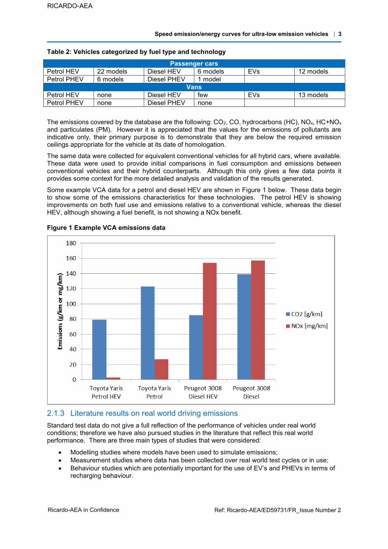
The emissions covered by the database are the following: CO2, CO, hydrocarbons (HC), NOx, HC+NOx and particulates (PM). However it is appreciated that the values for the emissions of pollutants are indicative only, their primary purpose is to demonstrate that they are below the required emission ceilings appropriate for the vehicle at its date of homologation.
The same data were collected for equivalent conventional vehicles for all hybrid cars, where available. These data were used to provide initial comparisons in fuel consumption and emissions between conventional vehicles and their hybrid counterparts. Although this only gives a few data points it provides some context for the more detailed analysis and validation of the results generated.
Some example VCA data for a petrol and diesel HEV are shown in Figure 1 below. These data begin to show some of the emissions characteristics for these technologies. The petrol HEV is showing improvements on both fuel use and emissions relative to a conventional vehicle, whereas the diesel HEV, although showing a fuel benefit, is not showing a NOx benefit.
Figure 1 Example VCA emissions data
2.1.3 Literature results on real world driving emissions Standard test data do not give a full reflection of the performance of vehicles under real world conditions; therefore we have also pursued studies in the literature that reflect this real world performance. There are three main types of studies that were considered:
Modelling studies where models have been used to simulate emissions; Measurement studies where data has been collected over real world test cycles or in use; Behaviour studies which are potentially important for the use of EV’s and PHEVs in terms of
recharging behaviour.
Speed emission/energy curves for ultra-low emission vehicles | 4
Ricardo-AEA in Confidence Ref: Ricardo-AEA/ED59731/FR_Issue Number 2
RICARDO-AEA
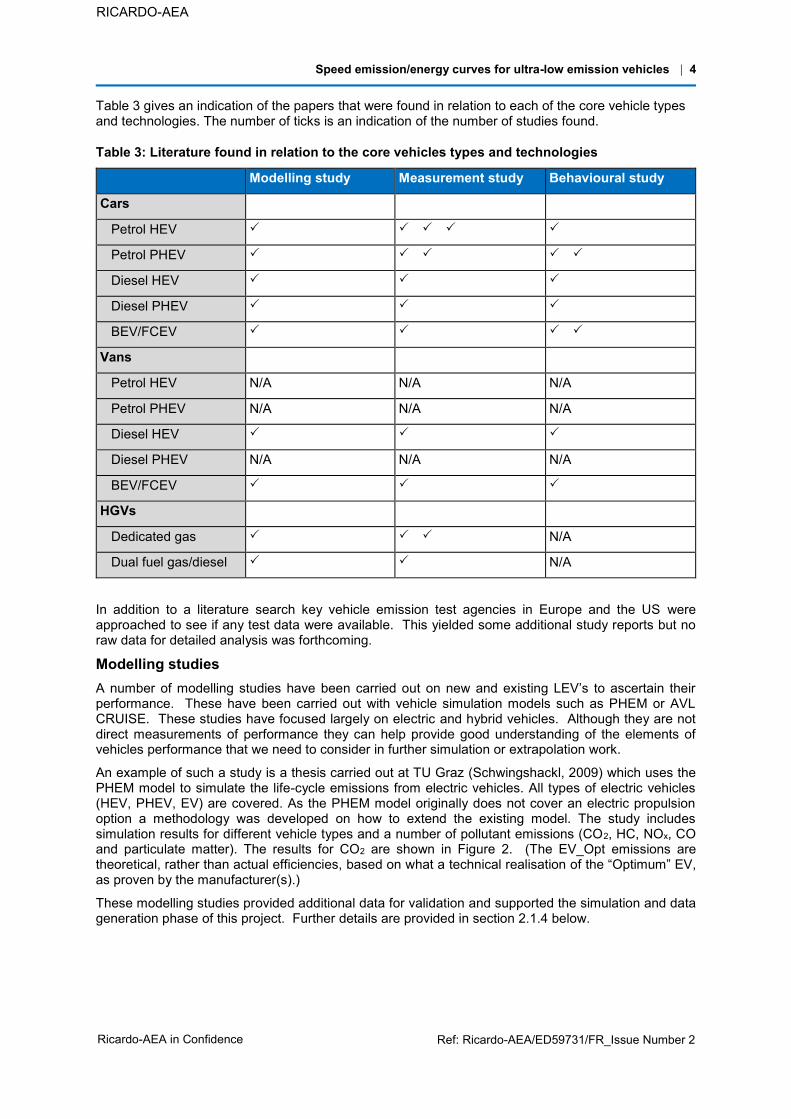
Table 3 gives an indication of the papers that were found in relation to each of the core vehicle types and technologies. The number of ticks is an indication of the number of studies found.
Table 3: Literature found in relation to the core vehicles types and technologies
Modelling study Measurement study Behavioural study
Cars
Petrol HEV
Petrol PHEV
Diesel HEV
Diesel PHEV
BEV/FCEV
Vans
Petrol HEV N/A N/A N/A
Petrol PHEV N/A N/A N/A
Diesel HEV
Diesel PHEV N/A N/A N/A
BEV/FCEV
HGVs
Dedicated gas N/A
Dual fuel gas/diesel N/A
In addition to a literature search key vehicle emission test agencies in Europe and the US were approached to see if any test data were available. This yielded some additional study reports but no raw data for detailed analysis was forthcoming.
Modelling studies A number of modelling studies have been carried out on new and existing LEV’s to ascertain their performance. These have been carried out with vehicle simulation models such as PHEM or AVL CRUISE. These studies have focused largely on electric and hybrid vehicles. Although they are not direct measurements of performance they can help provide good understanding of the elements of vehicles performance that we need to consider in further simulation or extrapolation work.
An example of such a study is a thesis carried out at TU Graz (Schwingshackl, 2009) which uses the PHEM model to simulate the life-cycle emissions from electric vehicles. All types of electric vehicles (HEV, PHEV, EV) are covered. As the PHEM model originally does not cover an electric propulsion option a methodology was developed on how to extend the existing model. The study includes simulation results for different vehicle types and a number of pollutant emissions (CO2, HC, NOx, CO and particulate matter). The results for CO2 are shown in Figure 2. (The EV_Opt emissions are theoretical, rather than actual efficiencies, based on what a technical realisation of the “Optimum” EV, as proven by the manufacturer(s).)
These modelling studies provided additional data for validation and supported the simulation and data generation phase of this project. Further details are provided in section 2.1.4 below.

Speed emission/energy curves for ultra-low emission vehicles | 5
Ricardo-AEA in Confidence Ref: Ricardo-AEA/ED59731/FR_Issue Number 2
RICARDO-AEA
Figure 2: PHEM simulation results - CO2 emissions for different vehicle types4
Measurement studies There are three types of measurement studies that have been carried out:
Laboratory tests using a chassis dynamometer and real world drive cycles, which is the traditional testing approach
Remote sensing data that uses a static beam projected across a road to analyse tailpipe emissions from passing vehicles
Portable Emissions Monitoring Systems (PEMS) where emissions tests are carried out on vehicles in real traffic situations
Laboratory tests
Most of the measurement data are collected in laboratories using chassis dynamometer tests. An example of this kind of data is the Advanced Vehicle Testing Activity (AVTA) of the Idaho National Laboratory (INL) in the US which provides benchmark data for technology modelling and research and development programs. A number of advanced technologies for light-, medium-, and heavy duty vehicles are covered, including Hybrids, Plug-in Hybrids and Electric Vehicles. Vehicle test procedures that accurately measure real-world vehicle emission performance are developed and then used to test advanced technologies in production and pre-production (Idaho National Laboratory, 2014a).
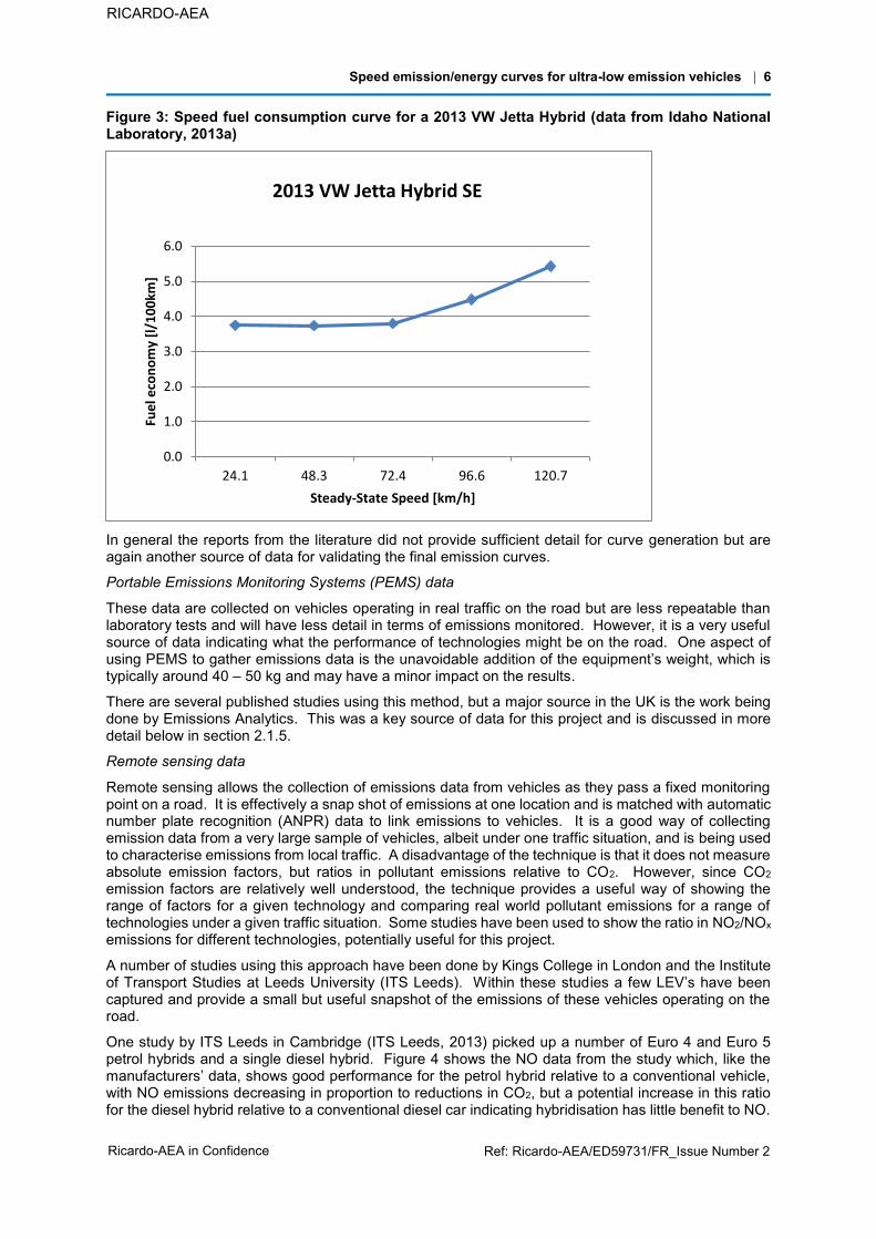
Data that can be used for this study include fuel consumption values for 2 electric vehicles at 8 average speeds (Idaho National Laboratory, 2014b), 4 hybrid electric vehicles at 5 average speeds (Idaho National Laboratory, 2013a), and 3 plug-in hybrid electric vehicles at 8 average speeds (Idaho National Laboratory, 2013b). An example of a speed curve for fuel consumption of an HEV is displayed below (Figure 3).
4 Mittelklassewagen = Medium sized car, Kleinwagen = Small sized car, Greenwagen = Green car, VKM = Combustion Engine, Hybrid, EV_opt = Optimal electric vehicle, CADC= Common Artemis Driving Cycles
0
20
40
60
80
100
120
140
Conventional Hybrid Plug-in hybrid Plug-inhybrid+RE
Electricvehicle
EV_Opt
CO
2em
issi
ons
(g C
O2/k
m)
Middle sized vehicle NEDC
Middle sized vehicle CADC
Small sized vehicle NEDC
Small sized vehicle CADC
Green vehicle NEDC
Green vehicle CADC
Speed emission/energy curves for ultra-low emission vehicles | 6
Ricardo-AEA in Confidence Ref: Ricardo-AEA/ED59731/FR_Issue Number 2
RICARDO-AEA
Figure 3: Speed fuel consumption curve for a 2013 VW Jetta Hybrid (data from Idaho National Laboratory, 2013a)
In general the reports from the literature did not provide sufficient detail for curve generation but are again another source of data for validating the final emission curves.
Portable Emissions Monitoring Systems (PEMS) data
These data are collected on vehicles operating in real traffic on the road but are less repeatable than laboratory tests and will have less detail in terms of emissions monitored. However, it is a very useful source of data indicating what the performance of technologies might be on the road. One aspect of using PEMS to gather emissions data is the unavoidable addition of the equipment’s weight, which is typically around 40 – 50 kg and may have a minor impact on the results.
There are several published studies using this method, but a major source in the UK is the work being done by Emissions Analytics. This was a key source of data for this project and is discussed in more detail below in section 2.1.5.
Remote sensing data
Remote sensing allows the collection of emissions data from vehicles as they pass a fixed monitoring point on a road. It is effectively a snap shot of emissions at one location and is matched with automatic number plate recognition (ANPR) data to link emissions to vehicles. It is a good way of collecting emission data from a very large sample of vehicles, albeit under one traffic situation, and is being used to characterise emissions from local traffic. A disadvantage of the technique is that it does not measure absolute emission factors, but ratios in pollutant emissions relative to CO2. However, since CO2 emission factors are relatively well understood, the technique provides a useful way of showing the range of factors for a given technology and comparing real world pollutant emissions for a range of technologies under a given traffic situation. Some studies have been used to show the ratio in NO2/NOx emissions for different technologies, potentially useful for this project.
A number of studies using this approach have been done by Kings College in London and the Institute of Transport Studies at Leeds University (ITS Leeds). Within these studies a few LEV’s have been captured and provide a small but useful snapshot of the emissions of these vehicles operating on the road.
One study by ITS Leeds in Cambridge (ITS Leeds, 2013) picked up a number of Euro 4 and Euro 5 petrol hybrids and a single diesel hybrid. Figure 4 shows the NO data from the study which, like the manufacturers’ data, shows good performance for the petrol hybrid relative to a conventional vehicle, with NO emissions decreasing in proportion to reductions in CO2, but a potential increase in this ratio for the diesel hybrid relative to a conventional diesel car indicating hybridisation has little benefit to NO.
0.0
1.0
2.0
3.0
4.0
5.0
6.0
24.1 48.3 72.4 96.6 120.7
Fue
l eco
no
my
[l/1
00
km]
Steady-State Speed [km/h]
2013 VW Jetta Hybrid SE

Speed emission/energy curves for ultra-low emission vehicles | 7
Ricardo-AEA in Confidence Ref: Ricardo-AEA/ED59731/FR_Issue Number 2
RICARDO-AEA
There is the added complication that for a hybrid vehicle it may be in full electric mode when it passes the detector. However, the lack of CO2 emissions to trigger the measurement will mean such events are systematically not counted.
Figure 4: NO emissions from a remote sensing study in Cambridge
Behaviour studies The key requirement of realistic emission estimation is a good prediction of real-world diving behaviour. The IFEU institute in Germany carried out a number of studies on this topic on electric and hybrid-electric vehicles. The most recent report on electric mobility (IFEU, 2014) deals with deriving typical behavioural patterns from a fleet test of VW TwinDrive diesel PHEVs and predicting their environmental impacts. Results show that emissions are highly dependent on the proportion of electric drive throughout the drive cycle.
To be able to represent the total contribution of grid electricity and conventional liquid fuels to the propulsion process the term ‘utility factor’ was introduced. The utility factor weights the consumption in each driving mode according to a modelled consumer behaviour that is based on travel survey data. Widely used standardized methods are the European ECE R101 method and the US SAE J2841 method. Several papers discuss the suitability of these existing utility factors and propose different approaches (Bradley and Quinn, 2010, Bradley and Davis, 2011, Baptista et al., 2012).
The concept of a utility factor will be particularly relevant to defining real-world emission factors for PHEVs under different driving situations or speeds by considering the mix of plug-in electric and combustion engine contributions to the vehicle propulsion. For the purposes of this study we adopted the standardised ECE R101 approach. However, there is scope for further work in this area to develop more behavioural based factors.
2.1.4 PHEM simulation data Overall the literature review provides useful background data on the emissions and energy use of low emission vehicles. However, it did not offer the real detail that is necessary to derive speed emission curves. Therefore we have used detailed simulations from the PHEM model to provide this data and validated this against the literature data.
The PHEM model was developed by the Technical University of Graz (TU Graz). It was originally an output of the EU ARTEMIS project which involved many of the leading transport research institutions in Europe. The model has subsequently been developed and maintained by TU Graz. ITS Leeds has worked closely with TU Graz in the use of this model.

Speed emission/energy curves for ultra-low emission vehicles | 8
Ricardo-AEA in Confidence Ref: Ricardo-AEA/ED59731/FR_Issue Number 2
RICARDO-AEA
The basic approach used by the PHEM model is to model the components of the vehicle in relation to a drive cycle in order to generate an engine speed/power (torque) profile. This is then related to an engine emission map generated on an engine test bed to provide engine out emissions. These can then be corrected by exhaust treatment modules to provide full vehicle emission results. This allows detailed modelling of vehicle technology combinations and vehicle drive cycles, from which emission results can be aggregated to give emission factors.
There are a number of vehicle configurations already set up with PHEM including a petrol hybrid passenger car, a conventional comparator and an electric vehicle. There are also a number of diesel cars that can be used for simulation work. The vehicle types used for simulation for this study were:
A petrol hybrid based on the VW Jetta hybrid and the comparator standard VW Jetta, which should reflect a typical petrol hybrid vehicle available today5;
The Peugeot Ion electric vehicle, being representative of a typical small EV; A Peugeot 5008 2.2l diesel vehicle used for comparison purposes with the PEMS data for the
Peugeot 5008 2.0l diesel hybrid described in section 2.1.5.
In addition to the main PHEM simulations ITS Leeds has developed, and made available a MatLab/Simulink model of the Nissan Leaf. This was used to provide additional data for the Nissan EV.
Simulation drive cycles The PHEM model takes drive cycle data in order to generate emission results for different driving conditions. The drive cycles are defined on a second-by-second basis and the emission results are generated on a second by second basis. The drive cycles used for the modelling include:
The London Drive Cycle developed by TfL representative of city driving; Worldwide harmonised Light vehicles Test Procedure (WLTP) giving a wider range of
conditions and being more representative of real world driving than the current regulation NEDC cycle. This drive cycle is still in draft as a regulatory test procedure but is currently due to be adopted by 2017.
These were chosen as they cover a range of driving conditions at different speeds. This allowed for the generation of data for deriving speed emission curves. The ‘London Drive Cycle’ (LDC) for example was developed for light-duty vehicles by TfL as part of an on-going Vehicle Emission Study. The drive cycle was developed in association with Millbrook, who were commissioned to track a car (VBox GPS and CAN Bus link) making repeated circuits of a set route in the North-East of London at different times of day: AM peak, Inter-peak and in Free-flow conditions. The route contained sections of (urban) motorway, suburban and urban (central London) driving conditions. Within these three road types there are three different traffic conditions: free-flowing, morning peak, and inter-peak for data collected between 10 am and 4 pm. These traffic conditions are abbreviated to “Free”, “Peak” and “IP”, e.g. as used in the x-axis of Figure 6.
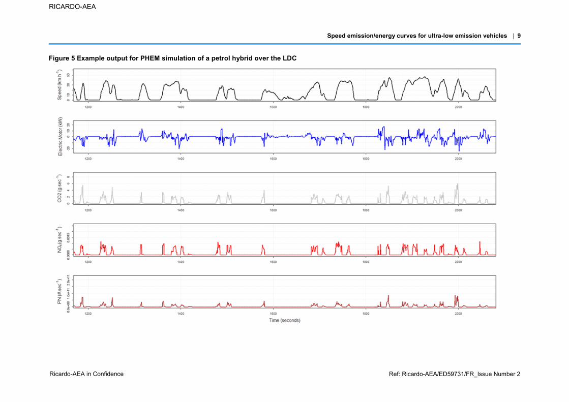
Example data from a PHEM simulation for a petrol hybrid over the LDC are shown in Figure 5 below. This shows second by second emissions results as well as other parameters that can be used such as vehicle speed and electrical motor power.
5 It is noted that the Jetta uses a Parallel P2 architecture, whereas the high volume sales (and widely used) Prius uses the Toyota Powersplit architecture.
Speed emission/energy curves for ultra-low emission vehicles | 9
Ricardo-AEA in Confidence Ref: Ricardo-AEA/ED59731/FR_Issue Number 2
RICARDO-AEA
Figure 5 Example output for PHEM simulation of a petrol hybrid over the LDC

Speed emission/energy curves for ultra-low emission vehicles | 10
Ricardo-AEA in Confidence Ref: Ricardo-AEA/ED59731/FR_Issue Number 2
RICARDO-AEA
Analysis of the simulation data The detailed data can be averaged for different segments of the drive cycle to provide average results for each segment as shown in Figure 6 below. However, in order to derive speed emission curves we have aggregated the second-by-second data into 1km/h speed bins. This data has then been used for curve fitting as shown in section 3.
Figure 6 NOx results by drive cycle segment for a hybrid and non-hybrid petrol car from PHEM
2.1.5 PEMS data from Emission Analytics PEMS data provide emission results from vehicles driven on-roads, using on-board emission measurement technology. Emissions Analytics is a leading provider of this data having tested hundreds of vehicles to provide real world data for consumers through organisations such as ‘What Car’. The data has focused on CO2 emissions and fuel consumption, but CO, NO and NO2 data are also collected. At present PM measurements are not made but the necessary technology to achieve this is being developed.
The data provide second by second emission results, similar in format to the PHEM simulation results, over an on-road drive cycle. The drive cycle is designed to cover a range of driving conditions and typically consists of:
An approximately 2 hour testing trip A mix of urban (average speed ~15mph) and extra-urban driving (~60mph) Maximum speed up to 70mph Drivers drive “normally”, which is judged by typical acceleration rates, no coasting, etc. Average acceleration rates are typically higher than NEDC, and involve less idling
Through this test programme Emission Analytics have tested a number of hybrid vehicles. Data from the following vehicles have been used in this study:
Peugeot 3008 2.0 diesel Peugeot 508 RXH 2.0 diesel Mercedes-Benz E300 2143 cc diesel6 Volvo V60 2.4 diesel plug-in Mitsubishi Outlander 2.0 gasoline plug-in
6 This Mercedes Benz hybrid is referred to both as a 2.1 and 2.2 litre engine. In this report, e.g. in Figure 13 it is referred to as a 2.2 litre engine.
Speed emission/energy curves for ultra-low emission vehicles | 11
Ricardo-AEA in Confidence Ref: Ricardo-AEA/ED59731/FR_Issue Number 2
RICARDO-AEA
Toyota Prius 1.8 gasoline The focus of the vehicles selected was on diesel hybrids as this is the vehicle group where least data were available from the literature and for which a PHEM simulation was not possible. Two petrol hybrids were also included to validate the petrol hybrid PHEM simulation results.
The PEMS data were analysed in exactly the same way as the PHEM results. The second-by-second data were aggregate in 1kph speed bins to allow for curve fitting. The results are described in section 3.
2.1.6 Data for heavy duty vehicles Most of the data found in this review has been for light duty LEVs. Previous work carried out for Defra in 2013 reviewed air pollutant emissions from methane-fuelled HGVs and buses (Ricardo-AEA, 2013). The study reviewed available evidence from the literature and from consultation with stakeholders, including the Low Carbon Vehicle Partnership. The study differentiated emissions from dedicated methane vehicles equipped with three-way catalysts from dual-fuel methane-diesel vehicles. The main conclusion from the review was that the former showed good reductions in NOx and PM emissions relative to a diesel equivalent vehicle, but that there was insufficient evidence to conclude impacts from dual-fuel vehicles. This is important because dual fuel vehicles could become more common, with eleven of the thirteen DfT Innovate UK funded projects in the “Low carbon truck demonstration trial” using dual fuel technology.
Further evidence has become available since our 2013 review for Defra, in particular the following sources:
Recently published literature and manufacturers’ publicity; DfT Low Carbon Truck and Refuelling Infrastructure Demonstration Trial (for dual fuel
vehicles); DfT Methane slip test protocol study (data for a single dedicated rigid methane truck and a
single dual fuel articulated truck).
These data provide the foundation of the evidence base used to develop the required speed curves for dedicated methane rigid trucks and dual fuel articulated trucks. Speed curves for dedicated methane articulated trucks and dual fuel rigid trucks were obtained by extrapolation.
For battery operated trucks there is a limited amount of data available.
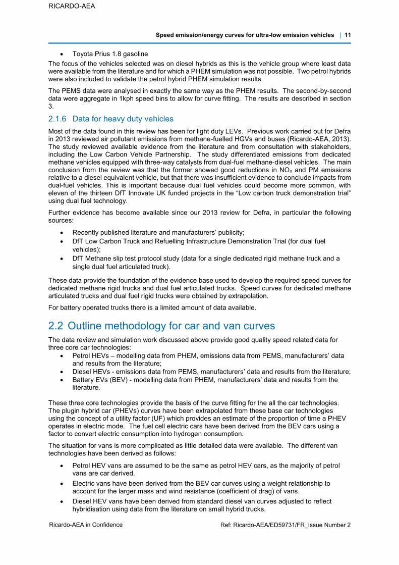
2.2 Outline methodology for car and van curves The data review and simulation work discussed above provide good quality speed related data for three core car technologies:
Petrol HEVs – modelling data from PHEM, emissions data from PEMS, manufacturers’ data and results from the literature;
Diesel HEVs - emissions data from PEMS, manufacturers’ data and results from the literature; Battery EVs (BEV) - modelling data from PHEM, manufacturers’ data and results from the
literature. These three core technologies provide the basis of the curve fitting for the all the car technologies. The plugin hybrid car (PHEVs) curves have been extrapolated from these base car technologies using the concept of a utility factor (UF) which provides an estimate of the proportion of time a PHEV operates in electric mode. The fuel cell electric cars have been derived from the BEV cars using a factor to convert electric consumption into hydrogen consumption.
The situation for vans is more complicated as little detailed data were available. The different van technologies have been derived as follows:
Petrol HEV vans are assumed to be the same as petrol HEV cars, as the majority of petrol vans are car derived.
Electric vans have been derived from the BEV car curves using a weight relationship to account for the larger mass and wind resistance (coefficient of drag) of vans.
Diesel HEV vans have been derived from standard diesel van curves adjusted to reflect hybridisation using data from the literature on small hybrid trucks.
Speed emission/energy curves for ultra-low emission vehicles | 12
Ricardo-AEA in Confidence Ref: Ricardo-AEA/ED59731/FR_Issue Number 2
RICARDO-AEA
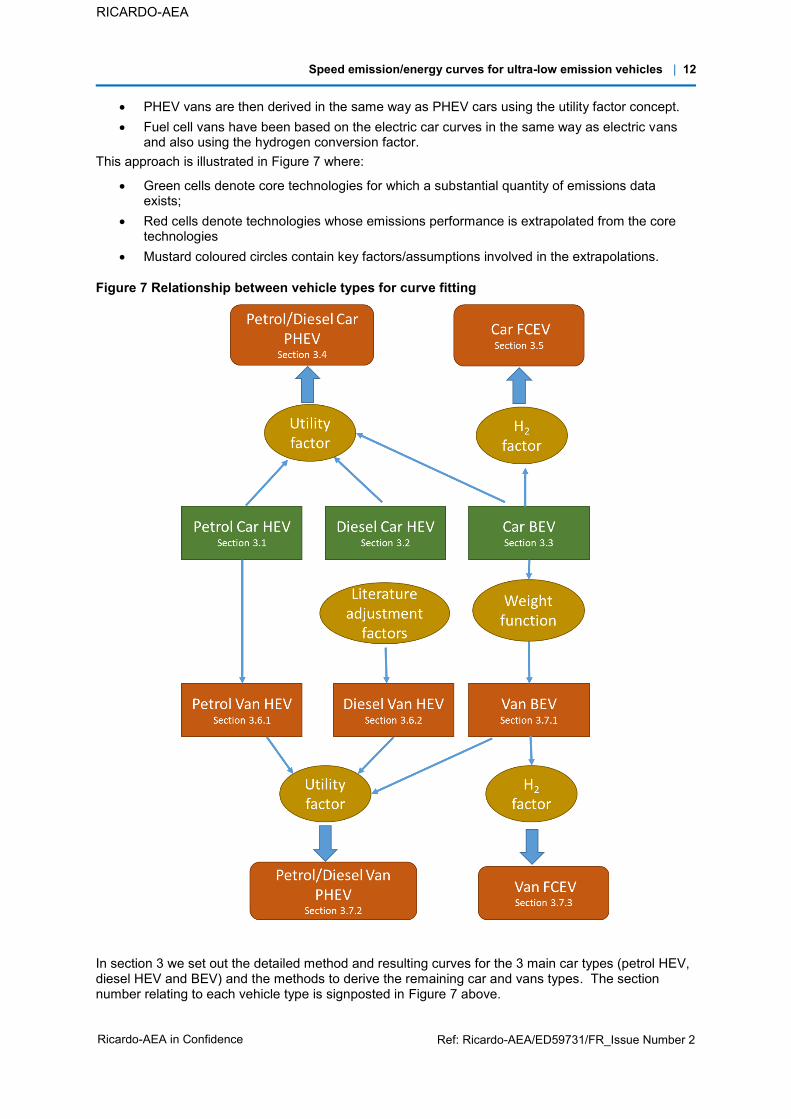
PHEV vans are then derived in the same way as PHEV cars using the utility factor concept. Fuel cell vans have been based on the electric car curves in the same way as electric vans
and also using the hydrogen conversion factor. This approach is illustrated in Figure 7 where:
Green cells denote core technologies for which a substantial quantity of emissions data exists;
Red cells denote technologies whose emissions performance is extrapolated from the core technologies
Mustard coloured circles contain key factors/assumptions involved in the extrapolations.
Figure 7 Relationship between vehicle types for curve fitting
In section 3 we set out the detailed method and resulting curves for the 3 main car types (petrol HEV, diesel HEV and BEV) and the methods to derive the remaining car and vans types. The section number relating to each vehicle type is signposted in Figure 7 above.
Speed emission/energy curves for ultra-low emission vehicles | 13
Ricardo-AEA in Confidence Ref: Ricardo-AEA/ED59731/FR_Issue Number 2
RICARDO-AEA
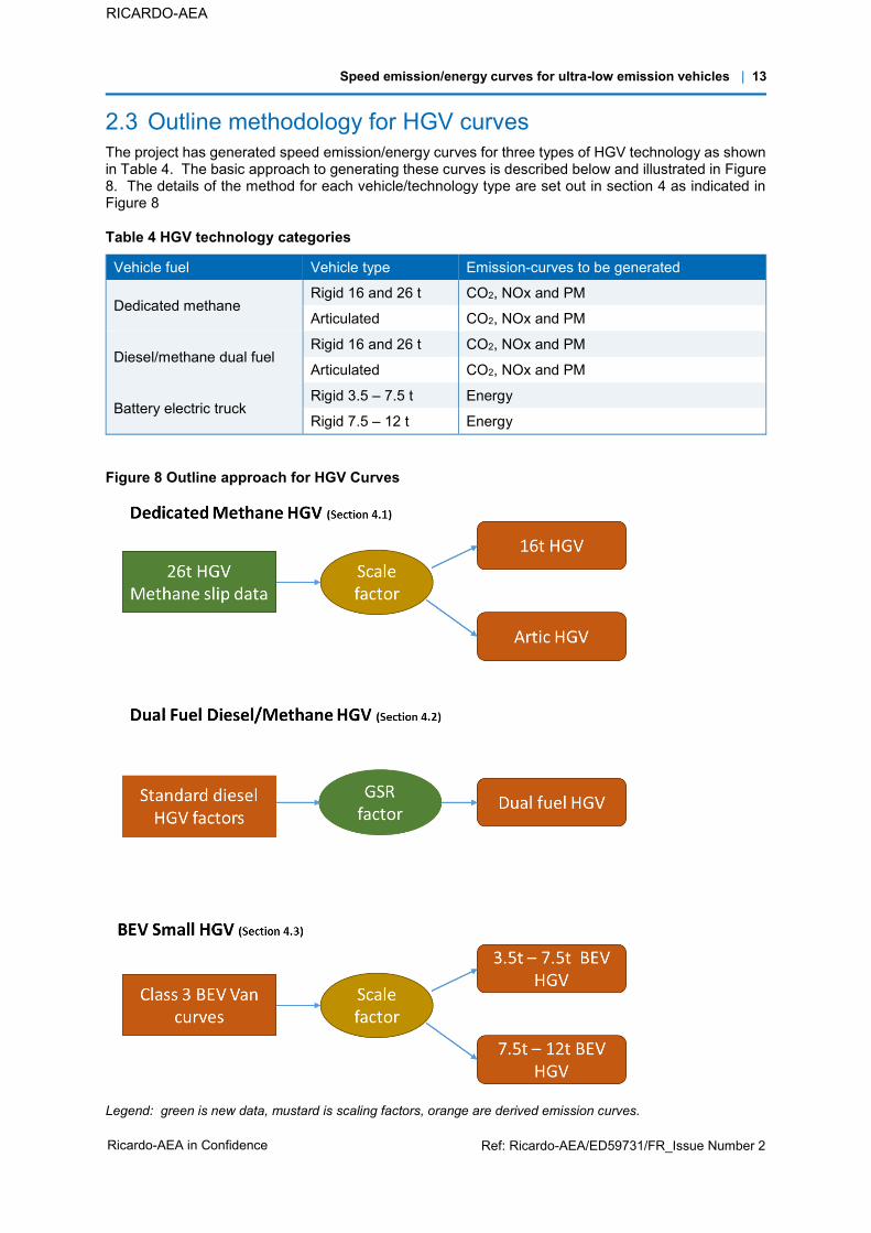
2.3 Outline methodology for HGV curves The project has generated speed emission/energy curves for three types of HGV technology as shown in Table 4. The basic approach to generating these curves is described below and illustrated in Figure 8. The details of the method for each vehicle/technology type are set out in section 4 as indicated in Figure 8
Table 4 HGV technology categories
Vehicle fuel Vehicle type Emission-curves to be generated
Dedicated methane Rigid 16 and 26 t CO2, NOx and PM
Articulated CO2, NOx and PM
Diesel/methane dual fuel Rigid 16 and 26 t CO2, NOx and PM
Articulated CO2, NOx and PM
Battery electric truck Rigid 3.5 – 7.5 t Energy
Rigid 7.5 – 12 t Energy
Figure 8 Outline approach for HGV Curves
Legend: green is new data, mustard is scaling factors, orange are derived emission curves.

Speed emission/energy curves for ultra-low emission vehicles | 14
Ricardo-AEA in Confidence Ref: Ricardo-AEA/ED59731/FR_Issue Number 2
RICARDO-AEA
2.3.1 Dedicated methane fuelled HGV The Ricardo-AEA (2013) study reviewed the reported emissions for dedicated methane fuelled HGV and provided emissions factors for 16 tonne rigid trucks for NOx, PM and CO2, expressed in units of g/km. Reviewing these data for this study identified the following gaps:
The emission factors given are average factors, not speed-related emission factors, Emission factors for the less common articulated trucks are not provided.
Further work in this study has identified data in order to fill these gaps. The source of data used has been the real world test data for a dedicated methane HGV tested as part of the DfT methane slip project. These data were used to generate speed-emission curves for CO2 and NOx for a 26t rigid vehicle. There was not further data on PM emissions but since these are very low the existing non-speed dependent PM factor derived from the 2013 Ricardo-AEA study has been retained.
The curves derived for the 26t rigid vehicle have been used as the basis for extrapolating curves for a 16t rigid and an articulated vehicle. The details of the extrapolation are provided in section 4.
2.3.2 Methane/diesel dual fuel HGV The Ricardo-AEA (2013) report to Defra noted: “There was extremely little evidence available for dual fuel methane-diesel vehicles. This is a notable gap in vehicle emissions data. The absence of data means this project cannot recommend emission factors for dual fuel methane-diesel vehicles.”
However, since that review was undertaken a number of studies have been published, and some preliminary data has been obtained from the Low Carbon Truck Demonstration trial and the DfT Methane slip project. Although these data are still not sufficient direct evidence of the relationship between speed and emissions, the data collected did provide information on:
the difference between dual and diesel operation over whole test cycles; the relationship between emissions and gas substitution ratio (GSR); the relationship between GSR and average speed.
Using these data speed-emission curves were derived as discussed in section 4.
2.3.3 BEV trucks Speed-energy curves for the smaller BEV trucks have been extrapolated from the BEV van curves for class 3 vans, as discussed in section 4.
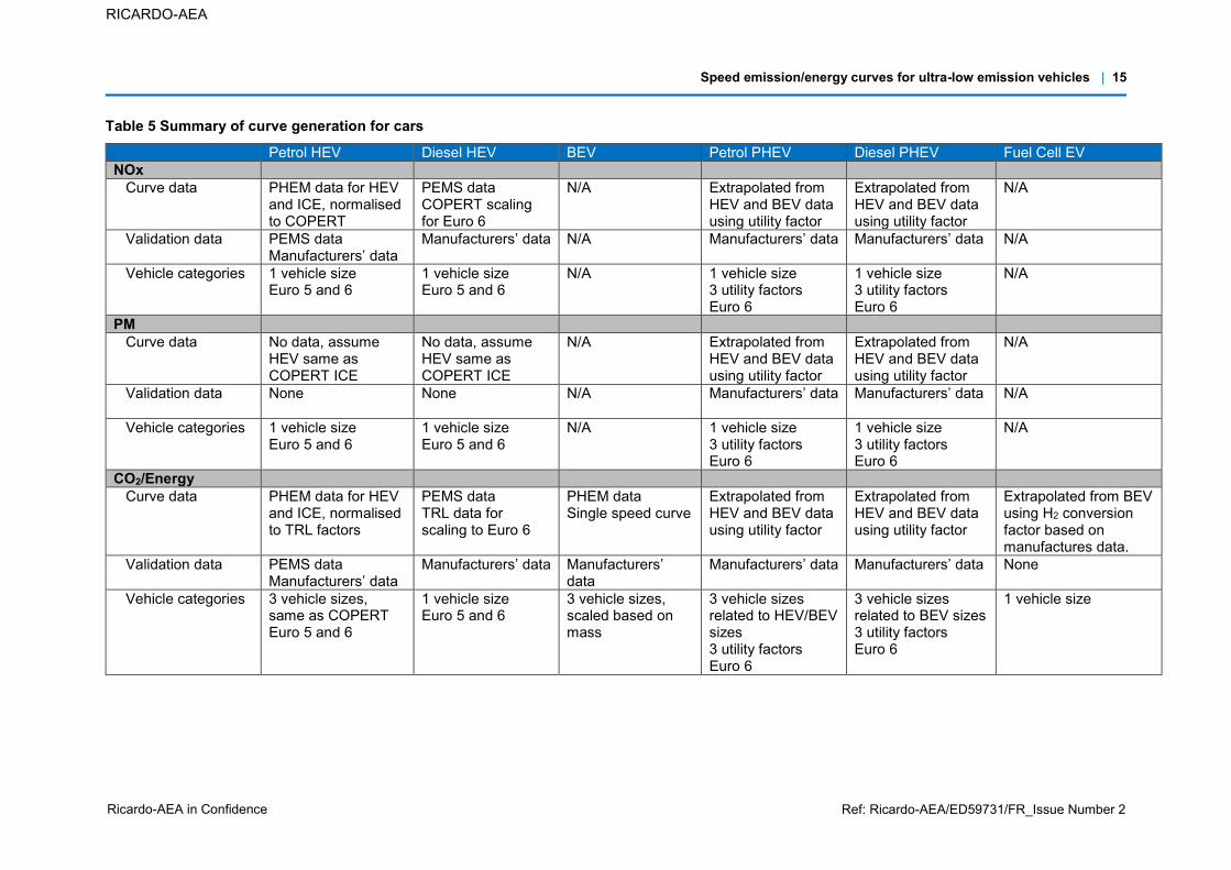
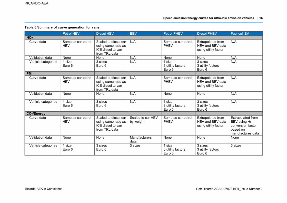
2.4 Summary data and method tables The overall approach to the curve generation for each vehicle type and pollutant is summarised in Table 5 and Table 6 below. For each pollutant and vehicle type the tables provide details on:
Curve data – the data source that was used to generate the curve. Validation data – the data that was used to validate the curve to ensure that it is generating
reliable results. Vehicle categories – the level of disaggregation of the vehicle type, in terms of individual curves,
relating to vehicle size and Euro standard.
The key aspects of the approach taken for main vehicle types cars, vans and HGVs are as follows:
Cars – the car curves are based on modelled data from PHEM and measured PEMS data, giving us a robust and validated set of curves.
Vans – no direct data were available for these and so they have been extrapolated from the car data using literature results and scaling based on weight and power.
HGV – this is based on a mixture of literature results and some measured data.
Speed emission/energy curves for ultra-low emission vehicles | 15
Ricardo-AEA in Confidence Ref: Ricardo-AEA/ED59731/FR_Issue Number 2
RICARDO-AEA
Table 5 Summary of curve generation for cars
Petrol HEV Diesel HEV BEV Petrol PHEV Diesel PHEV Fuel Cell EV NOx Curve data PHEM data for HEV
and ICE, normalised to COPERT
PEMS data COPERT scaling for Euro 6
N/A Extrapolated from HEV and BEV data using utility factor
Extrapolated from HEV and BEV data using utility factor
N/A
Validation data PEMS data Manufacturers’ data
Manufacturers’ data N/A Manufacturers’ data Manufacturers’ data N/A
Vehicle categories 1 vehicle size Euro 5 and 6
1 vehicle size Euro 5 and 6
N/A 1 vehicle size 3 utility factors Euro 6
1 vehicle size 3 utility factors Euro 6
N/A
PM Curve data No data, assume
HEV same as COPERT ICE
No data, assume HEV same as COPERT ICE
N/A Extrapolated from HEV and BEV data using utility factor
Extrapolated from HEV and BEV data using utility factor
N/A
Validation data
None None N/A Manufacturers’ data Manufacturers’ data N/A
Vehicle categories 1 vehicle size Euro 5 and 6
1 vehicle size Euro 5 and 6
N/A 1 vehicle size 3 utility factors Euro 6
1 vehicle size 3 utility factors Euro 6
N/A
CO2/Energy Curve data PHEM data for HEV
and ICE, normalised to TRL factors
PEMS data TRL data for scaling to Euro 6
PHEM data Single speed curve
Extrapolated from HEV and BEV data using utility factor
Extrapolated from HEV and BEV data using utility factor
Extrapolated from BEV using H2 conversion factor based on manufactures data.
Validation data PEMS data Manufacturers’ data
Manufacturers’ data Manufacturers’ data
Manufacturers’ data Manufacturers’ data None
Vehicle categories 3 vehicle sizes, same as COPERT Euro 5 and 6
1 vehicle size Euro 5 and 6
3 vehicle sizes, scaled based on mass
3 vehicle sizes related to HEV/BEV sizes 3 utility factors Euro 6
3 vehicle sizes related to BEV sizes 3 utility factors Euro 6
1 vehicle size
Speed emission/energy curves for ultra-low emission vehicles | 16
Ricardo-AEA in Confidence Ref: Ricardo-AEA/ED59731/FR_Issue Number 2
RICARDO-AEA
Table 6 Summary of curve generation for vans Petrol HEV Diesel HEV BEV Petrol PHEV Diesel PHEV Fuel cell EV NOx Curve data Same as car petrol
HEV Scaled to diesel car using same ratio as ICE diesel to van from TRL data
N/A Same as car petrol PHEV
Extrapolated from HEV and BEV data using utility factor
N/A
Validation data None None N/A None None N/A Vehicle categories 1 size
Euro 6 3 sizes Euro 6
N/A 1 size 3 utility factors Euro 6
3 sizes 3 utility factors Euro 6
N/A
PM Curve data Same as car petrol
HEV Scaled to diesel car using same ratio as ICE diesel to van from TRL data
N/A Same as car petrol PHEV
Extrapolated from HEV and BEV data using utility factor
N/A
Validation data
None None N/A None None N/A
Vehicle categories 1 size Euro 6
3 sizes Euro 6
N/A 1 size 3 utility factors Euro 6
3 sizes 3 utility factors Euro 6
N/A
CO2/Energy Curve data Same as car petrol
HEV Scaled to diesel car using same ratio as ICE diesel to van from TRL data
Scaled to car HEV by weight
Same as car petrol PHEV
Extrapolated from HEV and BEV data using utility factor
Extrapolated from BEV using H2 conversion factor based on manufactures data
Validation data None None Manufacturers’ data
None None None
Vehicle categories 1 size Euro 6
3 sizes Euro 6
3 sizes 1 size 3 utility factors Euro 6
3 sizes 3 utility factors Euro 6
3 sizes
Speed emission/energy curves for ultra-low emission vehicles | 17
Ricardo-AEA in Confidence Ref: Ricardo-AEA/ED59731/FR_Issue Number 2
RICARDO-AEA
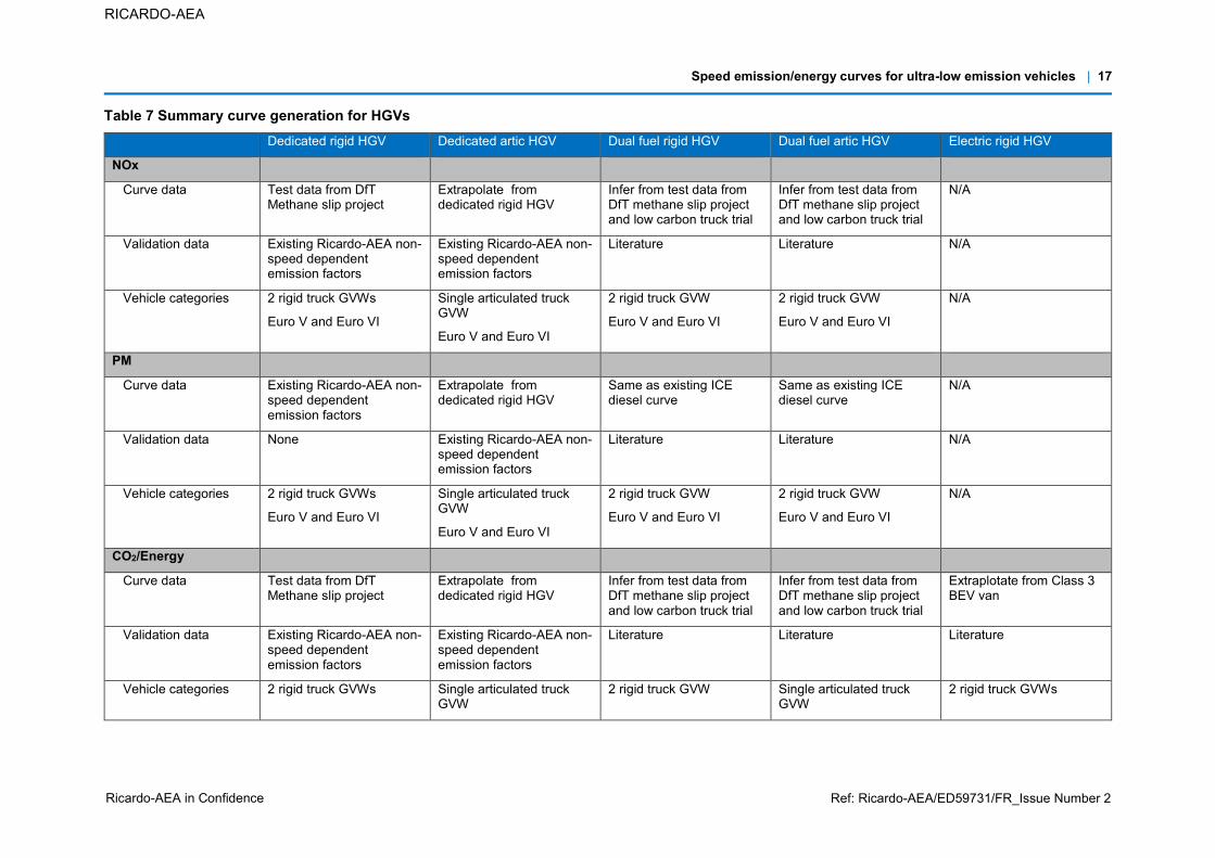
Table 7 Summary curve generation for HGVs Dedicated rigid HGV Dedicated artic HGV Dual fuel rigid HGV Dual fuel artic HGV Electric rigid HGV
NOx
Curve data Test data from DfT Methane slip project
Extrapolate from dedicated rigid HGV
Infer from test data from DfT methane slip project and low carbon truck trial
Infer from test data from DfT methane slip project and low carbon truck trial
N/A
Validation data Existing Ricardo-AEA non-speed dependent emission factors
Existing Ricardo-AEA non-speed dependent emission factors
Literature Literature N/A
Vehicle categories 2 rigid truck GVWs
Euro V and Euro VI
Single articulated truck GVW
Euro V and Euro VI
2 rigid truck GVW
Euro V and Euro VI
2 rigid truck GVW
Euro V and Euro VI
N/A
PM
Curve data Existing Ricardo-AEA non-speed dependent emission factors
Extrapolate from dedicated rigid HGV
Same as existing ICE diesel curve
Same as existing ICE diesel curve
N/A
Validation data
None Existing Ricardo-AEA non-speed dependent emission factors
Literature Literature N/A
Vehicle categories 2 rigid truck GVWs
Euro V and Euro VI
Single articulated truck GVW
Euro V and Euro VI
2 rigid truck GVW
Euro V and Euro VI
2 rigid truck GVW
Euro V and Euro VI
N/A
CO2/Energy
Curve data Test data from DfT Methane slip project
Extrapolate from dedicated rigid HGV
Infer from test data from DfT methane slip project and low carbon truck trial
Infer from test data from DfT methane slip project and low carbon truck trial
Extraplotate from Class 3 BEV van
Validation data Existing Ricardo-AEA non-speed dependent emission factors
Existing Ricardo-AEA non-speed dependent emission factors
Literature Literature Literature
Vehicle categories 2 rigid truck GVWs Single articulated truck GVW
2 rigid truck GVW Single articulated truck GVW
2 rigid truck GVWs
Speed emission/energy curves for ultra-low emission vehicles | 18
Ricardo-AEA in Confidence Ref: Ricardo-AEA/ED59731/FR_Issue Number 2
RICARDO-AEA
3 Emission curves for cars and vans The detailed analysis and results for each of the car and van technologies is set out in the following sections. The first three sections deal with the core car technologies, petrol HEV, diesel HEV and BEV, for which we had detailed speed related data. The remaining sections detail the extrapolation approach used for the remaining car types and the van types where there is much less data available.
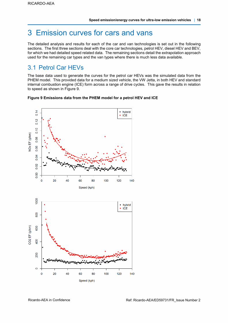
3.1 Petrol Car HEVs The base data used to generate the curves for the petrol car HEVs was the simulated data from the PHEM model. This provided data for a medium sized vehicle, the VW Jetta, in both HEV and standard internal combustion engine (ICE) form across a range of drive cycles. This gave the results in relation to speed as shown in Figure 9.
Figure 9 Emissions data from the PHEM model for a petrol HEV and ICE
Speed emission/energy curves for ultra-low emission vehicles | 19
Ricardo-AEA in Confidence Ref: Ricardo-AEA/ED59731/FR_Issue Number 2
RICARDO-AEA
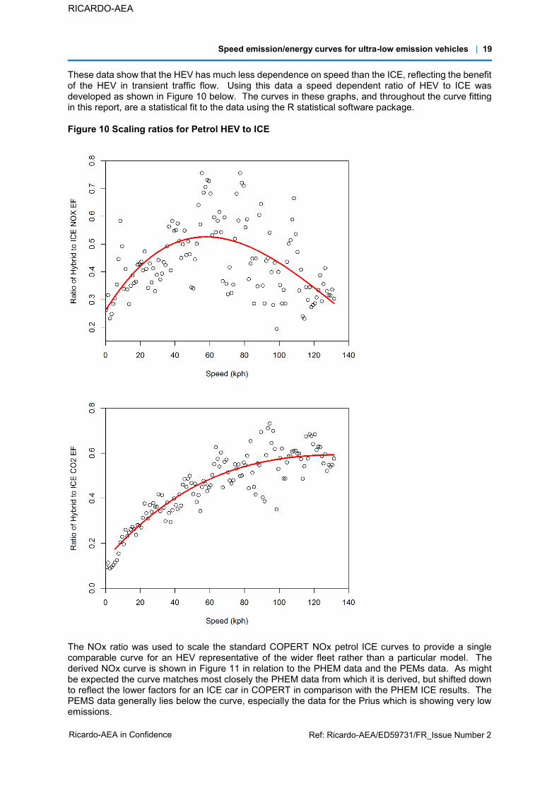
These data show that the HEV has much less dependence on speed than the ICE, reflecting the benefit of the HEV in transient traffic flow. Using this data a speed dependent ratio of HEV to ICE was developed as shown in Figure 10 below. The curves in these graphs, and throughout the curve fitting in this report, are a statistical fit to the data using the R statistical software package.
Figure 10 Scaling ratios for Petrol HEV to ICE
The NOx ratio was used to scale the standard COPERT NOx petrol ICE curves to provide a single comparable curve for an HEV representative of the wider fleet rather than a particular model. The derived NOx curve is shown in Figure 11 in relation to the PHEM data and the PEMs data. As might be expected the curve matches most closely the PHEM data from which it is derived, but shifted down to reflect the lower factors for an ICE car in COPERT in comparison with the PHEM ICE results. The PEMS data generally lies below the curve, especially the data for the Prius which is showing very low emissions.

Speed emission/energy curves for ultra-low emission vehicles | 20
Ricardo-AEA in Confidence Ref: Ricardo-AEA/ED59731/FR_Issue Number 2
RICARDO-AEA
The CO2 ratio was used with the TRL Euro 5 petrol ICE curves to provide the CO2 curves for three car sizes. The curve for a medium car is shown in Figure 12 against the PHEM and PEMS data. In this case both the PHEM and PEMS data lie above the curve, so the derived curve is under estimating CO2 to some degree. This suggests that the existing TRL CO2 curve, which we are scaling, is rather optimistic for current ICE vehicles. However, this approach does mean that the derived curves are consistent with the existing ICE curves used in the NTM in relative terms, but in the longer term the existing ICE curves may need to be revisited.
Figure 11 Derived petrol HEV NOx curve against PHEM and PEMS data
Figure 12 Derived petrol HEV CO2 curve against PHEM and PEMS data
Speed emission/energy curves for ultra-low emission vehicles | 21
Ricardo-AEA in Confidence Ref: Ricardo-AEA/ED59731/FR_Issue Number 2
RICARDO-AEA
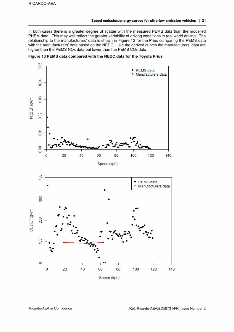
In both cases there is a greater degree of scatter with the measured PEMS data than the modelled PHEM data. This may well reflect the greater variability of driving conditions in real world driving. The relationship to the manufacturers’ data is shown in Figure 13 for the Prius comparing the PEMS data with the manufacturers’ data based on the NEDC. Like the derived curves the manufacturers’ data are higher than the PEMS NOx data but lower than the PEMS CO2 data.
Figure 13 PEMS data compared with the NEDC data for the Toyota Prius

Speed emission/energy curves for ultra-low emission vehicles | 22
Ricardo-AEA in Confidence Ref: Ricardo-AEA/ED59731/FR_Issue Number 2
RICARDO-AEA
Foth both NOx and CO2 the curves have been derived from Euro 5 data. To get the Euro 6 curves, the Euro 5 curves have simply been scaled by the same ratio as the Euro 6/Euro 5 ratio for ICE COPERT curves, although it should be noted that the ratio for NOx is 1.
There were no readily available speed related PM data for the petrol HEVs. However, since PM emissions are very low from petrol vehicles it is our proposal to simply use the same PM curves as for conventional petrol ICEs
3.2 Diesel HEV cars The simulation exercise for the diesel HEVs did not provide credible data as it was not based on a direct simulation but an extrapolation. Therefore the curve fitting exercise was carried out with the measured PEMS data that were available for 3 diesel HEVs. The data for NOx and CO2 are shown below in Figure 14 and Figure 16. Also since we did not have comparator ICE diesel data an initial comparison was carried out with the existing ICE diesel emissions curves for a large car. The large diesel ICE was selected as all the HEV vehicles were relatively large and used 2.0 or 2.2l diesel engines. These are all for Euro 5 vehicles.
Figure 14 Diesel car HEV PEMS NOx data
For the NOx data there was a fair degree of scatter in the results and no discernible speed dependence (as illustrated is the flat fit line). The comparison of the fit line against the Euro 5 COPERT diesel curve, suggests that at most speeds the HEV is producing more NOx than the ICE. This is generally consistent with the manufacturers’ data that was reviewed during the initial data task and shown in Figure 15.
Speed emission/energy curves for ultra-low emission vehicles | 23
Ricardo-AEA in Confidence Ref: Ricardo-AEA/ED59731/FR_Issue Number 2
RICARDO-AEA
Figure 15 Manufacture’s NOx data for the diesel HEVs assessed
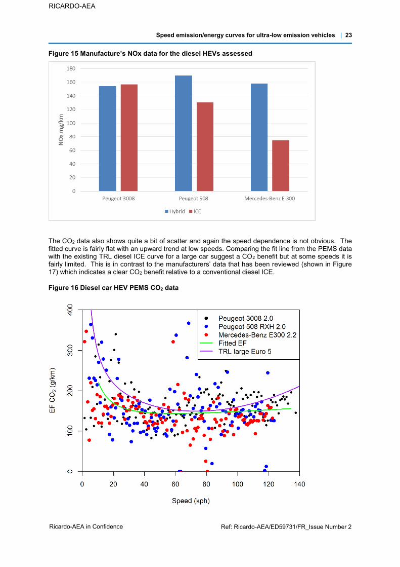
The CO2 data also shows quite a bit of scatter and again the speed dependence is not obvious. The fitted curve is fairly flat with an upward trend at low speeds. Comparing the fit line from the PEMS data with the existing TRL diesel ICE curve for a large car suggest a CO2 benefit but at some speeds it is fairly limited. This is in contrast to the manufacturers’ data that has been reviewed (shown in Figure 17) which indicates a clear CO2 benefit relative to a conventional diesel ICE.
Figure 16 Diesel car HEV PEMS CO2 data
Speed emission/energy curves for ultra-low emission vehicles | 24
Ricardo-AEA in Confidence Ref: Ricardo-AEA/ED59731/FR_Issue Number 2
RICARDO-AEA
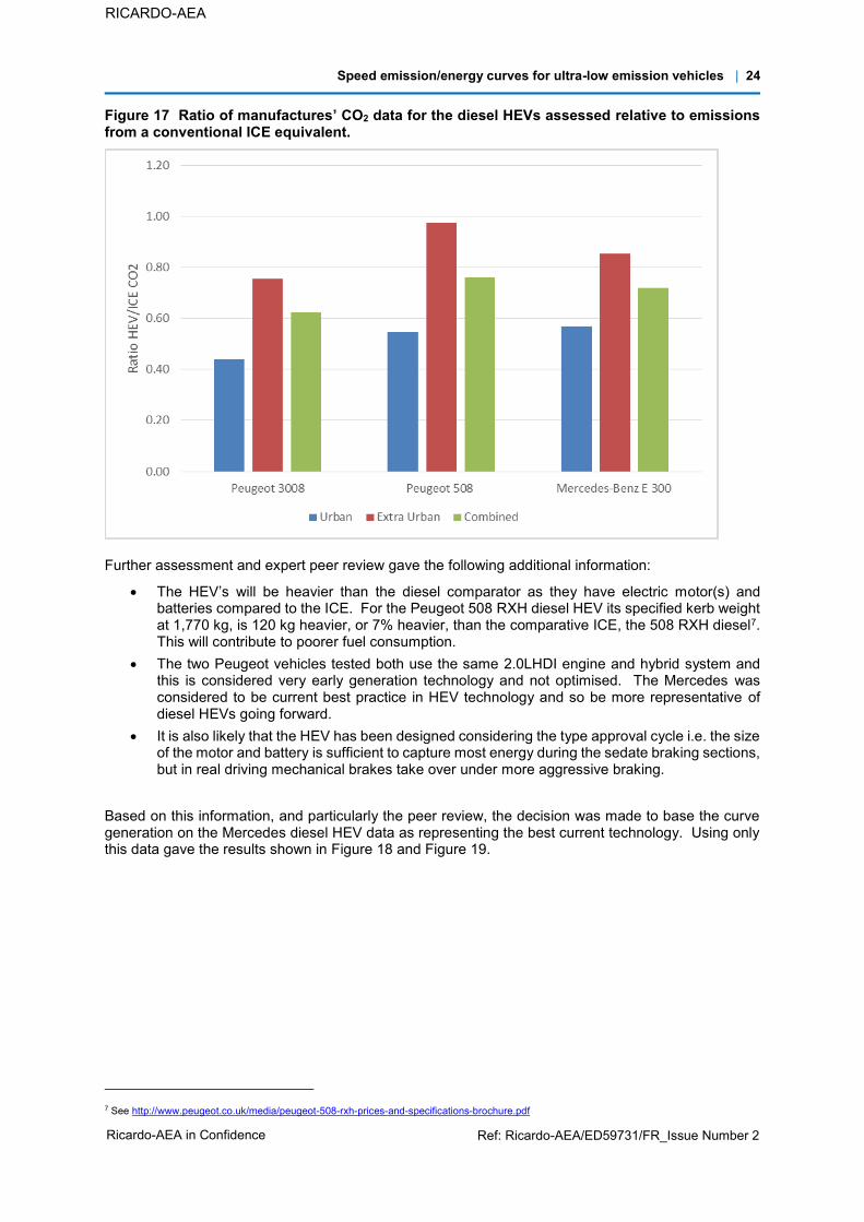
Figure 17 Ratio of manufactures’ CO2 data for the diesel HEVs assessed relative to emissions from a conventional ICE equivalent.
Further assessment and expert peer review gave the following additional information:
The HEV’s will be heavier than the diesel comparator as they have electric motor(s) and batteries compared to the ICE. For the Peugeot 508 RXH diesel HEV its specified kerb weight at 1,770 kg, is 120 kg heavier, or 7% heavier, than the comparative ICE, the 508 RXH diesel7. This will contribute to poorer fuel consumption.
The two Peugeot vehicles tested both use the same 2.0LHDI engine and hybrid system and this is considered very early generation technology and not optimised. The Mercedes was considered to be current best practice in HEV technology and so be more representative of diesel HEVs going forward.
It is also likely that the HEV has been designed considering the type approval cycle i.e. the size of the motor and battery is sufficient to capture most energy during the sedate braking sections, but in real driving mechanical brakes take over under more aggressive braking.
Based on this information, and particularly the peer review, the decision was made to base the curve generation on the Mercedes diesel HEV data as representing the best current technology. Using only this data gave the results shown in Figure 18 and Figure 19.
7 See http://www.peugeot.co.uk/media/peugeot-508-rxh-prices-and-specifications-brochure.pdf

Speed emission/energy curves for ultra-low emission vehicles | 25
Ricardo-AEA in Confidence Ref: Ricardo-AEA/ED59731/FR_Issue Number 2
RICARDO-AEA
Figure 18 Diesel HEV NOx curve from Mercedes data
Figure 19 Diesel HEV CO2 curve from Mercedes data
The derived NOx curve is now showing a speed dependence and is indicating a NOx saving at low speeds compared to the ICE, but a NOx penalty at speeds above 40kph. On average across the speed range the HEV has a 25% increase in NOx emissions over the ICE. With the CO2 curve the Mercedes data are showing a more consistent benefit over the ICE compared to the data from all the PEMs results. On average the HEV is showing an 18% CO2 saving. For NOx, all of the data are higher than the manufacturers’ NOx figures showing the impact of real world driving over the NEDC test.

Speed emission/energy curves for ultra-low emission vehicles | 26
Ricardo-AEA in Confidence Ref: Ricardo-AEA/ED59731/FR_Issue Number 2
RICARDO-AEA
There are no comparative PEMS data for a diesel ICE car so for both NOx and CO2 the curves derived are based purely on the PEMS data and not normalised back to COPERT or TRL as was done for the petrol HEV cars. These provide the Euro 5 curves and, as with the petrol vehicles, these have been scaled to Euro 6 using the ratio for Euro 6/Euro 5 from the COPERT curves for NOx and TRL curves for CO2 for ICE cars. For diesel cars, Euro 6 is essentially being introduced in two stages, the second (Euro 6c) in 2018. The emission limits are the same for both stages, but Euro 6c will involve a different test procedure which should lead to lower ‘real world’ emission factors. The NAEI is currently reviewing new factors for Euro 6 and Euro 6c given in the latest version of COPERT 4 v11. However, since the reductions in factors for Euro 6c are not included in the emission curves for conventional ICE diesel cars provided for the NTM in 2013/14, these have not been included in the factors for diesel HEVs so that the emission curves for both these vehicles remain comparable. A space for Euro 6c has been provided in the aggregation spreadsheet for inclusion at a later stage and we recommend this is done when the curves for diesel ICE cars are updated.
As with the petrol HEVs there were no PM data available. Since both HEV and ICE cars at Euro 5 and 6 will be fitted with diesel particulate filters (DPFs) which are highly efficient it has been assumed that the HEV PM emissions will be the same as the low values for the ICE.
3.3 Battery electric vehicles (BEVs) Two battery electric vehicles have been simulated to derive speed/energy data. These were the Peugeot Ion and the Nissan Leaf. The Ion was modelled in PHEM and the Leaf in a bespoke MatLab/Simulink simulation. The results are shown in Figure 20 below and are expressed in kWh/km in terms of energy demand on the battery. These data show a clear speed dependence and it is consistent for both vehicle models. We have therefore taken the curve fitted to the Ion to provide a representative curve for the BEVs. The Ion was chosen rather than the Leaf as it was simulated with PHEM and hence is consistent with the other simulation work done in the project. However, the consistency with the Leaf provides validation of the BEV curve shape for use with EV’s larger than the Ion.
Figure 20 Simulated energy use data for the Peugeot Ion and Nissan Leaf
Speed emission/energy curves for ultra-low emission vehicles | 27
Ricardo-AEA in Confidence Ref: Ricardo-AEA/ED59731/FR_Issue Number 2
RICARDO-AEA
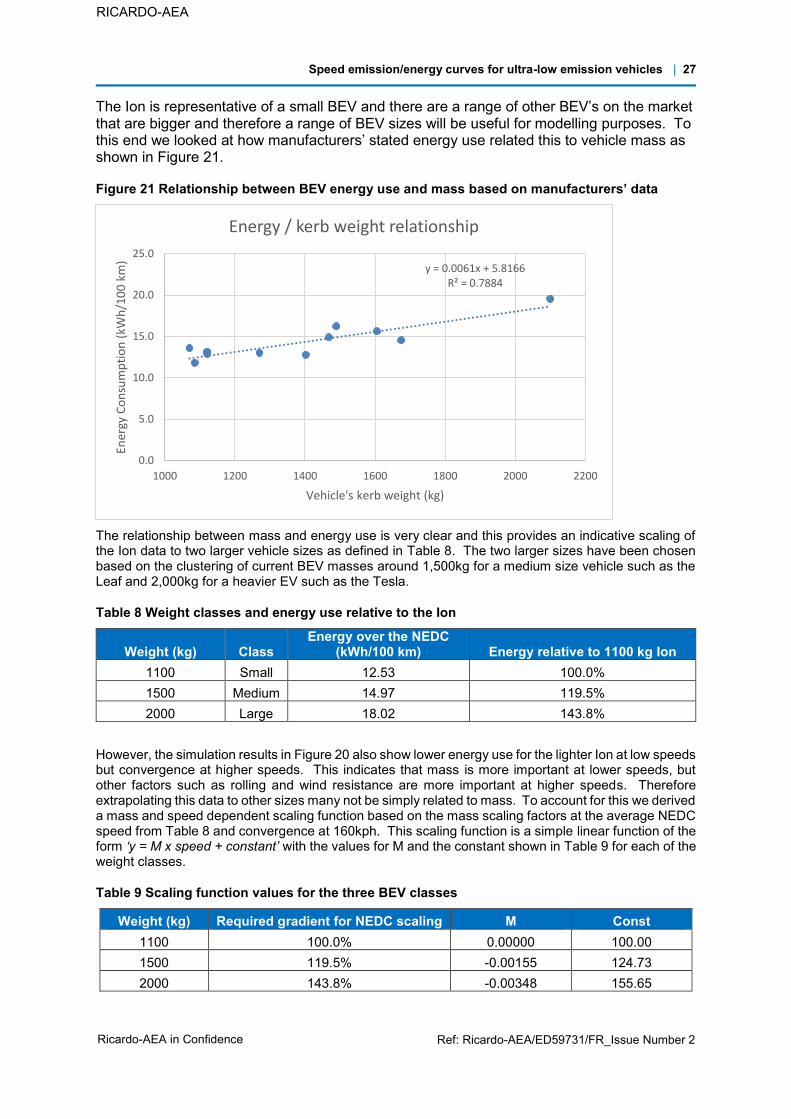
The Ion is representative of a small BEV and there are a range of other BEV’s on the market that are bigger and therefore a range of BEV sizes will be useful for modelling purposes. To this end we looked at how manufacturers’ stated energy use related this to vehicle mass as shown in Figure 21.
Figure 21 Relationship between BEV energy use and mass based on manufacturers’ data
The relationship between mass and energy use is very clear and this provides an indicative scaling of the Ion data to two larger vehicle sizes as defined in Table 8. The two larger sizes have been chosen based on the clustering of current BEV masses around 1,500kg for a medium size vehicle such as the Leaf and 2,000kg for a heavier EV such as the Tesla.
Table 8 Weight classes and energy use relative to the Ion
Weight (kg) Class Energy over the NEDC
(kWh/100 km) Energy relative to 1100 kg Ion 1100 Small 12.53 100.0% 1500 Medium 14.97 119.5% 2000 Large 18.02 143.8%
However, the simulation results in Figure 20 also show lower energy use for the lighter Ion at low speeds but convergence at higher speeds. This indicates that mass is more important at lower speeds, but other factors such as rolling and wind resistance are more important at higher speeds. Therefore extrapolating this data to other sizes many not be simply related to mass. To account for this we derived a mass and speed dependent scaling function based on the mass scaling factors at the average NEDC speed from Table 8 and convergence at 160kph. This scaling function is a simple linear function of the form ‘y = M x speed + constant’ with the values for M and the constant shown in Table 9 for each of the weight classes.
Table 9 Scaling function values for the three BEV classes
Weight (kg) Required gradient for NEDC scaling M Const 1100 100.0% 0.00000 100.00 1500 119.5% -0.00155 124.73 2000 143.8% -0.00348 155.65
y = 0.0061x + 5.8166R² = 0.7884
0.0
5.0
10.0
15.0
20.0
25.0
1000 1200 1400 1600 1800 2000 2200
Ener
gy C
on
sum
pti
on
(kW
h/1
00
km
)
Vehicle's kerb weight (kg)
Energy / kerb weight relationship

Speed emission/energy curves for ultra-low emission vehicles | 28
Ricardo-AEA in Confidence Ref: Ricardo-AEA/ED59731/FR_Issue Number 2
RICARDO-AEA
Applying this scaling function gives three BEV speed energy curves as shown in Figure 22 below. These curves also account for a grid to battery conversion efficiency of 88%, based on literature sources, giving energy use in terms of kWh/km at the power supply socket.
Figure 22 Speed energy curves for BEVs
Finally, in-use data indicates that the manufacturer’s figures of battery depletion are not totally representative of real world driving. Most studies available have focussed on the Nissan LEAF, a consequence of the large number of vehicles sold. An Idaho National Laboratory (INL) 2012 Report indicates that in the US 0.25 kWh were required to travel each mile, i.e. 0.156 kWh/km. Other data gives an average of 0.16 kWh, with 0.148 during the warmer months, and 0.173 during the colder months. With the 88% plug to battery conversion efficiency, these data indicate that the Nissan LEAF actually uses 0.18 kWh from the plug per km. This is an uplift of 20% on the 0.1497 kWh/km for a 1,500 kg vehicle. This 20% uplift is applied to EV on the road speed-energy curves.
3.4 Plug-in HEV cars Plug-in hybrids have the ability to operate purely in electric mode and to charge their battery directly from a charging point. As such when driven only within their electric range they can operate like battery electric vehicles by depleting their battery. When driven beyond their battery range, or in charge sustaining mode, they will operate like HEV’s. The average ratio between electric and hybrid operation mode is known as the utility factor (UF).
Within this analysis we have included Range Extended EV’s (REEV’s) with PHEVs. The REEV is similar to the PHEV excepted that is designed to run primarily in EV mode, but with the ability to use a small ICE to provide power when the battery is depleted. There are generally configured as series hybrids with only the electric motor(s) connected to the drive chain.
A formalised UF is used by legislators in both the EU and US to allow the calculation of emissions and fuel consumption for PHEVs over the regulation drive cycles. There has also been some work to try and establish real world UFs. The factors that affect the UF are:
Speed emission/energy curves for ultra-low emission vehicles | 29
Ricardo-AEA in Confidence Ref: Ricardo-AEA/ED59731/FR_Issue Number 2
RICARDO-AEA
Whether electric range is in charge depleting mode; The average trip distance or daily travel patterns; The Users’ charging behaviour.
EC regulations and the VCA use a very simple UF calculated as follows:
UF = electric range/(electric range +25km)
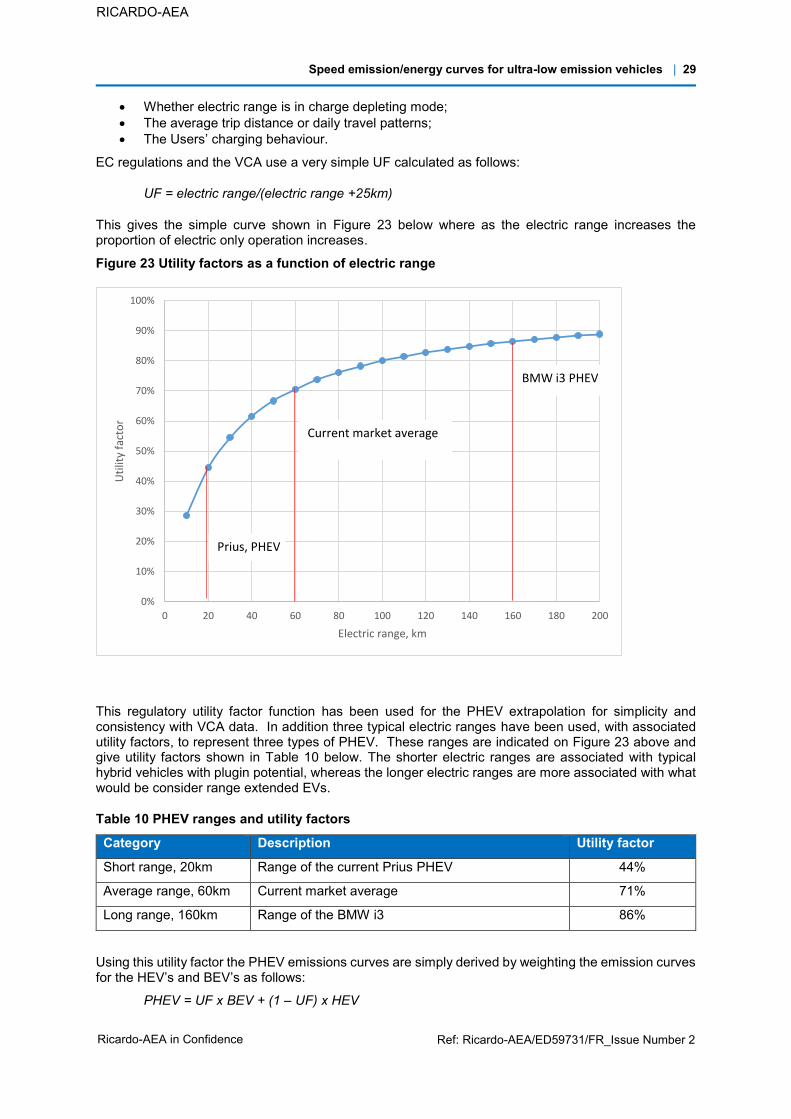
This gives the simple curve shown in Figure 23 below where as the electric range increases the proportion of electric only operation increases.
Figure 23 Utility factors as a function of electric range
This regulatory utility factor function has been used for the PHEV extrapolation for simplicity and consistency with VCA data. In addition three typical electric ranges have been used, with associated utility factors, to represent three types of PHEV. These ranges are indicated on Figure 23 above and give utility factors shown in Table 10 below. The shorter electric ranges are associated with typical hybrid vehicles with plugin potential, whereas the longer electric ranges are more associated with what would be consider range extended EVs.
Table 10 PHEV ranges and utility factors Category Description Utility factor
Short range, 20km Range of the current Prius PHEV 44%
Average range, 60km Current market average 71%
Long range, 160km Range of the BMW i3 86%
Using this utility factor the PHEV emissions curves are simply derived by weighting the emission curves for the HEV’s and BEV’s as follows:
PHEV = UF x BEV + (1 – UF) x HEV
0%
10%
20%
30%
40%
50%
60%
70%
80%
90%
100%
0 20 40 60 80 100 120 140 160 180 200
Uti
lity
fact
or
Electric range, km
Prius, PHEV
BMW i3 PHEV
Current market average
Speed emission/energy curves for ultra-low emission vehicles | 30
Ricardo-AEA in Confidence Ref: Ricardo-AEA/ED59731/FR_Issue Number 2
RICARDO-AEA
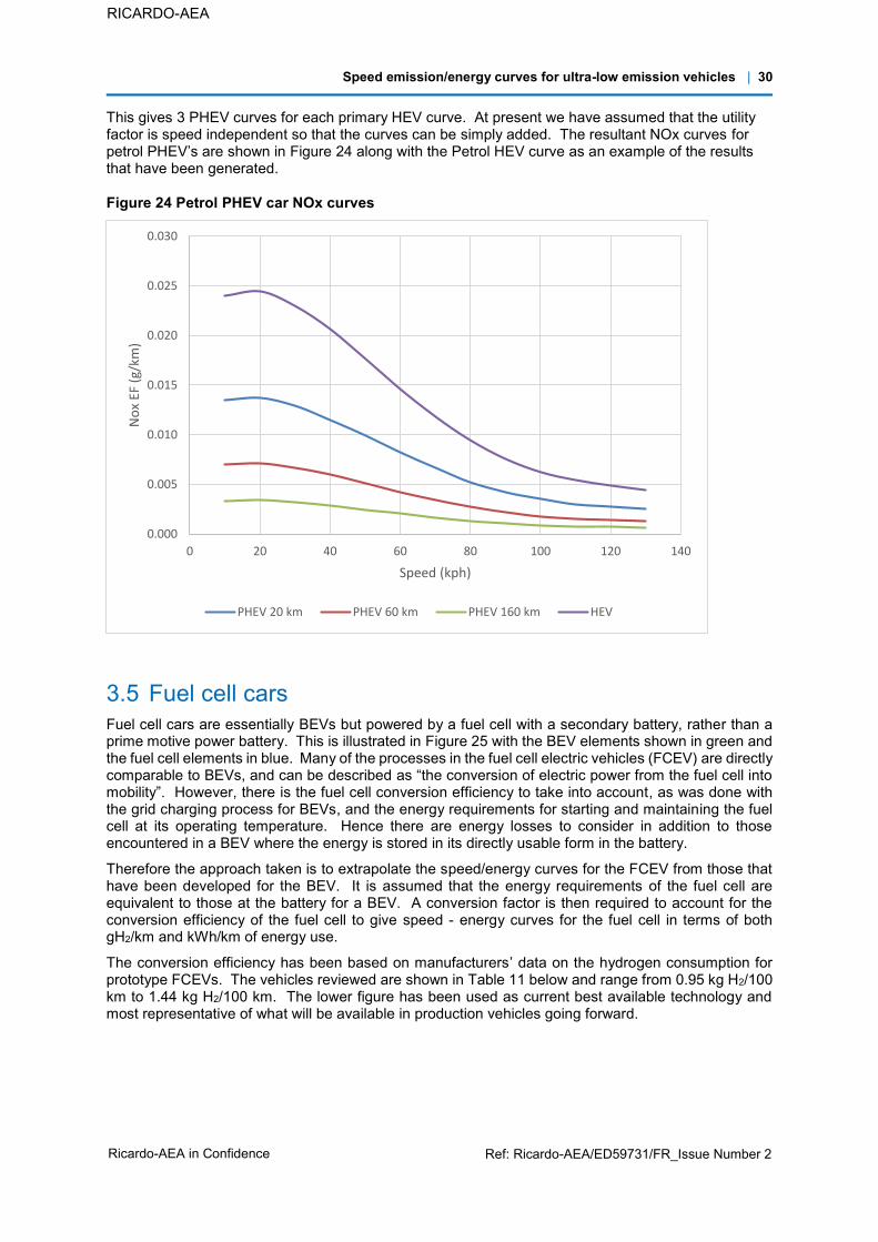
This gives 3 PHEV curves for each primary HEV curve. At present we have assumed that the utility factor is speed independent so that the curves can be simply added. The resultant NOx curves for petrol PHEV’s are shown in Figure 24 along with the Petrol HEV curve as an example of the results that have been generated.
Figure 24 Petrol PHEV car NOx curves
3.5 Fuel cell cars Fuel cell cars are essentially BEVs but powered by a fuel cell with a secondary battery, rather than a prime motive power battery. This is illustrated in Figure 25 with the BEV elements shown in green and the fuel cell elements in blue. Many of the processes in the fuel cell electric vehicles (FCEV) are directly comparable to BEVs, and can be described as “the conversion of electric power from the fuel cell into mobility”. However, there is the fuel cell conversion efficiency to take into account, as was done with the grid charging process for BEVs, and the energy requirements for starting and maintaining the fuel cell at its operating temperature. Hence there are energy losses to consider in addition to those encountered in a BEV where the energy is stored in its directly usable form in the battery.
Therefore the approach taken is to extrapolate the speed/energy curves for the FCEV from those that have been developed for the BEV. It is assumed that the energy requirements of the fuel cell are equivalent to those at the battery for a BEV. A conversion factor is then required to account for the conversion efficiency of the fuel cell to give speed - energy curves for the fuel cell in terms of both gH2/km and kWh/km of energy use.
The conversion efficiency has been based on manufacturers’ data on the hydrogen consumption for prototype FCEVs. The vehicles reviewed are shown in Table 11 below and range from 0.95 kg H2/100 km to 1.44 kg H2/100 km. The lower figure has been used as current best available technology and most representative of what will be available in production vehicles going forward.
0.000
0.005
0.010
0.015
0.020
0.025
0.030
0 20 40 60 80 100 120 140
No
x EF
(g/
km)
Speed (kph)
PHEV 20 km PHEV 60 km PHEV 160 km HEV

Speed emission/energy curves for ultra-low emission vehicles | 31
Ricardo-AEA in Confidence Ref: Ricardo-AEA/ED59731/FR_Issue Number 2
RICARDO-AEA
Figure 25 Energy processes in an FCEV
The mass of the Hyundai FCEV is 1,850kg, so assuming the motive energy consumption is the same as a BEV using the relationship in Figure 21 the energy required at the battery/fuel cell (FC) would be 17.1 kWh/100km. On this basis 55.63 g H2 in a FC passenger car is equivalent to 1 kWh in an analogous BEV for the battery – wheels energy consumption.
Table 11 Manufacturers’ data for FCEV fuel consumption
Vehicle kerb weight, kg quoted fuel consumption kg H2/100 km
Honda Clarity 1,628 60 mi/kg H2 1.04
Toyota and GM demonstrator vehicle based on the Chevrolet Equinox 2,010 320 km on 4.2 kg H2 1.32
Hyundai iX35-FC 1,850 594 km on 5.64 kg H2 0.95
Intelligent Energy/Lotus black cab FC – showcased at the Olympics 2,180 257 km on 3.7 kg H2 1.44
The BEV speed curves for passenger cars and vans have been defined as the mains plug – wheels energy consumption. This is taken as 100/88 of the battery – wheels energy consumption to account for the conversion efficiency from mains to battery. Therefore the 55.63 g H2 in a FC passenger car is equivalent to 1.136 kWh mains plug – wheels energy consumption, i.e. 48.95 g H2 in a FC passenger car are equivalent to 1.00 kWh mains socket – wheels energy consumption for a battery electric vehicle.
Therefore the FCEV curves have been generated by applying the scaling factor of 48.95 to the BEV results to provide results in terms of gH2/km. A single FCEV car has been generated based on a vehicle mass of 1,850 kg. Therefore the BEV car curve for a medium BEV of mass 1,500kg has been scaled using the mass-energy use relationship in Figure 21 to provide the energy requirements in terms of kWh/km and then scaled with the H2 factor to give fuel consumption in g H2/km.
3.6 HEV vans 3.6.1 Petrol The number of petrol vans of any type is fairly limited and they are all essentially car derived vans. Therefore given the lack of any other data we have simply assumed that the petrol HEV vans are the same as petrol HEV cars. They will have the same NOx and PM curve as the car curves and will have a single CO2/energy use curve taken from the medium sized petrol HEV car CO2/energy curve.

Speed emission/energy curves for ultra-low emission vehicles | 32
Ricardo-AEA in Confidence Ref: Ricardo-AEA/ED59731/FR_Issue Number 2
RICARDO-AEA
Since no petrol HEV vans currently exist only a Euro 6 version will be included as a likely future vehicle.
3.6.2 Diesel The majority of vans are diesel and there is a much wider range of sizes that are grouped into three classes for legislative purposes:
Class 1: Reference Mass < 1,305kg Class 2: Reference Mass 1,305kg to 1,760kg Class 3: Reference Mass 1,760kg
It would be possible to extrapolate the diesel HEV vans from the diesel HEV car curves. However, since the data on the diesel HEV cars is more limited than for petrol cars and the current curve has been generated from data on a single vehicle, it was felt prudent to also look at other potential sources of data rather than simply extrapolate from curves developed for cars.
To date there are no OEM diesel hybrid vans, only retrofit conversions such as the Connaught system which are not full hybrids. However, there are a number of hybrid trucks available which can provide useful data. Two key studies were available from the NREL in the US for a UPS hybrid truck and a Coca-Cola truck (NREL, 2013b and NREL, 2012). The data from these studies have been used to interpolate curves for diesel HEV vans as described below.
CO2 and fuel consumption curves
Both of the studies showed similar patterns of CO2 emissions reduction against a standard diesel vehicle in relation to speed. They showed significant reductions at lower speeds but little at higher speeds. The data in terms of CO2 reductions from the UPS HEV truck is shown in Table 12.
Table 12 Speed-CO2 relation for UPS hybrid truck Speed mph Speed kph CO2 reduction
5 8 32%
10 16 31%
22 35 25%
28 45 13%
30 48 6%
31.25 50 0%
These data have been used to generate a speed-CO2 reduction curve for a diesel HEV van relative to a standard diesel ICE as shown in Figure 26. This curve has been used to scale the existing diesel ICE CO2 curves to provide CO2 curves for the diesel HEV vans. An example of the resultant curve for a class 3 van is shown in Figure 27. The curve derived directly from applying the CO2 reduction curve is shown in green and shows a discontinuity at 50 kph. To remove this, the scaled data were re-fit to a new, smooth curve shown in black.

Speed emission/energy curves for ultra-low emission vehicles | 33
Ricardo-AEA in Confidence Ref: Ricardo-AEA/ED59731/FR_Issue Number 2
RICARDO-AEA
Figure 26 Diesel HEV van speed-CO2 emissions reduction curve
Figure 27 Speed-CO2 curve for a class 3 diesel HEV van
NOx and PM emission curves The emissions test data from the NREL report was measured using three different urban test cycles. Each had a similar average speed between 20kph and 25kph. However the change in NOx emissions of the hybrid versus the standard ICE was quite different showing increases in NOx of 30%, 15% and 0% for the three different cycles, and an average increase of around 15% (but with a high uncertainty). So like the diesel HEV car emission results the data are variable and difficult to draw conclusions from. However, like the diesel HEV car emission results the data do indicate that NOx emissions increase for diesel hybrid vehicles relative to their diesel ICE counterparts, and that CO2 emissions decrease, although the data do not provide a clear speed dependence.
0%
5%
10%
15%
20%
25%
30%
35%
0 10 20 30 40 50 60
CO
2 re
duct
ion
for h
ybrid
rela
tive
to
conv
entio
nal p
ower
train
Speed (kph)

Speed emission/energy curves for ultra-low emission vehicles | 34
Ricardo-AEA in Confidence Ref: Ricardo-AEA/ED59731/FR_Issue Number 2
RICARDO-AEA
For the three urban test cycles used in the NREL research study average speeds were around 20 kph, with negligible time spent above 40 kph. It therefore appears that the speeds where the NOx emissions increase and the CO2 emissions decrease both occur in this low speed range. This differs from the single diesel HEV car NOx emissions data where the NOx penalty appears to occur at speeds above 40 kph.
Because there are only limited data a simplified approach has been taken to derive an estimated NOx emission curve for diesel HEV vans. The evidence suggests that there is a NOx penalty of around 15% at urban speeds8. However, there are insufficient data to indicate the shape of the speed-NOx emission curve. Therefore the curve was generated by assigning the 15% additional impact to the shape of the speed-CO2 emissions reduction curve (where there is a 30% reduction over the same speed range)9. An example of the generated curve for a class 1 LGV is shown in Figure 28.
Figure 28 Derived NOx curve for a Class 1 diesel HEV van
These curves are based on evidence from trends in hybrid trucks in the U.S. The approach is consistent with the trend apparent for diesel HEV cars relative to their ICE counterpart, although it leads to a conclusion that for vans, the NOx penalty, that is where emissions for the HEV are higher than for an ICE, occurs at a lower speed.
At present, there are no data of any description (including manufacturers) to verify the curves. In the short term, the number of diesel hybrid vans is likely to be very small and one would anticipate that if and when the numbers grow, so some measurements of emissions will start to become available even if only from manufacturers and if only to support the directional change in emissions relative to an ICE van.
For PM, the very low emission factors adopted by TRL and used for conventional Euro 6 diesel vans are assumed for diesel HEV vans, the same assumption applied to diesel HEV cars.
8 The data in Table 12 and in Figure 26 indicate that around an average speed of 20 kph there is a reduction in CO2 emissions of around 30%. At around the same speed there is an average increase in NOx emissions of around 15% (albeit with high uncertainty). 9 This evidence indicates relative to a diesel ICE van the NOx emissions are half the magnitude of, and opposite in direction to, the change shown by CO2 (i.e. there is -50% scaling factor). This scaling function is then applied to the current COPERT ICE diesel van NOx curves to provide comparative NOx curves for diesel HEV van.
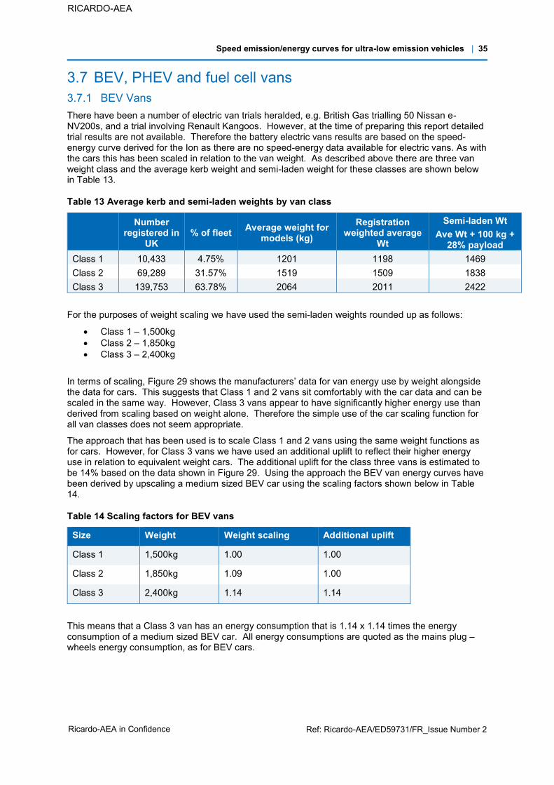
Speed emission/energy curves for ultra-low emission vehicles | 35
Ricardo-AEA in Confidence Ref: Ricardo-AEA/ED59731/FR_Issue Number 2
RICARDO-AEA
3.7 BEV, PHEV and fuel cell vans 3.7.1 BEV Vans There have been a number of electric van trials heralded, e.g. British Gas trialling 50 Nissan e-NV200s, and a trial involving Renault Kangoos. However, at the time of preparing this report detailed trial results are not available. Therefore the battery electric vans results are based on the speed-energy curve derived for the Ion as there are no speed-energy data available for electric vans. As with the cars this has been scaled in relation to the van weight. As described above there are three van weight class and the average kerb weight and semi-laden weight for these classes are shown below in Table 13.
Table 13 Average kerb and semi-laden weights by van class
Number
registered in UK
% of fleet Average weight for models (kg)
Registration weighted average
Wt
Semi-laden Wt Ave Wt + 100 kg +
28% payload Class 1 10,433 4.75% 1201 1198 1469 Class 2 69,289 31.57% 1519 1509 1838 Class 3 139,753 63.78% 2064 2011 2422
For the purposes of weight scaling we have used the semi-laden weights rounded up as follows:
Class 1 – 1,500kg Class 2 – 1,850kg Class 3 – 2,400kg
In terms of scaling, Figure 29 shows the manufacturers’ data for van energy use by weight alongside the data for cars. This suggests that Class 1 and 2 vans sit comfortably with the car data and can be scaled in the same way. However, Class 3 vans appear to have significantly higher energy use than derived from scaling based on weight alone. Therefore the simple use of the car scaling function for all van classes does not seem appropriate.
The approach that has been used is to scale Class 1 and 2 vans using the same weight functions as for cars. However, for Class 3 vans we have used an additional uplift to reflect their higher energy use in relation to equivalent weight cars. The additional uplift for the class three vans is estimated to be 14% based on the data shown in Figure 29. Using the approach the BEV van energy curves have been derived by upscaling a medium sized BEV car using the scaling factors shown below in Table 14.
Table 14 Scaling factors for BEV vans
Size Weight Weight scaling Additional uplift
Class 1 1,500kg 1.00 1.00
Class 2 1,850kg 1.09 1.00
Class 3 2,400kg 1.14 1.14
This means that a Class 3 van has an energy consumption that is 1.14 x 1.14 times the energy consumption of a medium sized BEV car. All energy consumptions are quoted as the mains plug – wheels energy consumption, as for BEV cars.

Speed emission/energy curves for ultra-low emission vehicles | 36
Ricardo-AEA in Confidence Ref: Ricardo-AEA/ED59731/FR_Issue Number 2
RICARDO-AEA
Figure 29 Manufacturers’ energy use data for cars and vans
3.7.2 Plug-in HEV vans The plug-in HEV vans have been treated in the same way as plug-in HEV cars by combining the HEV and BEV curves through the use of a utility factor. Since PHEV vans are yet to be developed we have kept the approach simple. A single utility factor has been used based on the average electric range category for PHEV cars of 60 km, which gives the utility factor of 71% electric operation.
This utility factor has then been used to combine the HEV and BEV van data to give a single PHEV curve for petrol vans and 3 PHEV curves for diesel vans (1 for each class).
3.7.3 Fuel cell vans The approach taken for the fuel cell vans is exactly the same as for fuel cell cars. The BEV van curves are used as the basis and then scaled by the fuel efficiency scaling factor of 48.95 g hydrogen being equivalent to 1 kWh for a BEV, to provide curves for hydrogen fuel consumption in g H2/km.

Speed emission/energy curves for ultra-low emission vehicles | 37
Ricardo-AEA in Confidence Ref: Ricardo-AEA/ED59731/FR_Issue Number 2
RICARDO-AEA
4 Emission curves for HGVs The detailed analysis and results for each of the HGV technologies is set out in the sections below covering:
Dedicated methane HGVs Dual fuel diesel/methane HGVs BEV HGVs
4.1 Dedicated methane fuelled vehicles Curves have been derived for both rigid and articulated dedicated methane fuelled trucks, i.e. those running from a spark ignition (SI) gas engine. Existing emissions data for this technology are based on a literature review, primarily a study done by Ricardo-AEA (2013), and provide simple non-speed dependant factors. Some new data from an ongoing project has been used to generate a speed-depend curve for a rigid HGV. This has been scaled to provide curves for the different rigid and articulated HGV sizes and has been adjusted to ensure consistency with the existing non-speed dependant factors. The details of the approach are provided below.
4.1.1 Rigid HGVs NOx emissions
The Ricardo-AEA (2013) review carried out for Defra derived emissions factors for a dedicated methane fuelled 16t GVW rigid truck travelling at an average speed of 40 kph as follows:
NOx emissions PM emissions
For pre Euro VI vehicles with three way catalyst 1.6 g/km 0.007 g/km
For Euro VI vehicles with three way catalyst 0.5 g/km 0.01 g/km
It was noted that while the emission factors for the three-way catalyst (TWC) (pre-Euro VI) vehicles in this table were based on the evidence gathered from literature and through consultations, there were no equivalent data for Euro VI methane fuelled vehicles. Therefore the emissions factors for Euro VI vehicles were based on the changes in emissions required for Euro V vehicles to meet the Euro VI standards. The more recent evidence reviewed in this study has identified no contradictory data to these basic factors.
However, it is also noted that the evidence available was predominantly collected for methane fuelled buses. These weigh typically around 15 tonnes, and the emissions were actually measured over cycles whose average speed was around 20 kph. The data were extrapolated to 40 kph using changes in engine power required to drive at the different average speed, and the assumption that NOx emissions are proportional to power.
As noted the data available in the literature were not speed dependent emissions. Furthermore, the difference in combustion chemistry between diesel compression ignition (CI) and methane spark ignition (SI) vehicles means that scaling a speed NOx curve from a diesel engine to provide the shape for the speed NOx curve from a SI engined vehicle is not appropriate. For example comparison of the COPERT speed NOx emission curves for diesel and petrol fuelled Class 3 light commercial vehicles shows they are clearly different.
Therefore some direct speed related NOx data was needed and this was available in the form of NOx emissions data collected during the DfT Methane Slip protocol project. The modal data from four repeats, measured for a dedicated methane fuelled 26 tonne rigid truck, over the World Harmonised Vehicle Cycle were analysed, allocating each second’s data into a speed window that was 2.5 kph wide. Figure 30 below shows these data, with the different coloured circles representing the four runs. The orange line shows the polynomial fitted through the data.
When this overall shape is compared with that in COPERT 4 for the speed NOx emission curves for petrol fuelled vans it can be seen that they are broadly of a similar shape, but distinctly different to the speed NOx emission curves for diesel comparator vans.

Speed emission/energy curves for ultra-low emission vehicles | 38
Ricardo-AEA in Confidence Ref: Ricardo-AEA/ED59731/FR_Issue Number 2
RICARDO-AEA
Figure 30 Speed-NOx emission data for a dedicated methane 26t HGV
The speed-emissions data collected within the DfT Methane slip protocol project is for a 26 tonne rigid truck, therefore to compare with the existing data the emissions factors for a 16 tonne truck as reported in Ricardo-AEA (2013) were extrapolated to provide an estimate for 26 tonne rigid HGV. This original evidence, suggested the NOx emissions for a 26 tonne truck would be around 3.2 g/km for pre Euro VI vehicles with TWC at 20 kph, and 1.00 for Euro VI vehicles with TWC at 20 kph.
The function fitted to the DfT Methane slip data indicates NOx emissions of 3.86 at 20 kph, compared to 3.2 g/km for a 26 tonne truck estimated above. Therefore to generate a general speed-NOx curve for a 26 tonne rigid truck consistent with the existing data the curve above was multiplied by 0.83 for pre-Euro VI vehicles and 0.26 for Euro VI vehicles, to give NOx emissions of 3.2 g/km and 1.0 g/km, respectively, at 20 kph.
CO2 emissions
The differences in combustion conditions for an ICE means that a CO2 curve for a dedicated gas-fuelled SI HGV cannot be inferred from diesel engine vehicles. Therefore the CO2 emissions data collected during the DfT Methane Slip protocol project were similarly analysed and fitted. This is shown in Figure 31.
In comparison with this a study by CENEX comparing the performance of a dedicated methane truck and a diesel comparator, noted that over the Coca-Cola Enterprises real world cycle the methane vehicle had 8.7% higher tailpipe CO2 emissions. Interestingly, the diesel comparator CO2 emissions measured in the CENEX study of 843 g/km are identical to those in the DfT CO2 emissions factors database for a 26 – 28 tonne Euro V rigid truck at 40 kph.
Although the CENEX study did not provide speed related data it provided good indication of the relative difference between the CO2 emissions for a methane truck over a diesel truck. Therefore for the speed-emission curves derived in this project, the shape of a speed-CO2 curve for this 26 tonne rigid truck from the methane slip project was retained and this was scaled to the CO2 emissions at 40 kph found in the Cenex study, i.e. 8.7% higher than the comparator diesel vehicle.
The same function was assumed to apply for both pre-Euro VI and Euro VI 26 tonne rigid trucks.
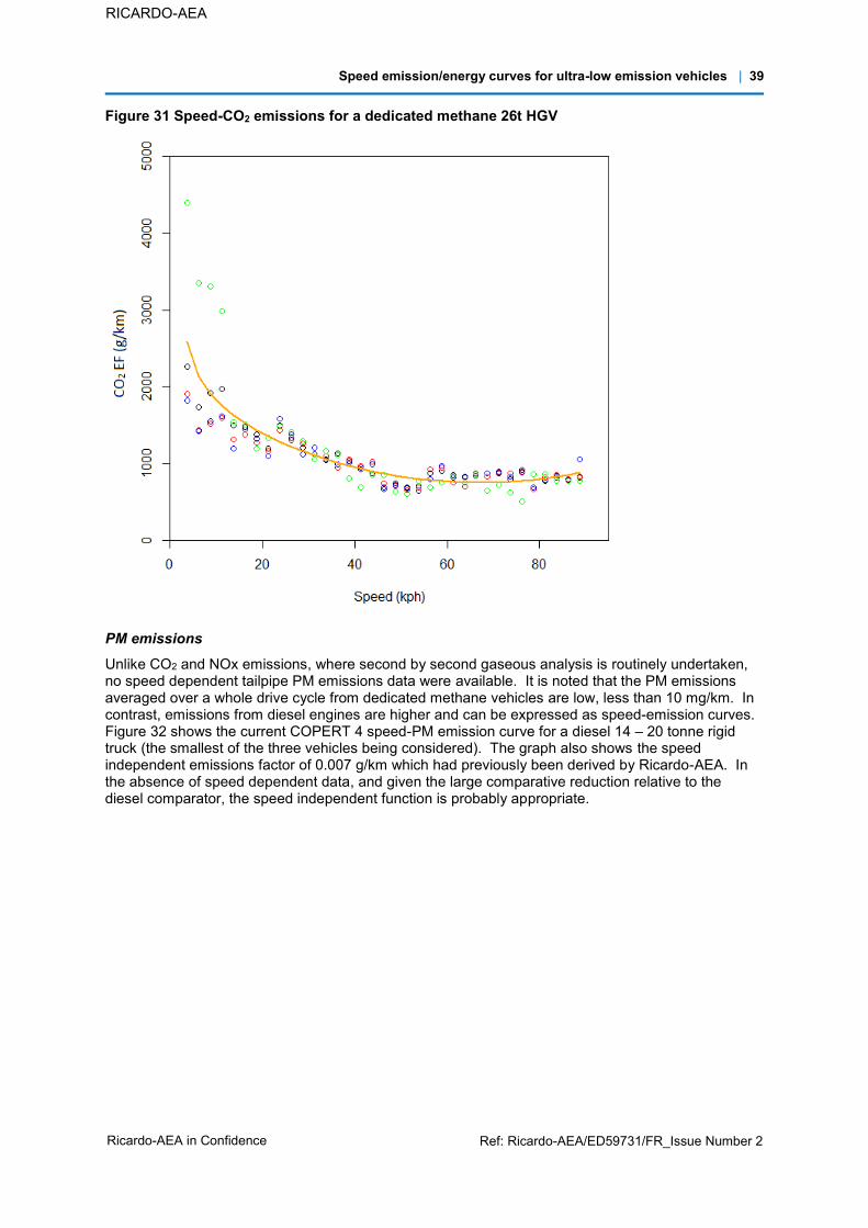
Speed emission/energy curves for ultra-low emission vehicles | 39
Ricardo-AEA in Confidence Ref: Ricardo-AEA/ED59731/FR_Issue Number 2
RICARDO-AEA
Figure 31 Speed-CO2 emissions for a dedicated methane 26t HGV
PM emissions
Unlike CO2 and NOx emissions, where second by second gaseous analysis is routinely undertaken, no speed dependent tailpipe PM emissions data were available. It is noted that the PM emissions averaged over a whole drive cycle from dedicated methane vehicles are low, less than 10 mg/km. In contrast, emissions from diesel engines are higher and can be expressed as speed-emission curves. Figure 32 shows the current COPERT 4 speed-PM emission curve for a diesel 14 – 20 tonne rigid truck (the smallest of the three vehicles being considered). The graph also shows the speed independent emissions factor of 0.007 g/km which had previously been derived by Ricardo-AEA. In the absence of speed dependent data, and given the large comparative reduction relative to the diesel comparator, the speed independent function is probably appropriate.
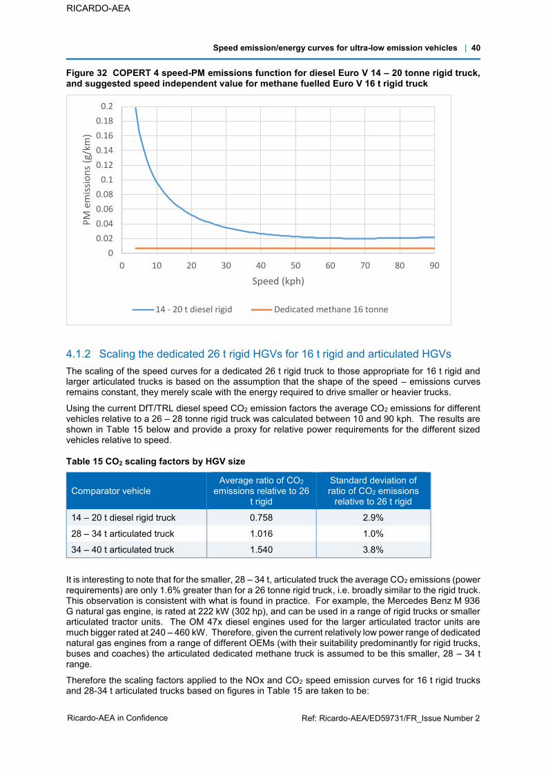
Speed emission/energy curves for ultra-low emission vehicles | 40
Ricardo-AEA in Confidence Ref: Ricardo-AEA/ED59731/FR_Issue Number 2
RICARDO-AEA
Figure 32 COPERT 4 speed-PM emissions function for diesel Euro V 14 – 20 tonne rigid truck, and suggested speed independent value for methane fuelled Euro V 16 t rigid truck
4.1.2 Scaling the dedicated 26 t rigid HGVs for 16 t rigid and articulated HGVs The scaling of the speed curves for a dedicated 26 t rigid truck to those appropriate for 16 t rigid and larger articulated trucks is based on the assumption that the shape of the speed – emissions curves remains constant, they merely scale with the energy required to drive smaller or heavier trucks.
Using the current DfT/TRL diesel speed CO2 emission factors the average CO2 emissions for different vehicles relative to a 26 – 28 tonne rigid truck was calculated between 10 and 90 kph. The results are shown in Table 15 below and provide a proxy for relative power requirements for the different sized vehicles relative to speed.
Table 15 CO2 scaling factors by HGV size
Comparator vehicle Average ratio of CO2
emissions relative to 26 t rigid
Standard deviation of ratio of CO2 emissions
relative to 26 t rigid
14 – 20 t diesel rigid truck 0.758 2.9%
28 – 34 t articulated truck 1.016 1.0%
34 – 40 t articulated truck 1.540 3.8%
It is interesting to note that for the smaller, 28 – 34 t, articulated truck the average CO2 emissions (power requirements) are only 1.6% greater than for a 26 tonne rigid truck, i.e. broadly similar to the rigid truck. This observation is consistent with what is found in practice. For example, the Mercedes Benz M 936 G natural gas engine, is rated at 222 kW (302 hp), and can be used in a range of rigid trucks or smaller articulated tractor units. The OM 47x diesel engines used for the larger articulated tractor units are much bigger rated at 240 – 460 kW. Therefore, given the current relatively low power range of dedicated natural gas engines from a range of different OEMs (with their suitability predominantly for rigid trucks, buses and coaches) the articulated dedicated methane truck is assumed to be this smaller, 28 – 34 t range.
Therefore the scaling factors applied to the NOx and CO2 speed emission curves for 16 t rigid trucks and 28-34 t articulated trucks based on figures in Table 15 are taken to be:
0
0.02
0.04
0.06
0.08
0.1
0.12
0.14
0.16
0.18
0.2
0 10 20 30 40 50 60 70 80 90
PM
em
issi
on
s (g
/km
)
Speed (kph)
14 - 20 t diesel rigid Dedicated methane 16 tonne
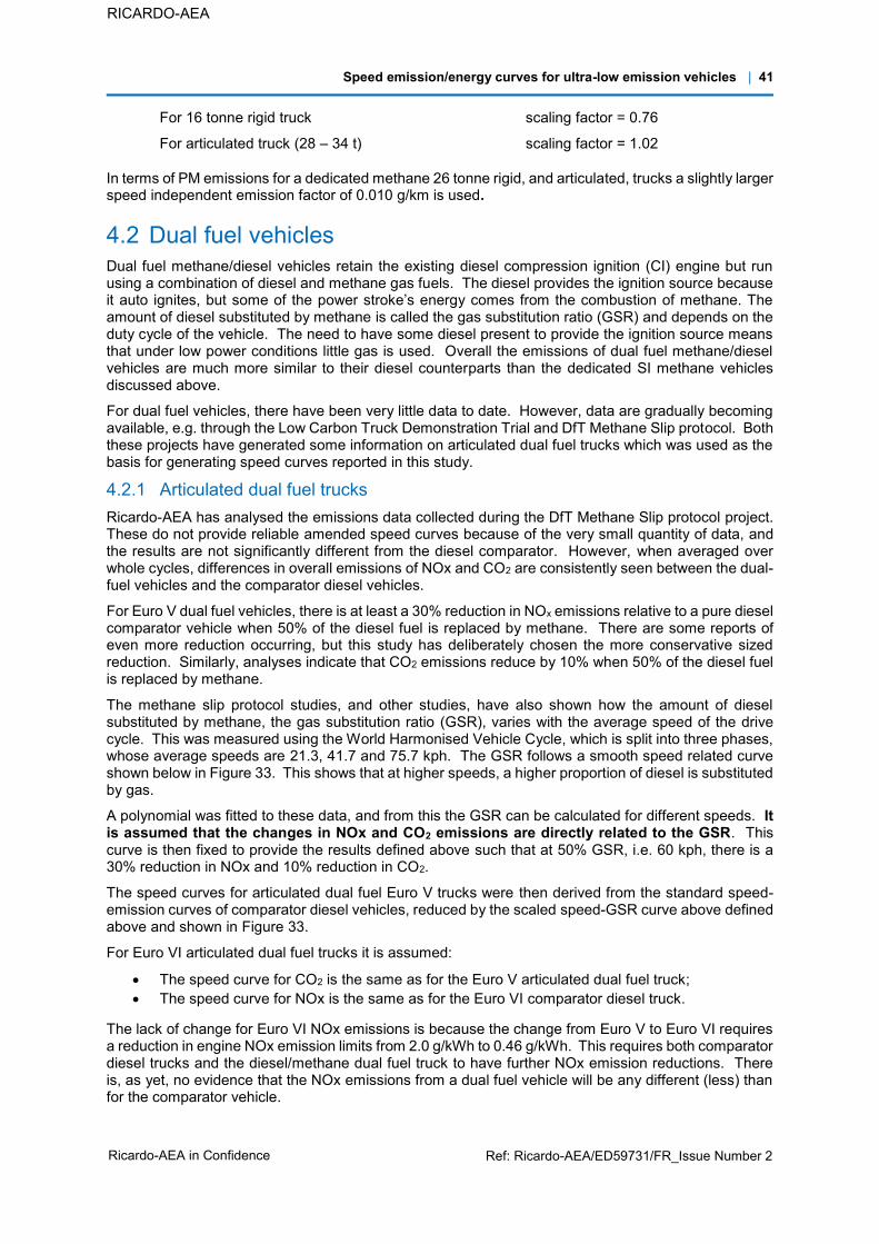
Speed emission/energy curves for ultra-low emission vehicles | 41
Ricardo-AEA in Confidence Ref: Ricardo-AEA/ED59731/FR_Issue Number 2
RICARDO-AEA
For 16 tonne rigid truck scaling factor = 0.76
For articulated truck (28 – 34 t) scaling factor = 1.02
In terms of PM emissions for a dedicated methane 26 tonne rigid, and articulated, trucks a slightly larger speed independent emission factor of 0.010 g/km is used.
4.2 Dual fuel vehicles Dual fuel methane/diesel vehicles retain the existing diesel compression ignition (CI) engine but run using a combination of diesel and methane gas fuels. The diesel provides the ignition source because it auto ignites, but some of the power stroke’s energy comes from the combustion of methane. The amount of diesel substituted by methane is called the gas substitution ratio (GSR) and depends on the duty cycle of the vehicle. The need to have some diesel present to provide the ignition source means that under low power conditions little gas is used. Overall the emissions of dual fuel methane/diesel vehicles are much more similar to their diesel counterparts than the dedicated SI methane vehicles discussed above.
For dual fuel vehicles, there have been very little data to date. However, data are gradually becoming available, e.g. through the Low Carbon Truck Demonstration Trial and DfT Methane Slip protocol. Both these projects have generated some information on articulated dual fuel trucks which was used as the basis for generating speed curves reported in this study.
4.2.1 Articulated dual fuel trucks Ricardo-AEA has analysed the emissions data collected during the DfT Methane Slip protocol project. These do not provide reliable amended speed curves because of the very small quantity of data, and the results are not significantly different from the diesel comparator. However, when averaged over whole cycles, differences in overall emissions of NOx and CO2 are consistently seen between the dual-fuel vehicles and the comparator diesel vehicles.
For Euro V dual fuel vehicles, there is at least a 30% reduction in NOx emissions relative to a pure diesel comparator vehicle when 50% of the diesel fuel is replaced by methane. There are some reports of even more reduction occurring, but this study has deliberately chosen the more conservative sized reduction. Similarly, analyses indicate that CO2 emissions reduce by 10% when 50% of the diesel fuel is replaced by methane.
The methane slip protocol studies, and other studies, have also shown how the amount of diesel substituted by methane, the gas substitution ratio (GSR), varies with the average speed of the drive cycle. This was measured using the World Harmonised Vehicle Cycle, which is split into three phases, whose average speeds are 21.3, 41.7 and 75.7 kph. The GSR follows a smooth speed related curve shown below in Figure 33. This shows that at higher speeds, a higher proportion of diesel is substituted by gas.
A polynomial was fitted to these data, and from this the GSR can be calculated for different speeds. It is assumed that the changes in NOx and CO2 emissions are directly related to the GSR. This curve is then fixed to provide the results defined above such that at 50% GSR, i.e. 60 kph, there is a 30% reduction in NOx and 10% reduction in CO2.
The speed curves for articulated dual fuel Euro V trucks were then derived from the standard speed-emission curves of comparator diesel vehicles, reduced by the scaled speed-GSR curve above defined above and shown in Figure 33.
For Euro VI articulated dual fuel trucks it is assumed:
The speed curve for CO2 is the same as for the Euro V articulated dual fuel truck; The speed curve for NOx is the same as for the Euro VI comparator diesel truck.
The lack of change for Euro VI NOx emissions is because the change from Euro V to Euro VI requires a reduction in engine NOx emission limits from 2.0 g/kWh to 0.46 g/kWh. This requires both comparator diesel trucks and the diesel/methane dual fuel truck to have further NOx emission reductions. There is, as yet, no evidence that the NOx emissions from a dual fuel vehicle will be any different (less) than for the comparator vehicle.
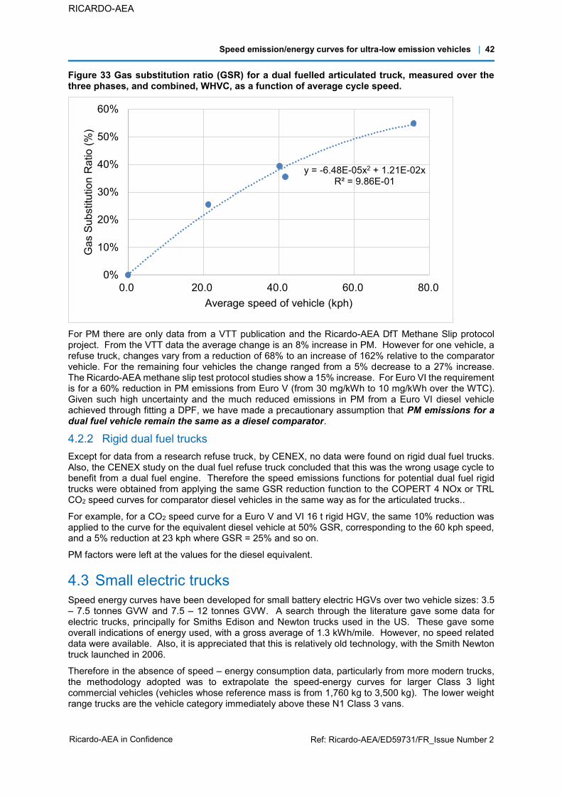
Speed emission/energy curves for ultra-low emission vehicles | 42
Ricardo-AEA in Confidence Ref: Ricardo-AEA/ED59731/FR_Issue Number 2
RICARDO-AEA
Figure 33 Gas substitution ratio (GSR) for a dual fuelled articulated truck, measured over the three phases, and combined, WHVC, as a function of average cycle speed.
For PM there are only data from a VTT publication and the Ricardo-AEA DfT Methane Slip protocol project. From the VTT data the average change is an 8% increase in PM. However for one vehicle, a refuse truck, changes vary from a reduction of 68% to an increase of 162% relative to the comparator vehicle. For the remaining four vehicles the change ranged from a 5% decrease to a 27% increase. The Ricardo-AEA methane slip test protocol studies show a 15% increase. For Euro VI the requirement is for a 60% reduction in PM emissions from Euro V (from 30 mg/kWh to 10 mg/kWh over the WTC). Given such high uncertainty and the much reduced emissions in PM from a Euro VI diesel vehicle achieved through fitting a DPF, we have made a precautionary assumption that PM emissions for a dual fuel vehicle remain the same as a diesel comparator.
4.2.2 Rigid dual fuel trucks Except for data from a research refuse truck, by CENEX, no data were found on rigid dual fuel trucks. Also, the CENEX study on the dual fuel refuse truck concluded that this was the wrong usage cycle to benefit from a dual fuel engine. Therefore the speed emissions functions for potential dual fuel rigid trucks were obtained from applying the same GSR reduction function to the COPERT 4 NOx or TRL CO2 speed curves for comparator diesel vehicles in the same way as for the articulated trucks..
For example, for a CO2 speed curve for a Euro V and VI 16 t rigid HGV, the same 10% reduction was applied to the curve for the equivalent diesel vehicle at 50% GSR, corresponding to the 60 kph speed, and a 5% reduction at 23 kph where GSR = 25% and so on.
PM factors were left at the values for the diesel equivalent.
4.3 Small electric trucks Speed energy curves have been developed for small battery electric HGVs over two vehicle sizes: 3.5 – 7.5 tonnes GVW and 7.5 – 12 tonnes GVW. A search through the literature gave some data for electric trucks, principally for Smiths Edison and Newton trucks used in the US. These gave some overall indications of energy used, with a gross average of 1.3 kWh/mile. However, no speed related data were available. Also, it is appreciated that this is relatively old technology, with the Smith Newton truck launched in 2006.
Therefore in the absence of speed – energy consumption data, particularly from more modern trucks, the methodology adopted was to extrapolate the speed-energy curves for larger Class 3 light commercial vehicles (vehicles whose reference mass is from 1,760 kg to 3,500 kg). The lower weight range trucks are the vehicle category immediately above these N1 Class 3 vans.
y = -6.48E-05x2 + 1.21E-02xR² = 9.86E-01
0%
10%
20%
30%
40%
50%
60%
0.0 20.0 40.0 60.0 80.0
Gas
Sub
stitu
tion
Rat
io (%
)
Average speed of vehicle (kph)

Speed emission/energy curves for ultra-low emission vehicles | 43
Ricardo-AEA in Confidence Ref: Ricardo-AEA/ED59731/FR_Issue Number 2
RICARDO-AEA
The standard TRL speed – fuel consumption curves for these vehicles give their speed-energy requirements when fitted with diesel ICEs. These are shown in Figure 34 expressed as litres fuel consumed per 100 km travelled.
Figure 34 Fuel consumption of 3.5t to 12t rigids and a class 3 van
Using these data the ratio of fuel consumption for a 7.5-12 t HGV and a 3.5-7.5 t HGV relative to a N1 Class 3 van was calculated and is shown in Figure 35 below. From these figures it can be seen that the energy consumption for the 3.5 – 7.5 t rigid HGV is approximately a constant factor of 1.47 times higher than for the N1 Class 3 van. Therefore the smaller HGV will operate in a similar fashion to the Class 3 van, just using more energy because of its greater weight.
However, the energy consumption for the 7.5 – 12 t rigid HGVs is higher than the N1 Class 3 van by a ratio which is speed-dependent. Defined as an uplift, this ratio can be expressed as a linear function of speed:
Uplift (Speed) = 2.68 – 0.009 Speed
This gives an increase of 2.46 at 25 kph and 1.96 at 80 kph.
This then provides the speed-fuel consumption curves for these two sizes of trucks which can be used to define the speed dependence of the energy requirements of the electric HGVs relative to the curve already developed for the Class 3 van (which in itself is based on a BEV car).
At around 25 kph this model predicts an energy consumption for the larger truck of 0.59 kW/km, (0.95 kW /mile). This is considerably less than was found from a field trial of Smith Newton trucks (12 t GVW)10 which gives a range of energy consumptions from 0.62 to 1.00 kWh/km. It is presumed that some of this difference is caused by the relatively older technology of this vehicle compared with modern BEV cars and vans. It is also evident that these data support the on-the-road uplift for BEV discussed at the end of Section 3.3 that feed through into these speed-energy curves.
10 http://insideevs.com/smith-electric-vehicles-distance-energy-consumption/
0
5
10
15
20
25
30
35
40
45
0 20 40 60 80 100
Fuel
co
nsu
mp
tio
n (
l/1
00
km
)
Speed (km/h)
Fuel consumption (l/100 km) for different vehicles
N1 Class III 3.5 - 7.5 t rigid 7.5 - 12 t rigid
Speed emission/energy curves for ultra-low emission vehicles | 44
Ricardo-AEA in Confidence Ref: Ricardo-AEA/ED59731/FR_Issue Number 2
RICARDO-AEA
Figure 35 Fuel consumption for a 3.5-7.5t and a 7.5-12t rigid HGV relative to a N1 class 3 van
0.75
1
1.25
1.5
1.75
2
2.25
2.5
2.75
10 20 30 40 50 60 70 80 90
Rel
ativ
e fu
el c
onsu
mpt
ion
(rel t
o N
1 C
lass
3 v
an)
Speed (km/h)
Relative fuel consumption for different vehicles
N1 Class III
3.5 - 7.5 t rigid
7.5 - 12 t rigid
Linear (3.5 - 7.5 t rigid)
Linear (7.5 - 12 t rigid)
Speed emission/energy curves for ultra-low emission vehicles | 45
Ricardo-AEA in Confidence Ref: Ricardo-AEA/ED59731/FR_Issue Number 2
RICARDO-AEA
5 Aggregation tools
The previous sections describe the development of detailed emission curves for different ULEV categories. The vehicle categorisation was defined by the availability of test or modelled data, or by the means to make reasonable estimations and/or extrapolations. For use in the NTM it is necessary to aggregate the emission curves for variants within a main ULEV category, for example vehicles of different Euro classes, engine capacity ranges or vehicle weights.
A spreadsheet tool capable of performing this aggregation has been developed and provided to DfT. This tool adopts the same general approach taken by Ricardo-AEA in the development of the existing emission curves for conventional petrol and diesel vehicle types provided to DfT for the NTM in 2013. If the emission curves for all the variants are described by the same mathematical functional form, then an aggregate emission curve can be developed by weightings applied to each of the coefficients in the equations. The weightings are based on the fractions of each variant in the national fleet and are year-dependent. Coefficients which define the shape and magnitude of emissions curves for a given year are derived for each main vehicle type by summing the contributing weighted coefficients relevant to the year. The final result is a set of year-specific emission curves for each main class of ULEV and pollutant or fuel consumption combination.
The weightings used in the development of emission curves for conventional vehicles reflected the mix of vehicles meeting the different Euro classes in the fleet in a given year, from Euro 1/I to Euro 6/VI. These weighting were derived from the NAEI’s fleet turnover model which took account of historic and future new vehicle sales according to data provided by DfT, vehicle survival rates and data on mileage as a function of vehicle age. For the ULEVs investigated in this work, the weightings are somewhat simpler because all the vehicles will meet either Euro 5/V or 6/VI standards only (plus Euro 6c in the case of NOx curves for diesel cars and LGVs, although the emission curves for these have been left in the tool with the same value as for Euro 6 for the time being, for reasons explained in section 3.2). For some ULEVs, an important categorisation is made according to engine capacity or vehicle weight. However, ULEV technology is still in its infancy and current and future sales data remains under development and is likely to undergo regular updates as uptake of certain vehicle technologies are incentivised.
The aggregation spreadsheet tool provides flexibility to update curves as new information becomes available as it takes fleet composition data as an input. For this tool, it is left to DfT to provide the fleet weightings of the sub-categories (Euro standard, engine size or weight) of each ULEV category, but dummy fractions have been provided in the tool to demonstrate its functionality. The dummy fractions were also used as part of the QA/QC procedure, to test the aggregations are working correctly. Aggregation curves can be updated simply by inputting new fleet data into the tool.
The aggregation spreadsheet tool calculates aggregated emission curves for the three pollutants (CO2, NOx and PM), petrol and diesel fuel consumption and electricity and hydrogen consumption, as applicable for each ULEV category. Curves are output for years 2015, 2020, 2025, 2030, 2035 and 2040. The remainder of this section summarises the ULEV categories for which aggregate curves are output, the methodology for generating emission curves and the required classification of the weighting factors by main ULEV category.
5.1 ULEV categories After discussion with DfT it was agreed that emission curves for twenty-one ULEV categories would be provided within this project. The ULEV categories are summarised in Table 16 which also indicates which pollutant or fuel consumption types apply to each ULEV category. These main ULEV types encompass the range of vehicles discussed in Sections 3 and 4.
As part of the NTM, DfT further weight the curves for aggregated ULEV categories, plus curves for conventional vehicle types (e.g. petrol cars, diesel cars, buses etc.) by proportion of vehicle kilometres for the different vehicles by five area types (London, Conurbations, other urban, rural and motorways) to provide emissions for different road/area types. This additional aggregation step is not performed as part of this work.

Speed emission/energy curves for ultra-low emission vehicles | 46
Ricardo-AEA in Confidence Ref: Ricardo-AEA/ED59731/FR_Issue Number 2
RICARDO-AEA
Table 16 – Summary of ULEV category and pollutant/fuel consumption combinations for which aggregated speed-emission curves are provided.
Vehicle Aggregated vehicle type CO2 NOx PM Electricity
consumption Hydrogen
consumption
Car
Petrol Hybrid
Diesel Hybrid
Petrol Plugin 20 km
Petrol Plugin 60 km
Petrol Plugin 160 km
Diesel Plugin 20 km
Diesel Plugin 60 km
Diesel Plugin 160 km
Electric
Hydrogen
LGV
Petrol Hybrid
Diesel Hybrid
Petrol Plugin
Diesel Plugin
Electric
Hydrogen
Rigid HGV
Methane
Dual fuel
Electric
Artic HGV
Methane
Dual fuel
Section 3.4 discussed the dependence of speed-emission curves for plug-in cars on the electric range of the vehicle. Detailed emission factor curves were calculated for plug-in cars disaggregated not only by vehicle size and Euro standard but also by three electric ranges of 20, 60 and 160 km. There is evidence that the proportion of plug-in vehicles of different electric range is likely to be different in different area or road types. For example it maybe that plug-in vehicles with a longer electric range are likely to be more prevalent on motorways than urban roads as distances travelled are likely to be greater. Conversely a higher proportion of journeys on urban roads are likely to be accounted for by plug-in cars with a short electric range. It was agreed that three aggregated ULEV curves would be provided each for petrol and diesel plug-in cars for each of the three electric ranges. This will provide DfT with the capability to account for the different proportion of plug-in cars of different road types within the NTM.

Speed emission/energy curves for ultra-low emission vehicles | 47
Ricardo-AEA in Confidence Ref: Ricardo-AEA/ED59731/FR_Issue Number 2
RICARDO-AEA
5.2 Weighting factors by main ULEV class This section describes the curve weightings relevant to each main ULEV class and pollutant or fuel consumption combination. The Euro standard and vehicle size weighting factors themselves are not provided as part of this work, however the aggregation spreadsheet tool requires this information to be input. Year dependent Euro standard and vehicle size weighting factors should be provided for each main ULEV class for the years 2015, 2020, 2025, 2030, 2035 and 2040.
Table 17-19 summarise the Euro standard and vehicle size categories for which weighting factors are required to be split by within each ULEV class for cars, LGVs and HGVs. Note that the aggregation spreadsheet tool compiles aggregated EFs for different pollutant or fuel consumption types using the same Euro standard and vehicle size weighting factors, therefore the Euro standard and size categories in the tables are representative of the greatest degree of disaggregation of the detailed EF curves for a pollutant or fuel consumption type within a ULEV category. For example, the CO2 emission curves developed for Petrol HEV cars are split into three different size categories and two Euro standards (6 curves in total), while the NOx emission curve developed for this vehicle type is not dependent on vehicle size or Euro standard. The aggregation spreadsheet requires the Euro standard fleet weighting factors to be provided for two Euro standards and the fleet size weighting factors to be provided for three vehicle sizes to reflect the higher degree of disaggregation of the CO2 emission curves. Euro standard and vehicle size weighting factors must sum to 1 for each ULEV category.
Table 17: Euro standard and vehicle size categories for ULEV cars.
ULEV category Euro standard Sizes
Petrol HEV Euro 5 and 6 Small (<1.4 l), medium (1.4-2.0 l) and large (>2.0 l)
Diesel HEV Euro 5, 6 and 6c** Small (<1.4 l), medium (1.4-2.0 l) and large (>2.0 l)
BEV Euro 6 Small (<1300 kg), medium (1300-1850 kg) and large (>1850 kg)
Petrol PHEV 20 km Euro 6 Small, medium, large*
Petrol PHEV 60 km Euro 6 Small, medium, large*
Petrol PHEV 160 km Euro 6 Small, medium, large*
Diesel PHEV 20 km Euro 6 Small, medium, large*
Diesel PHEV 60 km Euro 6 Small, medium, large*
Diesel PHEV 160 km Euro 6 Small, medium, large*
Hydrogen Euro 6 One size
* For PHEVs small, medium and large are defined by the combination of small, medium and large HEVs and BEVs. ** At present, factors for Euro 6c are assumed to be the same as Euro 6 as they have not been included in the factors for conventional ICE diesel vehicles provided to DfT for the NTM in 2013/14. Including them for HEVs would make the curves not comparable with curves for diesel ICEs. A space for Euro 6c has been provided in the aggregation spreadsheet for inclusion at a later stage and we recommend this is done when the curves for diesel ICE cars are updated.

Speed emission/energy curves for ultra-low emission vehicles | 48
Ricardo-AEA in Confidence Ref: Ricardo-AEA/ED59731/FR_Issue Number 2
RICARDO-AEA
Table 18: Euro standard and vehicle size categories for ULEV LGVs.
ULEV category Euro standard Sizes
Petrol HEV Euro 5 and 6 One size
Diesel HEV Euro 5, 6 and 6c Class 1, 2 and 3
BEV Euro 6 Class 1, 2 and 3
Petrol PHEV Euro 6 Class 1, 2 and 3
Diesel PHEV Euro 6 Class 1, 2 and 3
Hydrogen Euro 6 Class 1, 2 and 3
Table 19: Euro standard and vehicle size categories for ULEV HGVs.
ULEV category Euro standard Sizes
Rigid Electric Euro VI 3.5-7.5 t and 7.5-12 t
Dedicated methane rigid Euro V and VI 14-20 t and 20-28 t
Dual fuel rigid Euro V and VI Single curve for all sizes weighted by mix of GVW classes in rigid fleet
Dedicated methane articulated Euro V and VI 34-50 t only
Dual fuel articulated Euro V and VI Single curve for all sizes weighted by mix of GVW classes in artic fleet
5.3 Generation of EF curves Emission factors for all the detailed vehicle categories were provided in the same mathematical functional form:
EF(v) = k (a + bv +cv2 + dv3 + ev4 + fv5 + gv6) / v (1)
Thus, it was straightforward to develop a single curve in the same form representing the average emission factor for all vehicles in the main ULEV category in a given year by weighting all the common coefficients according to the composition of the vehicle fleet in that year.
The aggregation spreadsheet tool provides a means to calculate emission curves for the main vehicle types. In summary, the emission curves developed take the 6th order polynomial form:
EFy(v) = (Ay + Byv +Cyv2 + Dyv3 + Eyv4 + Fyv5 + Gyv6) / v (2)
The seven coefficients A-G for the main vehicle types in each year are weightings of the individual coefficients for the different constituent Euro standards and vehicle or engine sizes which make up the fleet according to the fractions in the fleet in the year. This is expressed mathematically in Equation 3 which shows how the coefficient A is calculated for a particular main vehicle category in year y:
e wywyeewewy SRakA
(3)
Rye is the fraction of vkm by vehicles of Euro standard e in year y.
Syw is the fraction of vkm by vehicles of size or weight class w in year y.
kew and aew are the speed emission factor coefficients for vehicle of Euro standard e and size w within a main vehicle category.
Speed emission/energy curves for ultra-low emission vehicles | 49
Ricardo-AEA in Confidence Ref: Ricardo-AEA/ED59731/FR_Issue Number 2
RICARDO-AEA
Similar expressions can be derived for the other coefficients B-G by replacing the coefficient aew with the appropriate coefficient.
5.4 Further weighting and adjustment for HGV curves For both the dedicated methane and dual fuel HGVs, emission and fuel consumption curves were developed for specific weight classes of HGVs. This reflected the weight classes for which data were available. In the case of dedicated methane vehicles, the general consensus is that the 16t and 26t weight classes for rigid HGVs are likely to be a good representation of the types of HGVs that are likely to occur in the fleet. Fewer vehicles in the heavier and lighter weight classes are likely to be dedicated methane vehicles for practical reasons.
This needs to be borne in mind when comparing against the emission curves in the NTM for conventional diesel vehicles. In that case, a single emission curve is provided for all rigid HGVs and another for all artic HGVs that are a fleet-weighting of emission curves for HGVs of several different weight classes. For a more valid comparison on the benefits of methane as a fuel, the curves for the dedicated methane HGVs provided here should be compared with emissions from diesel HGVs of the same weight class provided in the emission curves spreadsheet provided to DfT in 2013/14. That spreadsheet provides the means to calculate emission factors for the same size and Euro standard diesel HGVs.
In the case of dual-fuel HGVs, the same method based on a speed-dependent Gas Substitution Ratio used to derive speed curves for individual sizes of HGVs was applied to the emission factors derived for an average diesel rigid HGV and an average diesel artic HGV weighted by the fractions of each weight class in the fleet developed from the original speed-emission curves for diesel HGVs. This gives an equivalent fleet-weighted emission curve for a dual-fuel rigid HGV and a dual-fuel artic HGV that can be compared directly with the fleet-weighted curves for the diesel counterparts.
The CO2 curves developed for conventional diesel HGVs were based not only on original DfT/TRL speed-emission curves for individual HGV categories, but were further normalised to be consistent with average fuel efficiencies for HGVs published by DfT’s Continuous Survey of Road Goods Transport (CSRGT). This involved applying a normalisation factor of 1.266 for rigid HGVs and 1.031 for artic HGVs based on the difference in diesel fuel consumption calculated for HGVs by the raw speed curves for the fleet in 2010 and the CSRGT data for the same year. The derivation of these normalising factors was described in the Ricardo-AEA (2014) report for DfT on speed-emission curves for conventional vehicles. The difference essentially reflects the larger and more representative sample of HGV operations in the UK in the CSRGT data compared with the smaller test sample used to derive the DfT/TRL speed curves.
Again, to enable a more meaningful comparison and avoid any bias when comparing the curves for conventional diesel HGVs with dedicated and dual-fuel methane HGVs, the CO2 and fuel consumption curves developed for the methane vehicles were uplifted by the same normalisation factors.
5.5 Use of the Emission curves The aggregation spreadsheet tool provided to DfT contains the coefficients A-G in equation (2) for calculating emission factors for each main vehicle type in the fleet for the years 2015-2040 in five year intervals. The calculation of the coefficients for the fleet in each year is shown in the spreadsheet. All of the emission curves defined by the coefficients in Equation (2) have a valid speed range outside of which the curves should not be used. The speed range is defined by the available emission data and the valid speed range of fits used to compile the EF curves and this is described in detail in Chapters 2-4. Table 20 summarises the valid speed range for speed-emission curves.
As noted in section 5.1, to use these emission curves in the NTM requires further weighting of the curves for aggregated ULEV categories, by proportion of vehicle kilometres for the different vehicles for different road or area types (London, Conurbations, other urban, rural and motorways). This additional aggregation step is not performed as part of this work.

Speed emission/energy curves for ultra-low emission vehicles | 50
Ricardo-AEA in Confidence Ref: Ricardo-AEA/ED59731/FR_Issue Number 2
RICARDO-AEA
Table 20: Valid speed ranges for speed-emission curves.
Vehicle type Valid speed range (kph)
CO2 NOx PM Electricity Hydrogen
Petrol HEV car 5-130 7-130 5-120 N/A N/A
Diesel HEV car 10-130 5-130 5-120 N/A N/A
Petrol PHEV car (all ranges) 5-130 7-130 5-120 5-120 N/A
Diesel PHEV car (all ranges) 10-130 5-130 5-120 5-120 N/A
BEV car N/A N/A N/A 5-120 N/A
Hydrogen car N/A N/A N/A N/A 5-120
Petrol HEV LGV 5-130 7-130 5-120 N/A N/A
Diesel HEV LGV 5-120 10-110 5-120 N/A N/A
Petrol PHEV LGV 5-130 7-130 5-120 5-120 N/A
Diesel PHEV LGV 5-120 10-110 5-120 5-120 N/A
BEV LGV N/A N/A N/A 5-120 N/A
Hydrogen N/A N/A N/A N/A 5-120
BEV rigid HGV N/A N/A N/A 10-90 N/A
Dedicated methane rigid HGV 5-90 10-88 5-90 N/A N/A
Dual fuel rigid HGV 6-90 12-86 6-90 N/A N/A
Dedicated methane articulated HGV 5-90 10-88 5-90 N/A N/A
Dual fuel articulated HGV 6-90 12-86 6-90 N/A N/A

Speed emission/energy curves for ultra-low emission vehicles | 51
Ricardo-AEA in Confidence Ref: Ricardo-AEA/ED59731/FR_Issue Number 2
RICARDO-AEA
6 Uncertainly assessment of ULEV emission curves
Our previous report for DfT on speed-emission curves for conventional petrol and diesel vehicles (Ricardo-AEA, 2014) included a discussion on their uncertainties. These were attributable to the provenance of and uncertainties in the key input data, that is the original speed-emission curves from other sources used in the development of the curves; the completeness of the factors as representative of all traffic-related emissions; the limitations of the emission factor parameterisations as simple average speed-related functions; and errors introduced by re-fitting the curves to an alternative and common mathematical function.
In general, these sources of uncertainty also apply to the emission curves for ULEVs, but for these vehicles the emission curves are subject to much greater levels of uncertainty for reasons discussed in this section, but not least due to the much greater paucity of ‘real world’ emission test data to base them on. This has meant that approximations and assumptions have been widespread in our assessment, with little hard evidence to back them up. Errors introduced by statistical fitting procedures are in many respects much less important for the ULEVs than they were for the conventional vehicles because there were no curves to re-fit in the first place and are really dwarfed by the uncertainties in the data themselves being fitted.
This section gives a general overview of the main sources of uncertainties in the emission curves developed for the ULEVs. An overall qualitative ranking in the relative uncertainties in the curves of each ULEV category is given followed by a justification considering each ULEV in turn.
Finally, some comments are made on quality assurance (QA) and quality control (QC) procedures that underpin the emission curves.
6.1 Overview of main sources of uncertainties There are still relatively few ULEVs in the vehicle fleet which means there have been very few measurements of emissions from in-service vehicles. Moreover, many of the technologies are still not at a very mature stage of development or at least not at full production stage. Therefore, even where measurements have been made, the representativeness of them for all ULEVs in the vehicle fleet, now and in the future, can be questioned.
Relative to conventional petrol and diesel vehicles, predicting emissions and fuel consumption from ULEVs and how these change with speed from first engineering and scientific principles is much more difficult. This is particularly the case for the air pollutants NOx and PM. A particular difficulty with ULEVs is the definitions of the terms used to describe a particular ULEV technology. Some descriptive terms such as “hybrids” are generic and actually conceal a variety of powertrain strategies used by manufacturers rather than one precise type. This means that there could be a wide range of emission factors that apply to a given ULEV category and how emissions change with average speed or other indicator of vehicle operation can be highly variable. So assessing emission factors derived from different sources and for different ULEV variants is highly problematic and estimating their speed dependence, even the directional change in emissions with speed, all the more so.
In spite of these difficulties, some patterns on emissions from ULEVs emerged from the available evidence which combined with use of simulation models and expert judgement enabled the curves to be developed with the uncertainties minimised as far as possible.
6.2 Uncertainties in emission curves for each ULEV category Based on this, we have made a qualitative judgement on the overall uncertainties associated with the curves developed for each ULEV category as shown in Figure 36. This indicates the uncertainties in emission curves for ULEVs relative to each other. Green indicates lowest level of uncertainty, red the highest. It does not represent the absolute levels of uncertainties as these cannot be quantified, but will be significantly higher than the uncertainties in emission curves for conventional petrol and diesel vehicles. This ranking is only relevant for energy consumption in the case of BEVs and hydrogen consumption in the case of fuel cell vehicles.

Speed emission/energy curves for ultra-low emission vehicles | 52
Ricardo-AEA in Confidence Ref: Ricardo-AEA/ED59731/FR_Issue Number 2
RICARDO-AEA
Figure 36 Relative uncertainty ranking for ULEV emission curves
This assessment applies to all pollutants and fuel/energy consumption (where relevant for a particular ULEV) and is intended as a means of ranking uncertainties in one ULEV category against another, but has no meaning in an absolute (quantitative) sense. Thus petrol HEVs are considered to have the lowest uncertainty compared with other ULEVs considered here, but that does not mean that the uncertainties in the emission curves are low overall for a petrol HEV; on the contrary they are considered high relative to a conventional petrol ICE car, but it is not possible to quantify the uncertainties.
For PHEVs and BEV vehicles in particular, the uncertainties are not just related to the technology itself and the variation in powertrain strategies used by manufacturers, but also on the users’ driving and charging behaviour. For PHEVs, these are represented via the use of a utility factor which is dependent on electric range, but it is also dependent on charging behaviour.
The same uncertainty ranking applies to all pollutants, but again comparisons cannot be made in uncertainties between pollutants. For any ULEV type, the uncertainties are likely to be lower for CO2 emissions and fuel/energy consumption than they are for NOx and uncertainties in PM emissions may well be higher than those for NOx.
An emission curve is derived for a given ULEV category for different years between 2015-2040 in 5 year intervals. Each curve depends on uncertain predictions in the fleet mix in terms of Euro class, vehicle weight or engine capacity band. They will also depend on predicted estimates in the emission performance or energy requirements of new vehicles in the future. Estimating both the fleet mix and emission performance of future ULEVs becomes inherently more uncertain when projecting further forward in time. Hence, curves representing ULEVs in 2040 will be more uncertain than curves representing the fleet in 2015, but it is not possible to quantify the changes in uncertainty for different years. Because of the variety of hybrid engineering strategies that may become available for cars and vans, the increase in uncertainties in the curves with advancing years may be more significant than, say, for methane HGVs where fewer technical options may be available. Moreover, variations in emission factors for NOx with different hybrid options may be more significant than for PM or CO2, so the rate of increase in the uncertainty levels associated with a particular set of curves with advancing years may be more severe for NOx than for the other pollutants.
The following sections provide some justification for the uncertainty ranking for each ULEV type.
6.2.1 Petrol HEV car The uncertainties can be considered relatively low because fairly robust PHEM simulations could be undertaken and referenced against a direct ICE comparator petrol car simulated in the same way. The
Petrol HEV car
Diesel HEV car
BEV car
Petrol PHEV car
Diesel PHEV car
Fuel cell car
Petrol HEV van
Diesel HEV van
BEV van
Petrol PHEV van
Diesel PHEV van
Fuel cell van
Dedicated methane HGV
Dual fuel methane HGV
Electric HGV
Speed emission/energy curves for ultra-low emission vehicles | 53
Ricardo-AEA in Confidence Ref: Ricardo-AEA/ED59731/FR_Issue Number 2
RICARDO-AEA
relative differences in emissions between the two vehicles could then be applied to COPERT emission functions for petrol cars which are themselves derived from larger, more representative samples. The directional change in emissions is supported by manufacturers’ and independent test data and data from PEMS measurements. There are greater uncertainties in the factors for PM emissions, but these are very low. However, note that technological diversity leads to uncertainties even for this type of ULEV. The vehicle modelled in PHEM uses a Parallel P2 architecture, whereas the very popular (and widely used) Prius uses the Toyota Powersplit architecture.
6.2.2 Diesel HEV car These are given moderate uncertainty. The curves are based on PEMS data for a few cars, but no direct diesel ICE comparator. There is fairly clear evidence that NOx emissions are generally higher and CO2 lower for the HEV compared with a diesel ICE car. There are greater uncertainties in the factors for PM emissions, but these are very low now that vehicles are equipped with a DPF.
6.2.3 BEV car The uncertainties can be considered relatively low because fairly robust PHEM simulations of energy consumption could be undertaken. These had a well-defined shape. The data were supported by manufacturers’ data which showed a clear trend with vehicle weight. The curves and their relationship with weight are consistent with theoretical expectations which give them fairly high confidence. There is some uncertainty associated with the real-world uplift to take account of auxiliary power requirements which may be climate and season dependent.
6.2.4 Petrol PHEV cars These are given moderate uncertainty. The curves are made up of the curves for BEV and petrol HEV cars which each have fairly low uncertainty, but there is greater uncertainty in the utility factors related to the users’ charging behaviour. Additional uncertainty arises from variations in powertrain architecture, with further disaggregation into PHEVs which are essentially HEV’s with a large battery and range-extended (RE)-EV’s. This is discussed further in Section 6.3.
6.2.5 Diesel PHEV cars These are given moderate to high uncertainty because they are made up of curves for BEV and diesel HEV cars for which the latter has moderate uncertainty. Further uncertainty is due to the utility factors related to the users’ charging behaviour.
6.2.6 Fuel cell cars Curves are developed for hydrogen consumption. These are given low to moderate uncertainty because fuel cell cars are essentially BEV cars so have similar energy requirements which are known quite well and there is a fairly clear relationship between this and hydrogen consumption based on manufacturers’ data.
6.2.7 Petrol HEV vans These are given low uncertainty. Although there have been no measurements nor modelling of petrol HEV van emissions, these are essentially car-derived vans so will have similar emissions to petrol HEV cars.
6.2.8 Diesel HEV vans These are given high levels of uncertainty. These vehicles will be mostly larger and heavier than diesel cars, but there are no OEM diesel hybrid vans, therefore no emissions tests nor modelling of their emissions. The emission curves are based on extrapolations of curves for diesel ICE vans using evidence from hybrid trucks. There is fairly good evidence for an increase in NOx emissions and a decrease in CO2 emissions relative to their ICE counterpart, but the exact speed-dependence is more uncertain. We have adopted a cautious approach, with speed curves where the increase in NOx emissions occurs at lower speeds, i.e. in urban environments. When diesel HEV vans are produced this assumption should be checked. Again, there are greatest uncertainties in the factors for PM emissions, but these should be very low now that vehicles are equipped with a DPF.
Speed emission/energy curves for ultra-low emission vehicles | 54
Ricardo-AEA in Confidence Ref: Ricardo-AEA/ED59731/FR_Issue Number 2
RICARDO-AEA
6.2.9 BEV vans These are given moderate levels of uncertainty for energy consumption, although these could be low for the smaller vans. The curves are based on extrapolations from well-defined energy curves for BEV cars based on vehicle mass which evidence shows has a fairly robust relationship. However, for the heavier vans, a departure from the simple vehicle weight relationship is apparent according to manufacturers’ data although the evidence base is small. This departure is likely to be due to additional aerodynamic resistance. The variability in vehicle loading and auxiliary power requirements also adds to the levels of uncertainty.
6.2.10 Petrol PHEV vans These are given moderate uncertainty because they are likely to be car-derived vans. There may be slightly higher uncertainty than for a petrol PHEV car because of different utility factors related to the users’ charging behaviour.
6.2.11 Diesel PHEV vans These are given high uncertainty. They are made up of curves for BEV and diesel HEV vans which have moderate to high levels of uncertainty, with further uncertainty added due to the uncertain utility factors related to the users’ charging behaviour.
6.2.12 Fuel cell vans Curves are developed for hydrogen consumption. These are given moderate to high levels of uncertainty because fuel cell vans are essentially BEV vans so have similar energy requirements. These curves are based on extrapolations from well-defined energy curves for BEV cars based on vehicle mass, but associated with added uncertainty at the heavier end of the weight range. It makes further use of a fairly clear relationship between energy and hydrogen consumption
6.2.13 Dedicated methane HGVs These are given moderate to high levels of uncertainty. Some real-world test data were available on a single truck from a recent DfT project, providing second-by-second data which were used to develop speed-emission curves. Extrapolations based on energy requirements were used to estimate emissions for other HGV vehicle weights. The emission curves also utilise an uplift to normalise them to the fleet-average fuel efficiencies given in the CSRGT for conventional diesel HGVs. Emissions of PM are expected to be more uncertain than for NOx and CO2, but are also likely to be small in magnitude from gas-fuelled vehicles. In addition, with the introduction of Euro VI emissions regulations manufacturers are considering their dedicated methane engine platform, and there is evidence that new vehicles could be markedly more energy efficient than the existing Euro V compliant vehicles.
6.2.14 Dual-fuel methane HGVs These are given high uncertainty. Some data were available from tests done on a single artic vehicle, but not enough to generate speed curves. Further data were available on energy consumption and very limited emissions data for dual-fuel vehicles operating in the Low Carbon Truck Demonstration Trial. These did allow the difference in emissions between dual fuel and diesel operation to be determined as well as the relationships between emissions, gas substitution and average drive cycle speed, but some assumptions were also necessary to develop these relationships. Extrapolations based on energy requirements were used to estimate emissions for other HGV vehicle weights. The emission curves also utilise an uplift to normalise them to the fleet-average fuel efficiencies given in the CSRGT for conventional diesel HGVs. Emissions of PM are expected to be more uncertain than for NOx and CO2, but are also likely to be small in magnitude from gas-fuelled vehicles.
6.2.15 BEV HGVs These are given moderate to high levels of uncertainty for energy consumption. The curves are based on extrapolations from energy curves for BEV vans based on vehicle mass and additional energy requirements. There are no independent data to verify the assumptions and variability in vehicle loading and auxiliary power requirements also adds to the levels of uncertainty.
6.2.16 Consistency with existing ICE vehicle curves The uncertainty classifications defined here could change in the future as technology becomes more mature and further measurements are made, although this could be countered by there possibly being
Speed emission/energy curves for ultra-low emission vehicles | 55
Ricardo-AEA in Confidence Ref: Ricardo-AEA/ED59731/FR_Issue Number 2
RICARDO-AEA
more variants of a given ULEV technology to consider which makes the assignment of a single fleet-representative curve to the technology still problematic.
The relative differences in emission factors between different ULEV types and relative to conventional ICE vehicles can probably be assigned lower uncertainty than their absolute values. This means the ULEV curves should be used in the NTM to compare the relative changes in emissions for different ULEV fleet mix scenarios against the current situation assuming a fleet made up of conventional petrol and diesel vehicles rather than to give too much emphasis to the absolute emission levels themselves.
A key aspect of the development of the ULEV curves has been to ensure their consistency, as far as possible, with the existing factors for conventional ICE vehicles. For example, we aimed to normalise the ULEV emissions against emissions for conventional vehicle types by comparing emissions against a comparator vehicle and applying the relative difference to the emission curves given in the NTM for a petrol or diesel equivalent.
6.3 Completeness of the emission curves To assess the emission curves for all known ULEV concepts and all aspects of their impact on air pollution was beyond the scope of this project. This assessment focuses on ULEV categories and pollutants specified by DfT, but it is worth making some comments on others not covered in this study.
In terms of vehicle categories, the study has not addressed ULEV options for buses and coaches. Hybrid, plug-in hybrid, fuel cell and methane fuelled engines are powertrain options which already exist for buses and coaches. Whilst some of the conclusions derived for HGVs in terms of the emission impact these ULEV options have relative to diesel may be relevant to buses and coaches, we recommend this is verified and bus-specific emission curves developed, especially given the different duty cycles that urban buses operate.
This study has not differentiated Range-extended electric vehicles (RE-EVs) from plug-in hybrids. PHEVs are essentially HEVs with a large battery to give significant electric range whereas RE-EVs are BEVs with an additional range extending power source, usually a small ICE. These two vehicles are hybrids with different system architectures and so may have different emission curves. We were not able to obtain information to develop separate curves for RE-EVs but we recommend considering these in future when data do become available.
The focus of the study has been on tailpipe emissions of NOx, PM and CO2 and fuel/energy consumption. Other pollutants will be emitted from ULEVs and their dependence on ULEV technology should be assessed. These include, but are not limited to, direct (or primary) emissions of nitrogen dioxide (NO2) one of the constituent parts of NOx which have a direct impact on local NO2 concentrations and which have been shown to be highly dependent on vehicle technology types and configurations. The direct emissions of unburnt methane from methane fuelled HGVs (known as methane slip) should be assessed since methane is an important greenhouse gas. A project is currently underway for DfT determining the extent of methane slip from methane-fuelled HGVs. PM is emitted from non-exhaust processes such as wear of tyre and brake material and road abrasion. These emissions could be affected by regenerative braking systems employed on electric vehicles.
We recommend revisiting all the emission curves developed in this project as technology matures, more vehicles enter service, more data become available and new alternative concepts are developed. In fact, it may be necessary to re-prioritise the ULEV categories reviewed in future as it becomes clearer which ULEV categories most penetrate the fleet and which look increasingly unlikely to do so. For example, diesel HEV vans may continue to show very limited uptake which means priority ought to be given to improve the emission curves for more popular ULEV segments.
6.4 QA/QC considerations Considering the uncertainties in the emission curves has been one aspect of the quality assurance (QA) procedures of the project – basically, how confident are we in the robustness of the curves from the evidence they draw on? Another aspect is the process by which the assessments and decisions are made as a large amount of expert judgement and assumptions underpin the curves.

Speed emission/energy curves for ultra-low emission vehicles | 56
Ricardo-AEA in Confidence Ref: Ricardo-AEA/ED59731/FR_Issue Number 2
RICARDO-AEA
The process has relied on the skills and experience of the members of the project team involved. Risks to the integrity of the emission curves have been minimised by using an experienced team with expertise in complementary areas of vehicle emission measurements, PEMS, engine technologies and combustion science, powertrain systems, vehicle emission simulation models, emission factors emission inventories and statistical analysis of data. The team met regularly during the project to discuss information gathered, agree an approach used for data analysis and to reach a consensus on assumptions made and the eventual choice of emission factors assigned to a ULEV category. This meant that the eventual emission factors derived did not rest on the decisions of one individual. In particular, the process included an expert peer review of the factors and the content of this report by Roger Thornton, an independent expert in vehicle emissions and hybrid electric systems and technologies.
Quality control (QC) involved checking that the emission curves were represented correctly by the mathematical equations in the aggregation spreadsheet provided to DfT for use in the NTM. Essentially, the checks ensured that the coefficients for individual ULEV types were being used correctly in the spreadsheet to calculate emission factors at different speeds and that the fleet-weightings (using the dummy fleet data) were working correctly to give an aggregated emission curve for a given year.
The following sense checks were carried out by a senior member of the project team:
Did the curves provide sensible emission factors within the quoted speed range? Note that it is important that the curves are not used outside their intended speed range defined in Table 20.
Did the curves perform as expected when compared against the emission factors for an equivalent ICE vehicle?
Did the curves perform as expected when compared against each other: e.g. emissions for one ULEV compared against another ULEV type?
Did the curves perform as expected when compared across different variants such as vehicle weight and Euro standard?
Did the weightings work as expected over the years, e.g. by giving lower emission factors at later years due to the penetration of higher Euro standard (where relevant)?
A senior member of the project team not involved in development of the aggregation spreadsheet carried out these checks. The same team member also set up a different, independent series of aggregation steps to prove that it led to the same emission factors as that set up by the spreadsheet developer. The checking procedures are clearly shown on each worksheet, e.g. see the ‘Output EFs NOx’ sheet.
All the QC checks showed that the aggregation spreadsheet is functioning correctly.

Speed emission/energy curves for ultra-low emission vehicles | 57
Ricardo-AEA in Confidence Ref: Ricardo-AEA/ED59731/FR_Issue Number 2
RICARDO-AEA
7 Conclusions This study has developed speed-energy/emission curves for a range of low emission vehicles for use within the NTM to support policy formulation. The curves have been developed from a range of data from existing studies, raw emissions data and simulations. In review and analysis of this data to generate the emission curves a number of key conclusions can be drawn with respect to the technologies assessed and their energy and emissions performance.
Light duty car and vans
Petrol HEV cars – these now appear a mature technology and are providing significant energy and emission benefits over conventional petrol cars.
Diesel HEV cars – this technology is still developing and it is unclear whether the diesel engine is well suited to this application. At present there are some fuel consumption benefits, but NOx emissions are clearly seen to increase over the standard ICE.
Battery EV cars – are now increasingly common though there is still little detailed speed/energy data, with simulation data underpinning the current analysis. This has resulted in some uncertainly over real life performance.
HEV vans – these are not yet in production, though may well be in the future, as such the data collected was limited and inconsistent. However, like diesel cars it seems that there is some fuel consumption benefit but a NOx dis-benefit.
Battery EV vans – some of these vehicles are now available but they are still in limited use. The smaller car-sized vans are developing alongside the car BEV market, but the large vans developing separately and there is more uncertainty about their performance.
PHEV cars and vans – the curves generated for these vehicles made use of the concept of a ‘utility factor’. A simple version of this has been used in this study but more detailed behavioural assessment of how these vehicles are used is warranted.
Fuel cell vehicles – this technology is still developing with the greatest uncertainly being around the efficiency and performance of the fuel cell. In other respects they are developing in line with BEVs.
Heavy duty vehicles
Dedicated methane trucks – are widely used around the world and the technology is mature. The key benefits are the reduction in PM emissions relative to diesel vehicles and the more robust performance of a three-way catalyst (TWC) in urban operation compared with diesel HGVs equipped with Selective Catalytic Reduction (SCR). However, detailed data is still hard to come by for recent methane vehicles in terms of real world performance.
Dual fuel methane trucks – the benefits of these vehicles are when gas substitution is high during highway operation. In urban, slow speed, conditions gas substitution is lower and so the benefits reduce. Again detailed data are limited.
Small BEV trucks – although there are limited examples and data for these vehicles, clearly their potential is in urban operations.
Technology and data gaps
Range Extended EVs – as the availability of data improves the separating out of RE-EV as a separate category should be considered.
Buses and coaches – these have not been considered in this study, but there is a reasonable level of data on these vehicle types and they should be considered in further updates of these curves.
Other pollutants – emissions not covered by this study, such as direct NO2, should be considered in further work as they may differ for these new technologies and these difference can be important.
Methane slip – this is currently being assessed in another DfT project and the outcome of this work should be included in further updates to the methane HGV curves developed in this
Speed emission/energy curves for ultra-low emission vehicles | 58
Ricardo-AEA in Confidence Ref: Ricardo-AEA/ED59731/FR_Issue Number 2
RICARDO-AEA
project. Methane slip could have a significant impact on the overall GHG performance of these vehicles.
Non-exhaust emissions – emissions from tyre and brake wear is another area for further work as this is becoming an increasingly significant component of particulate emissions and could be impacted by regenerative braking in HEV and EV technology.
A set of speed-emission curves has been developed for each main ULEV category which when combined with year-specific fleet compositional data such as mix of Euro 5/6 vehicles, vehicle weight or engine capacity yield a fleet-average emission or energy consumption factor for each ULEV type in 5 year intervals from 2015-2040. The curves must only be used within the valid speed range stipulated for each vehicle class.
A qualitative uncertainty ranking has been considered for each main ULEV category which in relative terms indicate lowest uncertainty levels in the curves for petrol HEV cars and highest uncertainty rankings for diesel HEV and PHEV vans and dual fuel methane/diesel HGVs. However, the uncertainties in emission factors remain high for all technologies relative to conventional petrol and diesel types owing to the lack of real-world emissions test data and variability in technology architecture and driver’s charging and usage behaviour.
The relative differences in emission factors between different ULEV types and relative to conventional ICE vehicles can probably be assigned lower uncertainty than their absolute values. This means the ULEV curves should be used in the NTM to compare the relative changes in emissions for different ULEV fleet mix scenarios against the current situation assuming a fleet made up of conventional petrol and diesel vehicles rather than to give too much emphasis to the absolute emission levels themselves.
Overall we recommend revisiting all the emission curves developed in this project as technology matures, more vehicles enter service, more data become available and new alternative concepts are developed. In fact, it may be necessary to re-prioritise the ULEV categories reviewed in future as it becomes clearer which ULEV categories most penetrate the fleet and which look increasingly unlikely to do so. For example, diesel HEV vans may continue to show very limited uptake which means priority ought to be given to improve the emission curves for more popular ULEV segments. Since many of the curves are also related to the emission performance of conventional petrol and diesel vehicles through scaling factors, then as knowledge of emission factors of these vehicles change as more vehicles enter the fleet and further tests carried out on their real-world performance, then the emission curves of the ULEVs will need to be re-set to maintain consistency.

Speed emission/energy curves for ultra-low emission vehicles | 59
Ricardo-AEA in Confidence Ref: Ricardo-AEA/ED59731/FR_Issue Number 2
RICARDO-AEA
Acknowledgements We wish to thank the following for their support in developing this work:
Nick Molden, Emissions Analytics – for the provision of the PEMS data for the petrol and diesel hybrid cars, and his support in understanding how that data was collected.
Roger Thornton, Thortronix – for expert peer review of the final methodology and report.
Speed emission/energy curves for ultra-low emission vehicles
Ricardo-AEA in Confidence Ref: Ricardo-AEA/ED59731/FR_Issue Number 2
RICARDO-AEA
Glossary
ANPR Automatic Number Plate Recognition
AVL CRUISE AVL (Austrian company’s) vehicle and powertrain simulation model
AVTA Advanced Vehicle Testing Activity (AVTA) of the Idaho National Laboratory (INL)
BEV Battery Electric Vehicle
CAN Controller Area Network bus, for intra-vehicle microprocessor communication
CI Compression Ignition
COPERT Software tool for calculating pollutant emissions from road transport
DfT UK Department for Transport
DPF Diesel Particulate Filters
EMEP/EEA European Monitoring and Evaluation Programme/ European Environment Agency
ERMES European Research on Mobile Emission Sources
EU ARTEMIS European Union Assessment of Road Transport Emission Models and Inventory Systems
EV Electric Vehicle
FCEV Fuel Cell Electric Vehicle
GPS Global Positioning System
GSR Gas Substitution Rate
HBEFA HandBook of Emission FActors
HEV Hybrid Electric Vehicle
HGV Heavy Goods Vehicle
ICE Internal Combustion Engine
IFEU institute German research institute
INL Idaho National Laboratory
ITS Leeds Institute of Transport Studies at Leeds University
LDC London Drive Cycle’
LEV Low Emission Vehicles
LGV Light Goods Vehicle
MOVE MOtor Vehicle Emission Simulator (US EPA model)
NAEI National Atmospheric Emissions Inventory
NTM National Transport Model
PEMS Portable Emissions Monitoring Systems
PHEM Technical University of Graz’s vehicle and powertrain simulation model
PHEV Plug-in Hybrid Electric Vehicle
PM Particulate matter
SI Spark Ignition
TfL Transport for London
Speed emission/energy curves for ultra-low emission vehicles
Ricardo-AEA in Confidence Ref: Ricardo-AEA/ED59731/FR_Issue Number 2
RICARDO-AEA
TNO Dutch organisation for applied scientific research (Toegepast Natuurwetenschappelijk Onderzoek)
TRL Transport Research Laboratory
ULEV Ultra-Low Emission Vehicle
US EPA United States Environmental Protection Agency
VCA Vehicle Certification Agency
VERSIT Instantaneous traffic emissions model developed by TNO
WebTAG DfT Web-based Transport Analysis Guidance
WHVC World Harmonised Vehicle Cycle
WLTP Worldwide harmonised Light vehicles Test Procedure
Speed emission/energy curves for ultra-low emission vehicles
Ricardo-AEA in Confidence Ref: Ricardo-AEA/ED59731/FR_Issue Number 2
RICARDO-AEA
References AVL - Advanced Simulation Technologies. (2009). "AVL CRUISE – Vehicle System and Driveline Analysis." from https://www.avl.com/c/document_library/get_file?uuid=e3198e0c-3a41-4ed4-acde-d844f447d34f&groupId=297166.
Baptista, P., C. Rolim and C. Silva (2012). "Plug-In Vehicle Acceptance and Probable Utilization Behaviour." Journal of Transportation Technologies 2012, 2, 67-74. http://dx.doi.org/10.4236/jtts.2012.21008
Bradley, T. H. and B. M. Davis (2011). "Alternative Plug in Hybrid Electric Vehicle Utility Factor”. SAE Technical Paper 2011-01-0864, 2011, doi:10.4271/2011-01-0864 http://papers.sae.org/2011-01-0864/
Bradley, T. H. and C. W. Quinn (2010). "Analysis of plug-in hybrid electric vehicle utility factors." Journal of Power Sources 195: 5399-5408.
Brooker, A. (2014). Email communication with the National Renewable Energy Laboratory. Ricardo AEA.
Graz University of Technology (2009). "Emission Factors from the Model PHEM for the HBEFA Version 3."
Idaho National Laboratory. (2013a). "Hybrid Electric Vehicles." Retrieved 22nd August 2014 from http://avt.inel.gov/hev.shtml .
Idaho National Laboratory. (2013b). "Plug-in Hybrid Electric Vehicles/Extended Range Electric Vehicles." Retrieved 22nd August 2014 from http://avt.inel.gov/phev.shtml.
Idaho National Laboratory. (2014a). "Advanced Vehicle Testing Activity." Retrieved 22nd August 2014 from http://avt.inel.gov/index.shtml.
Idaho National Laboratory. (2014b). "Full Size Battery Electric Vehicles." Retrieved 22nd August 2014 from http://avt.inel.gov/fsev.shtml.
IFEU (2014). "Ökologische Begleitforschung zum Flottenversuch Elektromobilität Endbericht."
Infras. (2010). "Handbook Emission Factors for Road Transport 3.1. Quick Reference." from http://www.hbefa.net/e/help/HBEFA31_Help_en.pdf.
ITS Leeds (2013). Vehicle Emission Measurement and Analysis for Cambridge City Council.
Keller, M. (2014). Email communication with Infras. Ricardo AEA.
LAT and AVL (2014). "ICT - Emissions. Deliverable 3.1. Vehicle energy/emission simulator for conventional and advanced passenger cars."
Morgan, D. (2013). Email communication with Low Emission Vehicles team, DfT. Ricardo AEA.
NREL (2012). "Coca-Cola refreshments Class 8 diesel electric hybrid tractor evaluation – 13 month final report, K Walkowicz, M Lammbert and P Curran, National Renewable Energy Laboratory, Retrieved from http://www.nrel.gov/docs/fy12osti/53502.pdf
NREL (2013). "ADVISOR Advanced Vehicle Simulator - Using Advisor." National Renewable Energy Laboratory. Retrieved 28th August 2014 from http://adv-vehicle-sim.sourceforge.net/advisor_ch2.html.
NREL (2013b). "In-use and vehicle dynamometer evaluation and comparison of Class 7 hybrid electric and conventional diesel delivery trucks” SAE 2013 Commercial Vehicle Engineering
Speed emission/energy curves for ultra-low emission vehicles
Ricardo-AEA in Confidence Ref: Ricardo-AEA/ED59731/FR_Issue Number 2
RICARDO-AEA
Congress, National Renewable Energy Laboratory. Retrieved from http://www.nrel.gov/docs/fy14osti/60098.pdf
NREL (2014). "Future Automotive Systems Technology Simulator." National Renewable Energy Laboratory. Retrieved 22nd August 2014 from http://www.nrel.gov/vehiclesandfuels/vsa/fastsim.html.
National Renewable Energy Laboratory and US Department of Energy. (2014). "Advanced Vehicle Simulator." Retrieved 22nd June 2014 from http://sourceforge.net/projects/adv-vehicle-sim/?source=navbar.
Ntziachristos, L., Z. Samaras, C. Kouridis, D. Hassel, I. Mccrae, J. Hickman, K.-h. Zierock, M. Andre, M. Winther, N. Gorissen, P. Boulter, P. Katsis, R. Rijkeboer, S. Geivanidis and S. Hausberger. (2013). "EMEP/EEA - Emission Inventory Guidebook - Part B: Sectorial guidance chapters – 1.A.3.b.i-iv Exhaust emissions from road transport." from http://www.eea.europa.eu/publications/emep-eea-guidebook-2013/part-b-sectoral-guidance-chapters/1-energy/1-a-combustion/1-a-3-b-road-transport.
Ricardo-AEA (2013). Review of potential effects of gas fuelled HGVs and buses on emissions of air pollutants, J Norris and T Murrells, Report Ricardo-AEA/R/ED56186 022
Ricardo-AEA (2014). Production of Updated Emission Curves for Use in the National Transport Model. R Rose and T Murrells, Report Ricardo-AEA/R/ED56186018 Version 2, February 2014.
Schwingshackl, M. (2009). "Simulation von elektrischen Fahrzeugkonzepten für PKW." Diploma TU Graz, Austria, May 2009. http://www.e-connected.at/download/fahrzeugkonzepte.pdf
Smit, R., R. Smokers, E. Schoen and A. Hensema. (2006). "A new modelling approach for road traffic emissions: VERSIT+ LD – background and methodology." from http://www.emissieregistratie.nl/ERPUBLIEK/documenten/Lucht%20(Air)/Verkeer%20en%20Vervoer%20(Transport)/Smit%20et%20al.%20(2006)%20A%20new%20modelling%20approach%20for%20road%20traffic%20emissions;%20VERSIT+%20LD%20-%20background%20and%20methodoly.pdf.
U.S. Environmental Protection Agency. (2014). "EPA Releases MOVES2014 Mobile Source Emissions Model." from http://www.epa.gov/otaq/models/moves/documents/420f14049.pdf.
UK Office for Low Emission Vehicles. (2013). "Driving the Future Today - A strategy for ultra low emission vehicles in the UK." from https://www.gov.uk/government/uploads/system/uploads/attachment_data/file/239317/ultra-low-emission-vehicle-strategy.pdf.

The Gemini Building Fermi Avenue Harwell Didcot Oxfordshire OX11 0QR United Kingdom
t: +44 (0)1235 753000 e: [email protected] www.ricardo-aea.com