speed of adjustment and self-ful…lling failure of...

Speed of adjustment and self-ful…lling

failure of economic reform

Halvor Mehlum¤

Abstract

An economic reform programme where ine¢cient public labour is laid o¤ is

considered. The immediate e¤ect is a lowering of wages and increased pro…tability

in the private modern sector. Over time, as capital accumulates in the modern sec-

tor, wages and production increases. Big bang reform generates a sharp transitory

drop in wages while gradual reform gives a more modest decline. In the presence

of a subsistence wage constraint popular resistance can cause the cancellation of

big bang reform. Two arguments for gradualism can in that case be made. First, a

more gradual reform requires a less abrupt drop in the wage, and will therefore be

feasible. Second, the initial wage drop will be stronger if a cancellation of reform

is expected and, since cancellation is dependent on the severity of the initial wage

drop, multiple equilibria occurs. The existence of multiple equilibria is dependent

on the speed of reform. Su¢ciently gradual programmes have a unique successful

equilibrium.

Keywords: JEL(O11,E61) Economic reform, Multiple equilibria

¤Department of Economics, University of Oslo, P.O Box 1095, N-0317 Blinern, Oslo NORWAY.Phone +47 22855127 E-mail: [email protected] to Raquel Fernández, Kalle Moene, Tor Jakob Klette, Karl Pedersen, Jørn Rattsø, GerardRoland, Ragnar Torvik, Andrés Velasco, and two anonymous referees. Financial support by the ResearchCouncil of Norway is gratefully acknowledged.

Speed of adjustment and self-ful…lling failure of economic reform 2

1 Introduction

Economic reform a¤ects the distribution of income. The winners of trade liberalization

are the owners of capital and labour employed in traded goods sector while the losers

are found among agents of the non-traded goods sector. Privatization of parastatals

or downsizing of the government usually implies dismissing a number of bureaucrats

and other workers. The average taxpayer gains via the improved …scal position, but

experiences also a loss to the extent the provision of government services declines. The

rationale for these reforms are often e¢ciency gains, that are assumed to be achieved

via structural shifts, as prices are set right and as factors of production are utilized in

accordance with their true rate of return. Structural adjustments as these take time,

and the full potential of the e¢ciency gains only materialize in the long run. Hence,

reforms generally imply considerable transitory burdens for sections of the population,

as the income distribution e¤ects precede the e¢ciency gains. The popular support for

reform then depends on the individuals’s weighing of future gains against current needs.

A reform which, in the long run, is to the bene…t of all may be rejected if the current

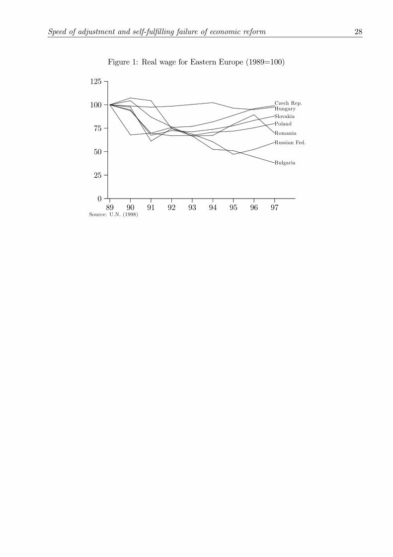
costs are too high. An illustration of the short term cost of transition is given in Figure

1.

Figure 1 about here

The …gure shows the real wage developments in major Eastern European countries

after the break of the wall. The declining real wages in the early 90s stand out as a

common trend in this picture. There is some improvement at the end of the period

in some of these countries. Whether the longer term developments will be signi…cantly


bene…cial for the wage earners is yet to be seen.

Economic reform and income distribution are core issues in development economics,

especially in the study of economies in transition. One central issue is how the speed of

reform may a¤ect the transitional burdens. The contribution of the present work is the

discussion of the political feasibility of reform programmes. The analysis illustrates how

the speed of adjustment a¤ects the severity of transitional burdens, and consequently the

support for reform.

The present example of structural reform is …scal adjustment in a closed economy

consisting of an e¢cient modern private sector, an ine¢cient public sector, and an infor-

mal sector. The …scal adjustment takes the form of laying o¤ public surplus labour and

reducing taxes. The short run e¤ect of the reduction in labour demand is a reduction in

the wage. Reduced wage and reduced taxes increase the return to capital in the modern

private sector. Savings are stimulated and the private capital stock will grow over time,

in a pace determined by the level of savings.1 Labour and capital are assumed to be

strong complements and when the private capital stock grows the wage will recover as

demand for labour increases. The transitional wage movement depends on the speed of

reform. Big bang reform gives a strong wage decline but also a high return to capital.

Hence, the savings response will be strong and the recovery of labour demand is relatively

fast. Gradual reform moderates the immediate wage drop but also slows the recovery.

In the absence of additional constraints, overall e¢ciency is maximized given big bang

removal of the public surplus labour. Fast reform may be infeasible, however, if the re-

quired wage reduction is restricted due to political constraints. In the analysis reform

proposals are assumed to be subject to a vote before implementation. If implementation

implies su¤ering for a substantial section of the population reform is rejected and conse-


cuntly cancelled. In the analysis the exposed group are self-employed unskilled workers in

the informal sector. They are assumed to be pushed below subsistence if labour demand

in the formal part of the economy falls to low. When this constraint is binding big bang

reform will be politically infeasible. A su¢ciently gradual programme, however, will be

feasible as the immideate wage drop is moderated in gradual reform.

The analysis continues by investigating the possibility of self-ful…lling expectations.

In a cancelled reform the future return to capital will be lower than in completed reform.

Expectations about a cancellation will therefore adversely a¤ect savings and investment

and consequently reduce labour demand. The result may be a self-ful…lling failure where

expectations about cancellation itself generate an outcome that causes the cancellation of

reform. Expectations about reform completion, on the other hand, will stimulate invest-

ment and labour demand and may thus generate a self-ful…lling success. The possibility

of dual equilibria depends on the speed of adjustment. Su¢ciently gradual reforms imply

a labour demand during the transition period that is su¢ciently high, independent of

agents’s expectations. The possibility of a vicious circle is thus broken and the reform

is sure to be completed. Su¢ciently gradual programmes have one unique successful

equilibrium. This credibility argument is the second main result.

The linkage between speed of adjustment and popular support is demonstrated in

several countries. One example is Zimbabwe’s structural adjustment programme which

commenced in 1990 with ambitions of a massive reduction in public employment. To date,

only a small fraction of these reductions have taken place, clearly indicating the political

di¢culties of laying o¤ as long as private sector labour demand is far from su¢cient.

Another example is Poland: Following a very ambitious programme, put forward in the

early 1990’s, political unrest was experienced in 1993-1994, delaying both restructuring


and privatization. It is possible that this backlash put the reforms on hold longer than

would have been necessary given a more sober programme.

The present analysis is a stylized description of reform, involving …scal adjustment

and government downsizing. The model may well, however, be directly translated into

other contexts of transition, whether the distinction goes between traded/non-traded,

government/private or exportables/importables. The essential feature that drives the re-

sults is the possibly intolerable transitional burden as the mobilization of capital requires

a high rate of return. In the words of Dornbusch (1990):

What markets consider a su¢cient policy action may simply be beyond

the political scope of democratic governments. In fact, if governments went

far enough to create the incentives that would motivate a return of capital

and the resumption of investments on an exclusive economic calculation, the

implied size of real wage cuts might be so extreme that on political grounds,

asset holders might consider the country too perilous for investment.

Adding to Dornbusch’s argument a mechanism, through which asset holders are com-

pensated for “perilousness” by an even higher rate of return, establishes the possibility

of dual equilibria.

The consequences of a minimum wage on the optimal speed of reform are discussed

among many in Mussa (1986), Torvik(1994) and Mehlum (1998). Further, several works

analyse political constraints to reform and the possibility of reversal. Important contri-

butions have been made by Blanchard et al. (1991) and Krueger (1993). Among the

contributions modelling political support in detail are Rodrik (1995), who explores how

support for reform may change over time as agents …nd themselves among the reform’s


winners or losers. Dewatripont and Roland (1992b) discuss the political economy of tran-

sition from plan to market and …nd that the extent of compensation required increase

with the speed of reform. Roland and Verdier (1994) analyse privatization and …nd crit-

ical mass e¤ects and multiple equilibria, due to externalities and coordination failures.

Multiple equilibria are also a possibility in Rodrik’s (1991) analysis of rational investors’s

response to reform in the presence of policy uncertainty.

Little work has been done linking the speed of reform to the possibility of multiple

equilibria. Frooth (1988) uses a two-period model of trade reform to analyse the possi-

bility of self-ful…lling failure when there are restrictions to international borrowing. The

programme is aborted if the current account balance is su¢ciently worsened. Frooth

…nds that a self-ful…lling failure is most likely given big bang reform.2 This is in contrast

to the conclusion of van Wijnbergen (1992). He analyses the removal of price controls in

a two-period model and …nds that self-ful…lling failure is most likely in gradual reform as

gradualism increses the scope for intertemporal speculation. The opposite conclusions in

the studies by Frooth and van Wijnbergen demonstrates that no general results apply on

this broad issue. The present analysis is similar to these two contributions in the general

spirit. The present focus is essentially di¤erent, however, as it concentrates on functional

income distribution and the accumulation of productive capital. These are crucial factors

for the understanding of the success and failure of the ongoing structural adjustments

e¤orts in many parts of the world. The article is organized as follows: Section 2 and

3 presents the model and the dynamics following economic reform. Section 4 discusses

gradualism versus big bang and the possibility of self-ful…lling failure.


2 The model

The model is in real terms and describes a closed economy. The economy is made up

of three sectors: An ine¢cient public sector, an e¢cient private modern sector, and an

informal sector. The formal part of the economy (the modern sector and the government

sector) is assumed to only employ skilled labour. In the informal sector workers are

unskilled and self-employed.

2.1 The formal sectors

The formal part of the economy has a production structure similar to Castanheira and

Roland’s (1996) dynamic general equilibrium model for economies in transition. While

Castanheira and Roland allow for the public sector to have variable though inferior

productivity, the present assumption is that the public sector is totally unproductive. All

production in the formal part of the economy, Xt, is carried out in the private modern

sector. The modern sector’s factors of production, skilled labour, Lt, and capital, Kt, are

used in …xed proportions with unit coe¢cients. Hence, production at time t is given by

a Leontief function

Xt = min(Lt; Kt) (1)

This production function implies a capital/output ratio of 1. This is consistent with an

implicit assumption about the unit of time being 3 years. This assumption implies a

yearly capital/output ratio of 3, which is in the range of most estimates.

The public sector employs only skilled labour Gt. The total supply of skilled labour,

normalized in size to 1, is fully employed either in the modern or the public sector. Hence,


given the size of public employment, employment in the modern sector is given by

Lt = 1¡Gt (2)

Given the skilled wage, wt, the public wage bill is given by wtGt. Public expenditure is

…nanced through an ad valorem tax, by rate ¿ t, levied on the production of the modern

sector. Assuming that the public budget is in ballance it follows that

wtGt = ¿ tXt (3)

Total production is distributed to skilled workers in the modern and public sector, who

earn the same wage, and to owners of the capital, who receive a constant rate of return

rt on their capital stock

Xt = wt(Gt + Lt) + rtKt (4)

Assuming full capacity utilization in the modern sector (i.e. Xt = Lt = Kt), the equations

(1)-(4) determine X, L, K, w, and ¿ as functions of the policy variable G, and of the

(yet to be determined) interest rate r

Kt = (1¡Gt) (5)

Xt = (1¡Gt) (6)

wt = (1¡ rt)(1¡Gt) (7)

¿ t =wtGtXt

= (1¡ rt)Gt (8)


Full capacity utilization implies that increasing public employment reduces the private

capital stock 1 to 1. The public sector is not contributing to the generation of values hence

production and wages decrease as well. The wage level also declines when the interest

rate increases. Lastly, the tax rate increases with the public wage bill and declines with

increased production.

2.2 The informal sector

The informal part of the economy is modelled as simple as possible. Entry into the sector

is free and production is given by the production function Y (N), where N is the number

of self-employed unskilled workers. The informal wage ° is assumed to be given by the

average productivity of labour

° = Y (N) =N

Assuming decreasing return to scale in infomal sector, the informal wage will decline in

the number of self-employed workers. Self-employment in the informal sector is assumed

to be the only option for the unskilled workers and they are assumed not to have access

to credit. It is further assumed that the informal wage ° is at the level of subsistence

when only unskilled are self-employed.3

The skilled workers will shun self-employment as long as w > °. If the demand

for labour in the formal sector is su¢ciently low, however, self-employment will be an

attractive option also for the skilled workers. Hence, ° represents a lower boundary for the

wage ‡exibility in the formal sector. A w below ° will generate a ‡ow of skilled workers

into self-employment that push the wage in the informal sector down below subsistence.

Hence, reforms implying w < ° will imply starvation for the unskilled workers and is


in the following assumed to be infeasible due to political constraints. The conditions

underlying these political constraints are discussed thoroughly below. Before going in

detail on feasibility of reform the dynamics of the model must be determined.

2.3 The dynamics of the model

In order to solve the model the interest rate must be determined. The supply of savings is

determined by dynamically optimizing agents, all having access to a perfect credit market.

These agents, the skilled labour, maximize an unit elasticity CRRA utility function with

discount factor µ, giving individual (indexed by i) utility

Ui =

1Xt=0

µ1

(1 + µ)tln (Ci;t)

¶(9)

Given (9), the Ramsey rule4 gives agent i’s consumption path as follows

Ci;t+1 =1 + rt+11 + µ

Ci;t (10)

Summing all agents, it follows that the aggregate consumption path has the same growth

rate as the individual consumption paths

Ct+1 =1 + rt+11 + µ

Ct (11)

Abstracting from depreciation, and ruling out in‡ow of capital from abroad,5 accu-

mulation of the economy’s only asset, physical capital, is given by savings, S. Since the

unskilled workers are excluded from the credit market the entire product of the informal


sector will be consumed. It follows that Kt+1 ¡Kt = S = X ¡ C and hence

Kt+1 = Kt +Xt ¡ Ct = Kt + St (12)

The di¤erence equation (11) determines consumption and thus, combined with (12), the

supply of capital over time. The supply of capital is determined by domestic savings and

is thus a function of the interest rate. From the Leontief production function it follows

that demand for capital will be determined solely by the number of skilled labourers

available for the formal sector. Given the level of public employment demand for capital

will be inelastic and the equilibrium interest rate will be determined by supply.

The present model is in this respect di¤erent from the standard Ramsey formula-

tion where the demand for capital gradually declines as the marginal return of capital

asymptotically approaches zero. One familiar implication of this smoothly decreasing

demand for capital is the asymptotic transition path. In the present model, zero-elastic

capital demand implies that the stock of capital adjusts fully in …nite time. Following

any exogenous shock, the new steady state will be reached over only one period.6 This

property substantially simpli…es the solution of the model. Even though the agents live

for ever and have perfect foresight, the number of transition periods is limited and exact

closed form solutions can be found for all variables.

Following from (6), changing public employment will shift the steady state and in-

duce transition. Reduced public employment increases the labour available for the private

sector and increases the demand for capital. During transition to a higher level of pro-

duction, the rate of interest will be high and savings will be positive.

Given the development in public employment (: : : ; Gt¡1; Gt; Gt+1; : : : : ), the paths for


the endogenous variables follow from the model above. Inserting (6) and (5) in (12) gives

Ct = 1¡ 2Gt +Gt+1 (13)

inserting in (11) and solving for rt gives

rt = (1 + µ)1¡ 2Gt +Gt+11¡ 2Gt¡1 +Gt ¡ 1 (14)

inserting in (7) gives

wt = (1¡ rt)(1¡Gt) =µ2¡ (1 + µ)1¡ 2Gt +Gt+1

1¡ 2Gt¡1 +Gt

¶(1¡Gt) (15)

Steady state is characterized by Gt¡1 = Gt = Gt+1. It is readily seen from (14) and (15)

that the steady state values of interest rate and skilled wage are given by rt = µ and

wt = (1¡ µ)(1¡Gt).

3 Economic reform

Consider the case where the economy is in a steady state with a level of public employment

G0 > 0. Then, in Period 0 the government decides to remove this public sector surplus

labour. Their announcement is unexpected as it for example follows the break of the wall

or a surprise agreement with the IMF. At this point in time the size of G0 is determined.

The reform will thus materialize at the earliest in Period 1 by a reduction in G1. Hence,

the historically determined X0, r0, and w0 will not be a¤ected. S0, C0, and r1, however,

will deviate from their historic steady state levels as demand for capital in Period 1

increases following the reduction in G1.


For expositional clarity, public employment is assumed to be reduced to zero over

at most two periods, G0 > G1 ¸ G2 = 0. As G0 is determined by history and with

G2 = 0 as the target, the various programmes will only di¤er in their speed, captured

by the size of G1. The case where public employment is set to zero already in Period

1 (G1 = 0) is the big bang case, while the case where public employment is reduced

stepwise (G1 > 0) is labelled gradualism. Inserting the public employment path in (14)

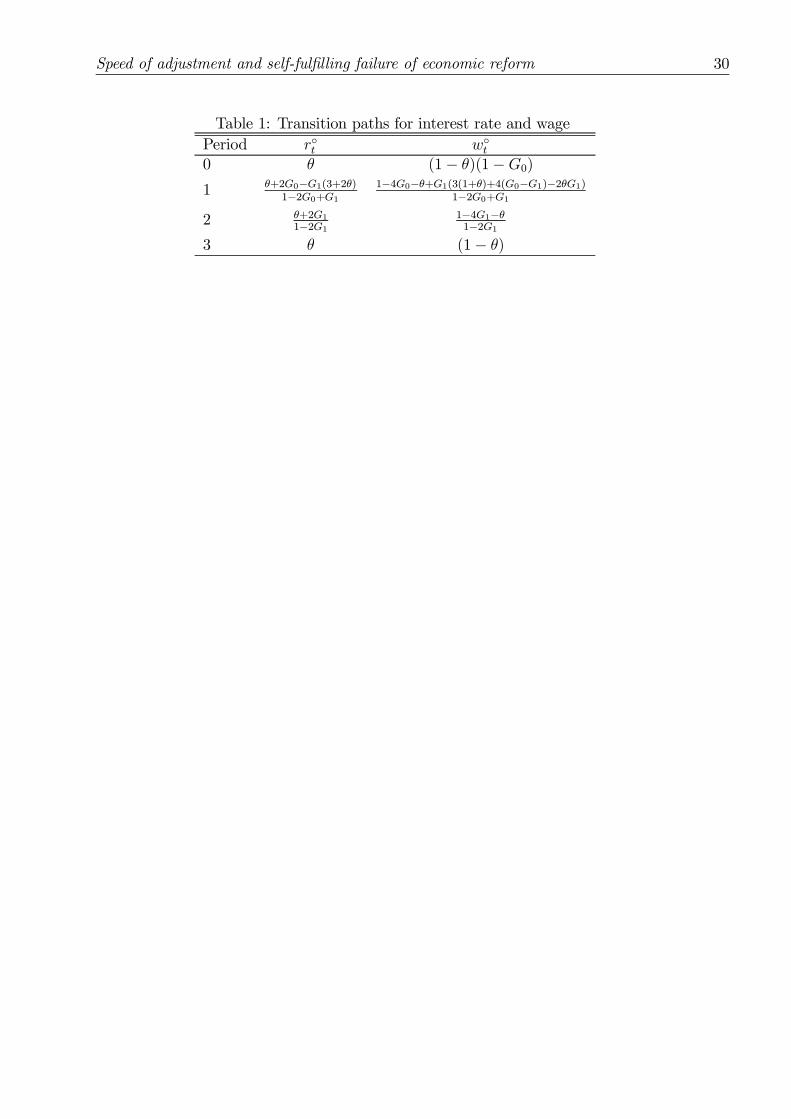
and (15), and assuming fully ‡exible factor prices,7 the equilibrium values r±t and w±t over

the transition periods follows in Table 1.

Table 1 about here

As noted above, in steady state rt = µ and wt = (1¡ µ)(1¡Gt). This basic result is

re‡ected also in Table 1. The economy starts out at the historic steady state in Period

0 and ends up in the new steady state in Period 3. The shape of this over-all movement

is a¤ected by the speed of reform, i.e. the size of G1.

Big bang reform implies an instant removal of public employment (G1 = 0) Inserting

in Table 1 it follows8 that w±1 < w±0 < w

±2 = w

±3 and that r

±1 > r

±0 = r

±2 = r

±3 = µ. That

is, the wage follows a J-curve, falling before …nally settling at a higher level, while the

interest rate goes through a transitional hump before returning to the steady state level.9

Given gradual reform (G1 > 0) the mobilization of private capital is carried out over two

periods. The required adjustment is less abrupt, the transition paths are smoothed, and

steady state is not reached until Period 3. w1 will be higher while w2 will be lower than

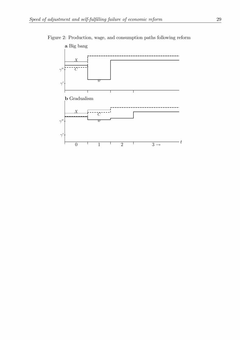
in big bang. These transition paths, in addition to production and consumption paths,

are illustrated in Figure 2, with the big bang in the upper panel and one gradual case in


the lower.10 Production and consumption are given by thin and dashed line respectively

and follow directly from (6) and (13).

Figure 2 about here

Figure 2 illustrates the arguments above: The big bang wage path goes through a steep

decline in the …rst transition period, recovers rapidly, and settles at the new and higher

steady state level in Period 2. In a gradual reform process the wage path is smoother.

The initial wage drop is less, but the recovery is slower.11 In both cases the short run

e¤ect of reform is a reduction in the wage. Reduced wage and reduced taxes, however,

increases the return to capital. Savings are stimulated and the private capital stock will

grow over time, in a pace determined by the level of savings. As Labour and capital are

strong complements the wage will recover as the private capital stock grows. Big bang

reform gives a strong wage decline but also a high return to capital. Hence, the savings

response will be strong and the recovery of labour demand is relatively fast. Gradual

reform moderates the immediate wage drop but also slows the recovery.

Given the menu of reform alternatives G1 2 [0; G0], the actual reform design will be

determined by policy-makers ambitions and political constraints. In the following section

an agenda-setting government framework à la Romer and Rosenthal (1979), adopted

from Dewatripont and Roland (1992a), is introduced: Reform plans are proposed by the

government who is assumed to be in control of the agenda of reform proposals, but these

proposals are, however, subject to political constraints. In this context, we assume that a

majority (or even unanimity) of workers is required to approve a reform plan prior to its

implementation.(p.292)


3.1 The agenda-setting government and political constraints

The reform-minded government is assumed to propose a reform plan with the objective

of maximizing over all e¢ciency. As production in the informal economy is constant this

implies the maximization of formal sector productionX. The government …rst announces

the plan that subsequently is subject to a vote. If the plan is approved, the reform is

completed as announced. If not, the reform is cancelled and the economy is left at status

quo.

Looking only at the formal sectors it is clear that big-bang reformmaximizes e¢ciency.

As the skilled labour own all the capital they will gain from, and therefore support, fast

reform. For the unskilled workers the critical condition is whether w remains above °

throughout the transition process or not. As long as w > ° the number of self-employed

workers remains …xed and they will continue to enjoy their subsistence consumption

level °. They will thus be indi¤erent between reform and status quo. If, however, the

transition is too fast w will be pushed down to °, skilled workers will enter into self-

employment and consequently unskilled consumption will be pushed below the level of

subsistence. Figure 2 includes two alternative levels of °. When ° is low (°0) the skilled

wage w will be above ° even for the big bang reform and the unskilled workers will not

be hurt during transition . When ° is high (°00) big bang reform will require a w below

the skilled workers subsistence.12 A su¢ciently gradual reform, however, will go clear of

this limit. Hence, in the case of ° = °00, big bang implies starvation for the unskilled

workers and they will strongly oppose reform.

The outcome of the vote over reform depends both on the number of unskilled workers

and on the assessment of the skilled workers. The opposition towards speedy reform will

be su¢cient to give reform cancellation if 1) the unskilled represents the majority, 2)


there is su¢cient altruism towards the starving, or 3) when the starving are likely to

destabilize the economy, generating an inferior outcome for all. In the following it is

assumed that at least one of these conditions are satis…ed. Hence, a drop in the skilled

wage below ° will not be politically feasible. The outcome of the reform vote is formally

speci…ed as follows: Reform is approved if and only if wi ¸ ° i = 1; 2.

Taking this political constraint into account, a reform-minded government will only

announce feasible programmes. That is, programmes su¢ciently gradual to assure a

market clearing formal wage above the wage in the informal part of the economy. This

leads to the feasibility argument for gradualism:

² Given a subsistence consumption constraint big bang reform, leading to a strong

reduction in wages, may be politically infeasible. Gradualism then represents a

feasible reform alternative.

The analysis above does not explicitly discuss transfer schemes to compensate losers.

The present argument for gradualism may, however, be translated into an argument

for an unemployment bene…t. The results above would also be valid given a transfer

scheme where G1 is interpreted as skilled workers receiving bene…t w1 instead of being

public employees producing nothing and receiving wage w1. This does not rule out that

other transfer schemes may be more e¢cient than gradualism. However, asymmetric

information, intertemporal commitment problems and other distortions generally limit

the scope for targeted compensation schemes.

3.2 Credibility and self-ful…lling failure

The analysis above was done under the assumption that the reform was sure to be

approved given that it was feasible. As will be shown in this sub-section this condition


is not su¢cient. Also ex ante feasible programmes may generate an excessive wage drop

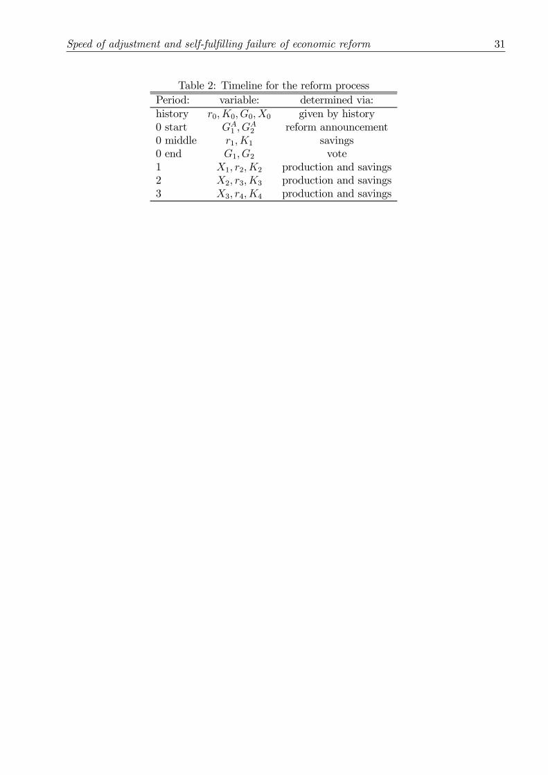
due to self-ful…lling mechanisms. Before going in details, the status quo and the timing

of events will be explicitly speci…ed.

Given the Leontief production function and the wage constraint an over-night …ring

of government workers can be ruled out. The accumulation of capital, required to hire

the …red workers, takes time. Therefore a reform programme, which starts in Period 1,

G0 > GA1 ¸ GA2 = 0 must be announced (A indicates announcement) at the beginning of

Period 0 in time have impact on labour demand in Period 1. The critical vote is assumed

to be carried out at the end of Period 0, just before the actual reform implementation. At

this point in timeK1 is determined and the actual consequences of reform implementation

can be observed by the voters. If, for example, K1 < 1¡GA1 reform implementation will

imply that skilled workers enter into self employment. That in turn implies starvation

for the unskilled workers and reform implementation will therefore be voted down. If

the reform is rejected, the following status quo policy is implemented: Firing of public

workers is brought to the point assuring w1 ¸ ° (that is G1 = 1¡K1) and the programme

is put on hold for the ensuingperiods.13 Hence status quo implies

G1 = 1¡K1 > GA1 and G2 = G1

The sequencing of events is summarized in Table 2.

Table 2 about here

Cancelled reform is characterized by G2 = G1, in contrast to completed reform where

G2 = 0. Rational agents with perfect foresight will incorporate the possibility of cancella-


tion in their decision making. Solving (15) and (14) given G2 = G1 gives the transitional

development for interest rates and wages in cancelled reform. The results are summarized

in Table 3, where superscript ¤ indicates cancelled and ± completed (as in Table 1)

Table 3 about here

By comparing the outcome of completed and cancelled reform it becomes clear that

r¤1 ¸ r±1 and r¤2 · r±2 while w

¤1 · w±1 and w

¤2 ¸ w±2. The explanations are as follows: In

a cancelled programme there is no savings in Period 1, hence r¤2 · r±2. Consumption in

Period 1 will therefore be higher than in the completed programme, hence r¤1 ¸ r±1 The

e¤ects on wages follow from these interest rate e¤ects, combined with the lower level of

production from Period 2 and onwards, given cancellation.

As G1 approaches zero the di¤erence between completion and non-completion disap-

pears. The reason is simple enough. When G1 is close to zero the programme is close

to being a big bang programme and, as the big bang programme is …nalized by the end

of Period 1, a cancellation has no e¤ect. The di¤erence between Period 1 wage, given

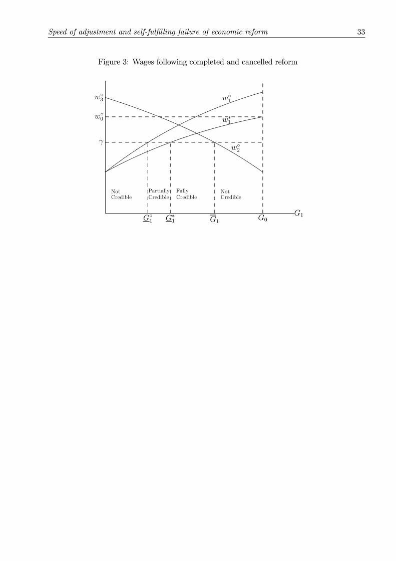
completion, w±1, and given cancellation, w¤1, is illustrated in Figure 3.

Figure 3 about here

The curves w±1 and w¤1 represent the transitional wage given expectations about com-

pletion and cancellation respectively. Adding to this the condition that reform is rejected

and cancelled if the equilibrium wage falls short of °, gives rise to multiple equilibria.

The lowest feasible G1 given expectations about completion is G±1. The lowest feasible

G1 given cancellation is G¤1.


Programmes in the range GA1 < G±1 are rejected and cancelled no matter what the

agents expect. Rational agents will therefore expect a cancellation. The same is true for

programmes in the range GA1 > G1 that gives a skilled wage short of ° in Period 2. Using

the terminology of Sachs et al. (1996), these programmes are not credible. Programmes

in the range G¤1 < GA1 < G1 are fully credible. They are approved no matter what the

agents expect, rational agents will therefore expect completion. Programmes in the range

G±1 < G1 < G¤1 will be approved and completed only if the agents expect a completion

and cancelled if the agents expect a cancellation.14 This intermediate interval is thus

characterized by multiple equilibria and is therefore only partially credible:15

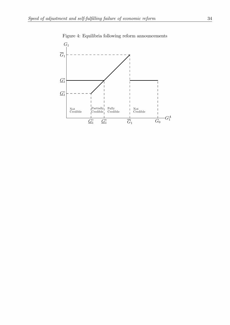
An alternative view of the credibility regions, clearly displaying the two equilibrium

arms, are given in Figure 4. Here, the reform announcement, GA1 , is given along the

horizontal axis and the actual outcome along the vertical axis.

Figure 4 about here

Approved programmes are found along the 45±-line where the outcome is as announced,

G1 = GA1 . Cancelled programmes are given by G1 = G¤1 (the condition that assures

w1 = °)

Reform announcements to the left of G±1 are bound to fail, hence the outcome is G¤1.

Reform announcements between G¤1 and G1 are bound to succeed, hence the outcome is

G1 = GA1 . For programmes G

±1 < G

A1 < G

¤1 there are two options: Self-ful…lling success,

G1 = GA1 , or self-ful…lling failure, G1 = G

¤1. The possibility of multiple equilibria modi…es

the simple policy lesson from above - that programmes not should be faster than G±1. An

intermediate range exists where failure is possible due to self-ful…lling mechanisms. Only


su¢ciently gradual programmes are sure to succeed. This second main result adds to the

feasibility argument given above and can be formulated as follows:

² Self-ful…lling expectations can cause both failure and success of reform. The possi-

bility of such dual equilibria depends on the speed of reform. Su¢ciently gradual

programmes have one unique successful equilibrium.

Given that big bang reform forces the unskilled workers below subsistence reform

must be gradual in order to be feasible. Reform must be even more gradual, however, in

order to be fully credible. If the government has means to convince all agents that the

programme will be completed, credibility is not an issue, and the optimal programme

is the one that just steers clear of the minimum wage constraint. Without such means,

pessimistic rational agents may generate self-ful…lling cancellation. The only way to

avoid this possibility of a vicious circle is to play safe and propose an even more gradual

programme.

Another possibility could be to shift the date of the vote forward in time. In that

case the decisions of the voters would be known when the investment decisions are made.

The mechanisms through which the self-ful…lling expectations worked is then cut o¤ and

the problem would be solved. The condition for this solution is that there is no vote in a

certain time span around the beginning of period 1. This may not be feasible however.

Given the far-reaching transitions presently considered, the critical time span would be

several years long and cancelling votes/elections for years would require authoritarian

rule.16 Furthermore, even in the case where a formal vote were avoided, a starving

population could force an informal `vote’ by destabilizing the economy and force the

government to cancel the reform.


All the results above are achieved under a moderate cancellation assumption. Rodrik

(1991) has an alternative assumption where reform failure implies a complete return to

the pre-reform policy and hence reversal of investments. Applying this radical assumption

would reinforce the present self-ful…lling mechanism as cancellation would imply an even

stronger fall in capital return. Adding also, as Rodrik, irreversibility of investments would

strengthen the results even further.

4 Conclusion

The possibility of failure of a reform programme depends on the degree of gradualism

in the announced reform plan. Two arguments for gradualism are made. First, a rapid

transition requires a high interest rate and a low transitional wage. A subsistence con-

sumption constraint limits the feasible wage drop and determines the maximum speed of

transition. Reform programs faster than this limit, e.g. big bang reform, are bound to

fail. Second, agents’s expectations about failure may prove self-ful…lling. The existence

of multiple equilibria is dependent on the degree of gradualism of the reform. Su¢ciently

gradual programmes have one unique, successful, equilibrium.

These results, following from the interplay between e¢ciency, income distribution and

political constraints, are achieved in a stylized general equilibrium model. The transpar-

ent analysis reveals important mechanisms that will also be present in other models.

The essential linkages underlying the results are: 1) the capital accumulation is in‡u-

enced both by present and expected future return, 2) fast reform lowers the transitional

wage, 3) a political constraint that a¤ects the future return on capital, and 4) forward-

looking agents. This set of features is clearly not con…ned to the present model. Hence,

the Ramsey consumer and Leontief production function may be replaced by alternative


assumptions without a¤ecting the qualitative results. Consider, for example, the produc-

tion structure. The essential property is the immediate real wage drop following reform.

This wage drop is generally only avoided in models which either allow for a high degree

of substitution between factors of production or where a substantial stock of capital is

made available from the contracting sector. In these cases, labour will have high marginal

productivity also in the short run, and the wage drop can be avoided. As Figure 1 clearly

demonstrates, however,a real wage drop is rather a rule than exception in economies of

transition.

The transition process would also be helped by a substantial in‡ow of foreign in-

vestments at the early stage of reform. This could be achieved in a model allowing for

international capital mobility. International investors would be attracted by the high

return to capital but they are also sensitive to political risk. Their involvement could

thus exacerbate, instead of alleviating, the problem of self-ful…lling expectations. Less

risk conscious investors or economic aid, however, could remove the pivotal role play by

expectations and generate a predictable reform success.

References

Alesina, A. and A. Cuikerman, 1990, The politics of ambiguity, Quarterly Journal of

Economics, Vol:CV, 4, 829-51.

Blanchard, O., R. Dornbusch, P. Krugman, R. Layard and L. Summers, 1991, Reform in

Eastern Europe (MIT Press, Cambridge, Mass.)

Bu¢e, E. F., 1995, Trade liberalization, credibility and self-ful…lling failures, Journal of

International Economics, 38, 51-73.


Castanheira, M. and G. Roland, 1996, The optimal speed of transition: A general equi-

librium analysis, CEPR Discussion Paper No. 1442.

Dornbusch, R., 1990, Policies to move from stabilization to growth, World Bank Confer-

ence on Development Economics, Proceedings 1990, 19-48.

Dewatripont, M. and G. Roland, 1992a, The virtues of gradualism and legitimacy in the

transition to a market economy, Economic Journal, 102, 291-300.

Dewatripont, M. and G. Roland, 1992b, Economic reform and dynamic political con-

straints, Review of Economic Studies, 59, 703-730.

Frooth, K. A., 1988, Credibility, real interest rates, and the optimal speed of trade

liberalization, Journal of International Economics, 25, 71-93.

Krueger, Anne O., 1993, Political pconomy of policy reform in developing countries. (MIT

Press, Cambridge Mass.)

Mehlum, H., 1998, Why gradualism?, Journal of International Trade and Economic De-

velopment, 7:3, 279-297.

Mehlum, H., 1999, The political economy of failing reform, Phd thesis, (Department of

Economics, University of Oslo).

Mussa, M., 1986, The adjustment process and the timing of trade liberalization, in:

Choksi, A. M. and D. Papageorgiou, eds., Economic liberalization in developing

countries, (Basil Blackwell, New York).

Rodrik, D., 1991, Policy uncertainty and private investment in developing countries,

Journal of Development Economics, 36, 229-242.


Rodrik, D., 1995, The dynamics of political support for reform in economies in transition,

Journal of Japanese and International Economies, 9, 403-425.

Roland, G. and T. Verdier, 1994, Privatization in Eastern Europe: Irreversibility and

critical mass e¤ects, Journal of Public Economics, 54 161-183

Romer, T. and H. Rosenthal, 1979, Bureaucrats versus voters: On the political econ-

omy of resource allocation by direct democracy, Quarterly Journal of Economics,

93(4)563-587.

Sachs, J, Tornell, A, and Velasco A., 1996, The Mexican peso crisis: Sudden death or

death foretold?, Journal of International Economics, 41, 265-283.

Schmidt-Hebbel et al., 1996, Saving and investment: Paradigms, puzzles, policies, The

World Bank Research Observer, 11(1), 87-117

Takayama, A, 1993, Analytical Methods in Economics, (The University of Michigan

Press, Ann Arbor).

Torvik, R., 1994, Trade Policy under a Binding Foreign Exchange Constraint, Journal of

International Trade and Economic Development, 3, 15-31.

U.N., 1996, Economic Survey of Europe in 1995-1996, (United Nations, New York and

Geneva).

van Wijnbergen, S., 1992, ,Intertemporal Speculation, shortages and the political

economy of price reform, The Economic Journal, 102, 1395-1406.


Notes

1As the economy is closed investments is determined by the level of domestic sav-

ings. Implications from allowing for ‡exible in- and out‡ow of capital is discussed in

the concluding section. As pointed out in a study by Schmidt-Hebbel et al (1996 p.

93), however, the assumption about constrained access to foreign …nancing is realistic for

many developing countries: `In the extreme situation of low (or zero) access to foreign

capital, a condition faced by many developing countries during 1980s, national saving

and domestic investment will be highly (indeed perfectly) correlated.’

2A continous time model with similar mechanisms and results is used by Bu¢e (1995).

3The assumption about ° being exactly the subsistence consumption level is mainly a

conseptional simpli…cation. It alows me to talk about starvation as soon as the unskilled

wage falls short of °.

4See for example Takayama (1993)

5Implications from allowing for in- and out‡ow of capital is discussed in the concluding

section.

6This is under the condition that the required changes are physically possible.

7The subsistence constraint w ¸ ° will be discussed in detail below.

8Given the natural limitations C1 > 0 and w1 > 0 for G1 = 0, it follows from

w1 = (1¡ 4G0 ¡ µ) = (1¡ 2G0) that reforms under consideration must commence at

G0 < (1¡ µ) =4.

9The initial downturn of wages implies that the relative factor price shift in the dis-


favour of labour dominates the e¢ciency gain. This result may be altered if the in-

tertemporal elasticity of substitution in consumption is increased from its assumed level

of one. It is easily shown, however, that an overnight removal of government employment

inevitably gives reduced wage in the corresponding continous time model, irrespective

of the intertemporal elasticity of substitution. As the present model is a discrete time

approximation to this continous time reality, it is essential that it re‡ects the feature of

wage drop following big bang.

10The numerical example is based the following parameter values (to be used through-

out the paper): µ = 1=8, G0 = 1=6. Note that the implicit assumption about a period

length of three years implies a year by year discount factor of µ=3 = 4:2%.

11A complete picture of the transitional wages, w±1 and w±2, is given in Figure 3 below.

12It should be noted that the equilibrium wage in Table 1, in Figure 2, and in the

following …gures are calculated under the assumption that L = 1 ¡ G. Thus, the im-

plication for the formal labour supply, when skilled workers enter into self-employment

as w < °, is not accounted for. In an all-inclusive calculation the wage drop would be

somewhat moderated as soon as the constraint w = ° was broken. This modi…cation do

not alter the essential result that unskilled labour is pushed below subsistence for any

reform requiring w < °.

13Note that the status quo is moderate as it does not imply a restoration of the historic

public employment G0. The downsizing of the government is brought to the point made

possible by the private investments already made, but further reductions are not made.

This …ts well with observations from Eastern Europe where political backlashes take the

form of freezing of the reform proceses rather than a complete return to the historic state.


14The equilibrium concept is Nash equilibrium with all agents as players and with full

information. Hence, equilibrium requires concurrent expectations, ruling out solutions

where one fraction expects cancellation and the other completion.

15As ° increases, the fully credible range gets smaller, and for su¢ciently high °, no

fully credible two period reform exists. The reform will then have to go over three or

more periods. This case will not be discussed, but it is a straight forward extension of

the present analysis.

16This issue is discussed at length in Mehlum (1999).


Figure 1: Real wage for Eastern Europe (1989=100)

89 90 91 92 93 94 95 96 970

25

50

75

100

125

Source: U.N. (1998)

......................................................................................................................................................................................................................................................................................................................................................................................................................................................................................................................................................................................................................................................................................................................................................................Bulgaria

.......................................................................................................................................................................................................................................................

...................................................................................................................

..............................................................

.................................................

............................................

............................................

...........................................

..................................................................................

Czech Rep.............................................................................................................................................................................................................................................................................................................................................................

...............................................................................................................................................................................................................................................................................................Hungary

..........................................................................................................................................................................................................................................................................................................................................................................................................................

............................................................................................................................................

...............................................................................

................................................................

..Poland

...................................................................

......................................................................................................................................................................................................................................................................................................................................................................................................................................................................................................................................................................................................................................................................Romania

..........................................

..........................................................................................................................................................................................................................................................................................................................................................................................................................................................................................................................................................

.........................................................

..........................................

.....................................Russian Fed.

...........................................................................................................................................................................................................................................................................

........................................................................................................................................................................................................

........................................................................

....................................................

..............................................................

.................................Slovakia


Figure 2: Production, wage, and consumption paths following reform

b Gradualism

°00

°0

t0 1 2 3!

XC

w

a Big bang

°00

°0

X

C

w


Table 1: Transition paths for interest rate and wagePeriod r±t w±t0 µ (1¡ µ)(1¡G0)1 µ+2G0¡G1(3+2µ)

1¡2G0+G11¡4G0¡µ+G1(3(1+µ)+4(G0¡G1)¡2µG1)

1¡2G0+G12 µ+2G1

1¡2G11¡4G1¡µ1¡2G1

3 µ (1¡ µ)


Table 2: Timeline for the reform processPeriod: variable: determined via:history r0; K0; G0; X0 given by history0 start GA1 ; G

A2 reform announcement

0 middle r1; K1 savings0 end G1; G2 vote1 X1; r2; K2 production and savings2 X2; r3; K3 production and savings3 X3; r4; K4 production and savings


Table 3: Transition paths for interest rate and wage in cancelled reformPeriod r¤t w¤t0 r±0 w±0

1 r±1 +G1(1 + µ)

1¡ 2G0 +G1 w±1 ¡G1(1 + µ)(1¡G1)1¡ 2G0 +G1

2 r±2 ¡ 2G1(1 + µ)

1¡ 2G1 w±2 +G12(1¡ µ)G1 + 1 + 3µ

1¡ 2G13 r±3 w±3 ¡ (1¡ µ)G1


Figure 3: Wages following completed and cancelled reform

G1G0G±1 G¤1 G1

°

w±0

w±3 w±1

w±2

w¤1

...........................................................................................................................................................................................................................................................................................................................................................................................................................................................................................................................................................................................

..........................................

..............................................

....................

..............................................................................................................................................................................................................................................................................................................................................................................................................................................................................................................................................................................................................................................................................................................................................................................................................................................................................................................................................................................................................................

............................................

.............................................

..................................................

.....................................................

...........................................................

..................................................................

...

NotCredible

PartiallyCredible

FullyCredible

NotCredible


Figure 4: Equilibria following reform announcements

GA1

G1

G0G±1

G±1

G¤1

G¤1

G1

G1

.....................................................................................................................................................................................................................................................................................................................................................................

..................................................................................................................................................................................................................................................... ......................................................................................................................................................................................

NotCredible

PartiallyCredible

FullyCredible

NotCredible

speed of adjustment and self-ful…lling failure of...

Documents