sphere tracing: a geometric method for the antialiased ray...
TRANSCRIPT

Sphere Tracing: A Geometric Method for the
Antialiased Ray Tracing of Implicit Surfaces�
John C. Hart
School of EECS
Washington State University
Pullman, WA 99164-2752
(509) 335-2343
(509) 335-3818 (fax)
Abstract
Sphere tracing is a new technique for rendering implicit surfaces using geometric distance.
Distance-based models are common in computer-aided geometric design and in the modeling
of articulated figures. Given a function returning the distance to an object, sphere tracing
marches along the ray toward its first intersection in steps guaranteed not to penetrate the
implicit surface.
Sphere tracing is particularly adept at rendering pathological surfaces. Creased and rough
implicit surfaces are defined by functions with discontinuous or undefined derivatives. Current
root finding techniques such as L-G surfaces and interval analysis require periodic evaluation
of the derivative, and their behavior is dependent on the behavior of the derivative. Sphere
tracing requires only a bound on the magnitude of the derivative, robustly avoiding problems
�Manuscript, July 1994. Recommended for publication: The Visual Computer.
5-70

where the derivative jumps or vanishes. This robustness and scope support sphere tracing as an
efficient direct visualization system for the design and investigation of new implicit models.
Furthermore, sphere tracing efficiently approximates cone tracing, supporting symbolic-
prefiltered antialiasing. Signed distance functions for a variety of primitives and operations
are derived and appear independently as appendices, specifically the natural quadrics and
torus, superquadrics, Bezier-based generalized cylinders and offset surfaces, constructive solid
geometry, pseudonorm and Gaussian blends, taper, twist and hypertexture.
Keywords: area sampling, blending, deformation, distance, implicit surface, Lipschitz condition,
numerical methods, ray tracing, solid modeling.
1 Introduction
Whereas a parametric surface is defined by a function which, given a tuple of parameters, indicates
a corresponding location in space, an implicit surface is defined by a function which, given a point
in space, indicates whether the point is inside, on or outside the surface.
The most commonly studied form of implicit surfaces are algebraic surfaces, defined implicitly
by a polynomial function. For example, the unit sphere is defined by the second degree algebraic
implicit equation � 2 + � 2 + � 2 � 1 = 0 (1)
as the locus of coordinates whose hypotenuse (squared) is unity.
Alternatively, using a distance metric, one can represent the unit sphere geometrically by the
implicit equation ��� ����� � 1 = 0 (2)
as the locus of points of unit distance from the origin. Here�
= ( �� � � � ) and��( �� � � � )
��denotes
the Euclidean magnitude � � 2 + � 2 + � 2 � The implicit surface of (2) agrees with that of (1), though
their values differ at almost every other point in 3 � Specifically, (1) returns algebraic distance
[Rockwood & Owen, 1987] whereas (2) returns geometric distance.
5-71

A comparison of geometric versus algebraic representations of quadric surfaces preferred the
geometric representation [Goldman, 1983]. The parameters of a geometric representation are
coordinate-independent, and are more robust and intuitive than algebraic coefficients. Distance-
based functions like (2) are one method for representing implicit surfaces geometrically.
Distance-based models can be found in a variety of areas. Offset surfaces have become valuable
in computer-aided geometric design for their use of distance to model the physical capabilities of
machine cutting tools [Barnhill et al, 1992]. Skeletal models, which in computer graphics simulate
articulated figures such as hands and dinosaurs, are equivalent to offset surfaces. Computer vision’s
medial-axis transform converts a given shape to its skeletal representation [Ballard & Brown,
1982]. Generalized cylinders began as a geometric representation in computer vision [Agin &
Binford, 1976] but have also matured into a standard modeling primitive in computer graphics
[Bloomenthal, 1989] --- special ray tracing algorithms were developed for their rendering in [van
Wijk, 1984; Bronsvoort & Klok, 1985].
1.1 Previous Work
Several methods exist for rendering implicit surfaces. Indirect methods polygonize the implicit
surface to a given tolerance, allowing the use of existing polygon rendering techniques and hardware
for interactive inspection [Wyvill et al, 1986; Bloomenthal, 1988]. Although polygonization
transforms implicit surfaces into a representation easily rendered and incorporated into graphics
systems, polygonizations are typically not guaranteed and may not accurately detect disconnected
or detailed sections of the implicit surface. Production ray tracing systems tend to polygonize
surfaces, resulting in large time and memory overhead to accurately represent an otherwise simple
implicit model.
In an effort to combine speed and accuracy, [Sederberg & Zundel, 1989] developed a direct
scan-line method to more accurately render algebraic implicit surfaces at interactive speeds. Ray
tracing, on the other hand, is a direct, accurate and elegant method for investigating a much larger
variety of implicit surfaces.
5-72

Let� ( � ) = ��� +
� ��� (3)
parametrically define a ray anchored at � � in the direction of the unit vector � � � Plugging the ray
equation � : �� 3 into the function � : 3 � that defines the implicit surface produces the
composite real function : � where = ��� � such that the solutions to
(�) = 0 (4)
correspond to ray intersections with the implicit surface. Implicit surface ray-tracing algorithms
simply apply one of the multitude of numerical root finding methods to solve (4).
When � (�
) = 0 implicitly defines an algebraic surface, (4) is a polynomial equation. Analytic
solutions exist for polynomials of degree four or less, but may not be the best numerical method in
certain cases. In this and higher degree cases, solving requires an iterative root finding algorithm.
Some algebraic surface renderers have used DesCartes’ rule of signs [Hanrahan, 1983], Sturm
sequences [van Wijk, 1984], and Laguerre’s method [Wyvill & Trotman, 1990], which capitalize
on properties of polynomials, and are hence more efficient than general root finders.
One must use a general root finder to render the implicit surface of an arbitrary function.
Ideally, this root finder should only need the ability to evaluate the function at any point. However,
one can always construct a pathological function that will cause such a ‘‘blind’’ technique to miss
one or more roots, by inserting an arbitrarily thin region between samples where the function zips
off to zero and back (a point reiterated from [Kalra & Barr, 1989; Von Herzen et al, 1990]). Hence,
any robust root finder needs more information than simple function evaluation.
The ‘‘Hypertexture’’ system used a brute-force blind ray-marching scheme, using only function
evaluation [Perlin & Hoffert, 1989]. Its lack of robustness required fine sampling along the ray,
resulting in rendering speeds so slow they demanded parallel implementation. Requiring only
function evaluation allowed the design of implicit surfaces without regard to the analytic properties
of their defining functions. Freed from such constraints, fractal and hairy surfaces were easily
modeled by implicit surfaces whose functions contained procedural elements.
Robust ray intersection requires extra information, which in most cases is produced by the
derivative of the function. Current techniques repeatedly subdivide the graph of (�) until it is
5-73

partitioned into intervals that either do not intersect the�-axis, corresponding to no ray intersection,
or the graph of the derivative �(�) does not intersect the
�-axis, corresponding to only one ray
intersection. The root within such an interval is refined using Newton’s method and regula falsi. In
the rare case of a multiple root, such as when a ray grazes a surface or intersects coincident surfaces,
the root isolation process subdivides the interval surrounding the root to machine precision.
Interval analysis finds ray intersections by defining the function and its derivative on intervals
instead of single values. It uses such interval arithmetic operations to bound the values of and
its derivative � � Over an interval, if the bound of omits zero, then there is no root. Otherwise if
the bound of �omits zero, then there is a single root. Otherwise the interval is subdivided at its
midpoint [Mitchell, 1990b].
Lipschitz methods are an alternative to interval analysis. (Lipschitz and interval methods are
compared in Section 2.3.) As described by Section 2.1, a function is Lipschitz if and only if the
magnitude of its derivative remains bounded. The LG-surfaces method imposed the Lipschitz
condition on the derivative �over an interval, yielding a bound
�on the magnitude of ��� � This
bound�
is a speed limit on � � meaning that the range of �can change only
�times as fast as its
domain. If the value of �at one of the endpoints of an interval is more than
�times the length of
the interval away from zero, then the Lipschitz condition guarantees that the derivative �is never
zero. The original function then contains no roots over the interval if its value at the interval’s
endpoints have the same sign, or one root if the sign of its endpoints differ [Kalra & Barr, 1989].
1.2 Overview
Sphere tracing is a robust technique for ray tracing implicit surfaces. Unlike LG-surfaces or
interval analysis, it does not require the ability to evaluate the derivative of the function. Instead,
it requires only a bound on the magnitude of the derivative --- that the function be continuous and
Lipschitz. Thus, the derivative of the function need not be continuous, nor even defined.
Sphere tracing benefits from this relaxation by using the continuous but non-differentiable
minimum and maximum operations for constructive solid geometry instead of the commonly used
Roth diagrams [Roth, 1982]. Unlike typical ray tracers, sphere tracing can concentrate on finding
5-74

only the first ray intersection of a CSG model, avoiding the expense of finding all ray-component
intersections. Defining CSG using minimum and maximum operations also allows sphere tracing to
render the results of blending and other geometric operations on CSG models, which is impossible
using Roth diagrams.
Sphere tracing also allows the efficient visualization a wider range of implicit surfaces than
before possible, including creased, rough and fractal surfaces. Like the slower brute-force
rendering approach of the ‘‘Hypertexture’’ system [Perlin & Hoffert, 1989], sphere tracing frees
the implicit surface designer from many concerns regarding the analytic behavior of the defining
function, fostering more diverse implicit formulations. Moreover, structures in mathematics are
often specified as the locus of points that satisfy a particular condition. Sphere tracing visualizes
such structures, regardless of smoothness, extent and connectedness, given only a bound on the
rate of the condition’s continuous changes over space. Sphere tracing provides a direct and flexible
visualization tool for the development of new implicit models.
Sphere tracing approximates cone tracing [Amanatides, 1984] to eliminate aliasing artifacts and
simulate soft shadows. Aliasing artifacts are typically reduced by stochastic supersampling, where
many randomly-directed rays are cast for each pixel. Supersampling inhibits aliasing by moving
the artifacts into higher frequencies, and stochastic sampling disguises the artifacts as uncorrelated
noise [Mitchell, 1990a]. Cone tracing, on the other hand, eliminates aliasing by prefiltering the
scene, so a single point sample accurately represents the average of its neighborhood. In addition
to the better treatment of antialiasing cone tracing provides, implicit surfaces are often defined
by very expensive functions, and reducing the number of function evaluations by tracing a single
cone per pixel, instead of many rays per pixel, makes antialiasing more efficient.
2 Sphere Tracing
Sphere tracing capitalizes on functions that return the distance to their implicit surfaces (Section 2.1)
to define a sequence of points (Section 2.2) that converges linearly to the first ray-surface
intersection (Section 2.3). Section 2.4 compares Lipschitz methods to interval analysis. Section 2.5
5-75

incorporates constructive solid geometry into sphere tracing at the model level. Section 2.6
describes several enhancements to sphere tracing to hasten convergence.
2.1 Distance Surfaces
This section defines and discusses functions that measure or bound the geometric distance to their
implicit surfaces. Such functions implicitly define distance surfaces, as mentioned in [Bloomenthal
& Shoemake, 1991]. The appendices derive functions that measure or bound distances for a variety
primitives and operations.
Let the function � be a continuous mapping � : � � that implicitly describes the set� � � as the locus of points
�= � � : � (
�) � 0 � � (5)
By continuity, � is zero on the boundary � � which forms the implicit surface of � � Furthermore,
� is expected to be strictly negative over the interior �� � which allows the multivalued function
image �� 1(0) to concisely represent the implicit surface of � �Definition 1 The point-to-set distance defines the distance from a point
�� 3 to a set��� 3
as the distance from�
to the closest point in� �
(� � � ) = min����� ��� � ��� �� � (6)
Given a set� � the point-to-set distance
(� � � ) implicitly defines
�(from the outside)
[Kaplansky, 1977]. Here, we are interested in the converse: Given an implicit function, what is the
point-to-set distance to its surface?
Definition 2 A function � : 3 � is a signed distance bound of its implicit surface ��� 1(0) if
and only if � � (�
)� � ( � � � � 1(0)) � (7)
If equality holds for (7), then � is a signed distance function.
5-76

Some primitives, such as the sphere, are easily defined with signed distance functions. Finding
the distance to other shapes can be quite difficult. Table 1 lists the primitives and operations for
which the appendices contain signed distance functions and bounds.
The Lipschitz constant is a useful quantity for deriving signed distance bounds to complex
shapes.
Definition 3 A function � : 3 � is Lipschitz over a domain�
if and only if for all� ��� � �
there exists a positive finite constant � such that
� � (�
) � � ( � ) � ��� �� � � � ��� � (8)
The Lipschitz constant, denoted Lip � � is the minimum � satisfying (8).
The Lipschitz constant has been used in computer graphics for collision detection [Von Herzen
& Barr, 1987] and rendering implicit functions [Kalra & Barr, 1989]. The Lipschitz constant is the
tightest possible bound on the magnitude of the derivative of a function.
In practice, Lipschitz constants are typically overestimated by a Lipschitz bound, particularly
for functions whose components have known Lipschitz constants. For example, the Lipschitz
constant of the sum of two functions is at most the sum of their Lipschitz bounds. By the chain
rule, the Lipschitz constant of the composition of functions is at most the product of the component
function’s Lipschitz constants.
One can determine the Lipschitz constant of a continuous function algebraically as the maximum
slope of the function. This maximum slope occurs at one of the zeroes of the function’s second
derivative. Often geometric observations serve the investigator better than algebraic manipulation
for determining the Lipschitz constant. For example, notice the simplified algebraic Lipschitz
derivations for soft objects in Appendix D or the completely geometric derivation for twisted
objects in Appendix E.
The following theorem shows how to turn a Lipschitz function into a signed distance bound,
allowing sphere tracing to render any implicit surface defined by a Lipschitz function.
Theorem 1 Let � be Lipschitz with Lipschitz bound ��� Lip � � Then the function ����� is a signed
distance bound of its implicit surface.
5-77

Primitive/Operation Signed Distance Function Signed Distance Bound
plane Appendix A
sphere Appendix A
ellipsoid [Hart, 1994] Appendix A & E
cylinder Appendix A
cone Appendix A
torus Appendix A
superquadrics Appendix B
generalized cylinder Appendix C
union Section 2.5
intersection Section 2.5
complement Section 2.5
soft objects Section D
pseudonorm blend [Rockwood, 1989] Appendix D
isometry Appendix E
uniform scale Appendix E
linear transformation Appendix E
taper Appendix E
twist Appendix E
hypertexture Appendix F
fractals Appendix F
Table 1: Directory of signed distance functions and bounds.
5-78
Proof: Given a point� � let � � � 1(0) be one of the points such that
�� � ��� �� = (� � � � 1(0)) � (9)
Then by (8) and � ( � ) = 0 it follows that
� � (�
)� � � ( � � � � 1(0)) � (10)
Hence, � � 1 � (�
) is a signed distance bound for any Lipschitz function � � (Compare Eq. (8) of
[Kalra & Barr, 1989]).�
Using the Lipschitz constant in (10) results in an optimal signed distance bound. A looser
Lipschitz bounds causes a poorer distance underestimate, which adversely affect the efficiency of
algorithms that use it.
2.2 Ray Intersection
One intersects a ray � ( � ) with the implicit surface defined by the signed distance bound � (�
) by
finding its least positive root (the first root) of (�) � This root is the limit point of the sequence
defined by the recurrence equation���
+1 =���
+ (���
) (11)
and the initial point�
0 = 0 � The sequence converges if and only if the ray intersects the implicit
surface. This sequence forms the kernel of the geometric implicit surface rendering algorithm in
Figure 1.
The convergence test � is set to the desired precision. The maximum distance�
corresponds to
the radius of a viewer-centered yonder clipping sphere, and is necessary to detect non-convergent
sequences.
The absolute value of the signed distance function can be considered the radius of a sphere
guaranteed not to penetrate any of the implicit surface. This sphere was called an unbounding
sphere in [Hart et al, 1989] (which used a distance bound to implicitly define and visualize 3-D
deterministic fractals) because the implicit surface is contained in the closed complement of this
sphere. Unlike a bounding volume which surrounds an object, an unbounding volume surrounds
5-79

Given signed distance bound � � ray � ( � ) and maximum ray traversal distance� �
Initialize�
= 0 and
= 0
While� � �
Let
= � ( � ( � ))If � � then return
�--- intersection
Increment�
=�
+
return�
--- no intersection
Figure 1: Pseudocode of the geometric implicit surface rendering algorithm.
Figure 2: A hit and a miss.
5-80

an area of space not containing the object. The name ‘‘sphere tracing’’ arose from the property
that ray intersections are determined by sequences of unbounding spheres.
As did [Ricci, 1974], sphere tracing uses the minimum and maximum functions for constructive
solid geometry. These operations crease the implicit surface locally, such that the defining function
remains continuous in value, but not in derivative. Derivative discontinuity can cause problems
with root finders, which must find all roots of the function and resolve the CSG operation using a
Roth diagram [Roth, 1982]. Sphere tracing operates independent of the derivative, given its bound,
and need converge only to the first root, even for CSG models.
2.3 Analysis
Root refinement methods, such as Newton’s method, converge quadratically to simple roots
(where the ray penetrates the surface), and linearly to multiple roots (where the ray grazes the
surface) [Gerald & Wheatley, 1989]. Root isolation methods which divide and conquer, such as
LG-surfaces [Kalra & Barr, 1989] and interval analysis [Mitchell, 1990b], converge linearly since
the width of the intervals are reduced by a factor of one-half at each iteration. Root isolation
methods are allowed to converge only in the event of a multiple root, otherwise they pass control
to a faster root refinement method the moment they find a monotonic region straddling the�-axis.
Theorem 2 Given a function : � with Lipschitz bound ��� Lip � and an initial point�
0�
sphere tracing converges linearly to the smallest root greater than�
0�
The sphere-tracing sequence can be written
���+1 = � (
���) =���
+
� (���
)�
�� (12)
In this form, the similarities of (12) to Newton’s method are more visible. Let � be the smallest
root greater than the initial point�
0� Since ( � ) = 0 then � ( � ) = �
� and at any non-root� � � � is
positive. Hence (12) converges to the first root.
5-81

Without loss of generality, is assumed to be non-negative in the region of interest, which
eliminates the need for the absolute value. The Taylor expansion of (� �
) about the root � is
� (���
) = � ( � ) + (��� � � )� �
( � ) +(� � � � )2
2� ���
( � ) (13)
for some � [��� � � ] and � �
( � ) = 1 + �( � ) ��� � The error term becomes
� �+1 =
���+1
� � = � (���
) � � ( � ) = � �( � ) � � + higher order terms (14)
Since � �( � ) is constant in the iteration, (12) converges linearly to � � �
Corollary 2.1 Sphere tracing converges quadratically if and only if the function is steepest at its
first root.
In the event �( � ) = � � � the linear term of the error (13) drops out, leaving the quadratic and
higher order terms.�
2.4 Lipschitz Methods vs. Interval Analysis
Subdivision-based Lipschitz methods [Von Herzen & Barr, 1987; Von Herzen et al, 1990; Kalra
& Barr, 1989] have been replaced by similar but more flexible interval methods [Mitchell, 1990b;
Snyder, 1992]. The use of interval arithmetic and automatic differentiation in the definition of a
function [Mitchell & Hanrahan, 1992] isolate root finding information from the user, whereas the
use of Lipschitz bounds generally require the user to understand the function well enough to know
how tightly it contracts points. However, both methods involve similar operations.
Let � : � be an function over an interval� � � Defining � with interval arithmetic
operations results in an interval value [ � ��� ] = � (�
) bounding the values of � over� � (We assume
the first value � is no greater than the second value � for all intervals.) Moreover, the interval
[ �� ��� �
] = � �(�
) bounds the values of the derivative � �over
� � A Lipschitz bound of � over the
domain�
is given by
Lip� � � max( � �� ��� �
) (15)
whereas the interval [ � Lip� � � Lip
� � ] bounds all possible values of � �over
� �5-82

The rules of interval arithmetic are similar to the addition and composition rules of Lipschitz
bounds. They are designed for a worst case that may not actually happen over a given domain.
Interval arithmetic abstracts the bounding of a function’s values, such that the user need not check
its results. Interval arithmetic bounds functions from the bottom up, by bounding the function’s
components and then their compositions.
x =
x(1-x)
[0,1]
1-x
[0,1]
x
[0,1] x =interval:
function:
graph:
Figure 3: Interval arithmetic resulting in a loose bound of a parabola.
For example, Figure 3 illustrates a parabola defined by the function � ( � ) = � (1 � � ) created
as the product of � and 1 � � � The interval bound of both monotonic component functions is
defined optimally as [0 � 1] � Their interval product [0 � 1] � [0 � 1] = [0 � 1] is four times larger than
the optimal bound [0 � 14] of the product � (1 � � ) � Moreover, treating � (1 � � ) as � + � ( � � � )
yields an even worse interval bound of [ � 1 � 1] �Although Lipschitz bounds can be found using rules similar to interval arithmetic, they are
often designed from the top down instead, through a holistic understanding of the function and its
metric effects. This process can yield a tighter, often optimal Lipschitz bound on the function than
is possible by simple interval arithmetic of its components.
Sphere tracing differs from previous Lipschitz-based methods in computer graphics in that it
is not based on binary subdivision. An interval version of sphere tracing could use (15) to define
a (local) Lipschitz bound, although any creases in the domain would yield a useless (for sphere
tracing) derivative interval of [ ��� ��� ] � as prescribed in [Mitchell, 1990b].
5-83

2.5 Constructive Solid Geometry
Following [Ricci, 1974], the minimum and maximum operations on functions results in union and
intersection operations on their implicit surfaces. In the following equations, let � � � � � be signed
distance functions of sets�
and�
respectively. If � � or � � is a signed distance bound, then the
resulting CSG implicit function will be also be a bound.
The distance to the union of�
and�
is the distance to the closer of the two
(� � ��� � ) = min � � (
�) � � � (
�) � (16)
Similarly, the distance to a list of objects is the smallest of the distances to each of the component
objects.
The distance to the complement of�
takes advantage of the signed nature of the distance
function (� � 3 � � ) = � � � (
�) � (17)
Although DeMorgan’s theorem defines intersection as the complement of the union of
complements, the minimum operators used in the union are not complemented properly. Instead,
the distance to the intersection is bound by the distance to the farthest component.
Theorem 3 The distance from a point�
to the intersection of two implicit surfaces�
= � � 1� (0)
and�
= � � 1� (0) defined by signed distance bounds � � � � � is bounded by
(� � ��� � ) � max � � (
�) � � � (
�) � (18)
Proof: By parts, as illustrated on a sample intersection in Figure 4.
Case I:� ��� � � Both � � and � � are negative, and the larger of the two indicates the
(negative) distance to the closest edge of the intersection.
Case II:� � � �� � � The function � � is negative whereas � � is positive, hence the greater of
the two. The closest point on�
to�
may not be in the intersection, but there cannot be any point
in the intersection closer.
Case III:�� � � � � � Symmetric with Case II.
5-84

A
B I
II
III
IV
Figure 4: Sample points illustrated a bound on the distance to the intersection between two sets.
Case IV:��� � � � � As before, the closest point in the intersection
� � �can be no closer
than the farther of the closest point in�
and the closest point in� � �
From its definition, set subtraction� � � may be simulated as
���( 3 � � ) � though yielding
only a signed distance bound due to the intersection operator.
The union and intersection operators are demonstrated in Figure 10 in Section 4.2.
2.6 Enhancements
The following enhancements increase the efficiency of sphere tracing by reducing unnecessary
distance computations, which can be quite expensive and even iterative in some cases. The
enhancements are evaluated and analyzed empirically in Section 4.3.
2.6.1 Image Coherence
An algorithm similar to sphere tracing has been developed for rendering discrete volumetric data
using the 3-D distance transform [Zuiderveld et al, 1992]. The distance transform takes a binary
‘‘filled/unfilled’’ voxel array to a numerical voxel array such that each voxel contains the distance
to the closest ‘‘filled’’ voxel, under a given metric. We have also extended the concept of Lipschitz
constants to volume rendering [Stander & Hart, 1994], trading the distance transform for an octree
of local Lipschitz constants as in [Kalra & Barr, 1989], allowing distance-based accelerated volume
rendering of arbitrary isovalued surfaces while eliminating the need to recompute the preprocessed
data structure for each change in the threshold.
5-85
One enhancement in [Zuiderveld et al, 1992] kept track of the smallest distance encountered
by a ray that misses the object. Under an orthogonal projection, this smallest distance defines the
radius of a disk of guaranteed empty pixels surrounding the sample point. Under a perspective
projection, the minimum projected distance must be computed (requiring ray-sphere intersection),
and this enhancement becomes less efficient. Initial tests have shown this enhancement to degrade
performance in the perspective case for typical implicit surfaces.
2.6.2 Bounding Volumes
Bounding volumes are a useful mechanism to cull processing of intricate geometries which are
irrelevant to the current task. Beyond their typical benefit of avoiding the casting of rays that miss
an object, they also help sphere tracing avoid distance computations for objects farther away than
others. The overhead of quick bounding-volume distance checks is, in most cases, a small price to
pay for the benefit of avoiding many expensive but useless distance computations.
First, the distances to each bounding volume in a union or collection of objects is computed.
Then in order of increasing bounding volume distance, the distance to the contents of each
bounding volume is computed until a content’s distance is less than the smallest bounding volume
distance. This distance is then the point-to-set distance to the collection of objects. This process is
sketched in Figure 5.
A Lagrange multiplier method for finding the bounding parallelepiped of an implicit surface
appears in [Kay & Kajiya, 1986]. The signed distance bound has properties which might yield an
alternative implicit surface bounding volume algorithm, but this topic is left for further research.
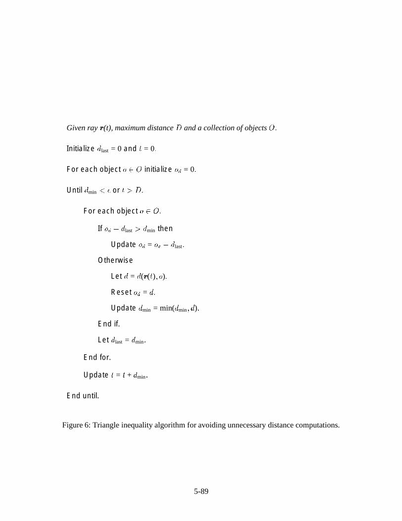
2.6.3 The Triangle Inequality
The triangle inequality,
��� � ��� �� � ��� � ��� �� + �� � ��� ���� � ��� ��� 3 � (19)
is part of the definition of any metric. It can also help eliminate unnecessary distance computations
for collections of objects. When computing the shortest distance between a point and a collection
5-86

Make a heap�
of bounding volume distances to each object.
Initialize
= � �Repeat
Let
be the lesser of
or the distance to the contents of the bounding volume
at the top of the heap.
Remove the top of the heap and re-heap.
Let
� be the distance to the bounding volume now at the top of the heap.
Until �
� or the heap is empty.
return �
Figure 5: An efficient algorithm for finding the closest object of a collection using bounding
volumes.
5-87

of objects, one need not compute the distance to objects whose last distance evaluation minus the
distance traversed along the ray since that last evaluation is still larger than the distance to the
currently closest object. The triangle inequality enhancement algorithm is outlined in Figure 6.
2.6.4 Octree Partitioning
Eliminating empty space certainly aids rendering efficiency, but the major benefit of partitioning
is that it allows the imposition of local bounds on the Lipschitz constants yielding tighter signed
distance bounds. Octree partitioning has been used in the polygonization [Bloomenthal, 1989]
and ray tracing [Kalra & Barr, 1989] of implicit surfaces. Sphere tracing reaps the same benefits
from spatial partitioning as did the root finding method in [Kalra & Barr, 1989], which used the
Lipschitz constant to cull octree nodes guaranteed not to intersect the implicit surface.
Ray intersection with an implicit surface defined by a signed distance bound is penalized by
the section of the domain where the gradient magnitude is greatest. Chopping an object into the
union of smaller chunks allows each chunk to be treated individually, penalized only by the largest
gradient within its bounds. Since the partitioning algorithm in [Kalra & Barr, 1989] required only
a bound on the Lipschitz constant of the function, the use of this octree in no way restricts the
domain of functions available for sphere tracing.
Octree partitioning further enhances sphere tracing of unions and lists by optionally storing an
index to the object closest to the cell. An object is closest to an octree cell if and only if it is the
closest object to every point in the cell. Under this definition, some cells may not have a closest
object. By the triangle inequality (19), an object is closest to a cell if the distance from the cell’s
centroid to the object, plus the distance from the centroid to the cell corner, is still less than the
distance from the centroid to any other object.
2.6.5 Convexity
Convexity can be defined in any number of ways. For example, metric topology [Kaplansky, 1977]
defines a set in a complete metric space as convex if and only if for any two distinct points in the
set, there exists a third distinct point whose distance from the first two points sums to their distance
5-88
Given ray � (t), maximum distance�
and a collection of objects� �
Initialize
last = 0 and�
= 0 �For each object �
�initialize � � = 0 �
Until
min� � or
��� � �For each object �
� �If � � � last
� min then
Update � � = � � � last�
Otherwise
Let
= ( � ( � ) � � ) �
Reset � � = �
Update
min = min(
min� ) �
End if.
Let
last =
min�
End for.
Update�
=�
+
min�
End until.
Figure 6: Triangle inequality algorithm for avoiding unnecessary distance computations.
5-89

from each other. The coordinate space 3 allows the more familiar definition of convexity.
Definition 4 [Farin, 1990] A set� � 3 is convex if and only if the line segment
lerp(� ��� ) = �
�+ (1 ��� ) � � � � [0 � 1] (20)
connecting the two endpoints� � � � is a subset of
� �Knowing that an object is convex can make sphere tracing more efficient by increasing the
step size along the ray.
Theorem 4 Let� � 3 be a convex set defined implicitly by the signed distance function � � Then
given a unit vector � 3 the line segment
lerp(� � � (
�)� ��� � � (
�)� ) (21)
does not intersect�
except possibly at its second endpoint.
Proof: The gradient of a signed distance function� � has the following properties on the
complement of a convex set 3 � � : (1) it is continuous; (2) its magnitude is one (the change in
the function equals the change in the distance); and (3) its direction points directly away from the
closest point on the implicit surface. Hence, for any�� 3 � � we know the closest point in A,
and its surface normal points toward� � Since
�is convex, it cannot penetrate the tangent plane to� �
The intersection of a ray anchored at�
and direction � with the tangent plane normal to the
vector� � (
�) a distance of � (
�) from
�is given by the second endpoint of (21).
�
Corollary 4.1 If� � (
�) ��� � 0 then the ray anchored at
�and direction � does not intersect the
implicit surface of � �Theorem 4 allows sphere tracing to make larger steps toward convex objects, and Corollary 4.1
allows sphere tracing to avoid computing the distance to convex objects it has stepped beyond.
The convexity enhancement likely causes sphere tracing to converge quadratically, because of its
similarity to Newton’s method, which also converges quadratically.
5-90

Bounding volumes are usually convex, and combining these two techniques can further reduce
the computation of unnecessary distances.
Knowledge of convexity becomes a necessity for rendering scenes with a horizon line. Consider
a ground plane and a ray parallel to it. Sphere tracing will step along this ray at fixed intervals
looking for an intersection that never happens. Corollary 4.1 avoids this situation whereas
Theorem 4 hastens convergence of rays nearly parallel to the ground plane.
3 Antialiasing
Tracing cones instead of rays resulted in an area-sampling antialiasing method in [Amanatides,
1984]. Cone tracing computed the intersection of cones with spheres, planes and polygons to
symbolically prefilter an image, eliminating the aliasing artifacts that result from point sampling.
Sphere tracing is easily coerced into detecting and approximating cone intersections with any
implicit surface defined by a signed distance function. One must still implement the details of
the cone tracing algorithm to determine the shape of the cones as they bounce around a scene,
but may rely on unbounding spheres to increase the efficiency of determining cone intersections.
Moreover, sphere tracing only enhances the detection of cone intersections at silhouette edges, and
is of no help in the other forms of aliasing cone tracing also fixes, such as texture aliasing.
At some point along a grazing ray, the sequence of unbounding spheres shrinks, falling within
the bounds of the cone, then enlarges, escaping the bounds of the cone. This poses the problem
of ‘‘choosing a representative’’ [Amanatides, 1984] --- a location to take a sample to approximate
the shading of the cone’s intersection with the surface.
A cover is a pixel-radius offset bounding an implicit surface on the inside and outside such
that a ray-cover intersection indicates a cone-object intersection [Thomas et al, 1989]. Given an
implicit surface defined by the signed distance function � (�
) � its outer cover is the global offset
surface implicitly defined by � (�
) �� � and its inner cover is the global offset surface implicitly
defined by � (�
) + � �� where � � is the radius of a pixel (one-half of the diameter of a pixel [Hart &
DeFanti, 1991]). In other words, the outer cover is the surface ��� 1( � � ) and the inner cover is the
5-91

surface �� 1( � � ) � Instead of sphere tracing the implicit surface of � (�
) � the antialiasing algorithm
sphere traces the inner cover --- the implicit surface of � (�
) + � � �The development of covers proposes the most representative choice for silhouette antialiasing
would be the point along the section of the ray closest to the surface. Hence, of the unbounding
spheres inside the cone, the center of the smallest sphere (with respect to pixel size) becomes the
representative sample. Though this sample is off the implicit surface, one assumes a reasonable
level of continuity in the gradient of the distance function to define a usable surface normal. The
sequence along the ray of unbounding spheres are related to a cone as shown in Figure 7.
cone boundary
ray
cone intersection
representative
inne
r cov
er
surfa
ceouter
cove
r
Figure 7: Sphere tracing approximates cone intersection. The ray intersects the original surface
but misses its inner cover. This cone intersection will account for more than half of the pixel’s
illumination.
For smooth implicit surfaces, one may assume local planarity. Hence the implicit surface is
assumed to cover the cross section of the cone with a straight edge of the given distance from the
cone’s center. The amount of influence this shaded point has, with respect to the points the ray
intersects further on, depends on the signed distance function evaluated at the representative � (�
)
(the radius of the closest unbounding sphere) to the implicit surface. The fraction of coverage of a
disk of radius � � by an intersecting half-plane of signed distance � (�
) from its center is given by
� =12� � (
�) � � 2
�� � (
�)2
�� 2
�
� 1�
arcsin� (
�)
� �
(22)
and is derived in [Thompson, 1990]. Ray traversal proceeds in steps of � (�
) + � � (which may take it
through the surface). The percentage of coverage � represents the cone intersection of the grazing
5-92

ray. It is treated as an opacity and is accumulated and used to blend the shading of the current
representative�
with the shading resulting from further near misses and intersections, using the
standard rules of image compositing [Porter & Duff, 1984].
For intersection edges, one must keep track of all signed distance functions whose unbounding
spheres fit within the bounds of the cone. Upon ray intersection approximation, the signed distance
functions of each of the intersecting surfaces provide the proportions for the proper combination
of their shading properties. The representative for intersection is the last point of the ray traversal
sequence, the point that satisfies the convergence test.
Often the signed distance function is too expensive to compute efficiently and a signed distance
bound is used. A bound may return unbounding spheres whose radii prematurely shrink below
the radius of a pixel, resulting in incorrect cone intersections. In this case, a separate distance
approximation may be useful. For example, [Pratt, 1987; Taubin, 1994] estimate the distance to the
implicit surface of � with the first order approximation ��� �� � � ��� � In general, this approximation is
not necessarily a distance bound. Lemma 1 of [Taubin, 1994] asserts that this approximation is
asymptotic to geometric distance as one approaches the surface. Cone intersections can hence be
more accurately determined by this approximation than by the signed distance bound.
For texture aliasing, cone tracing filtered the texture based on the radius of the cone at
intersection. Since cone tracing is maintained within the unbounding-sphere ray-intersection
scheme, textures can be likewise antialiased within this rendering system.
4 Results
Sphere tracing simplifies the implementation of an implicit surface ray tracer, and runs at speeds
comparable to other implicit surface rendering algorithms.
4.1 Implementation
Sphere tracing has been implemented in a rendering system called zeno. Inclusion of an implicit
surface into zeno requires the definition of two functions: a signed distance function for ray
5-93

intersection, and a surface normal function for shading.
A new primitive or operation can be incorporated into zeno with no more than a distance
bound. The negative part of the signed distance bound is only necessary for some constructive
solid geometry and blending operations, and is not needed for the visualization of functions that
are zero-valued inside the implicit surface. The surface normal function can be avoided by using a
general six-sample numerical gradient approximation of the distance bound gradient. Since most
of the time is spent on ray intersection, the inefficient numerical gradient approximation has a
negligible impact on rendering performance.
The simplicity with which implicit surfaces are incorporated in zeno makes it useful for
visualization of mathematical tasks and investigation of new implicit surfaces. For example, a
homotopy that removes a 720 � twist from a ribbon without moving either end formed the basis
for the animated short ‘‘Air on the Dirac Strings’’ [Sandin et al, 1993], for which zeno rendered
a segment. This homotopy is based heavily on interpolated quaternion rotations and was easily
incorporated into zeno as a domain transformation after a quick search and analysis of the most
extreme deformation in the homotopy [Hart et al, 1993].
4.2 Exhibition
The three tori in Figure 8 are combined using the superelliptic blend described in Appendix D.2.
The tori all are of major radius one, and minor radius one-tenth. The blue-green blend is quadratic
extending along the tori a radius of 0 � 5 from their intersection. The red-green blend also has radius
0 � 5 but is degree eight. The red-blue blend is also degree eight but has a radius of only 0 � 2 �Sphere tracing rendered Figure 8 (left) in 12:47 at a resolution of only 256 � 256 using
prefiltering to avoid the severe aliasing that ordinarily accompany such low sampling rates.
Experiments on the difference of execution using point sampling and area sampling show that the
increased execution time due to area sampling is negligible.
Although the superelliptic blend is implemented in zeno as a signed distance bound, it returns
an underestimated distance of no less than 70% of the actual distance which adequately indicated
cone intersections, as the enlargement demonstrates in Figure 8 (upper right).
5-94
Figure 8: Three blends of tori (left), blowup (upper right) and work image (lower right).
5-95

The work image in Figure 8 (lower right) shows that sphere tracing concentrates on silhouette
edges. Blue areas converge from 10 iterations, green around 50 and red over 100.
Figure 9: A logo for zeno.
Figure 9 demonstrates a generalized cylinder, from Appendix C, whose skeleton consists of a
space curve modeled with 14 Bezier control polygons. Sphere tracing can render this scene in as
fast as 5:30 using bounding spheres to eliminate unnecessary distance computations. The curved
horizon is an artifact of the yonder clipping sphere of radius 1 � 000 used to terminate ray stepping.
Figure 10 demonstrates the robustness of sphere tracing on creased surfaces. Both images were
rendered with prefiltering at a resolution of 512 � 512 � and in 16:48 for the cylinders, 12:36 for
the cube.
The creases were created as CSG unions and intersections, defined implicitly by the continuous
but non-differentiable minimum and maximum operations from Section 2.5. The resulting edge
was then merged into a third object using the pseudonorm blend from Appendix D.2. Such creased
surfaces appear periodically in a variety of shapes, particularly in the modeling of biological forms.
Figure 11 illustrates the ‘‘noise’’ range deformation described in Appendix F. The left image
uses a single octave of noise, whereas the next two use six octaves, whose amplitude was scaled
5-96

Figure 10: Creases created by blended edges.
Figure 11: ‘‘Lava’’ (left) modeled as a sphere deformed by the noise function. ‘‘Muscle’’ (center)
modeled with Brownian 1 � � 2 noise. ‘‘Rock’’ (right) modeled with fractional Brownian 1 � � noise.
5-97

by 1 � � 2 and 1 � � � respectively, yielding a muscle texture and a rocky surface. The three images
were each rendered at a resolution of 256 � 256 in (from left to right) approximately five minutes,
half-an-hour, and two hours. The high variation of distance estimates prohibited prefiltering the
results of the noise function.
4.3 Analysis
Sphere tracing convergence is entirely linear whereas other general root finders, such as interval
analysis, have a linearly-convergent root isolation phase followed by a quadratically-convergent
root refinement stage. Work images, such as Figure 8 (lower right), show that ray intersection
is most costly at silhouette edges. When sphere tracing these edges, the distance to the surface
is only a fraction of the distance to the ray intersection which slows convergence. For other
methods like interval analysis, silhouettes are double roots (that prevent root refinement) and their
neighborhoods consist of closely-spaced pairs of roots. Such root pairs are costly for midpoint
subdivision root refinement methods to separate since the distance between the two roots can be
several orders of magnitude smaller than the initial interval.
The convexity enhancement hastened convergence by 31% as shown in Table 2. With more
primitives, this same table shows the triangle inequality enhancement to more than double the
convergence rate, and when combined with convexity, enhances ordinary sphere tracing by 60%.
Table 2 also compares various enhanced rendering times for the zeno logo. The fact that
all 14 Bezier curves were nearly equidistant from the eye prevented the triangle inequality from
significantly reducing unnecessary distance evaluations until sphere tracing had traversed much of
each ray.
Figure 12 reveals the distribution of step sizes used in sphere tracing a ball. This histogram
counted only the distance evaluations used to intersect primary (eye) rays.
Unimproved sphere tracing is evenly distributed, with a small hump in the middle. An octree
replaces the increased distance computation in this humped area with octree parsing overhead,
(which this histogram does not measure). Echoes of the octree bounds cause the oscillations
at the high end of its spectrum, whereas the low end adheres to the unenhanced performance.
5-98

scene execution time relative time enhancement
single sphere 2:00 100% none
1:23 69% convexity
9 spheres/plane 2:53 100% none
1:42 59% convexity
1:19 46% triangle inequality
1:10 40% both
zeno logo 26:29 100% none
19:23 73% triangle inequality
5:28 21% bounding spheres
‘‘Lava’’ 4:37 1 (single noise)
‘‘Muscle’’ 33:52 7.3 (1 � � 2 noise)
‘‘Rock’’ 2:06:56 27.5 (1 � � noise)
Table 2: Comparison of execution times for enhanced sphere tracing of various scenes.
5-99

1
10
100
1000
10000
100000
1e-05 0.0001 0.001 0.01 0.1 1 10 100 1000
# of
Ste
ps
Step Size
UnenhancedOctree
Convex
Figure 12: Histogram of step sizes for sphere tracing a ball.
5-100

Experiments on simple scenes failed to demonstrate any increased performance from the octree
enhancement, although more complicated scenes are likely to benefit from its use.
The convex histogram demonstrates the power of this enhancement. Its slope on the left
confirms the expectation from Section 2.6.5 that it provides sphere tracing a faster order of
convergence. The right side of this histogram is significantly reduced, due to the cessation of
stepping after moving beyond the sphere.
The spike in the unenhanced and convex graphs indicates the distance from the eye to the
ball, which is the first step taken by every ray emanating from the eye-point. One can remove
these spikes from the graph by measuring this distance once and refer to it as the first step for
rays emanating from the eye-point, and likewise for the light sources. This ‘‘head start’’ barely
improved performance in experiments.
Similar histograms in [Zuiderveld et al, 1992] measured performance logarithmically in the
number of steps but linearly in step size. As a result, their graphs were more logarithmically shaped
than Figure 12.
The accuracy of the distance estimate is directly proportionate to the rate of convergence.
Experiments on a sphere show that half the distance doubles the number of steps. The step-size
histograms in Figure 13 reveals the effects of distance underestimation.
The relationship between distance accuracy and sphere tracing performance suggests that
in certain cases a slower signed distance function may perform better than a fast distance
underestimate. For example, consider the distance to an ellipsoid with major axes of radius 100,
100 and 1 modeled as a non-uniform scale transformation of the unit sphere. Section E yields
a signed distance bound which returns at best the distance to the ellipsoid, and at worst 1% of
the distance, in closed form, whereas [Hart, 1994] yields a signed distance function which returns
the exact distance at the expense of several Newton iterations. In this case, the signed distance
function would likely result in better performance.
Finally, the Lipschitz constants of the noise functions are 3 for single noise, 6 for 1 � � 2 noise
and 18 for 1 � � noise (six octaves). The timings in Table 2 corresponding to the images in Figure 11
show that the 1 � � 2-noise rendering time was actually 7 � 3 times (instead of the expected value of
5-101

1000
10000
100000
1e+06
1e-05 0.0001 0.001 0.01 0.1 1 10 100 1000
# of
Ste
ps
Step Size
Full distanceHalf distance
Quarter distance
Figure 13: Halving step sizes doubles convergence time.
5-102

twice) the single noise time. The likely reason is that the 1 � � 2 noise invokes the noise function six
times more than the single noise function (yielding an expected value of 12 times). The 1 � � -noise
rendering time was 27 � 5 times longer than that of single noise (less than the expected 36 times),
and 3 � 75 times longer than the 1 � � 2 noise (slightly larger than the expected value of 3).
5 Conclusion
Sphere tracing provides a tool for investigating a larger variety of implicit surfaces than before
possible.
With its enhancements and prefiltering, sphere tracing becomes a competitive presentation-
quality implicit surface renderer. In particular, the convexity enhancement greatly increases
rendering speeds, and the triangle inequality is quite effective for large assortments of objects.
Bounding volumes also increase rendering performance as expected. However, techniques based
on image coherence and space coherence (octree) did not perform as well.
Whereas sphere tracing performed significantly slower than standard ray tracing on simple
objects consisting of quadrics and polygons, it excelled at rendering the results of sophisticated
geometric modeling operations.
The geometric nature of sphere tracing adapts it to symbolic prefiltering, supporting antialiasing
at a nominal overhead.
In lieu of direct experimental comparison, several theoretical arguments show sphere tracing
as a viable alternative to interval analysis and L-G surfaces.
5.1 Further Research
Sphere tracing demonstrates the utility of signed distance functions in the task of rendering
geometric implicit surfaces. We expect these functions will similarly enhance other applications,
particularly in the area of geometric processing. As geometric distance becomes more important
in computer-aided geometric design and other areas of modeling, the demand for more efficient
geometric distance algorithms will increase.
5-103

In retrospect, the use of the Euclidean distance metric seems an arbitrary choice for sphere
tracing. The linear nature of the chessboard and Manhatten metrics may result in more efficiently
computed distances and ray intersection. ‘‘Cube-tracing’’ and ‘‘octahedron-tracing’’ algorithms
are left as further research.
5.2 Acknowledgements
Thanks to Tom DeFanti and Larry Smarr for their support of the first year of this research, and
to Pat Flynn, Robert Bamberger and Tom Fischer for welcoming me and my research into the
Imaging Research Laboratory at WSU.
This research is supported by the National Science Foundation under grant CCR-9309210. Any
opinions, findings, conclusions or recommendations expressed in this manuscript are those of the
author and do not necessarily reflect the view of the National Science Foundation.
Special thanks to Alan Norton who, in 1989, encouraged me to apply sphere tracing to
non-fractal models. The task of tracking down and deriving the distances in the appendix was
greatly helped by conversations with Al Barr, Chandrajit Bajaj, Charlie Gunn, Pat Hanrahan, Jim
Kajiya, Don Mitchell and Alyn Rockwood.
Brian Wyvill and Jules Bloomenthal deserve special mention for inspiring this research by
putting together an excellent course on implicit surfaces at SIGGRAPH ’90.
References
[Agin & Binford, 1976] Agin, G. J. and Binford, T. O. Computer description of curved objects.
IEEE Transactions on Computers C-25(4), Apr. 1976, pp. 439--449.
[Amanatides, 1984] Amanatides, J. Ray tracing with cones. Computer Graphics 18(3), July 1984,
pp. 129--135.
[Ballard & Brown, 1982] Ballard, D. H. and Brown, C. M. Computer Vision. Prentice-Hall,
Englewood Cliffs, NJ, 1982.
5-104

[Barnhill et al, 1992] Barnhill, R. E., Frost, T. M., and Kersey, S. N. Self-intersections and offset
surfaces. In Barnhill, R. E., ed., Geometry Processing for Design and Manufacture, pp. 35--44.
SIAM, 1992.
[Barr, 1981] Barr, A. H. Superquadrics and angle-preserving transformations. IEEE Computer
Graphics and Applications 1(1), 1981, pp. 11--23.
[Barr, 1984] Barr, A. H. Global and local deformations of solid primitives. Computer Graphics
18(3), July 1984, pp. 21--30.
[Blinn, 1982] Blinn, J. F. A generalization of algebraic surface drawing. ACM Transactions on
Graphics 1(3), July 1982, pp. 235--256.
[Bloomenthal & Shoemake, 1991] Bloomenthal, J. and Shoemake, K. Convolution surfaces.
Computer Graphics 25(4), July 1991, pp. 251--256.
[Bloomenthal, 1988] Bloomenthal, J. Polygonization of implicit surfaces. Computer Aided
Geometric Design 5(4), Nov. 1988, pp. 341--355.
[Bloomenthal, 1989] Bloomenthal, J. Techniques for implicit modeling. Technical Report
P89-00106, Xerox PARC, 1989. Appears in SIGGRAPH ’93 Course Notes #25 ‘‘Design,
Visualization and Animation of Implicit Surfaces’’.
[Bronsvoort & Klok, 1985] Bronsvoort, W. F. and Klok, F. Ray tracing generalized cylinders.
ACM Transactions on Graphics 4(4), Oct. 1985, pp. 291--303.
[Farin, 1990] Farin, G. E. Curves and Surfaces for Computer-Aided Geometric Design. Academic
Press, San Diego, 1990.
[Gerald & Wheatley, 1989] Gerald, C. F. and Wheatley, P. O. Applied Numerical Analysis.
Addison-Wesley, Reading, MA, 1989.
[Goldman, 1983] Goldman, R. N. Two approaches to a computer model for quadric surfaces.
IEEE Computer Graphics and Applications 3(5), Sept. 1983, pp. 21--24.
5-105

[Hanrahan, 1983] Hanrahan, P. Ray tracing algebraic surfaces. Computer Graphics 17(3), 1983,
pp. 83--90.
[Hart & DeFanti, 1991] Hart, J. C. and DeFanti, T. A. Efficient antialiased rendering of 3-D linear
fractals. Computer Graphics 25(3), 1991.
[Hart et al, 1989] Hart, J. C., Sandin, D. J., and Kauffman, L. H. Ray tracing deterministic 3-D
fractals. Computer Graphics 23(3), 1989, pp. 289--296.
[Hart et al, 1993] Hart, J. C., Francis, G. K., and Kauffman, L. H. Visualizing quaternion rotation.
Manuscript, in review, 1993.
[Hart, 1994] Hart, J. C. Distance to an ellipsoid. In Heckbert, P., ed., Graphics Gems IV, pp.
113--119. Academic Press, 1994.
[Hoffman, 1989] Hoffman, C. M. Geometric and Solid Modeling. Morgan Kaufmann, 1989.
[Kalra & Barr, 1989] Kalra, D. and Barr, A. H. Guaranteed ray intersections with implicit surfaces.
Computer Graphics 23(3), July 1989, pp. 297--306.
[Kaplansky, 1977] Kaplansky, I. Set Theory and Metric Spaces. Chelsea, New York, 1977.
[Kay & Kajiya, 1986] Kay, T. L. and Kajiya, J. T. Ray tracing complex scenes. Computer
Graphics 20(4), 1986, pp. 269--278.
[Lewis, 1989] Lewis, J. P. Algorithms for solid noise synthesis. Computer Graphics 23(3), July
1989, pp. 263--270.
[Mitchell & Hanrahan, 1992] Mitchell, D. and Hanrahan, P. Illumination from curved reflectors.
Computer Graphics 26(2), July 1992, pp. 283--291.
[Mitchell, 1990a] Mitchell, D. P. The antialiasing problem in ray tracing. In Advanced Topics in
Ray Tracing. SIGGRAPH ’90 Course Notes, Aug. 1990.
5-106

[Mitchell, 1990b] Mitchell, D. P. Robust ray intersection with interval arithmetic. In Proc. of
Graphics Interface ’90. Morgan Kauffman, 1990, pp. 68--74.
[Nishimura et al, 1985] Nishimura, H., Hirai, M., Kawai, T., Kawata, T., Shirakawa, I., and
Omura, K. Object modeling by distribution function and a method of image generation. In
Proc. of Electronics Communication Conference ’85, 1985, pp. 718--725. (Japanese).
[Perlin & Hoffert, 1989] Perlin, K. and Hoffert, E. M. Hypertexture. Computer Graphics 23(3),
July 1989, pp. 253--262.
[Porter & Duff, 1984] Porter, T. and Duff, T. Compositing digital images. Computer Graphics
18(3), 1984, pp. 253--259.
[Pratt, 1987] Pratt, V. Direct least-squares fitting of algebraic surfaces. Computer Graphics 21(4),
July 1987, pp. 145--152.
[Ricci, 1974] Ricci, A. A constructive geometry for computer graphics. Computer Journal 16(2),
May 1974, pp. 157--160.
[Rockwood & Owen, 1987] Rockwood, A. P. and Owen, J. C. Blending surfaces in solid
modeling. In Farin, G., ed., Geometric Modelling, pp. 367--383. SIAM, 1987.
[Rockwood, 1989] Rockwood, A. P. The displacement method for implicit blending surfaces in
solid models. ACM Transactions on Graphics 8(4), Oct. 1989, pp. 279--297.
[Roth, 1982] Roth, S. D. Ray casting for modeling solids. Computer Graphics and Image
Processing 18(2), February 1982, pp. 109--144.
[Sandin et al, 1993] Sandin, D. J., Kauffman, L. H., and Francis, G. K. Air on the Dirac strings.
SIGGRAPH Video Review 93, 1993. (Animation).
[Schneider, 1990] Schneider, P. J. Solving the nearest-point-on-curve problem. In Glassner, A. S.,
ed., Graphics Gems (I), pp. 607--611. Academic Press, Boston, 1990.
5-107

[Sederberg & Zundel, 1989] Sederberg, T. W. and Zundel, A. K. Scan line display of algebraic
surfaces. Computer Graphics 23(3), July 1989, pp. 147--156.
[Snyder, 1992] Snyder, J. M. Interval analysis for computer graphics. Computer Graphics 26(2),
July 1992, pp. 121--130.
[Stander & Hart, 1994] Stander, B. T. and Hart, J. C. A Lipschitz method for accelerated volume
rendering. In Proc. of Volume Visualization Symposium ’94, Oct. 1994. To appear.
[Taubin, 1994] Taubin, G. Distance approximations for rasterizing implicit curves. ACM Trans-
actions on Graphics 13(1), Jan. 1994, pp. 3--42.
[Thomas et al, 1989] Thomas, D., Netravali, A. N., and Fox, D. S. Antialiased ray tracing with
covers. Computer Graphics Forum 8(4), December 1989, pp. 325--336.
[Thompson, 1990] Thompson, K. Area of intersection: Circle and a half-plane. In Glassner, A. S.,
ed., Graphics Gems, pp. 38--39. Academic Press, Boston, 1990.
[van Wijk, 1984] van Wijk, J. Ray tracing objects defined by sweeping a sphere. In Proc. of
Eurographics ’84. Elsevier, 1984, pp. 73--82.
[Von Herzen & Barr, 1987] Von Herzen, B. and Barr, A. H. Accurate triangulations of deformed,
intersecting surfaces. Computer Graphics 21(4), July 1987, pp. 103--110.
[Von Herzen et al, 1990] Von Herzen, B., Barr, A. H., and Zatz, H. R. Geometric collisions for
time-dependent parameteric surfaces. Computer Graphics 24(4), Aug. 1990, pp. 39--48.
[Voss, 1988] Voss, R. F. Fractals in nature: From characterization to simulation. In Peitgen, H.
and Saupe, D., eds., The Science of Fractal Images, pp. 21--70. Springer-Verlag, New York,
1988.
[Wyvill & Trotman, 1990] Wyvill, G. and Trotman, A. Ray tracing soft objects. In Proc. of
Computer Graphics International ’90. Springer Verlag, 1990.
5-108

[Wyvill et al, 1986] Wyvill, G., McPheeters, C., and Wyvill, B. Data structure for soft objects.
Visual Computer 2(4), 1986, pp. 227--234.
[Zuiderveld et al, 1992] Zuiderveld, K. J., Koning, A. H. J., and Viergever, M. A. Acceleration of
ray-casting using 3-D distance transforms. In Proc. of Visualization in Biomedical Computing
1992, vol. 1808, Oct. 1992, pp. 324--335.
A Distance to Natural Quadrics and Torus
These appendices derive signed distance functions, bounds and Lipschitz constants and bounds
for a variety of primitives and operations in the hope that they will aid in the implementation of
sphere tracing, while also serving as a tutorial in developing signed distance functions, bounds and
Lipschitz constants and bounds for other primitives and operations.
Distances to the standard solid modeling primitives are listed below. The geometric rendering
algorithm is not as efficient compared to the standard closed-form solutions. Instead, these
distances are useful when the primitives are used in higher-order constructions such as blends and
deformations.
Plane The signed distance to a plane�
with unit normal � intersecting the point ��� is
(� � � ) =
���� �
� � (23)
Sphere A sphere is defined as the locus of points a fixed distance from given point. The distance
to the unit sphere � about at the origin hence given by
(� � � ) =
�� ����� � 1 � (24)
Through domain transformations (Section E, the radius and location of the sphere may be
changed. The sphere may even become an ellipsoid, though this reformulates the signed distance
function into one requiring the solution to a sixth-degree polynomial [Hart, 1994]. Through
alternate distance metrics (Section B), the sphere can become a superellipsoid. These techniques
also generalize the rest of the basic primitives as well.
5-109

Cylinder The distance to a unit-radius cylinder centered about the � -axis is found by projecting
into the � � -plane and measuring the distance to the unit circle
(� � � ��� ) =
���( �� � )
��� � 1 � (25)
Note that in (25), and throughout the rest of the appendix,�
= ( �� � � � ) �Cone The distance to a cone centered at the origin oriented along the � -axis is
(� � � ��� � ) =
���( �� � )
���cos � � � � � sin � � (26)
where � is the angle of divergence from the � -axis. The trigonometry behind its derivation is
illustrated by Figure 14.
���( � � � )
�� � � � � tan �( �� � � � )�
�
� � � tan � � � �� � (�� )
� � cos� � ��� � sin
�
Figure 14: Geometry for distance to a cone.
Torus The torus is the product of two circles, and its distance is evaluated as such
(� ��� ) =
���(���( � � � )
�� ��� � � )��� �
� (27)
for a torus of major radius � and minor radius � � centered at the origin and spun about the � -axis.
5-110

B Distance to Superquadrics
Superquadrics [Barr, 1981] result from the generalization of distance metrics. Distance to the basic
primitives all used the�����
operator. In two dimensions, this operator generalizes to the � -norm
���( �� � )
��� �
= (� � � �
+� � � �
)1� (28)
which, when � = 2 � becomes the familiar Euclidean metric whose circle is a round circle. The
Manhattan metric (� = 1) has a diamond for its circle. Taking the limit as � � � results in the
chessboard metric ��( �� � )
��� �= max �� � (29)
where a square forms its circle. The other intervening values for � produce rounded variations
on these basic shapes, and setting 0 � � � 1 produces pinched versions. Generalized spheres,
so-called superellipsoids, are produced by a ��� -norm as
���( �� � � � )
��� ���=
���(��( �� � )
��� � � � )��� � � (30)
The natural quadrics now generalize to superquadrics, and tori likewise become supertori,
whose distances are measured in the appropriate metric. One unifying metric space must be used
for the distances to be comparable. Hence, ��� -norm distances must be converted into Euclidean
distances.
Let � (�
) return a ��� -norm distance to its implicit surface. This distance defines the radius of
an unbounding superellipsoid. The radius of the largest Euclidean sphere �� inscribed within the��� -norm superellipsoid of radius �� (in the ��� -norm metric) is given by
� � =
� � � � � �� ( � 33� � 3
3� � 3
3 )�� ���
if � � 2
� otherwise(31)
C Distance to Offset Surfaces
Given some closed skeleton geometry � � 3 � then the global offset surface is defined geometri-
cally by the implicit equation (� � � ) � � = 0 � (32)
5-111

When � is constant, the resulting implicit surface fleshes out the skeleton � �The point-to-set distance is defined as a search through the entire set for the closest point. If � �
has a surface normal defined everywhere, then the point � in � closest to�
is one of the points on
� � whose normal extends directly toward� � This greatly reduces the search space for point-to-set
distance determination to some primitives, such as parametric surfaces.
This formulation of the point-to-set distance can cause problems when used to define an offset,
however. If the skeleton is a generator surface represented by the parametric function � ( � ��� ) � then
the local offset surface is defined by the parametric function
� ( � ��� ) = � ( � ��� ) + ��� ( � ��� ) (33)
where
� ( � ��� ) =��� ( � ��� )��� � � ( � ��� )
�� � �� ( � ��� )��� � � ( � ��� )�� (34)
is the unit-length surface normal at � ( � ��� ) and �� � ��� are the partial derivatives with respect to � ��� �Global offsets are usually defined as geometric implicit surfaces whereas local offsets are
usually defined parametrically. Global offsets are the more desirable representation [Hoffman,
1989], and in particular avoid interior surfaces which can cause problems in ray-tracing and CSG
[van Wijk, 1984].
The offset of an algebraic implicit surface is algebraic, though of higher degree in general.
Likewise, parametric versions of the offset surface are typically of higher degree than the
generator. This increase in degree is due, in part, to the use of distance (requiring a cross
product and square root in (34)) in the definition of offset surfaces. Several techniques have
been developed to approximate offset surfaces with lower-degree representations. Treating offset
surfaces geometrically overcomes the problems of dealing with unnecessarily high degree algebraic
representations and loss of precision due to inexact low-degree approximations.
One useful skeletal model is the simplified generalized cylinder, which is a global offset surface
defined as the locus of points a fixed distance from a space curve piecewise defined by 3-D Bezier
curves.
Define the space curve parametrically as the image of the function � : � 3 � Without loss
of generality, assume the point we want to find the distance from the space curve is the origin.
5-112

Then the closest point on the space curve will be either of the endpoints, or a point on the space
curve whose tangent is perpendicular with a vector pointing to the origin. The latter are found by
solving� ( � ) � � � ( � ) = 0 � (35)
Let � be a cubic Bezier curve. Then [Schneider, 1990] shows how (35) can be converted into a
degree-five 1-D Bezier curve, a Bernstein polynomial whose graph is bounded by the convex hull
of the control points. Bernstein polynomials can be solved efficiently using a technique described
in [Rockwood & Owen, 1987].
Generalized cylinders are demonstrated in Figure 9 in Section 4.2.
D Distance to Blended Objects
A blend is a smoothing of the joint where sections of an object meet. The following two blends
are local, meaning that they affect only a portion of the object. This is useful in computer-aided
geometric design so that blends on different parts of an object do not interfere, and is useful in
computer graphics to bound and cull blends from rendering when possible.
D.1 Soft Metablobbies
[Blinn, 1982] used a Gaussian distribution function to produce a blending function which has
come to be known as the ‘‘blobby’’ model. ‘‘Soft’’ objects approximate Gaussian distribution
with a sixth-degree polynomial to avoid exponentiation and localize the blends [Wyvill et al,
1986]. ‘‘Metaballs’’ approximate Gaussian distributions with piecewise quadratics to avoid
exponentiation and iterative root-finding [Nishimura et al, 1985].
Following [Wyvill et al, 1986], the following piecewise cubic in distance �
�� ( � ) =
� � � 2� 3
�3� 3
� 2�
2 + 1 if �� � �
0 otherwise.(36)
5-113

approximates a Gaussian distribution. A similar sixth-degree algebraic version also exists and is
typically used instead, avoiding distance computations at the expense of the higher degree [Wyvill
& Trotman, 1990].
Reformulating this function to accommodate the implicit surface definitions in this paper, (36)
forms the basis for a soft implicit surface consisting of � key points � � with radii � � � and threshold� � defined by the function
� (�
) = � � ���=1
���� ( �� � � � � ��� ) (37)
Negative keypoints are incorporated into the model by negating the value returned by�
��� () �Theorem 5 The distance to the implicit blend
�defined by (37) is bounded by
(� � � ) � 2
3� (
�)���=1
� � � (38)
Proof: Repeated differentiation of (36) produces
� �( � ) = 6
� 2
� 3� 6
�� 2
(39)
� ���( � ) = 12
�� 3
� 6� 2
� (40)
Solving� ���
( � ) = 0 yields the maximum slope, which occurs at the midpoint � = � � 2 � Its Lipschitz
constant is given by
Lip�
( � ) =� � �
( � � 2)�=
32 �
� (41)
The Lipschitz constant of a sum is bounded by the sum of the Lipschitz constants, which gives the
above result.�
In practice, local Lipschitz bounds may be used for tighter distance bounds by taking the first
summation in (38) over keypoints � with non-zero contributions. Additional efficiency results from
the use of bounding volumes of radius � �surrounding the keypoints � � � as detailed in [Wyvill &
Trotman, 1990].
D.2 Superelliptic Blends
The pseudonorm blend of [Rockwood & Owen, 1987] is a local blend. It returns the � -norm
distance to the blended union of implicit surfaces of signed distance functions. This blend is based
5-114

on the pioneering work of [Ricci, 1974], where implicit surfaces were defined by setting strictly
non-negative functions equal to one. Hence, we need to reformulate our functions into this style
by defining� � (
�) = max � 1 � � � (
�)
�� � 0 � (42)
and similarly for � � � The parameters �� � � � will delineate the extent of the local blends, in
Euclidean units if the components are signed distance functions. The pseudonorm blend of the
union of the implicit surface of � � with the implicit surface of � � is defined by the implicit surface
of
� � � ( � � (�
) � � � (�
)) =
� � � (�
) �� + � � (
�) � �
� � (�
) + � � (�
)(1 � � � (
�)
� � � � (�
)�
) � 1� � (43)
The parameter � is a thumbweight which describes how tightly the blend adheres to the original
surfaces. Conversely, the blended intersection is defined by � � � � ( � � � (�
) � � � � (�
)) �The domain of � � � is the area where � � (
�) � �
� and � � (�
) � � � � Outside this domain, it
is impossible to smoothly combine the results of � � and � � , resulting in a crease in the space
surrounding the blend [Rockwood & Owen, 1987]. Such gradient discontinuities can be disastrous
for some root finders, but do not impact the geometric ray intersection method described earlier.
The pseudonorm blend is demonstrated in Figures 8 and 10 in Section 4.2.
E Distances to Transformed Objects
Implicit surfaces are transformed by applying the inverse transformation to the space before
applying the function. Let � (�
) be a transformation and let � (�
) define the implicit surface. Then
the transformed implicit surface is defined as the implicit surface of
� ( � � 1(�
)) = 0 � (44)
The Lipschitz constant of the composition is no greater than the product of the component Lipschitz
constants. We are concerned with the Lipschitz constant of the transformation inverse, which is
not necessarily the inverse of the Lipschitz constant of the transformation.
5-115

Isometry Isometries are transformations that preserve distances. If�
is an isometry, the distance
returned by � needs no adjustment
(� � � � � � 1(0)) =
(� � 1(
�) � � � 1(0)) � (45)
Isometries include rotations, translations and reflections.
Uniform Scale A uniform scale is a transformation � (�
) of the form
� (�
) = ��
(46)
where � is the scale factor. The inverse � � 1 is a scale by 1 � � � Hence, the distance to a scaled
implicit surface is (� � � ( � � 1(0))) = �
( � � 1(
�) � � � 1(0)) (47)
and the Lipschitz constant of the inverse scale is 1 � � �Linear Deformation The distance to the linear image of an implicit surface is found by
determining the Lipschitz constant of the linear transformation’s inverse, which is also a linear
transformation.
The Lipschitz constant of an arbitrary linear transformation is found by the power method,
which iteratively finds the largest eigenvalue of a matrix [Gerald & Wheatley, 1989].
Taper The taper deformation scales two axes by a function � ( � ) of the third axis [Barr, 1984].
The taper is defined
taper (�
) = ( � ( � ) �� � ( � ) � � � ) (48)
whereas its inverse differs only by using � � 1( � ) instead of � ( � ) � The Lipschitz constant of the inverse
deformation is
Lip taper = min� ��� � � 1( � ) � (49)
In other words, the Lipschitz constant of the inverse taper is the amount of its ‘‘tightest’’ tapering.
5-116

Twist The twisting deformation rotates two axes by a linear function � ( � ) of the third axis.
Twisting is defined
twist (�
) =
�������� cos � ( � ) � � sin � ( � ) �� sin � ( � ) + � cos � ( � ) �
�
�������� (50)
whereas its inverse differs only by using � � 1( � ) instead of � ( � ) � Twisting is not Lipschitz on �since for any Lipschitz bound � one can find two points � at a great distance from the twisting
axis that are transformed farther apart by a ratio greater than � � Thus, twisting must be constrained
to a domain where it satisfies the Lipschitz criterion. One such domain is the unit cylinder oriented
along the twisting axis. The Lipschitz constant of the twist is computed from the worst case
scenario within the bounds of the unit cylinder as illustrated in Figure 15,
Lip twist = � 4 + � �
�� 2 � (51)
21
twist
� �
��� ��� Figure 15: Geometric calculation of the Lipschitz constant of the bounded twist deformation.
F Distance to Hypertextures
The use of sophisticated noise functions has greatly increased the power of procedural models for
making existing geometric representations more realistic. The recent work has applied stochastic
5-117

textures directly to the geometry instead of altering the shading [Perlin & Hoffert, 1989; Lewis,
1989].
The original ‘‘Hypertexture’’ system formulated implicit models for a variety of surface
phenomena, including hair and fire. This appendix focuses on incorporating hypertexture’s model
of noise into sphere tracing, though the same techniques can be used to adapt the other hypertexture
models as well.
‘‘Hypertexture’’ treats solid procedural noise as a deformation, and was designed for use
with implicit surfaces. Its original ray-tracing algorithm stepped along the ray in fixed intervals.
Determining a distance bound on a ‘‘hypertextured’’ shape allows sphere tracing to more efficiently
render its result.
Departing slightly from [Perlin & Hoffert, 1989], a noise function noise : 3 � deforms the
implicit surface of a signed distance function � by affecting its range (instead of its domain, as did
the previous appendix). The deformed surface is defined implicitly by the function � (�
) + noise(�
) �Band-limited solid noise results from the smooth interpolation of a lattice of random unit
vectors. Condensing [Perlin & Hoffert, 1989], the noise function is given by
noise( �� � � � ) =
� ���+1�
�=� ���
� � �+1�
�=� � �
��� �+1�
�=��� �
�1(� � � � � ) � 1(
� � �� � ) � 1(� � �� � )Γ( � ��� � ) � ( � � � � � �� � � �� ) (52)
where�
� is the cubic Gaussian approximation (36) used for soft objects, and Γ is an array of
random unit vectors. From Theorem 5, we know that Lip�
1 = 3 � 2 � Two opposing vectors can be
neighbors in à � so Lip à = 2 � Hence, their composition results in Lip noise = 3 �Fractal noise based on the 1 � ��� spectral distribution are formed by summing scaled versions
of the noise function
1 � � � noise(�
) =� � 1��=0
noise(2� �
)2 �
� � (53)
over � octaves [Perlin & Hoffert, 1989].
Setting the parameter � = 0 results in white noise, � = 1 in 1 � � noise typically found in nature
and � = 2 in Brownian motion. When in the range 1 ��� � 3 � its relationship to the fractal
dimension�
of the resulting surface it deforms is given by�
= 2+ 3 � �2 [Voss, 1988]. The 2
�factor
increases the frequency (contracts the graph horizontally) whereas the 1 � 2 ��
factor decreases the
5-118

amplitude (contracts the graph vertically).
For 1 � � noise, the amplitude decreases proportionately to the increase in frequency, so its
Lipschitz constant equals the sum of the individual noise functions,
Lip 1 � � noise = 3 � � (54)
Thus 1 � � noise is not Lipschitz, but its band-limited form for finite � is.
For Brownian motion ( � = 2), the amplitude decreases geometrically as the frequency increases,
resulting in
Lip 1 � � 2 noise = 3(2 � 1 � 2 � � 1) � 6 � (55)
Hence, Brownian motion is Lipschitz (which can also be derived from the definition of Brownian
motion as the integral of white noise).
The noise functions are demonstrated in Figure 11 in Section 4.2.
5-119