SPIDA 2012 – Part 7

Mixed Models with R: Generalized Linear Mixed Models

Georges Monette1 May 2012 Email: georges@yorku.ca http://scs.math.yorku.ca/index.php/SPIDA_2012

1 With thanks to many contributors: Ye Sun, Ernest Kwan, Gail Kunkel, Qing Shao, Alina Rivilis, Tammy Kostecki-Dillon, Pauline Wong, Yifaht Korman, Andrée Monette, Heather Krause, Hugh McCague, Yan Yan Wu and others 1

Generalized Linear Mixed Models (GLMMs) generalize Generalized Linear Models (GLMs) to Mixed Models as Linear Mixed Models (LMMs, HLMs) generalize Linear Models (LMs) to Mixed Models.

They allow modeling a non-normal response with a model that incorporates random effects.

However, the ratio of complexity GLMMGLM

is much greater than that of LMMLM

The reason is that integrating out the unseen random effects in the LMM is relatively easy thanks to the good behaviour of the normal distribution.

Except in a few special cases the random effects don't integrate out easily in GLMMs and various approximations need to be used. This is an active area of research and good practice is far from settled.

2

There are many functions in R that can be used for GLMMs. Some key ones:

Function Approach glmmPQL in MASS, nlme

A marriage of glm and lme using Penalized Quasi Likelihood: easy to use with familiar syntax of glm and lme. Based on PQL algorithm which is robust but breaks down with small clusters of binary data with probabilities near 0 or 1. Can use both R side and G side models.

lmer in lme4

Newer package by Doug Bates especially strong with crossed random (not necessarily nested) random effects. Uses Gauss-Hermite quadrature considered more accurate than PQL. No R side. Simpler G structures than in glmmPQL (lme)

MCMCglmm in MCMCglmm

Uses faster Markov Chain Monte Carlo. Fits censored and zero-inflated model. R and G side.

3

The matrix formulation:

If G is an exponential family with link function g, then the GLMM for hierarchical data

is a ‘true’ model with a likelihood. The ML solution for the GLM can be found easily with Iteratively ReWeighted Least-Squares

(IRWLS). However the ML solution for the hierarchical GLMM requires integrating over the unobserved

random effects ju – relatively easy with a Gaussian model, much harder in general. In practice, we use various approximations. We will look at glmmPQL, glmer and MCMCglmm.

Some approaches, e.g. MCMCglmm, add an ~ (0, )j jN Rε which doesn’t seem to fit with GLMs but can be a real boon.

4

Methods for fitting GLMMs: (from glmm.wikidot.com/faq)

(adapted from Bolker et al TREE 2009)

Penalized quasi-likelihood

Flexible, widely implemented

Likelihood inference may be inappropriate; biased for large variance or small means PROC GLIMMIX (SAS), GLMM (GenStat), glmmPQL (R:MASS), ASREML-R

Laplace approximation

More accurate than PQL

Slower and less flexible than PQL glmer (R:lme4,lme4a), glmm.admb (R:glmmADMB), AD Model Builder, HLM

Gauss-Hermite quadrature

More accurate than Laplace

Slower than Laplace; limited to 2-3 random effects PROC NLMIXED (SAS), glmer (R:lme4, lme4a), glmmML (R:glmmML), xtlogit (Stata)

5

Markov chain Monte Carlo

Highly flexible, arbitrary number of random effects; accurate

Very slow, technically challenging, Bayesian framework MCMCglmm (R:MCMCglmm), MCMCpack (R), WinBUGS/OpenBUGS (R interface: BRugs/R2WinBUGS), JAGS (R interface: rjags/R2jags), AD Model Builder (R interface: R2admb), glmm.admb1 (R:glmmADMB)

6

glmmPQLoAdvantages: easy syntax like lme:

fit <- glmmPQL( y ~ x + z, data = dd, family = binomial, random = ~ 1 + x | id)

converges relatively easily, easy Wald tests for linear parameters, generalizes to GLMM for Longitudinal Data. The syntax is exactly the same as for lme except for the family argument.

oDisadvantage: Performs poorly with small binary clusters. Other methods take more time but may be more accurate. Solution is not a maximum likelihood.

7

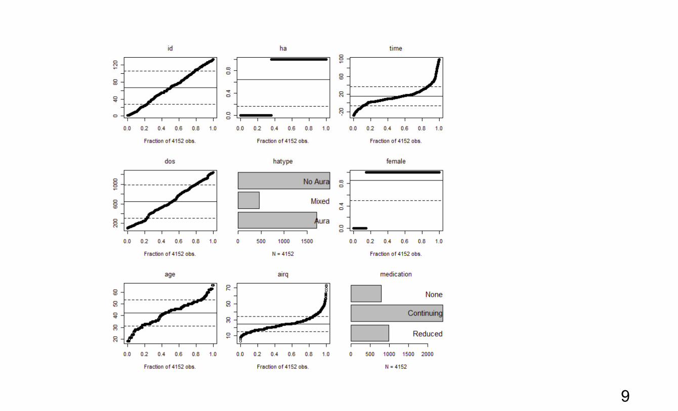
Consider 4,152 daily records of headache logs kept by 133 patients in a treatment program in which bio-feedback was used to attempt to reduce migraine frequency and severity. Patients entered the program at different times over a period of about 3 years. Patients were encouraged to begin their logs four weeks before the onset of treatment and to continue for one month afterwards, but only 55 patients have data preceding the onset of treatment.

Usage: > library( spidadev ) # loads MASS and nlme for glmmPQL

> data( migraines ) > ?migraines > ds <- migraines > xqplot(ds)

8

9

> ds$treat <- (ds$time > 0)*1

Create a dummy variable for treatment

> fit <- glmmPQL ( ha ~ treat, data = ds, + random = ~ 1 | id, + family = binomial) iteration 1 . . . iteration 5 > summary(fit) Linear mixed-effects model fit by maximum likelihood Data: ds AIC BIC logLik NA NA NA

Random effects: Formula: ~1 | id

NAs warn you that the fit is not really maximum likelihood

(Intercept) Residual StdDev: 1.479865 0.9410313

Variance function: Structure: fixed weights Formula: ~invwt

10

Fixed effects: ha ~ treat

Value Std.Error DF t-value p-value(Intercept) 0.8477543 0.1621571 4018 5.227980 0.0000treat -0.0164957 0.1038301 4018 -0.158872 0.8738

. . .

Number of Observations: 4152 Number of Groups: 133

The model used is a GLM with family = binomial, i.e. a logistic regression.

logit(Pr(ha)) 0.840.016treat

So the treatment reduces odds of headache to exp(0.016) 0.984 98% ,

i.e. a reduction of 2%

11

Overall view of the effect of treatment xyplot( ha ~ time, ds, panel = function(x, y, ...) {

panel.xyplot( x, jitter(y),...) panel.loess( x, y, ..., family = 'gaussian')})

Seems to make people worse before they get better (slightly) Maybe it’s short-term pain for long-term gain.

12

> ds$tdays <- ds$time / 10 > > # create a spline function:

> sp <- function(x) gsp( x, + knots = c(0,5,10,30,50)/10, + degree = c(1,2,2, 2, 2 ,1), + smooth = c(-1,1,1, 1, 1))

> fit <- glmmPQL ( ha ~ sp(tdays), data = ds, + random = ~ 1 | id, + family = binomial) iteration 1 iteration 2 iteration 3 iteration 4 iteration 5 > summary(fit) Linear mixed-effects model fit by maximum likelihood Data: ds AIC BIC logLik NA NA NA

Random effects: Formula: ~1 | id

(Intercept) Residual StdDev: 1.568552 0.9406108

13

Variance function: Structure: fixed weights Formula: ~invwt

Fixed effects: ha ~ sp(tdays) Value Std.Error DF t-value p-value

(Intercept) 0.720987 0.211794 4012 3.404190 0.0007 sp(tdays)D1(0) -0.122074 0.110583 4012 -1.103906 0.2697 sp(tdays)C(0).0 1.448669 0.429678 4012 3.371521 0.0008 sp(tdays)C(0).1 -3.241710 2.275235 4012 -1.424780 0.1543 sp(tdays)C(0).2 5.976928 5.544150 4012 1.078060 0.2811 sp(tdays)C(0.5).2 -6.482328 6.792881 4012 -0.954283 0.3400 sp(tdays)C(1).2 0.863025 1.594558 4012 0.541231 0.5884 sp(tdays)C(3).2 -0.498702 0.213875 4012 -2.331749 0.0198

Number of Observations: 4152Number of Groups: 133

> pred <- expand.grid( time = seq(-30,50,.5))

>

pred$tdays <- pred$time / 10

>

pred$ha.logit <- predict( fit, pred, level = 0) > xyplot( ha.logit ~ time, pred, type = 'l')

14

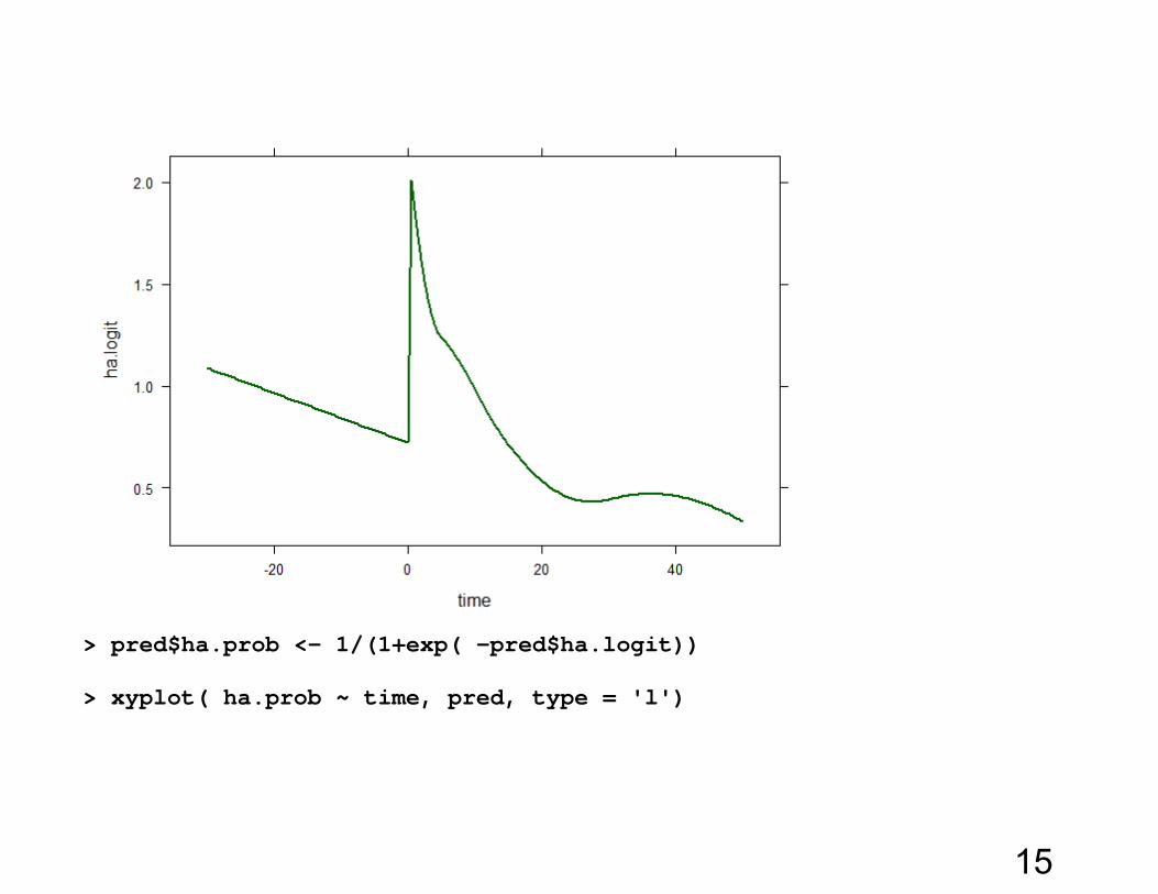
> pred$ha.prob <- 1/(1+exp( -pred$ha.logit))

> xyplot( ha.prob ~ time, pred, type = 'l')

15

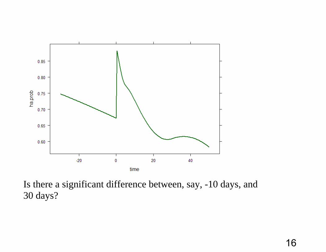
Is there a significant difference between, say, -10 days, and 30 days?

16

sc(sp, x, D = 0, type = 1)

generates a portion of an L matrix. sp – spline x - where spline should be evaluated D - what to evaluate:

0: value 1: slope 2: curvature, etc.

type – at a knot: type = 0: on the left, type = 1: on the right, type = 2: ‘saltus’: right – left

17

> Lp <- sc(sp,x = c(-10,30)/10, D = 0)> Lp

oefficients Estimate Std.Error DF t-value p-value(Intercept) 0.720987 0.211590 4012 3.407474 0.00066sp(tdays)D1(0) -0.122074 0.110477 4012 -1.104971 0.26924sp(tdays)C(0).0 1.448669 0.429264 4012 3.374774 0.00075sp(tdays)C(0).1 -3.241710 2.273042 4012 -1.426155 0.15390sp(tdays)C(0).2 5.976928 5.538806 4012 1.079100 0.28061sp(tdays)C(0.5).2 -6.482328 6.786334 4012 -0.955203 0.33953sp(tdays)C(1).2 0.863025 1.593021 4012 0.541754 0.58802sp(tdays)C(3).2 -0.498702 0.213669 4012 -2.333998 0.01964

D1(0) C(0).0 C(0).1 C(0).2 C(0.5).2 C(1).2 C(3).2g(-1) -1 0 0 0.0 0.000 0 0g(3+) 3 1 3 4.5 3.125 2 0

> wald(fit) numDF denDF F.value p.value

8 4012 15.43282 <.00001 C

> Lm <- cbind(0,Lp) > Ldiff <- rbind( Lm, diff= Lm[2,] - Lm[1,])

18

> Ldiff D1(0) C(0).0 C(0).1 C(0).2 C(0.5).2 C(1).2 C(3).2 g(-1) 0 -1 0 0 0.0 0.000 0 0 g(3+) 0 3 1 3 4.5 3.125 2 0 diff 0 4 1 3 4.5 3.125 2 0 > wald(fit, Ldiff) numDF denDF F.value p.value1 2 4012 5.930952 0.00268

Estimate Std.Error DF t-value p-valueg(-1) 0.122074 0.110477 4012 1.104971 0.26924g(3+) -0.277731 0.183149 4012 -1.516422 0.12949diff -0.399805 0.130583 4012 -3.061687 0.00222

19

MCMCglmmWhat’s a Markov Chain? A sequence of random variables (or vectors) where the distribution for the next one in the sequence (‘chain’) depends on the past only through the most recent value of the variable, i.e. the future depends on the past values of the variable (vector) only through the present values of the variable (vector). This is more general than it seems. If the next value depends on today’s and yesterday’s, we simply redefine the MC so it’s a vector of values for two successive days. What’s a Monte Carlo Markov Chain? A Markov Chain generated by a computer. What’s Markov Chain Monte Carlo? The process (and its study) of producing a Monte Carlo Markov Chain. Just say MCMC and you won’t have to think about this. 20

What’s so hot about Markov Chain Monte Carlo? It accomplishes the seemingly impossible … but only by going to an awful lot of trouble. From Andrieu (2003):

21

Example: Let’s say you really want to sample a bivariate distribution for (Y1,Y2). Note that Y here

is generic and the principle works with anything random (vector or variable): Ymis, , ,u .

But you can’t: you don’t have a way of generating random (Y1,Y2). But you do know something:

o You know to generate Y1 given Y2 and you know how to generate Y2 given Y1. You can do conditionals but you can’t do the joint or the marginal. You could generate random values, but you can’t get started. Note 1: This is not far fetched: This is exactly the problem with Ymis and in the

missing data problem. And in many other problems. Note 2: If you knew how to generate either marginally, say Y1, then you could

easily generate Y2 given Y1 and that would give you a sample for (Y1,Y2).

22

Solution: o Since you can’t generate a random Y1 to get started, just make it up! o Then keep going back and forth: Y2 from Y1, and then Y1 from Y2 and keep going for

a very long time. Under the right conditions, eventually, the starting value that you made up won’t matter and the (Y1,Y2) you get will be a random observation from the joint distribution. [burnin time]

o If you want more than one random observation, you can keep going but observations are dependent on each other so if you want them nearly independent, you will need to wait a while between the random observations you choose. [thinning the chain]

o The right conditions? No isolated islands of high probability surrounded by seas of low or no

probability. Otherwise you’ll be stuck on an island for a long time until your MCMC discovers the canoe. You might never discover that the world is really a larger place. Also, no single probability peak where you might get stuck.

23

Howtotellifit’sworking:o How do you know how long to burnin and to thin? o How do you know whether the results make sense?

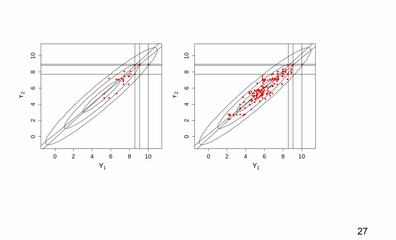
Example: Suppose you want to generate a random sample from the bivariate Normal with mean

(5,5), standard deviation 2 and correlation 0.95 But you haven’t yet discovered how to do this. However, you know how to generate a Y2

given Y1 and Y1 given Y2. Recall the missing data problem as an example: o If I knew Ymis I could estimate and if I knew I could impute Ymis. Given Y1 , I

could estimate beta. If only I could get started there’d be no problem because P(A) x P(B|A) = P( A and B). The MCMC solution: Start with a guess.

24

The MCMC hope: Eventually the initial choice won’t matter [burnin time] If you pick random observations far enough from each other, they will be close to

independent: [thinning] A fundamental principle: Under some conditions, if you know all the conditional distributions of each variable

given the others and there is a joint distribution that is consistent with these conditionals, then that joint distribution is unique, i.e. if there is one, there is only one.

The craft of MCMC: a) Is it working? b) What’s the right burnin? How long do I have to wait? c) What’s the right thinning? How many do I skip?

Will depend: mainly on the dependence of Y1 on Y2. If independent, the conditional = marginal and we really knew the marginal all along. We can take burnin = 1, thinning = 1/1.

25

0 2 4 6 8 10

02

46

810

Y1

Y2

0 2 4 6 8 10

02

46

810

Y1Y

2

26

0 2 4 6 8 10

02

46

810

Y1

Y2

0 2 4 6 8 10

02

46

810

Y1Y

2

27

The mean of Y1 in the sample is 5.902 The SE of the mean is:

1 2 0.22083n

So the mean of the sample is

5.902 5 4.10.220

SEs away from the population mean, which is much too large for such a sample. But the points in the sample are not independent. Using autocorrelation the effective sample size is:

> effectiveSize( Ysample) var1 var2 8.109846 9.606072

so the mean is only 1.28 SEs away.

0 2 4 6 8 10

02

46

810

Y1

Y2

28

MCMCdiagnostics> Ysample <- mcmc(Ysample) > plot(Ysample)

> Zsample <- mcmc( matrix( rnorm(2*83), ncol = 2)) > effectiveSize(Zsample) var1 var2 83 83 > plot(Zsample)

0 20 40 60 80

24

68

Iterations

Trace of var1

0 2 4 6 8 100.

000.

15

N = 83 Bandwidth = 0.6448

Density of var1

0 20 40 60 80

24

68

Iterations

Trace of var2

0 2 4 6 8 10

0.00

0.15

N = 83 Bandwidth = 0.6562

Density of var2 0 20 40 60 80

-20

2

Iterations

Trace of var1

-4 -2 0 2 4

0.0

0.2

0.4

N = 83 Bandwidth = 0.3756

Density of var1

0 20 40 60 80-2

02

Iterations

Trace of var2

-2 0 2 4

0.00

0.20

N = 83 Bandwidth = 0.4714

Density of var2

29

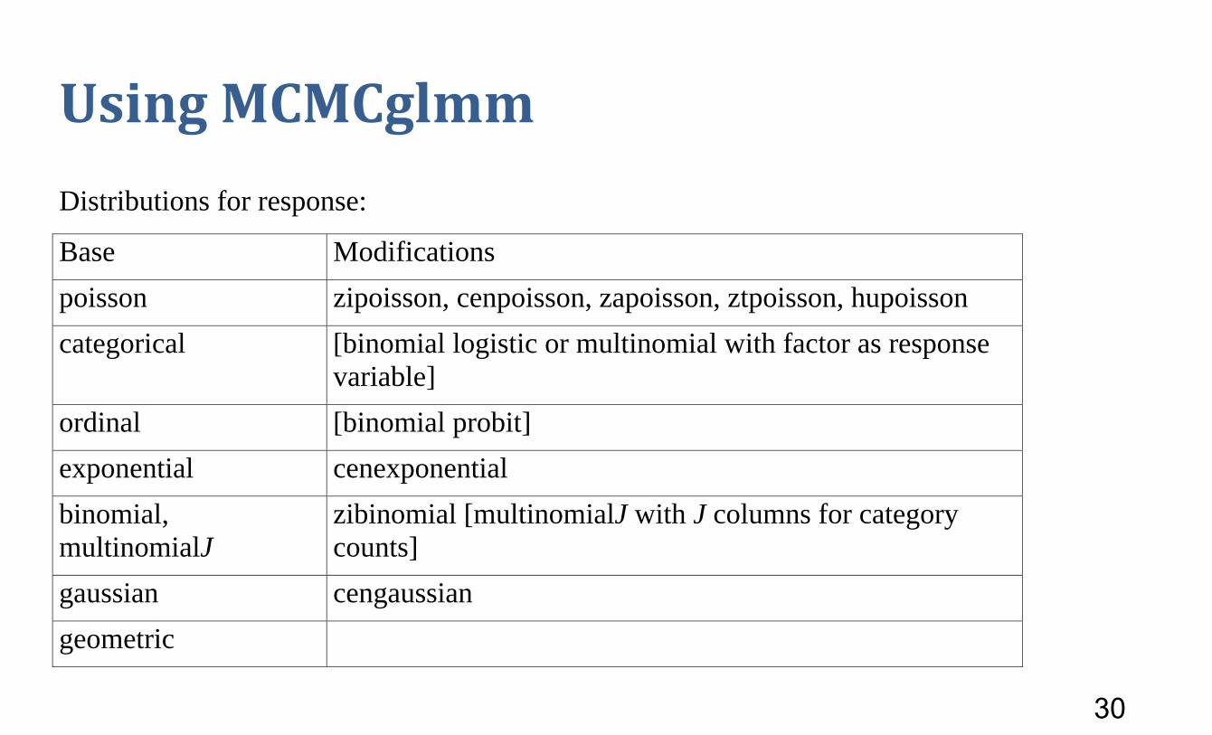
UsingMCMCglmm Distributions for response:

Base Modifications poisson zipoisson, cenpoisson, zapoisson, ztpoisson, hupoisson categorical [binomial logistic or multinomial with factor as response

variable] ordinal [binomial probit] exponential cenexponential binomial, multinomialJ

zibinomial [multinomialJ with J columns for category counts]

gaussian cengaussian geometric

30

Modifications: cen censoring: some values can be at floor or

ceiling, can vary from case to case zi zero-inflated, e.g. 0’s over and above what

you would expect from a Poisson as shown by the frequencies of values >0.

za zero-altered: Could be too many or too few zeros

zt zero-truncated: Only observe values >0 and shape of Poisson for Y > 0 gives appropriate probabilities

hu hurdle: binomial to determine 0 or >0, zt if greater

Note 1: No negative binomial: but to the extent that the negative binomial is used to have an extra parameter for overdispersion, MCMCglmm might be better when its model is faithful to dynamics of process.

31

Note 2: Can handle multivariate with different distributions!! E.g. one component gaussian, other binomial. ‘family’ distributions can be supplied as variable in data frame.

Note 3: What it won’t do: non-linear models, but maybe we can try to manage with splines

Multivariate Generalised Linear Mixed Models

Description

Markov chain Monte Carlo Sampler for Multivariate Generalised Linear Mixed Models with special emphasis on correlated random effects arising from pedigrees and phylogenies (Hadfield 2010). Please read the course notes: vignette("CourseNotes", "MCMCglmm") or the overviewvignette("Overview", "MCMCglmm")

Usage MCMCglmm(fixed, random=NULL, rcov=~units, family="gaussian", mev=NULL, data,start=NULL, prior=NULL, tune=NULL, pedigree=NULL, nodes="ALL", scale=TRUE, nitt=13000, thin=10, burnin=3000, pr=FALSE, pl=FALSE, verbose=TRUE, DIC=TRUE, singular.ok=FALSE, saveX=TRUE, saveZ=TRUE, saveXL=TRUE, slice=FALSE, ginverse=NULL)

32

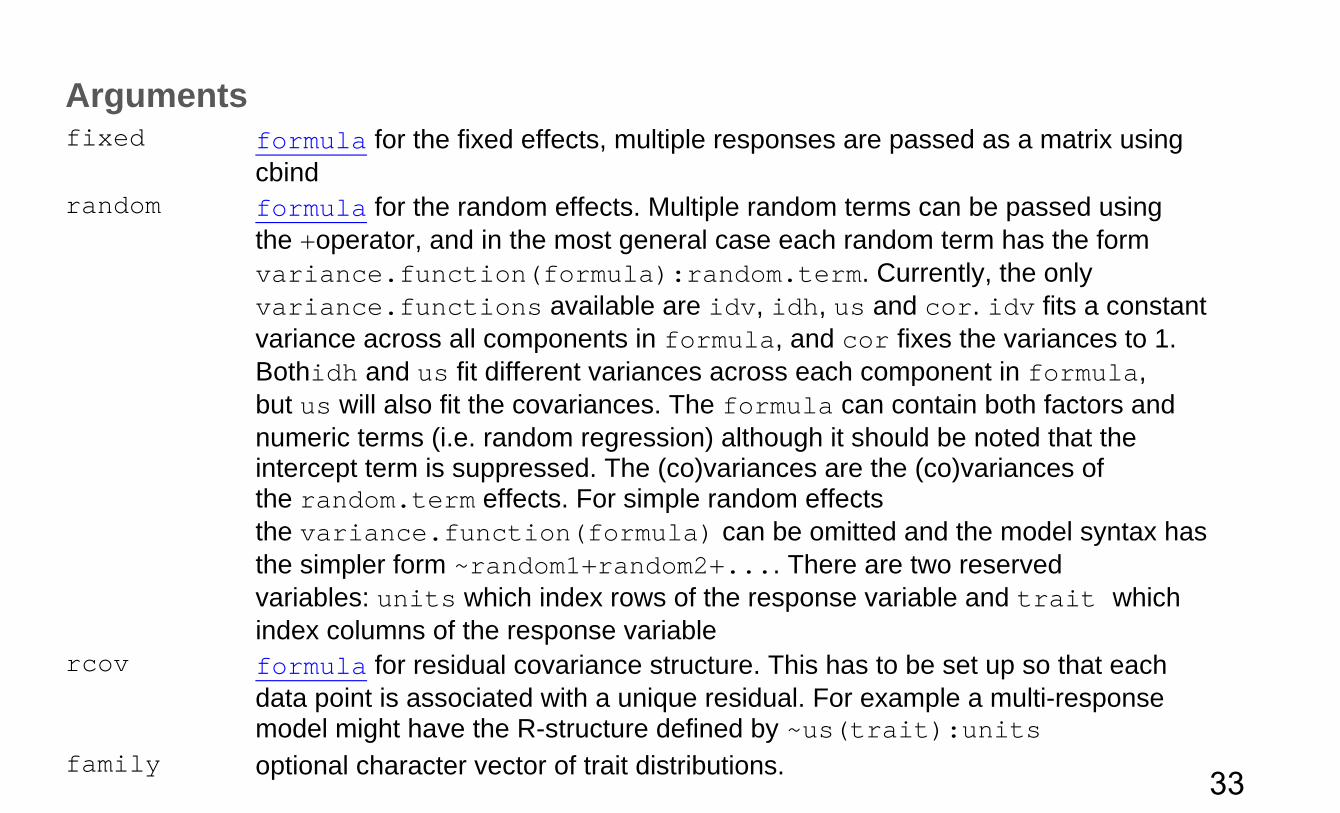
Arguments fixed formula for the fixed effects, multiple responses are passed as a matrix using

cbind random formula for the random effects. Multiple random terms can be passed using

the +operator, and in the most general case each random term has the form variance.function(formula):random.term. Currently, the only variance.functions available are idv, idh, us and cor. idv fits a constant variance across all components in formula, and cor fixes the variances to 1. Bothidh and us fit different variances across each component in formula, but us will also fit the covariances. The formula can contain both factors and numeric terms (i.e. random regression) although it should be noted that the intercept term is suppressed. The (co)variances are the (co)variances of the random.term effects. For simple random effects the variance.function(formula) can be omitted and the model syntax has the simpler form ~random1+random2+.... There are two reserved variables: units which index rows of the response variable and trait which index columns of the response variable

rcov formula for residual covariance structure. This has to be set up so that each data point is associated with a unique residual. For example a multi-response model might have the R-structure defined by ~us(trait):units

family optional character vector of trait distributions. 33

Currently, "gaussian", "poisson","categorical", "multinomial", "ordinal", "exponential","geometric", "cengaussian", "cenpoisson", "cenexponential","zipoisson", "zapoisson", "ztpoisson", "hupoisson" and"zibinomial" are supported, where the prefix "cen" means censored, the prefix"zi" means zero inflated, the prefix "za" means zero altered, the prefix "zt"means zero truncated and the prefix "hu" means hurdle. If NULL, data needs to contain a family column.

mev optional vector of measurement error variances for each data point for random effect meta-analysis.

data data.frame

start optional list having 4 possible elements: R (R-structure) G (G-structure) and liab (latent variables or liabilities) should contain the starting values where G itself is also a list with as many elements as random effect components. The fourth element QUASI should be logical: if TRUE starting latent variables are obtained heuristically, if FALSE then they are sampled from a Z-distribution

prior optional list of prior specifications having 3 possible elements: R (R-structure) G (G-structure) and B (fixed effects). B is a list containing the expected value (mu) and a (co)variance matrix (V) representing the strength of belief: the defaults are B$mu=0 and B$V=I*1e+10, where where I is an identity matrix of appropriate dimension. The priors for the variance structures (R and G) are lists with the expected (co)variances (V) and degree of belief parameter (nu) for the

34

inverse-Wishart, and also the mean vector (alpha.mu) and covariance matrix (alpha.V) for the redundant working parameters. The defaults are nu=0, V=1, alpha.mu=0, and alpha.V=0. When alpha.V is non-zero, parameter expanded algorithms are used.

tune optional (co)variance matrix defining the proposal distribution for the latent variables. If NULL an adaptive algorithm is used which ceases to adapt once the burn-in phase has finished.

nitt number of MCMC iterations thin thinning interval burnin burnin pr logical: should the posterior distribution of random effects be saved? pl logical: should the posterior distribution of latent variables be saved? verbose logical: if TRUE MH diagnostics are printed to screen DIC logical: if TRUE deviance and deviance information criterion are calculated singular.ok logical: if FALSE linear dependencies in the fixed effects are removed.

if TRUE they are left in and estimated, although all information comes from the prior

saveX logical: save fixed effect design matrix saveZ logical: save random effect design matrix saveXL logical: save structural parameter design matrix 35

slice logical: should slice sampling be used? Only applicable for binary trials with independent residuals

ginverse a list of sparse inverse matrices (solve(A)) that are proportional to the covariance structure of the random effects. The names of the matrices should correspond to columns in data that are associated with the random term. All levels of the random term should appear as rownames for the matrices.

Value Sol Posterior Distribution of MME solutions, including fixed effects VCV Posterior Distribution of (co)variance matrices CP Posterior Distribution of cut-points from an ordinal model Liab Posterior Distribution of latent variables Fixed list: fixed formula and number of fixed effects Random list: random formula, dimensions of each covariance matrix, number of levels per

covariance matrix, and term in random formula to which each covariance belongs Residual list: residual formula, dimensions of each covariance matrix, number of levels per

covariance matrix, and term in residual formula to which each covariance belongs Deviance deviance -2*log(p(y|...)) DIC deviance information criterion X sparse fixed effect design matrix

36

Z sparse random effect design matrix XL sparse structural parameter design matrix error.term residual term for each datum family distribution of each datum

37

Non‐mixedexample:OverdispersedPoissonwitha‘real’model

> library(MCMCglmm) > ?Traffic > head(Traffic) year day limit y 1 1961 1 no 9 2 1961 2 no 11 3 1961 3 no 9 4 1961 4 no 20 5 1961 5 no 31 6 1961 6 no 26 > xqplot(Traffic) > tab( Traffic, ~ year + limit) limit year no yes Total 1961 71 21 92 1962 44 48 92 Total 115 69 184 > histogram( ~ y| + paste(year)*paste('limit =',limit), + Traffic)

y

Per

cent

of T

otal

0

10

20

30

10 20 30 40 50

yearno

yearno

yearyes

10 20 30 40 50

0

10

20

30

yearyes

38

Dataset: Number of accidents per day in Sweden according to Year Limit: whether a speed limit was enforced on that day Day of the year (only about 80 days per year)

It is natural to model y = number of road accidents in a day as a Poisson random variable. The Poisson would be the correct distribution of the number of accidents if 1) On a given day, everyone has the same probability of an

accident 2) Accidents are independent. 3) There is no unexplained heterogeneity: All days that are

predicted to have the same number of expected accidents do, in fact, have the same number of expected accidents.

Any violation will tend to make you model fishy -- an ‘overdispersed’ Poisson. > Traffic$yr <- factor(Traffic$year) > fit <- glm( y ~ yr + limit + day, Traffic, + family = 'poisson') > summary(fit) Call:

39

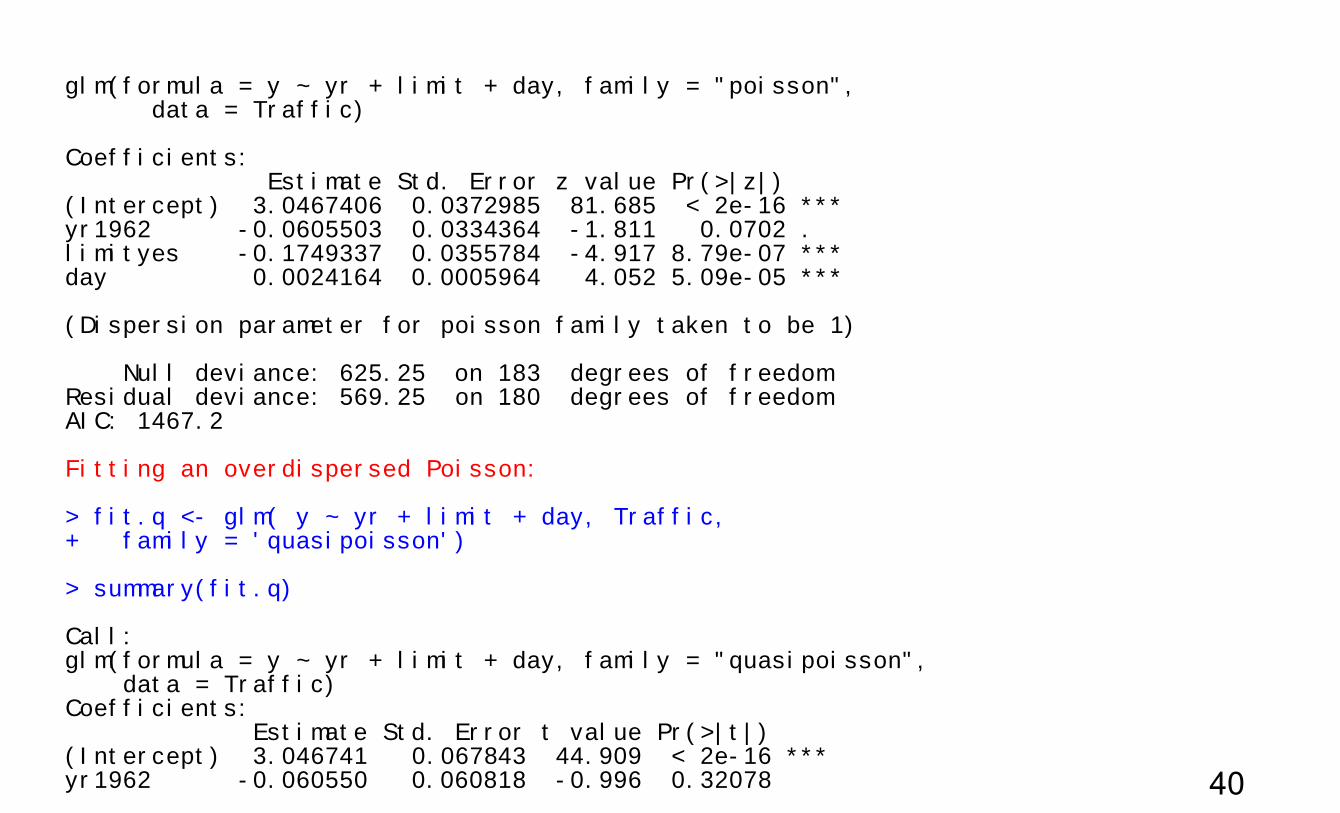
glm(formula = y ~ yr + limit + day, family = "poisson", data = Traffic) Coefficients: Estimate Std. Error z value Pr(>|z|) (Intercept) 3.0467406 0.0372985 81.685 < 2e-16 *** yr1962 -0.0605503 0.0334364 -1.811 0.0702 . limityes -0.1749337 0.0355784 -4.917 8.79e-07 *** day 0.0024164 0.0005964 4.052 5.09e-05 *** (Dispersion parameter for poisson family taken to be 1) Null deviance: 625.25 on 183 degrees of freedom Residual deviance: 569.25 on 180 degrees of freedom AIC: 1467.2 Fitting an overdispersed Poisson: > fit.q <- glm( y ~ yr + limit + day, Traffic, + family = 'quasipoisson') > summary(fit.q) Call: glm(formula = y ~ yr + limit + day, family = "quasipoisson", data = Traffic) Coefficients: Estimate Std. Error t value Pr(>|t|) (Intercept) 3.046741 0.067843 44.909 < 2e-16 *** yr1962 -0.060550 0.060818 -0.996 0.32078 40

limityes -0.174934 0.064714 -2.703 0.00753 ** day 0.002416 0.001085 2.227 0.02716 * (Dispersion parameter for quasipoisson family taken to be 3.308492) Null deviance: 625.25 on 183 degrees of freedom Residual deviance: 569.25 on 180 degrees of freedom AIC: NA

UsingMCMCglmm

~ ( exp(y Poisson X 2~ (0, )N I

Epsilon is NOT in the glm “poisson” model. Nor in the glm “quasipoisson” model. It allows for overdispersion due to unmodeled heterogeneity. It fits a Poisson model without assuming no overdispersion but fitting a real model, in contrast with the use of estimating equations with quasipoisson. 41

> fitmc <- MCMCglmm( y ~ yr + limit + day, + data = Traffic, + family = 'poisson') MCMC iteration = 0 Acceptance ratio for latent scores = 0.000239 MCMC iteration = 1000

.

. Acceptance ratio for latent scores = 0.389538 MCMC iteration = 13000 Acceptance ratio for latent scores = 0.388163

42

> summary(fitmc) # much more similar to quasipoisson than to poisson Iterations = 3001:12991 Thinning interval = 10 Sample size = 1000 DIC: 1197.334 R-structure: ~units post.mean l-95% CI u-95% CI eff.samp units 0.1008 0.0704 0.1359 816.6 Location effects: y ~ yr + limit + day post.mean l-95% CI u-95% CI eff.samp pMCMC (Intercept) 2.9923658 2.8533073 3.1146312 1000.0 <0.001 *** yr1962 -0.0677055 -0.1909837 0.0391579 1000.0 0.252 limityes -0.1720560 -0.2787613 -0.0400451 1000.0 0.004 ** day 0.0025657 0.0003546 0.0046178 880.5 0.030 *

43

> plot(fitmc, auto.layout = FALSE)

4000 8000 12000

2.8

3.0

3.2

Iterations

Trace of (Intercept)

2.8 3.0 3.2

02

46

N = 1000 Bandwidth = 0.01799

Density of (Intercept)

4000 8000 12000

-0.2

0.0

Iterations

Trace of yr1962

-0.3 -0.1 0.1

02

46

N = 1000 Bandwidth = 0.01563

Density of yr1962

4000 8000 12000

-0.3

-0.1

Iterations

Trace of limityes

-0.4 -0.2 0.0

02

46

N = 1000 Bandwidth = 0.01591

Density of limityes

4000 8000 12000

0.00

00.

006

Iterations

Trace of day

-0.002 0.002 0.006

015

035

0

N = 1000 Bandwidth = 0.0002808

Density of day

4000 8000 12000

0.06

0.14

Iterations

Trace of units

0.04 0.08 0.12 0.16

010

20

N = 1000 Bandwidth = 0.004323

Density of units

44

Eyeball training: > Z <- matrix(rnorm(2000),ncol=2) > head(Z) [,1] [,2] [1,] 0.2087386 -0.3803337 [2,] -2.6537110 -0.3144766 [3,] -1.0373284 -0.2916398 [4,] 0.2288955 -1.1388010 [5,] -1.3748541 -1.1512625 [6,] -0.7583837 -0.2082907 > plot( mcmc(Z))

0 200 600 1000

-30

2

Iterations

Trace of var1

-4 -2 0 2

0.0

0.2

N = 1000 Bandwidth = 0.2596

Density of var1

0 200 600 1000

-30

2

Iterations

Trace of var2

-2 0 2 4

0.00

0.20

N = 1000 Bandwidth = 0.2749

Density of var2

45

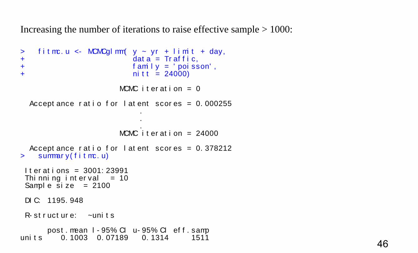
Increasing the number of iterations to raise effective sample > 1000: > fitmc.u <- MCMCglmm( y ~ yr + limit + day, + data = Traffic, + family = 'poisson', + nitt = 24000) MCMC iteration = 0 Acceptance ratio for latent scores = 0.000255

.

.

. MCMC iteration = 24000 Acceptance ratio for latent scores = 0.378212 > summary(fitmc.u) Iterations = 3001:23991 Thinning interval = 10 Sample size = 2100 DIC: 1195.948 R-structure: ~units post.mean l-95% CI u-95% CI eff.samp units 0.1003 0.07189 0.1314 1511

46

Location effects: y ~ yr + limit + day post.mean l-95% CI u-95% CI eff.samp pMCMC (Intercept) 2.9901543 2.8535135 3.1127372 1888 <5e-04 *** yr1962 -0.0655085 -0.1796330 0.0537198 1934 0.2724 limityes -0.1695618 -0.2992701 -0.0470397 1832 0.0114 * day 0.0026028 0.0003648 0.0046528 1882 0.0133 *

MCMCglmmwithamixedmodel > head(ds) id ha time dos hatype female age airq medication treat 1 1 1 -11 753 Aura 1 30 9 Continuing FALSE 2 1 1 -10 754 Aura 1 30 7 Continuing FALSE 3 1 1 -9 755 Aura 1 30 10 Continuing FALSE 4 1 1 -8 756 Aura 1 30 13 Continuing FALSE 5 1 1 -7 757 Aura 1 30 18 Continuing FALSE 6 1 1 -6 758 Aura 1 30 19 Continuing FALSE > ds $ treat <- 1*ds$treat > ds $ time.eff <- with(ds, exp(-time/13)*treat) > prior <- list( R = list(V=.05,nu=0,fix=1), + G = list(G1=list(V=diag(3), nu = .02))) > ds $ id <- factor( ds $ id ) > ds $ treat <- 1*ds$treat > ds $ time.eff <- with(ds, exp(-time/13)*treat) > 47

> prior <- list( R = list(V=.05,nu=0,fix=1), + G = list(G1=list(V=diag(3), nu = .02))) > > ds $ id <- factor( ds $ id ) > > fit4mc<- MCMCglmm ( ha ~ (treat + I( exp( - time / 13) * treat)) * medication , + data = ds, + family = "categorical", + random = ~ us( 1 + treat + time.eff):id, + prior = prior) MCMC iteration = 0 Acceptance ratio for latent scores = 0.000400 MCMC iteration = 1000 Acceptance ratio for latent scores = 0.428833 .

.

. MCMC iteration = 13000 Acceptance ratio for latent scores = 0.457138

48

> summary(fit4mc) Iterations = 3001:12991 Thinning interval = 10 Sample size = 1000 DIC: 4155.28 G-structure: ~us(1 + treat + time.eff):id post.mean l-95% CI u-95% CI eff.samp (Intercept):(Intercept).id 1.64437 0.79660 2.53289 31.365 treat:(Intercept).id 0.08521 -0.84724 0.83576 8.879 time.eff:(Intercept).id 0.18009 -0.57144 0.95664 14.401 (Intercept):treat.id 0.08521 -0.84724 0.83576 8.879 treat:treat.id 1.78350 0.56580 3.25219 11.060 time.eff:treat.id -1.56453 -2.74539 -0.06871 8.787 (Intercept):time.eff.id 0.18009 -0.57144 0.95664 14.401 treat:time.eff.id -1.56453 -2.74539 -0.06871 8.787 time.eff:time.eff.id 2.25575 0.03524 5.30354 3.345 R-structure: ~units post.mean l-95% CI u-95% CI eff.samp units 0.05 0.05 0.05 0

49

Location effects: ha ~ (treat + I(exp(-time/13) * treat)) * medication post.mean l-95% CI u-95% CI eff.samp pMCMC (Intercept) 1.61481 0.87917 2.44988 38.54 <0.001 *** treat -0.63092 -1.52981 0.08006 45.71 0.130 I(exp(-time/13) * treat) 2.80017 1.61635 3.73388 15.80 <0.001 *** medicationContinuing -0.80660 -1.74130 0.12437 34.43 0.094 . medicationNone -1.19420 -2.28772 -0.22304 79.32 0.016 * treat:medicationContinuing 0.35670 -0.60453 1.36830 39.08 0.476 treat:medicationNone -0.95212 -2.05963 0.14111 66.04 0.102 I(exp(-time/13) * treat):medicationContinuing -1.43442 -2.67162 0.12373 7.48 0.090 . I(exp(-time/13) * treat):medicationNone -1.14386 -2.59092 0.25944 25.79 0.120 > wald(fit4mc, 'medication') numDF denDF F.value p.value medication 6 Inf 5.48184 1e-05 Coefficients Estimate Std.Error DF t-value p-value medicationContinuing -0.806599 0.485507 Inf -1.661353 0.09664 medicationNone -1.194200 0.530661 Inf -2.250399 0.02442 treat:medicationContinuing 0.356696 0.505269 Inf 0.705952 0.48022 treat:medicationNone -0.952119 0.582397 Inf -1.634828 0.10209 I(exp(-time/13) * treat):medicationContinuing -1.434419 0.743038 Inf -1.930479 0.05355 I(exp(-time/13) * treat):medicationNone -1.143860 0.735718 Inf -1.554754 0.12000 Coefficients Lower 0.95 Upper 0.95 medicationContinuing -1.758176 0.144978 medicationNone -2.234277 -0.154123 treat:medicationContinuing -0.633613 1.347005 treat:medicationNone -2.093596 0.189358 I(exp(-time/13) * treat):medicationContinuing -2.890747 0.021908 I(exp(-time/13) * treat):medicationNone -2.585839 0.298120 50

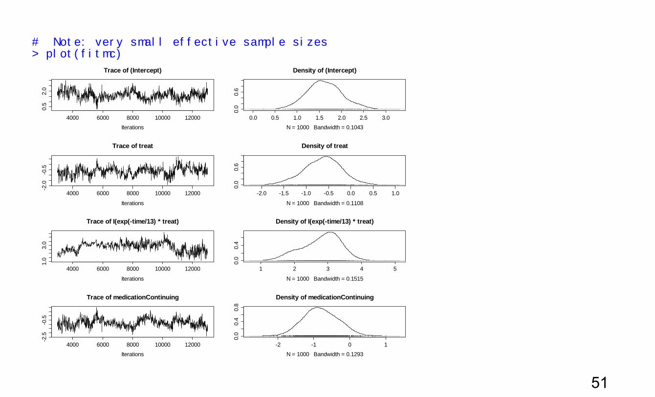
# Note: very small effective sample sizes > plot(fitmc)

4000 6000 8000 10000 12000

0.5

2.0

Iterations

Trace of (Intercept)

0.0 0.5 1.0 1.5 2.0 2.5 3.0

0.0

0.6

N = 1000 Bandwidth = 0.1043

Density of (Intercept)

4000 6000 8000 10000 12000

-2.0

-0.5

Iterations

Trace of treat

-2.0 -1.5 -1.0 -0.5 0.0 0.5 1.0

0.0

0.6

N = 1000 Bandwidth = 0.1108

Density of treat

4000 6000 8000 10000 12000

1.0

3.0

Iterations

Trace of I(exp(-time/13) * treat)

1 2 3 4 5

0.0

0.4

N = 1000 Bandwidth = 0.1515

Density of I(exp(-time/13) * treat)

4000 6000 8000 10000 12000

-2.5

-0.5

Iterations

Trace of medicationContinuing

-2 -1 0 1

0.0

0.4

0.8

N = 1000 Bandwidth = 0.1293

Density of medicationContinuing

51

4000 6000 8000 10000 12000

-3-1

Iterations

Trace of medicationNone

-3 -2 -1 0 1

0.0

0.4

N = 1000 Bandwidth = 0.1413

Density of medicationNone

4000 6000 8000 10000 12000

-1.0

0.5

Iterations

Trace of treat:medicationContinuing

-1 0 1 2

0.0

0.4

0.8

N = 1000 Bandwidth = 0.1329

Density of treat:medicationContinuing

4000 6000 8000 10000 12000

-3-1

Iterations

Trace of treat:medicationNone

-3 -2 -1 0 10.

00.

30.

6

N = 1000 Bandwidth = 0.1551

Density of treat:medicationNone

4000 6000 8000 10000 12000

-3-1

Iterations

Trace of I(exp(-time/13) * treat):medicationContinuing

-4 -3 -2 -1 0 1

0.0

0.3

N = 1000 Bandwidth = 0.1978

Density of I(exp(-time/13) * treat):medicationContinuing

52

4000 6000 8000 10000 12000

-3-1

1

Iterations

Trace of I(exp(-time/13) * treat):medicationNone

-4 -3 -2 -1 0 1 2

0.0

0.3

N = 1000 Bandwidth = 0.192

Density of I(exp(-time/13) * treat):medicationNone

4000 6000 8000 10000 12000

0.5

1.5

2.5

3.5

Iterations

Trace of (Intercept):(Intercept).id

0 1 2 3

0.0

0.4

0.8

N = 1000 Bandwidth = 0.1177

Density of (Intercept):(Intercept).id

4000 6000 8000 10000 12000

-1.5

-0.5

0.5

Iterations

Trace of treat:(Intercept).id

-1.5 -1.0 -0.5 0.0 0.5 1.0 1.5

0.0

0.4

0.8

N = 1000 Bandwidth = 0.1096

Density of treat:(Intercept).id

53

4000 6000 8000 10000 12000

-1.0

0.0

1.0

Iterations

Trace of (Intercept):time.eff.id

-1.0 -0.5 0.0 0.5 1.0 1.5

0.0

0.4

0.8

N = 1000 Bandwidth = 0.1061

Density of (Intercept):time.eff.id

4000 6000 8000 10000 12000

-4-3

-2-1

0

Iterations

Trace of treat:time.eff.id

-4 -3 -2 -1 0

0.0

0.2

0.4

0.6

N = 1000 Bandwidth = 0.1817

Density of treat:time.eff.id

4000 6000 8000 10000 12000

02

46

8

Iterations

Trace of time.eff:time.eff.id

0 2 4 6 8 10

0.00

0.10

0.20

0.30

N = 1000 Bandwidth = 0.4308

Density of time.eff:time.eff.id

54

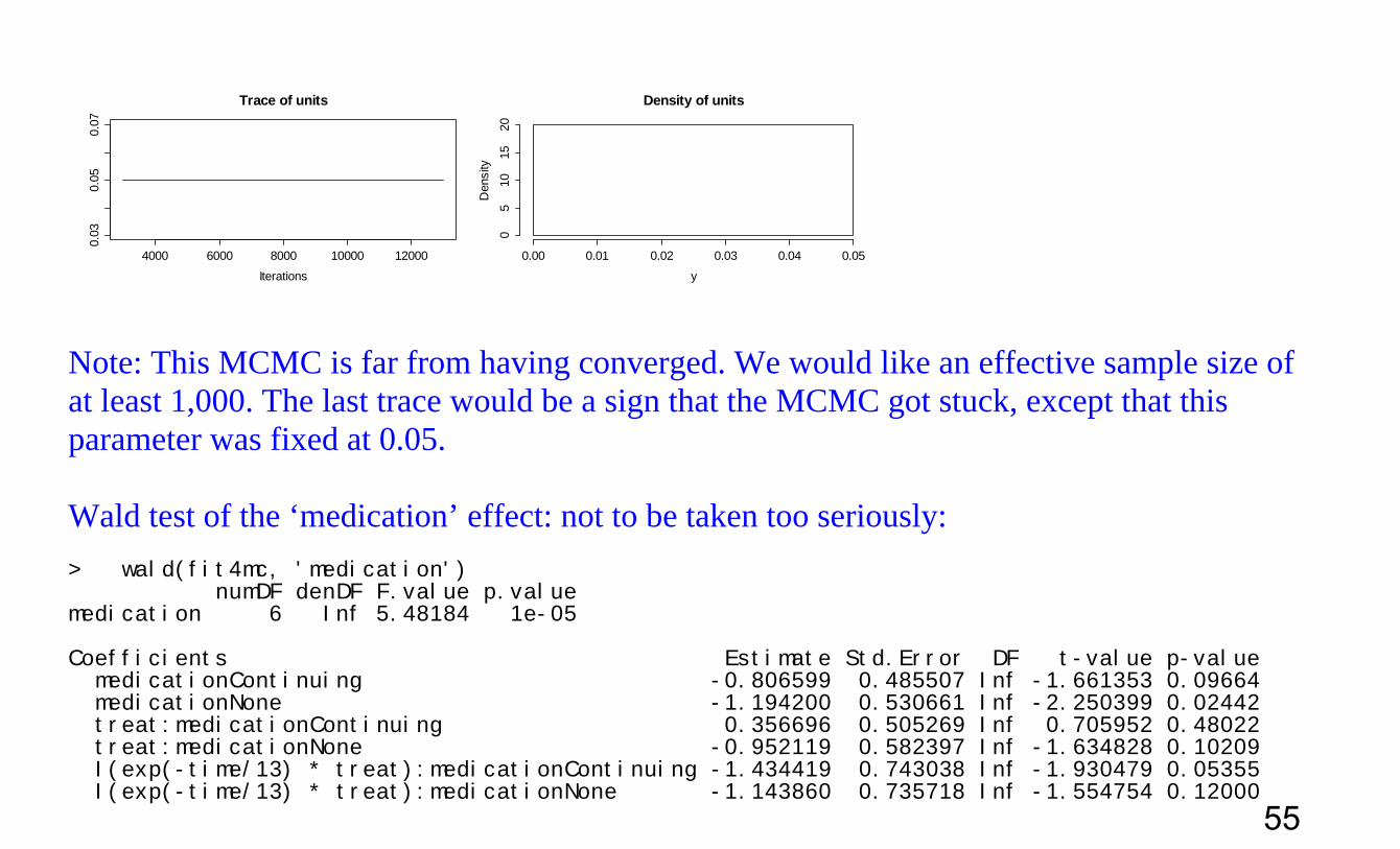
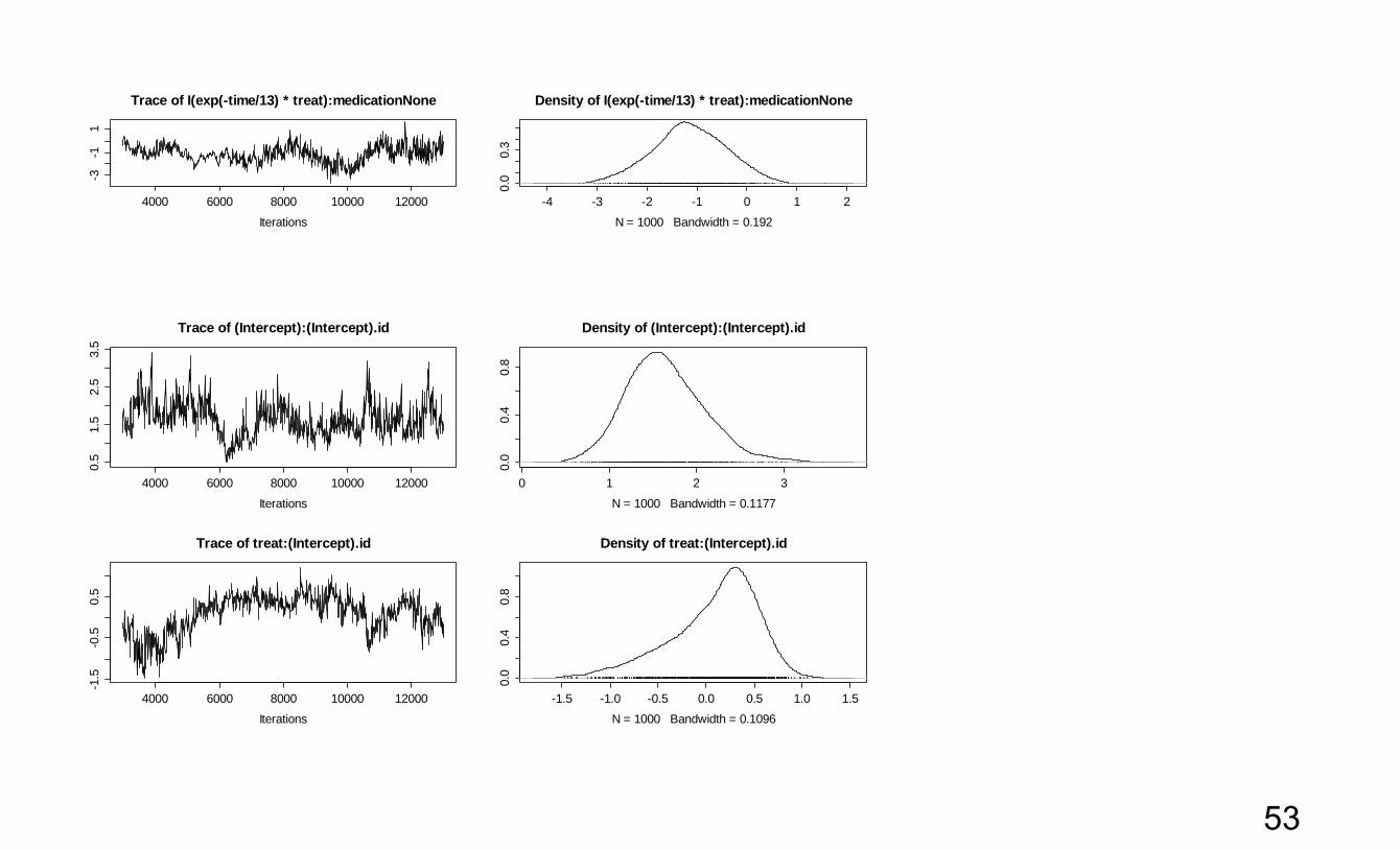
Note: This MCMC is far from having converged. We would like an effective sample size of at least 1,000. The last trace would be a sign that the MCMC got stuck, except that this parameter was fixed at 0.05. Wald test of the ‘medication’ effect: not to be taken too seriously: > wald(fit4mc, 'medication') numDF denDF F.value p.value medication 6 Inf 5.48184 1e-05 Coefficients Estimate Std.Error DF t-value p-value medicationContinuing -0.806599 0.485507 Inf -1.661353 0.09664 medicationNone -1.194200 0.530661 Inf -2.250399 0.02442 treat:medicationContinuing 0.356696 0.505269 Inf 0.705952 0.48022 treat:medicationNone -0.952119 0.582397 Inf -1.634828 0.10209 I(exp(-time/13) * treat):medicationContinuing -1.434419 0.743038 Inf -1.930479 0.05355 I(exp(-time/13) * treat):medicationNone -1.143860 0.735718 Inf -1.554754 0.12000

4000 6000 8000 10000 12000

0.03

0.05

0.07

Iterations

Trace of units

y

Den

sity

0.00 0.01 0.02 0.03 0.04 0.05

05

1015

20

Density of units

55

Why does R: 2 = 0.05 work?

With no 2 if p̂ for a points gets close to 1 or 0, the variance for that point

becomes close to 0 which makes the model stick to the point.

Keeping a minimal variance for each point prevents the model from sticking to them.

What to do next:

1) Consider centering random effects if their variance matrix approaches singularity. 2) Increase nitt, burnin and thin by a factor, perhaps 100, so

So nitt = 130000, burnin = 30000, thin = 1000 -- Might take all night

3) Explore the lab on GLMMs. 4) Read Jarrod Hadfields’s MCMCglmm Course Notes (2012)

56