spin squeezing and entanglement with room temperature ...€¦ · grandfather, doctor shen, gave me...
TRANSCRIPT

Spin squeezing and entanglement withroom temperature atoms for quantum
sensing and communication
Heng Shen
Niels Bohr Institute, University of Copenhagen
Academic supervisor:Prof. Eugene S. Polzik
This dissertation is submitted for the degree of
Doctor of Philosophy
December 2014


Summary
In this thesis, different experiments on spin squeezing and entanglement involving roomtemperature ensembles of Cesium atoms are described. The key method is the off-resonantFaraday interaction of spin-polarized atomic ensemble with a light field.
Quantum backaction evading measurement of one quadrature of collective spin compo-nents by stroboscopically modulating the intensity of probe beam at twice Larmor frequencyis used to generate the spin-squeezed state. A spin-squeezed state conditioned on the light-polarization measurement with 2.2±0.3dB noise reduction below the spin projection noiselimit for the measured quadrature has been observed.
In the radio-frequency atomic magnetometry, a transverse rf magnetic field resonant withthe atomic Larmor frequency causes the polarized spin ensemble to precess and the angleof precession is proportional to the rf magnetic field, which is measured with a weak off-resonant linearly polarized probe beam. A projection noise limited optical magnetometerat room temperature with an rf magnetic-field sensitivity of 158±1fT/
√Hz and 2D spatial
resolution of 300µm is reported. Furthermore, using spin-squeezing of atomic ensemble,the sensitivity of magnetometer is improved.
Deterministic continuous variable teleportation between two distant atomic ensemblesis demonstrated, where the light-atom entanglement establishes the non-local channel toteleport the spin information from one ensemble to the other. The fidelity of teleportatingdynamically changing sequence of spin states surpasses a classical benchmark, demonstrat-ing the true quantum teleportation.
Resumé
Denne afhandling beskriver adskillige eksperimenter med spin-sammenpresning ("squeez-ing") og sammenfiltring, som benytter ensembler af cæsiumatomer ved stuetemperatur.Afgørende til forsøgene er den Faraday vekselvirkning mellem spin-polariseret atomer oglys. Hovedrollen bliver spillet af mikrofremstillet glasbeholdere af atomer på gasform,koblet til en optisk kavitet.

iv
For at skabe et spin-sammenpresset tilstand måles der en kvadratur af den kollektivespin-komponent Jz på sådan et måde, at den såkaldte kvante "back-action" omgås. Teknikkener at modulere probe-lysets intensitet stroboskopisk, på en frekvens to gang så større somLarmor-frekvensen. Støjen af det spin-sammenpresset tilstand ligger 2.2 ± 0.3dB undergrænsen for spin-projektionsstøjen.
I radiofrekvens atom-optisk magnetometri, et tværsgående rf magnetisk felt påresonansmed atomernes Larmor-frekvens gøre den polariseret spin-ensembel til at præcessere. Præ-cessionsvinklen er proportional med magnetfeltet, der bliver målt med brug af svag lineært-polariseret probe-lys. Der presenteres en projektionsstøjsbegrænset optisk magnetometerved stuetemperatur med sensitivitet 158± 1fT/
√Hz og rumlig resolution 300µm. Sensi-
tiviteten forbedres endnu mere med hjælp af spin-sammenpresningen.Der vises også deterministisk kontinuerlig-variabel teleportation mellem to atomare en-
sembler på stor afstand. I denne sammenhæng sammenfiltring mellem lys og atomer etablereren ikke-lokal kanal til at teleportere spin-information fra den ene ensembel til den anden.Fideliteten af at teleportere spin-tilstande, som ændrer sig på en dynamisk måde, overgårdet klassiske benchmark. Derfor er der tale om den ægte kvante-teleportation.

Abstract
In this thesis, different experiments on spin squeezing and entanglement involving roomtemperature ensembles of Cesium atoms are described. The key method is the off-resonantFaraday interaction of spin-polarized atomic ensemble with a light field. And the key com-ponent is the micro-fabricated vapor cell coupled into an optical cavity. Quantum backactionevading measurement of one quadrature of collective spin components by stroboscopicallymodulating the intensity of probe beam at twice Larmor frequency is used to generate thespin-squeezed state. A projection noise limited optical magnetometer at room tempera-ture is reported. Furthermore, using spin-squeezing of atomic ensemble, the sensitivity ofmagnetometer is improved. Deterministic continuous variable teleportation between twodistant atomic ensembles is demonstrated. The fidelity of teleportating dynamically chang-ing sequence of spin states surpasses a classical benchmark, demonstrating the true quantumteleportation.


Preface
The work presented in this dissertation is a summary of research carried out between Sep2011 and Jan 2015 as a PhD candidate in the Danish National Research Foundation Centerfor Quantum Optics (QUANTOP group) led by professor Eugene Polzik at the Niels BohrInstitute, University of Copenhagen. In the beginning of my PhD study, I had the pleasureof working on the project of quantum teleportation between two atomic ensembles in themarcocells with Hanna Krauter, Daniel Salart and Jonas Meyer Petersen when I learnt thedaily routines in the lab from them. In the following three years, the focus has shiftedfrom the experimental research on the macrocell to the fundamental investigation towardsapplication on the micro-fabricated vapor cells, and Eugene gave me this good opportunityto be the first PhD student working on this project, which is the main part of this thesis.
I am grateful to Prof. Eugene Polzik for giving me the opportunity to work in QUAN-TOP on this completely new project. Although time flies fast, I still remember the first timeI had a skype conversation with him through the unstable Internet, and several times fruitfuldiscussion with him during my first visit in Denmark. He really taught me a lot not only inphysics but also in the attitude to the life, which helped me smoothly transit from an opticalexperimentalist to a beginner on the atomic physics, and from the Chinese eduction modeto the European one. Without Eugene’s enthusiasm and physical intuition, I would have nochance to present the results here.
I thank Giorgos Vasilakis very much for closely working with me more than two years.We had countless interesting conversations, both about physics and philosophical topics. Heis not only a very good colleague in the lab but also a nice friend in the daily life. I enjoyedthe good time with his big family, especially with Penelope.
I would like to thank Hanna Krauter and Jonas Meyer Petersen who gave me lots ofhelp to start my study in the lab and the life abroad. Although the overlapping with Hannawas very short, she was trying her best to give me supports. I thank Daniel Salart for hissupport on the experiment, and we have had a very good collaboration for three years. I alsowant to thank Misha Balabas for the good times when developing the microcells together.The visiting PhD student Bing Chen is a good collaborator who made an enthusiastic con-

viii
tribution to the experiment, and is also one of my close friends keeping talking with me inChinese. During my time at QUANTOP I have also had the opportunity to work with other"Cellmates" including Kasper Jensen, Anne Fabricant, Michael Zugenmaier, and RodrigoThomas. I would also like to acknowledge the members of QUANTOP group for a friendlyatmosphere during the years.
I also thank my big Chinese group including Pengfei, Haoran, Junjie, Yang, Guannan,Hairun, Haiyan, Tian, Qian, Ming and others for your warm company and support.
Last but not least I would like to thank my current and future family members. My deadgrandfather, Doctor Shen, gave me a nice education on the art and sociology which deeplyimpressed me. My parents, Doctor Shen and Doctor Guo, took care of me so long time andgave me the opportunity to reach different taste of food and cultures.

List of Publications
1. H. Krauter, D. Salart, C. A. Muschik, J. M. Petersen, Heng Shen, T. Fernholz, and E.S. Polzik, Deterministic quantum teleportation between distant atomic objects, NaturePhysics 9, 400 (2013).
2. G. Vasilakis, H. Shen1, K. Jensen, M. Balabas, D. Salart, B. Chen, E. S. Polzik,Generation of a squeezed state of an oscillator by stroboscopic back-action-evadingmeasurement, arXiv:1411.6289, 2014(submitted to Nature Physics).
3. H. Shen, G. Vasilakis, K. Jensen, M. Balabas, D. Salart, A. Fabricant, B. Chen, E. S.Polzik, Quantum noise limited cavity-enhanced radio-frequency atomic magnetome-ter, to be submitted.
1G. Vasilakis, H. Shen contribute equally to this work.


Table of contents
List of Publications ix
Table of contents xi
Nomenclature xiii
1 Introduation 11.1 Quantum information processing . . . . . . . . . . . . . . . . . . . . . . . 1
1.2 Quantum Metrology . . . . . . . . . . . . . . . . . . . . . . . . . . . . . . 2
1.3 Integrated quantum devices . . . . . . . . . . . . . . . . . . . . . . . . . . 2
1.4 Outline . . . . . . . . . . . . . . . . . . . . . . . . . . . . . . . . . . . . 3
2 Quantum interface between light and atoms 52.1 Canonical variables . . . . . . . . . . . . . . . . . . . . . . . . . . . . . . 5
2.1.1 Light . . . . . . . . . . . . . . . . . . . . . . . . . . . . . . . . . 5
2.1.2 Atoms . . . . . . . . . . . . . . . . . . . . . . . . . . . . . . . . . 7
2.2 Interaction between light and atoms . . . . . . . . . . . . . . . . . . . . . 9
2.2.1 Hamiltonian . . . . . . . . . . . . . . . . . . . . . . . . . . . . . 9
2.2.2 Propagation equations . . . . . . . . . . . . . . . . . . . . . . . . 11
2.2.3 Input output relations in Quantum Non-demolition interaction picture 13
2.2.4 Tensor interaction . . . . . . . . . . . . . . . . . . . . . . . . . . . 16
2.3 Entanglement between light and atoms . . . . . . . . . . . . . . . . . . . . 21
2.3.1 Introduction to quantum entanglement . . . . . . . . . . . . . . . . 21
2.3.2 Generation of the entanglement between light and atoms . . . . . . 23
2.4 Collective spin states in room temperature coated cells . . . . . . . . . . . 25
2.4.1 Coating . . . . . . . . . . . . . . . . . . . . . . . . . . . . . . . . 25
2.4.2 Thermal averaging . . . . . . . . . . . . . . . . . . . . . . . . . . 27

xii Table of contents
3 Experimental system 293.1 Laser system . . . . . . . . . . . . . . . . . . . . . . . . . . . . . . . . . 30
3.1.1 Probe light . . . . . . . . . . . . . . . . . . . . . . . . . . . . . . 303.1.2 Optical pumping . . . . . . . . . . . . . . . . . . . . . . . . . . . 32
3.2 Microcell . . . . . . . . . . . . . . . . . . . . . . . . . . . . . . . . . . . 333.2.1 Fabrication . . . . . . . . . . . . . . . . . . . . . . . . . . . . . . 333.2.2 Faraday angle . . . . . . . . . . . . . . . . . . . . . . . . . . . . . 363.2.3 T1 and T2 . . . . . . . . . . . . . . . . . . . . . . . . . . . . . . . 38
3.3 Optical cavity . . . . . . . . . . . . . . . . . . . . . . . . . . . . . . . . . 413.4 Preparation and characterization of the atomic state . . . . . . . . . . . . . 43
3.4.1 Magneto optical resonance . . . . . . . . . . . . . . . . . . . . . . 433.5 Coupling strength . . . . . . . . . . . . . . . . . . . . . . . . . . . . . . . 473.6 Quantum noise . . . . . . . . . . . . . . . . . . . . . . . . . . . . . . . . 49
3.6.1 Light noise . . . . . . . . . . . . . . . . . . . . . . . . . . . . . . 493.6.2 Reconstruction of the atomic spin noise . . . . . . . . . . . . . . . 52
4 Backaction evasion and conditional spin squeezing by stroboscopic probing 574.1 Stroboscopic probing . . . . . . . . . . . . . . . . . . . . . . . . . . . . . 57
4.1.1 Introduction . . . . . . . . . . . . . . . . . . . . . . . . . . . . . . 574.1.2 Protocol . . . . . . . . . . . . . . . . . . . . . . . . . . . . . . . . 58
4.2 Experimental demonstration of backaction evasion measurement . . . . . . 634.3 2dB-conditional spin squeezing . . . . . . . . . . . . . . . . . . . . . . . . 67
4.3.1 Introduction . . . . . . . . . . . . . . . . . . . . . . . . . . . . . . 684.3.2 Squeezing mechanism . . . . . . . . . . . . . . . . . . . . . . . . 684.3.3 Experimental realization . . . . . . . . . . . . . . . . . . . . . . . 704.3.4 Results . . . . . . . . . . . . . . . . . . . . . . . . . . . . . . . . 71
4.4 Conclusion and outlook . . . . . . . . . . . . . . . . . . . . . . . . . . . . 73
5 Cavity enhanced atomic magnetometer beyond the quantum noise limit 755.1 Introduction . . . . . . . . . . . . . . . . . . . . . . . . . . . . . . . . . . 755.2 Quantum noise limited RF magnetometer . . . . . . . . . . . . . . . . . . 76
5.2.1 A pulsed RF magnetometer . . . . . . . . . . . . . . . . . . . . . 765.2.2 Quantum noise limited RF magnetometer based on backaction eva-
sion measurement . . . . . . . . . . . . . . . . . . . . . . . . . . . 775.2.3 Experimental realization . . . . . . . . . . . . . . . . . . . . . . . 795.2.4 Results . . . . . . . . . . . . . . . . . . . . . . . . . . . . . . . . 81
5.3 Magnetic sensitivity beyond the quantum noise limit by spin squeezing . . 84
Table of contents xiii
5.3.1 Protocol . . . . . . . . . . . . . . . . . . . . . . . . . . . . . . . . 845.3.2 Experimental results . . . . . . . . . . . . . . . . . . . . . . . . . 85
5.4 Effect of optical cavity . . . . . . . . . . . . . . . . . . . . . . . . . . . . 865.5 Conclusion and outlook . . . . . . . . . . . . . . . . . . . . . . . . . . . . 88
6 Deterministic quantum teleportation between distant atomic objects 896.1 Introduction . . . . . . . . . . . . . . . . . . . . . . . . . . . . . . . . . . 896.2 Teleportation protocol . . . . . . . . . . . . . . . . . . . . . . . . . . . . . 90
6.2.1 Generation and distribution of the Einstein-Podolsky-Rosen entan-gled state . . . . . . . . . . . . . . . . . . . . . . . . . . . . . . . 91
6.2.2 Bell measurement at Alice’s station . . . . . . . . . . . . . . . . . 926.2.3 Classical communication and feedback at Bob’s station . . . . . . . 92
6.3 Experimental realization . . . . . . . . . . . . . . . . . . . . . . . . . . . 936.3.1 Experimental setup . . . . . . . . . . . . . . . . . . . . . . . . . . 936.3.2 Experimental results . . . . . . . . . . . . . . . . . . . . . . . . . 946.3.3 Fidelity . . . . . . . . . . . . . . . . . . . . . . . . . . . . . . . . 95
6.4 Conclusion and outlook . . . . . . . . . . . . . . . . . . . . . . . . . . . . 98
7 Conclusions and outlook 997.1 Conclusions . . . . . . . . . . . . . . . . . . . . . . . . . . . . . . . . . . 997.2 Outlook . . . . . . . . . . . . . . . . . . . . . . . . . . . . . . . . . . . . 100
Appendix A Details of the magnetic coil system 105
Appendix B Details of the microcell fabrication 111
Appendix C Phase-Locking and Frequency-Locking system 115
Bibliography 121


Chapter 1
Introduation
1.1 Quantum information processing
Since quantum teleportation was proposed by Bennett et. al. in 1993[1], theoretical andexperimental researches on quantum information have developed rapidly. As one applica-tion of quantum entanglement in the communication, quantum dense coding, which is away to transmit two bits of information through the manipulation of only one of two en-tangled quantum systems[2], has been experimentally demonstrated in both discrete andcontinuous quantum variable regimes[3, 4]. Furthermore, absolutely secure transmission ofsecret messages and the faithful transfer of unknown quantum states is promised by quantumcommunication. However, due to losses and decoherence in the channel, the communica-tion fidelity decreases exponentially with the channel length which makes the long-distancequantum communication difficult to be built realistically. In order to solve this problem, the-orists suggested to use atomic ensembles and linear optics components as quantum repeatersto improve the communication fidelity[5].
As another important application of quantum technology, quantum computer (QC) ad-mitting quantum superposition and entanglement attracts more and more attention and istreated as a milestone of modern science due to its promise of high-speed and powerfulcomputation capacities over the classical computer. So far, many exciting theoretical andexperimental tasks have been accomplished in both the discrete variable (DV) and contin-uous variable (CV)[6, 7, 8], such as Shor’s quantum factoring algorithm[9], which reducesrunning time from exponential to polynomial time with respect to the classical factorizationalgorithm. Besides quantum logic gates, quantum memory is also indispensable to a gen-uine quantum computer due to its synchronization function that ensures operations could betimed appropriately. In the CV regime, storing photonic information in the atomic ensem-bles, especially for the nonclassical CV of light, primarily relies on two different methods:

2 Introduation
one based on electromagnetically induced transparency (EIT)[10] and the other utilizing theoff-resonant Faraday interaction between light and atoms [11].
1.2 Quantum Metrology
Quantum metrology is the use of quantum techniques such as entanglement to make high-resolution and highly sensitive measurements of physical parameters, and to yield higherstatistical precision than purely classical approaches. Recently, squeezed vacuum statesof light has been used to improve the sensitivity of a gravitational-wave observatory inGEO200 project[12]. It has been suggested that spin-squeezed states of atomic ensem-bles can be prepared for the improvement of sensitivity in atomic spectroscopy, interfer-ometry and atomic clocks[13, 14, 15, 16]. Several schemes have been proposed to gener-ate the spin-squeezed states, including the direct interaction of spins[17], electron-nucleusentanglement[18], mapping of squeezed light onto atoms[19], multiple passes of light throughatoms[20] and a projective Faraday interaction based on quantum non-demolition measure-ment (QND)[21, 22]. Entangled states of atoms can also be used in metrology such as inatomic clocks where the projection noise of atoms limits the accuracy of the clock. Suchan entanglement-assisted atomic clock was demonstrated recently in our group[22]. In ad-dition, quantum teleportation allows for performing quantum sensing at a remote location,spatially separated from the location of the object.
1.3 Integrated quantum devices
Many quantum physical experiments have performed with bulk optics. However, complexquantum optical schemes, realized in bulk optics, suffer from severe drawbacks, as far asstability, and physical size are concerned. Therefore, people start to seek for a much morecompact and stable system which is promising in the real application, such as computerCPU and other integrated functional chips. For quantum photonics, the channel can be builtin the form of optical waveguide devices by using the ultrafast laser writing and other nanofabrication technologies. Shor’s algorithm has been realized on an integrated waveguidesilica-on-silicon chip[23]. On the other hand, the single photon source can also be integratedin the semiconductor chip, for example, solid-state QED where the quantum dot is stronglycoupled in the high Q optical cavity created by the photonic crystal with a defect[24]. Addi-tionally, in order to form the all-optical quantum communication and linear-optics quantumcomputing, not only single-photon sources and passive optical circuits, but also photon de-tectors are required. At present, researchers are trying to build photon detectors on the

1.4 Outline 3
chip using nano-fabrication technology based on III-V semiconductors[25]. Atomic en-sembles as a good candidate for many quantum protocols such as quantum repeater andquantum memory, are also suitable to be integrated on the chip as active elements basedon light-matter interaction. This type of quantum device can be made very compact inthe application. For example an integrated sensor package incorporating a VCSEL laser,an alkali-vapour cell, optics, and a detector has been constructed[26]. And Bose-EinsteinCondensation on an atom chip where cold atoms are magnetically trapped and guided us-ing the magnetic field produced by conductors on the surface is another topic with lots ofapplication such as atom interferometer and magnetometry on a chip[27].
1.4 Outline
This thesis is divided in three parts: the theoretical background containing Chapters 2, theexperimental methods with Chapters 3 and finally the description of the experiments ongeneration and application of spin squeezed state and entanglement in Chapters 4, 5 and 6.
To be specific, Chapter 2 gives a the details of a previously established theoretical ap-proach of light atom interface including the canonical description of atoms and light, interac-tion hamiltonian between light and atoms, especially the off-resonant Faraday interaction,input-output relations and the concept of thermal motion averaging and establishment ofentanglement between light and atoms, whose understanding is essential for the discussedexperiments.
In Chapter 3 the details of the experimental system are explained, including characteris-tic measures of atoms and light. Most importantly, the microcell as the key element of thisthesis is firstly shown in our work, including the fabrication and characterization. Opticalcavity and the quantum noise properties of the atomic and light system are then discussed.
Chapter 4 presents the experiment on the generation of spin-squeezed state by strobo-scopic backaction evading measurement based on the micro-fabricated vapor cell coupledinto an optical cavity. In Chapter 5 as an application of the established method of con-ditional spin squeezing, atomic magnetometer beyond the quantum noise limit is demon-strated. Chapter 6 details the experiment on teleportation between two atomic ensemblesand the theory behind the experiment.
The thesis is concluded in Chapter 7 where I summarize the main results in this thesisand give an outlook about the coming experiments based on the same setup.


Chapter 2
Quantum interface between light andatoms
In this section we describe the off-resonant dipole atom-light interaction utilizing the groundstate 6S1/2 to the excited state 6P3/2 transition in cesium where collective spin operators foratoms and Stokes operators for light are described in canonical operators in the languageof continuous variables. The interface between light and atoms provides the basis for theexperiments discussed in the thesis. Since most of the work presented in this thesis is inthe QND picture where the tensor interaction is negligible by using a larger blue detuningof the probe light, we focus on the equation of motion and the input-output relation thatare often used in the following chapter. However, we give some description of the tensorinteraction and entanglement that will be used to discuss the quantum teleportation betweentwo atomic ensembles. At the end of this chapter, the concept of motion averaging for thethermal atoms is discussed which is very important in the collective effect, and relates to thesingle photon generation in DLCZ scheme.
2.1 Canonical variables
2.1.1 Light
To describe the interaction between light and atom involved in all the experiments of thisthesis, the quantum state of light is characterized by the Stokes operators Sx,Sy and Sz, whichare given by the differences of the number operators npolarization of the photons polarized in

6 Quantum interface between light and atoms
different orthogonal bases. For the light propagating in z-direction we have
Sx =12(nx − ny)
Sy =12(n+45 − n−45)
Sz =12(nσ+ − nσ−),
(2.1)
where the indices x,y of npolarization represent the photons polarized in x- or y-direction and±45 label the photons polarized in ±45-direction, while σ± show the photons circularlypolarized in the left or right hand direction. The Stokes vector satisfies the commutation ofangular momentum
[Sy, Sz] = iSx, (2.2)
which shows the Heisenberg uncertainty principle as
Var(Sy) ·Var(Sz)≥⟨Sx⟩2
4. (2.3)
In the experiment, we always use x- or y- linearly polarized coherent light pulse to interactwith the atomic ensembles, which means Sx can be treated as a large classical value propor-tional to the flux of photons Φ = P/(hω) while P represents the optical power and hω is theenergy of single photon. The quantum variables Sy and Sz are the physical variables we areinterested in, and usually they have zero mean value since a collection of x-polarized pho-tons holds the equal probability for the polarization of ±45 or σ±. The canonical operatorsof light can be defined as
xL =Sy√|Sx|
, pL = σSXSz√|Sx|
,→ [xL, pL]≈ i, (2.4)
where σSx =±1depends on the sign of Sx. In the setting of the experiments involved in thisthesis a y-polarized coherent light pulse usually serves as the drive light as well as a phasereference for the x-polarized signal part which carries the interesting quantum fluctuation(that is the reason we use the polarization homodyne detection instead of typical homodynesystem with an addition strong local beam), and the canonical operators can be representedby the creation and annihilation operators ax and a†
x of light in x-polarization,
xL = 1√2(ax + a†
x), pL = 1√2i(ax − a†
x), (2.5)

2.1 Canonical variables 7
If Var(Sy) = Var(Sy) = ⟨Sx⟩/2 (i.e.Var(xL) = Var(pL) = 1/2) we say that the noise of Sy
or Sz is at the shot noise limit. Usually, one defines the creation and annihilation operatorsin time domain with the commutation relation [ax(t,z), a†
x(t′,z)] = δ (k−k′). In the position
space it will follow [ax(z, t), a†x(z
′, t)] = cδ (z− z′).
2.1.2 Atoms
We will describe the atomic states of an ensemble in terms of its collective spin in thedifferent directions, which is given by the sum of the total angular momenta of the individualatoms jk
i :
Ji =Na
∑k
jki (2.6)
with i= x,y,z. Since the ensemble contains such a vast amount of atoms those spin variablesare quasi continuous. The collective spin follows, as do the individual spins, the commuta-tion relation of angular momentum,
[Jy, Jz] = iJx, (2.7)
so the Heisenberg uncertainty principle reads
Var(Jy) ·Var(Jz)≥⟨Jx⟩2
4. (2.8)
In the experiments we discuss here, typically the atomic spins are all oriented along thex-direction. This is achieved by pumping the atoms into F = 4,mF = 4 of the 6S1/2 groundstate , which will be discussed later. The maximal value of the spin component in x-directionis J = 4 ·Na, where Na is the number of atoms. And in the case of the fully oriented atomicstate, the longitudinal component of the collective spin Jx can be considered to be a classicalquantity and can be accordingly replaced by its mean value ⟨Jx⟩ ≈ ⟨J⟩. The spins Jy, Jz of thefully oriented state in the perpendicular directions follow Gaussian probability distributionswith a mean value of 0 and the variances Var(Jy) =Var(Jz) =
J2 . This is easily understood,
if one considers all atoms in F = 4,mF = 4 . Since there are many independent atoms, wecan assume ⟨J2
x ⟩ ≈ F2 ·Na and therefore
Var(Jy) = ⟨J2y ⟩= ∑
kjky
2= ⟨J2
z ⟩=F · (F +1)Na −⟨J2
x ⟩2
=F2·Na =
J2. (2.9)

8 Quantum interface between light and atoms
62S1/2
62P1/2
62P3/2
mF=4
mF=3 mF=2
mF=1 Ω
𝑱𝒙
-Δ
𝑫𝟐 line
𝑫𝟏 line
F=2 F=3 F=4 F=5
Zeeman splitting
Fig. 2.1 The figure on the left shows the level scheme of the D1 and D2 line of Cesium. Allthe atoms are pumped into the F = 4,mF = 4 state, so that they are oriented along x. Themagnetic field leads to a splitting of the magnetic sublevels by the Larmor frequency Ω.
This state is called a coherent spin state(CSS) and is the starting point of all our experiments.For highly oriented many atom systems we can use the Holstein-Primakoff approximation[28]. We identify the fully oriented state as the ground state of an harmonic oscillator. TheHolstein-Primakoff transformation maps spin operators to bosonic creation and annihila-tion operators b† and b with [b, b†] = 1. The collective ladder operators J± = Jy ± iJz areexpressed in terms of b† and b by
J+ =√
Na
√1− b†b
Nab, J− =
√Na
√1− b†b
Nab†. (2.10)
In the right of Figure 2.1 one can see a schematic drawing of the atomic level structureof the hyperfine ground state we use (F=4). All the atoms start in the mF = 4 groundstate and an excitation in the described language leads to one atom in the mF = 3 state.The transformation for Jx can be obtained using the identity J2
x = J(J + 1)− J2y − J2
z =
J(J+1)− 12(J+J−+ J−J+) = (J− b†b)2.
By identifying Jx = J − b†b, the fully polarized initial state |ΨCSS⟩ = |J,J⟩ can be mappedto the ground state of an harmonic oscillator |J,J⟩= |0⟩A,such that the expression Jx |J,J⟩=J |J,J⟩ corresponds to (J − b†b) |0⟩A = J |0⟩A. This transformation is exact. If the atomic
state is close to the CSS, ⟨b†b⟩⟨J⟩ ≪ 1 can be assumed. In this case, Equation 2.10 can be
expended in a series to first order and approximated by J+ ≈√
Nab and J− ≈√
Nab†. Withinthis approximation, the transverse components of the collective spin are given by Jy = (J++

2.2 Interaction between light and atoms 9
J−)/2 ≈√|J|(b + b†)/
√2 and Jz = −i(J+ − J−)/2 ≈
√|J|(b − b†)/(
√2i), and can be
identified with the atomic quadratures
xA =Jy√
J≈ 1√
2(b+ b†), pA = Jz√
J≈ −i√
2(b− b†), (2.11)
which follow the commutation relation [xA, pA]≈ i.
2.2 Interaction between light and atoms
2.2.1 Hamiltonian
In the standard electric dipole interaction description, the Hamiltonian for single atom situ-ation can be written as H = −d ·E, where d = −er is the dipole operator of a single atomwith the vector r.
By adiabatically eliminating the excited states with the consideration of interaction withfar off-resonant light, the effective Hamiltonian can be written as
He f fint = E(−)
αE(+), (2.12)
with α =−∑F ′PgdPF ′dPg
∆F ′, wherePF =∑m |F,m⟩⟨ F,m|, Pg =∑F PF and PF ′ =∑m′ |F ′,m′⟩⟨ F ′,m′|.
And Here ∆F ′ is the detuning of the light from the S1/2F → P3/2F ′ transition. Consider thetransition between F → F , the corresponding polarizability operator αFF = PFαPF can bedecomposed into[29][30]
αFF =−d2
0∆(a0 + ia1j×+a2Q), (2.13)
where d20 = (2J′+ 1) |⟨J′ ∥d∥J⟩|2 is the dipole matrix element with the electronic angular
momenta of the ground and excited states of J and J′, respectively. Additionally, a0, a1 anda2 are the dimensionless scalar, vector and tensor polarizabilities which are the function ofthe detuning ∆. And the corresponding formula for Cs atomic D1 and D2 transition can befound at the end of this section. As shown in Equation 2.13, there are three terms totallyinvolved into the interaction between light and atoms representing the scalar, vector and

10 Quantum interface between light and atoms
tensor interaction, respectively. In the vector component,
j×=
0 jz jyjz 0 − jx
− jy jx 0
(2.14)
and the corresponding Hamiltonian H1FF = E(−)αFFE(+) can be calculated by using the
transformation of E(−) · [j×E(+)] = j · [E(−)×E(+)] and the fact of light propagating in z-direction only with x- and y-polarization parts. Finally, one can get the form of H1
FF ∝ jzSz
with the defined Stokes operator Sz =12i(a
†x ay − axa†
y). The second rank tensor term Q isgiven as follow,
Qi j =−( ji j j + j j ji)+δi j23
j2. (2.15)
Consider the experimental setting where the light is interacting with a cloud of Na atomsevenly filled in a container with the length of L and cross section area of A, one can finallyobtain the complete Hamiltonian[31]
Hint =− hcΓ
8A∆
λ 2
2π
∫ L
0a0Φ(z, t)+a1Sz(z, t) jz(z, t)
+a2[Φ(z, t) j2z (z, t)− S−(z, t) j2
+(z, t)
− S+(z, t) j2−(z, t)]ρAdz, (2.16)
where λ = 852nm and Γ = 2π · 5.21MHz are the wavelength of the probe light and thefull width at half maximum (FWHM) linewidth of the excited state, respectively, while ρ isthe atomic density. The first scalar term can be treated as a DC Stark shift, which equallyshifts all atomic energy levels and proportional to the photon flux or light intensity. Thesecond vector term gives us the desired Faraday rotation operation where the atomic spinJ is rotated around the z-axis proportional to Sz. Likewise, the Stokes vector S is rotatedaround the z-axis by an amount proportional to Jz. The last tensor term gives rise to acomplicated dynamical Stark shift which is useful in some quantum protocol[32, 33] andwill vanish for large detunings with respect to hyperfine splitting of excited state as thecoefficient a2 goes to zero which is shown in Figure 2.3. For D2 transition starting from the

2.2 Interaction between light and atoms 11
mF=4
mF=3
𝛀𝑳 F=4
𝛀𝑳
𝑎 +† 𝑎 −
†
𝑱𝒙 𝑩
mF=4
mF=3
𝛀𝑳 F=4
𝛀𝑳
𝑎 +†
𝑎 −†
𝑏 † 𝑏 †
(a) (b)
|𝟓, 𝟑
|𝟑, 𝟑 |𝟒, 𝟑
|𝟓, 𝟒 |𝟒, 𝟒
|𝟓, 𝟑
|𝟑, 𝟑 |𝟒, 𝟑
|𝟓, 𝟒 |𝟒, 𝟒
Fig. 2.2 The level scheme and relavant transitions when the bias magnetic field direction co-incides with the spin orientation direction. The red thick lines and the orange lines representthe classical drive fields and quantum fields, respectively, where a†
+ and a†− are the creation
operators of upper and lower band quantum fields with the frequency difference of 2ΩLwhile b† describes the creation of the atomic excitation, i.e. shuffling one atom away fromthe fully oriented state. (a) and (b) give the interaction pictures when y- and x- polarizeddrive light are used, respectively.
hyperfine ground state F = 4, the coefficients a0, a1, and a2 are given by[31]
a0 =14(
11−∆35/∆
+7
1−∆45/∆+8),
a1 =1
120(− 35
1−∆35/∆− 21
1−∆45/∆+176),
a2 =1
240(
51−∆35/∆
− 211−∆45/∆
+16),
(2.17)
where ∆35 = 2π ·452.24MHz and ∆45 = 2π ·251.00MHz are the hyperfine splitting in the Csexcited state 6P3/2, respectively, while ∆ is the laser detuning with respect to 6P3/2F ′ = 5.
2.2.2 Propagation equations
In the Heisenberg equation of motion,
∂
∂ tji(z, t) =
1ih[ ji(z, t), H], (
∂
∂ t+ c
∂
∂ z)Si(z, t) =
1ih[Si(z, t), H],(i = x,y,z) (2.18)

12 Quantum interface between light and atoms
a0
a1
a2
500 1000 1500 2000 2500 30000.00.51.01.52.02.53.03.5
Laser blue detuning @MHzD
a 0,a
1an
da 2
(a) a coefficients VS blue detuning
500 1000 1500 2000 2500 30000.0050.0100.0150.0200.0250.030
Laser blue detuning @MHzD
a 2a
1
(b) a2/a1 ratio VS blue detuning
Fig. 2.3 a coefficients vs. Laser detuning(∆ < 0)
In the derivation of the right equation, the electric field is describe in k-space as E(z, t) =∫dk√
hω
2π2ε0A [a(k, t)eikz + a†(k, t)e−ikz] with the commutation [a(k, t), a†(k′, t)] = δ (k− k′),
which in turn gives the Fourier transformation a(z, t) = 1√2π
∫∞
−∞a(k, t)eikzdk.
∂
∂ tjx(z, t) =
cΓλ 2
8A∆2π
a1Sz jy +a2(2Sy[ jx jz + jz jx]− (2Sx − φ)[ jz jy + jy jz])
,
∂
∂ tjy(z, t) =
cΓλ 2
8A∆2π
−a1Sz jx +a2(−2Sy[ jz jy + jy jz]− (2Sx + φ)[ jx jz + jz jx])
,
∂
∂ tjz(z, t) =
cΓλ 2
8A∆2πa2(−4Sy[ j2
x − j2y ]+4Sx[ jx jy + jy jx]),
(2.19)
∂
∂ zSx(z, t) =
ρΓλ 2
8A∆2π
a1Sy jz +a22Sz[ jx jy + jy jx]
,
∂
∂ zSy(z, t) =
ρΓλ 2
8A∆2π
−a1Sx jz −a22Sz[ j2
x − j2y ],
∂
∂ zSz(z, t) =
ρΓλ 2
8A∆2πa2[2Sy[ j2
x − j2y ]−2Sx[ jx jy + jy jx]],
(2.20)
In Equation 2.20, the ∂
∂ t term has been removed by neglecting the retardation effect with theassumption of infinite speed of light c.

2.2 Interaction between light and atoms 13
2.2.3 Input output relations in Quantum Non-demolition interactionpicture
For large blue detuning of probe light with respect to hyperfine splitting of excited state, theterm proportional to a2 can be neglected, then the remaining part can be written as
∂
∂ tjy(z, t) =− cγλ 2
8A∆2πa1Sz jx, (2.21a)
∂
∂ tjz(z, t) = 0, (2.21b)
∂
∂ zSy(z, t) =−ργλ 2
8∆2πa1Sx jz, (2.21c)
∂
∂ zSz(z, t) = 0, (2.21d)
For thermal atoms as discussed in Chapter 2, the atoms move cross the light beam manytimes during the interaction time and the vapor cell is coupled into an optical cavity in oursetup where the mean field is a good approximation. So the Stokes vectors and the spinoperators can be replaced by their average value over the cell length with the definition⟨
jz(z, t)⟩= 1
L∫ L
0 jz(z, t)dz and⟨Sz(z, t)
⟩= 1
L∫ L
0 Sz(z, t)dz. In the continuous notation of the
collective spin components we have Ji(t)=∫ L
0 ji(t)ρAdz, and we also know⟨
ji(z, t)⟩= Ji(t)
LρA .Therefore, Equation 2.21 can be rewritten as
∂
∂ tJy(t) =−c ·a
⟨Sz(z, t)
⟩Jx(t), (2.22a)
∂
∂ tJz(t) = 0, (2.22b)
∂
∂ zSy(z, t) =−a
LSx(z, t)Jz, (2.22c)
∂
∂ zSz(z, t) = 0, (2.22d)
We define Sini (t) = c · Si(z = 0, t) and Sout
i (t) = c · Si(z = L, t) which normalizes the Stokesvectors to photon per unit time. By integrating Equations 2.22 in space from z = 0 to z = Lwith an assumption of small rotation angles and large classical values of Sx and Jx, we can

14 Quantum interface between light and atoms
get the following equations,
Souty (t) = Sin
y (t)+aSxJz(t), (2.23a)
Soutz (t) = Sin
z (t), (2.23b)ddt
Jy(t) = aJxSinz (t), (2.23c)
ddt
Jz(t) = 0, (2.23d)
where a =− Γλ 2
8A∆2πa1.
In the experiment we use a homogeneous DC bias magnetic field in the spin orientationdirection, which is x-direction in this thesis, corresponding to an additional term H = ΩLJx
added in the Hamiltonian with ΩL = gF µBB/h, where gF(F = 4) ≈ 0.2504 and gF(F =
3) ≈ −0.2512 are the hyperfine Lande g-factors for the ground state of cesium, while µB
and B are the Bohr Magneton and the magnitude of the applied magnetic field. Typically,we encode the quantum states of atoms and light at this Larmor frequency ΩL ≈ 400kHzsince the technical noise is much lower than that at lower frequencies, which promises us toachieve projection noise level for the atoms and shot noise level for the light. To solve theequation of motion for atoms precessing at Larmor frequency ΩL we introduce the rotatingframe coordinates (
J′yJ′z
)=
(cos(ΩLt) sin(ΩLt)−sin(ΩLt) cos(ΩLt)
)(Jy
Jz
)(2.24)
and then the Equation2.23 is transformed into,
Souty (t) = Sin
y (t)+aSx(J′y(t)sin(ΩLt)+ J′z(t)cos(ΩLt)), (2.25a)
Soutz (t) = Sin
z (t), (2.25b)ddt
J′y(t) = aJxSinz (t)cos(ΩLt), (2.25c)
ddt
J′z(t) =−aJxSinz (t)sin(ΩLt), (2.25d)
By looking at the first line of Equation 2.25, it is found that both J′y and J′z with the phasedifference of π/2 contribute to the light component Sy after the interaction. However, itis not allowed to do the measurement with high precision on both of them simultaneouslysince they are non-commuting. Due to the fact of the unchanged Sz during the interaction,
2.2 Interaction between light and atoms 15
we can get the dynamics of J′y and J′z as follow,
J′y(t) = J′y(0)+∫ t
0aJxSin
z (t′)cos(ΩLt ′)dt ′,
J′z(t) = J′z(0)−∫ t
0aJxSin
z (t′)sin(ΩLt ′)dt ′,
(2.26)
As shown in Equation 2.26, the light component Sinz is evolved into the dynamics of both
spin components, while at the same time the spin state is fed back onto the light, whichmeans the earlier Sin
z is thus imprinted onto Souty . This source is the so-called backaction
noise of the light, which will be discussed in detail later.
The remaining part of this section is devoted to input-output relations for the QND-typeinteraction by using the definition of canonical variables for light and atoms. We can rewriteEquation 2.25 as follow by inserting Equation 2.4 and 2.11,
xoutL (t) = xin
L (t)+a(xA(t)sin(ΩLt)+ pA(t)cos(ΩLt)), (2.27a)
poutL (t) = pin
L (t), (2.27b)ddt
xA(t) = apL(t)cos(ΩLt), (2.27c)
ddt
pA(t) =−apL(t)sin(ΩLt), (2.27d)
where xinL (pin
L )(t) = xL(pL)(z = 0, t) and xoutL (pout
L )(t) = xL(pL)(z = L, t), while xA ∝ J′y andpA ∝ J′z. Equation 2.26 can be rewritten as
xA(t) = xA(0)+a∫ t
0pL(t ′)cos(ΩLt ′)dt ′,
pA(t) = pA(0)−a∫ t
0pL(t ′)sin(ΩLt ′)dt ′.
(2.28)
These are then inserted into Equation 2.27 to calculate the cosine and sine mode of xoutL
and poutL integrated over the interaction duration T, which are the measured variables in the
experiment by utilizing the Lock-in Amplifier
xoutc =
√2T
∫ T
0dt cos(ΩLt)xout
L (t)
= xinc +
κ√2
pinA −κ
2
√2
T 3
∫ T
0dt cos2(ΩLt)
∫ t
0dt ′ pL(t ′)sin(ΩLt ′)
≈ xinc +
κ√2
pinA −κ
2
√2
T 3
∫ T
0dt(
T − t2
)pL(t)sin(ΩLt),
(2.29)

16 Quantum interface between light and atoms
where the coefficient√
2T comes from the normalization of quadratures while κ = a
√T .
We assume here the interaction duration T is much larger than 1/ΩL and the evolution ismuch slower than 1/ΩL, thus the term xL(t) proportional to cos(ΩLt)sin(ΩLt) is neglected.We define a new variable to describe the backaction term mentioned above as
ps,1 =
√24T 3
∫ T
0dt(
T2− t)pL(t)sin(ΩLt), (2.30)
and pc,1 and xc/s,1 similarly which satisfy the commutation relations [pc/s,1, pc/s] = [pc/s,1, xc/s] =
0. Finally, we can obtain the input-output relations for the single cell,(xout
Apout
A
)=
(xin
Apin
A
)+
κ√2
(pin
cpin
s
),(
xoutc
xouts
)=
(xin
cxin
s
)+
κ√2
(pin
A−xin
A
)+
κ2
4
(pin
s−pin
c
),
+κ2
4√
3
( pins,1
−pin,c,1
),
(2.31)
and pL is conserved in terms ofpout
c/s = pinc/s (2.32)
2.2.4 Tensor interaction
As mentioned before, the higher order parts in the Hamiltonian 2.16 make the description ofthe interaction between light and atoms quite complicated. However, they are of importancein some quantum protocols such as quantum teleportation between two remote atomic en-sembles (discussed in Chapter 6) and so on. In this section, I am trying to explain the effectsresulting from them in the experimental setting, which means the highly orientated atomicensembles and x or y linearly polarized light. By using the density operator σ jk = | j⟩⟨ k|,the spin components of ensemble with quantization in x-direction can be written as
jx = ∑m
mσmm,
jy =12 ∑
mm√
F(F +1)−m(m+1)(σm+1,m + σm,m+1),
jz =12i ∑m
m√
F(F +1)−m(m+1)(σm+1,m − σm,m+1),
(2.33)

2.2 Interaction between light and atoms 17
where m is the magnetic quantum number. Intuitively, in the presence of a magnetic field,the diagonal elements of the density matrix will be constant contributing DC componentsint the spectrum, the first off-diagonal elements will rotate with Larmor frequency ΩL, thesecond off-diagonal elements at 2ΩL, and so on. Since the atomic spins are highly orientedin x-direction, we can safely only consider the terms related to mF = 3 and mF = 4.
jy jz + jz jy =12i ∑m
m√
(F −m)(F +m)(F +1+m)(F +1−m)
× (σm+1,m−m + σm−1,m+1)≈ 0,
jx jy + jy jx =12 ∑
mm√
F(F +1)−m(m+1)(2m+1)
× (σm+1,m + σm,m+1)≈ σjx(2F −1) jy,
jx jz + jz jx =12i ∑m
m√
F(F +1)−m(m+1)(2m+1)
× (σm+1,m − σm,m+1)≈ σjx(2F −1) jz,
(2.34)
j2x ≈ F2, j2
y ≈ j2z ≈ F/2, j2
x − j2y ≈ F(F −1/2). (2.35)
With the approximation in Equation 2.34 and 2.35, the Hamiltonian in Equation 2.16 can bereduced to
H =−hΓλ 2
8A∆2π
∫ L
0dz[a1Sz jz −a2 ·14 jySy
+a2(−21 jx +56)Sx +(a0 +a2(−7/2 jx −16))Φ].
(2.36)
Besides the Faraday interaction term Sz jz, only the term Sy jy is of importance among all theterms shown in Equation 2.36. First, the part proportional to Φ but without spin operatorcan be neglected since it induces a shift for all the levels. Secondly, the terms containingSx jx and Φ jx cause atoms to experience the rotation in the jy − jz plane from the linearStark shift due to the fact of the highly orientated atoms and light field. In the experiment,this effect behaves as the Larmor frequency shift when shining the probe light on the atomensembles which can be compensated by tuning the demodulation frequency of the lock-inAmplifier or giving a DC magnetic pulse during the probing process. The term left is thatproportional to Sx but without spin operator, which leads to a small rotation angle in theSy − Sz plane, and is negligible. In order to look at the interaction more intuitively, we can

18 Quantum interface between light and atoms
rewrite the Hamiltonian 2.36 by introducing the canonical variables,
H =−hΓλ 2
8A∆2π
∫ L
0dz[a1Sz jz −a2 ·14 jySy]
= ha[pA pL +ζ2xAxL]
=ha2[(ζ 2 +1)(aLb†
A + a†LbA)− (1−ζ
2)(a†Lb†
A + aLbA)].
(2.37)
It is found that this Hamiltonian is a combination of beamsplitter operator and two-modesqueezing operator with different weight, i.e. Hint ∝ [(ζ 2 + 1)HBS − (1− ζ 2)HT MS]. Andthe weight coefficients are related to the ratio between vector and tensor coupling strengthζ 2 = 14a2
a1. In other words, the relative strengths of two different interaction can be changed
by detuning the laser frequency or choosing x- or y-polarization of probe beam. The lattermethod can be explain by Figure 2.2, where if a strong y-polarized laser beam is used todrive the interaction, the manifolds of |3,3⟩, |4,3⟩ and |5,3⟩ in the excited state 6P3/2 areinvolved into the two-mode squeezing type interaction with the creation of upper sidebandblue photon, while the beamsplitter type interaction involves |4,4⟩, |5,4⟩ with the creationof lower sideband red photon. Similarly, the case of strong x-polarized probe light can beanalyzed, but the manifolds-picture is different. As we know, different manifolds interfer-ence will determine the final ratio of interaction strengths from HBS and HT MS related to thecombination of Clebsch-Gordan coefficients. Therefore, by choosing the linear polarizationdirection of probe light one can manipulate the relative weights of beamsplitter interactionand two-mode squeezing interaction. In the following I will give the general Equation 2.38for the output light operators where the higher order interaction and atomic decoherence are

2.2 Interaction between light and atoms 19
included[34], and then show a example of how to derive one of them.
xout
c,−xout
s,−pout
c,−pout
s,−
=
xin
c,−xin
s,−pin
c,−pin
s,−
− 1− ε2
2
1 0 0 1
ζ 2
0 1 − 1ζ 2 0
0 −ζ 2 1 0ζ 2 0 0 1
xinc,−−
√1−κ2ζ 2xin
c,+
xins,−−
√1−κ2ζ 2xin
s,+
pinc,−−
√1−κ2ζ 2 pin
c,+
pins,−−
√1−κ2ζ 2 pin
s,+
+κ√
1− ε2√
2
0 11 0
−ζ 2 00 ζ 2
(
xA(0)pA(0)
)
+ε√
1− ε2√
2ε
0 11 0
−ζ 2 00 ζ 2
(
Fx,−−√
1−κ2ζ 2Fx,+
Fp,−−√
1−κ2ζ 2Fp,+
)
(2.38)where the light operators are defined with an exponentially rising or falling mode functionas
xc,− =1
N−
∫ T
0dt cos(ΩLt)e−γt x(t), xc,+ =
1N+
∫ T
0dt cos(ΩLt)e−γ(T−t)x(t),
xs,− =1
N−
∫ T
0dt sin(ΩLt)e−γt x(t), xs,+ =
1N+
∫ T
0dt sin(ΩLt)e−γ(T−t)x(t),
(2.39)
where N− = N+ =√
1−e−2γT
4γ, and pc(s),−(+) have the similar definition, while the decay
rate γ = γswap + γbad with γswap = a2ζ 2
2 and ε2 = γbadγ
. And the rate γbad is the rate of thedecoherence processes which leads to a decay of xA and pA.
In order to derive Equation 2.38 where both the decoherence and higher order term ofthe Hamiltonian are included, let us firstly rewrite the Heisenberg-Langevin equations ofthe canonical variables of atomic spins as
˙xA = apL(t)−a2ζ 2
2xA −ΩL pA − γbad xA +
√2γbad fx,
˙pA =−aζ2xL(t)−
a2ζ 2
2pA −ΩLxA − γbad pA +
√2γbad fp,
(2.40)
where fx,p are the noise operators due to the decoherence decay γbad . For more detail,

20 Quantum interface between light and atoms
see[29]. The equations above can solved[35],
xA(t) = e−γt xinA +a
∫ t
0dt ′e−γ(t−t ′) pL(0, t ′)cos(ΩLt ′)−aζ
2∫ t
0dt ′e−γ(t−t ′)xL(0, t ′)sin(ΩLt ′)
+√
2γbad
∫ t
0dt ′e−γ(t−t ′)Fx,
pA(t) = e−γt pinA −a
∫ t
0dt ′e−γ(t−t ′) pL(0, t ′)sin(ΩLt ′)−aζ
2∫ t
0dt ′e−γ(t−t ′)xL(0, t ′)cos(ΩLt ′)
+√
2γbad
∫ t
0dt ′e−γ(t−t ′)Fp.
(2.41)Then by inserting xA(t) and pA(t) into Equation 2.27 we can calculate xout
c,− as follow wherethe term proportional to cos(ΩLt)sin(ΩLt) is neglected because of T ≪ 1/ΩL,
xoutc,− =
1N−
∫ T
0dt cos(ΩLt)e−γt xout(t)
=1
N−
∫ T
0dt cos(ΩLt)e−γt [x(0, t)+apA(t)cos(ΩLt)]
= xinc,−+
aN−
∫ T
0dt cos2(ΩLt)e−γt [e−γt pin
A −a∫ t
0dt ′e−γ(t−t ′) pL(0, t ′)sin(ΩLt ′)
−aζ2∫ t
0dt ′e−γ(t−t ′)xL(0, t ′)cos(ΩLt ′)+
√2γbad
∫ t
0dt ′e−γ(t−t ′)Fp]
(2.42)By using the transformation
∫ T
0dt cos2(ΩLt)e−2γt
∫ t
0dt ′ f (t ′) =
∫ T
0dt f (t ′)
∫ T
tdt ′ cos2(ΩLt)e−2γt
=∫ T
0dt f (t)
e−2γt − e−2γT
4γ
(2.43)

2.3 Entanglement between light and atoms 21
we get
xoutc,− = xin
c,−+aN− pinA
− a2
N−
∫ T
0dt cos2(ΩLt)e−2γt
∫ t
0dt ′ pL(0, t ′)sin(ΩLt ′)eγt ′
+a2ζ 2
N−
∫ T
0dt cos2(ΩLt)e−2γt
∫ t
0dt ′xL(0, t ′)cos(ΩLt ′)eγt ′
+a√
2γbad
N−
∫ T
0dt cos2(ΩLt)e−2γt
∫ t
0dt ′Fpeγt ′
= xinc,−+
√1− ε2 κ√
2pin
A − 1− ε2
2ζ 2 (pins,−−
√1−κ2ζ 2 pin
s,+)
− 1− ε2
2(xin
c,−−√
1−κ2ζ 2xinc,+)+
ε√
1− ε2√
2ε(Fp,−−
√1−κ2ζ 2Fp,+)
(2.44)
where we define the coupling constant in the interaction picture with higher order term asκ =
√1−e−2γT
ζ.
2.3 Entanglement between light and atoms
2.3.1 Introduction to quantum entanglement
Entanglement between quantum systems, a pure quantum phenomenon, is related to thesuperposition principle of quantum mechanics. This nonlocal correlation more criticalthan classical one is one of the essential ingredients of quantum information processing.The concept of quantum entanglement firstly appeared in the article of Can Quantum-Mechanical Description of Physical Reality Be Considered Complete? written by A. Ein-stein, B. Podolsky and N. Rosen [36], and then was discussed by Schrödinger, Bohr andvon Neumann.[37, 38, 39] Generally speaking, the quantum state of a two-party system isseparable if and only if its total density operator ρ is a convex sum of product states
ρ = ∑i=1,2
piρi,1⊗
ρi,2, (2.45)
where ρi,1, and ρi,2 are assumed to be normalized states of mode 1 and 2 respectively, with
∑i pi = 1[42]. Otherwise, it is inseparable.Due to its nonlocality, the measurement on oneof the remote subsystem affects the other subsystem deterministically. With the rapid devel-opment of experimental technology, the entangled states based on different mediums werenot only generated in the lab[33, 40], but the long distance violation of Bell inequalitities

22 Quantum interface between light and atoms
was also demonstrated[41]. According to whether or not the quantum states can be de-scribed in a finite Hilbert space, there are two different types of entanglement, DV and CVquantum entanglement. For instance, the entangled states of photon polarization and singlespin direction are DV ones, while the entangled states based on the amplitude and phasequadratures of light field and the position and momentum of particle belong to the group ofCV one. In this thesis, only the CV case is discussed since the ensemble contains such avast amount of atoms those spin variables are quasi continuous. Although DV qubit statesconceptually represent the simplest manifestation of the quantum mechanical superpositionprinciple, and are most appropriate for quantum computation purposes being the naturalextension of classical bits to the quantum realm, the probabilistic nature of the entangledstates resource and the two-qubit Bell-sate measurement make it a difficult task. Instead ofthe DV resource, the deterministic CV entangled states can be relative easily generated, anddescribed by the complete Bell-state measurement by means of homodyne detection.
Standing in front of quantum entangled resource, the critical task for us is to find theinseparability criteria for CV systems. In the beginning, theorists tried to translate the de-veloped inseparability criteria for DV systems to the language for CV case by consider-ing it as a infinite dimension DV system. For example, Simon proved that for the generalcase of arbitrary continuous-variable states, it is correct that a possible infinite-dimensional,continuous-variable version of the partial transpose criterion yields at best a sufficient andnot a necessary condition, as it does for higher-dimensional discrete systems[43]. He alsodemonstrated that for Gaussian states, the partial transpose criterion represents not only asufficient, but also a necessary inseparability condition[43]. Duan with his colleagues at thesame time also proposed another inseparability criterion which is based on the calculationof the total variance of a pair of Einstein-Podolsky-Rosen (EPR) type operators, and is muchcloser to the experimental observation[42]. In the Theorem 2 presented in the paper, theygave the necessary and sufficient inseparability criterion for Gaussian states as follow: aGaussian state ρG is separable if and only if the total variance inequality 2.46 is satisfiedwhen expressed in its standard form II[42],
⟨(∆u)2⟩
ρ+⟨(∆v)2⟩
ρ> a2
0 +1a2
0, (2.46)
with the two EPR type operators
u = a0x1 −c1
|c1|1a0
x2, (2.47a)
v = a0 p1 −c2
|c2|1a0
p2, [xi, p j] = iδi, j (2.47b)

2.3 Entanglement between light and atoms 23
where a20 =
√m1−1n1−1 =
√m2−1n2−1 , c1 and c2 can be found in the correlation matrix of the
Gaussian state defined in the standard form II[42]. Without the assumption of Gaussianstates and without the need of any standard form for the correlation matrix, an alternativeapproach leads to an inequality similar to Equation 2.46, representing a necessary conditionfor separability (a sufficient condition for inseparability through its violation) for arbitrarystates, ⟨
(∆u)2⟩ρ+⟨(∆v)2⟩
ρ> a2 +
1a2 , (2.48)
with the two EPR type operators
u = |a| x1 −1|a|
x2, (2.49a)
v = |a| p1 +1|a|
p2. (2.49b)
Here, a is an arbitrary nonzero real parameter. One can use Equation 2.48, satisfied by anyseparable state, in order to reveal that Inequality 2.46 is a necessary separability conditionfor the special case of Gaussian states. However, only for this special case does Inequality2.46 also represent a sufficient separability condition. Let us also mention at this point thata similar (but weaker) inseparability criterion was derived by Tan[44], namely the necessarycondition for any separable state ⟨
(∆u)2⟩ρ·⟨(∆v)2⟩
ρ> 1, (2.50)
with a = 1 in Equation 2.48. It is simply the product version of the sum condition in 2.48(with a = 1). In the following, I will encounter inseparable states that do not violate thecondition equation 2.50 (with a = 1), but do violate the condition Equation 2.48, therebyrevealing their inseparability. Finally, we emphasize that the sufficient inseparability criteriaof Equation 2.48 (with a = 1) and Equation 2.50 are useful for witnessing entanglement notonly theoretically, but also experimentally.
2.3.2 Generation of the entanglement between light and atoms
As shown in Figure 2.2 and Equation 2.37, the Hamiltonian is a combination of beamsplitteroperator and two-mode squeezing operator, HBS and HT MS. In the setting of highly orien-tated atomic ensembles initially populated in F = 4,mF = 4, HT MS can be used to createthe entanglement between atoms and upper sideband light mode. Here I will take the QNDpicture as example to explain the mechanism where HBS and HT MS share the same weightfactor, and the weight factors can be changed by tuning the laser frequency or choosing x-

24 Quantum interface between light and atoms
𝑱𝒙
𝑩
𝑱𝒙 𝑩
mF=4
mF=3
𝛀𝑳 F=4
𝛀𝑳
𝑎 +† 𝑎 −
†
𝑏 †
𝑱𝒙 𝑩 mF=4
mF=3
𝛀𝑳 F=4
𝛀𝑳
𝑎 +† 𝑎 −
†
𝑏 † mF=-3
mF=-4
𝛀𝑳 F=4
𝛀𝑳
𝑎 +† 𝑎 −
†
𝑏 †
(a)
(b)
Light
Fig. 2.4 Scheme of quantum entanglement generation. (a) shows the entanglement betweenlight and atoms and (b) presents the establishment of entanglement between two atomicensembles.
or y-polarization of probe beam as mentioned before. Firstly, the canonical variances ofthe upper sideband light mode can be constructed by using the definition formula 2.5 andEuler’s formula as follow,
XupL =
1√2(xout
s + poutc ), Pup
L =− 1√2(xout
c − pouts ) (2.51)
since xsin(ΩLt)+ pcos(ΩLt)∝−i(aeiΩLt − a†e−iΩLt) and xcos(ΩLt)− psin(ΩLt)∝ (aeiΩLt +
a†e−iΩLt). Then we can use the sum of two EPR operators discussed above to see if thereexists entanglement between atoms and light and furthermore to evaluate the strength of it.
Var(XupL − xout
A )+Var(PupL + pout
A )< 2, (2.52)
In the QND interaction picture, let us insert the input output relations 2.31 and assume forthe coherent states of light and atoms Var(xin
c/s/c,1/s,1)=Var(pinc/s/c,1/s,1)=
12 and Var(xin
A )=
Var(pinA ) =
12 , respectivly. The corresponding result is shown in Figure 2.5 where the mini-
mum variance 0.6 corresponding to 5.2dB entanglement is achieved when κ = 1.7. Noticethat here the atomic decoherence and the light losses are not included. And one can usethe Heisenberg-Langevin equations of the canonical variables of atomic spins similar toEquation 2.41 and the typical beamsplitter model for the light losses to derive the general

2.4 Collective spin states in room temperature coated cells 25
formula. And also if tensor coupling is involved into the interaction, the canonical variancesof effective light mode are differently defined as
0.0 0.5 1.0 1.5 2.0 2.5 3.0
1.0
1.5
2.0
Coupling strength Κ
Var
HXLup
-x Aou
t L+V
arHP
Lup+
p Aout L
(a)
0.0 0.5 1.0 1.5 2.0 2.5 3.0
0
1
2
3
4
5
Coupling strength Κ
enta
ngle
men
tdeg
ree
@dB
D
(b)
Fig. 2.5 Collective variances of the output variables of atoms and light for QND interactionpicture. (a) and (b) show the entanglement in ratio and dB unit, respectively.
X ′upL =
1√2ζ
(poutc− −ζ
2xouts− ), P′up
L =− 1√2ζ
(pouts− +ζ
2xoutc− ). (2.53)
The analysis in detail can be found[32, 35]. Quantum entanglement between light andatoms is a basic block to construct the complicated quantum protocol, such as quantumteleportation, quantum memory and so on. Additionally, there exists another often usedexperimental setting where the light beam has interacted with two atomic ensembles in themagnetic field with oppositely oriented spins, i.e. Jx,1 = −Jx,2 = Jx. By doing quantumdemolition measurement (QND) one can create the entanglement between these two atomicensembles with the entanglement criteria as follow,
Var(Jy1 + Jy2√
|Jx|)+Var(
Jz1 + Jz2√|Jx|
)< 2, (2.54)
Since not used in the experiments of this thesis, I will not mention it here, and one can findthe description in the previous theses[31, 34, 35].
2.4 Collective spin states in room temperature coated cells
2.4.1 Coating
Thermal atoms confined in a container will lose their spin orientation information after col-liding with the bare glass walls, as a result of the interaction with the local electromagneticfield within the glass. Details can be found in Reference[45]. At present there exist two

26 Quantum interface between light and atoms
methods with different mechanisms to suppress this effect and increase the spin coherencetime (or called spin lifetime), one is to use the buffer gas to slow the atomic diffusion tothe wall, and the other is to deposit the special chemical layer onto the inner surface of thecell. They have the different advantages in the applications, however, only the vapor cellswith anti-relaxation coating are involved in the experimental research of this thesis. Someadvantages and disadvantages of surface coating are summarized in the following.
1. spin-destruction collisions between alkali atoms and the buffer gas leads to the lostof spin angular momentum to motion momentum angular momentum and being de-stroyed, which broadens the magnetic linewidth. Especially when the cell size getsreally smaller, one needs to increase the buffer gas pressure to keep the same diffusiontime to the walls, however, the linewidth broadening resulting from alkali atoms col-liding with buffer gas atoms becomes worse. Thus, anti-relaxation coating is usuallyutilized in the fabrication of miniature cells[26], where the linewidth can be greatlyimproved compared to the cell filled with buffer gases.
2. In the anti-relaxation coated cells there is no blockade for the atomic movement.Therefore, the whole cell can be treated as the active measurement volume even ifthe optical pumping beam dose not cover the cell perfectly due to motional averagingin the thermal vapor.
3. The atomic diffusion is relatively local in the cells filled with high pressure buffergases. So the atoms in different parts of volume will precess with different Lar-mor frequency if there exists the magnetic field gradient, which will finally leadsto the broadening of magnetic linewidth. However, this effect is reduced in the anti-relaxation coated cells, where the motional averaging makes the atoms precess onaverage over time with almost the same frequency with relative small fluctuation.
4. It is already 50 years since the first discovery of paraffin coating to protect the spindepolarization[46]. However, it is still commonly used below its melting temperaturearound 60 ∼ 80, and also can maintain the spin polarization after up to 104 times ofbounce[47]. Recently, it is reported that alkene coatings show a better performance inthe surface coating and can support up to 106 alkali-metal-wall collisions before de-polarizing the alkali-metal spins[48]. However, it only can be run below the meltingtemperature of 33. Although Romalis’s group and Balabas. et. al. reported differentcoating materials available at 160 ∼ 170 and 100, respectively[45, 49], their per-formances are not as good as that of the alkene coating at low temperature. So in theSpin-exchange relaxation-free magnetometry (SERF) achieving very high magnetic
2.4 Collective spin states in room temperature coated cells 27
field sensitivity in a near-zero magnetic field, the buffer gases is always used since itneeds to operate at high temperature to obtain the high atomic density[50].
5. Although the study of the mechanism of relaxation of alkali atoms on the anti-relaxationcoated wall was started in 1960[51], the precise nature of the physical and chemi-cal interaction between alkali atoms and surface coating is still not fully understood.Additionally, the fabrication of coated cells is limited in the laboratories, and thefluctuation of the coating quality is quite large. Therefore, the way to develop theanti-relaxation coating technology is still hard and full of challenges.
2.4.2 Thermal averaging
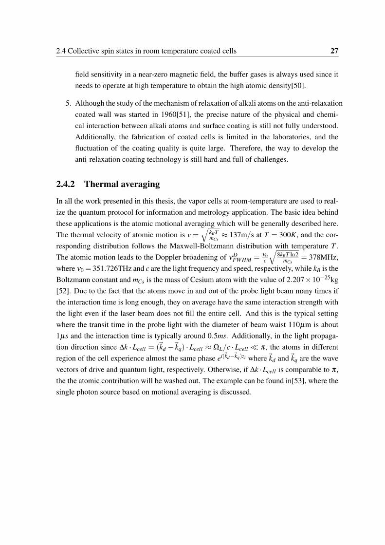
In all the work presented in this thesis, the vapor cells at room-temperature are used to real-ize the quantum protocol for information and metrology application. The basic idea behindthese applications is the atomic motional averaging which will be generally described here.The thermal velocity of atomic motion is v =
√kBTmCs
≈ 137m/s at T = 300K, and the cor-responding distribution follows the Maxwell-Boltzmann distribution with temperature T .The atomic motion leads to the Doppler broadening of νD
FWHM = ν0c
√8kBT ln2
mCs= 378MHz,
where ν0 = 351.726THz and c are the light frequency and speed, respectively, while kB is theBoltzmann constant and mCs is the mass of Cesium atom with the value of 2.207×10⁻²⁵kg[52]. Due to the fact that the atoms move in and out of the probe light beam many times ifthe interaction time is long enough, they on average have the same interaction strength withthe light even if the laser beam does not fill the entire cell. And this is the typical settingwhere the transit time in the probe light with the diameter of beam waist 110µm is about1µs and the interaction time is typically around 0.5ms. Additionally, in the light propaga-tion direction since ∆k · Lcell = (kd − kq) · Lcell ≈ ΩL/c · Lcell ≪ π , the atoms in differentregion of the cell experience almost the same phase ei(kd−kq)zi where kd and kq are the wavevectors of drive and quantum light, respectively. Otherwise, if ∆k ·Lcell is comparable to π ,the the atomic contribution will be washed out. The example can be found in[53], where thesingle photon source based on motional averaging is discussed.


Chapter 3
Experimental system
In this chapter, the experimental setup and measurement methods are presented in detail.The laser system and the corresponding function is discussed at first, which paves the wayfor preparation of initial spin states and probing processing. Then, the key element, micro-cell coupled into an optical cavity, is presented in Section 3.2 where the fabrication pro-cedure is described in order to make the reader easily and intuitively understand the mainresults of this thesis. The general description of optical cavity is followed by another im-portant part, characterization of the quality of our microcells and of optical pumping, which
Fig. 3.1 Main scheme of the experimental setup.
are Faraday angle and magneto optical resonance (MORS) measurement, respectively. The

30 Experimental system
rather long part at the end of this chapter is devoted to the most critical measurement calledquantum noise reconstruction in which measurement method including the calibration also,and the noise contributions from different sources are explained by relating to the theoreticalformula given in previous chapter.
3.1 Laser system
As shown in Figure 3.1, there are totally three laser beams with different optical wavelengthscomposing the laser system in our setup, probe, pump and repump light beams, and the cor-responding laser frequencies are given in Figure 3.2. Pump and repump beams are requiredto prepare the highly orientated spin state as the optical pumping, and the probe light is thebeam interacting with atomic ensembles described in previous chapter.
201MHz
251MHz
9192MHz
F=4F=2F=3F=4
F=5
F=3
F=4
F=3
152MHz
6S1/2
6P3/2
6P1/2
1168MHz
Probelaser
Opticalpumplaser
Repumplaser
D
Fig. 3.2 Level scheme of Cesium and the laser frequencies of probe and optical pumpingbeams.
3.1.1 Probe light
The laser beam from distributed feedback laser TOPTICA DL100 is used as the probe light.Experimentally, the output of the laser is split into two beams after passing through the op-tical isolator, which is used to avoid the potential damage caused by backreflection. Oneof them is used as the main probe beam for the experiment and the other weaker fraction isfor the laser frequency locking. Since we plan to have a large detuning with respect to theD2 transition, a fiber coupled electro optical modulator (EOM) is utilized to generate the

3.1 Laser system 31
upper and lower sidebands at around 1GHz from the carrier frequency. Actually, in orderto achieve the QND picture, typically we use the probe light with a blue detuning around1.6GHz with respect to 6S1/2F = 4 → 6P3/2F ′ = 5 by locking the laser frequency to thesecond blue sideband, which means the relative large modulation depth is required. Theline reflection alignment of the saturation absorption spectroscopy is followed to lock theblue or red sideband to an atomic transition. As shown in the right of Figure 3.3, the p-polarized light beam passes through the polarization beam splitter (PBS), Cs vapor cell, theoptical attenuator and the quarter wave plate, and then is reflected by a 0 high reflectionmirror. Because of the use of the quarter wave plate, the reflected weak signal beam withs-polarization carrying the absorption information is reflected by the PBS, and then hits thelocking detector which provides the error signal for the electronic feedback. Usually, we run
Pro
be
Lig
ht
PBS
DL100
Isola
tor
FF Fiber EOM
HWP QWP
Cs Vapor cell
ND Fileter
HWP
Fig. 3.3 Saturation absorption spectroscopy signal of probe light which corresponds to CsD2 transition line and the experimental scheme of laser frequency locking system with thedetuning of ∼ 1GHz. The black line is the saturation absorption signal and the gray oneshows the error signal for the laser frequency locking.
the experiments in the pulse regime where the temporal profile of the laser beams is gen-erated by means of intensity modulation. For the probe beam an EOM positioned betweentwo PBSs is used as the intensity modulator to create the laser pulse with the duration oforder of several millisecond. By using EOM instead of acoustic optical modulator (AOM),the sharp edges of the pulses including the high frequency components can be prevented.However, when running the experiment in the scheme of stroboscopic modulation, the in-tensity of the probe beam is modulated by AOM at twice the Larmor frequency ∼ 380kHzwith the duty cycle around 15% due to its faster response as an optical switch.

32 Experimental system
3.1.2 Optical pumping
To prepare the highly oriented spin states, optical pumping is usually required[54]. Here theoptical pumping is implemented by sending two circular polarized laser beams to the vaporcell. The pump laser at 894nm with the frequency corresponding to the Cs D1 transition6S1/2F = 4 → 6P1/2F ′ = 4 comes from diode laser DL100 Pro which behaves very wellin terms of frequency stability and shows low frequency noise. And the repump laser at852nm is a homebuild Littrow configuration diode laser and grating stabilized to the CsD2 transition 6S1/2F = 3 → 6P3/2F ′ = 4. The pump and repump laser beam overlappingwith each other share the same propagation direction, parallel to the applied DC magneticfiled direction, and the same circular polarization σ+ or σ− as shown in Figure 3.1. Thepolarization direction of the optical pumping beams partially determines the final populationof atoms. If choosing σ+ polarized beams, the atoms will be populated at F = 4,mF = 4after the optical pumping. Otherwise, the atoms will be populated at F = 4,mF =−4. Theformer is explained in Figure 3.4. For the σ+ pump laser F = 4,mF = 4 is a dark state, andthe atoms in other Zeeman sublevels of ground state 6S1/2F = 4 absorb the σ+ polarizedpump photons and decay towards to F = 4 or F = 3. Due to the fact that σ+ leads to∆mF = +1 transition, finally the atoms still staying in the ground state of F = 4 will bepopulated into F = 4,mF = +4. At the same time, the repump laser collects the atomsdecaying to F = 3 and drives them back to F = 4. Following this logic we can see that the
F=4
F=3
m 1 2 3 4
F=4
F=3
darkstate
(a)
F=4
F=3
F=5F=4
F=3F=2
m 1 2 3 4 5
(b)
Fig. 3.4 The atomic transitions induced by the σ+ polarized pump (a) and repump (b) lightbeam, respectively.
atoms are fully populated into F = 4,mF = 4 after an effective optical pumping process.Notice that since the repump laser is far off resonance to all transitions from the groundstate F = 4, the broadening effect from it is negligible. In the experiment the intensity ofrepump beam can be set strong enough to make sure almost all the atoms go back to theground state F = 4.

3.2 Microcell 33
3.2 Microcell
In this section I will describe the key element of the whole thesis, micro-fabricated Cs vaporcell (microcell) which has experienced at least 3 times evolution on the fabrication. Thecurrent generation of microcell can provide the traverse spin lifetime (T2 time) around 9ms,and the number of atoms about 107 ∼ 108 in a glass cell microchannel with the dimensionof (300µm×300µm×10mm) depending on the environmental temperature. However, cur-rently the light intensity transition through the microcell is not as good as we had expectedwhich limits the degree of spin squeezing and single photon generation efficiency, whichcan be found in Chapter 5 and reference [53], respectively. At present we are struggling toreduce the optical losses by using CO2 laser bonding between bare glass chip and windowswith anti-reflection coating; the local heating can help us to avoid the damage on the coatingsurface.
3.2.1 Fabrication
The first generation of our microcell-chip was designed and fabricated by QUANTOP atNiels Bohr Institute and by Danchip at Danmarks Tekniske Universitet. Photos of cells are
10m
m 8mm
2mm
(b) Microcell sealed inside glass container. (a) 4-layers glass-silicon chip.
(c) laser bonding of windows.
Fig. 3.5 Photos of the first generation Cs vapor microcell.
shown in Figure 3.5. A chip is made of 4 layers of glass and silicon joined together throughanodic bonding, and the microchannel with a 200µm×200µm cross section was developedon the middle glass layer by Micro saw. More complicated procedure was implemented

34 Experimental system
when fabricating the holes in the silicon layer with the size of 20 ∼ 54µm for the injectionof atomic vapor gas and anti-relaxation coating material. Details can be found in Appendix2. Since two different materials were used to form the cell-chip, laser bonding betweenthe chip and windows with anti-reflection coating layer did not work (see Figure 3.5(c)).Therefore, we decided to replace this 4-layer cell-chip with a single piece of glass chip.
(a) Bare chip (no windows) with microchannel.
(b) Closeup of microchannel and laser-drilled microhole.
(c) Finished microcell with windows.
Fig. 3.6 Photos of the current Cs vapor microcell.
The current version of mircocell is shown in Figure 3.6, where microcell-chip is basedon the borosilicate glass slab from VitroCom containing a microchannel with the cross-section of 300µm×300µm. A microhole (∼ 20µm) is laser drilled on one of the microcell’ssurfaces to allow atoms to enter, and the surfaces of the glass chip are super-polished inorder to avoid any air gaps. Although the current microcell is encapsulated in a cylinderglass container where the windows are attached by mechanical pressure, we are developingthe glass-to-glass laser-bonding procedure in our lab to attach windows at the edges of thecell, and attach a round tube to the cell’s top surface where the micro-hole sits. Note that inthe fabrication of the current microcells the annealing procedure at 550 for the whole glassstructure is implemented to remove stresses that the fusing process may have caused.
As mentioned at the end of previous chapter, since thermal atoms confined in a con-tainer will lose their spin orientation information after colliding with the bare glass walls,the anti-relaxation coating, Alkene C20, is deposited on the inner surface of the microcellsby Misha Balabas, an coating expert from S. I. Vavilov State Optical Institute in Russia. Inthe first generation of microcell based on 4-layer silicon-glass chips, the typical spin depop-

3.2 Microcell 35
ulation time T1 (also called longitude spin decoherence time) is 1 ∼ 2ms, correspondingto ∼ 3000 times of bounces which is lower than the value we expected according to the
Cell No. 1 2 3 4 5 6Volume[µl] 60 18 24 26 13 80Radius[cm] 0.24 0.16 0.179 0.184 0.146 0.267
T1[ms] 200 54 95 75 60 80Nb[×103] 13.3 5.4 8.6 6.6 6.6 4.8
Table 3.1 Number of bounce with 140 Alkene C20 coating.
coating performance on the macro-spherical vapor cells. When we switched to the currenttype of microcell based on the chip of borosilicate glass where the smooth channel surfaceis better for alkene coating deposition, we spent some time on investigating the coatingcondition. We made two batches of spherical vapor cells with different coating depositiontemperatures (140 and 280) since we thought the typical coating temperature (140) wasnot sufficient to form the even distribution and thick enough coating layer. The correspond-ing results are shown in Table 3.1 and Table 3.2, and it is proved that the higher coatingdeposition temperature can really improve the coating quality. By looking into Table 3.2where six spherical vapor cells with different sizes were involved in the test, it is found that
Cell No. 1 2 3 4 5 6Volume[µl] 12 28 62 500 1800 4200Radius[cm] 0.14 0.19 0.25 0.5 0.75 1
T1[ms] 110 207 336 220 1093 1382Nb[×103] 12.64 17.77 22.33 7.230 23.48 22.33Table 3.2 Number of bounce with 280 Alkene C20 coating.
the number of bounce keeps increasing when the size is very small, then achieves a constantvalue ∼ 2.3× 10⁴ except the abnormal one No.4. This can be explained in the followingway. There are two different main mechanisms limiting the spin lifetime of atoms insideof the cell, one is from wall collision and the other is the leakage of the atoms from anyholes which is determined by the ratio of hole size to the volume of the entire cell. Allthe cells almost have the gaps with the same size, thus it is very obvious when the leakagecontribution is comparable to the wall collision contribution ( in other words, the volume isquite small). This coating temperature then was used to fabricate the current microcells andresulted in a much better performance than before, the dark T1 time is of ∼ 17ms and darkT2 time ∼ 9ms. The measurement procedure for T1 and T2 is described in Section 3.2.2 and3.2.3 below.

36 Experimental system
The main limitation for the current microcell is the light power transmission, which is∼ 90% now even if the good anti-reflection coated windows are attached, which poses somelimitations for our experiments that will be discussed later. It could be from the coatingdamage when the pressure is applied to attach the windows, therefore, we are running thelaser bonding procedure to attach the windows at the edges of the cell, and attach a roundtube to the cell’s top surface where the micro-hole is drilled.
3.2.2 Faraday angle
Faraday rotation measurement is one of the important test to characterize the quality ofthe vapor cells, which can determine the collective spin component in light propagationdirection, and if the atomic ensemble is highly polarized the atomic density can be deducedfor this measurement. Additionally, the evolution of Faraday angle can tell us the spindepolarization time due to the fact of
θF(t) =−Γλ 2 ⟨Jx⟩(t) ·a1(∆)
16A∆2π(3.1)
where λ = 852nm and Γ = 2π · 5.21MHz are the wavelength of the probe light and thefull width at half maximum (FWHM) linewidth of the excited state, respectively, while⟨Jx⟩(t) = ⟨Jx⟩(0)e−t/T1 . For this measurement we are probing in the x-direction. We assumea fully oriented sample here, which means in the experiment one should make sure that theoptical pumping is effective by checking the polarization and light intensity of pump andrepump beams to maximize the Faraday angle appearing directly in the oscilloscope, thenone can get the initial Faraday angle value as follow
θF ≈−Γλ 24Naa1
16A∆2π≈−Γλ 24ρa1L
16∆2π(3.2)
where ρ is the atomic density, while A and L are the area and length of the cell, respectively.It is found in Equation 3.2 that the Faraday angle is only proportional to the sample lengthwith a given atomic density. Therefore, we send all three beams in the same directionparallel to the bias DC magnetic field, as shown in Figure 3.7. For the data presented inthis section, beam pulses were created with a chopper and shutter. The pulse sequencewas ∼ 50ms of combined pump/repump beam, followed by ∼ 50ms of probe beam. Thestatic magnetic field was produced using a small ring magnet placed next to the microcell.We have since replaced the chopper with AOMs to create cleaner pulses. In addition, wehave removed the magnet and instead installed a 3-layer µ metal shield containing DCcoils around the microcell to generated a more homogenous bias magnetic field. Depending

3.2 Microcell 37
Probe light
λ/2 λ/4 Microcell
BS
Oscilloscope
Det 1
Det 2
PBS
Magnetic Ring
B
BS
Repump light
Pump light
λ/2 λ/4
λ/2
Pulse sequence
repump
probe
Shutter
t=0
Fig. 3.7 Faraday rotation measurement.
0 5 10 15 20 25 30 35 40 450
0.2
0.4
0.6
0.8
1
1.2
1.4
1.6
1.8
t[ms]
Fara
day
angl
e [d
egre
e]
Experimental data
θF
=1.577(4)°exp(−x[ms]/17.69(15)[ms])+0.008(5) °
(a)
0 200 400 600 800 10000.02
0.04
0.06
0.08
0.1
0.12
0.14
0.16
0.18
0.2
Probe power[nW]
1/T 1[m
s]
1/T1
T −11
=0.04(4)[ms −1]
+0.00015(7)[(ms× nW) −1]*P[nW]
(b)
Fig. 3.8 Results of Faraday rotation with ∆ = 850MHz. (a) shows the Faraday rotationevolution during the probing process, and (b) presents the values of 1
T1with different probe
power where the dark T1 time can be extrapolated from the linear fitting.

38 Experimental system
on the room temperature the Faraday angle varies between 1.5 and 2.4, and the averagenumber of atoms is ∼ 107 (see Figure 3.8).
3.2.3 T1 and T2
In general, we use two different decay constants to characterize the coherence of collectivespin, T1 and T2. T1 is the decay of classical mean value Jx in our experiment, and calledspin depolarization time describing the reduction of vector length. Population transfer intoF = 3 whose contribution to the Faraday rotation is negligible, and population also transferinto other magnetic sublevels F = 4,mF = 3,2 whose Faraday rotation contributions arereduced in a factor of 3/4 and 1/2, cause the decay of Jx when starting from the fullyoriented state. Although Faraday rotation measurement has been used to measure the atomicdensity and also T1 time as explained in last section, here I will introduce another methodto characterize this T1 time again which is more convenient once the microcell is coupledinto the optical cavity and well aligned. The experimental setup is shown in Figure 3.1, andthe corresponding pulse sequence is shown in Figure 3.9(a). The optical pumping polarizes
Optical
Pumping 2nd Probe t 1st
Probe
Brf
Optical
Pumping Probe t Brf
(a) Pulse sequence of T1 measurement
(b) Pulse sequence of T2 measurement
Fig. 3.9 Experimental pulse sequence for T1 and T2 measurement. The durations of opticalpumping and RF pulses are 5ms and 200µs, respectively.
almost all the atoms into F = 4,mF = 4 initially with the spin orientation above 98% (thecorresponding characterization will be discussed later.). When the probe light is switchedon, the decay of ⟨Jx⟩ gets faster than the decay in the dark due to spontaneous emission fromthe probe. Then a RF pulse that creates an excitation of ∆mF = 1 when the frequency is onresonance with Larmor frequency ΩL is followed by the second probe pulse to measure thatspin response which is proportional to the mean value of Jx[55]. Given a fixed probe power,
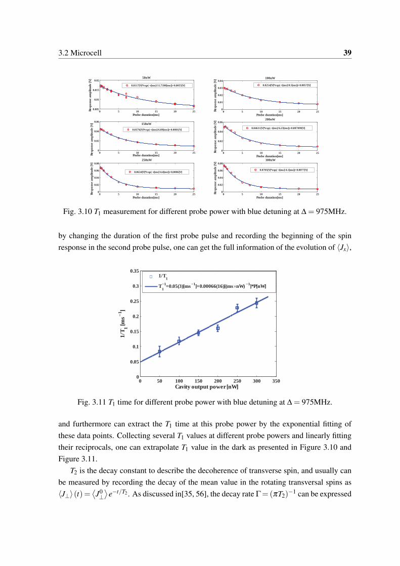
3.2 Microcell 39
0 5 10 15 20 250.005
0.01
0.015
0.02
Probe duration[ms]
Resp
onse
am
plitu
de [V
] 50nW
0.0117[V]*exp(−t[ms]/11.7398[ms])+0.0055[V]
0 5 10 15 20 250
0.01
0.02
0.03
0.04
Probe duration[ms]
Resp
onse
am
plitu
de [V
] 100nW
0.0254[V]*exp(−t[ms]/8.5[ms])+0.0057[V]
0 5 10 15 20 250
0.02
0.04
0.06
Probe duration[ms]Resp
onse
am
plitu
de [V
] 150nW
0.0376[V]*exp(−t[ms]/6.89[ms])+0.0081[V]
0 5 10 15 20 250
0.02
0.04
0.06
Probe duration[ms]
Resp
onse
am
plitu
de [V
] 200nW
0.04611[V]*exp(−t[ms]/6.23[ms])+0.007099[V]
0 5 10 15 20 250
0.02
0.04
0.06
0.08
Probe duration[ms]
Resp
onse
am
plitu
de [V
]
250nW
0.0634[V]*exp(−t[ms]/4.4[ms])+0.0086[V]
0 5 10 15 20 250
0.02
0.04
0.06
0.08
Probe duration[ms]
Resp
onse
am
plitu
de [V
] 300nW
0.0705[V]*exp(−t[ms]/4.1[ms])+0.0077[V]
Fig. 3.10 T1 measurement for different probe power with blue detuning at ∆ = 975MHz.
by changing the duration of the first probe pulse and recording the beginning of the spinresponse in the second probe pulse, one can get the full information of the evolution of ⟨Jx⟩,
0 50 100 150 200 250 300 3500
0.05
0.1
0.15
0.2
0.25
0.3
0.35
Cavity output power [nW]
1/T 1 [m
s−1]
1/T
1
T1−1=0.05(3)[ms −1]+0.00066(16)[(ms× nW) −1]*P[nW]
Fig. 3.11 T1 time for different probe power with blue detuning at ∆ = 975MHz.
and furthermore can extract the T1 time at this probe power by the exponential fitting ofthese data points. Collecting several T1 values at different probe powers and linearly fittingtheir reciprocals, one can extrapolate T1 value in the dark as presented in Figure 3.10 andFigure 3.11.
T2 is the decay constant to describe the decoherence of transverse spin, and usually canbe measured by recording the decay of the mean value in the rotating transversal spins as⟨J⊥⟩(t) =
⟨J0⊥⟩
e−t/T2 . As discussed in[35, 56], the decay rate Γ= (πT2)−1 can be expressed

40 Experimental system
as follow,Γ = a+b ·θF + c ·P+d ·P2 + e · (θFP). (3.3)
The combination of the first two terms contributes to the decay rate in the dark, where
0 100 200 300 400 500 600 7000
0.1
0.2
0.3
0.4
0.5
0.6
0.7
Cavity output power [nW]
T2−1
[ms−1
]
1/T2
T2−1=0.096(19)[ms−1]+0.00075(5)[(ms× nW) −1]*P[nW]
Fig. 3.12 1/T2 for different probe powers with blue detuning ∆ = 1.598GHz. T2 time in thedark can be extrapolated from the linear fitting which gives the value of about 10ms.
the constant a is from the wall collisions, losses due to atom leaving the effective cell vol-ume to other part (e.g. the stem), and the magnetic field instabilities and inhomogeneity.The second term proportional to atom number θF ∝ Na comes mainly from the collisionsbetween atoms. The spontaneous emission induced by the probe light is embodied in theterm involving probe power P only, while the quadratic part in probe power probably resultsfrom the inhomogeneous intensity distribution of the light which causes atoms to experi-ence different Stark shifts in different regions of the cell. The last term in Equation 3.3 isrelated to the higher order coherent interaction between light and atoms, and is called γswap
in Equation 2.38 in order to be distinguished from the incoherent decay. In the experimentfor T2 estimation, we keep the setup as in Figure 3.1 but with a different pulse sequencefrom T1 measurement that is shown in Figure 3.9(b). Since we mainly concentrate on theQND picture in the work of this thesis, probe light with the blue detuning of ∆ = 1.598GHzis used to measure the T2 time where the effect from the tensor interaction is very small andcan be neglected according to Figure 2.17. The corresponding result is presented in Figure3.12.

3.3 Optical cavity 41
3.3 Optical cavity
Optical cavity is one of the widely used elements in physical research, which can enhancethe interaction between light and matter[57, 58, 59], modify the spatial and spectral modesof light fields[60], provide phase feedback[61, 62]. In our setup shown in Figure 3.1, theoptical depth in the atomic ensemble is enhanced by coupling the microcell into the funda-mental mode of a standing wave cavity. This section is devoted to the general descriptionof optical resonator and the related technologies. Let us consider a simple model of stand-ing wave cavity with input and output concave mirrors M1 and M2. The correspondingcurvatures are r1 and r2, respectively. In our experiment, because of the large diameter ofmagnetic shield a near concentric cavity is built with the curvature of r1 = r2 = 110mm. Byusing the method of equivalent confocal cavity[63], we can derive the formula about beamwaist and beam size w0 at the end mirrors w1,2 as follow,
w0 =
√f λ
π,
f 2 =L(r−L)(r−L)(r+ r−L)
((L−R)+(L−R))2 ,
w1 = w2 =
√λLπ
(r2 × (r−L)
L(r−L)(r+ r−L))1/4,
(3.4)
where f is the equivalent focal length. Figure 3.13 shows the dependence of these param-eters on cavity length in our setup. At present we choose the cavity length as 218mm with
215 216 217 218 219 2200
102030405060
Radius @mmD
Wai
stra
dius
@Μm
D
(a)
215 216 217 218 219 220
500
600
700
800
900
Radius @mmD
Bea
mat
cavi
tym
irro
r@Μ
mD
(b)
Fig. 3.13 Dependence of beam size on the cavity length. (a) shows the beam waist radius atdifferent cavity length, and (b) shows the beam diameters on the end mirrors.
the beam waist of 110µm in diameter which is an optimal value for the interaction, a good

42 Experimental system
compromise between low clipping losses and good filling factor. And also with the consid-eration that the cavity mirrors are set out of the cylindrical magnetic shield whose diameteris 190mm.
Let us look at the cavity properties in the frequency domain. Given the intensity reflec-tivity of input and output mirrors as R1 and R2, and the round trip intracavity loss as lcav,one can derive the formula for the finesse F as follow[64],
F=ν f ree
∆ν=
π√
gm
1−gm,(gm =
√R1 ·R2(1− lcav)) (3.5)
where ν f ree is the free spectral range (FSR) and ∆ν is the cavity bandwidth, while gm givesthe amplitude reduction of the internal field during each round trip. If we introduce thephase difference for each trip as δφ = 2π(νL −νcav) ·2L/c with the laser frequency νL andthe eigenfrequency of cavity mode νcav, the total effect of cavity during one round trip canbe described by g(ν) = gme−iδφ . Therefore, the power spectrum of transmitted light andreflected light can be obtained as
Pout =(1−R1)(1−R2) |g(ν)|√
R1R2 |1−g(ν)|2Pin,
Pre f =|R1 −g(ν)|2
R1 |1−g(ν)|Pin
(3.6)
In Figure 3.14, the calculated power spectrums of both transmitted and reflected light aregiven under the experimental condition of R1 = 99.7% and R2 = 80% with the round triploss of 13.3%, and the reason of choosing those values will be explained in Chapter 5 aboutconditional spin squeezing.
2 ´ 109 4 ´ 109 6 ´ 109 8 ´ 109 1 ´ 10100.000
0.005
0.010
0.015
0.020
Frequency @HzD
Pow
ersp
ectr
umof
tran
smitt
edlig
ht
(a)
2 ´ 109 4 ´ 109 6 ´ 109 8 ´ 109 1 ´ 10100.90
0.92
0.94
0.96
0.98
1.00
Frequency @HzD
Pow
ersp
ectr
umof
tran
smitt
edlig
ht
(b)
Fig. 3.14 Calculated power spectrum of transmitted(a) and reflected(b) light that have beennormalized to the input power.

3.4 Preparation and characterization of the atomic state 43
Experimentally, the optical cavity is frequency locked on resonance by a Pound-Drever-Hall technique[65]. Instead of the MHz phase modulation on the input light field, a 10kHzmodulation is applied on the piezoelectric transducer (PIZZOMECHANIK GmbH)since thebroad bandwidth of the cavity ( about 40MHz ) makes the phase modulation difficult. Anddetails of frequency locking technology can be found in Appendix3.
3.4 Preparation and characterization of the atomic state
As mentioned above, optical pumping is employed to create the highly oriented spin stateswhich is quite important in the interface between light and atoms. The circular polarizedpump and repump beams, corresponding to Cs D1 and D2 transitions respectively, are sentto the vapor cell parallel to the DC magnetic field which creates the Zeeman splitting as thequantization axis. In order to verify the atomic CSS state, an RF magnetic field is employedto excite the coherent transition between different magnetic sublevels that can be read outby the probe light. This is called magneto optical resonance signal (MORS).
3.4.1 Magneto optical resonance
The MORS experiment can be run in frequency or time domain which shares the same setupas Figure 3.1. In this section I only shows the experiment in the time domain where thelinewidth broadening from the pump beam is avoided. And MORS experiment in frequencydomain can be found in[31, 34, 35]. The interaction of atoms with a magnetic field isdescribed by the Hamiltonian which has been used in Chapter 2 when deriving the input-output formula in rotating frame
Hmag = gF µFJ ·B+O(B2), (3.7)
where µB is the total angular momentum of the atom. Notice that the second term inEquation 3.7 describes the higher order effect from the magnetic field which behaves ap-proximately as the quadratic Zeeman frequency difference between σm,m+1 and σm−1,m asνqz ≈ 2ΩL
νh f swith the hyperfine splitting of the Cesium ground state νh f s = 9.1926GHz. In the
experiment, a DC bias magnetic field Bx induces the Larmor procession at ΩL = gF µFBx/h,and also the quadratic Zeeman splitting. Additionally, if an RF magnetic field at frequencyΩ along the z-direction is added, the transverse spin components in the rotating frame can

44 Experimental system
be written as
∂ J′y∂ t
=−ωc cos(ΩLt)cos(Ωt +φ)Jx,∂ J′z∂ t
=−ωs sin(ΩLt)sin(Ωt +φ)Jx, (3.8)
with the Rabi frequency ωc,s = gF µFBc,s/h where Bc,s is the amplitude of the RF cosine andsine components. When the RF magnetic field is on resonance so that Ω = ΩL and settingφ = 0, the above formula with the assumption of long interaction time ωcT,ωsT ≪ 1 ≪ ΩTcan be rewritten as
∂ J′y∂ t
=−ωcJx
2,
∂ J′z∂ t
=−ωsJx
2. (3.9)
Hence, a displacement in the rotating frame is created by the resonant RF magnetic fieldwhich represents an excitation of all ∆m = 1 coherence and can be mapped onto the probelight through the interaction between light and atoms. By using Equation 2.25 and 2.33 wecan get the MORS signal in frequency domain as
MORS(Ω) =
√⟨xout
c ⟩2 + ⟨xouts ⟩2
∝
∣∣∣∣∣Na
F−1
∑m=F
F(F +1)−m(m+1)i(Ωm+1,m −Ω)−Γm+1,m/2
⟨σm+1,m+1 − σm,m
⟩∣∣∣∣∣ , (3.10)
where Γm+1,m are the FWHM linewidths of each coherence and Ωm+1,m are the individualcoherence evolution frequencies, while the measured light components
⟨xout
c,s⟩
∝⟨Jin
y,z⟩. This
formula is the Fourier transformation of MORS signal in time domain
MORS(t) ∝
∣∣∣∣∣Na
F−1
∑m=F
[F(F +1)−m(m+1)]eiΩm+1,mte−Γm+1,mt/2 ⟨σm+1,m+1 − σm,m
⟩∣∣∣∣∣ .(3.11)
Experimentally, a Larmor precession at frequency Ω = 698kHz is induced by the DC biasmagnetic field (∼ 2Gauss), and the corresponding quadratic Zeeman splitting is 105Hzwhich allows us to resolve all the eight Lorentzian peaks with the weak probe beam. Thepulse sequence is same as that in T2 measurement, and a 100ms weak probe light pulse isused to guarantee the sufficient frequency resolution. Figure 3.15 and 3.16, show the par-tial and highly polarized MORS signals, respectively, where only repump light is employedin the former case and the complete optical pumping is used in the latter case. Note thatthe left graphs of these two figures present the detected signal in time domain where thebeating comes from the coherent excitations in different magnetic sublevels. And the spin

3.4 Preparation and characterization of the atomic state 45
0 20 40 60 80 100−1
−0.5
0
0.5
1
time [ms]
sign
al [a
.u.]
XYRR t
(a)
−800 −600 −400 −200 0 200 400 600 8000
0.05
0.1
0.15
0.2
0.25
frequency [Hz]
sign
al [a
.u.]
measured datascaled t(zero padded date)t
(b)
Fig. 3.15 Pulsed MORS signal for an optical pumping cycle resulting in the 76% spin ori-entation when only the repump light is on.
0 20 40 60 80 100−0.5
0
0.5
time [ms]
sign
al [a
.u.]
XYR
(a)
-1500 -1000 -500 0 500 1000 1500f @HzD
0.2
0.4
0.6
0.8
1.0
R
(b)
Fig. 3.16 Pulsed MORS signal for an optical pumping cycle resulting in the 98.5% spinorientation when both pump and repump light are on.

46 Experimental system
orientation is defined as
pF=4 =14
4
∑m=−4
mσm,m (3.12)
In general, the splitting between the peaks is determined by not only the quadratic Zeemanshift νqz but also quadratic Stark shift νqs which is given by[31]
νqs[Hz] =−Γλ 2a2(∆)
16π2A∆Φ(t)[1+3cos(2α)]
= 1.03×10⁶HzP[mW]a2(∆)
A[cm2]∆blue(MHz)[1+3cos(2α)],
(3.13)
where α is the angle between the macroscopic spin direction (the x-axis) and the probepolarization direction. As shown in Equation 3.13, the quadratic Stark shift is related to the
-3 -2 -1 0 1 2 3
-20
0
20
40
60
Α@radD
Qua
drat
icS
tark
shif
t@H
zD
(a) ∆blue = 850MHz.
-3 -2 -1 0 1 2 3
-10
-5
0
5
10
15
20
Α@radD
Qua
drat
icS
tark
shif
t@H
zD
(b) ∆blue = 1.6GHz.
Fig. 3.17 Quadratic Stark shifts for different polarization direction of probe light.
0.0 0.5 1.0 1.5 2.00
2
4
6
8
10
Probe Power@ΜWD
Qua
drat
icSt
ark
Shif
t@HzD
Fig. 3.18 Quadratic Stark shift for different probe power with blue detuning ∆ = 1.6GHzand y-direction linear polarization.
laser detuning ,polarization direction and intensity of the probe light. Figure 3.17 shows theshift evolution with different polarization direction at ∆blue = 850MHz and ∆blue = 1.6GHz.

3.5 Coupling strength 47
Figure 3.18 gives the quadratic Stark shift for different probe powers at ∆blue = 1.6GHz.Since in the MORS experiment we use the probe beam with the intracavity power of 0.5µWand the detuning is ∆blue = 1.6GHz, this effect is negligible and the quadratic Zeeman effectis the dominant contribution to the splitting of the peaks.
3.5 Coupling strength
In this section I will introduce one of the key parameters in our experiment, the couplingstrength κ . In the QND scenario mentioned in Chapter 2, this dimensionless constant canbe represented as κ2 = a2 · SxJxT ∝ NaNph where Na and Nph are the number of atomsand photons respectively. Although only QND interaction is discussed in this thesis, thedefinitions for different scenarios can be found in[35]. There are two typical methods beingused to find this constant, one is to transfer a known displacement of coherent light stateto the atoms and then read out this coherent displacement of the atomic state[32], and theother method relies on the noise measurement of thermal atomic state[35]. The formercalled mean value transfer is quite useful, especially when calibrating the coupling strengthin the non-QND picture where swapping interaction is included, but in the following I amfocusing on the latter one.
Atomic spins in thermal equilibrium, that is the unpolarized spin state, are not affectedby the higher order interaction. In the thermal state, it is fully symmetric which meansj2x = j2
y = j2z = F(F+1)
3 = 203 . In this setting all atomic sublevels have the same population;
the same gose for atoms in F = 3 manifold which are not observed in the measurement.Since there are 16 sublevels totally and 9 of which belong to F = 4, the observed spin noisewill thus be Na
203 · 9
16 = 154 Na. This is a factor of 15
8 comparing with the atomic noise inthe CSS state which is FNa/2 = 2Na. Therefore, the observed spin noise in the thermalstate should be 15
8 ·Var(xA(pA))CSS. Since in the thermal spin state the mean value of vectorjx equals to zero which leads to the fact that the enhancement from Jx of coupling thelight variables to the atomic spin variables is negligible, the backaction of light on itselfdisappears. By looking at Equation 2.25, the corresponding input-output relation in termsof Stokes vectors can be read as
Souty(c,s) = Sin
y(c,s)+aSxT
2Jz,y
= Siny(c,s)+
κ√
SxT2√
JJz,y,
(3.14)
where J = 4Na for hyperfine level F = 4. In the derivation from the first line to the second

48 Experimental system
line I use the fact that κ = a√
SxJT and in the CSS state Jx = J = 4Na as mentioned before.If calculating the noise of the measured light variable Sy(c,s), we can get
Var(Souty(c,s)) =Var(Sin
y(c,s))+κ2SxT
4JVar(Jz,y). (3.15)
Let us use some knowledge about light noise which I will show in the next section. As-suming the input light is in the coherent state ( or called shot noise limited), the noise ofVar(Sin
y(c,s)) is defined as Var(Siny(c,s)) =
SxT2 =
Nph4 . Thus, Equation 3.15 can be rewritten as
Var(Souty(c,s))thermal =
SxT2
[1+κ2
2Var(
Jz,y√J)]
=SxT
2[1+
κ2
2158].
(3.16)
Furthermore, the coupling constant can be derived from the measured light noise Var(Souty(c,s))
as
κ2 =
Var(Souty(c,s))thermal
SxT2
−1
15/16
=σ2
thermalSN −115/16
,
(3.17)
where σ2thermalSN means the measured noise of the output light has been normalized into
Probe pulse Probe pulse Probe pulse t
33ms
Fig. 3.19 Pulse sequence for the thermal noise measurement.
the shot noise unit. It is a good way to extract κ in the QND scenario from the noisemeasurement of atomic spins in the thermal equilibrium where laser detuning ∆blue is muchlarger than the hyperfine splitting of the excited states so that the tensor interaction is signifi-cantly suppressed. However, when swap operation is included the coupling constant κthermal
slightly differs from κ =√
γsγ
√1−e−2γT
ζinvolved in the real interaction. More details can be
found in[35].Figure 3.19 shows the pulse sequence for the thermal noise measurement where we
choose the laser detuning as ∆blue = 1.6GHZ so that the role of tensor interaction can beneglected as discussed in Chapter 2. The time gap between two probe pulses is usually set to

3.6 Quantum noise 49
0 2 4 6 8
x 107
0
0.5
1
1.5
Number of Atom
κ2 from
ther
mal
noi
se m
esur
emen
t
Fig. 3.20 κ2 extracted from the thermal noise measurement for different numbers of atoms.Interaction time and laser detuning are 0.5ms and ∆blue = 1.6GHZ, respectively.
33ms to ensure the fully thermalization of atoms even if the probe beam has some pumpingeffect. Figure 3.20 and Figure 3.26(shown in next section) present the dependence of κ2 onthe number of atoms and photons, respectively. In order not to confuse the readers I shouldmention the way to change the number of atoms here. Previously, the number of atomswas changed by tuning the environment temperature inside the magnetic shield, however,the range is very limited, typically from 17C to 30C since only air heating process wasemployed but no cooling. In the procedure of measuring the data involved in Figure3.20,heating process is still kept but instead of air heating, a twisted wire with high resistanceis wound around the aluminum cylinder where most of the magnetic coils are attached. Byadding the current on this wire the stable environment temperature can be established insidethe cylinder. We can decrease the number of atoms by weakening the repump beam butkeeping the same intensity of pump beam to reduce the number of atoms in the F = 4. Inthis scheme, the number of atoms is calibrated against a response to a RF field.
3.6 Quantum noise
3.6.1 Light noise
Before describing the quantum noise measurement, I would like briefly to remind the readersabout our detection system. Since the drive light or probe light is used as the strong localoscillator which shares the same phase as the generated quantum light and the polarizationof the local oscillator light is orthogonal to that of the quantum beam as shown in Chapter 2,polarimetric measurement of light, also called polarization homodyne detection is employed

50 Experimental system
in our system which is in principle a typical balanced homodyne detection of light[64]. Thecorresponding schemes of Sy and Sz components are shown in Figure 3.21.
x
y z
HWPθ=π/4
−
PBS
(a) Sy measurement
QWPθ=π/4
−
PBS
(b) Sz measurement
HWPθ=0
Fig. 3.21 Detector systems for measuring the Sy and Sz components,respectively. HWP:half-wave plate; QWP: quarter-wave plate; PBS: polarization beam splitter. θ is the anglebetween the polarization direction of light and the optical axis of waveplate.
x
y z
HWPθ=π/4
−
PBS
LocalSignal
BS d1
d2
PZT
Fig. 3.22 Homodyne detection scheme. BS: 50/50 beam splitter
Figure 3.22 gives the typical homodyne detection scheme. Assuming the phase differ-ence between the local oscillator L and the signal beam a is φ , and the output mode fromthe beam splitter can be written as
d1 =1√2(a− Leiφ ), d2 =
1√2(a+ Leiφ ). (3.18)
In the traditional scheme, the relative phase difference is controlled experimentally by themovement of piezoelectric ceramic which is connected to the high reflected mirror. The

3.6 Quantum noise 51
photocurrents detected by two separated low noise detector with high gain are given as:
id1 = d†1 d1 =
12(a†a− a†Leiφ − aL†e−iφ + L†L),
id2 = d†2 d2 =
12(a†a+ a†Leiφ + aL†e−iφ + L†L), ,
(3.19)
By linearization, which means the operator can be described by a classical component anda quantum noise operator, i.e. a = α + δ a and L = l + δ L, we can get the difference ofphotocurrents
i− = id1 − id2 = a†Leiφ + aL†e−iφ
= α∗leiφ +αl∗e−iφ +α
∗δLeiφ +αδL†e−iφ + lδ a†eiφ + l∗δ ae−iφ .
(3.20)
Since in the experiment the intensity of local oscillator is much stronger than that of signalbeam, i. e. l ≫α and assuming l = l∗, the third and fourth terms are negligible and Equation3.20 can be simplified as
i− = α∗leiφ +αle−iφ + lδ a†eiφ + lδ ae−iφ , (3.21)
where the fluctuation part of the difference of photocurrents is
δ i− = lδ a†eiφ + lδ ae−iφ , (3.22)
Therefore, when φ = 0 δ i− = lδXs which is the quantum fluctuation of the amplitudequadrature, while when φ = π/2 δ i− = lδPs corresponding to the quantum fluctuation ofthe phase quadrature. When the signal beam is replaced by the vacuum input, the quantumfluctuation is
δ i− = lδV †eiφ + lδV e−iφ , (3.23)
which corresponds to the shot noise limit no matter which phase different one chooses.
In the polarization homodyne detection, by inserting a half-wave plate (HWP) in front ofthe polarization beam splitter (PBS), the light is split into 45 and −45 modes in the outputports of PBS (φ = 0)and then directed into two photodiodes of ultra-low noise differentialAC-coupled photodetector whose performance can be found in[66]. The measurement of thedifferential power of these two modes corresponds to the measurement of the Sy component.If we insert a quarter-wave plate (QWP) or a combination of HWP and QWP (φ = π/2),the differential power of σ+ and σ− modes can be detected which is the measurementof Sz component. Figure 3.23 shows the dependence of photon shot noise on the input

52 Experimental system
probe power, and the linearity demonstrates the behavior of photon shot noise limit sincefor the coherent state of light the variances of Sy and Sz should satisfy the condition ofVar(Sy) = Var(Sz) =
Sx2 =
Nph4 . I should mention that the data shown in Figure 3.23 were
0 0.5 1 1.50
2000
4000
6000
8000
10000
12000
14000
Probe power [µ W]
Phot
on n
oise
[µ V
2 ]
PN[ µ V 2] = 9.2e+003[µ V 2/µ W]*P[ µ W] +34 µ V 2
Fig. 3.23 Measured photon shot noise with different input light power.
taken by injecting the light beam into the detector directly without passing through thecavity and microcell. However, during the glass blowing phase in the fabrication of thenew batch of microcell (Generation D and E), the effect of birefringence induced by intra-stress gets obvious. Although in the fabrication of Generation E an annealing process wasimplemented, this effect is not fully canceled which is shown in Figure 3.24. It can beexplained in the following way. The cavity input linear polarized beam can be seen as acombination of σ+ and σ− circular polarized beam with a fixed phase difference. Insidethe cavity these two modes experience fixed different phases when passing through the glasscylinder. However, the frequency fluctuation makes this phase difference random and withsome uncertainty. Therefore, the output beam composed of these two circular polarizedmodes has the polarization uncertainty or called polarization noise.
3.6.2 Reconstruction of the atomic spin noise
Since the atomic observable cannot be measured directly in an easy way, the interactionbetween light and atoms is utilized to do the atomic state tomography where the informationof atomic spins is mapped onto the light field which serves as quantum bus, and then readout by means of the detection of light.
In the QND picture we have derived the input-output relations for the light and atoms asEquation 2.31, and the corresponding quantum variances for the measured light observable

3.6 Quantum noise 53
0 100 200 300 400 500 600 700−1
0
1
2
3
4
5x 10
−6
Average probe power [nW]
Ligh
t noi
se [V
2 ]
y = 5.5e−009*x − 1.2e−007y = 4.1e−012*x 2 + 2.9e−009*x + 1.2e−007
Light Noise linear quadratic
Fig. 3.24 Measured photon noise with different light power when Microcell E4 is coupledinto the optical cavity.
can be given as follows(Var(xout
c )
Var(xouts )
)=
(Var(xin
c )
Var(xins )
)+
κ2
2
(Var(pin
A )
Var(xinA )
)+
κ4
16
(Var(pin
s )
Var(pinc )
),
+κ4
48
(Var(pins,1)
Var(pin,c,1)
) (3.24)
Assuming the collective spin state of an atomic ensemble is prepared in CSS state whichgives Var(xin
A )=Var(pinA )=
12 , and the light field is shot noise limited, which means Var(xin
c,s)=
Var(pinc,s) =
12 and Var(pin
c,1) =Var(pins,1) =
12 , Equation 3.24 can be simplified to
Var(xoutc(s)) =
12[1+κ
2/2+κ4/12]. (3.25)
Physically, the first term is the shot noise of the probe light, the second term describes thespin noise, and the last term is from the quantum backaction noise of the measurement. Inthe experiment, the time-integrated homodyne signal is scaled by the shot noise of the light.Figure 3.25 shows the measured noise of xout
c,s where the falling mode function e−γT withγ = 1/T2 has been used as mentioned in Chapter 2. The quadratic dependence of measurednoise on the probe power is partially from the backaction contribution shown in Equation3.25 since κ2 ∝ Nph as well as the spontaneous emission. To understand Equation 3.25, themeasured noise from the output light σ2
measured(Souty ) is firstly normalized into the shot noise
unit as Var(xoutc(s)) =
σ2measured−σ2
ENσ2
lightraw−σ2EN
where σ2EN is the noise floor coming from the measurement
apparatus or called electronic noise, and the corresponding data are shown in Figure 3.26.As discussed above, the coupling strength κ2 is proportional to the photon number or probe

54 Experimental system
100 200 300 400 500 600 700 800 9000
1
2
3
4
5
6
7
8x 10
−6
Cavity output power[nW]
Mea
sure
d no
ise
leve
l [V
2 ]
TN[V 2] = 8.8e−012[V 4/nW2]*P 2[nW 2] + 6.3e−010[V 2/nW]*P[nW]+ 1.9e−007[V 2]
Total Noise TN ttingLN ttingLight Noise
Fig. 3.25 The measured noise level as a function of probe power with the interaction timeof T = 0.5ms
power. The quadratic dependence of Var(xoutc(s)) on the probe power originates from the
effect of quantum backaction and the decoherence resulting from spontaneous emission.The quadratic behavior from quantum backaction noise has been explained, and additionallyas for the spontaneous emission it can be intuitively understood in the following way. Asdescribed in[29], spontaneous emission rate can be read as η = κ2
d where d is the opticaldepth in the atomic ensemble, and this decay effect can be simply seen as a loss channelsimilar to the beam splitter model. In other word, the noise term from the spin contributionincluding the spontaneous emission can be rewritten as κ2
2 (1 +C κ2
d ) = κ2
2 +C κ4
2d whereC is a constant of the order unity. Thus, the decoherence from spontaneous emission isproportional to κ4 as well as backaction noise. Therefore, in this picture the atomic noisecan be calculated as
Var(pA) =2
κ2 [σ2
measured −σ2EN
σ2lightraw −σ2
EN− (1+
κ4
12)] (3.26)
However, if we can do a back-action evasion measurement and assume the spontaneousemission is weak, the terms proportional to fourth power of κ will almost disappear whichmakes the analysis easier. In this case, the quantum variance of atomic spins can be writtenas
Var(pA) =2
κ2 [σ2
measured −σ2EN
σ2lightraw −σ2
EN−1]. (3.27)
Although this scheme will be discussed in the following chapter, here I simply show theresult in Figure 3.27. The reconstructed atomic noise in the thermal equilibrium and highly

3.6 Quantum noise 55
100 200 300 400 500 600 700 800 9000
1
2
3
4
5
Cavity output power[nW]
The
mea
sure
d no
ise
in p
hoto
n sh
ot n
oise
uni
t
AN = 1.4e−006[nW −2]*P 2[nW 2] + 0.0023[nW −1]*P+ 0.87
Atomic Noise (AN) AN tting
κ2
κ ttingκ2
Fig. 3.26 The normalized noise level as a function of probe power. Atomic noise (AN)means the measured total noise has been normalized into the light shot noise unit.
0 1 2 3 4 5 6 7 8
x 107
0
0.2
0.4
0.6
0.8
1
1.2
1.4
Number of Atoms
Ato
m n
oise
(SN
)
Thermal noiseAtom noise linear tting of AN
Fig. 3.27 Atomic noise of polarized and unpolarized atoms for different number of atoms.

56 Experimental system
1 2 3 4 5 6 7
x 107
1.4
1.45
1.5
1.55
1.6
1.65
1.7
1.75
1.8
Number of Atom
Ato
mic
noi
se ra
tio
Fig. 3.28 Atomic noise ratio of unpolarized and polarized atomic ensembles for differentnumber of atoms.
polarized state are plotted as a function of the number of atoms in the cell. The lineardependence of atomic noise to some extent proves the fact of back-action evasion. Figure3.28 gives the ratio of thermal atomic noise and highly polarized atomic noise. In the idealcase (CSS state), the ratio should be 15
8 = 1.875, however, as mentioned earlier in thischapter the spin orientation is around 98% which leads to the atomic noise 15% above theatomic projection noise according to the dependence of atomic noise on the spin orientationshown in Figure 3.29. This is in agreement with the experimental results presented here.
0 0.2 0.4 0.6 0.8 11
1.5
2
2.5
3
3.5
Spin Orientation
<jz2 >/
(F/2
)
Fig. 3.29 Noise versus spin orientation in atomic projection noise unit.

Chapter 4
Backaction evasion and conditional spinsqueezing by stroboscopic probing
4.1 Stroboscopic probing
4.1.1 Introduction
Jz
Jy
Var(Jz)
Var(Jy)
Fig. 4.1 Scheme of Stroboscopic probing procedure.
In this chapter we describe the "Generation of a squeezed state of an oscillator by stro-boscopic back-action-evading measurement" experiment. Although the Heisenberg uncer-tainty sets the limit of how precisely two non-commuting variables, such as canonical atomicvariables with the commutation relation [xA, pA] = i, can be measured simultaneously, whenprobing a single quadrature[67]. In other words, single-quadrature detection can take aform similar to a QND measurement where the backaction does not affect the dynamics of

58 Backaction evasion and conditional spin squeezing by stroboscopic probing
the quantity being measured and only the conjugate unmeasured quadrature suffers fromthe backaction disturbance. In order to remove the accuracy limit set by the quantum me-chanical backaction during the measurement of single quadrature of mechanical oscillator’smotion, Braginsky et al [68]and Zimmermann et al[69] suggested to modulate the measure-ment strength with the period proportional to half period of the oscillation. This method iscalled stroboscopic backaction evading measurement.
4.1.2 Protocol
To understand this scheme intuitively, I make a drawing in Figure 4.1. For the spin oscil-lator with Larmor frequency Ω one of the canonical variables can be expressed as X(t) =
X0 cos(Ωt)+ P0 cos(Ωt) with X0 =Jin
y√Jx
and P0 =Jin
z√Jx
. And the light-atom interaction (thecoupling between meter and system being measured) can be approximated by the QND-typeHamiltonian Hint = 2 κ√
NphJxSzJz when laser detuning is large enough, i.e.
[Hint, Jz
]= 0. If
the δ -pulsed probing is switched on at times t = 0, π
Ω, ..., nπ
Ωthe noise of the probe light
does not couple to the spin component Jz, however, the other conjugate quadrature Jy willbe strongly disturbed by the backaction noise. In such an ideal setup, only measurement-imprecision noise associated with intrinsic fluctuation of the detection affects the measure-ment precision which is the shot noise in the light.
TL/2
Optical pumping
Stroboscopic probing
Fig. 4.2 Pulse sequence of stroboscopic backaction-evading measurement. TL is the periodof Larmor oscillation.
In our scheme the Stokes element Souty of the linearly polarized probe beam with strobo-
scopic intensity-modulation at twice the spin oscillator frequency is detected and the Fouriercomponent cos(Ωt) is measured by a lock-in amplifier. In this case the measured atomicvariable Jz(t)√
Jxis integrated over one Larmor cycle and weighted with a cosine wave (from
the lock-in amplifier demodulation) and a pulse-shaped function (from the stroboscopicmodulation of the probe)
X(kT ) =1
T D
∫ (k+1)T
kTdt
Jz(t)√Jx
u(t)cos(Ωt) (4.1)

4.1 Stroboscopic probing 59
where k ∈ N, T = 2π/Ω is the Larmor period, and the stroboscopic function u(t) with dutycycle D is given by:
u(t) =
1 : −DT
4 + kT ≤ t ≤ DT4 + kT
0 : DT4 + kT < t <−DT
4 +(k+1/2)T1 : −DT
4 +(k+1/2)T ≤ t ≤ DT4 +(k+1/2)T
(4.2)
We defined u(t) in such a way so that the the overlap with the lock-in cosine quadrature ismaximized.
To simplify the calculation we will consider no weighting of the data with a mode func-tion, so that the measurement record of cosine quadrature Sout
y over the measurement periodof time τ = NT is given by:
Sy,τ =N
∑k=0
[Y (kT )+β SxT
√JxX(kT )
](4.3)
Y (kT ) =∫ (k+1)T
kTdtSin
y (t)u(t)cos(Ωt), (4.4)
where β is defined as β = a =− Γλ 2
8A∆2πa1. Note that⟨X(k1T )Y (k2T )⟩= 0 since there are no
correlations between Siny and the spin components.
For a coherent field linearly polarized in the y-direction ⟨Siny (t)S
iny (t
′)⟩= ⟨Sinz (t)S
inz (t
′)⟩=Sx2 δ (t − t ′) and |⟨Sx⟩|= Sx =
ΦT2 where Φ is the flux of photons, and thus
⟨Y (k1T )Y (k2T )⟩= ΦT8
[1+Sinc(πD)]δk1k2 = ⟨Y 2⟩0δk1k2 (4.5)
where Sx =ΦT2 denotes the average over the whole Larmor period, and δ denotes the Kro-
necker delta.
The variable X(kT ) has two contributions:
X(kT ) = X(kT )+ X(kT ) (4.6)
The term X(kT ) gives rise to the effective "spin projection noise"1 related to the initial
1Spin projection noise is used to describe the noise in the Jz variable. Here, the variable is not Jz.

60 Backaction evasion and conditional spin squeezing by stroboscopic probing
quantum state of the ensemble
X(kT ) =1
T D
∫ (k+1)T
kTdtu(t)cos(Ωt)
[Jin
z√Jx
cos(Ωt)+Jin
y√Jx
sin(Ωt)
]
=Jin
z [1+Sinc(πD)]
2√
Jx,
(4.7)
where the fact of cos(α)= cos(−α) is used to achieve the result in the second line. The‘spinprojection noise" corresponds to the noise level:
⟨X2⟩0 = ⟨X2⟩=⟨(Jin
z )2⟩ [1+Sinc(πD)]2
4Jx
=[1+Sinc(πD)]2
8,
(4.8)
where we use the CSS state condition Var( Jinz√Jz) = 1
2 so that the conditional variance shouldbe compared with this level. The term X(kT ) in Equation (4.6) gives rise to the noisethat describes the coupling of the quantum probe noise to the measured Jz (i.e. backactioneffect):
X(kT ) =1
T D
∫ (k+1)T
kTdtu(t)cos(Ωt)
Jz(t)√Jx
Jz(t) = β Jx
∫ t
0dt ′ sin
[Ω(t − t ′)
]Sz(t ′)
(4.9)
Clearly:⟨X(k1T )X(k2T )⟩= 0 (4.10)

4.1 Stroboscopic probing 61
The correlation ⟨X(k1T )X(k2T )⟩ can be written as:
⟨X(k1T )X(k2T )⟩= 1(T D)2Jx
β (k1)∫α(k1)
β (k2)∫α(k2)
dt2dt1 cos(Ωt1)cos(Ωt2)⟨Jz(t1)Jz(t2)⟩
+1
(T D)2Jx
β (k1)∫α(k1)
δ (k2)∫γ(k2)
dt2dt1 cos(Ωt1)cos(Ωt2)⟨Jz(t1)Jz(t2)⟩
+1
(T D)2Jx
δ (k1)∫γ(k1)
β (k2)∫α(k2)
dt2dt1 cos(Ωt1)cos(Ωt2)⟨Jz(t1)Jz(t2)⟩
+1
(T D)2Jx
δ (k1)∫γ(k1)
δ (k2)∫γ(k2)
dt2dt1 cos(Ωt1)cos(Ωt2)⟨Jz(t1)Jz(t2)⟩
(4.11)
where:α(k) =−T D/4+ kT, γ(k) =−T D/4+(k+1/2)T,
β (k) = T D/4+ kT, δ (k) = T D/4+(k+1/2)T(4.12)
To evaluate the correlation ⟨X(k1T )X(k2T )⟩ we need to know the correlation ⟨Jz(t1)Jz(t2)⟩,which is:
⟨Jz(t1)Jz(t2)⟩= β2J2
x
∫ t1
0
∫ t2
0dτ1dτ2 sin [Ω(t1 − τ1)]sin [Ω(t2 − τ2)]⟨Sz(τ1)Sz(τ2)⟩
=β 2J2
x Sx
D
∫ min(t1,t2)
0dτ sin [Ω(t1 − τ)]sin [Ω(t2 − τ)]u(τ)
(4.13)
The integral I in Equation (4.13) can be written in the form:
I =(1+Np)T D
2
cos [Ω(t1 − t2)]− cos [Ω(t1 + t2)]Sinc(πD)
+δ I (4.14)
where Np ∈ N is the number of Larmor cycles in the min(t1, t2), defined by the equation
Np = Intmin(t1, t2)/T (4.15)
and
δ I =∫ min(t1,t2)
−DT/4+(Np+1)Tdτ sin [Ω(t1 − τ)]sin [Ω(t2 − τ)]u(τ) (4.16)

62 Backaction evasion and conditional spin squeezing by stroboscopic probing
which gives:
δ I =
δ I1 : −DT
4 +(Np +1)T ≤ min(t1, t2)≤ DT4 +(Np +1)T
δ I2 : DT4 +(Np +1)T < min(t1, t2)<−DT
4 +(Np +3/2)Tδ I3 : −DT
4 +(Np +3/2)T ≤ min(t1, t2)≤ DT4 +(Np +3/2)T
(4.17)
where:
δ I1 =min(t1, t2)− (Np +1)T +T D/4
2cos [ω(t1 − t2)]
+T8π
sin [ω|t1 − t2|]−T8π
sin [πD+ω(t1 + t2)]
δ I2 =T D4
[cos [ω(t1 − t2)]− cos [ω(t1 + t2)]Sinc(πD)
]
δ I3 =min(t1, t2)− (Np +3/2)T +3T D/4
2cos [ω(t1 − t2)]
+T8π
[sin [ω|t1 − t2|]+ sin [ω(t1 + t2)−πD]−2sin [ω(t1 + t2)+πD]
](4.18)
We can then evaluate the integrals in Equation (4.11), and after some algebra we have:
⟨X(k1T )X(k2T )⟩= [K+2min(k1,k2)]β2JxΦxT
64[1−Sinc(πD)
][1+Sinc(πD)
]2 (4.19)
where K is a numerical factor with the values of
K
= 1 k1 = k2
≈ 2.4 k1 = k2(4.20)
Here, we will consider the case where we are measuring over many cycles. In this case theexact value of K will not be relevant (K≪ N), and the measurement variance is
Var(Souty,τ ) = N⟨Y 2⟩0 +
β 2JxΦ2N2T 2
4Var(
Jinz√Jx)+
β 2JxΦ2T 2
4
N−1
∑k1=0
N−1
∑k2=0
⟨X(k1T )X(k2T )⟩
≈ Φτ
8[1+Sinc(πD)]
[1+ κ
2 +κ4
31−Sinc(πD)
1+Sinc(πD)
](4.21)
where the effective coupling constant is
κ2 =
14
β2JxΦxτ [1+Sinc(πD)] , (4.22)

4.2 Experimental demonstration of backaction evasion measurement 63
with τ = NT being the total measurement time. It can be found in Equation 4.21 that for astroboscopic probing the backaction coupling constant is given by
C =1−Sinc(πD)
1+Sinc(πD), (4.23)
As shown in Figure 4.3 when the duty cycle is 0, which means stroboscopic modulated
0 0.2 0.4 0.6 0.8 10
0.1
0.2
0.3
0.4
0.5
0.6
0.7
0.8
0.9
1
Duty cycle
C co
eci
ent
Fig. 4.3 Backaction coupling constant C coefficient dependent on duty cycle.
probe beam behaves as a δ pulse sequence a perfect QND measurement (C = 0) can beachieved, while for a continuous probing (i.e.duty cycle D = 100%) C = 1.
4.2 Experimental demonstration of backaction evasion mea-surement
The spin oscillator is realized in room-temperature, optically-pumped Cesium atoms, con-tained in a glass cell microchannel, 300µm× 300µm in cross section and 1 cm in length.An alkene coating deposited at the inner cell walls dramatically suppresses spin-relaxationdue to the wall collisions. Atoms bounce off the walls and cross the optical mode crosssection with the waist of 55µm approximately 5×10³ times before their quantum spin statedecoheres in 10ms due to wall collisions. The atom-atom collision rate at the low Cs pres-sure used here is negligible. As the typical light pulse duration of 0.5ms is much greaterthan the atom transient time of 1.5µsec and the oscillator period (typical Ω ∼ 380kHz) thethermally moving atoms cross the optical mode many times in the same state and hence thedetected optical mode couples to the symmetric spin mode (equivalently to the oscillatorposition X ). We emphasize that the thermal motion of the atoms does not affect the oscilla-

64 Backaction evasion and conditional spin squeezing by stroboscopic probing
tor temperature, which is determined by the spin distribution. The microcell is placed insidea standing wave optical cavity with a finesse F ≈ 17 determined by the single-pass losses inthe cell windows of 6.5% and the output coupler transmission of 80% which is close to theoptimal value Tout ≈ lcav where lcav is the round trip loss when light propagates through thecell. The cavity is kept on resonance with light using the Pound-Drever-Hall technique. Thenumber of atoms in the F = 4 hyperfine ground state coupled to the light field has been ad-justed within the ∼ 107 −108 range by changing the cell temperature (typically ∼ 26) andoptical pumping for the maximal QND interaction strength. The frequency of the oscillatorcan be tuned with B0. An acousto-optic modulator is used to stroboscopically modulate theintensity of the probe beam at twice the Larmor frequency. The experiment was operatedwith ∼ 15% stroboscopic duty cycle, with probe wavelength blue detuned by 1.6GHz withrespect to the D2 transition. The Sy,τ operator is measured by balanced polarimetry and lock-in detection. The data are weighted with an exponential mode function: f (t) = e−γt where γ
is the decoherence rate in the presence of the probe. The exponential falling mode functionis used to assess the measured noise. To collect statistics for the variance estimation, eachmeasurement is repeated 2×10⁴ times.
Photon shot noise level
The photon shot noise level can be estimated from a polarimetry noise measurement whenthe oscillator frequency is tuned away from the lock-in detection bandwidth. The noiseassociated with the spin-oscillator has a Lorentzian power spectrum centered at Larmorfrequency with width set by the decoherence rate; therefore if the oscillator frequency isset many line-widths away from the lock-in bandwidth, the oscillator noise is filtered outand the measurement noise only depends on the probe light noise of white spectrum. Theoscillator frequency can be tuned by changing the bias magnetic field. The probe noise isverified to scale linearly with the power as expected for the photon shot noise power. Thecos(Ωt) component of the measurement ˆSout
y over time τ , weighted by the exponential mode
function f (t) = e−γmt is given by PSNτ = Var[∫
τ
0 dt ˆSouty cos(Ωt) f (t)]
Electronic noise and detection losses
The photodetector electronic noise is at the level of ∼ 10% of the photon shot noise for thepower used in the squeezing experiment. The detection efficiency of the light field at theoutput of the cavity is ∼ 85%, limited mainly by the detector quantum efficiency.

4.2 Experimental demonstration of backaction evasion measurement 65
Atomic CSS state noise
The oscillator ground state noise is calibrated against a measurement in the thermal stateof the atomic ensemble. Including decoherence, but neglecting change in the spin variance(e.g. due to loss of atoms from depumping into the F = 3 manifold. Also, we neglect thatthe variance of the noise changes due to the change in the spin polarization.), the two-timespin correlation can be written in the form: ⟨Jz(t)Jz(t ′)⟩= ⟨J2
z ⟩e−γ|t−t ′| cos[Ω(t − t ′)],whereγ is the decay rate and ⟨J2
z ⟩ is the variance in the spin state. It can be shown that the cos(Ωt)component of the measurement Sout
y over time τ , weighted by the exponential mode functionf (t) = e−γmt is given (in the absence of back-action) by:
Var[∫
τ
0 dtSouty cos(Ωt) f (t)]PSNτ
= 1+2β2Sx
γ − e2γmτγ +[1+ e2γmτ −2e(γm−γ)τ ]γm
(e2γmτ −1)(γm − γ)(γm + γ)⟨J2
z ⟩, (4.24)
which for γm =±γ reduces to:
Var[∫
τ
0 dtSouty cos(Ωt) f (t)]PSNτ
= 1+β2Sxτ
1+ γτ − γτ coth(γτ)
γτ⟨J2
z ⟩. (4.25)
In the thermal state, where no back-action occurs, the spin variance is
⟨J2z ⟩thermal =
2F +14F
NAF(F +1)/3 (4.26)
where F = 4 is the total spin in the probed manifold, NA is the total number of atoms inthe ensemble and the factor (2F + 1)/(4F) is the fraction of atoms in the F = 4 manifoldwhen the atoms in the ensemble are in the thermal state. We note that in the experimentdescribed here, the contribution of atoms in the F = 3 manifold to the thermal spin noisemeasurement is estimated to be < 3%. The ground state of the oscillator corresponds to thecoherent spin state of maximum Jx = NAF , leading to ⟨J2
z ⟩ = NAF/2. Assuming the samedecoherence rate for coherent and thermal states, we find that the contribution of atomicspin in the ground state with Jx = NAF to the measured noise is given by (in units of PSNτ
):
κ2Var(pA)0 =
6F(F +1)(2F +1)
[Var[
∫τ
0 dtSouty cos(Ωt) f (t)]thermal
PSNτ
−1]. (4.27)
There is a small discrepancy in the decoherence rate and the loss rate of atoms due to theprobe scattering for the coherent and thermal rates; for the timescales of the experiment, theeffect of this difference is estimated to be less than 10%. In Figure 4.4 the atomic noise

66 Backaction evasion and conditional spin squeezing by stroboscopic probing
0 2 4 6 8x 10
7
0
0.2
0.4
0.6
0.8
1
Number of Atoms
Mea
sure
d no
ise
[SN
]−1
(a)
0 2 4 6 8
x 107
1
1.05
1.1
1.15
1.2
1.25
1.3
Number of Atoms
<Jz2 > in
/<J z2 > 0
(b)
Fig. 4.4 (a)Measured noise for different atom numbers where the measured noise is firstnormalized to the photon shot noise and then the unity is subtracted.(b)Measured spin noisethat is normalized into CSS spin noise for different the number of atoms.
variance in the state prepared by optical pumping is plotted as a function of the atomicnumber. The observed linear scaling indicates a quantum-limited performance and a QNDcharacter of the measurement. In the right graph the ratio of the measured variance to thecalibrated CSS state imprecision is shown to be 1.16 at the working point (last point corre-sponds to 26.5C). The increased measured variance in the initial atomic state is due to theimperfect optical pumping. The occupation probability distribution among the Zeeman lev-els can be found from the magneto-optical resonance signal. Assuming a spin-temperaturedistribution, it is found that after optical pumping ∼ 98% of the atoms are in the end state|F = 4,mF = 4⟩, with ∼ 2% occupation probability for the |F = 4,mF = 3⟩ state, and neg-ligible probabilities for the other states. This is consistent with the ∼ 16% increase of themeasured variance compared to the CSS state noise. As mentioned before, in order tochange the atomic density heating is still kept but instead of air heating a twisted wire withhigh resistance is wound around the aluminum cylinder where most of the magnetic coils areattached(see Appendix 1). By adding the current on this wire the stable environment tem-perature can be established inside the cylinder (the range is 17C ∼ 27C). Additionally,we decrease the number of atoms furthermore by weakening the repump beam but keepingthe same intensity of pump beam to reduce the number of atoms staying in F = 4. In thisscheme, the number of atoms is calibrated against a response to a RF field.
The QND character of the measurement is demonstrated in Figure 4.5, where the mea-sured variance of the spin oscillator is plotted as a function of the number of the probephotons in the pulse. For a continuous probe (100% duty cycle), the imprecision in unitsof CSS state fluctuations increases with the number of photons in the pulse. In contrast, for

4.3 2dB-conditional spin squeezing 67
a stroboscopic probe with a small duty cycle (∼ 15%) the noise remains nearly indepen-dent of the pulse strength over the measured range. The demonstrated reduction of probeback-action is more than 10dB compared to a continuous probing of the atomic ensemble.
0 0.5 1 1.5 2
x 1010
1
1.5
2
2.5
Photon number
Ato
m n
oise
[PN
uni
t]
Duty cycle:15%Duty cycle:100%
Fig. 4.5 Measured spin noise that is normalized into CSS spin noise for different photonnumbers.
4.3 2dB-conditional spin squeezing
Fig. 4.6 Wigner distribution of atomic coherent state.

68 Backaction evasion and conditional spin squeezing by stroboscopic probing
4.3.1 Introduction
Surpassing the standard quantum limit in the measurement has been always a long-termgoal for quantum metrology and quantum communication. Recently, squeezed vacuumstates of light has been used to improve the sensitivity of a gravitational-wave observa-tory in GEO200 project[12]. Spin-squeezed states of atomic ensembles was suggestedto be prepared for the improvement of sensitivity in atomic spectroscopy, interferome-try and atomic clocks[13, 14, 15, 16]. Until now, several schemes have been proposedto generate spin-squeezed states, including the direct interaction of spins[17], electron-nucleus entanglement[18], mapping of squeezed light onto atoms[19], multiple passes oflight through atoms[20] and a projective Faraday interaction based on QND measurement[21,22]. In this section we report the realization of spin squeezing by QND measurement.
4.3.2 Squeezing mechanism
Measurement process can be usually divided into three distinct sections: the preparation of aprobe, its interaction with the system to be measured and the probe readout. In our protocola Faraday interaction is utilized to create the correlation between light and atoms, and thenthis shot-noise limited light beam as a probe is sent to the homodyne detection system toextract the information of one of the spin components projecting the collective spin into astate with reduced fluctuations in this component. In general, the input-output relations afterbackaction-evading measurement can be given as
xoutL = xin
L + κ pinA
poutA = pin
A ,(4.28)
where xL and pA represent the canonical variables of light and atoms, respectively. Accord-ing to the formula for the variance of a Gaussian distributed variable pA conditioned on themeasurement of another correlated Gaussian variable xL which is
Var [pA]
∣∣∣∣∣xL
= Var [pA]−Cov2 [pA, xL]
Var [xL](4.29)
where Cov [pA, xL] represents the covariance of xL and pA, we can calculate the conditionalvariance of one spin component pA as
Var [pA]
∣∣∣∣∣xL
=1
1+ κ212, (4.30)

4.3 2dB-conditional spin squeezing 69
where we assume the initial light and atoms are prepared in their coherent states.
Following the discussion in the previous section, backaction evading measurement bythe stroboscopic modulation of the probe can be used to generate a spin squeezed state. Andthe corresponding conditional variance of the collective spin component X(NT ) can be readas
Var[X(NT )
]∣∣∣∣∣Sy,τ
= ⟨X2(NT )⟩−Cov2 [X(NT ), Sy,τ
]Var[Sy,τ] , (4.31)
where Cov[X(NT ), Sy,τ
]represents the covariance of X(NT ) and Sy,τ which can be calcu-
lated as follows:
Cov[X(NT ), Sy,τ
]=
β√
JxΦT2
[NVar
[X0]+
N−1
∑k=0
⟨X(NT )X(kT )⟩
]
≈ β√
JxΦτ
16[1+Sinc(πD)]2
[1+
κ2
21−Sinc(πD)
1+Sinc(πD)
] (4.32)
And the unconditional variance of X(NT ) is
Var[X(NT )
]= Var
[X0]+ ⟨X(NT )X(NT )⟩
≈ Var[X0][
1+ κ2 1−Sinc(πD)
1+Sinc(πD)
] (4.33)
We find that the squeezing is
ξ2 =
Var[X(NT )
]∣∣∣∣∣Sy,τ
Var[X0] ≈ 1+ κ
2 1−Sinc(πD)
1+Sinc(πD)−
κ2[1+ κ2
21−Sinc(πD)1+Sinc(πD)
]2
1+ κ2 + κ4
31−Sinc(πD)1+Sinc(πD)
(4.34)
In the limit of duty cycle D = 0, we will have ξ 20 = 1/(1+ κ2) in agreement with Equation
4.30.
So far, it has been assumed that the oscillator does not experience any decoherence. Thepresence of decoherence results in reduction of the realized squeezing[13]:
ξ2 ≈ ξ
20 +ητ (4.35)
where ητ scales with the decoherence events during the measurement time τ and dependson the decay mechanism. The decoherence can be linked to the light-probe, or it can beassociated with coupling to a bath present even in the absence of the probe (e.g. coupling

70 Backaction evasion and conditional spin squeezing by stroboscopic probing
0 0.2 0.4 0.6 0.8 10.2
0.4
0.6
0.8
1
1.2
1.4
1.6
Duty cycle
Sque
ezin
g in
abs
ence
of d
ecoh
eren
ce
κ2=0.5
κ2=1
κ2=2
κ2=3
Fig. 4.7 squeezing dependence on duty cycle for different coupling strength κ2 where deco-herence is assumed to be negligible.
to the thermal phonon bath of a mechanical oscillator, or spin decay in the dark for a spinoscillator). In [29] exact relations for the probe induced decoherence and associated noisehave been derived for the case of a spin oscillator. It is shown there that the probe inducednoise can be written
ητ = hκ2
d(4.36)
where h is a numerical factor of order unity that depends on the probe polarization and thelight-atom detuning, and d = nAσ0l is the optical depth on resonance, with nA being theatomic density, σ0 the absorption cross section on resonance and l the length of the cell.
4.3.3 Experimental realization
To study the generation of spin-squeezed states, two QND pulses are employed as shown inFigure 4.8: the first provides information about the oscillator observable x= Jz/
√Jx, and the
second pulse evaluates the observable variance conditioned on the first measurement. Theexponential falling mode function f (t) = e−γt is used to assess the measured noise of thesecond pulse, while the first pulse measurement is defined with a rising mode f (t) = e+γt ,which is similar to the situation of writing and reading process where the falling (rising)mode is used to moderate the effect of decoherence which reduces the correlation betweenthe pulses. Thus the first measurement result is given by
QA =
√4γ
e2γTA −1
∫ TA
0dtSout
y eγt cos(Ωt), (4.37)

4.3 2dB-conditional spin squeezing 71
and the second measurement result is defined as
QB =
√4γ
1− e−2γTB
∫ TA+TB
TA
dtSouty e−γt cos(Ωt), (4.38)
where TA and TB are the durations of two successive pulses, respectively. With the sub-
TL/2
Optical pumping
Entanglement Generation
Squeezing Verfication
Fig. 4.8 Pulse sequence for generation and demonstration of conditional spin-squeezing bystroboscopic backaction evading measurement.
straction of the photon shot noise for the same pulse duration from the measured noise, themeasured spin noise normalized into photon shot noise unit can be written as
Var(xm,A) = [Var(QA)
PSNA−1],
Var(xm,B) = [Var(QB)
PSNB−1],
(4.39)
and furthermore the conditional variance is given by
Var[xm,B | xm,A] = [Var[QB | QA]
PSNB−1] = [
Var(QB)
PSNB− Cov2[QB, QA]
PSNBVar(QA)−1] (4.40)
4.3.4 Results
In Figure 4.9 the oscillator noise in the first and second pulse, conditionally and uncondi-tionally to the first measurement, are plotted as a function of the number of photons in thefirst pulse Nph,A. In the experiment, the probe power averaged over an oscillator period ismaintained constant and the duration of the first pulse TA is varied. The duration of the sec-ond pulse is fixed to 0.5ms, which corresponds to ∼ 27×107 photons. The expected noisefor CSS state of atomic ensemble (denoted by the subscript 0) is also plotted for compari-son. Due to the correlation between the first and the second pulse, the conditional varianceof the second pulse is significantly reduced below the imprecision in the CSS state, leadingto squeezing. The data in Figure 4.9 indicate an additional squeezing mechanism unrelatedto the information gain by measurement, since the unconditional noise for both the first and

72 Backaction evasion and conditional spin squeezing by stroboscopic probing
second pulse drops below the ground state uncertainty. This kind of squeezing is due tothe second-rank tensor polarizability dynamics. In Figure 4.10 the conditional noise is eval-
ˆ
ˆˆ
ˆˆˆ
× ×
ˆ
Fig. 4.9 (a) Measured noise (Var(xm,A)) and expected noise in the oscillator ground state(Var(xm,A)0) as a function of the number of photons Nph,A; (b) Comparison of expectedground state noise (Var(xm,B)0) with unconditional and conditional to the first pulse mea-sured noises (Var(xm,B) and Var(xm,A)0 respectively) as a function of the number of photonsin the first pulse.
uated with respect to the measured unconditional imprecision. A comparison of the datain Figure 4.10 with those in Figure 4.9 indicates that the realized degree of squeezing isdominated by the information gain through the QND measurement.
In evaluating the squeezing degree, the measured variance is normalized to the macro-scopic spin component Jx at the end of the first pulse: ξ 2 = Var[xm,B | xm,A]/[Var(xm,B) fd],where fd = Jx(TA)/(4NA) accounts for the reduction of the mean spin during the first mea-surement. The reduction of the mean spin Jx is characterized by an independent measure-ment of the response to an external coherent perturbation that was mentioned in Chap-ter3. The probe pulse of duration TA, applied after the optical pumping phase, is followedby a resonant RF excitation pulse, much shorter than the decoherence time, and the re-sponse, which is proportional to the mean spin Jx, is recorded. In Figure 4.10(b) the demon-strated squeezing according to the Wineland criterion is plotted as a function of Nph,A. TheWineland squeezing evaluates the effect of noise suppression in spectroscopic sensitivity:ξ 2
W = Var[xm,B | xm,A]/[Var(xm)0 f 2d ]. The data show that the created squeezed state offers
the possibility of enhanced magnetic field measurement below the ground state uncertainty.

4.4 Conclusion and outlook 73
0 50 100 150 200−2.5
−2
−1.5
−1
−0.5
0
N ph,A [× 107]
-10log(ξ
2 )
(a)
0 50 100 150 200−3
−2
−1
0
1
2
N ph,A [× 107]
-10log(ξ
2 W)
(b)
Fig. 4.10 (a) Uncertainty reduction of the oscillator position by using the information gainedby a QND measurement. (b) Demonstrated squeezing according to the Wineland criterion,which quantifies the spectroscopic sensitivity enhancement with respect to the sensitivity inthe ground state of the oscillator.
4.4 Conclusion and outlook
In summary, we have experimentally developed the quantum backaction evading measure-ment of one quadrature of collective spin components by stroboscopically modulating theintensity of probe beam at twice Larmor frequency. The collective spin of an atomic ensem-ble precessing in magnetic field is coupled to the optical mode of a cavity, and the cavity out-put field detected with polarization homodyne detection serves as the meter. Furthermore,a spin-squeezed state conditioned on the light-polarization measurement with 2.2± 0.3dBnoise reduction below the spin projection noise limit for the measured quadrature has beendemonstrated. Compared to the previous attempts where the reduction in the backactionnoise was demonstrated but not the spin-squeezed state[70], the requirement of sufficientstrength of the QND measurement with respect to the decoherence caused by the environ-ment is satisfied by placing the atomic ensemble into an optical cavity, and keeping thespins into a spin-protecting environment. The demonstrated squeezing holds promise formetrological advantage in quantum sensing which will be shown in the next chapter.
The effect of the optical cavity will be discussed in the following chapter. It is foundthat the optimal squeezing ξ 2
opt ∝ 1/√F with the cavity finesse of F can be achieved with
an impedance matched cavity with the output coupler transmission Tout ≈ lcav where lcav
is the round-trip intensity loss. Currently, the losses are limited from the single-pass lossin the cell windows which is 6.5% at present due to the deterioration of the anti-reflectioncoating when the windows are attached, therefore, by improving the windows attachingprocedure we expect this value to get smaller by a factor of 3 ∼ 4 resulting in a stronger

74 Backaction evasion and conditional spin squeezing by stroboscopic probing
spin squeezing above 5dB. We are now trying to improve this value by using the CO2 laserbonding technology, and have achieved the single-pass loss about 2%, and we hope thisproperty can survive after injecting the anti-relaxation coating material and Cesium gas.

Chapter 5
Cavity enhanced atomic magnetometerbeyond the quantum noise limit
5.1 Introduction
In this chapter we describe the "Quantum noise limited cavity-enhanced radio-frequencyatomic magnetometer" experiment. Atomic magnetometry has great potential to be usedin many areas of research and technology, including biomedicine, geophysics, space ex-ploration, navigation, unexploded ordnance, chemistry, and fundamental physics[71]. Op-tically probed, spin-polarized atomic ensembles have achieved sensitivities comparable oreven surpassing superconducting quantum interference devices[72] benefiting from the ad-vent of reliable diode lasers and the production of dense atomic vapors with long ground-state relaxation times. Additionally, removing the requirement of cryogenic cooling makesthe atomic magnetometers easier to be miniaturized. Small-sized ensembles not only offerthe possibility of sensing with high spatial resolution, but also reduce the sensitivity to fieldgradients, especially in the the small-sized anti-relaxation coated vapor cell. Also, minia-ture sensors are attractive for scalability (putting many sensor together if one wants to havea network).
A key parameter that determines the sensitivity and the efficiency of quantum protocolis the optical depth of the ensembles, which is a linear function of atomic density. In or-der to obtain a higher density in the single-pass scheme, the heating procedure is typicallyimplemented. However, as mentioned in Chapter 3, most of the anti-relaxation coatingscan not bear temperatures higher than 80C, and after some point spin-exchange collisionsbetween alkali atoms can become the dominant relaxation mechanism.. Although spin-exchange relaxation-free (SREF) magnetometer was developed to overcome this effect, the

76 Cavity enhanced atomic magnetometer beyond the quantum noise limit
limited magnetic-field range sets a fundamental obstacle to the range of this technology.Recently, a multi-pass approach has been applied to atomic magnetometry in order to in-crease the interaction volume[73], however, the requirement of sizeable atomic ensemblesfor this multi-pass approach rules out the possibility of detecting the magnetic field withhigh spatial resolution. In the work present in this chapter, micro-fabricated Cs vapor cellcoupled into an optical cavity is used as the atomic ensemble to enhance the optical depth.
Another key parameter is the spin-relaxation time that is limited by several mechanisms,one of the most important being depolarization caused by collisions with the cell walls thatenclose the atomic vapor. At present there exist two methods with different mechanisms tosuppress this effect and elongate the spin coherence time (called spin lifetime): one is to usethe buffer gas to slow the atomic diffusion to the wall, and the other is to deposit a specialchemical layer onto the inner surface of the cell. They have the different advantages in theapplications which can be found in Chapter 2. An alkene coating deposited at the inner cellwalls of our mirocells dramatically suppresses spin-relaxation due to the wall collisions,resulting in longitudinal spin lifetime T1 ≈ 17ms and transverse spin lifetime T2 ≈ 10ms inthe absence of light fields.
As discussed in[45], the Heisenberg uncertainty sets the fundamental limits on the bestsensitivity that can be achieved in the optical magnetometer based on the interaction be-tween light and atoms. There are three fundamental noise sources that could potentiallylimit the precision of the magnetic field estimation: the shot noise of the detected probelight field, the spin projection noise associated with the quantum state of the ensemble, andthe back-action noise of the quantum probe. In this chapter, by using QND and backac-tion evading measurement we demonstrate a quantum noise limited radio-frequency atomicmagnetometer, and furthermore, an improvement of the sensitivity for broadband magne-tometry beyond the projection noise limit by implementing conditional spin squeezing.
5.2 Quantum noise limited RF magnetometer
5.2.1 A pulsed RF magnetometer
In the radio-frequency (rf) atomic-optical magnetometry, a polarized spin ensemble is pre-pared by optical pumping in the presence of a static magnetic field, which sets the atomicLarmor frequency (Figure 5.2). A transverse rf magnetic field resonant with the atomicLarmor frequency causes the spin ensemble to precess and the angle of precession is pro-portional to the rf magnetic field. The spin dynamics are monitored with a weak off-resonantlinearly polarized probe beam. As the probe beam travels through the atomic vapor, its plane

5.2 Quantum noise limited RF magnetometer 77
of polarization rotates by an angle proportional to the spin component along the propagationdirection according to the Faraday paramagnetic effect.
Consider an atomic ensemble with NA fully polarized atoms in a state of magnetic quan-tum number mF = F along quantization axis x resulting in a collective spin component Jx
with the length of FNA, and two small transverse spin components Jy and Jz, which can beviewed as quantum variables satisfying Heisenberg uncertainty relation Var(Jy) ·Var(Jz) ≥Jx/2. The spin J rotation in y− z plane responding to an RF magnetic pulse at Larmorfrequency along the z direction can be given as follows according to Equation 3.8
⟨Jz⟩= Ω/B ·BrfJxT1T2[e−T/T1 − e−T/T2]
2(T1 −T2), (5.1)
where Ω/2π is the Larmor frequency of spin J precession in a DC magnetic field of B alongx axis and Ω/B = gF µB/h = 2.2× 10¹⁰rad/(sec · Tesla) for cesium, while T2 is the spindecoherence time during the RF pulse where this coherence time equals the decay time inthe in the dark and T is the duration of the RF pulse. And then by measuring the polarizationrotation of the probe light that interacts with the atomic spins, the spin information can beextracted from the difference of photocurrents in the balanced polarimetry output. With theassumption of large laser blue detuning the input-output relation in the rotating frame canbe written as
Souty (t) = Sin
y (t)+aSx(J′y(t)sin(ΩLt)+ J′z(t)cos(ΩLt)),
Soutz (t) = Sin
z (t),
J′y(t) = J′y(0)+∫ t
0aJxSin
z (t′)cos(ΩLt ′)dt ′,
J′z(t) = J′z(0)−∫ t
0aJxSin
z (t′)sin(ΩLt ′)dt ′,
5.2.2 Quantum noise limited RF magnetometer based on backactionevasion measurement
Experimentally, the Stokes component Sy that characterizes the linear polarization in the±45o basis is measured in a balanced polarimetry scheme. The cosine and sine componentsat the Larmor frequency are extracted with a lock-in amplifier, and are weighted with anexponentially decaying mode function. The relevant observable after measuring time T isthen: Sy,c ∝
∫ T0 dtSy(t)e−γt cosΩLt, where γ is the decay rate of the transverse spin. It can

78 Cavity enhanced atomic magnetometer beyond the quantum noise limit
then be shown that[35]:
Souty,c = Sin
y,c + κ
√Sx
JxJin
z − κ2
2[Sin
z,s +Sin
z,s1√3], (5.3)
where κ = a/2√
NphFNa with Sx =Nph/2 and Jx =FNa while Sz,s1 ∝∫ T
0 Sz(t)sin(Ωt)(T/2−t)dt. With the assumption of shot noise limited input light field and collective atomic spinsin the CSS state, i.e. Var(Sin
y,c) =Var(Sinz,s) =Var(Sin
z,s1) = Sx/2=Nph/4 and Var(Jinz ) = Jx/2,
the variance of Var(Souty,c ) is given by
Var(Souty,c ) =
Sx
2[1+ κ
2 +κ4
3] =
Nph
4[1+ κ
2 +κ4
3] (5.4)
As discussed in Chapter 4, there are three terms contributing in the total noise: the photonshot noise, spin projection noise and the backaction noise. Because of the vacuum input oflight field which means ⟨Sin
y ⟩ = ⟨Sinz ⟩ = 0. When an applied rf magnetic pulse has initially
created a non-zero spin-component⟨Jinz ⟩ = 0 as described in Equation 5.1, the measured
magnetometer signal can be written as
⟨Souty,c (t)⟩= a ·Sx⟨Jz(t)⟩, (5.5)
As shown in the equations above, the signal grows linearly with κ , and the noise growsas√
1+ κ2 + κ4/3, therefore, neglecting the decoherence from the spontaneous emissionthe magnetic sensitivity δBr f ∝ 1/SNR ∝
√1+ κ2 + κ4/3/κ . The red curve in Figure 5.1
shows how the SNR depends on coupling strength κ . According to the calculation, thereexist an optimal strength κ2
opt =√
3 where the signal to noise ration is maximized.
0 1 2 3 4 51
1.5
2
2.5
3
3.5
4
κ2
1/SN
R
Including Back−actionNo Back−action
Fig. 5.1 1/SNR for the different magnetometers as a function of the coupling strength κ .

5.2 Quantum noise limited RF magnetometer 79
However, if implementing the backacion evading measurement, the optimal sensitivitycan be improved by a factor of ∼ 1.47 that is also presented in Figure 5.1 as the blue curve.As demonstrated in Chapter 4, backaction evading measurement can be realized by strobo-scopically pulsing the probe beam at twice the frequency of Larmor spin precession. Themeasurement record Sout
y,T =∫ T
0 dtSy(t)cos(Ωt) f (t) (f(t) is the mode function as describedin Chapter 4) the cos(Ωt) Fourier component of the photocurrent integrated over the pulselength can be written as
Var(Souty,T )≈
ΦT8
[1+Sinc(πD)][1+ κ
2 +κ4
31−Sinc(πD)
1+Sinc(πD)
]where the effective coupling constant is
κ2 =
14
a2JxΦT [1+Sinc(πD)] ,
where D is the duty cycle of the probe and Φ is the average photon flux related to the numberof photon: Nph = ΦT . In the limit of D= 1 for the continuous probing, κ2 = 1
4a2JxΦT whichis exactly the expression of κ2 presented above. However, in the opposite limit D → 0, thebackaction coupling constant C = 1−Sinc(πD)
1+Sinc(πD) tends to zero. And the variance of the measuredsignal is
Var(Souty,T )≈
ΦT4[1+ κ
2], (5.6)
with the coupling strength κ2 = 12a2JxNph. The same result has been achieved by using
two oppositely oriented ensembles where the backaction noise on the two ensembles canceleach other[55]. If one could reach the limit κ2 → ∞ the noise contribution from the lightfield would be negligible and the measurement would behave as the blue curve in Figure5.1, assuming no decoherence. However, decoherence from the spontaneous emission ∝ κ4
gets comparable to other noise sources at some point which will be discussed later.
5.2.3 Experimental realization
The experimental scheme is shown in Figure 5.2. We adopted a measuring scheme withseparate intervals of quantum state preparation (optical pumping), spin evolution in thepresence of the RF magnetic field, and state characterization with a probe pulse[55]. Inthis mode of operation the magnetometer response to the RF field is limited by the spincoherence lifetime in the absence of optical pumping and probing light fields. The probelight injected into the cavity is linearly polarized orthogonal to the direction of the atomicspin whose intensity is stroboscopically modulated at twice the Larmor frequency with the
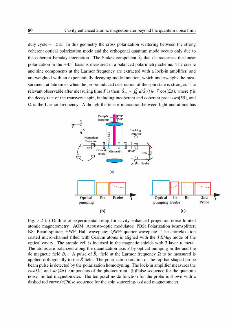
80 Cavity enhanced atomic magnetometer beyond the quantum noise limit
duty cycle ∼ 15%. In this geometry the cross polarization scattering between the strongcoherent optical polarization mode and the orthogonal quantum mode occurs only due tothe coherent Faraday interaction. The Stokes component Sy that characterizes the linearpolarization in the ±45o basis is measured in a balanced polarimetry scheme. The cosineand sine components at the Larmor frequency are extracted with a lock-in amplifier, andare weighted with an exponentially decaying mode function, which underweighs the mea-surement at late times when the probe-induced destruction of the spin state is stronger. Therelevant observable after measuring time T is then: Sy,c ∝
∫ T0 dtSy(t)e−γt cos(Ωt), where γ is
the decay rate of the transverse spin, including incoherent and coherent processes[55], andΩ is the Larmor frequency. Although the tensor interaction between light and atoms has
HomodyneDetection
HWP
HWP
QWP
Optical cavity
Microcell
RF
Coi
l
Pump&Repump
ProbeAOM
PBSPBS BS
Locking Detector
X
Y
Z
(a)
Optical pumping
Brf Probe Optical pumping
Brf 2ndProbe
1st Probe
t t
(b) (c)
Fig. 5.2 (a) Outline of experimental setup for cavity enhanced projection-noise limitedatomic magnetometry. AOM: Acousto-optic modulator; PBS: Polarization beamsplitter;BS: Beam splitter; HWP: Half waveplate; QWP: quarter waveplate. The antirelaxationcoated micro-channel filled with Cesium atoms is aligned with the T EM00 mode of theoptical cavity. The atomic cell is inclosed in the magnetic shields with 3-layer µ metal.The atoms are polarized along the quantization axis x by optical pumping in the and thedc magnetic field Bx . A pulse of Brf field at the Larmor frequency Ω to be measured isapplied orthogonally to the B field. The polarization rotation of the top-hat shaped probebeam pulse is detected by the polarization homodyning. The lock-in amplifier measures thecos(Ωt) and sin(Ωt) components of the photocurrent. (b)Pulse sequence for the quantumnoise limited magnetometer. The temporal mode function for the probe is shown with adashed red curve.(c)Pulse sequence for the spin squeezing-assisted magnetometer.

5.2 Quantum noise limited RF magnetometer 81
been used to enhance the magnetometer sensitivity[55], the magnetometer data presented inthis work were taken at large enough probe detuning (∆ = 1.6GHz blue detuned from theF = 4 7→ F ′ = 5 D2 transition) so that we can keep the vector interaction only, and neglectthe second rank tensor polarizability.
5.2.4 Results
Atomic density
As mentioned in the beginning of this chapter, one way to improve magnetometer sensitivityis to increase the density of alkali-metal atoms. The heating is realized by a twisted wirewith high resistance wounded around the aluminum cylinder where most of the magneticcoils are attached. By adding current on this wire a stable temperature can be establishedinside the cylinder. Figure 5.3 presents the spin response to a fixed RF excitation as afunction of the environment temperature. Since the atomic ensemble is prepared in thehighly oriented state (98% spin orientation) and the photon number is fixed during thismeasurement, the spin response is linearly proportional to the number of atoms as shown inEquation 5.1. In Figure 5.4, the experimental results for the RF magnetic field sensitivity
18 20 22 24 26 280.8
1
1.2
1.4
1.6
1.8
2
2.2
Temperature[ °C]
Nor
mal
ized
Res
pons
e
Steady state
Fig. 5.3 Normalized spin response to the fixed RF excitation as a function of the environmenttemperature.
as a function of the probe power are plotted when the duty cycle of the probe pulse is 100%and the backaction coupling constant C = 1. In the measurement the spin vector is kickedby applying a 8ms RF magnetic pulse at the Larmor frequency of 380kHz with the RMSamplitude of Br f = 243pT and the resulted non-zero mean value is then mapped onto thelight fieldSout
y . The geometric design and calibration of the magnetic system can be foundin Appedix 1 and the corresponding measurement details can be found in [34]. Due to

82 Cavity enhanced atomic magnetometer beyond the quantum noise limit
0 200 400 600 800
0.3
0.4
0.5
0.6
0.7
Cavity output probe power[nW]
Sens
itivi
ty [p
T/sq
rt(H
z)]
27°C
20°C
Fig. 5.4 Magnetic sensitivity versus cavity output probe power at 20C and 27C. Since theduty cycle of the probe pulse is 100%, the backaction coupling constant is C = 1.
increasing the atomic density by a factor of ∼ 2.2, the best sensitivity in the continuousprobing scheme is improved from 338.7fT/
√Hz to 235.0fT/
√Hz, a factor of 1.44, which
is in agreement with the theoretical prediction of Bsenr f ∝ 1/
√Na.
Optimal duration of the RF magnetic pulse
The duration of the RF magnetic pulse chosen above is an optimal value depending on themagnetometer bandwidth δA = 1/T2. Let us simply look at the physical idea inside. Whenthe initial spin state is prepared in the CSS state by optical pumping which corresponds tothe minimal transverse spin variances Var(Jy) = Var(Jz) = Jx/2, the projection noise limitedsensitivity to the magnetic field can be expressed as
Bsen = Bmin√
T
= [Ω/B√
FNA/2T1T2(e−T/T1 − e−T/T2)/[(T1 −T2)]]−1 ·
√T .
(5.7)
If assuming T1 ≫ T2, PN-limited magnetic sensitivity in two extreme situations of the dura-tion of rf pulse can be expressed as
Bsen
≈ [Ω/B
√FNA/2]−1 1√
TT ≪ T2
≈ [Ω/B√
FNA/2]−1√
TT2
T2 ≪ T ≪ T1(5.8)
In Figure 5.5, I plot the sensitivities calculated from these two extreme cases (blue curverepresents the case for T ≪ T2, and violet curve gives the sensitivity for T ≫ T2), andalso the theoretical prediction from Equation 5.7. Roughly speaking, when the duration ofRF-pulse T ≈ T2 one can achieve the best sensitivity. Figure 5.6 gives the experimental

5.2 Quantum noise limited RF magnetometer 83
0 1 2 3 4 50
0.5
1
1.5
2
2.5
3
3.5
4
rf dur [1/(T2)]
Nor
mal
ized
Sen
sitiv
ity
Fig. 5.5 Optimal duration of rf-pulse. Blue curve represents the case for T ≪ T2, and violetcurve gives the sensitivity for T ≫ T2. The theoretical prediction from Equation 5.7 ispresented as red curve.
demonstration with the optimal probe power of 200nW.
0 0.5 1 1.5 20.3
0.4
0.5
0.6
0.7
rf dur [1/T2]
sens
itivi
ty [p
T/sq
rt(H
z)]
Fig. 5.6 Magnetic sensitivity versus the duration of RF pulse. Since the duty cycle of theprobe pulse is 100%, the backaction coupling constant C = 1.
Quantum noise limited magnetometer
We now focus on the quantum noise limited RF magnetometer based on backaction evasionmeasurement. As described before by stroboscopically pulsing the probe beam at twice thefrequency of Larmor spin precession, the backaction evading measurement can be realized.In this measurement, by tuning the phase of cos(Ωt) component on the Lockin Amplifier,we can transfer the spin response signal into the cos(Ωt) component of the measured lightfield Sout
y . At the same time the phase between the synchronous intensity-modulated signal

84 Cavity enhanced atomic magnetometer beyond the quantum noise limit
and the RF-pulse signal should be optimized to reach the maximal response. Thus, thesignal to noise ratio can be simply calculated as
SNR =
∣∣Souty,c∣∣√
Var(Souty,c )
In Figure 5.7, the measured sensitivities as a function of probe power for two protocolsat 27C are plotted. As we expected, the best sensitivity is improved by a factor of 1.48,and also after some probe power the decoherence induced by spontaneous emission getsobvious which strong enough to change the trend of monotonically decreasing sensitivityand furthermore obstructs the realization of an ideal PN-limited magnetometer. However,the best sensitivity achieved here is 158±1.17fT/
√Hz.
0 200 400 600 8000.15
0.2
0.25
0.3
0.35
0.4
0.45
Cavity output probe power[nW]
Sens
itivi
ty [p
T/sq
rt(H
z)]
15% duty cycle100% duty cycle
Fig. 5.7 Magnetic field sensitivity versus cavity output probe power at 27C. The red circleshows the sensitivity when probe pulse is not modulated, while the blue circle presents thesensitivity when the probe beam is stroboscopically pulsed at twice the frequency of Larmorspin precession with 15% duty cycle. The measurement was performed at 380kHz with theoptimized RF pulse duration of 8ms.
5.3 Magnetic sensitivity beyond the quantum noise limitby spin squeezing
5.3.1 Protocol
Having demonstrated the back action evading magnetometer and projection noise limitedperformance, we have been able to make one step further and overcome this limit by sand-wiching the RF pulse between two back action evading measurements as shown in Figure

5.3 Magnetic sensitivity beyond the quantum noise limit by spin squeezing 85
5.2c. As demonstrated in the previous work[21, 22, 74], a sufficiently strong quantum non-demolition (QND) measurement can generate a spin squeezed state (SSS) of the measuredvariable. In the context of magnetometry SSS generated by the first optical pulse is followedby the magnetic field pulse to be measured. The cycle is completed by the second opticalpulse which measures the displacement of the SSS caused by the magnetic field. In[55] thisapproach was used for magnetometry with two atomic ensembles for which a light-matterinteraction without stroboscopic modulation generates a two mode squeezed state. Here,we use the stroboscopic QND measurement of Jz to generate a SSS state and to realize themagnetometer beyond the quantum noise limit. Let us denote the variances of the first andsecond probe pulses as Var(S1
y) and Var(S2y), respectively. The conditional variance of S2
y
expressed as Var(S2y |S1
y) = Var(S2y)−
Cov2(S1y ,S
2y)
Var(S1y)
, is reduced due to quantum correlation be-
tween the spin states probed by the two pulses. This noise reduction which leads to theimproved sensitivity is dependent on the covariance of S1
y and S2y , Cov2(S1
y , S2y).
5.3.2 Experimental results
In Figure 5.8, we plot the magnetic sensitivity as a function of radio-frequency bandwidth,where we see an improvement of 13% due to employing the conditional SSS and this im-provement vanishes when the RF-pulse duration reaches 3ms. The most pronounced im-provement occurs at a higher bandwidth (shorter RF-pulse duration) due to the decoherenceof the spin state between the two measurements.
0.2 0.4 0.6 0.8 1 1.2 1.4 1.6200
250
300
350
400
450
500
550
RF BW [kHz]
Sen
sitivity
[fT/s
qrt
(Hz)
]
No spin−squeezingSpin−squeezing assisted
Fig. 5.8 Sensitivity for stroboscopic modulation and entanglement-assisted scheme. Duringthe probe pulses, the average cavity output power is fixed at 100nW, with the interactiontimes of 1ms and 2ms,respectively.

86 Cavity enhanced atomic magnetometer beyond the quantum noise limit
5.4 Effect of optical cavity
As described in this thesis, a microcell coupled into an optical cavity is the key elementof the experimental setup whose optical depth is enhanced by a factor of 2F/π . Here Iwill explain the reason of introducing an optical resonator in detail. Let us denote thepower transmission coefficients of the input and output couplers, the round trip intracavitylosses, and atomic single pass absorption as T1,c, T2,c, lcav and d∆, respectively. The cavitypower transmission coefficient on resonance is 4T1,cT2,c/(T1,c+T2,c+ lcav+2d∆)
2. With theassumption of 2d∆ ≪ T1,c +T2,c + lcav, this coefficient can be expended as 4T1,cT2,c/(T1,c +
T2,c + lcav)2 · (1−2Fd∆/π), where F= 2π/(T1,c +T2,c + lcav) is the cavity finesse. Clearly,
the single pass atomic absorption d∆ is enhanced by a factor of 2F/π . From Kramers-Kronigrelations the phase shift, and therefore the polarization rotation angle, is enhanced by thesame factor. The input-output relations presented in Chapter 2 is modified by enhancingthe light-matter coherent interaction by 2F/π . If κ0 is the coupling constant in the absenceof cavity, then for the same number of detected photons in the pulse the cavity-enhancedcoupling constant is κcav =
2Fπ
κ0.
When back-action noise exists, SNR ∝ κ/√
1+κ2 +κ4/3 will always reach the upperbound when κ2 =
√3 if we do not consider the spontaneous emission due to d ≫ 1. In this
sense, introducing the optical cavity cannot give a significant improvement on the magneticfield sensitivity except the reduction of decoherent process. We have done this comparisonin the continuous magnetometer measurement using Microcell C7 with T2 ∼ 5ms whichgives the finesses of 10 when coupling into the optical cavity. (R1 = 99.97% and R2 = 80%).As shown in Figure 5.9, with the help of optical cavity, we only gained an improvement ofmagnetic sensitivity by 6%.
In the case of the back-action evasion, the optical cavity can improve the sensitivityfurther, since in this case SNR ∝ κ/
√1+κ2. In addition, with the presence of the optical
cavity, the conditional spin squeezing can also be improved where the realized squeezingis limited by the noise due to decoherence events. The probe-induced decoherence noise isproportional to the intracavity light-power experienced by the atomic ensemble Pin, whichis related to the power at the output of the cavity (Pout) through: Pout = Pin(
2T2c
−1), whereT2 is the output mirror coupler power transmission. For a standing wave cavity, maximumsqueezing is achieved for T1c ≪ T2c, so that the quantum light field generated inside thecavity from the interaction with the atoms has very small losses to the unobserved direction.Assuming only probe-induced decoherence and for T1c ≪ T2c ≪ 1, ξ 2 can be written in the

5.4 Effect of optical cavity 87
0 500 1000 1500 20001.95
2
2.05
2.1
2.15
2.2
2.25
2.3
2.35
Probe power (nW)
Sens
itivi
ty (p
T × H
z−1
/2 )
(a)
0 50 100 150 200 2501.8
1.9
2
2.1
2.2
2.3
2.4
2.5
Cavity output power (nW)
Sens
itivi
ty(p
T× H
z−1
/2 )
(b)
Fig. 5.9 Magnetic sensitivity of Continuous RF magnetometer without optical cavity (a) andwith optical cavity (b), respectively. Larmor frequency Ω:84.5kHz, and the spin orientationis above 90% by sending 59µW repump beam and 16µW pump beam.
formξ
2 =1
1+(2F/π)2κ20+η0(
2T2c
−1)
≈ 11+(2F/π)2κ2
0+η0
F(T2c + lcav)
πT2c
(5.9)
where η0 is the decoherence noise due to the light-probe in the absence of the cavity for thesame detected probe power.. For small but finite intracavity losses, optimizing with respectto the number of photons in the light pulse (κ0) and the output coupler transmission, thesqueezing is:
ξ2opt ≈ (2−
√h
(2F/π)d0)
√h
(2F/π)d0≈
√h
(F/2π)d0(5.10)
with the optimal T opt2 = lcav and κ2
0,opt =
√(d0/h)(2F/π)−1
(2F/π)2 . However, the intensity transmis-sion of the output coupler in the current setup is 20% which is a little bit higher than theintracavity loss 13%. Therefore, if we can match those two values in next step, we believethe spin squeezing can be improved.

88 Cavity enhanced atomic magnetometer beyond the quantum noise limit
5.5 Conclusion and outlook
In conclusion, we report a projection noise limited optical magnetometer at room tempera-ture with an RF magnetic-field sensitivity of 158± 1fT/
√Hz and 2D spatial resolution of
300µm. It utilizes a microfabricated Cs vapor cell with antirelaxation coating coupled intoan optical cavity to enhance the light-atoms interaction. Combining the stroboscopic back-action evading measurement with the cavity enhanced interaction, we improve the sensitiv-ity beyond the quantum noise limit by 13%. The room temperature quantum magnetometerdescribed here may find applications in many fields, such as biological and medical sensing.

Chapter 6
Deterministic quantum teleportationbetween distant atomic objects
6.1 Introduction
In this chapter I describe the "Deterministic quantum teleportation between distant atomicobjects" experiment. The results have been published in Nature Physics. As a key ingredi-ent in quantum networks and one of the building blocks for quantum computation, quantumteleportation, originally introduced for discrete variables[1] and later adapted for continuousvariables[75], denotes the transfer of a quantum mechanical state without the transmissionof a physical system carrying this state. The first experimentally realized teleportation pro-tocols employed light as the carrier of the quantum states[76, 77]. Also several protocols foratoms were realized, e.g. using two closely positioned ions [78] and later two ions in inde-pendent vacuum chambers separated by one meter[79]. Most protocols for distant atoms oratomic ensembles at the sending and receiving end are conditional in nature, such that eitherthe measurement outcome determines the success of the protocol or a heralded entanglementgeneration is employed. Whereas probabilistic teleportation, in which entanglement is dis-tributed by photon counting, is capable of reaching distances of many kilometres[80], thepower of continuous-variable teleportation is that it succeeds deterministically in every at-tempt, that it is capable of teleporting complex quantum states[81] and that it can be usedin universal quantum computation[82]. Here, we present an atomic teleportation experi-ment that works deterministically and on demand where a state transfer of the the spin statebetween two atomic ensemble of NA ≈ 1011 Cesium atoms at room-temperature is realized.

90 Deterministic quantum teleportation between distant atomic objects
6.2 Teleportation protocol
a†us
a†ls
b†F=4
F’=5,4,3
m=3 m=4
b c
pumpingmagnetic RF, cell 2magnetic RF, cell 1DC magnetic field pulsedrive-light t2-4ms 2ms
step I II III IV
H~( -a b a b+...)† † †us ls
atomsx ,pin in
lighty ,qin in
atomsx ( ,out x y ,q ),...p (x ,y ,q ),...
in in in
out in in inc,+ s,+
s,+ c,+
lighty (x ,p ,y ,q )...q (x ,p ,y ,q ),...
out in, in in in
out in, in in in
inte
ract
ion
10-15msd
B-field B-field
1. entanglement 2. joined measurement
light and atomic ensemble Bget entangled via interaction
joined measurement of light and ensembleAby interaction and measurement
3. feedback
-
measurement results are send to Bob+ local transformation via a RF pulse
B-RF
a
Fig. 6.1 The experimental layout. A strong driving pulse propagates first through ensem-ble B creating the modes xL = y′, pL = q′entangled with B and then through ensemble Awhose state is to be teleported. Joint measurements on the modes y′′ are performed usingpolarization homodyning. Teleportation is completed by classical communication of theseresults to B. See the text for further details. RF, radiofrequency. b, The level scheme andrelevant transitions. Classical drive field (thick lines) and quantum fields forming the modesy;q (wavy lines) are shown. d, The time line of the experiment. I, preparation of the inputstate; II, entanglement and joint measurement; III, feedback; IV, read-out of the teleportedstate. In the (c) the effect of the interaction with this linear Hamiltonian H is depicted. Wechoose to consider the atomic operators in the rotating frame, so that they are not mixed inthe interaction.

6.2 Teleportation protocol 91
A standard teleportation scheme involving the three parties Alice, Bob and Charlie con-sists of the following three steps, which allow Alice to teleport a quantum state providedby Charlie to Bob. (i) Alice and Bob establish an entangled link, which is shared betweenthe two remote parties. (ii) Alice performs a Bell measurement on her part of the entangledstate shared with Bob and an unknown quantum state prepared by Charlie. (iii) Alice uses aclassical channel to communicate the measurement outcome to Bob, who performs a localoperation on his quantum state conditioned on Alice’s result. In our experiment these twoobjects are an atomic ensemble at site B and a photonic wave packet generated by interac-tion of this ensemble with a driving light pulse (see Figure 6.1). The wave packet travels tosite A, the location of the atomic ensemble whose state is to be teleported. This step estab-lishes a quantum link between the two locations. Following the interaction of ensemble Aand the wave packet, a measurement is performed on the transmitted light. The results ofthis measurement are communicated through a classical channel to site B, where they arefed back through local operations on the second entangled object, that is, ensemble B, thuscompleting the process of teleportation.
6.2.1 Generation and distribution of the Einstein-Podolsky-Rosen en-tangled state
As discussed in[83], EPR entangled state is required to establish the quantum channel be-tween two stations involved in the quantum teleportation protocol which should satisfy ageneric condition in the continuous-variable regime for Gaussian states as mentioned interms of Var(X1 − X2)+Var(P1 + P2) < 2 where the canonical variables follow the canon-ical commutation relation [Xi,X j] = 0 and [Xi,Pj] = iδi j. In our scheme, an entanglinginteraction a†
usb† +H.C. is taking place, where one atomic excitation b† = (xB + pB)/
√2
is accompanied by the creation of a photon a†us in the upper sideband of the x-polarization
mode. This kind of light-atom entanglement generation is discussed in detail in Chapter 2,and the full Hamiltonian can be written as
Hint =ha2
∫ L
0dz[(ζ 2 +1)(aLb†
A + a†LbA)− (1−ζ
2)(a†Lb†
A + aLbA)]
∝ [(ζ 2 +1)HBS − (1−ζ2)HT MS]
where the normalized collective ground state spin operators in the rotating frame at Ω arexA,B = JA,B
y /√
Jx and pA,B = JA,Bz /
√Jx which follow the canonical commutation relation
[xA,B, pA,B] = i with variances var(x) = var(p) = 1/2 for the CSS, while the correspondingvariables for the upper sideband light mode are defined in Equation 2.51. From the Hamilto-

92 Deterministic quantum teleportation between distant atomic objects
nian above, it is found that the weight coefficients are related to the ratio between vector andtensor coupling strength as ζ 2 = 14a2
a1. In other words, the relative strengths of two different
interaction can be changed by detuning the laser frequency. The satisfaction of conditionVar(Xup
L − xoutB )+Var(Pup
L + poutB ) < 2 proves the establishment of entanglement between
an atomic ensemble at site B and the light field which is then sent to Alice at site A.
6.2.2 Bell measurement at Alice’s station
The spin information to be teleported of ensemble A is displaced with mean values ⟨xA⟩and ⟨pA⟩ by a weak radiofrequency magnetic field pulse of frequency corresponding tothe creation of a coherent superposition of electronic ground states mF = 3 and mF = 4.The following interaction between light field and atomic ensemble A at site A leads topartial mapping of its state onto light and is followed by the Bell measurements on thelight modes of the upper and lower sidebands performed using polarization homodyningwith the driving light acting as the local oscillator yielding Xc
L = 1√2(xup + xlow) and X s
L =1√2(plow− xup). The measurements of Xc
L and X sL serve as the joint measurement of ensemble
A and the light coming from site B. As mentioned before in order to compensate the atomicdecay, an exponential mode function is applied, and thus the read-out mode is xc/s,− ∝∫ T
0 dtx(t)e−γt cos/sin(Ωt) where T is the pulse duration and γ is the decay rate of the atomicstate. The completed input-output relations about xc/s,− including the tensor interaction canbe found in Equation 2.38 or [32].
6.2.3 Classical communication and feedback at Bob’s station
The teleportation protocol is completed by sending the measurement results xoutc/s,− through a
classical link to the site B with gain gx = gp = g where spin rotations in the y-z plane condi-tioned on these results are performed using phase- and amplitude controlled radiofrequencymagnetic field pulses at frequency Ω. The final canonical variable of atomic ensemble Bis[32] (
xteleB
pteleB
)= CB
(xin
B
pinB
)+CA
(xin
A
pinA
)+CA,N
(F in
xA
pinpA
)
+CB,N
(F in
xA
pinpA
)+Cx
(xin
s, fxxin
c, fx
)+Cp
(pin
c, fp
−pins, fp
),
(6.1)

6.3 Experimental realization 93
where the modes appearing in this equation are defined as
fN,B =√
2γextra[e−γ(T−t)+
√2γsγg
ζ√
1− e−2γT
∫ T
tdτe−γ(2τ−t)[1−2γs(τ − t)]],
fN,A =
√γsγextrag
ζ√
γ√
1− e−2γT(e−γt − e−2γT+γt),
fx =−ζ√
2γse−γ(T−t)+γsg
√γ√
1− e−2γT
2γ
γse−γt
− γsg√
γ√
1− e−2γT[e−γt(2− γs
γ)− e−2γT+γt(2− γs
γ−2γs(T − t))],
fp =
√2γs
ζe−γ(T−t)+
γsg
ζ 2√γ√
1− e−2γT(2− γs
γ)e−γt
− γsg
ζ 2√γ√
1− e−2γTe−2γT+γt [2− γs
γ−2γs(T − t)],
and the corresponding normalization factors read
NB/A =∫ T
0dt fN,B/A(t)
2, Nx/p =12
∫ T
0dt fN,x/p(t)
2,
while the coefficients appearing in the equation above are given by
CB = e−γT +
√γsg
ζ√
2γ[√
1− e−2γT (1− γs
γ)+2γsT
e−2γT√
1− e−2γT],
CA =
√γsg
ζ√
2γ
√1− e−2γT ,
CB/A,N =√
NB/A,Cx/y =√
Nx/y,
6.3 Experimental realization
6.3.1 Experimental setup
The layout and the time sequence for teleportation and verification are shown in Figure 6.1.A y-polarized, 3ms-long 5.6mW drive light pulse is sent through ensemble B which is bluedetuned from the D2 line F = 4 → F = 5 transition by ∆ = 850MHz. The interaction createsthe entanglement between the x-polarized forward scattered mode and the the collective spinB. The quantum light co-propagating with the drive light is then directed through ensembleA where the dispersive interaction leads to partial mapping the spin state of atomic ensembleA onto the light field, and then a measurement of one of the quadrature operators ∼ Sy in

94 Deterministic quantum teleportation between distant atomic objects
Cesium cell
Rf-coilsMagnetic shielding
Fig. 6.2 Two glass cells filled with Cesium are shown on the left. The square glass cellconsisting NA ≈ 1011 ∼ 1012 atoms is used in this quantum teleportation experiment whichis situated in a magnetic shield shown on the right. The bias magnetic field of 0.9G ispointing out of the picture plane here and is created by four coil pairs. The RF coil areoriented such that the RF field lies orthogonal to the bias field and macroscopic spin. Twoapertures along the transversal direction allow the light beam to pass the cell. The pumpbeams are aligned in direction of the main axis and also a small and weak probe light beamto monitor the atomic density by measuring the Faraday angle directly.
the x-polarization mode behind the ensemble constitutes the Bell measurement where asmentioned in the protocol section the driving light acts as the local oscillator to perform thepolarization homodyning detection. The photocurrent is analyzed with a lock-in amplifierat Ω and further computer processed to obtain measurements of the temporal modes ofinterest to compensate the atomic decay where an exponential mode function is applied, andthus the read-out mode is xc/s,− ∝
∫ T0 dtx(t)e−γt cos/sin(Ωt). The teleportation protocol is
completed by sending the measurement results xoutc/s,− through a classical link to the site B
with gain gx = gp = g where spin rotations in the y-z plane conditioned on these resultsare performed using phase- and amplitude controlled radiofrequency magnetic field pulsesat frequency Ω. The deterministic character of homodyne process ensures success of theteleportation in every attempt. It should be noticed that experimentally for the read-out ofeach individual ensemble the other ensemble is detuned from the atom-light interaction bybriefly detuning the B field in the respective cell.
6.3.2 Experimental results
The reconstruction of the collective spin state as described before relies on the input-outputrelation of light variables, and for the off-resonant light-atom interaction this linear trans-

6.3 Experimental realization 95
formation is given as
xoutc/s,− = κ · pA/xA + cx · xin
c/s, fx + cp · pinc/s, fp
+ cN · Fp/x,
Here, the first term is a contribution of the atomic spin variable due to Faraday rotation oflight polarization, the second term is proportional to the input value of the light quadraturexL of the temporal mode fx and the third term is the contribution of the other quadratureof input light pL of temporal mode fp resulting from back action of light on atoms (seeSupplementary Information). All input light modes are always in a coherent or vacuum statewith Var(xin
c/s, fx) = Var(pin
c/s, fp) = 1/2. The last term describes additional noise arising from
atomic decoherence with Var(Fp/x) = m/2 with m = 1.3 calculated from the atomic spinrelaxation[29]. In our experiment since A y-polarized, 2ms-long 5.6mW light pulse bluedetuned from the D2 line F = 4 → F = 5 transition by ∆ = 850MHz drives the interaction,ζ 2 = 1/6.3 is calculated from Clebsh-Gordon coefficients and experimentally verified whilethe relaxation rates are measured with the results of γ = 99.3± 0.2s−1 and γextra = 26.3±0.2s−1. The coupling strength is measured as κ = 0.87 by using the mean value transfer[35].According to these measured parameters the coefficients shown in equation above can befound with the values of cx = 0.93, cp = 0.50 and cN = 0.17. Additionally, For the atomic-state reconstruction the detection efficiencies including optical losses ηB = 0.8± 0.03 andηA = 0.89±0.03 for ensembles B/A are taken into account. Using equation above the meanvalues of the input states of ensemble A are found from measurements of light variables as⟨xA⟩=
⟨xA
c,−⟩/κ and ⟨pA⟩=
⟨xA
s,−⟩/κ with the variance of Var(xA) = (Var(xc,−)− c2
x/2−c2
p/2− c2Nm/2)/κ2 and Var(pA) = (Var(xs,−)− c2
x/2− c2p/2− c2
Nm/2)/κ2. It is found thatthe initial spin state with the variance of Var(xA) = Var(pA) = (1.03±0.03) ·1/2 is close tothe coherent spin state.
6.3.3 Fidelity
To verify whether or not a successful quantum teleportation event is performed, the fidelityof state transfer is compared to the classical benchmark fidelity which has a rigorous formof (1+ n)/(1+ 2n) [84] where n =
⟨b†b⟩
is the mean number of spin excitations for thedisplacement of Gaussian distribution. The performance of the protocol is assessed usingthe average fidelity with respect to a Gaussian distribution of coherent input states as figureof merit. The fidelity is given by the overlap of the final atomic state in ensemble B
∣∣ΨteleB⟩,
which is described by xteleB and ptele
B and the optimal final state which is defined by the initialstate in ensemble A xin
A and pinA . For a given coherent input state with mean values ⟨xA⟩ and

96 Deterministic quantum teleportation between distant atomic objects
⟨pA⟩, the single-shot fidelity is given by
F(⟨xA⟩ ,⟨pA⟩) = 2e−
−|⟨xA⟩−⟨xteleB ⟩|2
1+2Var(xteleB )
− |⟨pA⟩−⟨pteleB ⟩|2
1+2Var(pteleB )√
(1+2Var(xteleB ))(1+2Var(ptele
B ))(6.2)
such that the average fidelity F(n) with respect to a Gaussian distribution with width n
F(n) =1
2π n
∫ ∫∞
−∞
d ⟨xA⟩d ⟨pA⟩F(⟨xA⟩ ,⟨pA⟩)e−⟨xA⟩2
+⟨pA⟩2
2n
=
√√√√ 2
1+2Var(xteleB )+2n(1−
∣∣∣ ⟨xB⟩⟨xA⟩
∣∣∣)2·√√√√ 2
1+2Var(pteleB )+2n(1−
∣∣∣ ⟨pB⟩⟨pA⟩
∣∣∣)2.
(6.3)
n=0,5, 25
Fig. 6.3 The mean value of different input states.
Experimentally, we perform the teleportation using various sets of CSSs of ensembleA with varying
⟨Jy,z⟩, corresponding to displaced vacuum (coherent states) as input states
shown in Figure 6.3 (the vacuum, the CSS with displacements of 5 in vacuum units andphases 0,π/4,π/2, and the CSS with displacements of 25 in vacuum units and phases0,π/4,π/2). For every input state, 10,000 ∼ 20,000 teleportations have been performedwith one full cycle of the protocol lasting 20ms. Figure 6.4 (a) shows the variance of theteleported states as a function of gain g. The quadratic dependence of the variances on g pre-dicted by the model fits the experimental data very well. For a certain range of g the atomicvariances are reduced owing to the entanglement of the transmitted light with ensemble B.Figure 6.4 (b) presents the experimental fidelity, which is above the classical benchmarkfor n 6 7. The blue dots represents the scheme that the feedback is done by preforming adisplacement with a radio-frequency pulse applied to ensemble B, followed by a readingpulse to verity the atomic states, while the red dots give the results in the scheme that theverification read-out is done firstly, followed by the displacement operation applied to the

6.3 Experimental realization 97
0 0.5 11
2
3
4
5
6
gain
AN
[P
N u
nits
]
2 4 6
0.55
0.6
0.65
0.7
nF
nn
a b
Fig. 6.4 (a) The variances of the teleported state Var(xtele, ptele) as a function of gain.(b)Teleportation fidelity as a function of the mean photon number of the set of states. Tele-portation with radio-frequency feedback (blue dots), feedforward teleportation (red dots),and classical benchmark (black dashed line). Error bars present one standard deviation.
result of measurement numerically. The worse performance of radio-frequency feedbackscheme is due to introducing of additional technical errors.
10
5
0
5
10
10
5
0
5
10
10
5
0
5
10
10
5
0
5
10
1sty /(κ/√2)c
2ndy /(κ/√2)c
1sty /(κ/√2)s
2ndy /(κ/√2)s
input outputscan
<x >A
<p >A
<x >tele
<p >tele
1sty /(κ/√2)c
1sty /(κ/√2)s
2ndy /(κ/√2)c
2ndy /(κ/√2)s
timeevolution
Fig. 6.5 Teleportation with a dynamically varied input state. The input displacements of xA ∝
Bsr f , pA ∝ Bc
r f are varied in time as shown in the left column (Br f ≈ 1pT). The center/rightcolumn presents the readout of the input/teleported dynamics of the atomic spin A/B. Theupper/center row is the x/p variable and the lower row is a two-dimensional plot x/p. Everygray point is a teleportation run with the points taken at the rate of ∼ 50Hz.

98 Deterministic quantum teleportation between distant atomic objects
Stroboscopic teleportation of a sequence of spin states from A to B is shown in Figure6.5 where the repeated teleportation cycles are performed while varying the amplitude andphase of the input state. The left column shows the time-varying radiofrequency field in thepicoTesla range that is applied to prepare a new spin state A in each individual teleportationrun, after initializing both ensembles to vacuum between the runs. The central columnshows the read-out of the input-state evolution of ensemble A and the right column showsthe read-out of the teleported-state evolution. The points represent results for individualteleportation runs.
6.4 Conclusion and outlook
We demonstrate a missing element of the quantum teleportation landscape, the determin-istic continuous variable teleportation between distant material objects - room temperatureatomic spin ensembles. Entanglement required for teleportation is distributed by light prop-agating from one ensemble to the other. Quantum states encoded in the collective spin stateof one ensemble are teleported onto another ensemble spin using this entanglement and ho-modyne measurements on light. By implementing process tomography, we demonstrate thatthe experimental fidelity of the quantum teleportation is higher than that achievable by anyclassical process. Furthermore, we demonstrate the benefits of deterministic teleportationby teleporting a dynamically changing sequence of spin states from one distant object ontoanother.
The fidelity of the teleportation can be further improved by using time varying drivingpulses and increasing the optical depth of the atomic ensemble, as shown in[85]. Non-classical states can be efficiently teleported using continuous variable teleportation[81], andcontinuous variable teleportation of an atomic qubit encoded in a collective spin by a pho-ton scattering can be performed using the present approach. The stroboscopic teleportationof the spin dynamics can be also extended towards a true continuous in time teleportationpaving the way to teleportation of quantum dynamics and simulations of the interactionbetween two distant objects which do not interact directly. From the quantum sensing per-spective teleportation of spin dynamics would allow to perform measurements at the loca-tion spatially separated from the environment where the actual dynamics takes place.
Chapter 7
Conclusions and outlook
7.1 Conclusions
The micro-fabricated room temperature Cs vapor cell provides the opportunity to realizethe scalable quantum metrology and quantum information devices that can be readily inte-grated in larger quantum networks. For the cubic vapor cells with the size of 2.2cm sincethe density of atoms can not be increased much by heating due to the properties of the paraf-fin coating, and a higher optical power leaves us with technical difficulties in the detectionas well as problems with growing classical noise, there are limitations on the experimen-tally achievable coupling strengths. Also its limited bandwidth, due to the required timesfor atoms to pass through the laser beam impedes us to run some quantum protocols likegeneration of single-photon on demand.
By utilizing the microcells coupled into an optical resonator these problems can be over-come. Because of small beam area, the required number of photon is also reduced whichmeans that the weak light beam can satisfy the condition of atom-light interaction. Cavityenhanced optical depth by a factor of 2F/π can compensate the reduction resulted from thedecrease of cell size. Additionally, a 300×300µm2 cross section of our microcell sets theatomic transit time about 1 ∼ 2µsec, which can match the bandwidth of single excitation byusing a filter cavity following atom-light interaction system[53]. In this thesis, the atomicensemble of 107 ∼ 108 atoms is contained in a glass cell microchannel, 300× 300µm2 incross section and 1cm in length. A hole 10 ∼ 20µm in diameter is laser-drilled at the topsurface of the chip to create an entrance through which the channel is filled with Cs vapor.Windows with anti-reflection coating are attached at both ends of the microchannel to reducethe transmission losses. Currently, the intensity loss per window is about 3 ∼ 4%, limitedby the deterioration of the anti-reflection coating quality in the glass blowing phase. Analkene coating deposited on the inner cell surface can stand more than 104 collisions with

100 Conclusions and outlook
the Cs atoms before decoherence occurs, resulting in longitudinal spin lifetime T1 = 17msand transverse spin lifetime T2 = 10ms in the absence of light fields.
The microcell is placed inside a standing wave optical cavity consisting of a high-reflection input coupler and the output coupler with transmission of 80%. 6.5% single-passloss in the cell windows partially results in a finesse F ≈ 17. As discussed in Chapter 4the optimal squeezing can be achieved with an impedance matched cavity where the out-put coupler transmission T2 ≈ lcav, where lcav is the round-trip intensity loss. Thus, ourexperimental setting is close to this condition.
Based on this system we have experimentally developed the quantum backaction evad-ing measurement of one quadrature of collective spin components by stroboscopically mod-ulating the intensity of probe beam at twice Larmor frequency. Furthermore, a spin-squeezedstate conditioned on the light-polarization measurement with 2.2± 0.3dB noise reductionbelow the spin projection noise limit for the measured quadrature has been demonstratedwhich is be useful for quantum metrology and sensing, as well as for generation of entan-glement between disparate oscillators.
As an application of stroboscopic back-action-evading measurement, we demonstrateda quantum noise limited optical magnetometer at room temperature with an rf magnetic-field sensitivity of 158± 1fT/
√Hz and 2D spatial resolution of 300µm. Furthermore, by
sandwiching the rf pulse between two backaction evading measurements, an magnetometerwith 13% spin-squeezing below the projection noise limit was realized, where conditionalspin squeezed state generated by the first optical pulse, and then the second optical pulsemeasures the displacement of the SSS caused by magnetic field.
Deterministic quantum teleportation of the collective spin state from one atomic ensem-ble to another was reported in Chapter 6 where the cubic vapor cells with the size of 2.2cmwere employed. Then the stroboscopic teleportation of spin dynamics was demonstratedwith the fidelity higher than the classical benchmark. This can be extended to teleportationof quantum dynamics and simulations of the interaction between two distant objects thathave never interacted directly.
7.2 Outlook
High quality Microcells
As described in this thesis, atomic density, spin life time and intensity transmission arethree key parameters of the room-temperature vapor cell. We have achieved the reasonablevalues at the present stage. However, if for microcells inside optical resonators we really

7.2 Outlook 101
need to improve the fabrication to increase the intensity transmission and thus reduce theinformation loss of the system. In Chapter 5, the effect of optical cavity has been discussedwhere we derive the optimal variance spin squeezing as Var(XA) ∝
1√F
with the condition of
T opt2 = lcav and the round trip intra-cavity loss lcav is mainly determined by the optical loss
propagating trough the microcell. Additionally, for atoms inside an optical cavity, both theresonant single pass optical depth of the atomic ensemble d and the light-atoms coherentcoupling strength κ are enhanced by a factor of 2F/π . Although the good anti-reflectioncoated windows are employed, the current single-pass intensity loss of the microcell is about6.5% coming from the deterioration of the anti-reflection coating quality in the glass blow-ing phase, therefore, we are employing the CO2 laser bonding procedure to attach windowsat the edges of the cell, and attach a round tube to the cell’s top surface where the micro-holeis drilled.
Quantum sensor in the biological application
Our compact and simple optical magnetometer with high spatial resolution and sensitivity isa candidate to be used as a non-invasive biomagnetic sensor because it is room temperaturewhere life lives. At present we are in the early stages of a collaboration with the biologygroup and Membrane Biophysics group in the University of Copenhagen to study the nervesignals from frogs and lobsters. In Figure 7.1 we show an simulation experiment that sim-ulates a neuron pulse by sending a RF-pulse into the RF coil of one sinusoidal cycle withperiod of 0.3ms as shown on the right of top into the RF coil.The left top of Figure 7.1shows the spin response signal.
High efficiency single photon generator for DLCZ protocol
To achieve long-distance, high-fidelity, qubit teleportation, an architectures using neutralatoms was proposed by Duan, Lukin, Cirac and Zoller (termed DLCZ hereafter)[5]. InDLCZ scheme, entanglement distribution is accomplished by weak coherent driving of aRaman transition in an atomic ensemble followed by path-erasing photodetection. Althoughthe motion of the atoms destroys atomic superposition states in the thermal vapor cell, mo-tional averaging discussed in Chapter 2 can be used to realize room temperature quantummemories and coherent single photon sources where atoms move in and out of the beamseveral times during the interaction while maintaining the spin coherence for much longertimes. In [53], it is shown how both read and write efficiencies above 90% can be achievedfor a real experimental system based on Cs-atoms inside a microcell similar to the onedescribed in this thesis. Since the microcells have the potential to be integrated in semicon-

102 Conclusions and outlook
1
Fig. 7.1 Simulated biomagnetic experiment.
ductor chips, the fiber-coupled, integrated quantum repeater could be demonstrated in thefuture.
Nano-mechanical membrane-atomic ensemble interface
Since the existence of challenges for the optomechanical system to prepare, manipulate andmeasure quantum states with high precision, a quantum interface between atomic ensemblesand optomechanical systems has been proposed in [86], where light plays the role of aquantum bus. Furthermore, the establishment of quantum entanglement between an atomicspin oscillator with a negative mass and a mechanical oscillator coupled to light via radiationpressure can enable the trajectory of the mechanical oscillator to be measured with theprecision beyond the standard quantum limit. Soon, we will perform the first efforts tocouple the atomic ensemble in the microcell to a optomechanical system (membrane-in-middle type) which is sitting in the separate room at QUANTOP, and hope to see EPRentanglement between the atoms and the mechanical oscillator as the next step.

7.2 Outlook 103
Multipartite entangled states
Multipartite entangled states play a crucial role in quantum information processing. Re-cently, one special type of multipartite entangled states called graph state, has been proposed[87,88] and gradually became a key component of quantum information systems because it al-lows large scale quantum information tasks to be implemented orderly according to thespecific program. Cluster states as a well-known member of this family provide the uni-versal source for one-way quantum computation model where the system is firstly ini-tialized in a cluster state, independently of the quantum algorithm which is to be imple-mented and determined by different temporal and spatial sequences of series of the projec-tive measurements[89]. Correspondingly, one-way quantum computation based on clusterstates have been demonstrated experimentally both in DV[8] CV regime[7]. Additionally,graph states of optical field have been theoretically described in general[87, 88, 90], andgenerated in different structures experimentally[91, 92]. Since entanglement-assisted net-works communication with higher channel capacity than classical limit can be realized byapplying multipartite entangled states, graph states can also be used to set controlled quan-tum communication networks[93]. Due to specific quantum correlation of graph states, thechannel capacities between two users can be controlled and the signal-to-noise ratios cansurpass the shot noise limit of the classical optical communication. We can generate thiskind of hybrid multipartite graph state based on off-resonant Faraday interaction betweenlight and atoms[11, 94].


Appendix A
Details of the magnetic coil system
DC magnetic field
DC bias coil
The wire-coil system which creates the static field sits on an aluminum cylinder, which islocated insider 3-layers of µ-metal magnetic shields, thus providing an environment isolatedfrom external stray magnetic fields. The static bias magnetic field in the x-direction(quantizationdirection) is generated by sending a current through eight equally spaced coils with differ-ent numbers of windings similar to a solenoid. Although there exists the inhomogeneity inx-direction, due to 300µm dimension of the vapor cells this inhomogeneity has an insignif-icant effect on the measurements. However, the inhomogeneity in the propagation direction(z-direction) is important for the measurements. For large applied magnetic fields, this in-homogeneity, the coherence of spins leading to shorter spin life time. The Bx magnetic fielddistribution along z-direction is plotted in Figure A.1.
DC compensation coil in the probe propagation direction
The quadratic correction in the z-direction is accomplished via a double-saddle coil arrange-ment consisting of eight circular arcs[95], wound on the cylinder beneath the plastic rings.This geometry was initially designed to be used as a linear gradient coil with the currentdirection shown in the pink arrows; however, if changing the current direction as shownin the black arrows, this double-saddle structure can be used as a quadratic coil. In FigureA.3, the magnetic field distribution along z-direction is plotted. Currently, both 5-turn lineargradient and quadratic coils are located on the aluminum cylinder.

106 Details of the magnetic coil system
Position [mm]
Mag
netic
fiel
d[G
]
Fig. A.1 DC magnetic field distribution along z-direction with current I = 200mA and R =22.35Ohm.
Fig. A.2 Double-saddle compensation coil schematic drawing. The pink arrows show thecurrent direction for the linear gradient coil, and the black arrows show the current directionfor the quadratic coil.

107
Position [mm]
Mag
netic
fiel
d [G
]
Fig. A.3 Magnetic field distribution of the Bx component in z-direction generated by double-saddle compensation coil with current I = 200mA.
Weak bias magnetic field in the transverse directions
As discussed in the main text, the propagation direction of the probe beam should be per-pendicular to the direction of the DC bias magnetic field, which is parallel to the opticalpumping direction. Since the probe light is circulating in an optical cavity, it is difficultto satisfy this geometry by aligning the cavity field, and aligning the magnetic field insidethe shield by hand is not precisely. Therefore,of the Bx component in the y and z-directionare utilized as shown in Figure A.4 to create the homogeneous magnetic field in y and z-direction. In Figure A.4 the black and red symbols represent the current direction in thecopper wires for By and Bz magnetic field creation respectively. The θ angle of the co-sine windings can be calculated according to[96], and here we use 10.6, 30 and 56.5 togenerated the homogeneous weak bias magnetic field in a range larger than 2cm.
Calibration of the RF coil
In order to calibrated the RF coil, a pick-up coil with 30 turns copper wire is employedas shown in FigureA.5. The oscillating magnetic field creates a flux through the pick-upcoil which generates an electromotive force When applying a sinusoidal magnetic field offrequency omega and amplitute Br f . The current through the pick-up coil can be found frommeasuring the voltage amplitude Uω across the measurement resistor Rm [34].

108 Details of the magnetic coil system
By
Bz
Fig. A.4 Cosineθ coil in y(red symbols) and z(black symbols)-direction schematic drawing.The black and red symbols represent the current direction in the copper wires for By and Bzmagnetic field creation.
Fig. A.5 Photo of pick-up coil.

109
∣∣Br f∣∣= |1+Zcoil/Rm| |Uω |
NωAcoilω, (A.1)
The pick-up coil has the following parameters: number of windings Nω = 30, area of thecoil Acoil = πr2 = π(3.75mm)2, and the impedance Zcoil ≈ iω ·L at frequency ω with theinductance of L= 55µH, since the resistance of the coil R= 3Ω is much smaller than ω ·L atthe frequency we usually operate (380kHz). We use lock-in amplifier to read of the responsegenerated in the pick-up coil. Since the voltage is read out over the resistance Rm = 50Ω.The measured amplitude of the voltage is Uω =
√2Urms where Urms is the rms voltage.
0 500 1000 1500 20000
0.5
1
1.5
2
2.5
3
3.5x 10
−8
RF frequency [kHz]
BRF
RMS[
T]
(a)
0 0.5 1 1.5 2−0.5
0
0.5
1
1.5
2
2.5
3
3.5x 10
−8
Aplied Voltage [Vpp
]
Brfpp
[T]
y = 1.7e−008[T/V]*x[V] − 9.5e−011[T]
(b)
Fig. A.6 (a)The generated magnetic field Brmsr f for different frequencies. For all the fre-
quency range the same voltage was applied in the RF coil. Two different colors representthe calibration from Bing and Giorgos,respectively. (b) The measured Bpp
r f for differentapplied voltage at 322kHz with external resistor R = 20Ω. "pp" means peak-to-peak value.


Appendix B
Details of the microcell fabrication
1st-generation chip fabrication
These cell-chips with dimensions in the micrometer range were designed and fabricated byboth QUANTOP at Niels Bohr Institute and Danchip at DTU. As is shown in Figure 3.5, thefinished chip consists of 4 layers (for 5 layer-samples there is an additional glass layer onthe top of the whole structure). The cell is the narrow channel (200µm×200µm×10mm)in the middle glass and suitable holes in the middle silicon and bottom glass for Cs accesswere created.. There is no special process for the top silicon layer.
In the middle glass layer, a groove with a 200µm×200µm cross section was developedby Micro saw. Before the final decision of the cutting method, we have compared theperformance of Micro saw cutting followed by Chemical roughness reduction (treatmentwith HF:HCl mixture) with Micro saw cutting only. It was found that employing onlythe Micro saw cutting we can get the walls with roughness of 40nm as characterized by anoptical profiler. In order to etch a small funnel on the second silicon layer, Photo-lithographyand Etching were utilized successively to transfer the structures from mask to silicon wafer.Firstly, Nitride was deposited by low pressure chemical deposition (LPCVD) on the siliconwafer to develop a thin Nitride membrane that protects other part of the wafer to be etchedin the KOH etching. And then, we did the wafer exposure under 7W of ultraviolet laserlight for 5.6s which is followed by 60-second of development. We then make sure that thereis no resist visible by inspecting with optical microscope; otherwise Plasma Asher shouldbe used to clean it. Following exposure, the Nitride membrane covering the hole should beremoved to make sure the etching on the silicon can be conducted successfully which can bedone by using Reactive-ion etching (RIE) equipment. In addition the residual resist materialshould be striped by immersing the wafer into Acetone solution for several minutes. Afterthis preparation work, we can do the real silicon etching by utilizing KOH etching which

112 Details of the microcell fabrication
belongs to the family of anisotropic Si-etchants based on aqueous alkaline solutions. Duringthe etching process, we should check if the etch rate is appropriate. As mentioned above,the Nitride membrane can protect other part of the wafer from etching in the KOH solution,so this membrane covers the whole wafer except for the hole-structure and should be stripedby RIE. Until now, the funnel is produced on the silicon wafer and three different hole sizesare obtained (19µm, 29µm, and 54µm).
A large hole is required on the bottom layer glass which is the entrance for the evacu-ating, coating, and filling of the cell. To avoid the damage on the glass wafer, the wholeproduction of the large hole consists of two steps: laser marking and sand blowing. At thefirst stage, the laser burns the blue tape which sticks onto the wafer to protect it, and a littlebit of the glass surface. Then, the Aluminum Oxide 110µm in diameter spheres at highpressure are used to do the abrasive action. Finally, we obtain the 3mm hole on this glasswafer.
With those separated wafers as the components of final chip, we can combine themtogether by implementing the bonding process with the equipment of EVG NanoimprintLithography (NIL). The first bonding is to combine the glass grove wafer with the siliconfunnel wafer where a precise alignment is required. Here, anodic bonding is utilized, whichmeans we should place the Si wafer closest to the chuck and the Pyrex wafer closest to theelectrode. Secondly, we bond the two other wafers, that is the hole wafer and the untouchedsilicon wafer, resulting in a two-layer wafer. We complete a the chip production with cuttinginto small pieces of chips and polishing these chips.
Current generation chip fabrication
The bare chips with the channel are ordered from VitroCom and the bare windows are coatedwith anti-reflection coating in Denmark. The microholes were drilled by using a 50W,1064nm picosecond-pulsed Nd:YAG laser (neodymium-doped yttrium aluminium garnet) atthe Danchip facility.In order to encapsulate the microcell, anti-reflection coated windows arefused to the glass cylinder with the chip inside (with glass spacers placed around the chip)and also a glass stem with an opening is fused to the cylinder. The whole glass structureis annealed at above 550 to remove stresses that could lead to the optical birefringence asdiscussed before. Vacuum-tight test should then be done on the whole glass structure. Weare running the laser bonding procedure with CO2 laser now to replace the glass blowingand fusion phase.
The anti-relaxation coating procedure begins with the cleaning of micro-channel witha solution of hydrochloric acid, then rinsing with distilled water followed by the vacuum-

113
pumping. Heated coating material and Cesium are injected into the channel through themicro-hole, subsequently. To increase the atomic density and redistribute the coating ma-terial evenly, the microcell is cured for 3-4 hours at 60C and allowed to cool down slowlybefore being removed from the oven. At this time, the microcell fabrication is finally fin-ished. The glass blowing and coating procedures are operated by Mikhail Balabas (of the S.I. Vavilov State Optical Institute, St. Petersburg, Russia).


Appendix C
Phase-Locking and Frequency-Lockingsystem
PDH frequency stabilization
HWP Optical cavity
Locking Detector
HWPEOM
Isolator
~Local RF signal
MixerLow-pass
Filter PI
PZT
Laser
MonitorDetector
3 2 1 0 1 2 31.0
0.5
0.0
0.5
1.0
Frequency
Err
orsi
gnal
0.30.2 0.1 0.0 0.1 0.2 0.31.00.5
0.00.51.0
Frequency
Err
orsi
gnal
(a)
(b) (c)
Fig. C.1 (a)The basic layout for locking a cavity to a laser. (b)The PDH error signal,ε/2
√PsPc vs ν/ν f ree , when the modulation frequency is low. (c) The PDH error signal,
ε/2√
PsPc vs ν/ν f ree , when the modulation frequency is high.
The original scheme of PDH locking system is shown in Figure C.1. The Laser beamis frequency modulated by a Electro-optic modulator (EOM), driven by a local oscillator atfrequency Ωm and then injected in the optical cavity. The reflected beam from an optical

116 Phase-Locking and Frequency-Locking system
isolator is sent into a broadband photodetector. The output electronic signal is mixed withthe local oscillator’s signal via a mixer where the phase of this local oscillator can be tunedby internal or external delay line. Since the mixer is a device whose output is the product ofits inputs, this output will contain signals at both dc (or very low frequency) and twice themodulation frequency. The low frequency signal carrying the information of the derivativeof the reflected intensity can be picked up by a low-pass filter, and then goes through aproportional-integral controller (PI) and into the piezoelectric transducer (PZT), locking thecavity to the laser. Using the knowledge in Chapter 3, we can derive the reflection coefficientF(ν) as
F(ν) = Ere f /Ein =T1√
R1 −√
R1(1−g(ν))1−g(ν)
,
g(ν) = gme−iδφ =√
R1 ·R2(1− lcav)Exp[−i2π(νL −νcav)]
(C.1)
As given in[65], if the modulation frequency is very low with respect to the bandwidth ofcavity, the error signal after the low-pass filter can be written as
ε ≈ 2√
PsPcd |F(ν)|2
dνΩm, (C.2)
where Pc = J20(β )P0 and Ps = J2
1(β )P0 are the power in the carrier and in the first sidebandrespectively expressed in terms of the Bessel functions with modulation depth β and inputpower P0. Otherwise, if modulation frequency is high with respect to the bandwidth ofcavity, the error signal after the low-pass filter can be written as
ε ≈−2√
PsPcIm[F(ν)F∗(ν +Ωm)−F∗(ν)F(ν −Ωm)] (C.3)
The profiles of both case of high and low modulation frequency are plotted in Figure C.1(b) and (c), respectively.
Cavity phase locking by PDH-like locking
Since in our experimental, the cavity bandwidth is about 40MHz, and typically if one wantsto use the frequency modulation scheme the modulation frequency is several times the cavitybandwidth. It is hard to give such a high modulation frequency. Therefore, instead offrequency modulation on the light beam we send a 10kHz modulated voltage on the PZTattaching to the output mirror. And also we use a lock-in amplifier to replace the separatedelectronic components including local oscillator generator, mixer, low-pass filter and delayline. The observed error signal is similar to Figure C.1 (b). Additionally, PI controller based

117
on the Labview program is utilized to lock the cavity on resonance in the pulse schemewhere the locking point is in the memory.


Bibliography
[1] C. H. Bennett,G. Brassard,C. Crépeau, R. Jozsa, A. Peres, and W. K. Wootters, Tele-porting an unknown quantum state via dual classical and Einstein-Podolsky-Rosenchannels,Phys. Rev. Lett. 70, 1895 (1993).
[2] Charles H. Bennett and Stephen J. Wiesner, Communication via one- and two-particleoperators on Einstein-Podolsky-Rosen states,Phys. Rev. Lett. 69, 2881 (1992).
[3] Klaus Mattle, Harald Weinfurter, Paul G. Kwiat, and Anton Zeilinger, Dense Codingin Experimental Quantum Communication, Phys. Rev. Lett. 76, 4656 (1996).
[4] Xiaoying Li, Qing Pan, Jietai Jing, Jing Zhang, Changde Xie, and Kunchi Peng,Quantum Dense Coding Exploiting a Bright Einstein-Podolsky-Rosen Beam, Phys.Rev. Lett. 88, 047904 (2002).
[5] L.-M. Duan, M. D. Lukin, J. I. Cirac, and P. Zoller, Long-distance quantum commu-nication with atomic ensembles and linear optics, Nature 414, 413 (2001).
[6] C. Monroe, D. M. Meekhof, B. E. King, W. M. Itano, and D. J. Wineland, Demon-stration of a Fundamental Quantum Logic Gate, Phys. Rev. Lett. 75, 4714 (1995).
[7] Ryuji Ukai, Shota Yokoyama, Jun-ichi Yoshikawa, Peter van Loock, and Akira Furu-sawa, Demonstration of a Controlled-Phase Gate for Continuous-Variable One-WayQuantum Computation, Phys. Rev. Lett. 107, 250501 (2011).
[8] P. Walther, K. J. Resch, T. Rudolph, E. Schenck, H. Weinfurter, V. Vedral, M. As-pelmeyer, and A. Zeilinger, Experimental one-way quantum computing, Nature 434,169 (2005).
[9] P. W. Shor, Algorithms for quantum computation: Discrete logarithms and factoring,Proc. 35nd Annual Symposium on Foundations of Computer Science (Shafi Gold-wasser, ed.), IEEE Computer Society Press, 124 (1994).
122 Bibliography
[10] Kazuhito Honda, Daisuke Akamatsu, Manabu Arikawa, Yoshihiko Yokoi, KeiichirouAkiba, Satoshi Nagatsuka, Takahito Tanimura, Akira Furusawa, and Mikio Kozuma,Storage and Retrieval of a Squeezed Vacuum, Phys. Rev. Lett. 100, 093601 (2008).
[11] K. Jensen, W. Wasilewski, H. Krauter, T. Fernholz, B. M. Nielsen, M. Owari, M. B.Plenio, A. Serafini, M. M. Wolf and E. S. Polzik, Nat. Phys. 7, 13 (2011).
[12] H. Grote, K. Danzmann, K. L. Dooley, R. Schnabel, J. Slutsky, H. Vahlbruch, FirstLong-Term Application of Squeezed States of Light in a Gravitational-Wave Obser-vatory, Phys. Rev. Lett. 110, 181101 (2013).
[13] Klemens Hammerer, Anders S. Sorensen, and Eugene S. Polzik, Quantum interfacebetween light and atomic ensembles, Rev. Mod. Phys. 82, 1041 (2010).
[14] Masahiro Kitagawa and Masahito Ueda, Squeezed spin states, Phys. Rev. A 47, 5138(1993).
[15] D. J. Wineland, J. J. Bollinger, W. M. Itano, and D. J. Heinzen, Squeezed atomicstates and projection noise in spectroscopy, Phys. Rev. A 50, 67 (1994).
[16] D. J. Wineland, J. J. Bollinger, W. M. Itano, F. L. Moore, and D. J. Heinzen, Spinsqueezing and reduced quantum noise in spectroscopy, Phys. Rev. A 46, R6797(1992).
[17] Anders Sørensen and Klaus Mülmer, Spin-Spin Interaction and Spin Squeezing in anOptical Lattice, Phys. Rev. Lett. 83, 2274 (1999).
[18] T. Fernholz, H. Krauter, K. Jensen, J. F. Sherson, A. S. Sorensen, and E. S. Polzik,Spin Squeezing of Atomic Ensembles via Nuclear-Electronic Spin Entanglement,Phys. Rev. Lett. 101, 073601 (2008).
[19] Jürgen Appel, Eden Figueroa, Dmitry Korystov, M. Lobino, and A. I. Lvovsky, Quan-tum Memory for Squeezed Light, Phys. Rev. Lett. 100, 093602 (2008).
[20] M. Takeuchi, S. Ichihara, T. Takano, M. Kumakura, T. Yabuzaki, and Y. Takahashi,Spin Squeezing via One-Axis Twisting with Coherent Light, Phys. Rev. Lett. 94,023003 (2005).
[21] A. Kuzmich, L. Mandel, and N. P. Bigelow, Generation of Spin Squeezing via Con-tinuous Quantum Nondemolition Measurement, Phys. Rev. A 85, 1594 (2000).

Bibliography 123
[22] J. Appel, P. J. Windpassinger, D. Oblak, U. B. Hoff, N. Kjargaard and E. S. Polzik,Mesoscopic atomic entanglement for precision measurements beyond the standardquantum limit, Proc. Natl. Acad. Sci. USA. 106, 10960 (2009).
[23] Alberto Politi, Jonathan C. F. Matthews, Jeremy L. O’Brien, Shor’s Quantum Factor-ing Algorithm on a Photonic Chip, Science 325, 1221 (1998).
[24] Peter Lodahl, Sahand Mahmoodian, and Soren Stobbe, Interfacing single photonsand single quantum dots with photonic nanostructures, Accepted by Rev. Mod. Phys,arXiv:1312.1079 (2013).
[25] W. H. P. Pernice, C. Schuck, O. Minaeva, M. Li, G. N. Goltsman, A. V. Sergienko,and H. X. Tang, High-speed and high-efficiency travelling wave single-photon detec-tors embedded in nanophotonic circuits, Nat. Comm. 3, 1325 (2012)
[26] J. Kitching, S. Knappe, and L. Hollberg, Miniature vapor-cell atomic-frequency ref-erences, Appl. Phys. Lett. 81, 553 (2002).
[27] W. Hänsel, P. Hommelhoff, T. W. Hänsch, and J. Reichel, Bose-Einstein condensationon a microelectronic chip, Nature 413, 498 (2001)
[28] T. Holstein and H. Primakoff, Field Dependence of the Intrinsic Domain Magnetiza-tion of a Ferromagnet, Phys. Rev. 58, 1098 (1940).
[29] D. V. Vasilyev, K. Hammerer, N. Korolev and A. S. Sørensen, Quantum noise forFaraday light-matter interface, Journal of Physics: Atomic, Molecular and OpticalPhysics, 45, 124007 (2012).
[30] D. V. Kurpriyanow, O. S. Mishina, I. M. Skolov, B. Julsgaard and E. S. Polzik, Multi-mode entanglement of light and atomic ensembles via off-resonant coherent forwardscattering, Phys. Rev. A 71, 032348 (2005).
[31] B. Julsgaard, Entanglement and Quantum Interaction with Macrosopic Gas Samples,PhD thesis, University of Arhus 2003.
[32] H. Krauter, D. Salart, C. A. Muschik, J. M. Petersen, Heng Shen, T. Fernholz and E.S. Polzik, Deterministic quantum teleportation between distant atomic objects, Nat.Phys. 9, 400 (2013).
[33] Jacob F. Sherson, Hanna Krauter, Rasmus K. Olsson, Brian Julsgaard, Klemens Ham-merer, Ignacio Cirac and Eugene S. Polzik, Quantum teleportation between light andmatter, Nature 443, 557 (2006).

124 Bibliography
[34] Kasper Jensen, Quantum Information Entanglement and Magnetometry with Macro-scopic Gas Samples and Non-Classical Light, PhD thesis, University of Copenhagen2011.
[35] H. Krauter, Generation and application of entanglement of room temperature ensem-bles of atoms, PhD thesis, University of Copenhagen 2011.
[36] A. Einstein, B. Podolsky, and N. Rosen, Can Quantum-Mechanical Description ofPhysical Reality Be Considered Complete? Phys. Rev. 47, 777 (1935)
[37] J. von Neumann, SMathematische Grundlagen der Quantenmechanik, Springer,Berlin 1932.
[38] N. Bohr, Quantum-Mechanical Description of Physical Reality be Considered Com-plete? Phys. Rev. 48, 696 (1935).
[39] E. Schrödinger, Die gegenwärtige situation der Quantenmechanik, Naturwis-senschaften 23, 807 (1935).
[40] M. D. Barrett, J. Chiaverini, T. Schaetz, J. Britton, W. M. Itano, J. D. Jost, E. Knill,C. Langer, D. Leibfried, R. Ozeri, and D. J. Wineland, Deterministic quantum tele-portation of atomic qubits, Nature 429, 737 (2004).
[41] W. Tittel, J. Brendel, H. Zbinden, and N. Gisin, Violation of Bell Inequalitities byPhotons More Than 10 km Apart, Phys. Rev. Lett. 81, 3563 (1998).
[42] Lu-Ming Duan, G. Giedke, J. I. Cirac, and P. Zoller, Inseparability Criterion for Con-tinuous Variable Systems, Phys. Rev. Lett. 84, 2722 (2000).
[43] R. Simon, Peres-Horodecki Separability Criterion for Continuous Variable Systems,Phys. Rev. Lett. 84, 2726 (2000).
[44] S. M. Tan, Confirming entanglement in continuous variable quantum teleportation,Phys. Rev. A 60, 2752 (1999).
[45] ed. D. Budker, D. F. Jackson Kimball, Optical Magenetometry, Cambridge UniversityPress 2013.
[46] H. G. Robinson, E. S. Ensberg, and H. G. Dehmelt, Preservation of Spin State inFree Atom-Inert Surface Collisions, Bulletin of the American Physical Society 3, 9(1958).

Bibliography 125
[47] M. T. Graf, D. F. Kimball, S. M. Rochester, K. Kerner, C. Wong, D. Budker, E. B.Alexandrov, M. V. Balabas, and V. V. Yashchuk, Relaxation of atomic polarization inparaffin-coated cesium vapor cells, Phys. Rev. A 72, 023401 (2005).
[48] M. V. Balabas, T. Karaulanov, M. P. Ledbetter, and D. Budker, Polarized Alkali-Metal Vapor with Minute-Long Transverse Spin-Relaxation Time, Phys. Rev. Lett.105, 070801 (2010).
[49] S. J. Seltzera and M. V. Romalis, High-temperature alkali vapor cells with antirelax-ation surface coatings, J. Appl. Phys. 106, 114905 (2009)
[50] J. C. Allred, R. N. Lyman, T. W. Kornack, and M. V. Romalis, High-SensitivityAtomic Magnetometer Unaffected by Spin-Exchange Relaxation, Phys. Rev. Lett.89, 130801 (2002).
[51] M. A. Bouchiat and J. Brossel, Relaxation of Optically Pumped Rb Atoms onParaffin-Coated Walls, Phys Rev. 147, 41 (1966).
[52] D. A. Steck, Cesium D line data 2003.
[53] J. Borregarrd,et.al., Room temperature quantuam memory and scalable single photonsourece based on motional averaging, Unpublished.
[54] W. Happer, Optical pumping, Rev. Mod. Phys. 44, 169 (1972).
[55] W. Wasilewski, K. Jensen, H. Krauter, J. J. Renema, M. V. Balabas, and E. S. Polzik,Quantum Noise Limited and Entanglement-Assisted Magnetometry, Phys. Rev. Lett.104, 133601 (2010).
[56] Jacob F. Sherson, Quantum Memory and Teleportation Using Macroscopic Gas Sam-ples, PhD thesis, University of Arhus 2006.
[57] Walter Koechner, Solid-State laser Engineering, 3rd ed. Springer-Verlag 1992.
[58] Serge Haroche, Nobel Lecture: Controlling photons in a box and exploring the quan-tum to classical boundary, Rev. Mod. Phys. 85, 1083 (2013).
[59] Ling-An Wu, H. J. Kimble, J. L. Hall, and Huifa Wu, Generation of squeezed statesby parametric down conversion, Phys. Rev. Lett. 75, 2520 (1986).
[60] Yu Wang, Heng Shen, Xiaoli Jin, Xiaolong Su, Changde Xie, and Kunchi Peng,Experimental generation of 6 dB continuous variable entanglement from a nonde-generate optical parametric amplifier, Optical Express 18, 6149 (2010).

126 Bibliography
[61] Ian D. Leroux, Monika H. Schleier-Smith, and Vladan Vuletic, Implementation ofCavity Squeezing of a Collective Atomic Spin, Phys. Rev. Lett. 104, 073602 (2010).
[62] Jing Zhang, Kunchi Peng, and Samuel L. Braunstein, Backaction-induced spin-squeezed states in a detuned quantum-nondemolition measurement, Phys. Rev. A68, 035802 (2003).
[63] Bingkun Zhou.et.al., Princple of Laser, 4th ed. in Chinese, National defense industrypress, Beijing, China 2000.
[64] Hans-A. Bachor, Timothy C. Ralph, A guide to experiments in quantum optics, 2nd,Revised and Enlarged Edition edition, Wiley-VCH 2004.
[65] Eric D. Black, An introduction to Pound-Drever-Hall laser frequency stabilization,Am. J. Phys. 69, 79 (2001).
[66] P. J. Windpassinger, M. Kubasik, M. Koschorreck, A. Boisen, N. Kjaergaard, E. S.Polzik, J. H. Mueller, CUltra low-noise differential ac-coupled photodetector for sen-sitive pulse detection applications, Measurement Science and Technology 20, 055301(2009).
[67] A. A. Clerk, M. H. Devoret, S. M. Girvin, Florian Marquardt, and R. J. Schoelkopf,Introduction to quantum noise, measurement, and amplification, Rev. Mod. Phys. 82,1155 (2010).
[68] V. B. Braginsky, Yu. I. Vorontsov, F. Ya. Khalili, Optimal quantum measurements ingravitational-wave detectors, JETP Lett. 27, 276 (1978).
[69] Kip S. Thorne, Ronald W. P. Drever, Carlton M. Caves, Mark Zimmermann, and Ver-non D. Sandberg, Quantum Nondemolition Measurements of Harmonic Oscillators,Phys. Rev. Lett. 40, 667 (1978).
[70] G. Vasilakis, V. Shah, and M. V. Romalis, Stroboscopic Backaction Evasion in aDense Alkali-Metal Vapor, Phys. Rev. Lett. 106, 143601 (2011).
[71] Dmitry Budker and Michael Romalis, Optical magnetometry, Nat. Phys. 3, 227(2007).
[72] I. K. Kominis, T. W. Kornack, J. C. Allred, and M. V. Romalis, A subfemtoteslamultichannel atomic magnetometer, Nature 422, 596 (2003).

Bibliography 127
[73] D. Sheng, S. Li, N. Dural, and M. V. Romalis, Subfemtotesla Scalar Atomic Magne-tometry Using Multipass Cells, Phys. Rev. Lett. 110, 160802 (2013).
[74] R. J. Sewell, M. Koschorreck, M. Napolitano, B. Dubost, N. Behbood, and M. W.Mitchell, Magnetic Sensitivity Beyond the Projection Noise Limit by Spin Squeez-ing, Phys. Rev. Lett. 109, 253605 (2012).
[75] L. Vaidman, Teleportation of quantum states, Phys. Rev. A 49, 1473 (1994).
[76] Dik Bouwmeester, Jian-Wei Pan, Klaus Mattle, Manfred Eibl, Harald Weinfurter, andAnton Zeilinger, SExperimental quantum teleportation, Nature 390, 575 (1997).
[77] A. Furusawa, J. L. Sorensen, S. L. Braunstein, C. A. Fuchs, H. J. Kimble, and E. S.Polzik, Unconditional quantum teleportation, Science 282, 706 (1998).
[78] M. Riebe, H. Häffner, C. F. Roos, W. Hänsel, J. Benhelm, G. P. T. Lancaster, T.W. Körber, C. Becher, F. Schmidt-Kaler, D. F. V. James, and R. Blatt, Deterministicquantum teleportation with atoms, Nature 429, 734 (2004).
[79] S. Olmschenk, D. N. Matsukevich, P. Maunz, D. Hayes, L.-M. Duan, C. Monroe,Quantum Teleportation Between Distant Matter Qubits, Science 323, 486 (2009)
[80] J. Yin, J. Ren, H. Lu, Y. Cao, H. Yong, Y. Wu, C. Liu, S. Liao, F. Zhou, Y. Jiang, X.Cai, P. Xu, G. Pan, J. Jia, Y. Huang, H. Yin, J. Wang, Y. Chen, C. Peng, and Jian-Wei Pan, Quantum teleportation and entanglement distribution over 100-kilometrefree-space channels, Nature 488, 185 (2012).
[81] Noriyuki Lee, Hugo Benichi, Yuishi Takeno, Shuntaro Takeda, James Webb, ElanorHuntington, Akira Furusawa, Teleportation Nonclassical Wave Packets of Light, Sci-ence 332, 330 (2011).
[82] D. Gottesman, A. Kitaev, and J. Preskill, Encoding a qubit in an oscillator, Phys. Rev.A 64, 012310 (2001).
[83] Samuel L. Braunstein and H. J. Kimble, Teleportation of Continuous Quantum Vari-ables, Phys. Rev. Lett. 80, 869 (1998).
[84] K. Hammerer, M. M. Wolf, E. S. Polzik, Quantum benchmark for storage and trans-mission of coherent states, Phys. Rev. Lett. 94, 150503 (2005).

128 Bibliography
[85] Christine A. Muschik, Klemens Hammerer, Eugene S. Polzik, and Ignacio J. Cirac,Quantum Teleportation of Dynamics and Effective Interactions between Remote Sys-tems, Phys. Rev. Lett. 111, 020501 (2013).
[86] K. Hammerer, M. Aspelmeyer, E. S. Polzik, and P. Zoller, Establishing Einstein-Poldosky-Rosen Channels between Nanomechanics and Atomic Ensembles, Phys.Rev. Lett. 102, 020501 (2009).
[87] M. Hein, J. Eisert, and H. J. Briegel, Multiparty entanglement in graph states, Phys.Rev. A 69, 062311 (2008).
[88] H. J. Briegel and R. Raussendorf, Persistent Entanglement in Arrays of InteractingParticles, Phys. Rev. Lett. 86, 910 (2001).
[89] H. J. Briegel, D. E. Browne, W. Dür, R. Raussendorf, and M. Van den Nest,Measurement-based quantum computation, Nat. Phys. 51, 19 (2009).
[90] Jing Zhang, Local complementation rule for continuous-variable four-mode un-weighted graph states, Phys. Rev. A 78, 034301 (2008).
[91] Chao-Yang Lu, et.al, Experimental entanglement of six photons in graph states, Na-ture Physics 3, 91 (2007).
[92] Aihong Tan, et.al, Experimental generation of genuine four-partite entangled stateswith total three-party correlation for continuous variables, Phys. Rev. A 78, 013828(2008).
[93] Heng Shen, et.al, Quantum communication network utilizing quadripartite entangledstates of optical field, Phys. Rev. A 80, 042320 (2009).
[94] Heng Shen, Kenan Qu, Weigang Zhang, and Jing Jin, Controlled-X gate with cachefunction for one-way quantum computation, Phys. Rev. A 85, 032317 (2012).
[95] Gradient coil design: A review of methods, MRI 11, 903 (1993).
[96] Lizann Bolinger, Manfred G Prammer, John S Leigh Jr, A multiple-frequency coilwith a highly uniform B1 field, JMR 81, 162 (1989).