DRAFT – 8/16/18

Spokane River

PCBs in Atmospheric Deposition

Month 2018

Publication No. 18-03-0xx

Publication and contact information This report is available on the Department of Ecology’s website at https://fortress.wa.gov/ecy/publications/SummaryPages/18030xx.html (Ruth will complete) Data for this project are available at Ecology’s Environmental Information Management (EIM) website ecology.wa.gov/eim. Search Study ID BERA0013.

The Activity Tracker Code for this study is 16-032. Contact information For more information contact: Publications Coordinator Environmental Assessment Program P.O. Box 47600, Olympia, WA 98504-7600 Phone: (360) 407- 7680

Washington State Department of Ecology - www.ecology.wa.gov o Headquarters, Olympia (360) 407-6000 o Northwest Regional Office, Bellevue (425) 649-7000 o Southwest Regional Office, Olympia (360) 407-6300 o Central Regional Office, Union Gap (509) 575-2490 o Eastern Regional Office, Spokane (509) 329-3400 Cover photo: Atmospheric deposition samplers on roof of the Spokane Clean Air Agency Building. Photo taken by Brandee Era-Miller.

Any use of product or firm names in this publication is for descriptive purposes only and does not imply endorsement by the author or the Department of Ecology.

Accommodation Requests: To request ADA accommodation including materials in a format

for the visually impaired, call Ecology at 360-407-6764. People with impaired hearing may call Washington Relay Service at 711. People with speech disability may call TTY at 877-833-6341.

Page 1 - DRAFT

Spokane River

PCBs in Atmospheric Deposition

by

Brandee Era-Miller and Siana Wong Environmental Assessment Program

and

Tesfamichael Ghidey and Ranil Dhammapala

Air Quality Program

Washington State Department of Ecology Olympia, Washington 98504-7710

Water Resource Inventory Area (WRIA) and 8-digit Hydrologic Unit Code (HUC) numbers for the study area: WRIAs • 56 – Hangman • 57 – Middle Spokane HUC numbers • 17010305 • 17010306

Page 2 – DRAFT

Page 3 – DRAFT

This page is purposely left blank

Page 4 – DRAFT

Table of Contents

Page

List of Figures ......................................................................................................................6

List of Tables .......................................................................................................................7

Abstract ................................................................................................................................8

Acknowledgements ..............................................................................................................9

Introduction ........................................................................................................................10 Study Area ...................................................................................................................11

Methods..............................................................................................................................13 Study Design ................................................................................................................13

Bulk Atmospheric Deposition................................................................................13 Dry Deposition .......................................................................................................16

Laboratory Procedures .................................................................................................18 Bulk Deposition .....................................................................................................18 Dry Deposition .......................................................................................................18

Calculation Methods ....................................................................................................18 Bulk Deposition Flux .............................................................................................18 Dry Deposition Flux ..............................................................................................19 PCB Summing .......................................................................................................19 Censoring for Method Blank Contamination .........................................................19

Waste to Energy Facility Plume Dispersion Modeling................................................20

Data Quality .......................................................................................................................21 Bulk Deposition ...........................................................................................................21

Proofing..................................................................................................................21 Method Blanks .......................................................................................................22 Equipment Blanks ..................................................................................................22 Field Replicates ......................................................................................................22 Sample Outlier .......................................................................................................23 Field Spikes ............................................................................................................23 Efficiency Wipes ....................................................................................................23

Dry Deposition .............................................................................................................24 Waste to Energy Facility Plume Dispersion Modeling................................................24

Results ................................................................................................................................25 Bulk Deposition ...........................................................................................................25

Equipment Blank Correction .................................................................................26 Environmental Data ...............................................................................................27

Dry Deposition (PUF Sampling) .................................................................................30 Proof-of-Concept Study .........................................................................................30 Summer PUF Sampling .........................................................................................31

Waste to Energy Facility PCB Plume Dispersion Modeling .......................................33

Page 5 – DRAFT

Discussion ..........................................................................................................................36 Bulk Deposition of PCBs in Spokane ..........................................................................36 Site-Specific Congener Patterns in Bulk Deposition ...................................................37 Modeled PCBs from WTE versus Measured PCBs .....................................................38 Contribution of Atmospheric PCBs to Stormwater in the Cochran Basin...................39 PCBs in Wildfire Smoke ..............................................................................................39

Air Mass Movement ..............................................................................................40

Conclusions ........................................................................................................................46 Bulk Deposition ...........................................................................................................46 Dry Deposition .............................................................................................................46 PCBs from the Waste to Energy Facility .....................................................................47

Recommendations ..............................................................................................................48

References ..........................................................................................................................49

Appendices .........................................................................................................................52 Appendix A. Dry Deposition PCB Flux Calculation Spreadsheets ............................53 Appendix B. Bulk Deposition PCB Data ....................................................................57 Appendix C. Wind Roses ............................................................................................62 Appendix D. WTE Plume Dispersion Modeling ........................................................66 Appendix E. Glossary, Acronyms, and Abbreviations ...............................................80

Page 6 – DRAFT

List of Figures

Page Figure 1. Spokane River Basin. ........................................................................................11 Figure 2. Monitoring Locations for the Study. .................................................................13 Figure 3. Schematic and Pictures of Bulk Deposition Sampler. .......................................14 Figure 4. PM10 sampler head (left) and PM10 filter sample (right). ...............................16 Figure 5. PUF sampler head (left) and PUF glass cartridge and filter sample (right). .....17 Figure 6. Difference between tPCB flux values for field replicates and laboratory

duplicates. ...........................................................................................................21 Figure 7. Bulk deposition flux results. ..............................................................................25 Figure 8. PM2.5 Data (top) and pictures of PUF filters after sampling wildfire smoke

(bottom). .............................................................................................................27 Figure 9. PCB Congener patterns in wildfire smoke-dominated PUF samples. ...............28 Figure 10. Modeled average annual PCB concentration distribution from the Spokane

WTE stack. (a) For May 11, 2016 to May 11, 2017 field measurement case study. (b) Regulatory 5-year modeling study period of January 2011 to December 2015. ..................................................................................................29

Figure 11. Modeled average annual total (bulk) deposition distribution from the Spokane WTE stack. (a) For May 11, 2016 to May 11, 2017 field measurement case study. (b) Regulatory 5-year modeling study period of January 2011 to December 2015. .......................................................................30

Figure 12. Logarithmic plot comparing quarterly bulk deposition of modeled versus monitored total PCB data for three sites. (Q1 = 5/11/2017 – 8/10/2016; Q2 = 8/11/2016 – 11/16/2017; Q3 = 11/17/2016 – 2/15/2017; Q4 = 2/16/2017 – 5/11/2017). ..........................................................................................................31

Figure 13. Average total PCB flux (ng/m2 – day) values for Spokane and the Duwamish River Watershed. ..............................................................................32

Figure 14. PCA ordination plot for PCB congeners in bulk deposition. ..........................34 Figure 15. PCA loadings plot showing PCB congeners contributing to separation on

the ordination plot in Figure 14. .........................................................................35 Figure 16. Total PCB concentrations for in Spokane dry deposition compared to other

states....................................................................................................................36

Page 7 – DRAFT

List of Tables

Table 1. Monitoring Location Information. ......................................................................12 Table 2. Measurement Quality Objectives (MQOs) for the Study. ..................................20 Table 3. Total PCB Results (pg) for Proofed Containers and Associated Method

Blanks (MBs). .....................................................................................................20 Table 4. Bulk deposition sample collection efficiency. ....................................................22 Table 5. Dry deposition QA/QC results compared to field samples.................................23 Table 6. Total PCB Bulk Deposition Results. ..................................................................24 Table 7. Quarterly precipitation during bulk deposition collection. .................................26 Table 8. Total PCB results for summer 2017 PUF dry deposition sampling. ..................26 Table 9. AERMOD results of concentration and deposition for the 24-hour averaging

period for PCBs average particle density and average emission rate at WTE. ..29 Table 11. AERMOD modeled and observed quarterly total (bulk) deposition data for

three monitoring sites for the study period of 05/11/16 to 05/11/17. .................30 Table 13. Correlation analysis (r2 values) between quarterly PCB flux values and

environmental variables (quarterly averages). ....................................................33

Page 8 – DRAFT

Abstract In 2016-2017 Ecology’s Environmental Assessment Program investigated atmospheric deposition of polychlorinated biphenyls (PCBs) in the Spokane area. Quarterly seasonal bulk (wet + dry) deposition samples were obtained at three existing air quality monitoring sites. Each location represented a different land use type: 1) Turnbull National Wildlife Refuge – regional background, 2) Monroe Street – urban/residential, and 3) Augusta Avenue – urban/commercial. PCB flux (ng/m2-day) results for bulk deposition showed an increasing pattern moving from Turnbull to Monroe to Augusta. PCB fluxes were comparable to monitoring results representing similar land uses near Seattle, Washington. Principle component analysis indicated that all three bulk deposition sites had congener patterns that were unique to their location. Homologue analysis showed that the urban sites contained more of the higher-chlorinated congeners compared to the Turnbull regional background site. A proof-of-concept study for dry deposition collection methods found that particulate matter <10 microns (PM10) filters cannot be used to accurately characterize PCBs and assess PCB trends because of significant losses of lighter-weight congeners. Several dry deposition samples were collected with a polyurethane foam (PUF) and filter method during a week-long period of intense regional wildfires. All results showed similar congener patterns, suggesting that they came predominately from the same source. PCB flux to the Spokane area from the Spokane Waste to Energy facility was modeled using AERMOD and on site PCB emission data, meteorology, land surface and building information. The model simulation estimated that the facility accounted for only about 2% of the measured PCB bulk deposition at the study sites.

Page 9 – DRAFT

Acknowledgements The authors of this report thank the following people for their contributions to this study:

• Spokane Regional Clean Air Agency

• Spokane River Regional Toxics Task Force

• King County Department of Natural Resources and Parks

• ALS Global Laboratory

• Turnbull National Wildlife Refuge

• Washington State Department of Ecology staff:

o Tim Zornes o Will Hobbs o Doug Knowlton o Clint Bowman (formerly with Ecology) o Tyler Buntain o Ginna Grepo-Grove o Adriane Borgias o Karin Baldwin o Melissa McCall (formerly with Ecology) o Mike Thompson o Debby Sargeant o Joan Letourneau (formerly with Ecology) o James Ross o Fran Huntington o Mark Wheeler o Neil Hodgson o Cameron Deiss (formerly with Ecology) o Greg Hannahs (formerly with Ecology) o Karin Fedderson (formerly with Ecology) o Jodi England o Nancy Rosenbower o Dale Norton o Ruth Froese

Page 10 – DRAFT

Introduction The Spokane River is listed on the 303(d) List as water quality impaired for polychlorinated biphenyls (PCBs). The Department of Ecology (Ecology) first documented PCB contamination in the Spokane River in the early 1980s (Hopkins et al., 1985). Since that time, numerous studies and cleanup activities to address PCB contamination have been conducted and are ongoing in the Spokane River watershed (Serdar et al., 2011; LimnoTech, 2015). PCBs are currently being addressed through Ecology’s water quality permitting program which includes the efforts of the Spokane River Regional Toxics Task Force (SRRTTF). PCBs have been studied in surface water, stormwater, groundwater, sediment, and fish, as well as discharge from permitted facilities in the Spokane River watershed. However, atmospheric deposition has not been studied in this watershed, and represents a gap in our understanding of PCB sources. Several recent Ecology documents have also highlighted the need for toxics atmospheric deposition data in the Spokane River, eastern Washington, and the state at large. These Ecology documents include the Statewide PCB Chemical Action Plan (Davies, 2015) and internal technical memos on the State-of-the-Science of toxics in atmospheric deposition in Washington (Hobbs, 2015; Era-Miller, 2011). This purpose of this study was to fill this important data gap regarding PCBs in atmospheric deposition in the Spokane River watershed. The study was designed to address the following questions:

• What are the atmospheric concentrations of PCBs in Spokane and how do they compare to western Washington and to urban areas nationwide?

• How does seasonality affect the atmospheric deposition of PCBs in the Spokane River watershed?

• Are permitted air sources such as the Spokane Waste to Energy (WTE) Incinerator a significant contributor to PCBs in the Spokane River watershed?

• How much of the PCB loading in urban stormwater from Spokane comes from atmospheric sources? Can data from this project be used in concert with PCB data from the City of Spokane’s stormwater basin monitoring program to estimate this loading?

Page 11 – DRAFT

Study Area The Spokane River, shown in Figure 1, begins in Idaho at the outlet of Lake Coeur d’Alene and flows west, through Washington for 112 miles to the Columbia River. The Spokane River watershed encompasses over 6,000 square miles in Washington and Idaho (Serdar et al., 2011). The river flows through the smaller cities of Coeur d’Alene and Post Falls, Idaho before flowing through Washington and the urban and industrial areas of the Spokane Valley and Spokane. Other cities include Liberty Lake in Washington, Hayden Lake in Idaho as well as smaller communities upstream of Lake Coeur d’Alene. The Spokane River watershed is located in a transition area between the barren scablands of the Columbia basin to the west, coniferous forests and mountainous regions to the north and east, and prairie lands to the south. The Spokane area receives an average of 16.5 inches of precipitation annually. It is affected by the rain shadow from the Cascade Mountains and thus receives roughly half of Seattle’s annual rainfall (36.2 inches). Temperatures in Spokane also tend to be more extreme with warm summers and cold winters. Much of the winter precipitation can fall as snow, particularly at higher elevations. The Spokane River sits atop the western portion of the Spokane Valley-Rathdrum Prairie Aquifer. There is significant surface and groundwater exchange between the river and the aquifer. Spring snowmelt and rainfall dominate flows in the Spokane River from April through June, whereas most of the inputs to the river from July through September are from groundwater. The Spokane River has seven major dams that create reservoirs behind them. From upstream to downstream they are: Post Falls Dam, Upriver Dam, Upper Falls Dam, Monroe Street Dam, Nine Mile Dam, Long Lake Dam and Little Falls Dam (Figure 1). With the exception of Lake Coeur D’Alene and Lake Spokane, direct deposition of PCBs to the surface of the Spokane River is likely to be minimal due to the river’s small surface area relative to the basin area. PCBs delivered to Lake Coeur D’Alene from atmospheric inputs are accounted for in the Spokane River PCB Source Assessment (Serdar et al., 2011) as loading at the state line.

Page 12 – DRAFT

Figure 1. Spokane River Basin.

Page 13 – DRAFT

Methods

Study Design

The study design is thoroughly described in the Quality Assurance Project Plan (QAPP) for the project (Era-Miller and Wong, 2016). Because of the study’s limited number of sampling sites, it should be considered as a pilot study for atmospheric PCBs in the Spokane River Watershed. The study design consisted of three major components: • Quarterly seasonal sampling for bulk (dry + wet) deposition • Proof-of-concept study for dry deposition sampling methods • Plume dispersion modeling of the Waste to Energy (WTE) Facility High resolution gas chromatography/mass spectrometry (GC/MS) PCB congener method EPA 1668c was used for analysis of all bulk and dry deposition samples. Bulk Atmospheric Deposition Bulk atmospheric deposition is the sum total of both wet deposition (precipitation) and dry deposition that falls from the sky onto the earth’s surface. Bulk deposition for this study was collected on a quarterly basis (3-month deployment periods) for one year at two urban locations and at a regional background location in the Spokane River watershed (Figure 2 and Table 1). All three locations are established air quality monitoring stations that are owned and operated by either Ecology or the Spokane Regional Clean Air Agency (SRCAA).

Table 1. Monitoring Location Information.

Station Name Owner Landuse Type Deposition Collected

Augusta Avenue SRCAA Urban / industrial Bulk and Dry Monroe Street Ecology Urban / residential Bulk Turnbull NWR SRCAA Regional background Bulk

SRCAA: Spokane Regional Clean Air Agency NWR: national wildlife refuge

Page 14 – DRAFT

Figure 2. Monitoring Locations for the Study.

Bulk atmospheric samplers consisted of 33.7 cm diameter brushed stainless steel bowls (with a 5 cm diameter hole cut through the bottom) supported by a tapered aluminum box fastened a top a refrigerator (Figure 3). Stainless steel funnels were spot-welded to the bottom of the stainless steel bowls. Each bowl and funnel was connected to the sampling container inside the refrigerator below with ½ inch Teflon® tubing. Holes were drilled through the top of the refrigerator for the Teflon® tubing. Stainless steel Cornelius Kegs were used for the sampling containers. These type of kegs are typically used for brewing and have both an intake and pressurized outlet. They can hold up to 20 liters. A 20-liter canister can accommodate at least 8 inches of precipitation over a 3-month sampling period (8 inches = ~18 liters with a 34 cm diameter sampling bowl). During collection, the kegs resided inside the refrigerator for insulation from extreme cold and hot temperatures. During the cold months, heat tape was wrapped around the outsides of the funnels, inside the aluminum box and around the sampler kegs to prevent freezing and the buildup of snow on top of the aluminum box. Stainless steel bird spikes were screwed onto the top of the aluminum box surrounding the sample bowls to deter birds.

Page 15 – DRAFT

With the height of the refrigerator and aluminum box combined, the bulk deposition sampler was approximately 6 feet high. The stainless steel bowl and funnel design and the overall sampler height is similar to the bulk deposition samplers used for the Puget Sound and Duwamish River air deposition studies (Ecology, 2010; King County, 2015).

Figure 3. Schematic and Pictures of Bulk Deposition Sampler.

Bulk Deposition Collection Procedures

Field sampling methods used for this study were adapted from King County’s Standard Operation Procedure (SOP) for Air Deposition Sample Collection (KCEL, 2011). King County staff involved in the atmospheric deposition studies in Duwamish River watershed were also consulted in the development of the QAPP (Era-Miller and Wong, 2016) for this study. During sample collection, 500 mL of reagent water from the laboratory conducting the PCB congener analyses (ALS, Global Laboratory) was used to clean adhering debris on the sampler bowl with a natural bristle brush. Sample volume was determined by weighing the sampler keg before and after collection and subtracting the weight of the 500 mL of rinse water (500 grams) from the weight of the collected sample keg. Kegs were checked for PCB contamination (proofed) by the laboratory each sampling quarter. The EAP decontamination SOP EAP090 – Decontaminating Field Equipment for Sampling Toxics in the Environment (Friese, 2014) was used for decontamination of all collection equipment. The decontamination procedure includes a hot water rinse, brushing with Liquinox soap, hot water rinse, rinse with deionized water, dry under clean fume hood, acetone rinse, dry again, hexane rinse, and finally dry again under fume hood. Once dry, collection items were covered with aluminum foil until deployment in the field.

182.9 cm 146.3 cm

60.0 cm 62.3 cm

Stainless steel keg (20 L)

Refrigerator

Teflon tubing

Stainless steelfunnel

Stainless steelbowl

33.7 cmAluminum support frame

Page 16 – DRAFT

Dry Deposition Proof-of-Concept

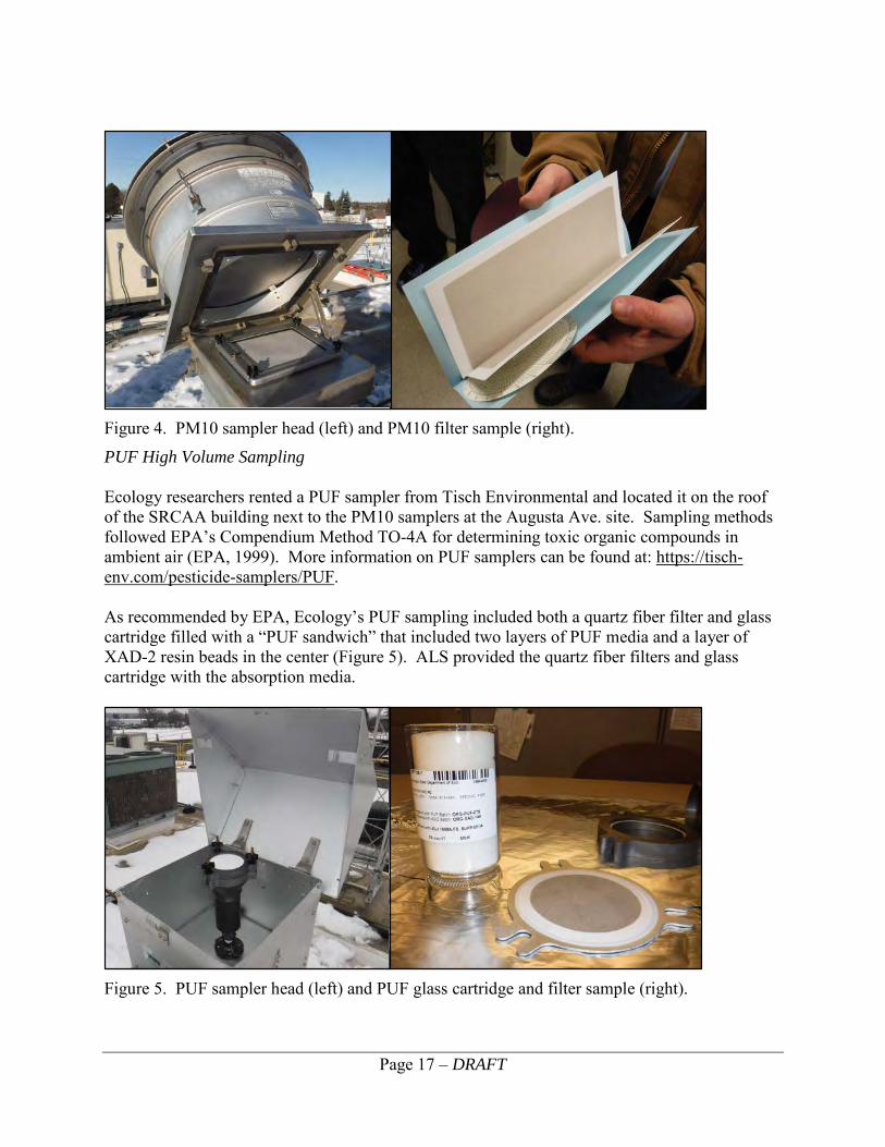
A proof-of-concept study for dry deposition collection methods was conducted in late January through mid-February of 2017 at the Augusta Ave. (urban/industrial) monitoring station. The objective was to test the efficacy of using PM10 (particulate matter ≤10 microns) filters from high-volume sampling for PCB analysis compared to high volume polyurethane foam (PUF) sampling. Since SRCAA samples PM10 every six days at the Augusta site and has several years’ worth of archived filters, the goal was to see if these archived samples could provide any useful PCB trend information. Neither the PM10 nor the PUF samples from the winter 2017 proof-of-concept study conducted were deemed useable for the purposes of reporting accurate PCB results. The PUF samples had significant background contamination in the PUF/XAD-2 sampling media prepared by the laboratory. The PM10 filters showed poor recovery of PCBs, showing that they could not be used to provide meaningful PCB data. The analytical laboratory, ALS Global (ALS), offered to conduct an in-kind second round of PUF sampling due to the contamination issues with the PUF/XAD-2 sampling media. Thus, Ecology conducted a second round of PUF sampling at the Augusta Ave. monitoring site on several dates in summer of 2017. The PM10 component was not included in the additional summer sampling since it proved to not be useful for PCB analysis. All of the PM10 and PUF sampling events were conducted as 24-hour events. For the proof-of- concept study, PM10 and PUF sampling was performed in tandem during three events on January 31, February 6, and February 17, 2017. The summer PUF sampling was carried out during three 24-hour events that straddled two calendar days starting at 1:00 pm on the first day. The dates were August 29-30, 2017, September 2-3, 2017, and September 5-6, 2017. PM10 High Volume Sampling SRCAA follows the procedures laid out by the Ecology’s Air Quality Program (AQP) for High Volume PM10 sampling (Rauh, 2003). PM10 high-volume air samplers are constructed according to the guidelines outlined in 40 CFR appendix J to part 50 and the collection method is designated as a federal reference method (FRM) under designation number 0202-141. More information on PM10 samplers can be found at: https://tisch-env.com/high-volume-air-sampler/pm10. SRCAA staff run their PM10 samplers for a 24-hour period every 6 days according to EPA’s established schedule. They archive each 8 x 10 inch quartz microfiber PM10 filter sample (Figure 4). The PM10 sampler’s flow rate is 1.13 m3/min and, with a sample run time of 24 hours, the total volume of air sampled is about 1,627 m3. The 24-hour average PM10 mass concentration for the Augusta Ave. monitoring station has had a mean value of 21 ug/m3 for the past five years. This averages out to approximately 0.03 grams of mass per filter (M. Rowe, personal communication).

Page 17 – DRAFT

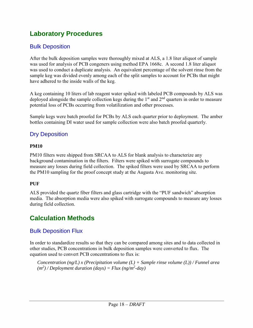
Figure 4. PM10 sampler head (left) and PM10 filter sample (right). PUF High Volume Sampling Ecology researchers rented a PUF sampler from Tisch Environmental and located it on the roof of the SRCAA building next to the PM10 samplers at the Augusta Ave. site. Sampling methods followed EPA’s Compendium Method TO-4A for determining toxic organic compounds in ambient air (EPA, 1999). More information on PUF samplers can be found at: https://tisch-env.com/pesticide-samplers/PUF. As recommended by EPA, Ecology’s PUF sampling included both a quartz fiber filter and glass cartridge filled with a “PUF sandwich” that included two layers of PUF media and a layer of XAD-2 resin beads in the center (Figure 5). ALS provided the quartz fiber filters and glass cartridge with the absorption media.

Figure 5. PUF sampler head (left) and PUF glass cartridge and filter sample (right).

Page 18 – DRAFT

Laboratory Procedures Bulk Deposition After the bulk deposition samples were thoroughly mixed at ALS, a 1.8 liter aliquot of sample was used for analysis of PCB congeners using method EPA 1668c. A second 1.8 liter aliquot was used to conduct a duplicate analysis. An equivalent percentage of the solvent rinse from the sample keg was divided evenly among each of the split samples to account for PCBs that might have adhered to the inside walls of the keg. A keg containing 10 liters of lab reagent water spiked with labeled PCB compounds by ALS was deployed alongside the sample collection kegs during the 1st and 2nd quarters in order to measure potential loss of PCBs occurring from volatilization and other processes. Sample kegs were batch proofed for PCBs by ALS each quarter prior to deployment. The amber bottles containing DI water used for sample collection were also batch proofed quarterly. Dry Deposition PM10

PM10 filters were shipped from SRCAA to ALS for blank analysis to characterize any background contamination in the filters. Filters were spiked with surrogate compounds to measure any losses during field collection. The spiked filters were used by SRCAA to perform the PM10 sampling for the proof concept study at the Augusta Ave. monitoring site. PUF

ALS provided the quartz fiber filters and glass cartridge with the “PUF sandwich” absorption media. The absorption media were also spiked with surrogate compounds to measure any losses during field collection.

Calculation Methods Bulk Deposition Flux In order to standardize results so that they can be compared among sites and to data collected in other studies, PCB concentrations in bulk deposition samples were converted to flux. The equation used to convert PCB concentrations to flux is:

Concentration (ng/L) x (Precipitation volume (L) + Sample rinse volume (L)) / Funnel area (m2) / Deployment duration (days) = Flux (ng/m2-day)

Page 19 – DRAFT

Dry Deposition Flux The PUF sampler used for the study was the TE-1000 rented from Tisch Environmental. The sampler came with a calibrated orifice transfer standard that was used to calibrate the sampler onsite prior to sampling. The calculation for determining sampler flow is outlined in EPA’s Compendium Method TO-4A for determining toxic organic compounds in ambient air (EPA, 1999). We used a spreadsheet developed by Ecology’s Air Quality Program (AQP) Northwest Regional Office (NWRO) to calculate sampler flow (m3/minute), air sample volume (m3) and PCB flux (pg/m3). See Appendix A for the calculation spreadsheets. Average air temperature and pressure for each monitoring event was downloaded from Weather Underground for the nearby Felts Field weather station. PCB Summing For summing of totals, non-detected results were assigned a value of zero. If only non-detected results comprised the total value, then the final total result was simply reported as “ND” for not detected. Sample totals were assigned a qualifier of “J” (estimated) if more than 10% of the result concentrations are composed of results containing “J” qualifiers. Qualifier Definitions

Definitions for the data quality qualifiers are as follows: J: Analyte was positively identified. The reported result is an estimate. NJ: There is evidence that the analyte is present in the sample. Reported result for the

tentatively identified analyte is an estimate. U: Analyte was not detected at or above the reported result. UJ: Analyte was not detected at or above the reported estimate NUJ: There is evidence the analyte is present in the sample. Tentatively identified analyte was

not detected at or above the reported estimate. Censoring for Method Blank Contamination Individual PCB congeners were censored using three different censoring levels for PCB contamination present in the laboratory method blank. Censoring congeners against positively identified compounds in the laboratory method blank (MB) results accounts for any PCB contamination directly from the analytical process. Homologue totals and total PCBs were calculated using the three different MB censoring levels for congeners:

1. A congener will be considered as a non-detect (“U”, “UJ” or “NUJ”) if the concentration is less than 3 times the concentration of the associated MB.

2. Same, but with < 5 times the MB.

3. Same, but with < 10 times the MB.

Results for all three censoring levels are shown Appendix B. Censoring at < 3 times the MB is used for reporting in the Results and Discussion sections of this report.

Page 20 – DRAFT

Waste to Energy Facility Plume Dispersion Modeling Ecology’s Air Quality Program (AQP) conducted plume dispersion modeling and analysis of the City of Spokane’s Waste to Energy (WTE) facility as a possible source of PCBs in atmospheric deposition to the Spokane area. AQP utilized the American Meteorological Society (AMS)/-U.S. Environmental Protection Agency (EPA) Regulatory Model (AERMOD; v16216r) to simulate the transport, dispersion and deposition of PCBs released from WTE from May 11, 2016 to May 11, 2017 (PCB bulk deposition study time frame). AQP also assessed the representativeness of this one-year period by running AERMOD for 5-years using meteorological data from 2011 – 2015. Emission data were obtained from reports of source sampling run tests performed from 2011 to 2017. Other important pollutant and building information were taken from 1991 and 2001 dispersion modeling done for health risk assessment studies (ETI, 1991; PTC, 2001). Meteorological data were obtained from the Spokane International Airport. AERMOD simulated concentrations and deposition (total, dry and wet) estimates covered a 900 km2 domain, centered on the emission source at the WTE. Model outputs averaged over 24-hour, monthly and the whole period averaging time were compared against the 1-year field study period for three monitoring sites. Methods are fully discussed in the modeling and analysis report (Appendix D.)

Page 21 – DRAFT

Data Quality The study data were reviewed by the report authors, analytical chemists and Manchester Environmental Laboratory (MEL). MEL provided a Stage 4 validation of the data. The majority of the study data were found to meet the laboratory measurement quality objectives (MQOs) outlined in the QA Project Plan (Era-Miller and Wong, 2016) and shown in Table 2. These MQOs are specific to method EPA 1668c and pertain to both the dry and bulk deposition (aqueous) sample matrices.

Table 2. Measurement Quality Objectives (MQOs) for the Study.

Lab Control

Samples (% Recovery)

Lab Duplicate Samples (RPD)

Surrogate Recoveries

(% Recovery)

MQO limits 50 – 150† ≤50% 25 – 150a Sampling Event Percent of Data Meeting MQOs

Bulk Dep. – Qtr. 1 100% 100% 100%

Bulk Dep. – Qtr. 2 100% 99% 88%

Bulk Dep. – Qtr. 3 100% NA 100%

Bulk Dep. – Qtr. 4 56% NC 99% Dry Dep. – Summer 93% NA 97%

† Per Method for Ongoing Precision and Recovery (OPR), internal standards, and labeled compounds a labeled congeners NC: not calculated due to the low number of detections in the duplicate sample NA: data not analyzed for EPA: U.S. Environmental Protection Agency RPD: Relative percent difference

Bulk Deposition Multiple types of bulk deposition sampling system quality assurance/quality control (QA/QC) samples were analyzed during the study. These included proofing of sampling containers and laboratory reagent water, analysis of laboratory method blanks, sampling equipment blanks, field replicates, field spike samples and collection efficiency wipe samples. Proofing After ALS decontaminated the 20 liter sample kegs, additional solvent was rinsed through all the kegs, composited, then analyzed for PCBs. The 1 liter amber glass bottles with laboratory reagent water were also proofed for PCBs. The amber bottles were used to transport the laboratory reagent water for bulk deposition sample collection. The total PCB results for the proofed containers along with their associated laboratory method blank (MB) results are shown in Table 3. These concentrations were relatively low compared to the equipment blank and bulk

Page 22 – DRAFT

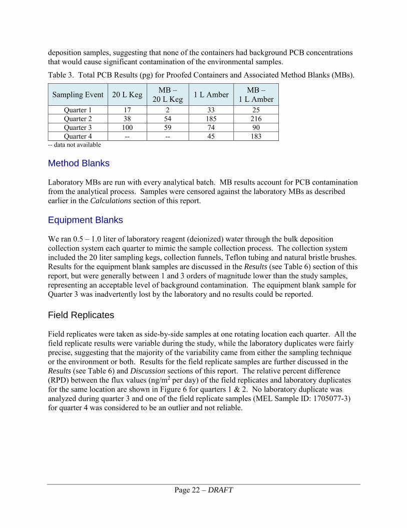
deposition samples, suggesting that none of the containers had background PCB concentrations that would cause significant contamination of the environmental samples.

Table 3. Total PCB Results (pg) for Proofed Containers and Associated Method Blanks (MBs).

Sampling Event 20 L Keg MB – 20 L Keg 1 L Amber MB –

1 L Amber Quarter 1 17 2 33 25 Quarter 2 38 54 185 216 Quarter 3 100 59 74 90 Quarter 4 -- -- 45 183

-- data not available Method Blanks Laboratory MBs are run with every analytical batch. MB results account for PCB contamination from the analytical process. Samples were censored against the laboratory MBs as described earlier in the Calculations section of this report. Equipment Blanks We ran 0.5 – 1.0 liter of laboratory reagent (deionized) water through the bulk deposition collection system each quarter to mimic the sample collection process. The collection system included the 20 liter sampling kegs, collection funnels, Teflon tubing and natural bristle brushes. Results for the equipment blank samples are discussed in the Results (see Table 6) section of this report, but were generally between 1 and 3 orders of magnitude lower than the study samples, representing an acceptable level of background contamination. The equipment blank sample for Quarter 3 was inadvertently lost by the laboratory and no results could be reported. Field Replicates Field replicates were taken as side-by-side samples at one rotating location each quarter. All the field replicate results were variable during the study, while the laboratory duplicates were fairly precise, suggesting that the majority of the variability came from either the sampling technique or the environment or both. Results for the field replicate samples are further discussed in the Results (see Table 6) and Discussion sections of this report. The relative percent difference (RPD) between the flux values (ng/m2 per day) of the field replicates and laboratory duplicates for the same location are shown in Figure 6 for quarters 1 & 2. No laboratory duplicate was analyzed during quarter 3 and one of the field replicate samples (MEL Sample ID: 1705077-3) for quarter 4 was considered to be an outlier and not reliable.

Page 23 – DRAFT

RPD: relative percent difference dup: laboratory duplicate Figure 6. Difference between tPCB flux values for field replicates and laboratory duplicates.

Sample Outlier Sample 1705077-3 (from the Turnbull station for quarter 4) had a tPCB concentration that was contrary to the first three quarters where results were always the lowest for Turnbull, which is the regional background site. The Turnbull field replicate for quarter 4 (1705077-4) followed previous observations, having lower tPCB concentrations than the other monitoring sites. Congener distributions in sample 1705077-3 were also different from any of the samples in the study. For these reasons, we consider sample 1705077-3 to be an outlier and do not consider it in our interpretation of regional atmospheric deposition of PCBs. Field Spikes Field spikes were deployed during the first and second quarter of the study to measure potential loss of PCBs occurring from volatilization and other processes such as adhesion to the sample kegs during deployment. The field spike sample recoveries were acceptable and ranged from 54 – 117%, indicating that losses due to a three month deployment in the field were not a concern. Efficiency Wipes Solvent-soaked wipes were used to measure bulk deposition removal efficiency on the stainless steel sample funnels directly after collection in the field. The PCB mass on the wipe is compared to the PCB mass in the associated sample. Removal efficiencies of PCBs from the surface of the sample collection bowls ranged from 96.4 – 99.7 % (Table 4). Results for the wipes and field samples in Table 4 were censored against their batch-specific laboratory MBs at 3x.

Result 1 Result 2 RPD

Sample Replicate 35%

Replicate Replicate (dup) 12%

Result 1 Result 2 RPD

Sample Replicate 62%

Replicate Replicate (dup) 5%

Page 24 – DRAFT

Table 4. Bulk deposition collection bowl PCB removal efficiency.

Sampling Quarter Station tPCB Mass

(pg) Wipe tPCB Mass (pg) Sample

PCB removal Efficiency (%)

2 Monroe 40 14,964 99.7 3 Monroe 426 28,277 98.5 3 Turnbull 118 24,542 99.5 3 Turnbull 127 20,954 99.4 4 Augusta 426 11,807 96.4 4 Monroe 359 10,172 96.5

Dry Deposition As described earlier in the Methods section of this report, results from both the PM10 and PUF samples from the winter 2017 proof of concept study were deemed unusable. The following data quality discussion refers only to the summer 2017 PUF sampling. QA/QC samples for the PUF sampling included proofing of PUF/XAD-2 absorption material and analysis of a field blank and laboratory method blank. The concentrations of tPCBs in all the QA/QC samples were orders of magnitude lower than the high concentrations found in the environmental samples (Table 5). The field blank sample, which accounts for background contamination from the entire sampling system (field and laboratory), was two orders of magnitude lower than the environmental samples.

Table 5. Dry deposition QA/QC results compared to field samples.

Sample Type tPCB Mass (pg) PUF/XAD-2 proof 280 Method blank 33 Field blank 1,240 Sample – Event 1 213,000 Sample – Event 2 189,000 Sample – Event 3 114,000

Waste to Energy Facility Plume Dispersion Modeling Ecology’s Air Quality Program (AQP) provided internal peer review of the modeling results. The American Meteorological Society (AMS)/-U.S. Environmental Protection Agency (EPA) Regulatory Model (AERMOD; v16216r) modeling system was used for the modeling and all input data came from published reports or peer reviewed sources. See Appendix D for full report.

Page 25 – DRAFT

Results

Bulk Deposition Total PCB results are provided in Table 6 by mass (pg), concentration (pg/L – part per quadrillion and ng/L – part per trillion) and flux rate (ng/m2 per day). Equipment blank, field replicate and laboratory duplicate results are also included. PCB results in Table 6, Figure 7 and the body of the report were censored on a per congener basis at 3 times the laboratory method blank (MB). An Excel spreadsheet showing the full congener data censored at 3, 5, and 10 times the MB along with homologue pattern graphs shown with censoring at 3 and 10 times the MB are presented in Appendix B.

Table 6. Total PCB Bulk Deposition Results.

MEL ID: Manchester Environmental Laboratory sample ID rep: replicate sample deployed side-by-side in the field Dup: duplicate aliquot sample taken at the laboratory * Turnbull sample 1705077-3 is an outlier Figure 7 shows a general trend of increasing total PCB flux values moving from Turnbull, the regional background site, to Monroe (urban – residential) and then to Augusta (urban – industrial). Field replicate and laboratory duplicate values were averaged for Figure 7. Augusta had the highest total PCB flux for the study during the second quarter (mid-August to mid-November, 2016) with an average of 10.8 ng/m2 per day (Figure 7). The mean rural and urban – residential values from a study conducted in the Duwamish River Watershed by King County in 2011 – 2013 are displayed in Figure 7 for comparison (King County, 2015).

Deployment RetrievaltPCB

Mass (pg)Sample

volume (L)tPCB pg/L

tPCB ng/L

1 Equipment Blank 1608070-1 5/6/16 -- -- 1.0 957 0.95 1007 1.0 --1 Turnbull 1608070-4 5/11/16 8/11/16 90 8.1 3099 7.63 406 0.4 0.411 Monroe 1608070-2 5/12/16 8/10/16 90 7.3 11242 6.77 1661 1.7 1.511 Monroe (rep) 1608070-3 5/12/16 8/10/16 90 7.3 7874 6.81 1156 1.2 1.061 Monroe (rep) Dup -- 5/12/16 8/10/16 90 7.3 8864 6.81 1302 1.3 1.191 Augusta 1608070-5 5/11/16 8/11/16 89.8 8.3 20331 7.8 2607 2.6 2.712 Equipment Blank 1611056-1 8/16/16 -- -- 0.47 923 0.47 1964 2.0 --2 Turnbull 1611056-3 8/11/16 11/16/16 96.7 17.3 7129 16.8 425 0.4 0.852 Monroe 1611056-2 8/10/16 11/16/16 98.1 16.7 14964 16.2 925 0.9 1.772 Augusta 1611056-4 8/11/16 11/16/16 97.1 15.5 120034 15.0 8008 8.0 14.32 Augusta (rep) 1611056-5 8/11/16 11/16/16 97.1 15.7 63183 15.2 4168 4.2 7.552 Augusta (rep) Dup -- 8/11/16 11/16/16 97.1 15.7 60227 15.2 3962 4.0 7.203 Turnbull 1702021-3 11/16/16 2/15/17 91.2 10.8 24542 10.3 2394 2.4 3.173 Turnbull (rep) 1702021-5 11/16/16 2/15/17 91.2 10.8 20954 10.3 2030 2.0 2.713 Monroe 1702021-2 11/16/16 2/15/17 90.8 11.6 28277 11.1 2554 2.6 3.663 Augusta 1702021-1 11/16/16 2/16/17 91.8 11.3 30329 11.3 2675 2.7 3.714 Equipment Blank 1705077-1 2/23/17 -- -- 0.54 94 0.5 174 0.2 --4 Turnbull* 1705077-3 2/15/17 5/11/17 84.9 16.4 37231 15.86 2347 2.3 5.084 Turnbull (rep) 1705077-4 2/15/17 5/11/17 84.9 16.8 452 16.28 28 0.03 0.064 Turnbull (rep) Dup -- 2/15/17 5/11/17 84.9 16.8 446 16.28 27 0.03 0.064 Monroe 1705077-2 2/15/17 5/11/17 85.0 17.4 10172 16.9 602 0.6 1.384 Augusta 1705077-5 2/16/17 5/11/17 84.1 13.8 11807 13.3 888 0.9 1.64

Quarter Sample Name MEL ID DaysTotal

Volume (L)Flux

ng/m2-day

Page 26 – DRAFT

Figure 7. Bulk deposition Total PCB flux results.

Equipment Blank Correction As previously stated, bulk deposition PCB congener results were censored at 3 times the laboratory method blank (MB) to account for background PCB contamination from the laboratory. In order to characterize the possible effects of background contamination from sample collection and field activities, the equipment blank total PCB mass concentrations (pg) were subtracted from the sample total PCB mass concentrations prior to flux calculations. Table 7 shows that this blank correction exercise generally did not substantially reduce flux values compared to the non-blank corrected flux values indicating that the majority of the PCBs in the samples were from the environment and not the sampling system. Since there was no useable equipment blank result for the 3rd quarter of sampling, an average of the blank results for the other quarters was used.

Table 7. Bulk Deposition Flux with and without Equipment Blank Correction.

BC: blank-corrected result

0.0

2.0

4.0

6.0

8.0

10.0

12.0

Turnbull Monroe Augusta

Bulk Deposition Flux ng/m2-day

Qtr 1 Qtr 2 Qtr 3 Qtr 4

mean Rural (Enumclaw)

mean Urban/Residential (Beacon Hill)

Result BC Result BC Result BC Result BCTurnbull 0.4 0.3 69% 0.9 0.7 87% 2.9 2.9 97% 0.06 0.05 79%Monroe 1.3 1.2 90% 1.8 1.7 94% 3.7 3.6 98% 1.4 1.4 99%Augusta 2.7 2.6 95% 10.9 10.8 99% 3.7 3.6 98% 1.6 1.6 99%

SiteFlux ng/m2 -day Flux ng/m2 -day Flux ng/m2 -day% of

Result% of

Result% of

Result

Qtr 1 Qtr 2 Qtr 3 Qtr 4Flux ng/m2 -day % of

Result

Page 27 – DRAFT

Environmental Data Weather patterns and other environmental conditions have a profound effect on atmospheric deposition (King County, 2015). Environmental variables include precipitation, temperature, wind direction, wind speed, particulate matter in the air, landscape and landuse. Precipitation, temperature, wind and air particulate conditions during the study period are presented below. Precipitation

Quarterly bulk deposition sample volumes (liters) and precipitation data (inches) from Felts Field airport are shown in Table 8. Felts Field is located 3 miles northeast of the Augusta Ave. monitoring location. Precipitation (inches) was estimated for all three monitoring locations based on sample volumes. Total precipitation for the study period was approximately 24 inches at both Felts Field and at the Spokane International Airport. The average precipitation for Spokane is about 16.5 inches annually. The month of October 2016, was the wettest month ever recorded for Spokane (NOAA, 2016). Table 8. Quarterly precipitation during bulk deposition collection.

*Precipitation (inches) for the three monitoring locations are estimates calculated from precipitation volume. The Felts Field data are actual measured data. Temperature

Daily high and low temperatures at Felts Field Airport during the bulk deposition study period are shown with the historical daily average high and low temperatures for Spokane in Figure 8. The highest high was 99○ F and the lowest low was -1○ F. Daily temperature statistics and daily precipitation from the Spokane International Airport are graphed together in Figure 9 to show the combined seasonal variability of these two major environmental factors during quarterly bulk deposition sampling.

Precipitation Volume (L) precip. (in)*

Precipitation Volume (L) precip. (in)*

Precipitation Volume (L) precip. (in)*

Precipitation Volume (L) precip. (in)*

Turnbull 7.63 3.38 16.79 7.44 10.25 / 10.32 4.54 / 4.57 15.86 / 16.28 7.02 / 7.21Monroe 6.77 / 6.81 3.00 / 3.02 16.18 7.17 11.07 4.90 16.90 7.48Augusta 7.80 3.45 14.99 / 15.16 6.64 / 6.71 11.34 5.02 13.30 5.89Felts Field -- 3.53 -- 7.50 -- 5.92 -- 7.01

Quarter 42/16/17 - 5/10/17

Location

Quarter 15/11/16 - 8/11/16

Quarter 28/12/16 - 11/17/16

Quarter 311/18/16 - 2/15/17

Page 28 – DRAFT

Figure 8. Daily high and low temperatures at Felts Field Airport during bulk deposition collection along with historical daily high and low temperatures for Spokane (data for Felts Field from Weather Underground and historical data from Intellicast.com).

Figure 9. Temperature and precipitation at the Spokane International Airport during bulk deposition collection (data from NOAA).

0

10

20

30

40

50

60

70

80

90

100

5/11/16 6/11/16 7/11/16 8/11/16 9/11/16 10/11/16 11/11/16 12/11/16 1/11/17 2/11/17 3/11/17 4/11/17 5/11/17

study high study low historical high historical low

Quarter 1 Quarter 2 Quarter 4Quarter 3Te

mpe

ratu

re (F

◦ )Te

mpe

ratu

re F○

Prec

ipita

tion

Inch

es

Quarter 1 Quarter 2 Quarter 4Quarter 3

0

0.1

0.2

0.3

0.4

0.5

0.6

0.7

0.8

0.9

1

-20

0

20

40

60

80

100

120

Temp. AVG MAX MIN Precip.

Page 29 – DRAFT

Wind Direction and Speed

Wind direction and wind speed in the Spokane area varies throughout the year, though wind direction is predominately from the southwest. Wind direction during the quarterly bulk deposition sampling followed this pattern. Quarterly wind roses for Augusta Ave. monitoring site, the Spokane International Airport and Felts Field Airport are shown in Appendix C, figures C-1 through C-3.

PM2.5 and PM10

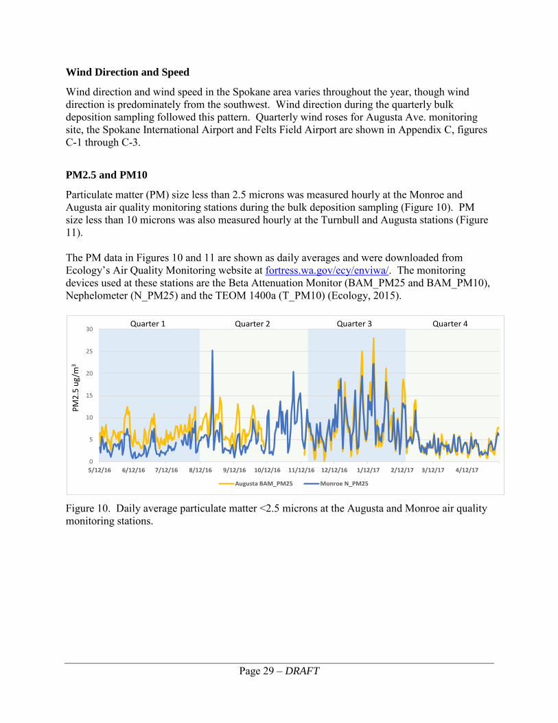
Particulate matter (PM) size less than 2.5 microns was measured hourly at the Monroe and Augusta air quality monitoring stations during the bulk deposition sampling (Figure 10). PM size less than 10 microns was also measured hourly at the Turnbull and Augusta stations (Figure 11). The PM data in Figures 10 and 11 are shown as daily averages and were downloaded from Ecology’s Air Quality Monitoring website at fortress.wa.gov/ecy/enviwa/. The monitoring devices used at these stations are the Beta Attenuation Monitor (BAM_PM25 and BAM_PM10), Nephelometer (N_PM25) and the TEOM 1400a (T_PM10) (Ecology, 2015).

Figure 10. Daily average particulate matter <2.5 microns at the Augusta and Monroe air quality monitoring stations.

Quarter 1 Quarter 2 Quarter 4Quarter 3

PM2.

5 ug

/m3

0

5

10

15

20

25

30

5/12/16 6/12/16 7/12/16 8/12/16 9/12/16 10/12/16 11/12/16 12/12/16 1/12/17 2/12/17 3/12/17 4/12/17

Augusta BAM_PM25 Monroe N_PM25

Page 30 – DRAFT

Figure 11. Daily average particulate matter <10 microns at the Turnbull and Augusta air quality monitoring stations.

Dry Deposition (PUF Sampling) Proof-of-Concept Study A proof-of-concept study for dry deposition collection methods was conducted in late January through mid-February of 2017 at the Augusta Ave. (urban/industrial) monitoring station. The objective was to test the efficacy of using PM10 filters from high-volume sampling for PCB analysis compared to the more traditional method of sampling atmospheric PCBs through use of high volume PUF sampling. Since SRCAA samples PM10 every six days at the Augusta site and has several years’ worth of archived filters, we wanted to see if these archived samples could provide any useful PCB trend information. The PM10 filter samples had extremely low or no recovery of the mono- through hepta- chlorinated congeners, suggesting that they could not be used to provide meaningful PCB data. EPA’s Compendium Method TO-4A for determining toxic organic compounds in ambient air supports this finding in stating that the volatility of compounds like PCBs prevents efficient collection on filter media alone (EPA, 1999). Thus, EPA recommends using both a filter and PUF media together for efficient capture. In addition to the low recovery of congeners in the PM10 samples, there was significant background contamination in the PUF/XAD-2 sampling media which overwhelmed the signal of the di- through penta- chlorinated congeners in the PUF samples. Consequently, the PUF samples from the winter 2017 (proof-of-concept) sampling also did not generate useable PCB data.

Quarter 1 Quarter 2 Quarter 4Quarter 3PM

10 u

g/m

3

0

10

20

30

40

50

60

70

80

90

5/12/16 6/12/16 7/12/16 8/12/16 9/12/16 10/12/16 11/12/16 12/12/16 1/12/17 2/12/17 3/12/17 4/12/17

Turnbull BAM_PM10 Augusta T_PM10

Page 31 – DRAFT

Summer PUF Sampling Ecology conducted a second round of PUF sampling in summer 2017. Three 24-hour high volume PUF samples were obtained at the Augusta Ave. monitoring (urban – industrial) site in late August through early September. Total PCB concentrations (pg/m3) are shown in Table 9. Table 9. Total PCB results for summer 2017 PUF dry deposition sampling.

Sampling Event 1 2 3 2017 dates 8/29 - 8/30 9/2 - 9/3 9/5 - 9/6

Sample Volume (m3) 242 297 252 tPCB Mass (pg) 212,734 189,662 114,373 tPCB Concentration pg/m3 880 639 454

All three PUF sampling events coincided with a period of poor air quality from high PM2.5 levels due to numerous regional wildfires. The Spokane Regional Clean Air Agency (SRCAA) stated that the 2017 wildfire season was officially the worst that they have on record and that the Spokane-area saw its highest concentrations of PM2.5 over the longest duration (SRCAA, 2017). Figure 12 shows the daily average PM2.5 levels from June 1st to October 1st 2017. All three PUF sampling events occurred when PM2.5 levels were elevated, but the third sampling event captured peak PM2.5 conditions.

Figure 12. Daily average PM2.5 levels during the 2017 fire season with PUF sampling events.

Figure 13 is a graph of hourly PM2.5 that occurred during each PUF sampling event and shows the condition of the sample filters after each event. Sampling event 3 had the highest PM2.5 levels, but the lowest tPCB concentrations compared to events 1 and 2. Sampling Event 1 had

0

20

40

60

80

100

120

140

160

180

200

6/1/2017 7/1/2017 8/1/2017 9/1/2017 10/1/2017

PM2.

5 ug

/m3

Event 1

Event 2

Event 3

Page 32 – DRAFT

the highest tPCB concentration, about double that of Event 3, indicating that increased PM2.5 levels from wildfire smoke didn’t necessarily correlate with increased concentrations of PCBs.

Figure 13. PM2.5 Data (top) and pictures of PUF filters after sampling wildfire smoke (bottom). Congener patterns for the PUF sampling events are presented in Figure 14. Sampling events 1 and 2 appear to have identical patterns. Event 3 is similar to the first two events except for congeners -001 through -004 and congener -038 which are circled in red on Figure 14. This suggests that all three samples came predominately from the same source.

Event 1 Event 2 Event 3

0

50

100

150

200

250

PM2.

5 u

g/m

3

Time

Event 1 (Aug 29 - 30)

Event 2 (Sept 2 - 3)

Event 3 (Sept 5 - 6)

Page 33 – DRAFT

Figure 14. PCB Congener patterns in wildfire smoke-dominated PUF samples. Areas of dissimilar patterns are circled in Event 3.

Waste to Energy Facility PCB Plume Dispersion Modeling Ecology’s Air Quality Program (AQP) conducted plume dispersion modeling and analysis of the City of Spokane’s Waste to Energy (WTE) facility as a possible source of PCBs in atmospheric deposition to the Spokane area. Results are summarized below. See Appendix D for the full modeling report. Modeling results for the 1-year PCB bulk deposition study (Figure 15a) and a 5-year case study (Figure 15b) show that highest annual PCB concentrations (pg/m3) were located over the northeastern, south, and the west-southwestern region in about a 2-mile radius from the emission source. As can be seen from the figures, the two urban air quality monitoring sites of Augusta and Monroe are outside the areas with the highest concentrations. In general, the 5-year modeling case shows concentrations over a larger area than the 1-year field study case, while the overall plume distribution is similar. Quantitatively, the 5-year modeling results are about 16% higher in concentration and 20% higher in bulk deposition than the 1-year field study period modeling results (Table 10). The comparison between 1-year and 5-year model runs highlights the importance of using a longer period of meteorological data to avoid basing decisions on less representative conditions.

Event 1

Event 2

Mas

s in

Pic

ogra

ms

Lesser Chlorinated More Chlorinated

Event 3

Page 34 – DRAFT

(a) (b)

Figure 15. Modeled average annual PCB concentration distribution from the Spokane WTE stack. (a) For May 11, 2016 to May 11, 2017 field measurement case study. (b) Regulatory 5-year modeling study period of January 2011 to December 2015. Coordinates are in UTM (m) and concentration is in picograms per cubic meter (pg/m3).

Table 10. AERMOD results of concentration and deposition for the 24-hour averaging period for PCBs average particle density and average emission rate at WTE.

Modeling Time

Concentration (pg/m3)

Total Deposition

(ng/m2)

Dry Deposition

(ng/m2)

Wet Deposition

(ng/m2) 1 year 2.431 11.056 10.987 6.204 5 years 2.826 13.277 13.273 11.389

The qualitative plots of both the study and the 5-year periods show that total (bulk) deposition across the domain has a similar distribution (Figures 16a and 16b). The modeled deposition over the Spokane urban sites of Augusta and Monroe are very low compared to the measured concentrations and fluxes at the monitoring sites. From Figure 16a, the Augusta site is situated within the 8 – 10 ng/m2 per year (0.02 – 0.03 ng/m2 per day) contour of modeled deposition values, while Monroe is within the 20 – 50 ng/m2 per year (0.05 – 0.14 ng/m2 per day) contour. On the other hand, observed bulk deposition values at these two sites vary from 1.2 – 10.9 ng/m2 per day (see Table 11).

Page 35 – DRAFT

(a) (b)

Figure 16. Modeled average annual total (bulk) deposition distribution from the Spokane WTE stack. (a) For May 11, 2016 to May 11, 2017 field measurement case study. (b) Regulatory 5-year modeling study period of January 2011 to December 2015. Coordinates are in UTM (m) and deposition is in nanograms per square meter (ng/m2).

Table 11. AERMOD modeled and observed quarterly total (bulk) deposition data for three monitoring sites for the study period of 05/11/16 to 05/11/17.

Site Site Type Data Type (ng/m2 –per day)

Quarter 1 5/11/16 – 8/10/16

Quarter 2 8/11/16 – 11/16/16

Quarter 3 11/17/16 – 2/15/17

Quarter 4 2/16/17 – 5/11/17

Augusta Commercial Model 0.025 0.023 0.015 0.030 Observed 2.610 10.920 3.710 1.670

Monroe Residential Model 0.062 0.060 0.041 0.074 Observed 1.240 1.740 3.660 1.380

Turnbull Regional/ Background

Model 0.004 0.007 0.011 0.004 Observed 0.370 0.850 2.940 0.060

Page 36 – DRAFT

Discussion

Bulk Deposition of PCBs in Spokane Bulk atmospheric deposition flux can be defined as the amount of dry particles combined with particles in precipitation that are deposited on the surface of a defined area over a specific period of time (e.g., ng/m2-per day). Atmospheric flux values can be used to estimate the atmospheric loading of a chemical to land surface and eventually, via runoff processes, to surface water. The annual average flux values for the Spokane bulk deposition samples are within a similar range to the average flux values found in the same landuse types (i.e., rural, urban/commercial and urban/residential) in the Duwamish River Watershed, near Seattle (Figure 17). Because the sampling methods for the Spokane study were adapted from King County, the data between these studies is highly comparable. The main difference is that King County collected samples on a more frequent basis during the year (n = 5 – 15) and for shorter deployment periods (7 – 29 days).

Figure 17. Average total PCB flux (ng/m2 – day) values for Spokane and the Duwamish River Watershed (King County, 2015). The general trend of increasing total PCB flux values moving from Turnbull, the regional background site, to Monroe (urban/residential) and then to Augusta (urban/industrial) is not surprising as the trend of cities and urban areas having higher PCB concentrations than rural and remote areas is strongly supported by the scientific literature (Holsen, et al., 1991, Park, et al., 2001, Diamond, et al., 2010). Urban areas in general are often major sources of PCBs to the atmosphere, especially when temperatures are elevated and the wind comes urban and industrialized areas (Holsen, et al., 1991, Park, et al., 2001, King County, 2015).

0 10 20 30 40 50 60 70 80

Turbull NWR

Urban/Residential

Urban/Commercial

Rural

Urban/Residential

Urban/Comercial

Urban/Comercial

Urban/Comercial

Industrial/Urban

Urban/Transportation

Duwamish River Watershed 2011-2013(King County, 2015)

Spokane 2016-2017

Page 37 – DRAFT

Site-Specific Congener Patterns in Bulk Deposition Principle component analysis (PCA) was used to explore similarities and differences in PCB congener patterns in bulk deposition samples between monitoring sites and quarterly seasonal sampling events. The goal of PCA is to reduce the complexity of a large, multiple variable dataset without losing information. A plot of first two principal components is an effective way of showing how chemically similar samples are, where points closer together are more similar than points further away (Figure 18). There is separation between the Turnbull, Monroe and Augusta monitoring sites along PC1. This means that samples from the same individual sites naturally grouped together because they exhibited more similar congener distribution patterns. One of the Turnbull replicate samples from quarter 4, considered to be an outlier, is circled and shaded below the monitoring site groupings in Figure 18. Equipment blank samples were included in the PCA and generally did not group with the monitoring sites, confirming the Turnbull replicate as an outlier.

Figure 18. PCA ordination plot for PCB congeners in bulk deposition.

Page 38 – DRAFT

Homologue analysis of the bulk deposition samples (Appendix B, figures B-2 through B-5) indicated that more of the higher chlorinated congeners dominated at the Monroe St. and Augusta Ave. urban sites compared to the regional reference site at Turnbull. King County found similar results during their 2011 – 2013 bulk deposition studies where the rural site at Enumclaw had only small a contribution or absence of higher chlorinated congeners (> hexa-CB) compared to the suburban and urban sites (King County, 2015).

Modeled PCBs from WTE versus Measured PCBs Figure 19 compares the modeled PCBs for the Spokane WTE Facility to the measured results in bulk deposition from each of the study sites. The modeled values for the Spokane WTE Facility are less than 2% of the measured values for the four quarters of the study period. In other words, the monitored deposition values are about two orders of magnitude higher than the modeled values for the WTE Facility. These quantitative and qualitative comparisons show that the PCB contribution from the Spokane WTE Facility is very low. Past AERMOD sensitivity analysis studies suggested that the model generally overestimates observations, especially during calm and/or low wind speeds (Perry et al., 2005, Duoxing et al., 2007). Therefore the modeling results are likely upper bounds of what the Spokane WTE could contribute to the observed deposition, implying that there must be other contributing PCB sources in the region.

Figure 19. Comparison of quarterly bulk deposition modeling of the Spokane WTE Facility and the results for quarterly total PCB monitoring at three sites. Note logarithmic scale for y axis. (Q1 = 5/11/2017 – 8/10/2016; Q2 = 8/11/2016 – 11/16/2017; Q3 = 11/17/2016 – 2/15/2017; Q4 = 2/16/2017 – 5/11/2017).

Page 39 – DRAFT

Contribution of Atmospheric PCBs to Stormwater in the Cochran Basin One of the questions that the Spokane PCB atmospheric deposition study sought to address was: How much of the PCB loading in urban stormwater from Spokane comes from atmospheric sources? Can data from this project be used in concert with PCB data from the City of Spokane’s stormwater basin monitoring program to estimate this loading? We didn’t have time to address this question for the report, however it could still be done as a future effort. The Monroe St. air quality monitoring station is located within the City of Spokane’s Cochran stormwater basin. The City collected and analyzed PCB congeners and flow in the Cochran basin four times during the bulk atmospheric deposition study (2016 – 2017) as part of their stormwater monitoring program (Donovan, 2018, City of Spokane, 2015). PCB bulk deposition flux data from the Monroe St. station could be used to estimate the atmospheric contribution of PCBs to stormwater in the Cochran basin. Any such modeling results would be estimates with a high level of uncertainty, but could provide some useful data regarding the general impact of atmospheric PCBs to stormwater.

PCBs in Wildfire Smoke The intent of conducting additional dry deposition monitoring at Augusta in summer 2017 was to replace sampling for the compromised samples collected in winter 2017 (as part of the proof-of-concept study). In addition, we decided that having some high quality dry deposition data for the Spokane area would help to fill the data gap regarding PCBs in atmospheric deposition. The Augusta Ave. monitoring location represents an urban-commercial landuse and airshed. However, the dry deposition samples collected in summer 2017 at Augusta Ave. may be more representative of regional wildfire inputs. A scientific literature search revealed little information on PCBs in wildfire smoke. However, one study from Svalbard Norway found significant enhancements of PCBs in atmospheric samples taken in July 2014 when a large plume of smoke from boreal forest fires in Alaska and Canada traveled over Svalbard (Eckhardt et al., 2007). They only analyzed for 32 congeners however, making it difficult to compare congener patterns between the Svalbard study and Spokane study. To provide context for the wildfire smoke-dominated dry deposition data at the Augusta Ave. site, data were compared with tPCB concentrations from several other urban areas in the northeastern United States (Figure 20). PCBs in the wildfire-smoke dominated samples appear to be generally higher than PCBs in remote, rural and suburban areas, but lower than PCBs in the highly urbanized Chicago area (Hoff et al., 1994, Franz and Eisenreich, 1998, Tasdemir et al., 2004).

Page 40 – DRAFT

Figure 20. Total PCB concentrations in Spokane dry deposition compared to other states.

Air Mass Movement Back trajectories of the air masses moving over the Augusta Ave. sampling site during the sum-mer 2017 PUF sampling events were modeled by AQP using the National Oceanic and Atmos-pheric Administration’s (NOAA) HYSPLIT model (Stein, et al., 2015; Rolph, et al., 2017). Wind roses were also created for the 24-hour PUF sampling events using AERMET wind rose products and surface wind data from the Spokane International Airport. A back trajectory shows the past path of small particles in an air mass as they move through time and space in 3 dimensions (includes vertical movement) using a model such as HYSPLIT. To-gether, back trajectories and wind roses tell a story of where air masses originate and what condi-tions may have affected deposition of atmospheric pollutants at a given place and time. A full interpretation and discussion regarding the effect that air mass movement had on the sum-mer 2017 PUF sampling PCB results is beyond the scope of the current study, however some general observations are provided below for each of the three monitoring events. Event 1 (August 29 – 30, 2017)

Figure 21 shows that the air masses located at 500 m above ground level (AGL) at the start (a) and at the end (b) of sampling Event 1 originated from the southeast corner of Washington. The vertical movement of the air mass towards the end of the sampling event (b) is one of subsidence or downward movement. Subsidence can concentrate particulates in an air mass by pushing them down towards the land surface. The wind rose (c) indicates that surface wind direction was southwesterly (flowing from the southwest) for approximately half of the time and easterly (flowing from the east) for the other half. Sampling event 1 had the highest total PCB concentrations at 880 pg/m3 (Table 8).

0 500 1000 1500 2000

Spokane Wildfire 2017 - Event 3

Spokane Wildfire 2017 - Event 2

Spokane Wildfire 2017 - Event 1

Remote: Michigan - 1993

Rural: Michigan - 1993

Rural: New York - 1993

Suburban: Minnesota - 1992

Urban: Chicago - 1995

Total PCB Concentrations pg/m3

Page 41 – DRAFT

Event 2 (September 2 – 3, 2017)

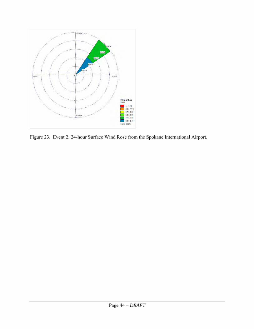
The 500 m elevation air mass trajectories (Figure 22, a and b), which were generally westerly, did not match the surface wind rose northeasterly direction (Figure 23) for sampling Event 2. The air mass trajectories were therefore plotted again, but at a 50 m elevation (Figure 22, c and d) to see if there were different wind patterns happening closer to the land surface. The 50 m and 500 m trajectories were in fact quite different, indicating major differences in wind conditions happening at the land surface versus above 500 m. Similar to air masses at 500 m for Event 1, the air masses at 50 m for event 2 also appeared to mostly originate from southeast of Spokane. Vertical data (Figure 22, b) towards the end of Event 2 showed subsidence followed by a dramatic uplift in air mass movement. Total PCBs were 639 pg/m3 for this event (Table 8). Event 3 (September 5 – 6, 2017)

Figure 24 shows that the 500 m elevation air mass trajectories for sampling Event 3 were dramatically different from Events 1 and 2 with a dominant flow from the northeast and air masses originating in Idaho, Montana and likely Canada. The wind rose (c) also shows that surface winds were northeasterly. Vertical data (a and b) indicate uplift towards both the beginning and the end of sampling. Sampling event 3 had the lowest total PCBs (454 pg/m3) and the highest PM2.5 (Table 9 and Figure 13). Did Air Mass Movement Effect PCB Concentrations and PM2.5 in Dry Deposition?

All three sampling Events exhibited highly similar congener patterns, suggesting that they came predominately from the same source. There were wildfires burning all over northwest at the time of sampling and the entire state was inundated with smoke. However, total PCB concentrations for sampling Event 1 were twice that of the Event 3 even though PM2.5 was dramatically higher in Event 3. Analysis of air mass back trajectories and wind roses from all three events suggest that the air mass for Event 3 came from the more remote areas of Idaho, Montana and Canada where wildfires were also burning at the time. So, even though PM2.5 was highest during Event 3, the source of PM2.5 was smoke from fires in remote forestland. Back trajectories for Events 1 and 2 showed air masses originating from southwest and southeast. Event 1 also had a substantial vertical downward movement of subsidence, where gaseous phase contaminants could have been effectively concentrated. This subsidence could explain the higher PCB concentrations in Event 1.

Page 42 – DRAFT

Figure 21. Back Trajectories and Surface Wind Rose for summer 2017 PUF Sampling Event 1.

a) Event 1; 24-hr back trajectory ending at the start of PUF sampling (8/29/17 at noon) –starting at 500 meters vertical.

b) Event 1; 24-hour back trajectory ending at the end of PUF sampling (8/30/17 at noon) –starting at 500 meters vertical.

c) Event 1; 24-hour wind rose from the Spokane International Airport.

Page 43 – DRAFT

Figure 22. Back Trajectories for summer 2017 PUF Sampling Event 2.

a) Event 2; 24-hr back trajectory ending at the start of PUF sampling (9/2/17 at noon) – starting at 500 meters vertical.

b) Event 2; 24-hour back trajectory ending at the end of PUF sampling (9/3/17 at noon) – starting at 500 meters vertical.

c) Event 2; 24-hr back trajectory ending at the start of PUF sampling (9/2/17 at noon) – starting at 50 meters vertical.

d) Event 2; 24-hour back trajectory ending at the end of PUF sampling (9/3/17 at noon) – starting at 50 meters vertical.

Page 44 – DRAFT

Figure 23. Event 2; 24-hour Surface Wind Rose from the Spokane International Airport.

Page 45 – DRAFT

Figure 24. Back Trajectories and Surface Wind Rose for summer 2017 PUF Sampling Event 3.

a) Event 3; 24-hr back trajectory ending at the start of PUF sampling (9/5/17 at noon) –starting at 500 meters vertical.

b) Event 3; 24-hour back trajectory ending at the end of PUF sampling (9/6/17 at noon) –starting at 500 meters vertical.

c) Event 3; 24-hour wind rose from the Spokane International Airport.

Page 46 – DRAFT

Conclusions Results of this 2016 - 2017 study support the following conclusions: Bulk Deposition • PCB analysis of bulk atmospheric deposition samples collected in the Spokane area on a

quarterly basis denoted a general trend of increasing total PCB flux values moving from Turnbull, the regional background site, to Monroe St. (urban – residential) and then to Augusta Ave. (urban – industrial).

• Atmospheric PCB flux at the Spokane sites was comparable to monitoring sites representing similar land uses in the Duwamish River Watershed near Seattle, Washington.

• Principle Component Analysis (PCA) indicated that all three bulk atmospheric monitoring

sites had unique congener patterns that were endemic to each location. Homologue analysis showed that the Monroe St. and Augusta Ave. sites had more of the, higher-chlorinated congeners compared to Turnbull.

• Total PCB concentrations in bulk deposition field replicate samples (deployed side-by-side)

revealed a significant level variability indicating that PCBs in atmospheric deposition may be patchy and erratic in the environment.

Dry Deposition • The dry deposition proof-of-concept study for PM10 filters and PUF/XAD-2 samples

showed that PM10 filters cannot be used to accurately characterize PCBs and assess PCB trends.

• Three 24-hour dry deposition samples were collected at the Augusta Ave. site during a period of intense regional wildfire conditions. All three samples exhibited highly similar congener patterns, suggesting that they came predominately from the same source. However, total PCB concentrations for sampling Event 1 were twice that of the Event 3 even though PM2.5 was dramatically higher in Event 3. Analysis of air mass back trajectories and wind roses from all the sampling events suggest that air mass movement is an important factor for influencing PCB concentrations in dry deposition samples.

• Total PCB concentrations (pg/m3) in the dry deposition samples collected during wildfire

conditions at an urban site in Spokane were higher than rural and suburban concentrations in the northeastern U.S., but lower than the highly urbanized areas of Chicago, Illinois.

Page 47 – DRAFT

PCBs from the Waste to Energy Facility • The Spokane Waste to Energy facility was found to be a very minor source of PCBs to

atmospheric deposition in the Spokane area.

Page 48 – DRAFT

Recommendations Results of this 2016 - 2017 study support the following recommendations: • The Spokane River atmospheric deposition study for PCBs was a pilot study and as such

produced a limited set of data. Future efforts could expand on this current work in the following ways:

o Field replicates for bulk deposition that were deployed side-by-side showed significant variability in total PCB concentrations. Field replicates should be used at as many future monitoring stations as the analytical budget allows to better characterize this variability.

o To better understand PCB flux in the Spokane area and across different land uses, the study could be expanded to include more of the existing air quality monitoring station network.

o Conducting shorter-term collections (e.g., 1 – 3 weeks) of bulk deposition at a few select monitoring stations could help to better describe the temporal variability of PCB concentrations in the greater Spokane area as well as provide more understanding of the relationships between PCB flux and environmental variables such as particulate matter, temperature, precipitation, wind direction and wind speed.

o Dry deposition sampling using PUF/XAD-2 conducted seasonally would help characterize PCB congener patterns during different environmental conditions since the current study only had usable data taken during a period of regional wildfire conditions.

• PCB bulk deposition flux data from the Monroe St. monitoring site could be used to estimate

the atmospheric contribution of PCBs to stormwater in Spokane’s Cochran stormwater basin. The City collected and analyzed four stormwater samples for PCBs during the same time frame as the atmospheric deposition study. Any such modeling results would be estimates with a high level of uncertainty.

Page 49 – DRAFT

References City of Spokane, 2015. Draft Quality Assurance Project Plan – Cochran Basin DO TMDL Stormwater Sampling. Prepared by the City of Spokane Wastewater Management for the Washington State Department of Ecology Water Quality Program, Spokane WA. Davies, H., 2015. PCB Chemical Action Plan. Washington State Department of Ecology, Olympia, WA. Publication No. 15-07-002. https://fortress.wa.gov/ecy/publications/SummaryPages/1507002.html Diamond, M., L. Melymuk, S. Csiszar, and M. Robson., 2010. Estimation of PCB Stocks, Emissions, and Urban Fate: Will our Policies Reduce Concentrations and Exposure? Environmental Science and Technology. 44, 27777-2783. Donovan, J., 2018. Personal communication with Jeff Donovan, Environmental Analyst for the City of Spokane, Washington. Duoxing, Yang, C. Gangcai, and Y. Yunjiang, 2007. Inter-comparison of AERMOD and ISC3 modeling results to the Alaska tracer field experiment. Chinese J. Geochem., 26, 182-185. Eckhardt, S., K. Breivik, S. Mano, and A. Stohl, 2007. Record high peaks in PCB concentrations in the Artic atmosphere due to long-range transport of biomass burning emissions. Atmospheric Chemistry and Physics. 7, 4527-4536 Ecology, 2010. Control of Toxic Chemicals in Puget Sound, Phase 3: Study of Atmospheric Deposition of Air Toxics to the Surface of Puget Sound. Prepared for the Washington State Department of Ecology, Olympia, WA. Publication No. 10-02-012. https://fortress.wa.gov/ecy/publications/SummaryPages/1002012.html Ecology, 2015. Washington Ambient Air Monitoring Network – Quality Assurance Plan. Washington State Department of Ecology, Air Quality Program. Publication No. 99-201 (Revised 11/2015). https://fortress.wa.gov/ecy/publications/SummaryPages/99201.html Environmental Toxicology International (ETI), Inc. Seattle, WA, 1991. Spokane Regional Solid Waste Disposal Project Dispersion Modeling Analysis. Preparer address: 21907 64th Ave, W Suite 230, Mountlake Terrace, WA 98043. EPA, 1999. Compendium of Methods for the Determination of Toxic Organic Compounds in Ambient Air. Center for Environmental Research Information. Office of Research and Development. U.S. Environmental Protection Agency, Cincinnati, Ohio. EPA/625/R-96/010b. https://www3.epa.gov/ttnamti1/files/ambient/airtox/tocomp99.pdf Era-Miller, B., 2011. Technical Memo: Toxics Atmospheric Deposition in Eastern Washington State – Literature Review. Prepared for Elaine Snouwaert, Water Quality Program, Washington State Department of Ecology, Spokane, WA. November 15, 2011. Project Code 10-124. 29 p.

Page 50 – DRAFT

Era-Miller, B. and S. Wong, 2016. Quality Assurance Project Plan: Spokane River Atmospheric Deposition Study for PCBs. Washington State Department of Ecology, Olympia, WA. Publication No. 16-03-112. https://fortress.wa.gov/ecy/publications/SummaryPages/1603112.html Franz, T. and S. Eisenreich, 1998. Snow Scavenging of Polychlorinated Biphenyls and Polycyclic Aromatic Hydrocarbons in Minnesota. Environmental Science and Technology: 32, 1771-1778. Friese, M., 2014. Standard Operating Procedure for Decontaminating Field Equipment for Sampling Toxics in the Environment. Washington State Department of Ecology, Olympia, WA. SOP Number EAP090. www.ecology.wa.gov/quality Hobbs, W., 2015. Technical Memo: Statewide Atmospheric Deposition Review and Scoping Study. Prepared for Cheryl Niemi, Susan Braley, and Melissa Gildersleeve – Water Quality Program, Washington State Department of Ecology, Olympia, WA. July 29, 2015. Project Code 15-041. 52 p. Hoff, R., W. Strachan, C. Sweet, C. Chan, M. Shackleton, T. Bidleman, K. Brice, D. Burniston, S. Cussion, D. Gatz, K. Harlin, and W. Schroeder, 1994. Atmospheric Deposition of Toxic Chemicals to the Great Lakes: A Review of Data through 1994. Holsen, T., K. Noll, S. Liu, W. Lee, 1991. Dry Deposition of Polychlorinated Biphenyls in Urban Areas. Environmental Science and Technology: 25, 1075-81. Hopkins, B., D. Clark, M. Schlender, and M. Stinson, 1985. Basic Water Monitoring Program Fish Tissue and Sediment Sampling for 1984. Washington State Department of Ecology, Olympia, WA. Publication No. 85-7. https://fortress.wa.gov/ecy/publications/summarypages/857.html KCEL, 2011. Standard Operating Procedure for Air Deposition Sample Collection. King County Environmental Laboratory. Seattle, Washington. SOP # 243v0. King County, 2015. Lower Duwamish Waterway Source Control: Supplemental Bulk Atmospheric Deposition Study Final Data Report. Prepared by Jenée Colton, Martin Grassley, and Richard Jack, King County Department of Natural Resources and Parks, Water and Land Resources Division, Science and Technical Support Section, Seattle, WA. LimnoTech, 2015. Spokane River Regional Toxics Task Force Phase 2 Technical Activities Report: Identification of Potential Unmonitored Dry Weather Sources of PCBs to the Spokane River. Prepared for Spokane River Regional Toxics Task Force, Spokane WA. August, 2015.

Page 51 – DRAFT

NOAA, 2016. National Oceanic and Atmospheric Administration – National Centers for Environmental Information. Climate Data Online Search accessed July 27, 2018: https://www.ncdc.noaa.gov/cdo-web/search. Park, J.S., T. Wade, and S. Sweet, 2001. Atmospheric Deposition of Organochlorine Contaminants to Galveston Bay, Texas. Atmospheric Environment: 35, 3315-3324. Perry, Steven G., A. J. Cimorelli, R. J. Paine, R. W. Brode, J. C. Weil, A. Venkatram, R. B. Wilson, R. F. Lee, and W. D. Peters, 2005. AERMOD: A dispersion model for industrial source applications. Part II: Model performance against 17 field study databases. J. Applied Meteorology, 44, 694-708. PIONEER Technologies Corporation (PTC), 2001. Final Spokane Waste-To-Energy Facility Human Health Risk Assessment. Report submitted to the City of Spokane – Spokane Technical Oversight Committee. Chapter 2 (air quality model & emission rate & deposition data). Rauh, Stan, 1993. High Volume PM10 Volumetric Flow Controlled Procedures. Washington State Department of Ecology, Air Quality Program, Olympia WA. Publication No. 95-201D. Rolph, G., Stein, A., and Stunder, B., 2017. Real-time Environmental Applications and Display sYstem: READY. Environmental Modelling & Software, 95, 210228, https://doi.org/10.1016/j.envsoft.2017.06.025. http://www.sciencedirect.com/science/article/pii/S1364815217302360 Rowe, M., 2016. Personal communication with Mark Rowe of Spokane Regional Clean Air Agency. Spokane, Washington. Sabljic, A., 2009. Environmental and Ecological Chemistry Volume II – Encyclopedia of Life Support Systems. United Nations Educational, Scientific and Cultural Organization in partnership with EOLSS. Oxford, United Kingdom. Serdar, D., B. Lubliner, A. Johnson, and D. Norton, 2011. Spokane River PCB Source Assessment, 2003-2007. Washington State Department of Ecology, Olympia, WA. Publication No. 11-03-013. https://fortress.wa.gov/ecy/publications/summarypages/1103013.html SRCAA, 2017. Spokane Regional Clean Air Agency website: spokanecleanair.org/news/1212/a-recap-of-wildfire-smoke-levels-in-august-and-september-2017 Stein, A.F., Draxler, R.R, Rolph, G.D., Stunder, B.J.B., Cohen, M.D., and Ngan, F., 2015. NOAA's HYSPLIT atmospheric transport and dispersion modeling system, Bulletin of the American Meteorological Society, 96, 2059-2077, http://dx.doi.org/10.1175/BAMS-D-14-00110.1. Tasdemir, Y., N. Vardar, M. Odabasi, T.M. Holsen, 2004. Concentrations and gas/particle partitioning of PCBs in Chicago. Environmental Pollution. 131:35 – 44.

Page 52 – DRAFT

Appendices

Page 53 - DRAFT

Appendix A. Dry Deposition PCB Flux Calculation Spreadsheets

Figure A-1. Dry deposition flux calculation spreadsheet for Sampling Event 1 (8/29/17 – 8/30/17).

Calibrated Orifice Standard Information:Orifice ID 2420m (orifice) 9.66308b (orifice) -0.00827

Date Actual Temperature(C ) Actual Pressure (mmHg)8/29/2017 25.6 759.968

Magnehelic, Std (inH2O) Orifice Manometer, Act (inH20) Orifice Manometer (Qstd) = X Magnehelic, Act (FLOW corr) = Y20 2.6 0.168 4.4730 3.6 0.197 5.4740 4.5 0.220 6.3250 5.3 0.239 7.0660 6.1 0.256 7.7470 6.9 0.272 8.36

m (sampler) 36.98b (sampler) -1.77R2 (sampler) 0.999

Sample Date Avg Temperature(C ) Avg Pressure (mmHg)8/29 - 8/30 2017 26.5 757.5

Avg Magnehelic, Std (inH2O) Sampler Flow, Std (m3/min)21.5 0.173

Hours operated23.31

Total PCBs (pg) PCB Concentration pg/m3 Minutes operated212734 880 1398.6

PCB Concentration ng/m3 Sampler flow x time = VOLUME (m3)0.9 241.7

Page 54 – DRAFT

Figure A-2. Dry deposition flux calculation spreadsheet for Sampling Event 2 (9/2/17 – 9/3/17).

Calibrated Orifice Standard Information:Orifice ID 2420m (orifice) 9.66308b (orifice) -0.00827

Date Actual Temperature(C ) Actual Pressure (mmHg)8/29/2017 25.6 759.968

Magnehelic, Std (inH2O) Orifice Manometer, Act (inH20) Orifice Manometer (Qstd) = X Magnehelic, Act (FLOW corr) = Y20 2.6 0.168 4.4730 3.6 0.197 5.4740 4.5 0.220 6.3250 5.3 0.239 7.0660 6.1 0.256 7.7470 6.9 0.272 8.36

m (sampler) 36.98b (sampler) -1.77R2 (sampler) 0.999

Sample Date Avg Temperature(C ) Avg Pressure (mmHg)9/2 - 9/3 2017 23.7 760.9

Avg Magnehelic, Std (inH2O) Sampler Flow, Std (m3/min)33 0.204

Hours operated24.27

Total PCBs (pg) PCB Concentration pg/m3 Minutes operated189662 639 1456.2

PCB Concentration ng/m3 Sampler flow x time = VOLUME (m3)0.6 296.7

Page 55 – DRAFT

Figure A-3. Dry deposition flux calculation spreadsheet for Sampling Event 3 (9/5/17 – 9/6/17).

Calibrated Orifice Standard Information:Orifice ID 2420m (orifice) 9.66308b (orifice) -0.00827

Calibration Date Actual Temperature(C ) Actual Pressure (mmHg)8/29/2017 25.6 759.968

Magnehelic, Std (inH2O) Orifice Manometer, Act (inH20) Orifice Manometer (Qstd) = X Magnehelic, Act (FLOW corr) = Y20 2.6 0.168 4.4730 3.6 0.197 5.4740 4.5 0.220 6.3250 5.3 0.239 7.0660 6.1 0.256 7.7470 6.9 0.272 8.36

m (sampler) 36.98b (sampler) -1.77R2 (sampler) 0.999

Sample Date Avg Temperature(C ) Avg Pressure (mmHg)9/5 - 9/6 2017 20.5 762.7

Avg Magnehelic, Std (inH2O) Sampler Flow, Std (m3/min)21 0.173

Hours operated24.26

Total PCBs (pg) PCB Concentration pg/m3 Minutes operated114373 454 1455.6

PCB Concentration ng/m3 Sampler flow x time = VOLUME (m3)0.5 251.9

Page 56 – DRAFT

Page 57 - DRAFT

Appendix B. Bulk Deposition PCB Data Table B-1. Quarterly bulk deposition mass (g) data spreadsheets at 3x, 5x, and 10x MB. Table B-1 is available only online linked to this report. [DRAFT report data spreadsheet is located on the Spokane River Technical Assistance Projects EZView website in the Documents library.]

Page 58 – DRAFT

Figure B-2. Quarter 1 bulk deposition mass (pg) PCB homologues in censored at 3 and 10 times the method blank (MB).

0100200300400500

Mono Di Tri Tetra Penta Hexa Hepta Octa Nona Deca

Equip Blank 3xMB

0

500

1000

1500

2000

Mono Di Tri Tetra Penta Hexa Hepta Octa Nona Deca

Turnbull 3xMB

0

500

1000

1500

2000

Mono Di Tri Tetra Penta Hexa Hepta Octa Nona Deca

Turnbull 10xMB

010002000300040005000

Mono Di Tri Tetra Penta Hexa Hepta Octa Nona Deca

Monroe 3xMB

010002000300040005000

Mono Di Tri Tetra Penta Hexa Hepta Octa Nona Deca

Monroe 10xMB

010002000300040005000

Mono Di Tri Tetra Penta Hexa Hepta Octa Nona Deca

Augusta 3xMB

010002000300040005000

Mono Di Tri Tetra Penta Hexa Hepta Octa Nona Deca

Augusta 10xMB

0500

1000150020002500

Mono DiCB TriCB Tetra Penta Hexa Hepta Octa Nona Deca

Monroe Rep 3xMB

0500

1000150020002500

Mono DiCB TriCB Tetra Penta Hexa Hepta Octa Nona Deca

Monroe Rep 10xMB

0100200300400500

Mono Di Tri Tetra Penta Hexa Hepta Octa Nona Deca

Equip Blank 10xMB

0500

1000150020002500

Mono Di Tri Tetra Penta Hexa Hepta Octa Nona Deca

Monroe Rep (DUP) 3xMB

0500

1000150020002500

Mono Di Tri Tetra Penta Hexa Hepta Octa Nona Deca

Monroe Rep (DUP) 10xMB

Page 59 – DRAFT

Figure B-3. Quarter 2 bulk deposition mass (pg) PCB homologues in censored at 3 and 10 times the method blank (MB).

050

100150200250300

Mono Di Tri Tetra Penta Hexa Hepta Octa Nona Deca

Equipment Blank 3xMB

0

50

100

150

200

Mono Di Tri Tetra Penta Hexa Hepta Octa Nona Deca

Equipment Blank 10xMB

010002000300040005000

Mono Di Tri Tetra Penta Hexa Hepta Octa Nona Deca

Turnbull 3xMB

010002000300040005000

Mono Di Tri Tetra Penta Hexa Hepta Octa Nona Deca

Turnbull 10xMB

010002000300040005000

Mono Di Tri Tetra Penta Hexa Hepta Octa Nona Deca

Monroe 3xMB

010002000300040005000

Mono Di Tri Tetra Penta Hexa Hepta Octa Nona Deca

Monroe 10xMB

0

10000

20000

30000

Mono Di Tri Tetra Penta Hexa Hepta Octa Nona Deca

Augusta 3xMB

0

10000

20000

30000

Mono Di Tri Tetra Penta Hexa Hepta Octa Nona Deca

Augusta 10xMB

0

5000

10000

15000

20000

Mono Di Tri Tetra Penta Hexa Hepta Octa Nona Deca

Augusta Rep 3xMB

0

5000

10000

15000

20000

Mono Di Tri Tetra Penta Hexa Hepta Octa Nona Deca

Augusta Rep 10xMB

0

5000

10000

15000

20000

Mono Di Tri Tetra Penta Hexa Hepta Octa Nona Deca

Augusta Rep (dup) 3xMB

0

5000

10000

15000

20000

Mono Di Tri Tetra Penta Hexa Hepta Octa Nona Deca

Augusta Rep (dup) 10xMB

Page 60 – DRAFT

Figure B-4. Quarter 3 bulk deposition mass (pg) PCB homologues in censored at 3 and 10 times the method blank (MB).

0

2000

4000

6000

8000

10000

Mono Di Tri Tetra Penta Hexa Hepta Octa Nona Deca

Turnbull 3xMB

0

2000

4000

6000

8000

10000

Mono Di Tri Tetra Penta Hexa Hepta Octa Nona Deca

Turnbull 10xMB

0

3000

6000

9000

12000

Mono Di Tri Tetra Penta Hexa Hepta Octa Nona Deca

Turnbull Rep 3xMB

0

3000

6000

9000

12000

Mono Di Tri Tetra Penta Hexa Hepta Octa Nona Deca

Turnbull Rep 10xMB

0

2000

4000

6000

Mono Di Tri Tetra Penta Hexa Hepta Octa Nona Deca

Monroe 10xMB

0

2000

4000

6000

Mono Di Tri Tetra Penta Hexa Hepta Octa Nona Deca

Monroe 10xMB

0

2000

4000

6000

8000

Mono Di Tri Tetra Penta Hexa Hepta Octa Nona Deca

Augusta 3xMB

0

2000

4000

6000

8000

Mono Di Tri Tetra Penta Hexa Hepta Octa Nona Deca

Augusta 10xMB

Page 61 – DRAFT

Figure B-5. Quarter 4 bulk deposition mass (pg) PCB homologues in censored at 3 and 10 times the method blank (MB).

0

10

20

30

40

Mono Di Tri Tetra Penta Hexa Hepta Octa Nona Deca

Equipment Blank 3xMB

0

10

20

30

40

Mono Di Tri Tetra Penta Hexa Hepta Octa Nona Deca

Equipment Blank 10xMB

0

3000

6000

9000

12000

Mono Di Tri Tetra Penta Hexa Hepta Octa Nona Deca

Turnbull 3x MB

0

3000

6000

9000

12000

Mono Di Tri Tetra Penta Hexa Hepta Octa Nona Deca

Turnbull 10x MB(Outlier)

0100200300400500

Mono Di Tri Tetra Penta Hexa Hepta Octa Nona Deca

Turnbull Rep 3xMB

0100200300400500

Mono Di Tri Tetra Penta Hexa Hepta Octa Nona Deca

Turnbull Rep 10xMB

0100200300400500

Mono Di Tri Tetra Penta Hexa Hepta Octa Nona Deca

Turnbull Rep (dup) 3xMB

0100200300400500

Mono Di Tri Tetra Penta Hexa Hepta Octa Nona Deca

Turnbull Rep (dup) 10xMB

(Outlier)

010002000300040005000

Mono Di Tri Tetra Penta Hexa Hepta Octa Nona Deca

Monroe 3x MB

010002000300040005000

Mono Di Tri Tetra Penta Hexa Hepta Octa Nona Deca

Monroe 10x MB

0500

10001500200025003000

Mono Di Tri Tetra Penta Hexa Hepta Octa Nona Deca

Augusta 3xMB

0500

10001500200025003000

Mono Di Tri Tetra Penta Hexa Hepta Octa Nona Deca

Augusta 10xMB

Page 62 - DRAFT

Appendix C. Wind Roses Wind roses were calculated for the bulk deposition sampling quarters at Augusta Ave. (figure C-1), the Spokane International Airport (figure C-2) and Felts Field Airport (figure C-3). Wind roses show how wind speed and wind direction are distributed at a particular location for given period of time. The wind roses in figure C-1 were calculated using Onsite data from the Augusta Ave. air quality monitoring station and best represent wind conditions at Augusta Ave during the bulk deposition sampling. Onsite wind data was not available for the Monroe St. and Turnbull NWR monitoring sites. However, wind roses from the Spokane International Airport (figure C-2) can be used for a general idea of wind conditions at the Turnbull NWR site, located 14 miles south of the airport and for the Monroe St. site, located about 7 miles northeast of the airport. Wind roses from the Felts Field Airport (figure C-3) can also be used for an estimate of wind conditions at the Monroe St. site, located approximately 5 miles north-northwest of Felts Field.

Page 63 – DRAFT

Figure C-1. Quarterly Wind Roses for the Augusta Ave. Monitoring Site. Calculated with AERMET wind rose products using Onsite data.

Quarter 28/11/16 – 11/16/16

Quarter 15/11/16 – 8/11/16

Quarter 42/16/16 – 5/11/16

Quarter 311/16/16 – 2/16/16

Page 64 – DRAFT

Figure C-2. Quarterly Wind Roses for the Spokane International Airport. Calculated with AERMET wind rose products using ASOS 1-minute data.

Quarter 28/11/16 – 11/16/16

Quarter 15/11/16 – 8/11/16

Quarter 42/16/16 – 5/11/16

Quarter 311/16/16 – 2/16/16

Page 65 – DRAFT

Figure C-3. Quarterly Wind Roses for the Felts Field Airport. Calculated with Iowa State University online products using ASOS hourly data.

Quarter 28/11/16 – 11/16/16

Quarter 15/11/16 – 8/11/16

Quarter 42/16/16 – 5/11/16

Quarter 311/16/16 – 2/16/16

Page 66 – DRAFT

Appendix D. WTE Plume Dispersion Modeling

Spokane Waste-to-Energy Facility Plume Dispersion Modeling and Analysis Tes Ghidey

Air Quality Program, Department of Ecology, Lacey, WA. [March 9, 2018]

1. Introduction

This plume dispersion modeling and analysis report is prepared for the City of Spokane Regional Solid Waste System – Waste to Energy (WTE) Facility. The Environmental Assessment Program – Department of Ecology performed bulk deposition measurements downwind of the Facility to investigate pollutant deposition. Adjacent to the Spokane International Airport, the Facility is located about 5 miles southwest of downtown Spokane (Fig. 1). There are also significant geographical structures around the Facility. These include the Spokane River, located approximately 2.8mi northeast, Latah Creek approximately 2.7mi northeast, and Silver Lake approximately 7.4mi southwest of the Facility. The Spokane WTE functions to incinerate 800 tons per day (TPD) of municipal solid wastes of Spokane and its surrounding areas to generate 24 to 26 Megawatts of electricity per hour. There are two combustion units that incinerate the wastes at 400 TPD each and release emissions through a common 171-foot tall stack. The Facility is assumed to operate 24 hours a day, 7 days a week and 49 weeks a year. In the process, it releases airborne trace metals, trace organic compounds and other air pollutants totaling 77 chemicals of potential concern into the atmosphere. It is important to note that ash is controlled in an enclosed system and removed properly, minimizing fugitive dust (1991 and 2001 modeling reports). The Air Quality Program, Department of Ecology utilized the American Meteorological Society (AMS)/-U.S. Environmental Protection Agency (EPA) Regulatory Model (AERMOD; v16216r) modeling system to simulate the transport, dispersion and deposition of Polychlorinated Biphenyls (PCBs) released from the Facility. While the modeling results are relevant to most pollutants, the goal of this report is to examine measurements of PCB deposition downwind of the Facility from May 11, 2016 to May 11, 2017. Further, we assessed the representativeness of this one- year period by running AERMOD for 5-years using meteorological data from 2011 – 2015.

Page 67 – DRAFT

Fig. 1. Schematic of the Spokane Waste-to-Energy Facility in the Spokane industrial Airport. Downtown Spokane is about 5 miles northeast of the facility. Brief description of modeling methodology, and data type and acquisition is detailed in section 2. Section 3 discusses modeling results and analysis for both one-year field study and 5-year representative periods, with short concluding summary given in section 4.

2. Methodology The revised AERMOD version 16216r, along with its latest preprocessor release of AERMET (16216), was used in this plume dispersion modeling simulation. Annual (highest), monthly (highest) and 24-hour (8th highest) averaging times were used to estimate the PCBs concentration as well as dry, wet and total (bulk) deposition within 15 km from the center of emissions release in all directions. In the modeling process, the two WTE Facility flues were combined to form one stack with 171ft height. Multiple simulations were run by utilizing two emission rate inputs: (1) a unit emission rate (i.e., 1g/s) so that concentration and deposition results are normalized, as well as (2) using actual emission rates measured. In order to estimate the actual modeling results from outputs that used a unit emission rate as input, normalized model output is multiplied by the actual emission rate of any chemical compound released from the Facility. AERMOD is complemented by pre-processors that account for meteorology, terrain structure, surface characteristics (i.e., albedo, Bowen ratio and surface roughness), and building downwash due to wake effects, as detailed in Figure 2. The diagram shows the input data each program requires to run and their output types, along with their place in the modeling system.

Page 68 – DRAFT

Fig. 2. The AERMOD dispersion modeling system (with program versions) is depicted schematically, with the required input data for each suit program and their expected outputs. 2.1. Meteorological and Terrain Data Processing The Spokane WTE Facility is located in a terrain structure surrounded by small hills, valley floors and rivers in the Spokane Airport industrial region. Representative Onsite surface data was acquired from the Spokane Augusta site. The surface hourly and 1-min Automated Surface Observing System (ASOS) as well as upper air meteorological data were acquired from the National Weather Service (NWS) Spokane International Airport site. Table 2.1 shows the meteorological stations, type (level) of data, station codes and geographical locations. The location of the Spokane WTE Facility is also included. Table 2.1. Met stations used for AERMET preprocessor run.

Station Name Level Code (USAF;WBAN)

Lat. (deg.) Lon. (deg.) Elev. (m)

Spokane Int’l Airport

Upper-Air KGEG;727850; 04176

47.622N 117.528W 717.2

Spokane Int’l Airport

Surface KGEG;720322; 04129

47.622N 117.528W 717.2

Spokane Int’l Airport

Surface; ASOS

KGEG; -; 24157 47.622N 117.528W 717.2

Augusta Onsite Met Data

Onsite Surface

-; -; 4129 47.672482N 117.364885W 582.0

Spokane WTE - - ~47.626543N ~117.503419W 709.3

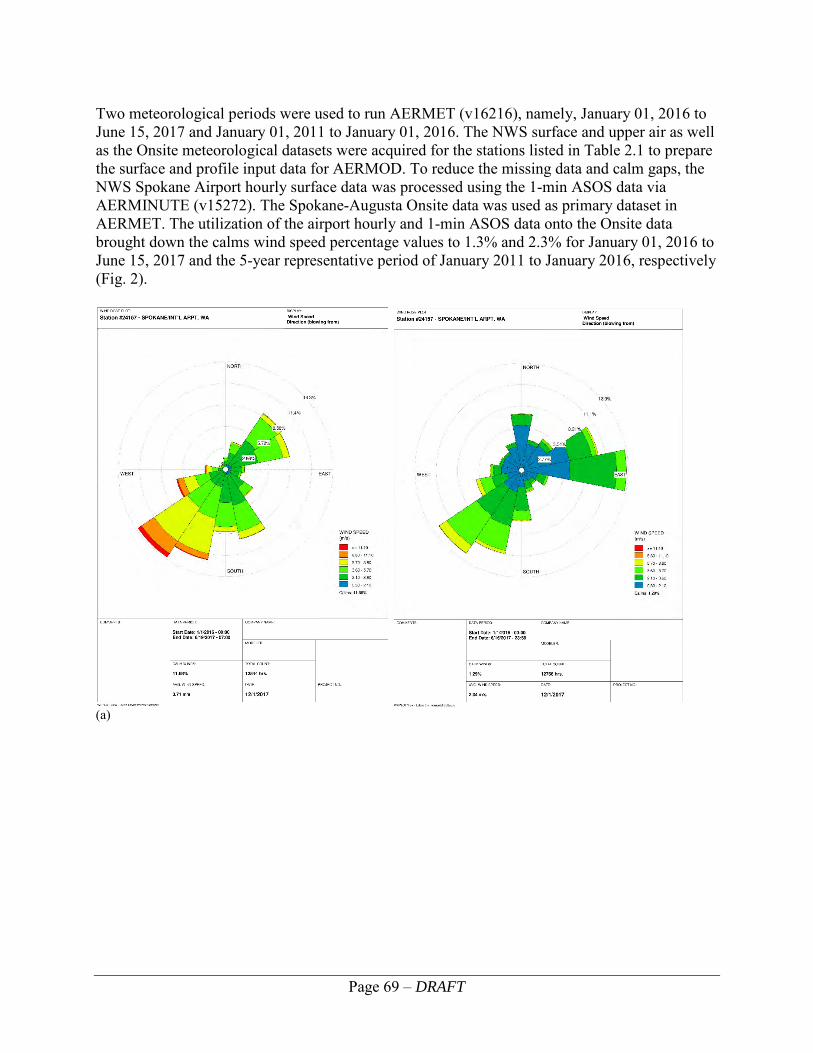
Page 69 – DRAFT

Two meteorological periods were used to run AERMET (v16216), namely, January 01, 2016 to June 15, 2017 and January 01, 2011 to January 01, 2016. The NWS surface and upper air as well as the Onsite meteorological datasets were acquired for the stations listed in Table 2.1 to prepare the surface and profile input data for AERMOD. To reduce the missing data and calm gaps, the NWS Spokane Airport hourly surface data was processed using the 1-min ASOS data via AERMINUTE (v15272). The Spokane-Augusta Onsite data was used as primary dataset in AERMET. The utilization of the airport hourly and 1-min ASOS data onto the Onsite data brought down the calms wind speed percentage values to 1.3% and 2.3% for January 01, 2016 to June 15, 2017 and the 5-year representative period of January 2011 to January 2016, respectively (Fig. 2).

(a)

Page 70 – DRAFT

(b) Fig. 3. Wind Rose plot of raw (left panel) and preprocessed with 1-min ASOS data (right) for (a) January 2016 to June 2017, and (b) January 2011 to January 2016, for Spokane International Airport NWS met station. In addition to the meteorological data prepared to run AERMET, AERSURFACE (v13016) processed the national land cover dataset (NLCD) that was downloaded from the Multi-Resolution Land Characteristics Consortium (MRLC) website to calculate surface characteristics for the Facility. Also obtained from this site is the National Elevation Dataset (NED) for input into AERMAP (v11103) for topographic (elevation) information that is required to run AERMOD. 2.2. Sources There are two flues from the two mass-burn incinerators that release emissions to the atmosphere through a common stack at a height of 171ft. Since the flues have similar physical parameters, the plume dispersion modeling was simulated using a combined ‘one-source’ emission rate. Therefore, parameters are either multiplied by two or an equivalent value is estimated where appropriate. To calculate the emission rates of the different test runs done from 2011 to 2017, the air flow rates and emission factors are taken from each year’s measurement report (see Tables 2.2.1 and 2.2.2).

Page 71 – DRAFT

Table 2.2.1. Spokane WTE Facility air flow data for 2011 thru 2017 test runs taken from Table 2-1(b) of the test run reports of 2011-2017. Bold rows are to indicate PCBs in stack measurements were taken from alternate units each year.

Year Source ID Flue gas

Avg. Temp (F)

Air flow (acfm)

Air flow (dscfm)

Air flow (dscfm)

@7% O2 2017 Unit-1 249.3 120,900 65,200 43,480

Unit-2 258.3 127,700 67,700 45,496 2016 Unit-1 254.4 129,800 70,000 45,000

Unit-2 260.2 129,500 68,400 44,700 2015 Unit-1 260.7 120,000 63,900 43,860

Unit-2 257.1 113,900 61,400 42,979 2014 Unit-1 255.4 119,200 62,900 42,425

Unit-2 252.7 130,200 68,200 46,307 2013 Unit-1 262.1 125,200 66,600 46,969

Unit-2 261.9 122,700 65,400 45,602 2012 Unit-1 266.0 121,500 63,600 44,870

Unit-2 256.4 118,400 62,900 44,438 2011 Unit-1 250.9 133,000 73,900 48,989

Unit-2 255.7 120,500 65,900 44,784 Average Air Flow rate @7% O2 is = 44,252.5dscfm (for both units = 88,505dscfm) Using the emission flow rates and factors in Table 2.2.1 and Table 2.2.2 (see below), emission rates were estimated by assuming the Facility operates at full capacity throughout the year. The concentrations of PCBs in the exhaust flue given in units of mass per dry standard cubic feet of exhaust gas normalized to 7 percent oxygen (ng/dscm @ 7% O2) were taken, after unit adjustment was performed. The concentrations are then multiplied by a flow rate in dry standard cubic feet per minute at 7 percent oxygen (dscfm @7% O2) to develop an emission rate in mass per unit of time using eq. 1. Note that before multiplying by the flow rate, unit conversions or adjustments need to be performed.

𝑄𝑄 [𝜇𝜇𝜇𝜇𝑠𝑠

] = (1000) ∗ � 𝐸𝐸𝑓𝑓𝑓𝑓𝑓𝑓35.3147

� ∗ �𝑈𝑈𝑓𝑓𝑎𝑎𝑎𝑎60� (eq. 1)

Where, Q is the estimated emission rate in units of micrograms per second (µg/s), Efac is the emission factor in units of mass per dry standard cubic feet (ng/dscm) and Uair is the flow rate in dry standard cubic feet per minute (dscfm), both qualities measured at 7% oxygen intake level. In Table 2.2.2, estimated emission rates are given for 2011 – 2017. The 1000 factor is to change the Efac from Nano to Micro scale, while the (1/60) factor is to convert the Uair from a minute to a second time unit. Note that PCBs measure-ments were taken alternately for only one flue each year, as highlighted in bold in Table 2.2.1.

Page 72 – DRAFT

Table 2.2.2. Emission rates estimation for two point sources at 7% O2 (Unit-1 & Unit-2).

Year Pollutant Emission rate – Unit-1 Emission rate – Unit-2 Avg. Run Time (min)

2017 Total PCBs 567.0ng; 179.5ng/dscm 3.854E-06g/s; 3.059E-05lb/hr

263.7

2016 Total PCBs 77.1ng; 25.5ng/dscm 5.416E-07g/s; 4.298E-06lb/hr

259.0

2015 Total PCBs 157.2ng; 55.4ng/dscm; 1.124E-06g/s; 8.92E-06lb/hr

250.0

2014 Total PCBs 1115.4ng;394.0ng/dscm 7.889E-06g/s; 6.261E-05lb/hr

269.3

2013 Total PCBs 361.3ng; 124.2ng/dscm 2.673E-06g/s; 2.121E-05lb/hr

262.0

2012 Total PCBs 120.8ng; 41.8ng/dscm 8.852E-07g/s; 7.025E-06lb/hr

263.0

2011 Total PCBs 365.5ng; 112.1ng/dscm 2.369E-06g/s; 1.880E-5lb/hr

259.3

Measurement runs performed on the flues during the last seven years (2011-2017) showed that PCBs values significantly vary depending on the type of solid wastes burned (Fig. 4). The type of solid wastes burned at the Facility generally categorized as corporate and non-corporate municipality materials. The PCBs emission rate estimates ranged from a maximum of 7.889 µg/s emitted in 2014 to 0.542 µg/s in 2016, with an average amount calculated to be 2.76226 µg/s from each flue.

Fig. 4. Spokane WTE Facility single-unit emission rates estimated from measurement runs for 2011 through 2017 using eq. 1. Table 2.2.3 shows the average stack parameters with emission rates, averaged from measurement runs performed from 2011 – 2017. Note also that the emission rates and actual flow rate need to be added when combining the two unit sources as a single stack for modeling purposes as long as they are under similar other physical parameters and conditions, as shown in Table 2.2.3. The

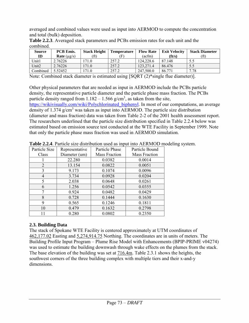
Page 73 – DRAFT

averaged and combined values were used as input into AERMOD to compute the concentration and total (bulk) deposition. Table 2.2.3. Averaged stack parameters and PCBs emission rates for each unit and the combined.

Source ID

PCB Emis. Rate (µg/s)

Stack Height (ft)

Temperature (F)

Flow Rate (acfm)

Exit Velocity (ft/s)

Stack Diameter (ft)

Unit1 2.76226 171.0 257.2 124,228.6 87.148 5.5 Unit2 2.76226 171.0 257.2 123,271.4 86.476 5.5 Combined 5.52452 171.0 257.2 247,500.0 86.771 7.78

Note: Combined stack diameter is estimated using [SQRT (2)*single flue diameter)]. Other physical parameters that are needed as input in AERMOD include the PCBs particle density, the representative particle diameter and the particle phase mass fraction. The PCBs particle density ranged from 1.182 – 1.566 g/cm3, as taken from the site, https://wikivisually.com/wiki/Polychlorinated_biphenyl. In most of our computations, an average density of 1.374 g/cm3 was taken as input into AERMOD. The particle size distribution (diameter and mass fraction) data was taken from Table 2-2 of the 2001 health assessment report. The researchers underlined that the particle size distribution specified in Table 2.2.4 below was estimated based on emission source test conducted at the WTE Facility in September 1999. Note that only the particle phase mass fraction was used in AERMOD simulation. Table 2.2.4. Particle size distribution used as input into AERMOD modeling system.

Particle Size Class

Representative Diameter (um)

Particle Phase Mass Fraction

Particle Bound Mass Fraction

1 22.280 0.0382 0.0014 2 13.154 0.0822 0.0051 3 9.173 0.1074 0.0096 4 3.734 0.0928 0.0204 5 2.038 0.0648 0.0261 6 1.256 0.0542 0.0355 7 0.924 0.0482 0.0429 8 0.728 0.1444 0.1630 9 0.565 0.1246 0.1811 10 0.479 0.1632 0.2798 11 0.280 0.0802 0.2350

2.3. Building Data The stack of Spokane WTE Facility is centered approximately at UTM coordinates of 462,177.02 Easting and 5,274,914.75 Northing. The coordinates are in units of meters. The Building Profile Input Program – Plume Rise Model with Enhancements (BPIP-PRIME v04274) was used to estimate the building downwash through wake effects on the plumes from the stack. The base elevation of the building was set at 716.4m. Table 2.3.1 shows the heights, the southwest corners of the three building complex with multiple tiers and their x-and-y dimensions.

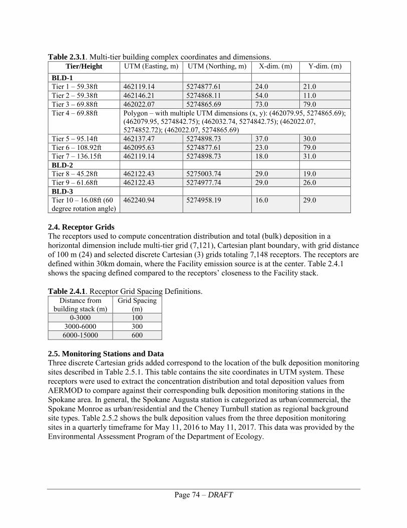
Page 74 – DRAFT

Table 2.3.1. Multi-tier building complex coordinates and dimensions.

Tier/Height UTM (Easting, m) UTM (Northing, m) X-dim. (m) Y-dim. (m) BLD-1 Tier 1 – 59.38ft 462119.14 5274877.61 24.0 21.0 Tier 2 – 59.38ft 462146.21 5274868.11 54.0 11.0 Tier 3 – 69.88ft 462022.07 5274865.69 73.0 79.0 Tier 4 – 69.88ft Polygon – with multiple UTM dimensions (x, y): (462079.95, 5274865.69);

(462079.95, 5274842.75); (462032.74, 5274842.75); (462022.07, 5274852.72); (462022.07, 5274865.69)

Tier 5 – 95.14ft 462137.47 5274898.73 37.0 30.0 Tier 6 – 108.92ft 462095.63 5274877.61 23.0 79.0 Tier 7 – 136.15ft 462119.14 5274898.73 18.0 31.0 BLD-2 Tier 8 – 45.28ft 462122.43 5275003.74 29.0 19.0 Tier 9 – 61.68ft 462122.43 5274977.74 29.0 26.0 BLD-3 Tier 10 – 16.08ft (60 degree rotation angle)

462240.94 5274958.19 16.0 29.0

2.4. Receptor Grids The receptors used to compute concentration distribution and total (bulk) deposition in a horizontal dimension include multi-tier grid (7,121), Cartesian plant boundary, with grid distance of 100 m (24) and selected discrete Cartesian (3) grids totaling 7,148 receptors. The receptors are defined within 30km domain, where the Facility emission source is at the center. Table 2.4.1 shows the spacing defined compared to the receptors’ closeness to the Facility stack. Table 2.4.1. Receptor Grid Spacing Definitions.

Distance from building stack (m)

Grid Spacing (m)

0-3000 100 3000-6000 300 6000-15000 600

2.5. Monitoring Stations and Data Three discrete Cartesian grids added correspond to the location of the bulk deposition monitoring sites described in Table 2.5.1. This table contains the site coordinates in UTM system. These receptors were used to extract the concentration distribution and total deposition values from AERMOD to compare against their corresponding bulk deposition monitoring stations in the Spokane area. In general, the Spokane Augusta station is categorized as urban/commercial, the Spokane Monroe as urban/residential and the Cheney Turnbull station as regional background site types. Table 2.5.2 shows the bulk deposition values from the three deposition monitoring sites in a quarterly timeframe for May 11, 2016 to May 11, 2017. This data was provided by the Environmental Assessment Program of the Department of Ecology.

Page 75 – DRAFT

Table 2.5.1. Three EAP deposition monitoring sites that collected bulk deposition data downwind of the Facility from May 11, 2016 to May 11, 2017.

Site X-UTM (m) Y-UTM (m) Spokane – Augusta 472609.2 5279965.0 Spokane – Monroe 468040.5 5283051.0 Cheney Turnbull 460035.7 5251575.98

Table 2.5.2. Bulk (total) deposition data from EAP monitoring sites averaged per day for three stations for the field measurement run period of four quarters of May 11, 2016 – May 11, 2017.

Monitoring Site Site Type Quarter Start Date End Date Flux (ng/m2 day)

Flux (ng/m2 day) – BC*

Turnbull Regional Background

1 5/11/16 8/10/16 0.37 0.20

2 8/11/16 11/16/16 0.85 0.70 3 11/17/16 2/15/17 2.94 2.83 4 2/16/17 5/11/17 0.06 0.05 Monroe Urban/residential 1 5/11/16 8/10/16 1.24 1.06 2 8/11/16 11/16/16 1.74 1.59 3 11/17/16 2/15/17 3.66 3.55 4 2/16/17 5/11/17 1.38 1.37 Augusta Urban/commercial 1 5/11/16 8/10/16 2.61 2.44 2 8/11/16 11/16/16 10.92 10.78 3 11/17/16 2/15/17 3.71 3.61 4 2/16/17 5/11/17 1.67 1.65

EAP Note: BC = Blank Corrected using equipment blank results.

3. Results The 1-year field study case (Fig. 5a) and 5-year case (Fig. 5b) annual concentration distributions show that highest values were located over the northeastern, south, and west-southwestern region about 2-miles radius from the emission source. This distribution is in agreement with the annual wind flow of the region as depicted in Figs. 3a and 3b wind-rose plots. As can be seen from the figures, the two urban air quality monitoring sites of Augusta and Monroe are outside of the highest concentration impacted areas. In general, the 5-year modeling case shows concentrations over larger area than the 1-year field study case, while the overall concentration distribution trend is similar. Quantitatively, the 5-year modeling results are about 16% higher in concentration and 20% higher in bulk deposition than the 1-year field study period modeling results (Table 3.1). These analyses results highlight the importance of using a longer period of meteorological data to avoid basing decisions on less representative conditions.

Page 76 – DRAFT

(a) (b) Fig. 5. Modeled average annual concentration distribution from the Spokane WTE stack. (a) For May 11, 2016 to May 11, 2017 field measurement case study. (b) Regulatory 5-year modeling study period of January 2011 to December 2015. Coordinates are in UTM (m) and concentration is in picograms per cubic meter (pg = picograms = 10-12 grams). Table 3.1. AERMOD results of concentration and deposition for the 24-hour averaging period for PCBs average particle density and average emission rate at WTE. Modeling

Time Concentration

(pg/m3) Total

Depos. (ng/m2)

Dry Depos. (ng/m2)

Wet Depos. (ng/m2)

1-Yr 2.431 11.056 10.987 6.204 5-Yrs 2.826 13.277 13.273 11.389

The qualitative plots of both the study and the 5-year periods show that total (bulk) deposition across the domain has similar distribution as the concentration, but circumscribed within a smaller area (Figs. 6a & 6b). The modeled deposition over the Spokane urban sites of Augusta and Monroe are very low compared to the observation data at the Monitoring sites. From Figure 6a, the Augusta site is situated within 8 – 10 ng/m2 per year (0.02 – 0.03 ng/m2 per day) of modeled deposition values, while Monroe is within 20 – 50 ng/m2 per year (0.05 – 0.14 ng/m2 per day) deposition. On the other hand, observed bulk deposition values at these two sites vary from 1.2 – 10.9 ng/m2 per day (see Table 3.2). Figure 7 also shows that the logarithmic plot of the modeled PCBs values are less than 2% of the monitored values in four quarters of the study period. In other words, the monitored deposition values are about two orders of magnitude higher than the modeled values. This quantitative and qualitative comparisons show that the PCBs contribution from the Spokane WTE Facility is significantly low. Past AERMOD sensitivity analysis studies suggested that the model generally overestimates observations, especially during calm and/or low wind speeds (e.g., Perry et al. 2005, Duoxing et al. 2007). Therefore the modeling results shown here are likely upper bounds of what the Spokane WTE could contribute to the observed deposition, implying that there must be other contributing PCBs sources in the region.

Page 77 – DRAFT

(a) (b) Fig. 6. Modeled average annual total (bulk) deposition distribution from the Spokane WTE stack. (a) For May 11, 2016 to May 11, 2017 field measurement case study. (b) Regulatory 5-year modeling study period of January 2011 to December 2015. Coordinates are in UTM (m) and deposition is in nanograms per square meter (ng = nanograms = 10-9 grams). Table 3.2. AERMOD modeled and monitored quarterly total (bulk) deposition data for three monitoring sites for the Spokane WTE study period of 05/11/16 to 05/11/17.

Site Site Type Data Type

(ng/m2)

Q1 5/11/16 – 8/10/16

Q2 8/11/16 – 11/16/16

Q3 11/17/16 –

2/15/17

Q4 2/16/17 – 5/11/17

Augusta Commercial Model 0.025 0.023 0.015 0.030 Obs. 2.610 10.920 3.710 1.670

Monroe Residential Model 0.062 0.060 0.041 0.074 Obs. 1.240 1.740 3.660 1.380

Turnbull Regional/ Background

Model 0.004 0.007 0.011 0.004 Obs. 0.370 0.850 2.940 0.060

Page 78 – DRAFT

Fig. 7. Logarithmic plot comparing quarterly bulk deposition of modeled versus monitored data for three sites in pg/m2 per day. (Q1 = 5/11/2017 – 8/10/2016; Q2 = 8/11/2016 – 11/16/2017; Q3 = 11/17/2016 – 2/15/2017; Q4 = 2/16/2017 – 5/11/2017).

4. Summary The Spokane Waste-to-Energy Facility plume dispersion modeling simulation was run for May 11, 2016 to May 11, 2017 and the five-year period of 2011 to 2015. Emission data were collected from reports of the source sampling run tests performed from 2011 to 2017. Other important pollutant and building information were taken from 1991 and 2001 dispersion modeling done for health risk assessment studies. Meteorological data were obtained from the Onsite Spokane Augusta surface, as well as the Spokane International Airport. These meteorological data were most representative for the Facility. AERMOD simulated concentrations and deposition (total, dry and wet) estimates covered a 900 km2 domain, centered on the emission source. Model outputs averaged over 24-hour (8th highest), monthly and the whole period (both 1st highest) averaging time were compared against the 1-year field study period for three monitoring sites. In general, the highest concentration distribution & deposition rates occur within a radius of ~2 mile (3km) from the center of emission source. The main areas susceptible to pollutants from the emission source are the northeastern, south and southwestern regions. The 5-year modeling results are 16% higher in magnitude and cover larger area of concentration distribution when compared to the 1-year field study period. However, the overall concertation distribution trend and orientation are similar. These results highlight the importance of using a longer representative modeling period to better inform decision making. Bulk deposition data from three monitoring sites of Spokane- Augusta, Spokane- Monroe and Cheney-Turnbull were also compared against their corresponding model results for the study period. The WTE’s PCB emissions account for about 2% of the measured deposition at these sites. As AERMOD modeling tends to overestimate observed values, this study suggests the presence of other contributing PCB sources to these sites.

Page 79 – DRAFT

5. Reference

Agency for Toxic Substances and Disease Registry, Last updated Aug. 9, 2016. Polychlorinated Biphenyls (PCBs) Toxicity, What Standards and Regulations Exist for PCB Exposure? www.atsdr.cdc.gov/csem/csem.asp?csem=30&po=8.

Environmental Toxicology International, Inc. Seattle, WA, 1991. Spokane Regional Solid Waste Disposal Project Dispersion Modeling Analysis. Preparer address: ‘21907 64th Ave, W Suite 230, Mountlake Terrace, WA 98043.’

Duoxing, Yang, C. Gangcai, and Y. Yunjiang, 2007. Inter-comparison of AERMOD and ISC3 modeling results to the Alaska tracer field experiment. Chinese J. Geochem., 26, 182-185.

Perry, Steven G., A. J. Cimorelli, R. J. Paine, R. W. Brode, J. C. Weil, A. Venkatram, R. B. Wilson, R. F. Lee, and W. D. Peters, 2005. AERMOD: A dispersion model for industrial source applications. Part II: Model performance against 17 field study databases. J. Appl. Meteor., 44, 694-708.

Pioneer Technologies Corporation, Olympia, WA, 2001. Spokane Waste-To-Energy Facility Human Health Risk Assessment. Preparer address: ‘2612 Yelm Hwy SE, Suite B Olympia, WA 98501-4826; www.uspioneer.com.’

Stationary source sampling report, Spokane Waste to Energy, Spokane, WA, 2011-2017. Preparer address: ‘DEECO Inc., 3404 Lake Woodard Rd, Raleigh, NC 27604; www.stacksampling.com.’

Wikivisually. Polychlorinated Biphenyl (PCB) wikivisually.com/wiki/Polychlorinated_biphenyl. Acronyms

AERMOD AMS/EPA Regulatory Model AERMET Meteorological pre-processor for AERMOD AERMAP Terrain pre-processor for AERMOD AERMINUTE 1-min ASOS wind data averaging processor for AERMET/AERMOD AERSURFACE Surface characteristics pre-processor for AERMOD AMS American Meteorological Society ASOS Automated Surface Observing System BPIP-PRIME Building Profile Input Program – Plume Rise Model with Enhancements EAP Environmental Assessment Program, Department of Ecology EPA U.S. Environmental Protection Agency NWS National Weather Service PCBs Polychlorinated Biphenyls TPD Tons per day WTE Waste to Energy

Page 80 – DRAFT

Appendix E. Glossary, Acronyms, and Abbreviations Glossary Airshed: A geographical area within which the air frequently is confined or channeled, with all parts of the area thus being subject to similar conditions of air pollution.

Clean Water Act: A federal act passed in 1972 that contains provisions to restore and maintain the quality of the nation’s waters. Section 303(d) of the Clean Water Act establishes the TMDL program.

Flux: An amount of a substance deposited in a given area per a period of time. An example for atmospheric deposition flux is ng/m2-per day.

PCB congener: Any single, unique, well-defined chemical compound in the PCB group. They are identified by the number and position of chlorine atoms around the biphenyl rings. There are theoretically 209 possible congeners.

Stormwater: The portion of precipitation that does not naturally percolate into the ground or evaporate but instead runs off roads, pavement, and roofs during rainfall or snow melt. Stormwater can also come from hard or saturated grass surfaces such as lawns, pastures, playfields, and from gravel roads and parking lots.

Total Maximum Daily Load (TMDL): Water cleanup plan. A distribution of a substance in a waterbody designed to protect it from not meeting (exceeding) water quality standards. A TMDL is equal to the sum of all of the following: (1) individual wasteload allocations for point sources, (2) the load allocations for nonpoint sources, (3) the contribution of natural sources, and (4) a Margin of Safety to allow for uncertainty in the wasteload determination. A reserve for future growth is also generally provided.

Watershed: A drainage area or basin in which all land and water areas drain or flow toward a central collector such as a stream, river, or lake at a lower elevation.

303(d) list: Section 303(d) of the federal Clean Water Act requires Washington State to periodically prepare a list of all surface waters in the state for which beneficial uses of the water – such as for drinking, recreation, aquatic habitat, and industrial use – are impaired by pollutants. These are water quality-limited estuaries, lakes, and streams that fall short of state surface water quality standards and are not expected to improve within the next two years.

Acronyms and Abbreviations

AQP Ecology’s Air Quality Program Ecology Washington State Department of Ecology EAP Ecology’s Environmental Assessment Program EIM Environmental Information Management database EPA U.S. Environmental Protection Agency

Page 81 – DRAFT

MEL Manchester Environmental Laboratory QAPP Quality Assurance Project Plan QA Quality assurance QC Quality control PCA Principle Component Analysis PM2.5 Particulate matter size 2.5 microns and smaller PM10 Particulate matter size 10 microns and smaller PUF Polyurethane foam – a type of sorption media RPD Relative percent difference SOP Standard operating procedures SRCAA Spokane Regional Clean Air Agency SRRTTF Spokane River Regional Toxics Taskforce TMDL (See Glossary above) tPCB Total PCB XAD-2 A type of sorption media made up of small polymer resin beads Units of Measurement °C degrees centigrade cm centimeter °F degrees farenheight km kilometer, a unit of length equal to 1,000 meters km2 square kilometer L liter m3 meter cubed m3/min. meter cubed per minute mL milliliters ng/L nanograms per liter (parts per trillion) ng/m2-day nanogram per meter squared per day pg/m3 picogram per meter cubed pg/L picograms per liter (parts per quadrillion) ug/m3 microgram per meter cubed