spring 2006parallel processing, low-diameter architecturesslide 1 part iv low-diameter architectures

Spring 2006 Parallel Processing, Low-Diameter Architectures Slide 1

Part IVLow-Diameter Architectures


About This Presentation

Edition Released Revised Revised

First Spring 2005 Spring 2006

This presentation is intended to support the use of the textbook Introduction to Parallel Processing: Algorithms and Architectures (Plenum Press, 1999, ISBN 0-306-45970-1). It was prepared by the author in connection with teaching the graduate-level course ECE 254B: Advanced Computer Architecture: Parallel Processing, at the University of California, Santa Barbara. Instructors can use these slides in classroom teaching and for other educational purposes. Any other use is strictly prohibited. © Behrooz Parhami


IV Low-Diameter Architectures

Study the hypercube and related interconnection schemes:• Prime example of low-diameter (logarithmic) networks• Theoretical properties, realizability, and scalability• Complete our view of the “sea of interconnection nets”

Topics in This Part

Chapter 13 Hypercubes and Their Algorithms

Chapter 14 Sorting and Routing on Hypercubes

Chapter 15 Other Hypercubic Architectures

Chapter 16 A Sampler of Other Networks


13 Hypercubes and Their Algorithms

Study the hypercube and its topological/algorithmic properties:• Develop simple hypercube algorithms (more in Ch. 14)• Learn about embeddings and their usefulness

Topics in This Chapter

13.1 Definition and Main Properties

13.2 Embeddings and Their Usefulness

13.3 Embedding of Arrays and Trees

13.4 A Few Simple Algorithms

13.5 Matrix Multiplication

13.6 Inverting a Lower-Triangular Matrix


13.1 Definition and Main Properties

P 1

P 2

P 3

P 4

P 5

P 6

P 7

P 8

P 0

P P P

P P P

P P P

0

1

2

3

4

5

6

7

8

Intermediate architectures: logarithmic or sublogarithmic

diameter

Begin studying networks that are intermediate between diameter-1 complete network and diameter-p1/2 mesh

Complete network

n/2 log n log n / log log n n 1 1 n 2

Sublogarithmic diameter Superlogarithmic diameter

PDN Star, pancake

Binary tree, hypercube

Torus Ring Linear array


Hypercube and Its HistoryBinary tree has logarithmic diameter, but small bisectionHypercube has a much larger bisectionHypercube is a mesh with the maximum possible number of dimensions

2 2 2 . . . 2 q = log2 p

We saw that increasing the number of dimensions made it harder to design and visualize algorithms for the meshOddly, at the extreme of log2 p dimensions, things become simple again!

Brief history of the hypercube (binary q-cube) architecture Concept developed: early 1960s [Squi63] Direct (single-stage) and indirect (multistage) versions: mid 1970s Initial proposals [Peas77], [Sull77] included no hardware Caltech’s 64-node Cosmic Cube: early 1980s [Seit85] Introduced an elegant solution to routing (wormhole switching)Several commercial machines: mid to late 1980s Intel PSC (personal supercomputer), CM-2, nCUBE (Section 22.3)


Basic Definitions

Hypercube is generic term; 3-cube, 4-cube, . . . , q-cube in specific cases

0 1 00 01

10 11

(a) Binary 1-cube, built of two binary 0-cubes, labeled 0 and 1

(b) Binary 2-cube, built of two binary 1-cubes, labeled 0 and 1

0

1

(c) Binary 3-cube, built of two binary 2-cubes, labeled 0 and 1

0

000 001

010 011

100 101

110 111

1

000

001

010

011

100

101

110

111

(d) Binary 4-cube, built of two binary 3-cubes, labeled 0 and 1

0 1

0000

0001

0010

0011

0100

0101

0110

0111

1000

1001

1010

1011

1100

1101

1110

1111

Fig. 13.1 The recursive structure of binary hypercubes.

Parameters:

p = 2q

B = p/2 = 2q–1

D = q = log2p

d = q = log2p


Only sample wraparound links are shown to avoid clutter

The 64-Node Hypercube

Isomorphic to the 4 4 4 3D torus (each has 64 6/2 links)


Neighbors of a Node in a Hypercube

xq–1xq–2 . . . x2x1x0 ID of node x

xq–1xq–2 . . . x2x1x0 dimension-0 neighbor; N0(x) xq–1xq–2 . . . x2x1x0 dimension-1 neighbor; N1(x) . . . . . .xq–1xq–2 . . . x2x1x0 dimension-(q – 1) neighbor; Nq–1(x)

The q neighbors of node x

Nodes whose labels differ in k bits (at Hamming distance k) connected by shortest path of length k

Both node- and edge-symmetric

Strengths: symmetry, log diameter, and linear bisection width

Weakness: poor scalability

Dim 0

Dim 1

Dim 2 Dim 3

0100 0101

0110

00001100

1101

1111

0111

0011

x

1011

0010

1010

x


13.2 Embeddings and Their Usefulness

Fig. 13.2 Embedding a seven-node binary tree into 2D meshes of various sizes.

0

2

4 3

1

6 5

0 2

4 3

1 6

5

0,1

2

4

3

6

5

6

0 1

3,4

2,5

a b

c d e f

a b

c

d

e

f

a b

c

d

e

f

b

f c, d

Dilation = 1Congestion = 1Load factor = 1



Dilation: Longest path onto which an edge is mapped (routing slowdown)Congestion: Max number of edges mapped onto one edge (contention slowdown)Load factor: Max number of nodes mapped onto one node (processing slowdown)

Expansion: ratio of the number of nodes (9/7, 8/7, and 4/7 here)


13.3 Embedding of Arrays and Trees

Alternate inductive proof: Hamiltonicity of the q-cube is equivalent to the existence of a q-bit Gray code

Fig. 13.3 Hamiltonian cycle in the q-cube.

(q – 1)-cube 0

x

(q – 1)-cube 1

N (x)k

N (x)q–1

N (N (x)) q–1 k

(q – 1)-bit Gray code

000 . . . 000000 . . . 001000 . . . 011 . . .100 . . . 000

000

01

111

100 . . . 000 . . .000 . . . 011000 . . . 010000 . . . 000

(q – 1)-bit Gray codein reverse

Basis: q-bit Gray code beginning with the all-0s codeword and ending with 10q–1 exists for q = 2: 00, 01, 11, 10


Mesh/Torus Embedding in a Hypercube

Is a mesh or torus a subgraph of the hypercube of the same size?

Dim 0

Dim 1

Dim 2 Dim 3

Column 0

Column 1

Column 2

Column 3

Fig. 13.5 The 4 4 mesh/torus is a subgraph of the 4-cube.

We prove this to be the case for a torus (and thus for a mesh)


Torus is a Subgraph of Same-Size Hypercube

A tool used in our proof

Product graph G1 G2:

Has n1 n2 nodes

Each node is labeled by a pair of labels, one from each component graph

Two nodes are connected if either component of the two nodes were connected in the component graphs

Fig. 13.4 Examples of product graphs.

The 2a 2b 2c . . . torus is the product of 2a-, 2b-, 2c-, . . . node ringsThe (a + b + c + ... )-cube is the product of a-cube, b-cube, c-cube, . . .The 2q-node ring is a subgraph of the q-cubeIf a set of component graphs are subgraphs of another set, the product graphs will have the same relationship

=3-by-2 torus

=

=

0

1

2

a

b

0a

1a

2a0b

1b

2b


Embedding Trees in the Hypercube

The (2q – 1)-node complete binary tree is not a subgraph of the q-cube

even weight

odd weightseven weights

odd weights

even weights

Proof by contradiction based on the parity of node label weights (number of 1s is the labels)

The 2q-node double-rooted complete binary tree is a subgraph of the q-cube

Fig. 13.6 The 2q-node double-rooted complete binary tree is a subgraph of the q-cube.

New Roots

x N (N (x)) N (N (x))

2 -node double-rooted complete binary tree

q Double-rooted tree in the (q–1)-cube 0

Double-rooted tree in the (q–1)-cube 1

N (x)c

N (x)b

N (x)a

b c

bc

N (N (x)) N (N (x))

c a

ca


A Useful Tree Embedding in the Hypercube

The (2q – 1)-node complete binary tree can be embedded into the (q – 1)-cube

Fig. 13.7 Embedding a 15-node complete binary tree into the 3-cube.

Processor 000

001

010

011

100

101

110

111

Dim-2 link

Dim-1 links

Dim-0 links

Despite the load factor of q, many tree algorithms entail no slowdown


13.4 A Few Simple Algorithms

Fig. 13.8 Semigroup computation on a 3-cube.

Semigroup computation on the q-cubeProcessor x, 0 x < p do t[x] := v[x] {initialize “total” to own value}for k = 0 to q – 1 processor x, 0 x < p, do get y :=t[Nk(x)] set t[x] := t[x] yendfor

0

2

1

3

4

6

5

7

0-1

2-3

0-1

2-3

4-5

6-7

4-5

6-7

0-3

0-3

0-3

0-3

4-7

4-7

4-7

4-7

0-7

0-7

0-7

0-7

0-7

0-7

0-7

0-7

Commutativity of the operator is implicit here.

How can we remove this assumption?


Parallel Prefix Computation

Fig. 13.8 Semigroup computation on a 3-cube.

Commutativity of the operator is implicit in this algorithm as well.

How can we remove this assumption?

t : subcube “total”

u : subcube prefix0

2

1

3

4

6

5

7

0-1

2-3

0-1

2-3

4-5

6-7

4-5

6-7

0-3

0-3

0-3

0-3

4-7

4-7

4-7

4-7

4 4-5

0 0-1

6 6-7

2 2-3

t: Subcube "total"u: Subcube prefix

4

0

0-2

4-6

0-1

0-3

4-5

4-7

0-4

0 0-1

0-2

0-5

0-6 0-7

0-3

All "totals" 0-7

Legend t

u

Parallel prefix computation on the q-cubeProcessor x, 0 x < p, do t[x] := u[x] := v[x] {initialize subcube “total” and partial prefix}for k = 0 to q – 1 processor x, 0 x < p, do get y :=t[Nk(x)] set t[x] := t[x] y if x > Nk(x) then set u[x] := y u[x]endfor


Sequence Reversal on the Hypercube

Fig. 13.11 Sequence reversal on a 3-cube.

Reversing a sequence on the q-cubefor k = 0 to q – 1 Processor x, 0 x < p, do get y := v[Nk(x)] set v[x] := yendfor

000

001

010

011

100

101

110

111

000

001

010

011

101

110

111

000

001

010

011

100

101

110

111

000

001

010

011

100

101

110

111

100 a b

c d

e f

g h

a b

c d

e f

g h

g h

e f

c d

a b

c d

a b

g h

e f


Ascend, Descend, and Normal Algorithms

Graphical depiction of ascend, descend, and normal algorithms.

Hypercube Dimension

q–1

3 2 1 0

Algorithm Steps0 1 2 3 . . .

.

.

.

Ascend

Descend

Normal

0

2

1

3

4

6

5

7

0-1

2-3

0-1

2-3

4-5

6-7

4-5

6-7

0-3

0-3

0-3

0-3

4-7

4-7

4-7

4-7

4 4-5

0 0-1

6 6-7

2 2-3

t: Subcube "total"u: Subcube prefix

4

0

0-2

4-6

0-1

0-3

4-5

4-7

0-4

0 0-1

0-2

0-5

0-6 0-7

0-3

All "totals" 0-7

Legend t

u Parallel prefix

000

001

010

011

100

101

110

111

000

001

010

011

101

110

111

000

001

010

011

100

101

110

111

000

001

010

011

100

101

110

111

100 a b

c d

e f

g h

a b

c d

e f

g h

g h

e f

c d

a b

c d

a b

g h

e f

Sequence reversal

Semigroup

0

2

1

3

4

6

5

7

0-1

2-3

0-1

2-3

4-5

6-7

4-5

6-7

0-3

0-3

0-3

0-3

4-7

4-7

4-7

4-7

0-7

0-7

0-7

0-7

0-7

0-7

0-7

0-7

Dimension-order communication


13.5 Matrix Multiplication

Fig. 13.12 Multiplying two 2 2 matrices on a 3-cube.

0

2

1

3

4

6

5

7

1 5

2 6

3 7

4 8

1 2 3 4

5 6 7 8

000 001

010 011

100 101

110 111

1 5

2 6

3 7

4 8

1 5

2 6

3 7

4 8

1 5

1 6

3 7

3 8

2 5

2 6

4 7

4 8

1 5

1 6

3 5

3 6

2 7

2 8

4 7

4 8

14 16

5

15

28

6

32

18

19 22

43 50

RR

AB

RR

AB

RC

RR

AB

RR

AB

R := R RC A B

1. Place elements of A and B in registers RA & RB of m2 processors with the IDs 0jk

p = m3 = 2q processors, indexed as ijk (with three q/3-bit segments)

2. Replicate inputs: communicate across 1/3 of the dimensions

3, 4. Rearrange the data by communicating across the remaining 2/3 of dimensions so that processor ijk has Aji and Bik

6. Move Cjk to processor 0jk


Analysis of Matrix Multiplication

The algorithm involves communication steps in three loops, each with q / 3 iterations (in one of the 4 loops, 2 values are exchanged per iteration)

Tmul (m, m3) =

O(q) = O(log m)

0

2

1

3

4

6

5

7

1 5

2 6

3 7

4 8

1 2 3 4

5 6 7 8

000 001

010 011

100 101

110 111

1 5

2 6

3 7

4 8

1 5

2 6

3 7

4 8

1 5

1 6

3 7

3 8

2 5

2 6

4 7

4 8

1 5

1 6

3 5

3 6

2 7

2 8

4 7

4 8

14 16

5

15

28

6

32

18

19 22

43 50

RR

AB

RR

AB

RC

RR

AB

RR

AB

R := R RC A B

Analysis in the case of block matrix multiplication (m m matrices):Matrices are partitioned into p1/3 p1/3 blocks of size (m / p1/3) (m / p1/3) Each communication step deals with m2 / p2/3 block elements Each multiplication entails 2m3/p arithmetic operations

Tmul(m, p) = m2 / p2/3 O(log p) + 2m3 / p Communication Computation


13.6 Inverting a Lower-Triangular Matrix

Tinv(m) = Tinv(m/2) + 2Tmul(m/2) = Tinv(m/2) + O(log m) = O(log2m)

B 0 B–1 0For A = we have A–1 =

C D –D–1CB–1 D–1

0

0 a ij

a ij

i j

i j

Because B and D are both lower triangular, the same algorithm can be used recursively to invert them in parallel

B 0 B–1 0 BB–1 0 = C D –D–1CB–1 D–1 CB–1 – DD–1CB–1 DD–1

I

I0


14 Sorting and Routing on Hypercubes

Study routing and data movement problems on hypercubes:• Learn about limitations of oblivious routing algorithms• Show that bitonic sorting is a good match to hypercube


14.1 Defining the Sorting Problem

14.2 Bitonic Sorting on a Hypercube

14.3 Routing Problems on a Hypercube

14.4 Dimension-Order Routing

14.5 Broadcasting on a Hypercube

14.6 Adaptive and Fault-Tolerant Routing


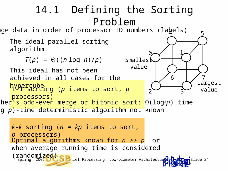
14.1 Defining the Sorting ProblemArrange data in order of processor ID numbers (labels)

1-1 sorting (p items to sort, p processors)

k-k sorting (n = kp items to sort, p processors)

0

2

1

3

4

6

5

7

The ideal parallel sorting algorithm:

T(p) = ((n log n)/p)

This ideal has not been achieved in all cases for the hypercube

Smallestvalue

Largestvalue

Batcher’s odd-even merge or bitonic sort: O(log2p) timeO(log p)-time deterministic algorithm not known

Optimal algorithms known for n >> p or when average running time is considered (randomized)


Hypercube Sorting: Attempts and Progress

No bull’s eye yet!

There are three categories of practical sorting algorithms:

1. Deterministic 1-1, O(log2p)-time

2. Deterministic k-k, optimal for n >> p (that is, for large k)

3. Probabilistic (1-1 or k-k)

Pursuit of O(log p)-time algorithm is of theoretical interest only

? log n

One of the oldest parallel algorithms; discovered 1960, published 1968

Practical, deterministic

Fewer than p items

Practical, probabilistic

More than p items

1960s

1990

1988

1987

1980

log n log log n

log n (log log n) 2

(n log n)/p for n >> p

log n randomized

log p log n/log(p/n), n p/4; 1–

log n for n = p, bitonic 2

in particular, log p for n = p


Bitonic Sequences

Bitonic sequence:

1 3 3 4 6 6 6 2 2 1 0 0 Rises, then falls

8 7 7 6 6 6 5 4 6 8 8 9 Falls, then rises

8 9 8 7 7 6 6 6 5 4 6 8 The previous sequence, right-rotated by 2

(a)

(b)

Cyclic shift of (a)

Cyclic shift of (b)

Fig. 14.1 Examples of bitonic sequences.

In Chapter 7, we designed bitonic sorting nets

Bitonic sorting is ideally suited to hypercube


Sorting a Bitonic Sequence on a Linear Array

Fig. 14.2 Sorting a bitonic sequence on a linear array.

Bitonic sequence Shifted right half

Shift right half of data to left half (superimpose the two halves)

In each position, keep the smaller of the two values and ship the larger value to the right

Each half is a bitonic sequence that can be sorted independently

0 1 2 n 1

0 1 2 n 1

n/2

n/2

Time needed to sort a bitonic sequence on a p-processor linear array:

B(p) = p + p/2 + p/4 + . . . + 2 = 2p – 2

Not competitive, because we can sort an arbitrary sequence in 2p – 2 unidirectional communication steps using odd-even transposition


Bitonic Sorting on a Linear Array

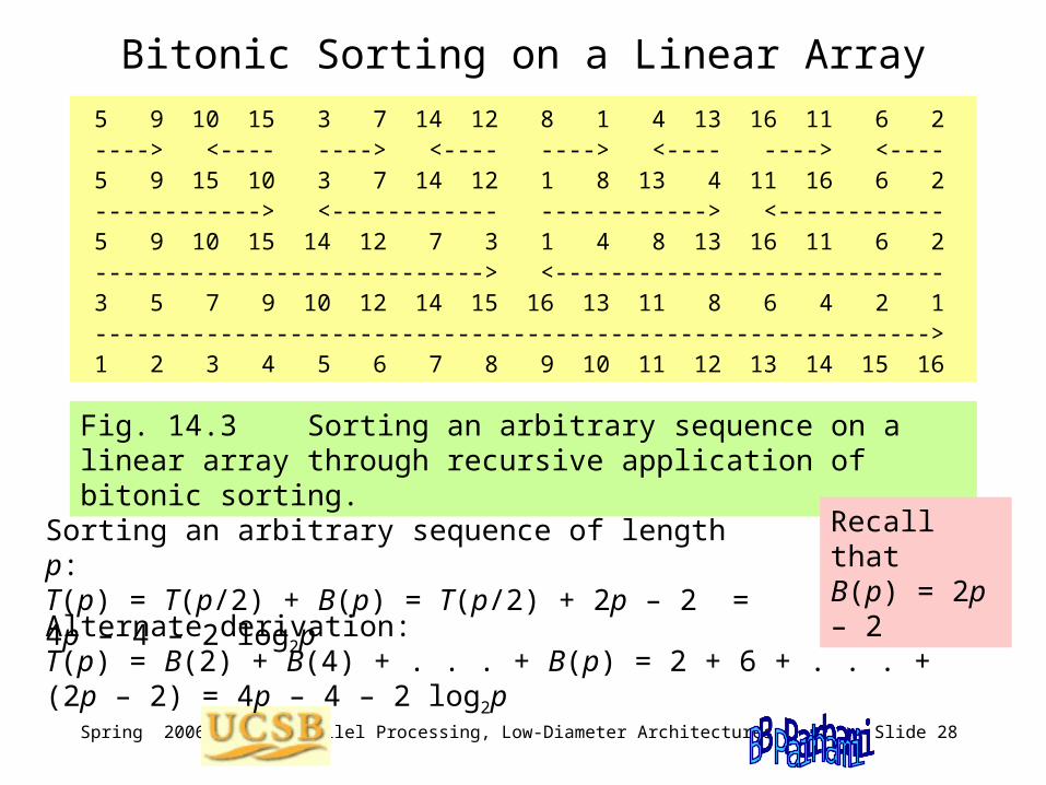
5 9 10 15 3 7 14 12 8 1 4 13 16 11 6 2 ----> <---- ----> <---- ----> <---- ----> <---- 5 9 15 10 3 7 14 12 1 8 13 4 11 16 6 2 ------------> <------------ ------------> <------------ 5 9 10 15 14 12 7 3 1 4 8 13 16 11 6 2 ----------------------------> <---------------------------- 3 5 7 9 10 12 14 15 16 13 11 8 6 4 2 1 ------------------------------------------------------------> 1 2 3 4 5 6 7 8 9 10 11 12 13 14 15 16

Fig. 14.3 Sorting an arbitrary sequence on a linear array through recursive application of bitonic sorting.

Recall that B(p) = 2p – 2

Sorting an arbitrary sequence of length p:T(p) = T(p/2) + B(p) = T(p/2) + 2p – 2 = 4p – 4 – 2 log2p

Alternate derivation:T(p) = B(2) + B(4) + . . . + B(p) = 2 + 6 + . . . + (2p – 2) = 4p – 4 – 2 log2p


For linear array, the 4p-step bitonic sorting algorithm is inferior to odd-even transposition which requires p compare-exchange steps (or 2p unidirectional communications)

The situation is quite different for a hypercube

14.2 Bitonic Sorting on a Hypercube

Sorting a bitonic sequence on a hypercube: Compare-exchange values in the upper subcube (nodes with xq–1 = 1) with those in the lower subcube (xq–1 = 0); sort the resulting bitonic half-sequences

B(q) = B(q – 1) + 1 = q

Sorting a bitonic sequence of size n on q-cube, q = log2nfor l = q – 1 downto 0 processor x, 0 x < p, do if xl = 0 then get y := v[Nl(x)]; keep min(v(x), y); send max(v(x), y) to Nl(x) endifendfor

Complexity: 2q communication steps

This is a “descend” algorithm


Bitonic Sorting on a Hypercube

T(q) = T(q – 1) + B(q)

= T(q – 1) + q = q(q + 1)/2 = O(log2 p)

000

001

010

011

100

101

110

111

000

001

010

011

101

110

111

000

001

010

011

100

101

110

111

000

001

010

011

100

101

110

111

100 b a

c c

f e

h g

a c

e g

h f

c b

c a

b c

f h

g e

b a

c c

f e

g h

Data ordering in lower cube

Data ordering in upper cube

Dimension 2 Dimension 1 Dimension 0

Fig. 14.4 Sorting a bitonic sequence of size 8 on the 3-cube.


14.3 Routing Problems on a HypercubeRecall the following categories of routing algorithms:

Off-line: Routes precomputed, stored in tablesOn-line: Routing decisions made on the fly

Oblivious: Path depends only on source and destinationAdaptive: Path may vary by link and node conditions

Good news for routing on a hypercube:Any 1-1 routing problem with p or fewer packets can be solved in O(log p) steps, using an off-line algorithm; this is a consequence of there being many paths to choose from

Bad news for routing on a hypercube:Oblivious routing requires (p1/2/log p) time in the worst case (only slightly better than mesh)In practice, actual routing performance is usually much closer to the log-time best case than to the worst case.


Limitations of Oblivious Routing

Theorem 14.1: Let G = (V, E) be a p-node, degree-d network. Any oblivious routing algorithm for routing p packets in G needs (p1/2/d) worst-case time

Proof Sketch: Let Pu,v be the unique path used for routing messages from u to v

There are p(p – 1) possible paths for routing among all node pairs

These paths are predetermined and do not depend on traffic within the network

Our strategy: find k node pairs ui, vi (1 i k) such that ui uj and vi vj for i j, and Pui,vi

all pass through the same edge e

Because 2 packets can go through a link in one step, (k) steps will be needed for some 1-1 routing problem

The main part of the proof consists of showing that k can be as large as p1/2/d

v


14.4 Dimension-Order Routing Source 01011011 Destination 11010110 Differences ^ ^^ ^ Path: 01011011

1101101111010011 1101011111010110

dim 0 dim 1 dim 2

0 1 2 3

q + 1 Columns

0 1 2 3 4 5 6 7

0 1 2 3 4 5 6 7

2 Rowsq

0 1 2 3 4 5 6 7

Hypercube

Unfold

Fold

Fig. 14.5 Unfolded 3-cube or the 32-node butterfly network.

Unfolded hypercube (indirect cube, butterfly) facilitates the discussion, visualization, and analysis of routing algorithms

Dimension-order routing between nodes i and j in q-cube can be viewed as routing from node i in column 0 (q) to node j in column q (0) of the butterfly


Self-Routing on a Butterfly Network

From node 3 to 6: routing tag = 011 110 = 101 “cross-straight-cross”From node 3 to 5: routing tag = 011 101 = 110 “cross-cross-straight”From node 6 to 1: routing tag = 110 001 = 111 “cross-cross-cross”

dim 0 dim 1 dim 2

0 1 2 3

0 1 2 3 4 5 6 7

0 1 2 3 4 5 6 7

Ascend Descend

Fig. 14.6 Example dimension-order routing paths.

Number of cross links taken = length of path in hypercube


Butterfly Is Not a Permutation Networkdim 0 dim 1 dim 2

0 1 2 3

A B C D

A B C D

0 1 2 3 4 5 6 7

0 1 2 3 4 5 6 7

Fig. 14.7 Packing is a “good” routing problem for dimension-order routing on the hypercube.

dim 0 dim 1 dim 2

0 1 2 3

0 1 2 3 4 5 6 7

0 1 2 3 4 5 6 7

Fig. 14.8 Bit-reversal permutation is a “bad” routing problem for dimension-order routing on the hypercube.


Why Bit-Reversal Routing Leads to Conflicts?

Consider the (2a + 1)-cube and messages that must go from nodes 0 0 0 . . . 0 x1 x2 . . . xa–1 xa to nodes xa xa–1 . . . x2 x1 0 0 0 . . . 0

a + 1 zeros a + 1 zeros

If we route messages in dimension order, starting from the right end, all of these 2a = (p1/2) messages will pass through node 0

Consequences of this result:

1. The (p1/2) delay is even worse than (p1/2/d) of Theorem 14.1

2. Besides delay, large buffers are needed within the nodes

True or false? If we limit nodes to a constant number of message buffers, then the (p1/2) bound still holds, except that messages are queued at several levels before reaching node 0

Bad news (false): The delay can be (p) for some permutations

Good news: Performance usually much better; i.e., log2 p + o(log p)


Wormhole Routing on a Hypercube

dim 0 dim 1 dim 2

0 1 2 3

A B C D

A B C D

0 1 2 3 4 5 6 7

0 1 2 3 4 5 6 7

dim 0 dim 1 dim 2

0 1 2 3

0 1 2 3 4 5 6 7

0 1 2 3 4 5 6 7

Good/bad routing problems are good/bad for wormhole routing as well

Dimension-order routing is deadlock-free


14.5 Broadcasting on a Hypercube

Flooding: applicable to any network with all-port communication

00000 Source node

00001, 00010, 00100, 01000, 10000 Neighbors of source

00011, 00101, 01001, 10001, 00110, 01010, 10010, 01100, 10100, 11000 Distance-2 nodes

00111, 01011, 10011, 01101, 10101, 11001, 01110, 10110, 11010, 11100 Distance-3 nodes

01111, 10111, 11011, 11101, 11110 Distance-4 nodes

11111 Distance-5 node

Binomial broadcast tree with single-port communication

0 1 2 3 4 5

Time00000

10000

01000 11000

00100 01100 10100 11100

00001

00010

Fig. 14.9 The binomial broadcast tree for a 5-cube.


Hypercube Broadcasting Algorithms

Fig. 14.10 Three hypercube broadcasting schemes as performed on a 4-cube.

Binomial-t ree scheme (nonpipelined)

Pipelined binomial-tree scheme

Johnsson & Ho’s method

ABCD

ABCD

ABCD ABCD

A

A

A

B

B

B

C

A

A

A

A

C

C

D

B

B

B

B

A

A

A

A

A

A

A A

A

A

A

A

A

A

A

A

A

A

A

A

A

A A

To avoid clutter, only A shown

B

B

B

B

B

B

B

B

B

B B C C

C C

C

C D

D

D

D

D

D

D

C


14.6 Adaptive and Fault-Tolerant Routing

There are up to q node-disjoint and edge-disjoint shortest paths between any node pairs in a q-cube

Thus, one can route messages around congested or failed nodes/links

A useful notion for designing adaptive wormhole routing algorithms is that of virtual communication networks

Each of the two subnetworks in Fig. 14.11 is acyclic

Hence, any routing scheme that begins by using links in subnet 0, at some point switches the path to subnet 1, and from then on remains in subnet 1, is deadlock-free

0

2

1

3

4

6

5

7

0

2

1

3

4

6

5

7

Subnetwork 0 Subnetwork 1

Fig. 14.11 Partitioning a 3-cube into subnetworks for deadlock-free routing.


The fault diameter of the q-cube is q + 1.

Robustness of the Hypercube

Source

Destination

X

X

X

Three faulty nodes

The node that is furthest from S is not its diametrically opposite node in the fault-free hypercube

SRich connectivity provides many alternate paths for message routing


15 Other Hypercubic Architectures

Learn how the hypercube can be generalized or extended:• Develop algorithms for our derived architectures• Compare these architectures based on various criteria


15.1 Modified and Generalized Hypercubes

15.2 Butterfly and Permutation Networks

15.3 Plus-or-Minus-2i Network

15.4 The Cube-Connected Cycles Network

15.5 Shuffle and Shuffle-Exchange Networks

15.6 That’s Not All, Folks!


15.1 Modified and Generalized Hypercubes

Fig. 15.1 Deriving a twisted 3-cube by redirecting two links in a 4-cycle.

Twisted 3-cube

0

2

1

3

4

6

5

7

5

3-cube and a 4-cycle in it

0

2

1

3

4

6 7

Diameter is one less than the original hypercube


Folded Hypercubes

Fig. 15.2 Deriving a folded 3-cube by adding four diametral links.

Folded 3-cube

0

2

1

3

4

6

5

7

5

A diametral path in the 3-cube

0

2

1

3

4

6 7

Fig. 15.3 Folded 3-cube viewed as 3-cube with a redundant dimension.

Rotate 180 degrees

Folded 3-cube with Dim-0 links removed

0

2

7

5

4

6

3

1

5

0

2

1

3

4

6 7

After renaming, diametral links replace dim-0 links

5

1

3 7

Diameter is half that of the original hypercube


Generalized Hypercubes

A hypercube is a power or homogeneous product network q-cube = (oo)q ; q th power of K2

Generalized hypercube = qth power of Kr (node labels are radix-r numbers) Node x is connected to y iff x and y differ in one digit Each node has r – 1 dimension-k links

Example: radix-4 generalized hypercube Node labels are radix-4 numbers

x0

x1

x2

x3

Dimension-0 links


15.2 Butterfly and Permutation Networks

Fig. 7.4 Butterfly and wrapped butterfly networks.

0

1

2

3

4

5

6

7

0

1

2

3

4

5

6

7

Dim 0 Dim 1 Dim 2

0 1 2 3

0

1

2

3

4

5

6

7

Dim 1 Dim 2 Dim 0

0

1

2

3

4

5

6

7

2 rows, q + 1 columns q

2 rows, q columns q

1 2 3 = 0


Structure of Butterfly Networks0

1

2

3

4

5

6

7

Dim 0 Dim 1 Dim 2

0 1 2 3

Dim 3

8

9

10

11

12

13

14

15

0

1

2

3

4

5

6

7

8

9

10

11

12

13

14

15 4

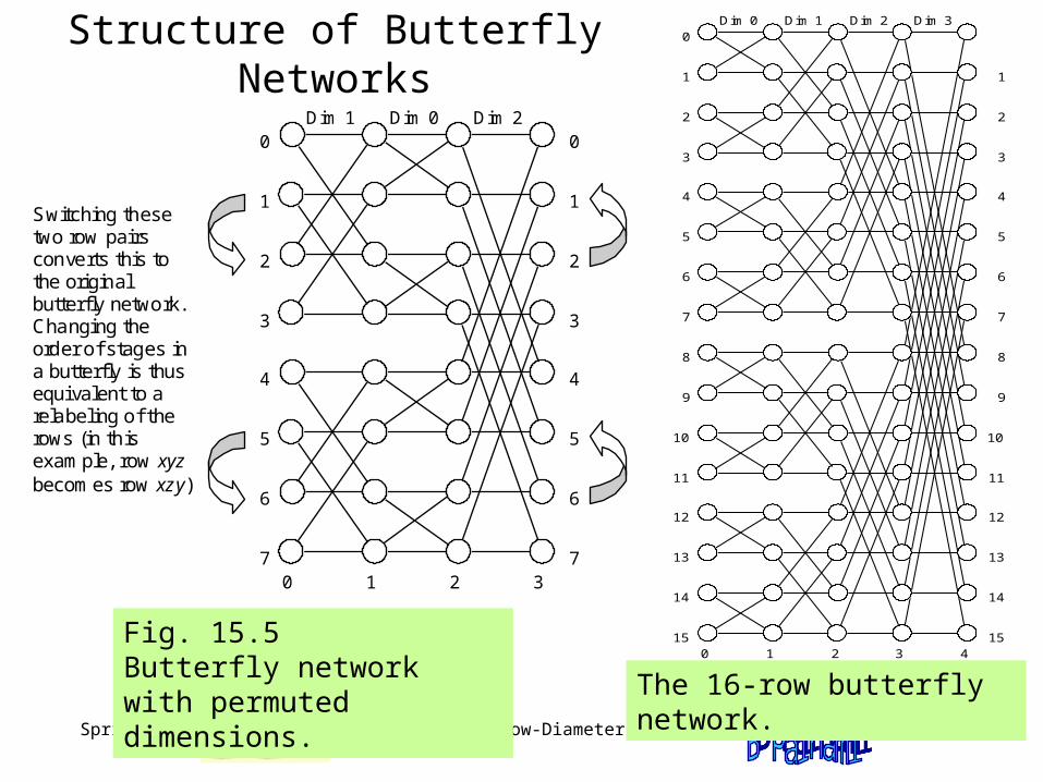
The 16-row butterfly network.

Fig. 15.5 Butterfly network with permuted dimensions.

0

1

2

3

4

5

6

7

0

1

2

3

4

5

6

7

Dim 1 Dim 0 Dim 2

0 1 2 3

Switching these two row pairs converts this to the original butterfly network. Changing the order of stages in a butterfly is thus equi valent to a relabeling of the rows (in this example, row xyz becomes row xzy)


Fat Trees

Fig. 15.6 Two representations of a fat tree.

P1

P0

P3

P4

P2P5

P7 P8

P6

Skinny tree?

0 1 2 3 4 5 6 7

0 2 4 6

0 4

0

Front view: Binary tree

Side view: Inverted binary tree

1 3 5 7

1 2 35 6 7

1 23 4 5 6 7

Fig. 15.7 Butterfly network redrawn as a fat tree.


Butterfly as Multistage Interconnection Network

Fig. 6.9 Example of a multistage memory access network

Generalization of the butterfly network High-radix or m-ary butterfly, built of m m switches Has mq rows and q + 1 columns (q if wrapped)

0 1 2 3log p Columns of 2-by-2 Switchesp Processors p Memory Banks

0000 0001 0010 0011 0100 0101 0110 0111 1000 1001 1010 1011 1100 1101 1110 1111

0 1 2 3 4 5 6 7 8 9 10 11 12 13 14 15

0000 0001 0010 0011 0100 0101 0110 0111 1000 1001 1010 1011 1100 1101 1110 1111

0 1 2 3 4 5 6 7 8 9 10 11 12 13 14 15

2 0 1 2 3log p + 1 Columns of 2-by-2 Switches

000 001 010 011 100 101 110 111 000 001 010 011 100 101 110 111

0 1 2 3 4 5 6 7 0 1 2 3 4 5 6 7

2

Fig. 15.8 Butterfly network used to connect modules that are on the same side


Beneš Network

Fig. 15.9 Beneš network formed from two back-to-back butterflies.

A 2q-row Beneš network: Can route any 2q 2q permutation It is “rearrangeable”

0 1 2 3 42 log p – 1 Columns of 2-by-2 Switches

000 001 010 011 100 101 110 111

0 1 2 3 4 5 6 7

Processors Memory Banks

000 001 010 011 100 101 110 111

0 1 2 3 4 5 6 7

2


Routing Paths in a Beneš Network

Fig. 15.10 Another example of a Beneš network.

0 1 2 3 4 5 6

2q + 1 Columns

0 1 2 3 4 5 6 7 8 9 10 11 12 13 14 15

2 Rows,q

0 1 2 3 4 5 6 7 8 9 10 11 12 13 14 15

2 Inputsq+1 2 Outputsq+1

To which memory modules can we connect proc 4 without rearranging the other paths?

What about proc 6?


15.3 Plus-or-Minus-2i Network

Fig. 15.11 Two representations of the eight-node PM2I network.

The hypercube is a subgraph of the PM2I network

±4

±10 1 2 3 4 5 6 7

±20

2

1

3

4

6

5

7


Unfolded PM2I Network

Fig. 15.12 Augmented data manipulator network.

Data manipulator network was used in Goodyear MPP, an early SIMD parallel machine.

“Augmented” means that switches in a column are independent, as opposed to all being set to same state (simplified control).

0 1 2 3

q + 1 Columns

0 1 2 3 4 5 6 7

0 1 2 3 4 5 6 7

2 Rowsq

a

b

a

b


15.4 The Cube-Connected Cycles Network

Fig. 15.13 A wrapped butterfly (left) converted into cube-connected cycles.

0

1

2

3

4

5

6

7

0

1

2

3

4

5

6

7

q columns/dimensions 0 1 2

0

1

2

3

4

5

6

7

Dim 1 Dim 2 Dim 0

0

1

2

3

4

5

6

7

q columns 1 2 3 = 0

2 rows q

The cube-connected cycles network (CCC) can be viewed as a simplified wrapped butterfly whose node degree is reduced from 4 to 3.


Another View of The CCC Network

Fig. 15.14 Alternate derivation of CCC from a hypercube.

0

2

1

3

4

6

5

7

0,00,1

0,2

1,0

4,2

2,1

Replacing each node of a high-dimensional q-cube by a cycle of length q is how CCC was originally proposed

Example of hierarchical substitution to derive a lower-cost network from a basis network


Emulation of Hypercube Algorithms by CCC

Node (x, j) is communicating along dimension j; after the next rotation, it will be linked to its dimension-(j + 1) neighbor.

Hypercube Dimension

q–1

3 2 1 0

Algorithm Steps0 1 2 3 . . .

.

.

.

Ascend

Descend

Normal

2 bitsm m bitsCycle ID = x Proc ID = y

N (x)

x, j–1

x, j

x, j+1

, j–1j–1

, j

, j+1

Dim j–1

Dim j

Dim j+1 , j–1

Cycle x

, j

N (x)

j+1

N (x)j+1

N (x)j

N (x)j

Fig. 15.15 CCC emulating a normal hypercube algorithm.

Ascend, descend, and normal algorithms.


15.5 Shuffle and Shuffle-Exchange Networks

Fig. 15.16 Shuffle, exchange, and shuffle–exchange connectivities.

0 1 2 3 4 5 6 7

0 1 2 3 4 5 6 7

0 1 2 3 4 5 6 7

000 001 010 011 100 101 110 111

0 1 2 3 4 5 6 7

0 1 2 3 4 5 6 7

0 1 2 3 4 5 6 7

Shuffle Exchange Shuffle-Exchange Alternate Structure

Unshuffle


Shuffle-Exchange Network

Fig. 15.17 Alternate views of an eight-node shuffle–exchange network.

0 1 2 3 4 5 6 7

0

1

2

3

4

5

6

7

SSE S

SE

S

SES

SE

SSE

S

SES

SE

S

SE


Routing in Shuffle-Exchange Networks

In the 2q-node shuffle network, node x = xq–1xq–2 . . . x2x1x0 is connected to xq–2 . . . x2x1x0xq–1 (cyclic left-shift of x)

In the 2q-node shuffle-exchange network, node x is additionally connected to xq–2 . . . x2x1x0x q–101011011 Source11010110 Destination^ ^^ ^ Positions that differ

01011011 Shuffle to 10110110 Exchange to 10110111 10110111 Shuffle to 01101111 01101111 Shuffle to 11011110 11011110 Shuffle to 1011110110111101 Shuffle to 01111011 Exchange to 01111010 01111010 Shuffle to 11110100 Exchange to 11110101 11110101 Shuffle to 1110101111101011 Shuffle to 11010111 Exchange to 11010110


Diameter of Shuffle-Exchange Networks

For 2q-node shuffle-exchange network: D = q = log2p, d = 4

With shuffle and exchange links provided separately, as in Fig. 15.18, the diameter increases to 2q – 1 and node degree reduces to 3

0 1 2 3 4 5 6 7

0

3

6

2

5

1

4

7

Exchange (dotted)

Shuffle (solid)

Fig. 15.18 Eight-node network with separate shuffle and exchange links.

ES

S

S

S

S

S S

S

E

E

E


Multistage Shuffle-

Exchange Network

Fig. 15.19 Multistage shuffle–exchange network (omega network) is the same as butterfly network.

0 1 2 3q + 1 Columns

0 1 2 3 4 5 6 7

0 1 2 3 4 5 6 7

0 1 2 3q + 1 Columns

0 1 2 3 4 5 6 7

0 1 2 3 4 5 6 7

0 1 2 3 4 5 6 7

0 1 2 3 4 5 6 7

0 1 2 3 4 5 6 7

0 1 2 3 4 5 6 7

q Columns q Columns0 1 2 0 1 2

A

A

A

A


15.6 That’s Not All, Folks!

D = log2 p + 1

d = (log2 p + 1)/2

B = p/4

When q is a power of 2, the 2qq-node cube-connected cycles network derived from the q-cube, by replacing each node with a q-node cycle, is a subgraph of the (q + log2q)-cube CCC is a pruned hypercube

Other pruning strategies are possible, leading to interesting tradeoffs

Fig. 15.20 Example of a pruned hypercube.

000

001

010

011

100

101

110

111

All dimension-0 links are kept

Even-dimension links are kept in the even subcube

Odd-dimension links are kept in the odd subcube


Möbius Cubes

Dimension-i neighbor of x = xq–1xq–2 ... xi+1xi ... x1x0 is:

xq–1xq–2 ... 0xi... x1x0 if xi+1 = 0 (xi complemented, as in q-cube)

xq–1xq–2 ... 1xi... x1x0 if xi+1 = 1 (xi and bits to its right complemented)

For dimension q – 1, since there is no xq, the neighbor can be defined in two possible ways, leading to 0- and 1-Mobius cubes

A Möbius cube has a diameter of about 1/2 and an average internode distance of about 2/3 of that of a hypercube

0

2

1

3

4

6

5

7

6

0-Mobius cube

0

2

1

3

7

4 5

1-Mobius cube

Fig. 15.21 Two 8-node Möbius cubes.


16 A Sampler of Other Networks

Complete the picture of the “sea of interconnection networks”:• Examples of composite, hybrid, and multilevel networks• Notions of network performance and cost-effectiveness


16.1 Performance Parameters for Networks

16.2 Star and Pancake Networks

16.3 Ring-Based Networks

16.4 Composite or Hybrid Networks

16.5 Hierarchical (Multilevel) Networks

16.6 Multistage Interconnection Networks


16.1 Performance Parameters for Networks

A wide variety of direct interconnection networks have been proposed for, or used in, parallel computers

They differ in topological, performance, robustness, and realizability attributes.

Fig. 4.8 (expanded)The sea of direct interconnection networks.


Diameter and Average DistanceDiameter D (indicator of worst-case message latency) Routing diameter D(R); based on routing algorithm R

Average internode distance (indicator of average-case latency) Routing average internode distance (R)

For the 3 3 mesh: = (4 18 + 4 15

+12)

/ (9 8) = 2 [or 144 / 81 = 16 / 9]

Finding the average internode distance of a 3 3 mesh.

P P P

P P P

P P P

0 1 2

3 4 5

6 7 8

Sum of distances from corner node: 2 1 + 3 2 + 2 3 + 1 4 = 18

Sum of distances from side node: 3 1 + 3 2 + 2 3 = 15

Sum of distances from center node: 4 1 + 4 2 = 12 Average distance:

(4 18 + 4 15 + 1 12) / (9 x 8) = 2

For the 3 3 torus: = (4 1 + 4 2) / 8 = 1.5 [or 12 / 9 = 4 / 3]


Bisection Width31

30

29

0 1 2

3

4

5

6

7

8

9

20

21

22

23

24

25

26

27

28

10

11

12

13

14 15 16 17

18

19

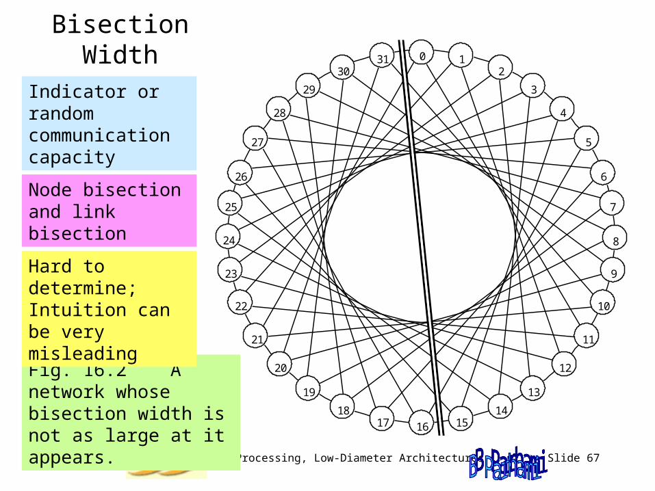
Fig. 16.2 A network whose bisection width is not as large at it appears.

Node bisection and link bisection

Indicator or random communication capacity

Hard to determine; Intuition can be very misleading


Determining the Bisection Width

Establish upper bound by taking a number of trial cuts.Then, try to match the upper bound by a lower bound.

Establishing a lower bound on B:

Embed Kp into p-node network

Let c be the maximum congestion

B p2/4/c

P 0 P 1 P 2

P 3 P 4 P 5

P 6 P 7 P 8

0 1 2

3 4 5

6 7 8

7

7

An embedding of K into 3 3 mesh 9

P 0

P 1

P 2

P 3

P 4 P 5

P 6

P 7

P 8

Bisection width = 4 5 = 20

K 9


Degree-Diameter Relationship

Age-old question: What is the best way to interconnect p nodes of degree d to minimize the diameter D of the resulting network?

Alternatively: Given a desired diameter D and nodes of degree d, what is the max number of nodes p that can be accommodated?

Moore bounds (digraphs)

p 1 + d + d2 + . . . + dD = (dD+1 – 1)/(d – 1)

D logd [p(d – 1) + 1] – 1

Only ring and Kp match these bounds x

d nodesd

2 nodes

Moore bounds (undirected graphs)

p 1 + d + d(d – 1) + . . . + d(d – 1)D–1 = 1 + d [(d – 1)D – 1]/(d – 2)D logd–1[(p – 1)(d – 2)/d + 1]

Only ring with odd size p and a few other networks match these bounds

x

d nodesd (d – 1) nodes


Moore Graphs

A Moore graph matches the bounds on diameter and number of nodes.

For d = 2, we have p 2D + 1Odd-sized ring satisfies this bound

11010

01101

1001111100

00111

11001

10101

10110

0111001011

Fig. 16.1 The 10-node Petersen graph.

For d = 3, we have p 3 2D – 2 D = 1 leads to p 4 (K4 satisfies the bound)D = 2 leads to p 10 and the first nontrivial example (Petersen graph)


How Good Are Meshes and Hypercubes?

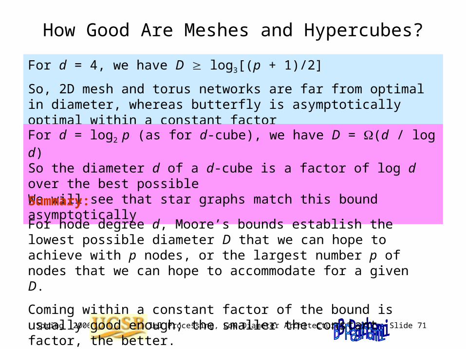
For d = 4, we have D log3[(p + 1)/2]

So, 2D mesh and torus networks are far from optimal in diameter, whereas butterfly is asymptotically optimal within a constant factor

For d = log2 p (as for d-cube), we have D = (d / log d) So the diameter d of a d-cube is a factor of log d over the best possibleWe will see that star graphs match this bound asymptotically

Summary:

For node degree d, Moore’s bounds establish the lowest possible diameter D that we can hope to achieve with p nodes, or the largest number p of nodes that we can hope to accommodate for a given D.

Coming within a constant factor of the bound is usually good enough; the smaller the constant factor, the better.


Layout Area and Longest Wire

The VLSI layout area required by an interconnection network is intimately related to its bisection width B

The longest wire required in VLSI layout affects network performance

For example, any 2D layout of a p-node hypercube requires wires of length ((p / log p)1/2); wire length of a mesh does not grow with size

When wire length grows with size, the per-node performance is bound to degrade for larger systems, thus implying sublinear speedup

If B wires must cross the bisection in 2D layout of a network and wire separation is 1 unit, the smallest dimension of the VLSI chip will be B

The chip area will thus be (B2) units p-node 2D mesh needs O(p) area p-node hypercube needs at least (p2) area

B wires crossing a bisection


Measures of Network Cost-Effectiveness

Composite measures, that take both the network performance and its implementation cost into account, are useful in comparisons

Robustness must be taken into account in any practical comparison of interconnection networks (e.g., tree is not as attractive in this regard)

One such measure is the degree-diameter product, dD

Mesh / torus: (p1/2)Binary tree: (log p)Pyramid: (log p)Hypercube: (log2 p)

However, this measure is somewhat misleading, as the node degree d is not an accurate measure of cost; e.g., VLSI layout area also depends on wire lengths and wiring pattern and bus based systems have low node degrees and diameters without necessarily being cost-effective

Not quite similar in cost-performance


16.2 Star and Pancake Networks

Fig. 16.3 The four-dimensional star graph.

Has p = q ! nodes

Each node labeled with a string x1x2 ... xq which is a permutation of {1, 2, ... , q}

Node x1x2 ... xi ... xq is connected to xi x2 ... x1 ... xq for each i (note that x1 and xi are interchanged)

When the i th symbol is switched with x1 , the corresponding link is called a dimension-i link

d = q – 1; D = 3(q – 1)/2

D, d = O(log p / log log p)

1234 4231

2134 3241 2431

3421

4321

2413

234131241324

2314

3214

1423

4123

2143

1243

4213

3142

1342

4312

1432

4132

3412

3

2

3 2

3

2

4


Routing in the Star Graph

Source node 1 5 4 3 6 2 Dimension-2 link to 5 1 4 3 6 2 Dimension-6 link to 2 1 4 3 6 5 Last symbol now adjusted Dimension-2 link to 1 2 4 3 6 5 Dimension-5 link to 6 2 4 3 1 5 Last 2 symbols now adjusted Dimension-2 link to 2 6 4 3 1 5 Dimension-4 link to 3 6 4 2 1 5 Last 3 symbols now adjusted Dimension-2 link to 6 3 4 2 1 5 Dimension-3 link to 4 3 6 2 1 5 Last 4 symbols now adjusted Dimension-2 link (Dest’n) 3 4 6 2 1 5

We need a maximum of two routing steps per symbol, except that last two symbols need at most 1 step for adjustment D 2q – 3

The diameter of star is in fact somewhat less D = 3(q – 1)/2

Clearly, this is not a shortest-path routing algorithm.

Correction to text, p. 328: diameter is not 2q – 3


Star’s Sublogarithmic Degree and Diameter

d = (q) and D = (q); but how is q related to the number p of nodes?

p = q ! e–qqq (2q)1/2 [ using Striling’s approximation to q ! ]

ln p –q + (q + 1/2) ln q + ln(2)/2 = (q log q) or q = (log p / log log

p)Hence, node degree and diameter are sublogarithmic

Star graph is asymptotically optimal to within a constant factor with regard to Moore’s diameter lower bound

Routing on star graphs is simple and reasonably efficient; however, virtually all other algorithms are more complex than the corresponding algorithms on hypercubes

Network diameter 4 5 6 7 8 9Star nodes 24 -- 120 720 -- 5040Hypercube nodes 16 32 64 128 256 512


The Star-Connected Cycles Network

Fig. 16.4 The four-dimensional star-connected cycles network.

Replace degree-(q – 1) nodes with (q – 1)-cycles

This leads to a scalable version of the star graph whose node degree of 3 does not grow with size

The diameter of SCC is about the same as that of a comparably sized CCC network

However, routing and other algorithms for SCC are more complex

1234,4

3

2

3 2

3

21234,3

41234,2


Pancake Networks

Similar to star networks in terms of node degree and diameter

Dimension-i neighbor obtained by “flipping” the first i symbols; hence, the name “pancake”

1234

21343214

4321Dim 2

Dim 3

Dim 4

Source node 1 5 4 3 6 2 Dimension-2 link to 5 1 4 3 6 2 Dimension-6 link to 2 6 3 4 1 5Last 2 symbols now adjusted Dimension-4 link to 4 3 6 2 1 5Last 4 symbols now adjusted Dimension-2 link (Dest’n) 3 4 6 2 1 5

We need two flips per symbol in the worst case; D 2q – 3


Cayley Networks

Group:

A semigroup with an identity element and inverses for all elements.

Example 1: Integers with addition or multiplication operator form a group.

Example 2: Permutations, with the composition operator, form a group.

Node x

x 1

x 2

x 3Gen 1

Gen 2

Gen 3

Star and pancake networks are instances of Cayley graphs

Cayley graph:

Node labels are from a group G, and a subset S of G defines the connectivity via the group operator

Node x is connected to node y iff x = y for some S

Elements of S are “generators” of G if every element of G can be expressed as a finite product of their powers


Star as a Cayley Network

Fig. 16.3 The four-dimensional star graph.

Four-dimensional star:

Group G of the permutations of {1, 2, 3, 4}

The generators are the following permutations:(1 2) (3) (4)(1 3) (2) (4)(1 4) (2) (3)

The identity element is:(1) (2) (3) (4)

1234 4231

2134 3241 2431

3421

4321

2413

234131241324

2314

3214

1423

4123

2143

1243

4213

3142

1342

4312

1432

4132

3412

3

2

3 2

3

2

4(1 4) (2) (3)

(1 3) (2) (4)


16.3 Ring-Based Networks

Fig. 16.5 A 64-node ring-of-rings architecture composed of eight 8-node local rings and one second-level ring.

Rings are simple, but have low performance and lack robustness

Message source

Local RingRemote Ring

S

D

Message destination

Hence, a variety of multilevel and augmented ring networks have been proposed


Chordal Ring Networks

Fig. 16.6 Unidirectional ring, two chordal rings, and node connectivity in general.

Given one chord type s, the optimal length for s is approximately p1/2

0

4

26

7

3

1

5

0

4

26

7

3

1

5

(a) (b)

v 0

4

26

7

3

1

5

(b)(a)

v+1v–1

v+s

v+sv–s

v–s 1

k–1k–1

1

s k–1

s 1.

. ..

..

s =10v 0

4

26

7

3

1

5

(b)(a)

v+1v–1

v+s

v+sv–s

v–s 1

k–1k–1

1

s k–1

s 1.

. ..

..

s =10

( a )

( d ) ( c )

( b )

Routing algorithm: Greedy routing


Chordal Rings Compared to Torus Networks

Fig. 16.7 Chordal rings redrawn to show their similarity to torus networks.

The ILLIAC IV interconnection scheme, often described as 8 8 mesh or torus, was really a 64-node chordal ring with skip distance 8.

0 1 2

3

6 7

4 5

0 1 2

3

6 7

4

8

5

A class of chordal rings, recently studied at UCSB (two-part paper in IEEE TPDS, August 2005) have a diameter of D = 2

Perfect difference {0, 1, 3}: All numbers in the range 1-6 mod 7 can be formed as the difference of two numbers in the set.

Perfect Difference Networks


Periodically Regular Chordal Rings

Fig. 16.8 Periodically regular chordal ring.

Modified greedy routing: first route to the head of a group; then use pure greedy routing

0

4

26

7

3

1

5

Group 0

s1s0

s0

s2

Group 0

Group 1

Group 2

Group p/g – 1

Group i

Nodes 0 to g – 1

Nodes g to 2g – 1

Nodes 2g to 3g – 1

Nodes ig to (i+1)g – 1

Nodes p – g to p – 1

A skip link leads to the same relative position in the destination group


Some Properties of PRC Rings

Fig. 16.9 VLSI layout for a 64-node periodically regular chordal ring.

0

1

2

3

4

5

63

6

7To 3To 6

Remove some skip links for cost-performance tradeoff; similar in nature to CCC network with longer cycles

Fig. 16.10 A PRC ring redrawn as a butterfly- or ADM-like network.

31 30 29

0 1 2 3

4 5 6 7

8 9

20 21 22 23

24 25 26 27

28

10 11

12 13 14 15

16 17 18 19

Dimension 1 s = nil

Dimension 2 s = 4

Dimension 1 s = 8

Dimension 1 s = 16

No skip in this dimension

1

2

3

4

b

a

d

c

f

e g

b

a

d

c

f

e

g


16.4 Composite or Hybrid Networks

Motivation: Combine the connectivity schemes from two (or more) “pure” networks in order to:

Achieve some advantages from each structure

Derive network sizes that are otherwise unavailable

Realize any number of performance / cost benefits

A very large set of combinations have been tried

New combinations are still being discovered


Composition by Cartesian Product Operation

Fig. 13.4 Examples of product graphs.

Properties of product graph G = G G:

Nodes labeled (x , x ), x V , x V

p = pp d = d + d D = D + D = +

Routing: G -first (x , x ) (y , x ) (y , y )

Broadcasting

Semigroup & parallel prefix computations

=3-by-2 torus

=

=

0

1

2

a

b

0a

1a

2a0b

1b

2b


Other Properties and Examples of Product Graphs

Fig. 16.11 Mesh of trees compared with mesh-connected trees.

If G and G are Hamiltonian, then the p p torus is a subgraph of G For results on connectivity and fault diameter, see [Day00], [AlAy02]

Mesh of trees (Section 12.6) Product of two trees


16.5 Hierarchical (Multilevel) Networks

Can be defined from the bottom up or from the top down

We have already seen several examples of hierarchical networks: multilevel buses (Fig. 4.9); CCC; PRC rings

Fig. 16.13 Hierarchical or multilevel bus network.

Take first-level ring networks and interconnect them as a hypercube

Take a top-level hypercube and replace its nodes with given networks


Example: Mesh of Meshes Networks

EW

N

S

Fig. 16.12 The mesh of meshes network exhibits greater modularity than a mesh.

The same idea can be used to form ring of rings, hypercube of hypercubes, complete graph of complete graphs, and more generally, X of Xs networks

When network topologies at the two levels are different, we have X of Ys networks

Generalizable to three levels (X of Ys of Zs networks), four levels, or more


Example: Swapped Networks

Two-level swapped network with 2 2 mesh as its nucleus.

0 1

2 3

Level-1 link

00 10

20 30

01 11

21 31

02 12

22 32

03 13

23 33

Level-2 link

Build a p2-node network using p-node building blocks (nuclei or clusters) by connecting node i in cluster j to node j in cluster i

Cluster # Node #

Cluster # Node #

We can square the network size by adding one link per node

Also known in the literature as OTIS (optical transpose interconnect system) network


16.6 Multistage Interconnection Networks

Numerous indirect or multistage interconnection networks (MINs) have been proposed for, or used in, parallel computers

They differ in topological, performance, robustness, and realizability attributes

We have already seen the butterfly, hierarchical bus, beneš, and ADM networks

Fig. 4.8 (modified)The sea of indirect interconnection networks.


Self-Routing Permutation Networks

Do there exist self-routing permutation networks? (The butterfly network is self-routing, but it is not a permutation network)

Permutation routing through a MIN is the same problem as sorting

Fig. 16.14 Example of sorting on a binary radix sort network.

7 (111) 0 (000) 4 (100) 6 (110) 1 (001) 5 (101) 3 (011) 2 (010)

7 (111)

0 (000)

4 (100)

6 (110)

1 (001)

5 (101)

3 (011)

2 (010)

0 1 3 2

5

7 4 6

0 1 3 2

6

4 5 7

Sort by MSB

Sort by LSB

Sort by the middle bit


Partial List of Important MINs

Augmented data manipulator (ADM): aka unfolded PM2I (Fig. 15.12)

Banyan: Any MIN with a unique path between any input and any output (e.g. butterfly)

Baseline: Butterfly network with nodes labeled differently

Beneš: Back-to-back butterfly networks, sharing one column (Figs. 15.9-10)

Bidelta: A MIN that is a delta network in either direction

Butterfly: aka unfolded hypercube (Figs. 6.9, 15.4-5)

Data manipulator: Same as ADM, but with switches in a column restricted to same state

Delta: Any MIN for which the outputs of each switch have distinct labels (say 0 and 1

for 2 2 switches) and path label, composed of concatenating switch output labels

leading from an input to an output depends only on the output

Flip: Reverse of the omega network (inputs outputs)

Indirect cube: Same as butterfly or omega

Omega: Multi-stage shuffle-exchange network; isomorphic to butterfly (Fig. 15.19)

Permutation: Any MIN that can realize all permutations

Rearrangeable: Same as permutation network

Reverse baseline: Baseline network, with the roles of inputs and outputs interchanged

spring 2006parallel processing, low-diameter architecturesslide 1 part iv low-diameter architectures

Documents