Featuring:• Analyzing Mixers Using Intermodulation Distortion Analysis• The FFT Window• Monte Carlo Tolerances and Distributions

Applications for Micro-Cap™ Users

Spring 2012News

Intermodulation Distortion Analysis

�

News In Preview

This newsletter's Q and A section describes how to get MC8 running on Windows 7.

This newsletter's Easily Overlooked section describes how to use the Change Attributes command to quickly alter attributes for a part or all of an entire circuit.

The first article describes how to analyze mixers using Intermodulation Distortion analysis. It includes an example of a singly-balanced diode mixer. The second article describes the use of the FFT Window for plotting frequency spectra using the Ua709 schematic as an example.

The third article describes the meaning of LOT and DEV and how these tolerances are computed in Monte Carlo simulations.

Contents

News In Preview .................................................................................................................................................2Book Recommendations ....................................................................................................................................3Micro-Cap Questions and Answers .................................................................................................................4Easily Overlooked Features ...............................................................................................................................5Analyzing Mixers Using Intermodulation Distortion Analysis....................................................................6The FFT Window ...............................................................................................................................................9Monte Carlo Tolerances and Distributions ...................................................................................................13Product Sheet .....................................................................................................................................................16

�

Book Recommendations

General SPICE• Computer-Aided Circuit Analysis Using SPICE, Walter Banzhaf, Prentice Hall 1989. ISBN# 0-13-162579-9

• Macromodeling with SPICE, Connelly and Choi, Prentice Hall 1992. ISBN# 0-13-544941-3

• Inside SPICE-Overcoming the Obstacles of Circuit Simulation, Ron Kielkowski, McGraw-Hill, 1993. ISBN# 0-07-911525-X

• The SPICE Book, Andrei Vladimirescu, John Wiley & Sons, Inc., 1994. ISBN# 0-471-60926-9

MOSFET Modeling• MOSFET Models for SPICE Simulation, William Liu, Including BSIM3v3 and BSIM4, Wiley-Interscience, ISBN# 0-471-39697-4

Signal Integrity• Signal Integrity and Radiated Emission of High-Speed Digital Signals, Spartaco Caniggia, Francescaromana Maradei, A John Wiley and Sons, Ltd, First Edition, 2008 ISBN# 978-0-470-51166-4

Micro-Cap - Czech• Resime Elektronicke Obvody, Dalibor Biolek, BEN, First Edition, 2004. ISBN# 80-7300-125-X

Micro-Cap - German• Simulation elektronischer Schaltungen mit MICRO-CAP, Joachim Vester, Verlag Vieweg+Teubner, First Edition, 2010. ISBN# 978-3-8348-0402-0

Micro-Cap - Finnish• Elektroniikkasimulaattori, Timo Haiko, Werner Soderstrom Osakeyhtio, 2002. ISBN# 951-0-25672-2

Design• High Performance Audio Power Amplifiers, Ben Duncan, Newnes, 1996. ISBN# 0-7506-2629-1

• Microelectronic Circuits, Adel Sedra, Kenneth Smith, Fourth Edition, Oxford, 1998

High Power Electronics• Power Electronics, Mohan, Undeland, Robbins, Second Edition, 1995. ISBN# 0-471-58408-8

• Modern Power Electronics, Trzynadlowski, 1998. ISBN# 0-471-15303-6 Switched-Mode Power Supply Simulation • SMPS Simulation with SPICE 3, Steven M. Sandler, McGraw Hill, 1997. ISBN# 0-07-913227-8

• Switch-Mode Power Supplies Spice Simulations and Practical Designs, Christophe Basso, McGraw-Hill 2008. This book describes many of the SMPS models supplied with Micro-Cap.

�

Micro-Cap Questions and Answers

Question: I am trying to reinstall Micro-Cap 8 on a system that has Windows 7. Will it work? I haven't had much luck so far getting it installed.

Answer: Yes, Micro-Cap 8 will run on Windows 7 but you must so several things first.

1) Install MC8 from your original CD.

You only need to do this if the system is new and does not already have an MC8 installed.

We strongly recommend that you install MC8 in a non-write-protected directory like C:\MC8. Do not Install it in the Program Files folder because many Windows 7 installations write-protect the Program Files folder and MC8 must write to data files in the installation folder.

2) Download and install the newest Hasp driver (Haspdinst.exe.).

You can do that here:

http://www.spectrum-soft.com/download.shtm

Follow the instructions on the web page for installing Haspdinst.exe.

3) Try running MC8. If it runs you are finished. Otherwise you need to download the latest MC8 zip file.

To access the file you will need a user name and password which Spectrum Software will email to you when we receive an email request for the user name and password. Be sure to include your name and key ID number. Send email requests to:

support@spectrum-soft.com

Uncompress the downloaded MC8.EXE to the MC8 folder overwriting the MC8.EXE file there.

�

Easily Overlooked Features

This section is designed to highlight one or two features per issue that may be overlooked among all the capabilities of Micro-Cap.

Change CommandThe Change command, which is available under the Edit menu, provides an easy means of changing a variety of items. Here we'll concentrate on just one of the Change commands, Change Attributes. The dialog box shown below lets you delete, change, show, or hide any component attribute.

For example, suppose you wanted to change the color of the R1 and R2 RESISTANCE attribute text to red. The settings below show how this would be done.

You can use the Change Value option to change the value of any attribute like the MODEL attribute of some or all of the NPN devices in the circuit.

You can use the Hide and Show options to hide or show either the attribute's NAME or VALUE. This is often useful if you wish to hide part names to simplify the schematic for some purpose other than simulation.

The Change command is very useful for changing the attribute font, say for example, if you prefer Verdana to Arial for value attributes.

Fig. 1 - Change dialog box

You can also add or delete any optional attributes such as COST, POWER, SHAPEGROUP or any user-added attribute. Try experimenting with the Change command. You'll find it a powerful and flexible tool.

�

Analyzing Mixers Using Intermodulation Distortion Analysis

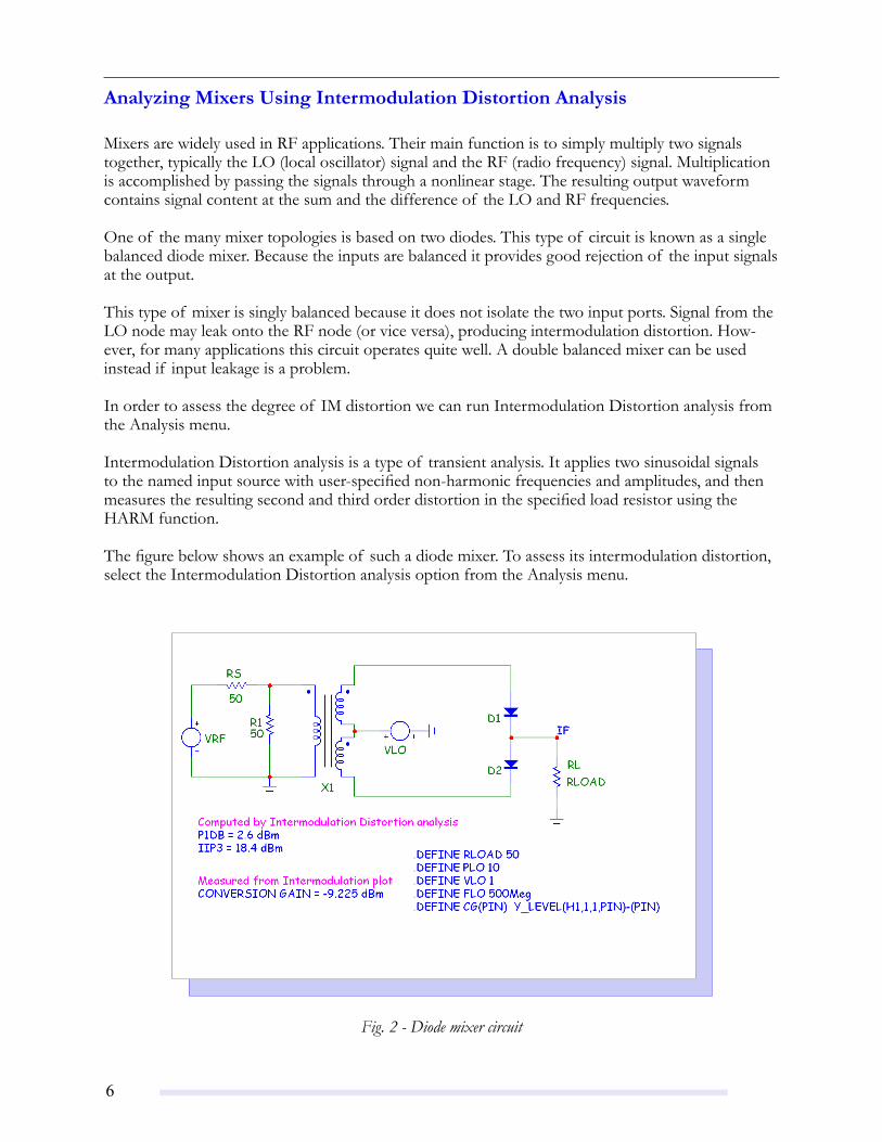
Mixers are widely used in RF applications. Their main function is to simply multiply two signals together, typically the LO (local oscillator) signal and the RF (radio frequency) signal. Multiplication is accomplished by passing the signals through a nonlinear stage. The resulting output waveform contains signal content at the sum and the difference of the LO and RF frequencies.

One of the many mixer topologies is based on two diodes. This type of circuit is known as a single balanced diode mixer. Because the inputs are balanced it provides good rejection of the input signals at the output.

This type of mixer is singly balanced because it does not isolate the two input ports. Signal from the LO node may leak onto the RF node (or vice versa), producing intermodulation distortion. How-ever, for many applications this circuit operates quite well. A double balanced mixer can be used instead if input leakage is a problem.

In order to assess the degree of IM distortion we can run Intermodulation Distortion analysis from the Analysis menu.

Intermodulation Distortion analysis is a type of transient analysis. It applies two sinusoidal signals to the named input source with user-specified non-harmonic frequencies and amplitudes, and then measures the resulting second and third order distortion in the specified load resistor using the HARM function.

The figure below shows an example of such a diode mixer. To assess its intermodulation distortion, select the Intermodulation Distortion analysis option from the Analysis menu.

Fig. 2 - Diode mixer circuit

�

Its analysis limits menu looks like this:

Fig. 3 - Analysis Limits dialog for Distortion Analysis

The system will apply the specified two frequencies, 400MHz and 450MHz, to the source named VRF. Its voltage will be log stepped from 50mV to 1.0V. The VLO source will use the frequency and voltage level specified in the schematic (1 Volt and 500MHz)

Press F2 to start the run and in a few seconds the following plot will appear.

Fig. 4 - Distortion plot

�

Fig. 5 - Working plot window

This shows a plot of the H1 harmonic in blue and IM3 (3’rd order intermodulation) in green. The program will find the region on the H1 plot where the slope is closest to 1.0 and also on the IM3 plot where the slope is closest to 3.0. It will then draw lines of slope 1.0 and 3.0 respectively, and compute where they intersect. That point of intersection is the IP3 point. It also computes and marks the point where the H1 curve drops by 1dB from the ideal slope=1 line. Both of these are important figures of merit for a mixer.

In this case the values are P1dBm=2.6 and IP3=18.4.

The second plot window holds plots of the waveforms which are used to compute the distortion and harmonic variables. The program applies the FFT to these basic waveforms and computes the necessary distortion plot values. This "working plot window" looks like this.

Here we've plotted the following waveforms.

HARM(V(RL)) The frequency spectrum of the output voltage waveform V(RL)V(RL) The output waveformHARM(I(VRF)) The frequency spectrum of the input current waveform V(RL)HARM(V(VRF)) The frequency spectrum of the RF input voltage waveformHARM(V(VLO)) The frequency spectrum of the LO voltage waveform

Not all of these are necessary. The later two are for information only to show what spectra are actu-ally applied during the run.

�

The FFT Window

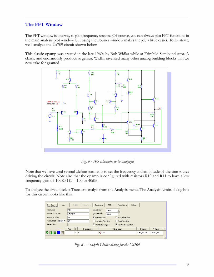
The FFT window is one way to plot frequency spectra. Of course, you can always plot FFT functions in the main analysis plot window, but using the Fourier window makes the job a little easier. To illustrate, we'll analyze the Ua709 circuit shown below.

This classic opamp was created in the late 1960s by Bob Widlar while at Fairchild Semiconductor. A classic and enormously productive genius, Widlar invented many other analog building blocks that we now take for granted.

Fig. 6 - 709 schematic to be analyzed

Note that we have used several .define statments to set the frequency and amplitude of the sine source driving the circuit. Note also that the opamp is configured with resistors R10 and R11 to have a low frequency gain of 100K/1K = 100 or 40dB.

To analyze the circuit, select Transient analyis from the Analysis menu. The Analysis Limits dialog box for this circuit looks like this.

Fig. 6 - Analysis Limits dialog for the Ua709

10

Fig. 7 - FFT window for the 709 circuit

Note that we have specified a Time Range of 5/F0 = 5/1K = 5ms. Since F0 is the frequency of the driving source the run will be for 5mS and the Fourier frequency resolution will be 1/5mS or 200 Hz. Note also that we have specified the Maximum Time Step as .001*1/F0, which insures sufficient ac-curacy. The use of .define statements like this lets you easily change the input frequency setings and have the simulation run adjust accordingly. Press F2 and when the run is finished, select Transient menu / FFT Windows / Add FFT Window. The display will show the FFT Properties dialog. Click on the FFT tab and type 50 into the Autoscale First ____ Harmonics field. The display should now look like this.

The window displays a plot of the dB value of the first 50 frequency values (50*200Hz=10KHz). Of these, only multiples of F0 = 1KHz are significantly different from zero. Their values are as follows.

1KHz -0.111dB2KHz -84.509dB3KHz -104.665dB4KHz -143.815dB5KHz -173.725dB

There is no measurable value for higher harmonics. Is that all there is? Can no more information be squeezed from the run? As it is no more can be gained. To see the spectra with greater accuracy we can do another run using a smaller time step. To illustrate the effect, set the Maximum Time Step to .0001*1/F0 or 10 times smaller than the last run. Now the plot looks like Figure 8.

11

Fig. 8 - FFT window for the circuit run with a smaller time step

The values of the 6'th and 7'th harmonics are now visible.

1KHz -0.111dB2KHz -84.509dB3KHz -104.662dB4KHz -149.932dB5KHz -171.883dB6KHz -204.570dB7KHz -230.253dB

The FFT routines are resolving a signal difference of about 230 dB, or a little better than 11 decimal places. In particular the FFT is picking out a 1E-11 volt 7KHz signal out of a signal that contains a 1.0 volt 1KHz signal.

Note that the smaller timestep slightly changes the values of harmonics 3, 4, and 5. Usually this high a degree of accuracy is not required and a maximum time step of .001*F0 is more than adequate. In many cases, even .01*F0 is adequate for a rough estimate.

One thing to remember is that to reach the FFT Properties dialog you must first select the FFT window by clicking on it. Normally after every run, the analysis plot is set to be the selected window. So if you merely press F10 you'll get the Properties dialog box for the analysis plot, not the FFT window plot.

We've used the default FFT window settings except for the number of harmonics to be plotted, where we asked for 50 instead of the default value of 10. What other changes could we have made? To see, click on the FFT window, then press F10 to invoke the Properties dialog box. Click on the Plot tab and select Harm under the What To Plot panel. This produces a plot that is similar to the one above except that we're plotting the actual value of the spectra, not the dB representation. The vertical scale has been changed from linear to log so the shape of the plot is very similar to the last one. The vertical scale is annotated in powers of ten not in dB units.

1�

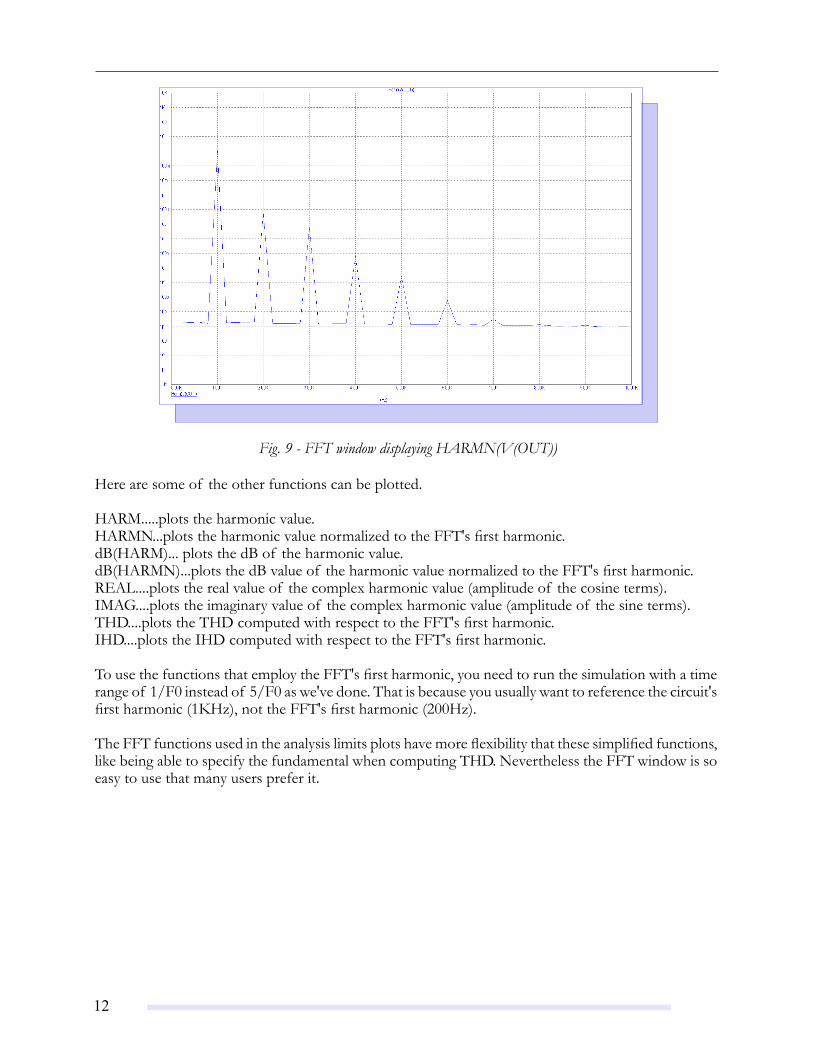
Here are some of the other functions can be plotted.

HARM.....plots the harmonic value.HARMN...plots the harmonic value normalized to the FFT's first harmonic.dB(HARM)... plots the dB of the harmonic value.dB(HARMN)...plots the dB value of the harmonic value normalized to the FFT's first harmonic.REAL....plots the real value of the complex harmonic value (amplitude of the cosine terms).IMAG....plots the imaginary value of the complex harmonic value (amplitude of the sine terms).THD....plots the THD computed with respect to the FFT's first harmonic.IHD....plots the IHD computed with respect to the FFT's first harmonic.

To use the functions that employ the FFT's first harmonic, you need to run the simulation with a time range of 1/F0 instead of 5/F0 as we've done. That is because you usually want to reference the circuit's first harmonic (1KHz), not the FFT's first harmonic (200Hz).

The FFT functions used in the analysis limits plots have more flexibility that these simplified functions, like being able to specify the fundamental when computing THD. Nevertheless the FFT window is so easy to use that many users prefer it.

Fig. 9 - FFT window displaying HARMN(V(OUT))

1�

Monte Carlo Tolerances and Distributions

Several recent requests about the nature of the Monte Carlo LOT and DEV tolerances have prompted us to include an article on the subject.

In Micro-Cap both absolute (LOT) and relative (DEV) tolerances can be applied. A LOT tolerance is first applied to each device which uses the same model statement. A DEV tolerance is then added to the first through last device relative to the LOT toleranced value originally chosen for the first device. In other words, the first device in the list receives a LOT tolerance, if one was specified. All devices, including the first, then receive the first device's value plus or minus the DEV tolerance. DEV toler-ances provide a means for having some devices track in their critical parameter values.

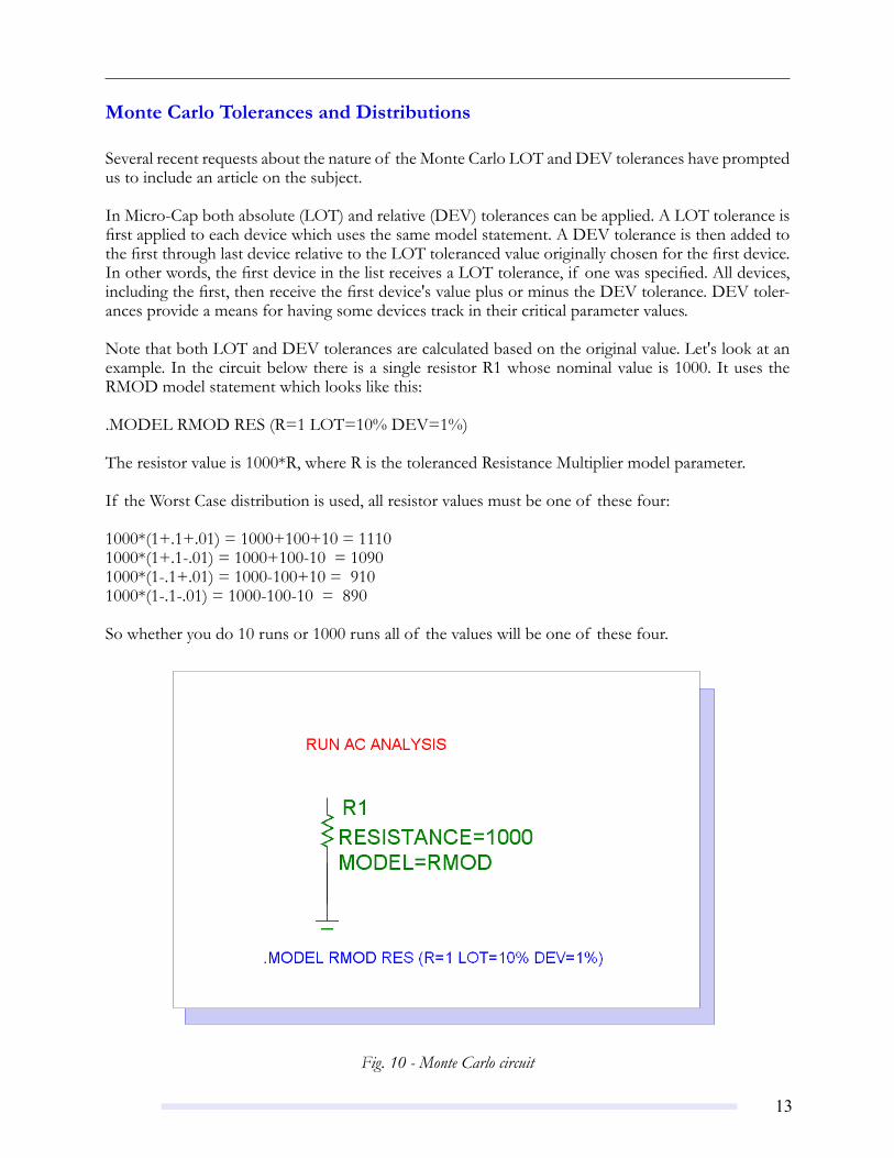
Note that both LOT and DEV tolerances are calculated based on the original value. Let's look at an example. In the circuit below there is a single resistor R1 whose nominal value is 1000. It uses the RMOD model statement which looks like this:

.MODEL RMOD RES (R=1 LOT=10% DEV=1%)

The resistor value is 1000*R, where R is the toleranced Resistance Multiplier model parameter.

If the Worst Case distribution is used, all resistor values must be one of these four:

1000*(1+.1+.01) = 1000+100+10 = 11101000*(1+.1-.01) = 1000+100-10 = 10901000*(1-.1+.01) = 1000-100+10 = 9101000*(1-.1-.01) = 1000-100-10 = 890

So whether you do 10 runs or 1000 runs all of the values will be one of these four.

Fig. 10 - Monte Carlo circuit

1�

To illustrate how this works, run AC analysis. Its Analysis Limits dialog box looks like this.

Here we are plotting just the resistance of R1. We are using just two data points per run to speed things up. As the resistance doesn't vary with frequency, what we'll see is a set of horizontal lines whose Y value equals the resistance computed for that run. Here is what the 40 runs look like.

Fig. 11 - AC Analysis Limits dialog for circuit

Fig. 12 - The analysis run

As expected, we see four horizontal lines representing the resistance values of the 40 runs. The reason there are only four is that using a Worst Case distribution with a LOT and DEV tolerance only four values are possible. To see this in a Monte Carlo sense, look at Figure 13, which shows the histogram and a list of the resistance values.

1�

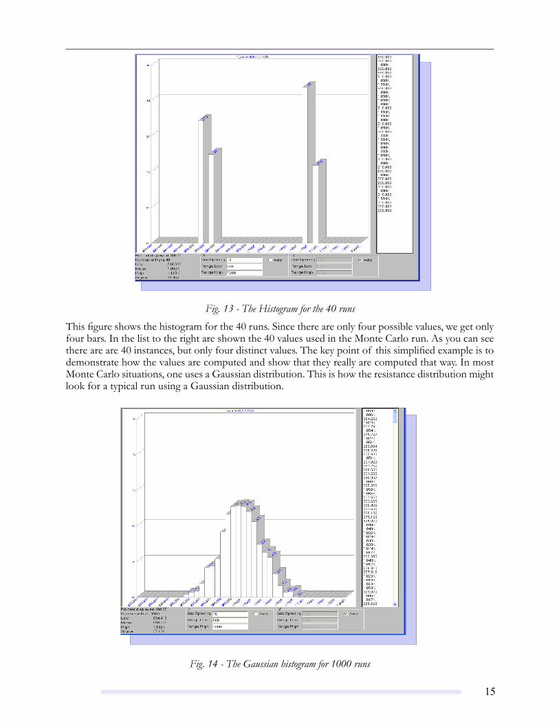
Fig. 13 - The Histogram for the 40 runs

This figure shows the histogram for the 40 runs. Since there are only four possible values, we get only four bars. In the list to the right are shown the 40 values used in the Monte Carlo run. As you can see there are are 40 instances, but only four distinct values. The key point of this simplified example is to demonstrate how the values are computed and show that they really are computed that way. In most Monte Carlo situations, one uses a Gaussian distribution. This is how the resistance distribution might look for a typical run using a Gaussian distribution.

Fig. 14 - The Gaussian histogram for 1000 runs

1�

Product Sheet

Latest Version numbersMicro-Cap 10 .......................................................................Version 10.0.8.0Micro-Cap 9 .........................................................................Version 9.0.8Micro-Cap 8 .........................................................................Version 8.1.3Micro-Cap 7 .........................................................................Version 7.2.4

Spectrum’s numbersSales .......................................................................................(408) 738-4387Technical Support ...............................................................(408) 738-4389FAX ......................................................................................(408) 738-4702Email sales ............................................................................sales@spectrum-soft.comEmail support ......................................................................support@spectrum-soft.comWeb Site ................................................................................http://www.spectrum-soft.comUser Group ..........................................................................micro-cap-subscribe@yahoogroups.com