SRN Model for IEEE 802.11 DCF MAC Protocol in Multi-hop Ad Hoc Networks with Hidden Nodes

Osama Younes and Nigel Thomas

School of Computing Science, Newcastle University, UK

Email: {Osama.Younes | Nigel.Thomas} @ncl.ac.uk

Abstract Since its development for WLAN, IEEE 802.11 standard has been widely used for various wireless networks due to the low cost and effectiveness in reducing collisions with simple and decentralized mechanisms. In this paper we present a novel analytical SRN model for performance evaluation of IEEE 802.11 DC F MAC protocol in multi-hop ad hoc networks in the presence of hidden nodes, taking into account the characteristics of the physical layer, different traffic loads, packet size, and carrier sense range. The proposed model captures most features of the protocol. Performance measures such as throughput and packet service time for various network configurations are computed. The proposed models are validated through extensive simulations.

K eywords: Ad Hoc Networks, WLAN, IEEE 802.11, DCF, MAC, Basic Access, RTS/CTS

1. IN T R O DU C T I O N

MAC layer protocols for wireless networks specify how nodes coordinate their communication over a common broadcast channel. It allows the wireless nodes to share their communication channel in a stable, fair, and efficient way. MAC layer protocols should address several problems such as mobility, hidden and exposed terminals, and higher error rates. They can be broadly classified as contention and contention-free (schedule) based protocols. Contention-free based MAC protocols require coordination between nodes where they are following some particular schedule which prevents collision of packets. In contention-based MAC protocols, the nodes do not need any coordination between themselves to access the channel. Consequently, there is still a possibility of packet collision.

Contention-based MAC protocols, also known as random access protocols, have been widely used in wireless networks because of their simplicity and ease of implementation. Pure ALOHA [1] and Slotted ALOHA [2] were the first Contention-based MAC protocols, many other protocols have been proposed subsequently. Carrier Sensing Multiple Access (CSMA) [3] significantly improved the throughput of Aloha-like protocols. It requires sensing the channel for ongoing transmission before sending a packet. If the channel is busy, the node sets a random timer and then waits this period of time before reattempting the transmission. CSMA reduces the possibility of collisions in the sender-side.

Multiple Access Collision Avoidance (MACA) [4] and its variant MACAW [5] are alternative medium access control

schemes for wireless networks that improve CSMA by taking steps toward the avoidance of the hidden node problem. They attempt to reduce the possibility of collisions in the receiver-side. The Floor Acquisition Multiple Access (FAMA) [6] protocol consists of both carrier sensing and a collision avoidance handshake between the sender and receiver of a packet. Once the control of the channel is assigned to one node, all other nodes in the network should become silent. Carrier Sensing Multiple Access based on Collision Avoidance (CSMA/CA), the combination of CSMA and MACA, is considered a variant of FAMA protocols. Recently, CSMA and its enhancements with collision avoidance (CA) and request to send (RTS) and clear to send (CTS) mechanisms have led to the IEEE 802.11 standard for Wireless Local Area Networks (WLAN) [7]. The IEEE 802.11 standard is the best-known instance of CSMA/CA.

Since its development for WLAN, IEEE 802.11 has been widely used for various wireless networks due to its low cost, effectiveness in reducing collisions with a simple and decentralized mechanisms and the wide availability of IEEE 802.11 hardware. It has been widely deployed in many electronic devices such as personal computers, laptops, and mobile phones.

The IEEE 802.11 MAC protocol defines two different access methods, the Distributed Coordination Function (DCF) for traffic without QoS, and the Point Coordination Function (PCF) for traffic with QoS requirements. The DCF is built on the bottom of The PCF which is only used on infrastructure networks. PCF uses a point coordinator (access point) to determine which node has the right to transmit. The PCF mode is not widely implemented and using it as access method is optional. In this research we are interested in IEEE 802.11 DCF MAC protocol which can be used in ad hoc wireless networks. So it is described in the following sections.

There are two alternative techniques that have been used for performance evaluation of IEEE 802.11 DCF MAC protocol in WLAN: Analytical and simulation models. The principal drawback of simulation models is that in order to obtain statistically significant results, they take a large amount of computation time to run such models especially when high accuracy results are required. Consequently, sometimes the simulation models need unaffordable computation resources. Analytical modeling is a less costly and more efficient method. It generally provides the best insight into the effects of various parameters and their interactions [8]. Hence analytical modeling is the method of choice for a fast and cost effective evaluation of the network protocols.

There are numerous analytical studies that evaluated the performance of IEEE 802.11 DCF MAC protocol in WLAN [9-

19]. The studies introduced in [9-12] consider finite load situations which are important practical conditions in real-life applications. A few researches have been proposed to study the performance of IEEE 802.11 DCF protocol under general traffic conditions [13-15]. However the proposed models are only for single-hop networks where every station can communicate with all others directly and the . The effect of hidden nodes problem on the performance of IEEE 802.11 DCF protocol has been discussed in [16-19], but

Most of studies use mathematical and Markov chains models to evaluate IEEE 802.11 DCF protocol. If the protocol is modified, these models are difficult to modify. They should be redesigned from scratch. On the other hand, Petri nets is a high-level formalism used for modelling very large and complex Markov chains that can be easily modified to cope with any change in the modelled system. A few Petri nets models have been proposed to evaluate the function of IEEE 802.11 DCF protocol in WLAN [20, 21]accurately and the hidden nod addressed.

This paper presents a novel analytical Stochastic Reward Net (SRN) model for the performance evaluation of IEEE 802.11 DCF MAC protocol in multi-hop ad hoc networks in the presence of hidden nodes, taking into account the characteristics of the physical layer, different traffic loads, packet size, and carrier sense range. The proposed model captures most features of the protocol. It consists of two interactive SRN models: one node detailed model and all nodes abstract model. All detailed activities in any mobile node in the network are represented in the one node detailed model. All nodes abstract model describes the interaction between all nodes in the network. The two models are solved iteratively until the convergence of the performance measures. Performance measures such as the throughput and packet service time for various configurations are computed.

The rest of the paper is organised as follows: In Section 2, the related work are discussed. Outline of the key features of the IEEE 802.11 DCF protocol is presented in Section 3. Section 4 describes the configuration and assumptions of the network model. The proposed SRN models for the network model are presented in Section 5. Section 6 presents results of the analytical models and simulation. Section 7 concludes the proposed work.

2. R E L A T E D W O R K

Many studies have been appeared in the literature investigating the performance of the IEEE 802.11 DCF protocol since the standard has been proposed. One of the most important studies was proposed by Bianchi [9]. He proposed a Markov chain model to compute the saturation throughput performance and the probability that a packet transmission fails due to collision. The backoff mechanism of IEEE 802.11 was studied under heavy traffic condition. In addition, the proposed analytical model was for a simplified version of 802.11 DCF MAC protocol. The proposed model in [9] has been extended in [10] by including the discarding of the MAC frame when it reaches the maximum retransmission limit. In [11] the authors analyzed the throughput and delay of CSMA/CA protocol under maximum load conditions by using a bi-dimensional discrete Markov chain. Also, they extended the proposed model in [9]

by taking into account the busy medium conditions when invoking the backoff procedure. They introduced an additional transition state to in order to model the freezing of the backoff counter. To simplify the analysis of the proposed model they assumed that the access probability and station collision probability are independent of channel status. Moreover

Foh and Tantra [12] proposed an analytical model that improves the model introduced in [11] by relaxing its assumptions. They modelled the effect of post-DIFS (the time slot immediately following the DIFS guard time after a successful transmission). In addition they improved the modelling of the backoff freezing mechanism and maximum retry limit specified by IEEE 802.11 standard. But this model assumes that medium access probability depends on whether the previous period is busy or idle which makes the model more complicated. All previous researches assumed that all stations in the network work in heavy traffic conditions (saturated traffic), where every station always has a data frame to transmit, which is rarely found in real-life applications. In addition, their proposed models are only for single-hop networks where every station can communicate with all other directly.

Because of complexity, a few researches have been proposed to study the performance of IEEE 802.11 DCF protocol under general traffic condition [13-15]. In [13], the model is based on the presentation of the system with a pair of one-dimensional state diagrams which accommodate different input parameters. But, the model deviated from 802.11 protocol standard because it assumed that all stations collide or succeed at the same time. In [14]calculate the transmission probability of a station that may have different traffic loads, but the proposed model failed to capture some aspects of the standard, e.g. the station enter the backoff state if it received a frame when the channel is busy. Tickoo and Sikdar [15] proposed an analytical model based on a discrete time G/G/1 queue to study the performance of IEEE 802.11 MAC based wireless networks. They introduced a different approach to model the unsaturated traffic using a probability generating functions that allow the computation of the probability distribution function of the packet delay.

problem of hidden nodes, despite of its importance in wireless networks. This is because it complicates the mathematical analysis of the IEEE 802.11 based systems. A small number of analytical studies [16-19] have been proposed considering the effect of the hidden nodes on the performance of IEEE 802.11 DCF protocol. Hou et al [16] presented an analytical study to compute the normalized throughput of the IEEE 802.11 DCF protocol with hidden nodes in a multi-hop ad hoc network. The

retransmission counter for obtaining the collision probability. In [17] the throughput of the IEEE 802.11 DCF scheme with hidden node problems in multi-hop ad hoc networks was analyzed assuming that the carrier sense range is equal to the

ble in real world.

A simple analytical model has been presented in [18] to derive the saturation throughput of MAC protocols based on RTS/CTS method in multi-hop networks. The model was only validated under heavy traffic assumption. The work in [19] introduced an analytical model for IEEE 802.11 DCF function in symmetric

networks in the presence of the hidden node problem and unsaturated traffic. The model was inaccurate, especially in high traffic load, because it assumes the collision probability is constant regardless of the state retransmission counter.

All previous studies evaluated the performance of IEEE 802.11 DCF protocol using mathematical and Markov chains models. The main drawback of these types of models is that if you need to modify or add a new feature to the operation of the protocol, you usually have to redesign the models from scratch. Petri nets and its variants (SPN, GSPN, SRN) [22] are a graphical tool used for formal depiction of systems whose dynamics are characterized by synchronization, concurrency, conflict, and mutual exclusion, which are features of communications protocols, such as IEEE 802.11 DCF. They are a high-level formalism used for modelling very large and complex Markov chains. Compared to mathematical and Markov chains models, Petri nets models can be easily modified to cope with any change in the modelled system. Although the effectiveness of Petri Nets has been demonstrated for modelling complex communications protocols, there are few studies that evaluate the functions of IEEE 802.11 DCF protocol using Petri nets [20, 21].

In [20] the authors modelled all stations in an IEEE 802.11 based WLAN in one SPN model, which has been solved using simulation because the model is too large that hinders using analytical analysis due to state space explosion. Although the authors introduced two compact analytical models, they failed to model some aspects of IEEE 802.11 DCF protocol, e.g. effect of NAV on freezing and continuing of backoff counter. Also,

. Jayaparvath et al [21] introduced an SRN model to evaluate the average system throughput and delay of the IEEE 802.11 DCF protocol. Although they succeeded to model the effect of freezing of backoff counter, they failed to model the retransmission retry counter. In addition, the proposed model

verified for light load conditions. Neither [20] nor [21] model the effect of the hidden node problem.

DIFS

SIFS

SIFS

SIFS

RTS

CTS

Data

ACK

SIFS

DIFS

Data

ACK

Source Destination

RTS/CTS

BA

Source Destination

!F igure 1: B A and R TS/C TS methods handshake

3. I E E E 802.11 M A C PRO T O C O L

The IEEE 802.11 DCF MAC protocol is basically a Carrier Sense Multiple Access with Collision Avoidance protocol (CSMA/CA). Carrier sensing function is performed at both the MAC and Physical Layer. Physical carrier-sensing functions are provided by the physical layer by using channel sensing function called Clear Channel Assessment (CCA). CCA analyze

all detected packets from other nodes and detects activities in the channel by analyzing relative signal strength. Virtual Carrier Sensing functions are provided by the MAC layer by using the Network Allocation Vector (NAV). The NAV is a timer that decrements irrespectively of the status of the medium and is updated by frames transmitted on the medium. Any node considers the channel is busy if carrier sensing indicates the medium is busy or the NAV is set to a value greater than zero. As long as the NAV is set to a non-zero value or the node senses the channel as being busy, the node is not allowed to initiate transmissions. The collision avoidance portion of CSMA/CA is performed through a random backoff procedure which is illustrated below.

Start to send a new packet from the

buffer

Channel sensing for DIFS

Wait until NAV = 0Busy

NAV = 0

Choose a random backoff time

Count down & sense

Frozen & sense

Channel is idle

&NAV=0

count down & sense

Trans. the data packet

Receive an ACK before

timeout

Double CW

CW !"#$%&

Receive a CTS before

timeout

Packet size !RTS-thresh.

Trans. the RTS frame

Receive an ACK before

timeout

Trans. the data packet

Idle

Yes

No

End of backoff

Ch. becomes

busy during backoff

No

Yes

End of backoff

Ch.

bec

omes

bus

y du

ring

back

off

Yes

Drop the packet

No

YesNo

No

Yes

Yes No

Yes

No

Ch. sensing for DIFS

Idle

Busy

!F igure 2: Operation of the B A and R TS/C TS methods

According to the IEEE 802.11 WLAN media access control standard [7], DCF uses one of two access methods depending on the packet size: basic access (BA) and request-to-send/clear-to-send (RTS/CTS). If the size of packets is less than or equal a configurable parameter called RTS-threshold, DCF uses the BA method. However if the size of the packet is greater than the RTS-threshold, DCF uses the RTS/CTS method. As shown in Figure 1, BA is a two-way handshake method because it uses only data and ACK frames. However, RTS/CTS is a four-way handshake because it uses RTS, CTS, data, and ACK frames. Only the first frame in both cases contends for access to the medium.

The operation of the BA and RTS/CTS methods are shown in Figure 2. To send a new data frame, the node has to sense the channel first. If the channel is idle for a specific amount of time, known as DCF Inter Frame Space (DIFS), and the network allocation vector (NAV) equals zero, the node proceeds to transmit the data frame. During sensing the channel for DIFS interval, if the channel becomes busy (the NAV of the node is

set to a non-zero value) the node wait until the NAV reset to zero and start again to sense the channel for a DIFS interval.

If two or more nodes try to send a MAC frame at the same time, and they detect the channel as being idle for the DIFS interval, a collision occurs when these nodes start to transmit their frames. DCF defines a Collision Avoidance (CA) mechanism to reduce the probability of such collisions. Any node has to defer for a random backoff time before starting a transmission to resolve medium contention conflicts. The backoff time is slotted in time periods called Slot Time (Ts) which depends on the physical layer standard. Any node is permitted to transmit only at the beginning of each slot time. The random backoff time equals to K Ts, where K is an integer number that is uniformly chosen from the range [0, CW], and CW is the contention window or backoff window. CW is calculate from the following equation

CW = (CWmin + 1)

Where CWmin is minimum contention window, and is the backoff counter (retry counter) that counts the number of failure to send a packet. At the first attempt to transmit a packet, is initialized with zero, and then it is incremented by one at each retransmission for the same packet. increases to the maximum value corresponding to the maximum contention window (CWmax). To improve the stability of the access protocol under high load conditions, ets to zero after successful transmission of any subsequent packet.

During the backoff stage, the node uses the physical and virtual carrier sensing mechanisms to determine whether the channel is idle or busy. As long as the channel is idle and NAV=0, the backoff timer decreases (counts down) by a slot time, as shown in Figure 2. At the beginning of any slot, if the channel is sensed busy or NAV>0, the backoff timer is frozen. If NAV reset to zero and the channel is sensed idle for a time greater than DIFS, the backoff timer resumes decreasing. In the case of RTS/CTS method, if the channel is sensed idle for a period greater than 2 SIFS + tCTS + 2 Ts, where tCTS is the transmission time of CTS frame and SIFS (Short Inter Frame Space) is a time interval defined by the standard, the NAV is reset and the backoff timer resumes decreasing. Finally, depending on the packet size, the data packet or RTS frame is transmitted when the backoff timer reaches zero. If the packet size greater than RTS-Threshold, the RTS/CTS method is used, otherwise the BA method is used.

In the case of the BA method, if the destination received the data packet sent by source, it waits for SIFS interval, then it sends the ACK frame. SIFS interval is less than DIFS and Ts interval. So the channel will not be free for a period greater than or equal DIFS interval. Consequently, all other nodes wait until the end of transmission of ACK frame. Because the CSMA/CA

K

receive the ACK frame within the timeout period, it increases the retry count by one, which doubles the CW, and starts to retransmit the same packet.

In the case of the RTS/CTS method, when the destination node receives the RTS frame, it responds, after the SIFS interval, with a CTS frame. The source node sends the data packet after SIFS interval if it correctly received the CTS frame. Also, the destination node sends an ACK frame after SIFS interval if it

the CTS or ACK frame within a specified timeout it increases the retry count by one, which doubles the CW, and starts to retransmit the same packet. According to the standard, for all MAC frames the physical header is transmitted with minimum bit rate (B1), whereas the MAC Protocol DATA Unit (MPDU) is transmitted with a higher rate (B2).

Each MAC frame is associated with a single retry counter. Depending on the size of the MAC frame, there are two retry counters that can be associated with frames: the short retry counter (SRC) and the long retry counter (LRC). If the size of the frame is less than or equal the RTS-threshold (short frame), the frame is associated with a short retry counter. Nevertheless, if the size of the frame is greater than RTS threshold (long frame), the frame is associated with a long retry counter. The retry counter is increased every time the transmission of MAC frames fails. However, when transmission of a MAC frame succeeds, the retry counter is reset to zero. Retries for failed transmission attempts continue until the short or long retry counter reaches the Maximum Retry Limit (MRL). When any of these maximum retry limits is reached, retry attempts will stop, the retry counter is reset to zero and the MAC frame is discarded.

After transmitting the data (or RTS) packet, all nodes in the transmission range of the transmitting node receive the data frame. According to the duration field value in the data (or RTS) packet, all nodes hearing the frame set their NAV. The duration field defines how long the subsequent frames exchange may take. For example, in case of the BA this duration field includes ACK frame transmission time and SIFS. As long as the NAV is set to a value greater than zero, the node is not allowed to initiate transmissions, thus reducing collisions in subsequent frame.

4. N E T W O R K M O D E L A ND ASSU MPT I O NS

In wireless networks, all nodes with multi-directional antennas have three radio ranges related to the wireless radio: Transmission Range (Rt), Carrier Sensing Range, and Interference Range (Ri). All nodes located within the area covered by the transmission range of a node S can receive a packet from S or send a packet to S successfully, if there is no interference from other radios, and are called neighbour nodes. If any node within the carrier sensing range of a node S uses the medium, S detects the medium as busy. The carrier sensing range depends on the sensitivity of the antenna. Any transmission from any node located within the interference range of a node S will interfere the signal received by S. The transmission and carrier sensing ranges are fixed and depends on the transmission and receiving power. The interference range of any source node S varies depending on the distance between S and the destination, the sending and received signal power. In [23], a simplified approach has been introduced to calculate the interference range.

The hidden nodes problem is a well-known problem in multi-hop ad hoc networks. The hidden area is the area covered by the interference range of a destination node D and not covered by the carrier sensing range of the source node S. Any node located in the hidden area is called a hidden node. For example, as shown in Figure 3, the nodes Sh1 and Sh2 are in the interference range of D1 and out of the carrier sensing range of S1. Therefore, the nodes Sh1 and Sh2 are hidden from S1. S1

detect transmission from Sh1 and Sh2. Consequently, if it transmits packets to the node D1 at the same time, there will be packet collisions at D1.

S6

S1

S2

S3S4

S5

S8

S7

D2

D1

D3

D4

Sh1

Sh2

Ri

RCS

Rtx

F igure 3: The Network architecture for a single hop ad hoc

network with hidden nodes

For performance modelling of the IEEE 802.11 DCF MAC protocol in single-hop ad hoc networks with hidden nodes, we consider the network architecture shown in Figure 3. The network consists of M independent stationary nodes distributed in a square area as follows. There are N neighbour nodes (e.g. S1 to S8 in Figure 3) where each node can transmit to all others of the N nodes, i.e. they are in the transmission range of each other. We call the area where the N neighbour nodes are distributed as the active area. Each node in the active area generates packets with the rate and sends them to a destination Dx, which has Nh nodes in its interference range that are out of the sensing range of the source node. Therefore there are Nh nodes that are hidden from the source. For example, in Figure 3, the nodes S1 and S2 send their packets to D1. The nodes Sh1 and Sh2 are hidden from the nodes S1 and S2 because they are in the interference range of D1 of either S1 or S2.

Each of the hidden nodes generates packets with the rate h and sends them to a different destination Dhx, e.g. the nodes Sh1 and Sh2 send their packets to the destination Dh1 as shown in Figure 3. The nodes that are hidden from a source S can sense each other and there are no sources in their carrier sensing range. N, Nh, and h are the model parameters that are varied to different values, as shown in the results section. Also, is a parameter of the model that is varied through a wide range of values, from small to large value, to represents the light and heavy load conditions. To eliminate the effect of network layer protocols, because we are interested in modelling the effect of hidden nodes on the performance of MAC layer protocols, the destination of any source node is any node of its neighbours. All nodes have multi-directional antennas. A two-way path loss model is used for simulation and analysis. Also, it is supposed that management frames such as beacon frame are not considered.

5. M O D E L D ESC RIPT I O N

To design an SRN model describing the systems shown in Figure 3, it should describe the dynamics of IEEE 802.11 DCF

protocol, interaction between the nodes in active area, interaction between nodes in hidden area, and how hidden nodes affect the nodes in active area. If we modelled all these actions in one model, it will be difficult to solve due to the state space explosion problem because the model will be very huge. So, to model the system we proposed two interactive SRN models which depend on lumping and decomposition techniques. The two models are solved iteratively until convergence of the performance measures. The two models are (1) the one node detailed model which describes all detailed activities in one node in either active or hidden area; (2) the abstract model which describes the interaction between the nodes in active area, the nodes in hidden area, and any node in active area and hidden nodes. The two models are described below.

Table 1: The average fir ing time of timed transitions of SRN

models shown in F igures 4 and 6

Transition Average firing time

TPG

TDI FS1, TDI FS2 DIFS

TNAV1, TNAV2 F t(TtxD ) + F t(TACK)

Tslot Ts

TBO As s

TtxD

TACK

Ttimeout F t(TtxD ) + F t(TACK)

5.1 One Node Detailed Model for the B A Method

In this subsection the one node SRN models for the BA and RTS/CTS methods are described. Figure 4 depicts the SRN model of the one node detailed model for the BA method. The number of tokens in the place PB represents the free places that are available for frames in the buffer of the MAC layer of the node. The number of tokens in the place PB is k. Because the MAC layer transmits only one packet (the packet at the head of the queue) at each time, k is set to 1. The generation of packets from upper layer is modelled by the transition TPG. The place PDIFS1 presents that the node is sensing the channel for a DIFS period. Firing of the transition TDI FS1 represents the end of sensing the channel after the DIFS period and so deposits one token in the place Psense1 that models the end of sensing the channel. At this point there are two probabilities: (1) the channel is idle during sensing the channel for the DIFS period which is modelled by firing of the immediate transition Tidle1; (2) any of other neighbour nodes is using the channel (channel is busy) when the node try to sense it for the DIFS period which is modelled by firing of the immediate transition Tbusy1. If the channel becomes busy during sensing it for DIFS interval, this means that one of the neighbours is sending a packet. So, the node has to wait until the neighbour node finishes sending the packet to start again to sense the channel for DIFS interval. This is represented by depositing a token in Pbusy1, after firing of Tbusy1, and firing of TNAV1 that deposits a token into PDIFS1.

k

PDIFS1 Psense1

PZRNS

Pslot

Pbusy2

Psense2

PDIFS2

PBO

PtxD

PFC

PrxD

Psucc

Pfail

TPG TDIFS1

Tidle1Tbusy1

Pbusy1TNAV1 TNAV2

TDIFS2Tbusy2

Tidle2

TBO

TtxD

Tsucc

Tfail

TACK

Ttimeout

w2

w3

w4

w5

RNS

RNS

#PZRNS

PBw1

Tslot

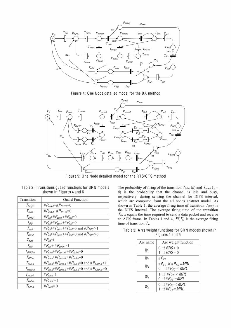
F igure 4: One Node detailed model for the B A method!

k

PDIFS1 Psense1 Pslot

Pbusy2

Psense2

PDIFS2

PBO

PtxRTSPFC

PrxRTS

PCTS

Pfail

TPG TDIFS1

Tidle1Tbusy1

Pbusy1TNAV1

TNAV2

TDIFS2Tbusy2

Tidle2

TBO

TRTS

Tsucc

Tfail

TCTS

Ttimeout

w2

w3

w4

w5

RNS

RNS

PACKTACK PtxDTtxD

PZRNS #PZRNS

TslotPBw1

TRNAV1

TNAV2

TRNAV2Tf1

Ts1

Tf2

Ts2

Pf1

Ps1

Ps2Pf2

!F igure 5: One Node detailed model for the R TS/C TS method

Table 2: T ransitions guard functions for SRN models

shown in F igures 4 and 6

Transition Guard Function Tbusy2 #Pbusy2+#PDIFS2=0 Tidle2 #Pbusy2+#PDIFS2=0 TDI FS #Pch+#Psucc +#Pfail=0 TBO #Pch+#Psucc +#Pfail=0 Tcoll #Pch+#Psucc +#Pfail=0 and #PFBO >1 TNcoll #Pch+#Psucc +#Pfail=0 and #PFBO >0 Tsucc #Pch=1 Tfail #Pch + #Pch-h > 1

TDI FS-h #Pch-h+#Psucc-h +#Pfail-h=0 TBO-h #Pch-h+#Psucc-h +#Pfail-h=0 Tcoll-h #Pch-h+#Psucc-h +#Pfail-h=0 and #PFBO-h >1 TNcoll-h #Pch-h+#Psucc-h +#Pfail-h=0 and #PFBO-h >0 Tsucc-h #Pch-h=1 Tfail-h #Pch-h > 1 TtxD-h #Psucc= 0

The probability of firing of the transition Tidle1 ( ) and Tbusy1 (1 ) is the probability that the channel is idle and busy,

respectively, during sensing the channel for DIFS interval, which are computed from the all nodes abstract model. As shown in Table 1, the average firing time of transition TDI FS1 is the DIFS interval. The average firing time of the transition TNAV1 equals the time required to send a data packet and receive an ACK frame. In Tables 1 and 4, F t(Tx) is the average firing time of transition Tx.

Table 3: A rcs weight functions for SRN models shown in

F igures 4 and 5

Arc name Arc weight function

W1 0 if RNS > 0 1 if RNS = 0

W2 #PFC

W3 #PFC if #PFC =MRL 0 if #PFC < MRL

W4 1 if #PFC < MRL 0 if #PFC =MRL

W5 0 if #PFC < MRL 1 if #PFC =MRL

The firing of transition Tidle1 deposits a random integer number of tokens in place Psense2 (start of backoff procedure), where the weight of arc between Tidle1 and Psense2 equals the random number RNS. RNS is uniformly distributed in the range [0, CW], where

CW = (CWmin + 1)

and the number of tokens in PFC (#PFC) represents the retry count to send a packet. The number of tokens in Psense2 represents the number of slots that the node has to wait before transmitting the packet. During any slot time, the channel may be busy, which is modelled by transition Tbusy2, or idle, which is modelled by transition Tidle2. If the channel became busy, the backoff timer is frozen for a time equals to the time of transmitting a data packet and receiving ACK frame. This is modelled by transition Tbusy2, place Pbusy2, and transition TNAV2. The end of frozen time is represented by firing of transition TNAV2 which deposits a token in PDI FS2. Sensing the channel for a DIFS interval before the backoff timer resumes decreasing is modelled by place PDI FS2 and transition TDI FS2. The probability that the channel is idle at the end of the current slot is represented by firing of transition Tidle2 which moves a token from Psense2 to Pslot. Firing of transition Tslot moves a token from Pslot to PBO which represents the decrement of the backoff timer by one slot.

The average firing time of the timed transition Tslot is Ts. The probability of firing of the transitions Tidle2 ( ) and Tbusy2 (1 ) are the probability that the channel is idle and busy, respectively, at the end of the current slot time, which are computed from all nodes abstract model. The average firing time of transition TDI FS2 and TNAV2 are equal to that of transition TDI FS1 and TNAV1, respectively .The guard function of the transition Tidle2, shown in Table 2, prevents the firing of the transition when there are any tokens in places Pbusy2 and PDIFS2 to prevent the decrement of the backoff timer when the channel is busy. The guard function of transition Tbusy2 and the inhibitor arcs between the place Pslot and transitions Tidle2 and Tbusy2 ensure that the processing of the next slot will not start before the end of the current slot (moving the token from Pslot to PBO).

Enabling and firing of transition TBO represents the end of the backoff. Because of the weight of arc between PBO and TBO, TBO is enabled if the number of tokens in PBO is greater than or equal RNS which means that the backoff timer reached zero. If the RNS is equal zero, the node has to transmit the MAC frame immediately without bakeoff delay. This means that the transition TBO must be enabled if the RNS is equal zero. So, the place PZRNS is added, where the transition Tidle1 deposits a token in it if RNS is equal zero. This is controlled by the arc weight function W1 shown in Table 3.

The firing of TBO deposits a token in PtxD and PFC which represents the start of transmitting the MAC frame by the physical layer and the retransmission retry counter, respectively. The end of transmitting the MAC frame is represented by the firing of TtxD that moves the token to PrxD which models the delivery of the MAC frame to the destination. If any other node starts to transmit any MAC frame at the same time, a collision occurs and transmission fails, otherwise, the frame is transmitted successfully. Therefore, the token in PrxD may move to Psucc due to firing of Tsucc, representing the success of transmitting the MAC frame, or move to Pfail due to firing of Tfail, representing the fail of transmitting the MAC frame

because of a collision. The average firing time of the transition TtxD is the transmission time of MPDU, the transmission time of the physical header (PhH), and the propagation time (Tp), as shown in Table 1. The probability of firing of Tsucc ( ) and Tfail (1 ) are computed from all nodes abstract model.

If the destination received the data frame successfully (the token in Psucc), it sends the ACK frame after SIFS interval which is represented by firing TACK. Transition TACK flushes the place PFC, which models the resetting the backoff counter to zero, and deposits a token in PB which lets a new packet to be transmitted. The firing of transition Ttimeout models an ACK timeout. Depending on the number of tokens in PFC, transition Ttimeout may deposit a token in PB or PDIFS1. If #PFC is less than the maximum retry limit (MRL), Ttimeout deposits a token in PDIFS1

PF C. Otherwise it deposits a token to PB and flushes PFC which models dropping the packet after reaching the maximum retry limit. This is controlled by the arcs weight functions w2, w4, and w5, as shown in Table 3.

As shown in Table 1, the average firing time of transition TACK is the transmission time of the ACK frame, the transmission time of the physical header, the propagation time, the time required to recognize the signal (CCA), the time required to convert from receiving to transmitting state (TRxTx), and SIFS interval. The average firing time of transition Ttimeout is the time required to send a data packet and receive an ACK frame, so it is equal to the average firing time of transitions TtxD (F t(T txD)) and TACK (F t(TACK)).

Table 4: The average fir ing time of timed transitions of

SRN models shown in F igures 5 and 7

Transition Average firing time TPG

TDIFS1, TDI FS2 DIFS TNAV1, TNAV2 F t(TRTS) + F t(TCTS ) + F t(TtxD ) + F t(TACK)

TRNAV1, TRNAV2 F t(TCTS)+ 2SIFS+2ts Tslot Ts TBO As Ts

TRTS

TCTS

TtxD

TACK

Ttimeout F t(TRTS ) + F t(TCTS)

5.2 One Node Detailed Model for R TS/C TS Method

Figure 5 shows the SRN model of the one node detailed model for the RTS/CTS method. Compared with the one node model for the BA method, the one node model of RTS/CTS method has a few differences. The token in Pbusy1 represents that the channel is busy and the node has to wait till the end of ongoing transmission from any other node. If the current transmission sent the RTS and CTS frames successfully, the NAV of the node is set and it has to wait until the end of transmitting the ACK frame (modelled by Ts1, Ps1, and TNAV1). Otherwise, the

channel will be sensed free for a period greater than 2 SIFS + tCTS + 2 Ts that let the node reset the NAV to zero and start again to sense the channel for DIFS interval (modelled by Tf1, Pf1, and TRNAV1). The probability of firing the conflicted transitions Ts1 ( ) and Tf1 (1 ) is the probability of success and failure to complete the RTS/CTS handshake, respectively, which are computed from all nodes abstract model. The average firing time of the timed transition TNAV1 is equal to the time needed to complete the RTS/CTS handshake. The average firing time of TRNAV1 is 2 SIFS + tCTS + 2 Ts.

The token in Pbusy2 represents that the channel is busy and the backoff timer stopped till the end of the ongoing transmission. The function of transitions Ts2, Tf2, Ps2, Pf2, TNAV2, and TRNAV2 are the same as Ts1, Tf1, Ps1, Pf1, TNAV1, and TRNAV1, respectively, but with backoff procedure. Also the average firing time and probability of the corresponding transitions are the same, as shown in Table 4. PtxRTS, TRTS, and PrxRTS model the transmitting the RTS frame by the source and receiving it by the destination. The average firing time of TRTS equals the transmission and propagation time of the RTS frame. If the destination received the RTS frame without any errors, Tsucc fires depositing a token in PCTS, otherwise Tfail fires. PCTS and TCTS represent transmission of the CTS frame. Receiving of the CTS frame and transmitting of data packet are represented by PtxD and TtxD. The destination sends the ACK frame after receiving the data packet and this is represented by PACK and TACK. Firing of transition Ttimeout models CTS frame timeout. The average firing time of the transition TCTS, TtxD, TAC K, and Ttimeout are shown in Table 4.

!F igure 6: The all nodes abst ract model for the B A method

5.3 Abstract Model for the B A and R TS/C TS Method

Figure 6 shows the all nodes abstract model for the BA method. It consists of two parts with a similar structure, the active and hidden part. The active and hidden parts represent the abstracted model for the nodes in active and hidden areas, respectively. The arcs between the active and hidden parts illustrate the interaction between the nodes in the active and hidden areas. To drive an abstracted model, for the nodes in either the active or hidden area, the backoff procedure and retry count in the one node detailed model are folded. Then, to exploit the identical

behaviour of all nodes, the models of all nodes in the same area are combined together using the lumping technique. The meaning of the places and transitions are explained below.

The a packet to transmit is represented by the number of tokens in PB. Transition TPG models the generation of packets from upper layer. The place PDIFS1 represents that the node is sensing the channel for a DIFS period. If the channel is free for the DIFS interval, transition TDI FS fires moving a token from PDI FS to PBO. The state of the channel is represented by the place Pch. If the number of tokens in Pch is zero, the channel is idle. Otherwise the channel is busy. As shown in Table 2, Transition TDI FS is assigned a guard that disable it if the channel is busy (#Pch > 0).

The number of tokens in PBO represents the number of nodes in backoff state. The firing of transition TBO represents the end of backoff procedure for all nodes that entered the backoff state (moving all tokens from PBO to PFBO). A guard is assigned to transition TBO to prevent its firing if the channel is busy. The average firing time of TBO is As Ts, where As is the average number of slots computed from the one node detailed model. The tokens in PFBO enable the conflicted transitions Tcoll and TNcoll. Transition Tcoll represents the probability that the backoff timer of two or more nodes reached zero at the same time making packets collide, whereas the probability of no collision is represented by TNcoll. If the channel is busy, the guards of Tcoll and TNcoll disable them. The collision probability increases with increasing of #PBO and decreasing of As. So, the firing probability of Tcoll and TNcoll depends on #PFBO and As, as shown in Table 5.

Table 5: The fir ing probability of immediate transitions of

SRN models shown in F igures 6 and 7

Transition Firing Probability

Tcoll

TNcoll

Tcoll-h

TNcoll-h

The firing of Tcoll moves all tokens in PFBO to PtxD and Pch, while firing of TNcoll moves one token from PFBO to PtxD and Pch. Places PtxD and PrxD and transition TtxD present the transmission and receiving of the data packet. Depending on the number of tokens in Pch either the immediate transition Tsucc or Tfail are enabled. If the number of tokens in Pch equals one (only one node uses the channel), the transition Tsucc is enabled, otherwise Tfail is enabled. Firing of transition Tsucc deposits a token in Psucc representing the success of receiving the data packets. Transmitting the ACK frame is represented by TACK. Tokens in Pfail represent the failure of the destination to receive the data packet. The ACK frame timeout is modelled by the transition Ttimeout. To make a synchronization between collided packets, the same number of tokens moves from PFBO to PDI FS through Tcoll, PtxD, TtxD, PrxD, Tfail, Pfail, and Ttimeout. This is controlled by the arc weight functions w4, w5, w6, w7, w8, w10, shown in Table 6.

Table 6: A rcs weight functions for SRN model shown in

F igures 6

Arc name Arc weight function

W1 #PBO if #Pch=0 and #PBO >0 1 if #PBO=0

W2 #PBO

W3 #PBO if #PFBO >1 1 if #PFBO=0

W4 #PFBO W5 #PFBO

W6 #PtxD if #PtxD > 0 1 if #PtxD=0

W7 #PtxD W8 #PrxD

W9 #Pch if #Pch > 0 0 if #Pch=0

W10 #PrxD

W11 #Pfail if #Pfail > 0 1 if #Pfail=0

W12 #Pfail

!F igure 7: The all nodes abst ract model for R TS/C TS

method

As shown in Figure 6, the structures of the abstracted SRN model for nodes in active and hidden area are similar. The place Px-h, transition Tx-h, and arc weight function hx correspond to Px, Tx, and wx, respectively, where x is the name of the identifier (place, transition, or the arc weight function). The meaning and function of all corresponding identifiers are the same.

If a node S in active area is transmitting a data packet to a destination D that overlapped with a transmission of another data packet in hidden area, the collision occurs at the destination D. So, the inhibitor arc between Pch-h and Tsucc is added to disable Tsucc and enable Tfail when the number of token in Pch-h is greater than zero. If the destination D received the data packet successfully, it will send the ACK frame. During

sending the ACK frame the hidden nodes sense the channel busy which make them stop sensing the channel for DIFS interval and stop the backoff counter. This is represented by the inhibitor arcs from Psucc to transitions TDI FS-h and TBO-h.

The all nodes abstract model for the RTS/CTS method is shown in Figure 7. Compared to the corresponding SRN model for the BA method, shown in Figure 6, there are a few differences. Places PtxRTS and PrxRTS and transition TtxRTS represent the transmitting and receiving of an RTS frame. Receiving of an RTS frame, transmitting of a CTS frame and receiving of a CTS frame are modelled by PCTS, TCTS, and PtxD, respectively. If the source received the CTS frame, it transmits the data packet. When the destination receives the data packet successfully, it sends the ACK frame. This is modelled by places PtxD and PACK, and transitions TtxD and TACK. As shown in Table 4, the average firing time of transitions TRST, TCTS, TtxD, and ACK are the transmission, sensing and interframe spacing time of RTS, CTS, data, and ACK frames, respectively. The arcs weight functions are shown in Table 7. Also, the structure of the abstracted SRN model for the nodes in hidden area is similar to that of the nodes in active area. The place Px-h, the transition Tx-h, and the arc weight function hx correspond to Px, Tx, and wx, respectively, where x is the name of the identifier. The meaning and function of all corresponding identifiers are the same.

Table 7: A rcs weight functions for SRN model shown in

F igure 7

Arc name Arc weight function

W1 #PBO if #Pch=0 and #PBO >0 1 if #PBO=0

W2 #PBO

W3 #PBO if #PFBO >1 1 if #PFBO=0

W4 #PFBO W5 #PFBO

W6 #PtxRTS if #PtxRTS > 0 1 if #PtxRTS=0

W7 #PtxRTS W8 #PrxRTS

W9 #Pch if #Pch > 0 0 if #Pch=0

W10 #PrxRTS

W11 #Pfail if #Pfail > 0 1 if #Pfail=0

W12 #Pfail

For RTS/CTS method, there are many interactions between the nodes in active area and hidden nodes compared to BA method. In Figure 3, if the hidden node Sh1 sent a RTS frame to the destination Dh1, the destination D1 of the source node S1will receive it. Consequently, D1 sets its NAV to a value that prevents it from sending any CTS or ACK frames until Sh1 receives the ACK frame from Dh1. Therefore, if D1 received a RTS frame from S1 S1which produces a timeout error for the RTS frame. This is modelled by adding inhibitor arcs from places PCTS-h, PtxD-h, and PACK-h to the transition Tsucc, as shown in Figure 7. In addition, if the nodes Sh1 and S1 sent a RTS frame at the same time, the collision occurs at the destination D1 that also produces a

timeout error. So, we added the inhibitor arc between the place Pch-h and transition Tsucc which disables it and enables Tfail. When any destination in active area (e.g D1) sends a CTS frame to the source (e.g. S1), the hidden nodes will receive it, thus they stop all activities until the destination receives the data packet and sends the ACK frame. We figured this situation by adding inhibitor arcs between transitions TDI FS-h and TBO-h and places PtxD and PACK, as depicted in Figure 7.!

In order to solve the proposed model analytically, we modelled all events in IEEE 802.11 DCF MAC protocol using exponentially distributed timed transitions although some of these events, such as DIFS interval, backoff slot time, and packets transmission time, are deterministic in reality. In Section 6, the proposed models will be validated by comparison with detailed simulations. Compared to simulation results, the proposed models provide accurate results under different system parameters.

Table 8: T ransitions guard functions for SRN models

shown in F igures 5 and 7

Transition Guard Function Tbusy2 #Pbusy2+#Ps2+#Pf2+#PDIFS2=0 Tidle2 #Pbusy2+#Ps2+#Pf2+#PDIFS2=0 TDI FS #Pch+#PCTS +#PtxD +#PACK +#Pfail=0 TBO #Pch+#PCTS +#PtxD +#PACK +#Pfail=0 Tcoll #Pch+#PCTS +#PtxD +#PACK +#Pfail=0 and #PFBO >1 TNcoll #Pch+#PCTS +#PtxD +#PACK +#Pfail=0 and #PFBO >0 Tsucc #Pch=1 Tfail #Pch +#Pch-h+#PCTS-h+#PtxD-h+#PACK-h > 1

TDI FS-h #Pch-h+#PCTS-h+#PtxD-h+#PACK-h+#Pfail-h +#PCTS= 0 TBO-h #Pch-h+#PCTS-h +#PtxD-h+#PACK-h+#Pfail-h+#PCTS =0

Tcoll-h #Pch-h+#PCTS-h+#PtxD-h+#PACK-h+#Pfail-h=0 and #PFBO >1

TNcoll-h #Pch-h+#PCTS-h +#PtxD-h+#PACK-h+#Pfail-h=0 and #PFBO >0

Tsucc-h #Pch-h=1 Tfail-h #Pch-h > 1 TRTS-h #PCTS +#PtxD +#PACK =0 TtxD-h #PtxD + #PACK=0

5.4 The Analytical Procedure

For the BA and RTS/CTS methods, the one node detailed model is used to drive the average size of backoff window (As) which is exported to the all nodes abstract model. The average number of tokens in the place Pslot represents the average size of backoff window. The all nodes abstract model is used to drive the performance metric and the parameters , , and . These parameters are computed using the following equations

=Pr ( #PDIFS1 > 0 & #Pch > 0) =Pr ( #PBO > 0 & #Pch > 0) =Pr ( #Pch=1 & #Pch-h >= 0)

where Pr(E) is the probability of the event E. The computed parameters , , and are used to solve the one node detailed model. According to the following procedure, the two models

are solved iteratively until the convergence of the performance metrics:

Step 1- The initial value of the average size of backoff window is computed using the following equation:

Step 2- Solve the all nodes abstract model using the initial value of backoff window and get the initial values of a performance metric (e.g. throughput) and parameters , , and .

Step 3- Solve the one node detailed model using the last computed values of parameters , , and and get the new value for As.

Step 4- Solve the all nodes abstract model and get the performance metric n and parameters , , and , where n is the number of iteration.

Step 5- Compute the error using the following equation err( )=| n n 1 | / n

Step 6- If the err( ) is less than a specified threshold, stop the iteration process, otherwise increase n by one and go to Step 3.

In all validation scenarios introduced in the validation section the convergence of the performance metric is achieved in only a few iterations.

Table 9: M A C and Physical layer Parameters

Parameter Value CWmin 31 CWmax 1023 ts 20 TRxTx 5 TCCA 15 DIFS 50 SIFS 10 PhH 192 bit MAC Header 292 bit RTS 160 bit + PhH CTS 112 bit + PhH ACK 112 bit + PhH B1 1 Mbps B2 2 Mbps SRC 6 LRC 4

6. M O D E L V A L ID A T I O N

In this section, we examine the accuracy of the proposed SRN models for both the BA and RTS/CTS methods by making extensive comparisons of their results with the results of simulation experiments. The simulation results were obtained by using the ns2 simulator [24]. The ns2 simulator is one of the most powerful tools for extracting accurate performance indices for wireless networks. According to the IEEE 802.11 standard [7], Table 9 shows the parameters of physical and MAC layer used in the simulation and analysis. For each node, the transmission and carrier sensing range are 250 and 550m,

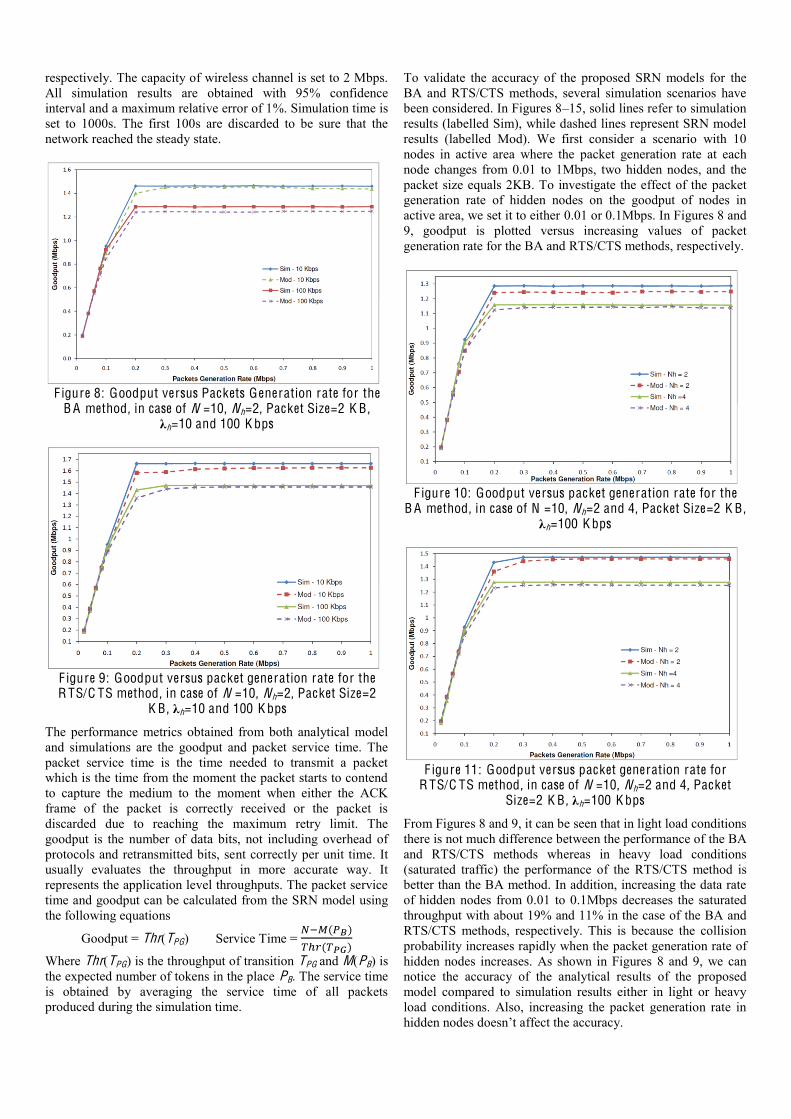
respectively. The capacity of wireless channel is set to 2 Mbps. All simulation results are obtained with 95% confidence interval and a maximum relative error of 1%. Simulation time is set to 1000s. The first 100s are discarded to be sure that the network reached the steady state.

F igure 8: Goodput versus Packets Generation rate for the

B A method, in case of N =10, Nh=2, Packet Size=2 K B , h=10 and 100 K bps

F igure 9: Goodput versus packet generation rate for the

R TS/C TS method, in case of N =10, Nh=2, Packet Size=2

K B , h=10 and 100 K bps

The performance metrics obtained from both analytical model and simulations are the goodput and packet service time. The packet service time is the time needed to transmit a packet which is the time from the moment the packet starts to contend to capture the medium to the moment when either the ACK frame of the packet is correctly received or the packet is discarded due to reaching the maximum retry limit. The goodput is the number of data bits, not including overhead of protocols and retransmitted bits, sent correctly per unit time. It usually evaluates the throughput in more accurate way. It represents the application level throughputs. The packet service time and goodput can be calculated from the SRN model using the following equations

Goodput = Thr(TPG) Service Time =

Where Thr(TPG) is the throughput of transition TPG and M(PB) is the expected number of tokens in the place PB. The service time is obtained by averaging the service time of all packets produced during the simulation time.

To validate the accuracy of the proposed SRN models for the BA and RTS/CTS methods, several simulation scenarios have been considered. In Figures 8 15, solid lines refer to simulation results (labelled Sim), while dashed lines represent SRN model results (labelled Mod). We first consider a scenario with 10 nodes in active area where the packet generation rate at each node changes from 0.01 to 1Mbps, two hidden nodes, and the packet size equals 2KB. To investigate the effect of the packet generation rate of hidden nodes on the goodput of nodes in active area, we set it to either 0.01 or 0.1Mbps. In Figures 8 and 9, goodput is plotted versus increasing values of packet generation rate for the BA and RTS/CTS methods, respectively.

F igure 10: Goodput versus packet generation rate for the

B A method, in case of N =10, Nh=2 and 4, Packet Size=2 K B , h=100 K bps

F igure 11: Goodput versus packet generation rate for

R TS/C TS method, in case of N =10, Nh=2 and 4, Packet

Size=2 K B , h=100 K bps

From Figures 8 and 9, it can be seen that in light load conditions there is not much difference between the performance of the BA and RTS/CTS methods whereas in heavy load conditions (saturated traffic) the performance of the RTS/CTS method is better than the BA method. In addition, increasing the data rate of hidden nodes from 0.01 to 0.1Mbps decreases the saturated throughput with about 19% and 11% in the case of the BA and RTS/CTS methods, respectively. This is because the collision probability increases rapidly when the packet generation rate of hidden nodes increases. As shown in Figures 8 and 9, we can notice the accuracy of the analytical results of the proposed model compared to simulation results either in light or heavy load conditions. Also, increasing the packet generation rate in

To illustrate the influence of the number of hidden nodes on the goodput of the nodes in active area, in Figures 10 and 11 we plot the goodput versus the packet generation rate at nodes in active area, in the case of the BA and RTS/CTS methods, where N=10, Nh=2 or 4, h=0.1Mbps, and the packet size is 2KB. The figures show that, for either the BA or RTS/CTS methods, in high traffic load the goodput deteriorates when the number of hidden nodes increases due to increasing of interference and collision probability. In addition, the accuracy of the results of the proposed models was not affected by the number of hidden nodes.

F igure 12: Saturated goodput versus number of nodes for

the B A method, in case of =2 M bps, Nh=2, Packet Size=2

K B , h=10 and 100 K bps

F igure 13: Saturated goodput versus number of nodes for

R TS/C TS method, in case of M bps, Nh=2, Packet Size=2

K B , h=10 and 100 K bps

Figures 12 and 13 show how the saturated goodput of nodes in active area is affected by varying the number of nodes in active area N from 6 to 20 for the BA and RTS/CTS methods, where Nh=2, h=0.01 or 0.1Mbps, =2Mbps, and the packet size is 2KB. It can be seen from Figure 12 that the performance of the BA method is strongly affected by the number of nodes in active area. It degrades with increasing number of nodes. On the contrary, Figure 13 shows that the performance of RTS/CTS method is nearly independent of the number of nodes. For the same scenario, in Figure 14, the packet service time is plotted versus the number of nodes in active area, which is varied from 6 to 20, for the BA and RTS/CTS methods. It is clear that the performance of the RTS/CTS method is better than the BA method, especially with large number of nodes. As shown in

Figures 13 and 14, the analytical results of the proposed model are close to the simulation results.

F igure 14: Packet service time versus number of nodes for

both the B A and R TS/C TS method, in case of =2 M bps, Nh=2, Packet Size=2 K B , h=10 K bps

F igure 15: Goodput versus packet generation rate for both

the B A and R TS/C TS method, in case of N =10, Nh=2, Packet Size=2 and 0.5 K B , h=10 K bps

In the last scenario, we investigate the effect of the packet size on the performance of the BA and RTS/CTS methods. We consider the case where the number of nodes in active area is fixed to 10 nodes, the number of hidden nodes is set to Nh=2, the packet generation rate at hidden nodes is set to 0.01 Mbps, and the packet size is set to 2KB or 0.5KB. The packet generation rate at nodes in active area is varied from 0.01 to 1Mbps. Figure 15 shows the goodput of nodes in active area versus the packet generation rate. From Figure 15, we can notice the following:

With light load conditions, the packet size has no significant effect on the performance of the network either in the case of the BA or RTS/CTS method. With heavy load conditions, the packet size strongly affects the performance of the network, where increasing the packet size from 0.5 to 2KB increased the goodput with about 20% and 37% in the case of the BA and RTS/CTS methods, respectively. The performance of the BA method is a little better than RTS/CTS method when the packet size is small.

For large packet size, the performance of RTS/CTS method is much better than the BA method. In all cases, the results of the proposed models are still accurate compared to simulation results.

7. C O N C L USI O NS

In this paper we have investigated the performance of the IEEE 802.11 DCF MAC protocol, for both the BA and RTS/CTS methods, in multi-hop ad hoc networks in the presence of hidden nodes using SRN models. The proposed models capture most features of the MAC protocol. The influences of system parameters, such as traffic load, packet size, and number of nodes, have been demonstrated.

The proposed SRN models for both the BA and RTS/CTS methods have been validated through extensive comparisons between analytical and simulation results. Comparisons showed that the proposed models succeeded to provide an accurate representation of the dynamic of the IEEE 802.11 DCF MAC protocol under several different settings of the system parameters.

Analytical results show that in light load condition there is not much difference between the performance of the BA and RTS/CTS methods. Conversely, in heavy load conditions the performance of RTS/CTS method is much better than the BA method. Also, the packet size, number of neighbour nodes, and number of hidden nodes have a great effect on the performance of ad hoc networks especially in the case of the BA method under saturated load conditions.

R E F E R E N C ES

[1] N. Abramson, The ALOHA system - another alternative for computer communications, in: Proceedings of the AFIPS Conference, pp. 295-298, 1970.

[2] L.G. Roberts, ALOHA packet system with and without slots and capture, Computer Communications Review, 1975.

[3] L.K.a.F.A. Tobagi, Packet switching in radio channels: Part I carrier sense multiple-access modes and their throughput-delay characteristics, IEEE Transactions on Communications, pp. 1400 1416, 1975.

[4] P. Karn, MACA - a new channel access method for packet radio, in: Proceedings of the 9th ARRL Computer Networking Conference, pp. 134 140, 1990.

[5] A.D.V. Bharghavan, S. Shenker, and L. Zhang, MACAW:

Proceedings of ACM SIGCOMM, pp. 221 225, 1994. [6] L.F. Chane, and J.J. Garcia-Luna-Aceves, Floor acquisition

multiple access (FAMA) for packet-radio networks, in: Proceedings of the Conference on Applications, technologies, architectures, and protocols for computer communication, ACM, 1995.

[7] Wireless LAN Medium Access Control (MAC) and Physical Layer (PHY) Specifications, IEEE standards 802.11, 1999-2007.

[8] R. Jain, The Art of Computer Systems Performance Analysis: Techniques for Experimental Design, Measurement, Simulation, and Modelling, New York: John Wiley & Sons, 1991.

[9] G. Bianchi, Performance analysis of the IEEE 802.11 distributed coordination function, IEEE Journal on Selected Areas in Communications, 18(3), pp. 535-547, 2000.

[10] H. Wu, Y. Peng, K. Long et al, Performance of reliable transport protocol over IEEE 802.11 wireless LAN: Analysis and enhancement, in: Proceedings - IEEE INF OCOM, pp. 599-607, 2002.

[11] E. Ziouva, and T. Antonakopoulos, CSMA/CA performance under high traffic conditions: Throughput and delay analysis, Computer Communications, 25(3), pp. 313-321, 2002.

[12] C.H. Foh, and J.W. Tantra, Comments on IEEE 802.11 saturation throughput analysis with freezing of backoff counters, IEEE Communications Letters, 9(2), pp. 130-132, 2005.

[13] F. Eshghi, and A.K. Elhakeem, Performance analysis of ad hoc wireless LANs for real-time traffic, IEEE Journal on Selected Areas in Communications, 21(2), pp. 204-215, 2003.

[14] E. Ziouva, and T. Antonakopoulos, The IEEE 802.11 Distributed Coordination Function in Small-Scale Ad-Hoc Wireless LANs, International Journal of Wireless Information Networks, 10(1), pp. 1-15, 2003.

[15] O. Tickoo, and B. Sikdar, Queueing analysis and delay mitigation in IEEE 802.11 random access MAC based wireless networks, in: Proceedings of IEEE INF OCOM, pp. 1404-1413, 2004.

[16] T.C. Hou, L.F. Tsao, and H.C. Liu, Throughput Analysis of the IEEE 802.11 DCF Scheme in Multi-hop Ad Hoc Networks, in: Proceedings of the International Conference on Wireless Networks, pp. 653-659, 2003.

[17] H. Ting-Chao, T. Ling-Fan, and L. Hsin-Chiao, Analyzing the throughput of IEEE 802.11 DCF scheme with hidden nodes, in: Proceedings of the 58th Vehicular Technology Conference, Vol.5, pp. 2870-2874, 2003.

[18] Y. Wang, and J.J. Garcia-Luna-Aceves, Modeling of collision avoidance protocols in single-channel multi-hop wireless networks, Wireless Networks, 10(5), pp. 495-506, 2004.

[19] O. Ekici, and A. Yongacoglu, IEEE 802.11a throughput performance with hidden nodes, IEEE Communications Letters, 12(6), pp. 465-467, 2008.

[20] R. German, and A. Heindl, Performance evaluation of IEEE 802.11 wireless LANs with stochastic Petri nets, in: Proceedings of the 8th International Workshop on Petri Nets and Performance Models, pp. 44-53, 1999.

[21] R. Jayaparvathy, S. Anand, S. Dharmaraja et al, Performance analysis of IEEE 802.11 DCF with stochastic reward nets, International Journal of Communication Systems, 3, pp. 273-296, 2007.

[22] G. B. M.A. Marsan, G. Gonte, , S. Donatelli, and G. Franceschinis, Modeling With Generalised Stochastic Petri Nets, John Wiley & Sons, 1995.

[23] K. Xu, M. Gerla, and S. Bae, Effectiveness of RTS/CTS handshake in IEEE 802.11 based ad hoc networks, Ad Hoc Networks, 1(1), pp. 107-123, 2003.

[24] The Network Simulator ns-2 v2.34, available at http://www.isi.edu/nsnam/ns/.

!