THE UNIVERSITY OF MICHIGANPROGRAM IN SHIP HYDRODYNAMICS

COLLEGE OF ENGINEERING

NAVAL ARCHITECTURE &MARINE ENGINEERING

AEROSPACE ENGINEERING

MECHANICAL ENGINEERING &APPLIED MECHANICS

SHIP HYDRODYNAMIC

SS I \ LABORATORY

5 S5SS~ 5SPACE PHYSICS RESEARCH

( LnBORATORY5 i ikh

II AD-A251 101

ICollision of a Vortex Pair

* with a Contaminated Free Surface

Gr6tar Tryggvason and Javad Abdollahi-AlibeikDepartment of Mechanical Engineering and Applied Mechanics

U William W. Willmarth and Amir HirsaDepartment of Aerospace Engineering D TICContract Number NOOO -86-K-0684 , " T

Technical Report No. 90-1 JUN 1992

October, 1990

,_ Appr-'. L. d f pi,,> s .-

.'-D'st ut!on Unlmni ted

IIIIIII

I 92-137989 \UUUII UU544

I

I Collision of a vortex pair with a contaminated free surface

Griar Trjggvajon

Javad AbdollaJi-Alibeik

William W. Willmarth

Amir Hirsa

The University of MichiganAnn Arbor, MI 48109

Abstract

Collision of a viscous vortex pair with a free, contaminated surface is studiednumerically. The Froude number is assumed to be small so the surface remainsflat. The full Navier-Stokes equations and a conservation equation for the surfacecontaminant are solved numerically by a finite difference method. The shear stressat the free surface is proportional to the contamination gradient, and simulations forseveral values of the proportionality constant (W), as well as Reynolds numbers,have been performed. The evolution is also compared with full-slip and no-slipboundaries. As the vortices approach the surface, the upwelling between thempushes the contaminant outward, reducing the amount directly above the vortices,and leading to a clean region for low W, as well as for a full-slip boundaries. AsW is increased the clean region becomes smaller, and eventually no clean regionis formed. Except for very low W, the contaminant layer leads to the creationof secondary vortices, causing the original vortices to rebound in a similar way asvortices colliding with a no-slip boundary. For one case, the numerical results arecompared with experimental measurements with satisfactory results. Computationsof a vortex pair colliding obliquely with a contaminated surface and head-on collisionof axisymmetric vortex rings are also presented.

URI Report 90-1

To be submitted for publication in 1990

Statement A per telecon Dr. Edwin RoodONR/Code 1132 4". ! ' rArlington, VA 22217-5000 . .

NWW 6/1/92 _ ________./

I 4,04 9 wl

I % A"' !2 b ! ' i *.FCodes

Dlz i:- Spacial

1. Introduction

For fluid mechanics problems involving a free surface, it is often important to

account for surface tension effects, particularly for small scale phenomena. The in-

clusion of a finite surface tension generally leads to technical complications in both

numerical and analytical work. However, even when surface tension is properly

accounted for, the results may not account correctly for observations. The reason

is, usually, that most fluids are not completely clean, and ever a small amount of

contaminant can alter the surface tension of a free surface considerably. Modifica-

tion of waves by the addition of a contaminant and the difference in rise velocity

of air bubbles in clean and contaminated water are well-known examples. A simple

I change in surface tension is, by itself, not a major problem. Rather, the surface

flows leads to a nonuniform spatial distribution of contaminants, which, in turn,

I causes variable surface tension. This nonuniform surface tension can induce surface

motion that may alter the flow characteristics considerably. In this paper we study

I numerically the modification of a simple, unsteady, vortical flow by a contaminated

surface.

I The evolution of a vortical flow near a free surface and the resulting surface

deformations have recently been the subject of several investigations motivated pri-

marily by a desire to understand the surface signature of ship wakes. Sarpkaya

(1986) towed a small delta wing below a free surface, keeping the wing at a neg-

ative angle of attack so that the trailing vortices ascended to the free surface. As

the vortices approached the surface, Sarpkaya observed two distinct types of surface

signatures. First, before the vortices collide with the surface, relatively irregular

and three-dimensional "striations" appear, consisting of streaks perpendicular to

the line of motion. These are followed by a pair of long and narrow marks parallel

to the line of motion and outboard of the wing. These "scars" appear to be directly

I related to the trailing vortices, and move outward with the vortices. A somewhat

different setup, consisting of a two-dimensional vortex pair was studied by Will-

I marth, Tryggvason, Hirsa and Yu (1989) and by Sarpkaya, Elnitsky II, and Leeker

Jr. (1989). The surface signature of the pairs is similar to the trailing vortices,

I but the mean motion is now strictly two-dimensional. More complicated flows were

studied by Bernal and Madnia (1989) who investigated the generation of surface

1j 2

LI

I

I waves due to a jet below a free surface and showed that the "opening up" of vortex

rings at the surface generates considerable amount of small scale surface waves. To

iUi. explore this mechanism in more detail, Bernal and Kwon (1989) experimented with

a single ring colliding obliquely with the surface. More recently, Song, Bernal, and

I Tryggvason (1990) have experimented with large vortex rings colliding head on with

a free surface.

II Several numerical studies of this problem have paralleled the experimental work.

Tryggvason (1988) presents a brief numerical study of surface deformation due to the

roll-up of a submerged vortex sheet using a boundary integral/vortex method, and

Willmarth et al (1989) simulated the formation of a vortex pair from an initially

flat vortex sheet and the subsequent vortex and free surface motion. They also

made a brief comparison of experimental and computational results. Sarpkaya,

Elnitsky II, and Leeker Jr. (1989) and Telste (1989) also used a boundary integral

technique to follow the motion of a point vortex pair toward a free surface. A finite

Idifference simulation of the point vortex problem has been reported by Marcus

and Berger (1989), who also discuss linearized aspects of the problem. A thorough

11 discussion of both vortex collision as well as the formation of vortices from a shear

layer and the resulting surface signature, is given by Yu and Tryggvason (1990), who

simulated a large number of cases and, in particular, explored the limits of high and

low Froude numbers. These computations all assume an inviscid, two-dimensional

stI! motion. Axisymmetric calculations are contained in Song, Bernal, and Tryggvason

(1990) along with experimental results.

Ii1 The above experimental and numerical investigations were not concerned with

the effects of surface contaminants as such, but it appears that some of the ex-

perimental results were influenced by the fact that a free surface is hardly ever

completely clean. Earlier, Davies (1966) discussed the damping of turbulent eddies

at a free surface (and reviewed earlier work), and Davies and Driscoll (1974) experi-

mented with ejecting pulses of colored water to a free surface, specifically addressing

the rate of surface renewal and the effect of contamination on the free surface. Theyfound that the spreading of the colored water at the surface is reduced considerably

for contaminated surfaces. However, their primitive visualization technique did not

allow for a clear explanation of the mechanism responsible for this behavior. Ex-

*1 31. __ __ _

I periments on the collision of two-dimensional vortex pairs with a free, as well as

rigid, surface were reported by Barker and Crow (1977). The motivation for their

I experiments was the observed rebounding of aircraft trailing vortices from rigid

(no-slip) surfaces (see e.g. Harvey and Perry, 1971). This rebounding of a vortex

I pair from a solid surface is due to the separation of the ground boundary layer and

the subsequent formation of secondary vortices and is therefore not expected if the

I rigid surface is replaced by a stress-free free surface. However, Barker and Crow

(1977) observed rebounding in their free surface experiments, just as for a rigid

I surface, and suggested that this rebounding might be due to inviscid effects such

as the deformations of the vortex cores. Saffman (1979) refuted this suggestion,

I and showed that for inviscid flow and a flat boundary, rebounding cannot occur

and suggested that the behavior might be due to contamination effects. Peace and3 IRiley (1983) performed numerical simulations of the full Navier-Stokes equations

for a plane vortex pair colliding with a flat no-slip and a stress-free surface and3 Iargued that even for stress-free boundaries, viscosity could cause rebounding. How-

ever, even though their calculations clearly show rebounding, those are for a rather

low Reynolds numbers. With an increasing Reynolds number, the rebounding de-

creased significantly. Their argument can therefore not explain the behavior in the

Barker and Crow experiment, which was conducted at a much higher Reynolds

number. Recent computations by Orlandi (1990) (as well as those in this paper)

show, indeed, that at high enough Re no rebounding takes place for a stress-free

boundary.

I The explanation for rebounding from a free surface is clear from recent exper-

iments by Bernal, Hirsa, Kwon, and Willmarth (1989) and Willmarth and Hirsa

(1990), who investigated the collision of both vortex rings and planar vortex pairs

with a free surface. They observe (as Driscoll and Davis) that the cleanness of the

surface influences considerably the vortex motion itself. For a very clean surface,

sufficiently weak vortices are deflected outward, in a manner similar to what inviscid

theory predicts (if the surface deforms, some rebounding is predicted, but most of

the experiments have been performed under conditions where surface deformation

is minimal), but for a contaminated surface, the behavior was more like vortices en-

countering a rigid wall. Secondary vorticity from the wall boundary layer is pulledI4

I

I away by the primary vortex that then rebounds as a result of its interaction with

the wall vorticity. Detailed observation by LIF (Laser Induced Fluorescence) lead

I Bernal et. al. to conclude that the surface motion induced by the vortex generates

an uneven distribution of surface contaminant that, in turn, caused a shear at the

surface. The shear generates vorticity that the primary vortex sweeps into the inte-

rior, eventually leading to the rebounding of the primary vortex. This injection of

vorticity and its subsequent interaction with the primary vorticity appears to be the

leading effect of the surface contaminants. Detailed measurements of the velocity

3 field for a vortex pair as well as observations of the contaminant distribution on the

surface for various amounts of contaminant are presented by Willmarth and Hirsa

t(1990).

Observations of contaminated surfaces have been reported on numerous occa-

sions for more than a century. One of the more common phenomena is the so-called

Reynolds ridge, which appears on the boundary between contaminated and clean

surface when the contaminated region is compressed by an inflow of clean water.

This is precisely the case wben vortices collide with a free surface as in the exper-

I iments of Willmarth and Hirsa (1990). The upwelling generated by the vortices

pushes the contaminated surface water to the side, thereby compressing the con-

I tamination layer. The surface above the vortices is clean and is separated from the

contaminated surface by a Reynolds ridge. We should note that the occurrence of a

3 Reynolds ridge, although often observed when separation takes place, is not directly

related to the generation of secondary vortices. Indeed, a Reynolds ridge is easily

generated in the absence of separation (see e.g. Scott, 1982), and separation can

take place without the formation of a Reynolds ridge. For a thorough discussion of

the Reynolds ridge with historical perspective see Scott (1982). In the calculations

presented here, the surface is assumed to remain flat, so, strictly speaking, no ridge

can appear. However, the clean and contaminated surface is often separated by a

sharp boundary, and it appears that the vorticity beneath the contaminated surface

outboard of this sharp boundary-not the small ridge elevation-is what influences

the flow evolution.

I The modification of flows with a free surface is of considerable importance in a

number of other problems. We mention specifically bubble flow, where contarnina-I

I

lI tion sometimes reduces the velocity of a rising buoyant bubble. This effect has been

reviewed by Harper (1972), and recent boundary integral calculations of bubbles in

I an axisymmetric strain field have been conducted by Stone and Leal (1989). Flows

due to surface tension variations induced by a changing temperature, the Marangoni

I effect, have been studied on several occasions (see e.g. Ostrach, 1982).

Although rebounding can usually be associated with viscous effects, Dahm,

Schiel, and Tryggvason (1989) have shown that a weak vortex colliding with a weak

Sdensity interface can pull up a portion of the interface containing baroclinically

generated vorticity that then causes the primary vortex to rebound in completely

inviscid simulations. Yu and Tryggva.son (1990) also show that a deformable surfacecan lead to inviscid rebounding. However, this occurs at much higher Froude num-

bers than in the experiments of Willmarth and Hirsa (1990). Recent calculations

by Ohring and Lught (1990) show that rebounding in viscous fluids at much higher

Froude numbers can take place due to secondary vorticity created by large surface

curvature.

In this paper, we investigate the modification of a vortical flow due to the pres-

ence of a contaminant on a free surface. The calculations complement the ex-

periments of Willmarth and Hirsa (1990), and we compare some of our results to

theirs. The fluid is assumed to be viscous, and the full Navier-Stokes equations are

solved numerically. Although inviscid methods can easily be modified to account for

constant surface tension and can easily predict the redistribution of a surface con-

taminant, the resulting shear stress is incompatible with the inviscid model. Since

we are only concerned with low Froude number flows where surface deformations

are small, we assume a flat surface. Three-dimensional effects are also assumed to

be absent. Preliminary results from similar calculations, but with a more limited

scope, have been presented by Wang and Leighton (1990).

In section 2 we discuss the mathematical model, the numerical method, and

the relevant dimensionless parameters. The method is based on a straightforward,

second-order, finite difference approximation of the Navier Stokes equations in vor-

I ticity form; hence, we give only a brief description. In Section 3 we present our

results. First we discuss a number of calculations using a simple constitutive equa-I .I

Ution for the relation between the surface tension and the contamination and discuss

the influence of the relevant parameters, then we compare our results with the ex-

perimental study of Hirsa and Willmarth (1990), using a more realistic constitutive

equation. We conclude this section with a brief study of vortex rings colliding head3 on with the surface and vortex pairs colliding obliquely with the surface. Our con-

clusions appear in Section 4. A short account of some of the work reported here

was presented at the Eighteenth Symposium on Naval Hydrodynamics in August

1990, (see Hirsa, Tryggvason, Abdollai-Alibeik, and Willmarth, 1990).

i 2. Problem Formulation and Numerical Method

The flow is assumed to be viscous and confined to two dimensions. In addition to

two-dimensionality, the major limitation of our calculations is that the free surface

is assumed to remain flat for all times. This limits the results presented here to

low Froude numbers. However, this is the case that is most frequently studied

experimentally, and since the surface deformations are observed to be small, the

limitation is not as severe as one might think. In order to avoid any arbitrary

modeling of inflow and outflow boundaries, we simply take the boundary of the

domain to be full-slip walls except for the top. The effects of this limited domain

size iz ciscussed in the result section.

The flow is governed by the Navier-Stokes equation, which in vorticity form can

be written as an advection-diffusion equation for the vorticity

+ J(,w)= Re

U and a Poisson equation relating the stream function to the vorticity

V20 = -w. (2)

Here J(O,w) = (ft/e)(&1a/)- t01a/)(&w&/o), and the Reynolds number is

defined as Re = r/Y.

The equations have been nondimensionalized using the initial separation be-

tween the vortices and the initial circulation to construct a length and a time scale.

Time, velocity, and vorticity are therefore measured in units of L2/r, r/L, and

I r/L 2 , respectively. This gives a Froude number as VF/gL , which is assumed to

be small.

I

U

I The surface contaminant is assumed to be conserved, leading to a hyperbolic

conservation equationII Ci+ = 0, (3)

were u, is the horizontal velocity at the surface. Notice that since the surface

divergence of u. is in general not zero and depends on c, this equation allows for the

possibility of "contamination shocks" (that is the development of a discontinuity in

c). The surface contaminant affects the flow field through shear stresses induced by

variations in the surface tension, a. This induced shear is given by

ad (4)

Since the surface is fiat, the vorticity at the surface is w, = Ou/Oy. The surface

tension depends only on the amount of contaminant, a = a(c), and the boundary

condition for the vorticity, at the surface, is therefore

I = (5)

The quantity c.(da/dc) is usually called the elasticity of the surface. If the contam-

inant is nondimensionalized by its initial value, c., and the vorticity as before, we

end up with w. = W c/8: in nondimensional units, where

L dIW = F-CoT. (6)

The flow is governed by Re, W, and the initial vorticity configuration.

I In experiments, the viscosity of the liquid and the elasticity of the contaminant

are usually given, and the separation of the vortices may be difficult to change once

I the experimental apparatus has been built. A change in Reynolds number is thus

usually accomplished by an increase in the circulation, r, which, in turn, decreases

I w.In general, the elasticity of the surface depends strongly on both the composition

"[ • of the surface contaminant, as well as the amount of contaminant. For most of

the calculations reported here, we assume that the elasticity remains a constant.

The major reason for this simplification is our desire to focus on the most basic

aspect of the problem and to reduce the number of variable parameters as muchI

I

U as possible. For more complicated equations of state, additional parameters are

needed. The computational code is, however, not limited to this simple form, and

in our comparison with experiments, we have used the appropriate equation of state.

To solve equations (1)-(3) numerically, we use rather standard finite difference

approximations. Equation (1) is integrated by an explicit, second-order, predictor-

corrector method in time, and the spatial discretization is done with second-order

centered-differences. For the Jacobian, J(z, y), Arakaw's conservative stencil is

used. The Poisson equation, (2), is solved with a fast solver (HWCRT form FISH-

PAK). For (3) we also use a second-order predictor-corrector i, time, and second-

order differences in space. For stability, an artificial viscosity term is added on the

right hand side of (3). This term is small everywhere except where the contaminant

value changes rapidly. The surface velocity is found by a one-sided, second-order

differentiation of the stream function. Several of our results have been checked for

convergence by repeating the calculation using a different resolution.

3. Results

3.1 Parameter Studies

Most of our computations have been done for a vortex pair colliding head-on

with the top surface. Since the problem is symmetric, it is sufficient to calculate

only one of the vortices and use symmetry boundary conditions. Most of results

I presented are computed on an 256 by 256 grid, but in several cases the calculations

have been done also on a coarser 128 by 128 grid.

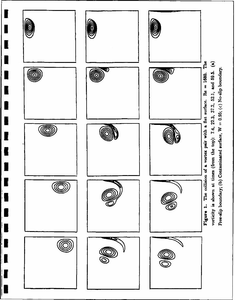
In figure 1, we show the evolution of the vorticity for three different boundary

conditions on the top surface: (a) is for a stress-free boundary; (b) for a contami-

nated surface with W = 0.95, and in (c) no-slip boundary conditions are enforced.

The vortex is initially half way between the top and bottom boundary, and the

vorticity distribution is Gaussian. In all cases, the Reynolds number is 1680. The

first frame is shortly after the motion has started, t = 7.4. For the no-slip top, a

boundary layer has already formed and vorticity is diffusing into the fluid domain.

A smaller boundary layer is also visible for the contaminated surface in (b). In the

second frame, t = 22.3, the upward motion of the vortex has ended, and, due to

the surface, it is moving outward. The boundary layers in (b) and (c) have grown

9

I

II considerably, and it is dear, in both cases, that separation is about to take place.

In the third frame, t = 37.2, the vortex in (a) continues its outward motion alongI the full-slip boundaries, but in (b) and (c) the boundary layer has separated and

formed a secondary vortex that deflects the path of the primary vortex away from

the surface. The strength of the secondary vortex, as well as the rebounding of

the primary vortex, is slightly larger for the no-slip surface in (c) than for the con-

taminated one in (b). This evolution continues in the fourth frame, t = 52.1. The

vortex in (a) moves out along the top wall, but in (b) and (c), the primary vortex

has moved further away from the top under the influence of the secondary vortex.

At the same time, the stronger primary vortex swings the secondary vortex around3so it is now almost below the primary one and thus induces an inward motion.

Viscosity has had a visible effect. The maximum vorticity of both the single vortex

in (a), as well as both vortices in (b) and (d), has decreased compared with the

previous frames. In the last frame, t = 59.5, the vortex in (a) has encountered the3 outer boundaries of the computational box and is starting to move downward along

the outer wall. In (b) and (c), the primary vortex is moving upward again, as well

* as inward.

Perhaps the most striking feature of the above sequence is the similarity between

I the corticity evolution for the contaminated surface case and the rigid-wall run. In

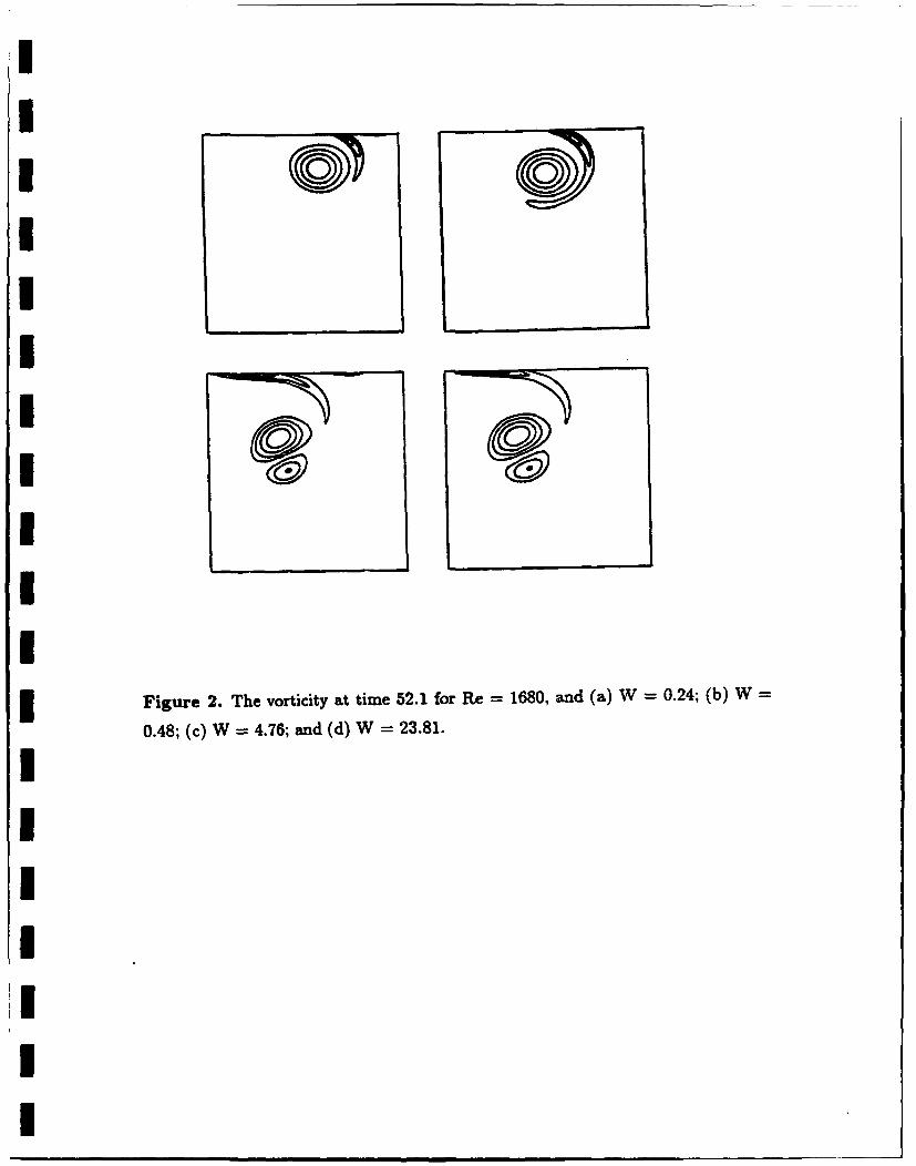
figure 2, the vorticity distribution at tine 52.1 is shown for W both larger and1 I smaller than in figure 1, and same Re. In (a), W = 0.24; (b) W = 0.48; (c)

W = 4.76; and (d) W = 23.81. In the bottom frames, where W is larger than inIfigure 1, the vorticity distribution is virtually indistinguishable from the rigid-wall

case. For smaller W in the top frames, vorticity is pulled out from the boundary but3 not enough to form a secondary vortex. The vorticity "tongue" nevertheless causes

the primary vortex to rebound slightly and therefore have lower outward velocity.I This effect increases with W.

The generation of surface vorticity is directly related to the uneven distribution

of surface contaminant. This distribution is shown in figure 3 at times correspond-

ing to those in figure 1 for all the runs in figures 1 and 2. In (a), the contaminant is

passive (corresponding to figure la) and simply advected with the flow, not causing

any shear stresses on the fluid at the boundaries. As the vortex collides with the

10

I

I surface, the contaminant is swept outward, depleting the region between and above

the vortices of contaminant and accumulating it outboard of the vortices where the

I outward velocity decreases. This contaminant peak is then pushed outward. Since

the computational box is of a finite width, the outward motion of the contaminant

is eventually slowed down by the down-welling at the outer wall of the box. Al-

though the finite box size obviously has effects on the last profiles, the maximum

contamination peak increases rapidly even before the side effects become significant.

In the second frame, (b) W = 0.24, similar evolution is seen, but the rate at which

the contaminant is pushed outward is reduced, and the maximum concentration is

much smaller. This development continues in (c) where the outward motion has

been brought nearly to a halt at the last time due to shear stress created by the

uneven contaminant distribution on the top surface. The outward motion due to

the vortices is eventually balanced by inward motion due to the uneven contaminant

distribution, slowing down the spreading of the clean region above the vortices. The

shear stress due to the contaminants creates vorticity that eventually separates and

causes the primary vortex to rebound. As the vortices rebound, their effect on the

surface diminishes, and the contamination "shock" that separates the clean and

contaminated surface starts to move inward again. In (d), the inward motion has

just started at the end of the run. The large accumulation of contaminants, seen in

frames (a) and (b), does not take place in (d), and the contamination profile behind

the shock equilibrates with time. In frame (e), W = 4.76, and the restoring effect

of the contaminants is much stronger. As a result, only a small clean region forms.

The vortices now move behind the shock, and as they pass under and rebound,

the "hole" closes rapidly. In (f), W - 23.81. Here the vortices cause only a small

depression in the contamination profile that disappears after the vortices pass by.

To investigate the difference between the results presented above in more detail,

we have collected various quantitative measures for both the vorticity and the con-

taminant distribution. In figure 4a, we plot the path of both the primary and the

secondary vortices for the no-stress case, the rigid boundary, and a number of con-

taminated surfaces. For the full-slip wall, the primary vortex moves outward until

it feels the presence of the outer boundary. For the no-slip boundaries, the path of

the primary vortex bends away from the surface as soon as a secondary vortex is

11

I

formed. When the surface is contaminated and W is large, the same rebounding

takes place, and for W = 4.76 and 23.81, the vortex paths are virtually identical

to the solid-wall case. For W = 0.95, the secondary vortex forms further outward,

and the rebounding is delayed somewhat. A distinct vortex does not form for the

lower W cases (0.24 and 0.48), but the vortex slows down and rebounds slightly,

nevertheless, due to the surface vorticity.

The total vorticity (circulation) of the same sign as the primary vortex is plotted

in figure 4b versus time. When the surface is stress free, the only way to destroy

vorticity is diffusion to the boundaries, which must remain at zero vorticity. For

no-slip and contaminated surface, the top surface not only acquires vorticity of the

I opposite sign, but this vorticity can also be convected into the fluid domain, thus

enhancing mutual destruction of vorticity. This leads to considerable increase in

I the rate of loss of primary circulation after the vortices have collided with the top

surface. Initially, the calculations with low values of W actually show higher values

I of circulation than both the no-slip and the stress-free cases. This is due to the

generation of vorticity, of the same sign as the primary vortex, at the surface where

I the contamination profile has a negative gradient. As the surface layer becomet

more immobile, this effect disappears.

* Figure 4c is a similar plot, but for the secondary vorticity. As expected, the

generation of secondary vorticity is zero for the stress-free boundary and increases

with W. Since the vortices are initiated relatively close to the surface, there is

immediately an outward velocity at the surface. For a no-slip surface, vorticity

is therefore created instantaneously, but for the contaminated surface, the surface

velocity must first redistribute the contaminant, which then, in turn, creates surface

vorticity. For the solid-wall case and the higher W's, the primary vortex eventually

rebounds, and as the vortex pair moves away from the boundary, the generation

of secondary vorticity is greatly reduced. Due to diffusion, secondary vorticity also

undergoes mutual destruction with the primary vorticity. A somewhat surprising

SI feature of the graph in figure 4c is that the curves do not approach the solid-wall case

monotonicly. In particular, the W = 4.76 case actually has more secondary vorticity

I at late times than do the W = 23.81 and the solid-wall cases. The explanation for

this is that when there is significant variations in the contamination profile, as is theJ 12

I case for W = 4.76, vorticity generation does not cease as the vortices move away

from the boundary, as in the no-slip case. The surface vorticity is still proportional

I to the contamination gradient, and remains non-zero until the contamination profile

is flat again. To separate the surface vorticity from the vorticity of the secondary

I vortex, we have estimated its strength by excluding a layer near the surface when we

integrate the secondary vorticity. For W = 4.76 and 23.81, as well as the solid-wall

I case, this gives the strength of the secondary vortex about a fourth of the strength

of the primary one. For W = 0.95, the strength is one-fifth of the primary vortex.

I The above comparisons have focused on the vorticity distribution. To quantify

the evolution of the contamination profile in a simple way, we plot in figure 5a

the second moment of the profile. If the profile remains flat, as for high W's, this

quantity remains zero; if the "hole" continues to grow, as for the stress-free surface,

it increases constantly. For W high enough so that the outward motion of the

contaminant stops, the curve levels off, eventually bending down again when the

profile starts to become flat again. As the graph shows, the profile for W = 0.24

is still changing at the end of the run, although at a considerably lower rate than

for the stress-free boundary. In all other cases, the growth has stopped and is

actually slightly negative at the end of the run. In figure 5b, we plot the position

of the contamination jump where it has formed. Since the jump is not completely

sharp (a slight artificial viscosity is used to prevent oscillations), we determine the

position simply as the point where the profile crosses a horizontal line at half the

initial concentration. The result shows what has been pointed out before, that the

outward motion stops for sufficiently high W, and the "hole" closes again at the

end of the large W runs.

The above calculations have all been done in a relatively small computational

domain. To assess the influence of the boundaries on the evolution, we have re-

peated a few of the runs in a domain that is twice as wide. In figure 6, we show

the vorticity, as well as the contamination profiles, for W = 0.95 at time 52.1 for

both the short and the long computational domain. In addition, the contamination

profiles at several times are shown at the top of the figure. The vorticity distribu-

tion is obviously almost identical, and only for the last times is there any significant

deviations in the contamination profiles. The value of the contamination concen-13

I

I tration is slightly higher behind the shock for the shorter box, and, as a result, the

shock moves slightly faster to dose the hole in the contamination profile after the

vortices have rebounded. Other cases show similar agreement. Even for a stress-free

boundary there is good agreement at early times, although at late time there are

differences, since no rebounding takes place and the vortex continues to move out-

ward in the longer box. These tests suggest that boundary effects are minimal for

the results we show, particularly for those cases where rebounding takes place. We

have also checked the effect of the initial depth of the vortex, and except that the

Iinitial deformation of the contamination profile is slower, no significant differences

arise. In particular, the maximum opening of the contaminant "hole" and the path

Iof the vortices remain essentially unchanged. (For low Reynolds numbers, diffusion

has had longer time to modify the vorticity distribution; at higher Re, this effect is

I insignificant).

All the calculations presented so far have been at a Reynolds number of 1680.

This number reflects a compromise between our desire to consider as high Re as pos-

5 sible (since experiments are usually carried out at considerably higher Re), and theincreased resolution requirement, and thus computer time, for high Re calculations.

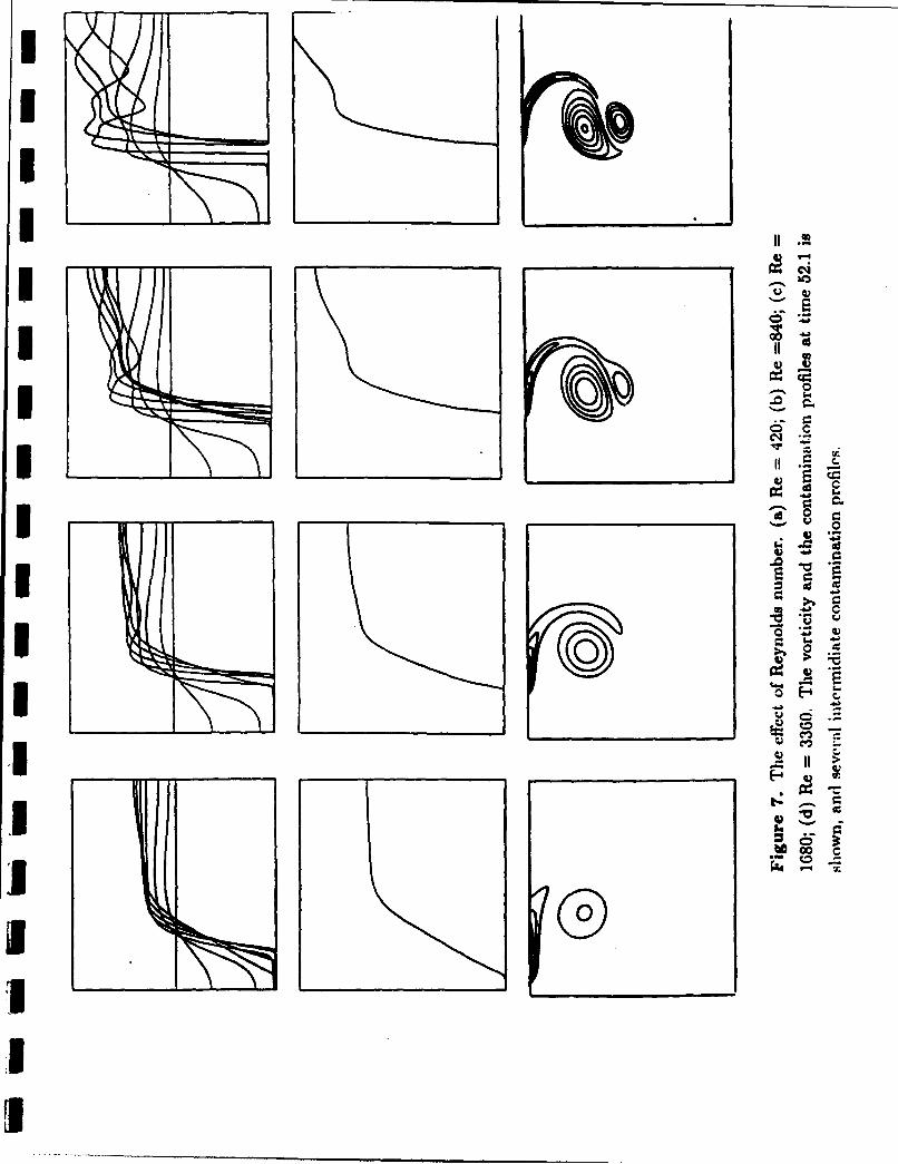
I To explore the influence of the Reynolds number, we have compared calculations

with W = 0.95 and Re = 420, 840 and 3360, with the results from figure lb and 3d

I (Re = 1680). The vorticity distribution at time 52.1 and the contamination profiles

for selected times are shown in figure 7. Again, the contaminant profile at the last

I time is shown separately for easier comparison. Obviously, the vortices diffuse faster

the smaller the Reynolds number. In 7a (Re = 420), the primary vortex has almost

fully disappeared, and no secondary vortex is visible. In 7b (Re = 840), there is

only a small "tongue" of secondary vorticity, whereas in 7c (Re = 1680) a distinct

secondary vortex has formed. For the highest Reynolds number in 7d (Re = 3360),

this secondary vortex is even stronger. The change in vorticity is reflected in the

contamination profiles. In all cases, a clean region is generated above the vortex

center, but the maximum width of this region increases with Reynolds number, and

the reclosing is delayed.

In 8a, the trace of the position of the maximum vorticity is shown. For low Re, no14

I

I secondary vortices form, and the primary vortex slows down rapidly as its circulation

diminishes. Since vorticity diffuses rapidly toward the top surface, the position of

maximum vorticity does not reach as close to the surface as the stronger vortices at

higher Reynolds number do, and actually an apparent rebounding, due to this effect,

I takes place at the end of the run. The high Re vortices first move outward parallel to

the free surface but then take a rather sharp downward turn as the secondary vortex

I appears. The effect of vorticity diffusion is clear in figure 8b where the integral of

all vorticity of the same sign as the primary vorticity is plotted versu. time. For all

I cases, the rate of diffusion changes significantly once secondary vorticity of opposite

sign has been generated. For the highest Reynolds number, there is actually a slight

I increase in the total vorticity initially; this is due to negative vorticity generated

at the surface, where the contaminant profile exhibits a negative gradient. Such

negative vorticity is also generated for lower Re but does not contribute enough to

increase the total negative vorticity. The growth of the secondary vorticity, figure

8c, is initially largest for low Re where the surface vorticity diffuses most rapidly

into the domain. However, as the strength of the primary vortex is reduced, the

rate at which secondary vorticity is produced decreases. Although little secondary

vorticity is created initially for the high Reynolds numbers, the production increases

* rapidly as separation takes place. As the primary and secondary vortex rebound,

the rate at which secondary vorticity is produced decreases again. The Reynolds

number effects on the contamination profile is quantified in figure 9, where the

second moment is plotted versus time. In all cases, there is a considerable growth

in this quantity, reflecting that the distribution forms a clean hole. The variations

are smallest for the low Reynolds numbers and start first to decline for those cases,

since the contamination begins to equilibrate first there. For low Reynolds numbers,

diffusion is more effective than rebounding in reducing the influence of the vortices

on the surface contaminant. Up to about time 20, there is relatively small difference

in the contamination for the largest Re.

I Notice that the comparison presented in figures 7-9 is not directly representative

of an experimental condition where the Reynolds number is increased by eitherincreasing the strength of the vortices or decreasing the viscosity of the liquid.

Since both r and p enter into W, it would generally change also, whereas here we15

keep W constant. A comparison for such a situation, where W changes as a result

of change in viscosity, is given by comparing figure 7d, and figure 2b (and 3c). In

the calculations in 2b relatively little secondary vorticity forms, and the "hole" in

the contamination profile continues to grow. Obviously there is much less similarity

between these cases than the cases shown in figure 7c and 7d. Changing r, while

keeping everything else corresponds to comparing the Re = 3360, W = 0.95 run

to W = 1.90 at Re = 1680, which would make the hole even smaller, and the

agreement worse.

Although there are still considerable differences between the results for the high-

est Reynolds numbers in the calculations in figure 7, the similarities are actually

more striking than the differences. Furthermore, the changes between Re = 1680

and Re = 3360 are noticeably smaller than between 840 and 1680. In addition to

that, the major differences are near the end of the runs. We are therefore tempted

to make the conjecture that as the Reynolds number increases with W constant, the

solution becomes independent of Re for a time that becomes longer as the Reynolds

number becomes larger. This is similar to what is observed for a number of other

flows and simply suggests that vorticity diffusion has not had time to modify the

flow in a significant way. Finite viscosity is, of course, essential to balance the

stresses at the surface created by the variation in surface tension. However, both

the surface-tension-generated shear and the viscosity enter into W, and if viscosity

is reduced, a "stronger" contaminant must be used to keep W constant. The same

argument applies to the circulation, r, which also appears in W. This conjecture

will be the basis for our comparisons with the experiments of Willmarth and Hirsa

(1990).

At late times, there will always be considerable dependency on the Reynolds

number. In particular, the vortices are more long-lived the higher the Reynolds

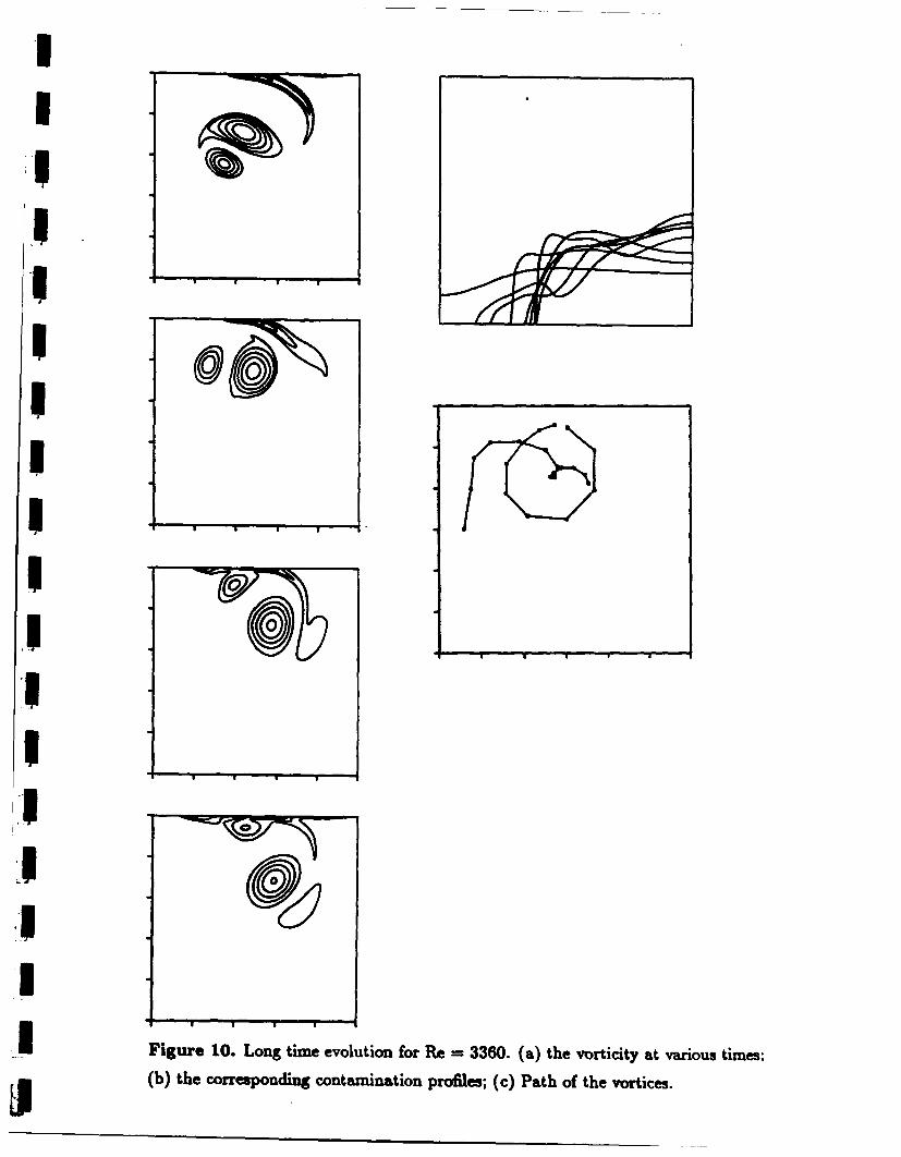
number. We have continued the Re = 3360 calculations up to much longer time

than the lower Re calculations and show selected frames, at late times, in figure 10a,

as well as the corresponding contamination distribution in 10b. The initial evolution

is much like the run shown in figure lb; the primary vortex generates a secondary

vortex that causes rebounding. Since the secondary one is much weaker than the

primary one, the path curves inward as the secondary vortex is swung around the16

I

I primary one eventually bringing both vortices back to the surface. The secondary

vortex has now diffused considerably, but the primary one is still strong and causes

i a tertiary vortex to form. This tertiary vortex, although relatively weak, again leads

to rebounding. The path of the vortices is plotted in figure 10c and shows that the

primary vortex actually rebounds further away from the centerline than the second

time. As the vortex pair comes back the second time, the contamination shock is in5 the process of moving back inward. While the front of the shock continues to move

inward partly assisted by the secondary vortex, the primary vortex pushes the rest

5of the contaminant outward, thus creating the "hump' in the profile.

3 Long time calculation of the collision of a vortex pair with a rigid, no-slip wall

have been reported by Orlandi (1990). The vortices in his calculations loop back3 closer to the centerline than in figure 10 leading to an ejection of the secondary

vortices for sufficiently high Reynolds numbers. The result in figures 1, 2 and 4a

suggest that similar behavior would be observed here for higher W's (and the no-slip

run) if the calculations were continued to later time.

.1 3.2 Comparison with experiments

A detailed experimental study of the situation discussed in the previous section

has been undertaken by Willmarth and Hirsa (1990). They experimented with a

vortex pair generated by a pair of flaps mounted in a water tank and made a number

of detailed measurements of both the vortex motion and the free surface signature.

- In addition to visualization by LF, the velocity field was measured using particle

image velocimetry. Extensive investigations of the three-dimensional evolution of

I a vortex pair colliding with a free surface were also done, but our two-dimensional

calculations are only pertinent to the two-dimensional aspects.

I The calculations of the preceding section were for rather low Reynolds number

and used a simple constitutive equation for the contaminants. Willmarth and Hirsa

used exactly determined quantities of oleyl alcohol to vary the surface contaminant

in a predetermined way and made detailed measurements of the surface tension for

a given amount of surfactant. We have fitted an analytic expression to the measure-

ments of Hirs (1990), and figure 11 shows the curve along with the experimentally* 17

I

determined points. The curve consists of three parts,

70.838, if c < 0.828 x 10-7;a(c) 45.08 + 62.22c - 37.575c 2, if 0.028 x 10 < c < 1.242 x 10-7; (7)

103.03 - 31.11c, if c > 1.242 X 10-7;

Hirsa's measurements agrees well with data in Gaines (1966). The Reynolds number

of.the experiments ranged from 12,000 to 17,000, which would require excessive res-

olution, in particular since our calculations were all done on a regular grid. However,

as observed in figure 7 and 8 the evolution appears to be relatively insensitive to

the Reynolds number once it is sufficiently high. We have therefore run a case com-

parable with the experimental setup but kept the Reynolds number as well as the

computational domain considerably smaller than in the experiments (Re = 7000,

and a 256 by 256 grid). W was, on the other hand, kept the same as in the exper-

iments. The initial contamination concentration is c. - 0.848 x 10- 7. The initial

conditions for the vorticity came from the experimentally determined velocity field.

The results are shown in figure 12, where the vortex path, as well as the extend of

the clean region above the vortices, is compared with the experimental results.

There are some differences. The maximum "opening" of the contaminant layer

is smaller in the computations than in the experiments, and as a consequence, the

secondary vortex forms closer to the centerline, and the primary vortex rebounds

more. In addition to equation (7), we have also used slightly different analytical

fits for the contaminant equation of state and find considerable sensitivity. It is

therefore likely that a minor change in the equation of state would lead to a better

agreement. A careful examination of figure 11 suggest that a slightly smaller slope,

around c = 0.1 x 106, would be consistent with the experimental data. Such change

would lead to changes in the right direction. We have elected to present these re-

sults, nevertheless, because we feel that they represent the level of agreement that

i may be expected without any "tuning" of the fit. Furthermore, this calculation is

where the solution shows most sensitivity to small changes in W. Therefore, al-

though the agreement is not perfect, we feel that it is as good as can be expected in

this parameter range without unreasonable "tuning" of the a(c) fit. We also note

that the experimental results come from one realization, but the vorticity used to

initialize the computations from another one. Although the experiments were rela-

tively repeatable, the results showed some scatter presumably due to longitudinal18

I

I undulations of the vortices (see Willmarth and Hirsa, 1990).

3.3 Axisymmetric vortex rings

The main focus in this paper is on two-dimensional vortex pairs. As discussed by

Bernal, Hirsa, Kwon, and Willmarth (1989), axisymmetric vortex rings are similarly

affected by contaminants on the free surface. The major difference from the planar3 case is the stretching of the vortex ring as it moves outward along the top boundary.

This stretching opposes the increase in the core size by diffusion and does lead to3vorticity intensification for high enough Reynolds numbers.

We have done a few calculations for axisymmetric rings, and figure 13 shows two

examples. In (a) the top surface is stress-free and in (b) W = 3.6. The Reynolds

number is 2000 in both cases, and the computational box is relatively small The3 evolution is similar to the two-dimensional case; in the simulation with stress-free

boundaries the vortex moves outward to the outer boundaries but rebounds when3the surface is contaminated. Since the vortex ring expands as it moves outward,

diffusion of vorticity is countered by vorticity intensification by stretching. For the

3stress-free surface our calculations are in good agreement with those of Orlandi

(1990).

1 3.4 Oblique collisions of vortex pairs

All the computations discussed so far involve a vortex pair colliding head on.U1with the surface. To show that the basic interaction mechanisms are insensitive

to the exact angle of approach, we have run one case where the vortices approach

the surface at an 450 angle. The results are shown in figure 14. Here Re = 1680

and W = 0.95. Initially the top vortex has more influence on the contaminant

distribution, and the contaminant is mostly pushed to the right. When this vortex

is sufficiently close to the surface it starts to move backwards (to the right) due

to the effect of its image and in the process scoops up vorticity from the boundary

layer created by the uneven contaminant distribution. It then rebounds. The second

vortex has now come closer to the surface--so the vortex pair is actually facing the

surface more directly-and pulls vorticity from the boundary layer. This vortex

does not make it as close to the surface as the first one, since its partner has left

it, and the secondary vortex is much weaker than for the partner. Consequently,19

I

I the rebound of the second vortex is much smaller than for the first one. While

the second vortex continues to move slowly to the left, the first vortex has swept

its secondary vortex around itself, as well as moved in a small loop. It therefore

collides with the surface again pulling out a tertiary vortex. The secondary vortex

has in the mean while diffused away and reduced the circulation of the primary

one. We are now left with essentially one vortex that moves slowly down and to

I the left. The contamination shock on the right moves back in to close the hole, but

on the left, the shock has become essentially stationary in the last frame. A careful

examination of the location of the right shock shows that the looping of the primary

vortex is reflected in slight oscillation of the location of the shockL

This example suggest that the behavior observed in the head on collisions studied

earlier in the paper is actually stable to variations in the approach angle. Although

there are some difference for the rather extreme case of 45° , these are of a relatively

obvious nature.

4. Conclusions

I We have investigated in some detail the influence of a free surface contamina-

tion on the motion of a vortex pair toward a wave-less free surface. Several two-

I dimensional simulations for various values of the governing nondimensional num-

bers, Re and W, have been done. The main observations of the present work are aU confirmation of the experimental results of Bernal et al (1989) and Willmarth and

Hirsa (1990) that contamination of the free surface can alter the submerged vorticalU motion in a fundamental way. Our use of a very simple equation of state for the

contaminant suggest that this is a generic property of contaminated free surface

I flows.

Although our calculations have been limited to a somewhat low Reynolds num-ber, the results suggest that at early times and high enough Reynolds numbers the

evolution depends primarily on W and only weakly on Re. For low W, the sur-

face contaminant is redistributed considerably by the flow, but for higher W the

surface resists the motion, acting more or less like a rigid wall in the limit of very

high W. Intermediate values results in localized clean regions, separated from the

contaminated surface by a sharp "shock." Of course, for long enough time, Re will20

I

I eventually determine the rate of decay of the vorticity." For all Re that we have

simulated, the addition of contaminant greatly increases the rate of decay of the

I circulation of the primary vortex. Generally, shortly after generation the secondary

vortices have strength about a fourth to a fifth of the primary vortex, which is

Im consistent with the single measurement taken by Hirsa (1990). For large enough

W, the contaminant distribution remains almost flat for all time, and the evolution

3 of the vortical flow is nearly indistinguishable from the no-slip case. Therefore, at

high Re and W we expect the evolution to be independent of the actual value of

I these parameters.

The major limitation of this study is that the free surface has been taken as flat.

This limits the applicability of the predictions to small Froude numbers. However,

the comparison with the experiments of Willmarth and Hirsa (1990) suggests that

I this approximation does not bias the results in any significant way.

Although the main conclusion from this study is a conformation of the mecha-

nism already explained experimentally by Bernal et al (1989) and Willmarth and

Hirsa (1990), we note that the flexibility of the numerical approach has allowed us

to obtain information that is extremely difficult, expensive, and time consuming to

measure (e.g. how the distribution of the surface contaminant changes with time),

and to explore parameter combinations difficult to realize experimentally (e.g. the

shape and magnitude of a(c)).IAcknowledgment

j This work was supported by the Program in Ship Hydrodynamics (PSH) at The

University of Michigan, funded by the University Research Initiative of the Office of

31 Naval Research (contract No. N000184-86-K-0684). Constructive interaction with

Professors L. Bernal and W.J.A. Dahm and other member of the PSH has been

I most helpful in carrying out the research discussed here. G.T. would like to thank

P. Orlandi for discussions and for sending preprints of his work. The calculations

3l were done mostly on the computers at the San Diego Supercomputer Center, which

is sponsored by the NSF.I.2

j 21

I

i References

Barker, S. J. and Crow, S. C. 1977. The motion of two-dimensional vortex pairs

in a ground effect. J. Fluid Mech. 82, 659-671.

Bernal, L. P., Hirsa, A., Kwon, J. T. and Willmarth, W. W. 1989. On theinteraction of vortex rings and pairs with a free surface for various amounts of

a surface active agent. Phys. Fluids A 4, to appear.

Bernal, L. P. and Madnia, K. 1989. Interaction of a turbulent round jet with the3 free surface. In Proceedings of 17th Syrnp. on Naval Hydrodynamics, National

Academy Press, Washington, D.C., 79-87.

Bernal, L. P. and Kwon, J. T. 1989. Vortex ring dynamics at a free surface.

Phys. Fluids A 1,449-451.

3 Dahm, W. J. A., Scheil, C. M. and Tryggvason, G. 1989. Dynamics of vortex

interaction with a density interface. J. Fluid Meck. 205, 1-43.

I Davies, J. T. 1966. The effects of surface films in damping eddies at a free

surface of a turbulent liquid. Proc. of the Roy. Phys. Soc. A 290, 515-526.

I Davies, J. T. and Driscoll, J. P. 1974. Eddies at free surfaces, simulated by

pulses of water. Ind. Eng. Chem., Fundam., 13, 105-109.

Gaines, G.L. Jr., 1966. Insoluble monolayers at liquid-gas interface. Inter-

I science.

J.F. Harper, The motion of bubbles and drops through liquids. Adv. AppL

3 Mech. 12 (1972), 59-129.

Harvey, J.K. and Perry, F.J. 1971 Flowfield produced by trailing vortices in the

I vicinity of the ground. AIAA J. 9, 1659-1660.

Hirsa, A. 1990. An experimental investigation of vortex pair interaction with a

dean and contaminated free surface. Ph.D. Thesis. The University of Michigan.

Hirsa, A., fryggvason, G., Abdollahi-Ahlbeik, J., and Willmarth, W.W. 1990.

I Measurement and computations of vortex pair interaction with a clean or con-

taminated free surface. In Proceedings of 18th Symp. an Naval Hydrodynamics,

I National Academy Press, Washington, D.C., xx-xx.

Marcus, D. L. and Berger, S.A. 1989. The interaction between a pair of counter-22

I

I rotating vortex pair in vertical ascent and a free surface. Phys. Fluids A 1,

1988-2000.

Ohring, S. and Lught, H.J., 1989. Two counter-rotating vortices approaching

a free surface in a viscous fluid. David Taylor Research Center Rep. DTRC-

89/019, Bethesda, MD.

Orlandi, P. 1990. Vortex dipole rebound from a wall. Phys. Fluids A x, xx-xx.

Orlandi, P. 1990. Vortices interacting with non-slip walls: Stirring and mixing

of a passive scalar. (preprint).

Orlandi, P. 1990. Vortex rings impinging walls. (preprint).

I Ostrach, S. 1982. Low-gravity fluid flows. Ann. Rev. Fluid Meek. 14, 313-345.

Peace, A. J. and Riley, N. 1983. A viscous vortex pair in ground effect. J. Fluid

Mech. 129, 409-426.

Scott, J.C. 1982. Flow beneath a stagnant film on water: the Reynolds ridge.

J. Fluid Meek. 116, 283-296.

Safman, P. G. 1979. The approach of a vortex pair to a plane surface in inviscid

fluid. J. Fluid Meek. 92, 497-503.

U Sarpkaya, T. 1986. Trailing-vortex wakes on the free surface. 16th Symposium

on Naval Hydrodynamics, National Academy Press, 38-50.

I Sarpkaya, T., Elnitsky II, J. and Leeker Jr., R. E. 1989. Wake of a vortex pair

on the free surface. Seventeenth Symposium on Naval Hydrodynamics, National

Academy Press, Washington, D.C., 53-60.

I M. Song, L. Bernal, and G. "Iryggvason. 1990. Head-ca collision of a large

vortex ring with a free surface. URI Report 90-x.

I H.A. Stone and L.G. Leal. The effects of surfactants on drop deformation and

breakup. (preprint, 1989).

1 Telste, J. H. 1989. Potential flow about two counter-rotating vortices approach-

ing a free surface. J. Fluid Meek. 201, 259-278.

I Tryggvason, G. 1988. Deformation of a free surface as a result of vortical flows.

Phye. Fuids 31, 955-957.

I

I

I Wang, H.T. and Leighton, R.I 1990. Direct calculation of the interaction be-

tween subsurface vortices and surface contaminants. Proceedings of the 9th.

OMAE Conference, Houston TX, Feb 1990, Vol. I, Part A.

Willmarth, W. W., Tryggvason, G., Hirsa, A. and Yu, D. 1989. Vortex pair

generation and interaction with a free surface. Phys. Fluids A 1, 170-172.

Willmarth, W. W., and Hirsa, A. 1990. (In preparation).

Yu, D. and Tryggvason, G. 1990. The Free Surface Signature of Unsteady,

Two-Dimensional Vortex flows. J. Fluid Mech., 218, 547-572.

2IIIIIIIIII

I 2

I

I Figure Captions

Figure 1. The collision of a vortex pair with a flat surface. Re = 1680. Thevorticity is shown at times (from the top): 7.4, 22.3, 37.2, 52.1, and 59.5. (a)5 Free-slip boundary. (b) Contaminated surface, W = 0.95. (c) No-slip boundary.

Figure 2. The vorticity at time 52.1 for Re = 1680, and (a) W = 0.24; (b) W -5 0.48; (c) W = 4.76; and (d) W = 23.81.

Figure 3. The contaminant profile at times 7.4, 22.3, 37.2, 52.1, and 59.5, for theruns in figure 1 -nd 2. (a) Free-slip surface; (b) W = 0.24; (c) W = 0.48; (d) W -

0.95; (e) W = 4.76; (f) W = 23.81;

IFigure 4. (a) The path of the vortices for the runs in the previous figures. (b)Vorticity of the same sign as the primary vortex, integrated over the computationaldomain versus time. (c) Integrated secondary vorticity versus time. full slip;- - - W = 0.24; ---- W = 48; -...- - W=0.95; - - --W=4.76; - - - Wp23.81; - no slip.

Figure 5. (a) The second moment of the contamination profile, f(c - Co) 2dx versustime for the runs in the previous figures. (b) The contaminant jump versus timefor the cases where a clean "hole" forms.

I Figure 6. The solution for Re=1680 and W=0.95 at time 52.1 as calculated bothin a short and a long computational domain. The contamination profiles are alsoshown for several intermidiate times.

Figure 7. The effect of Reynolds number. (a) Re = 420; (b) Re =840; (c) Re -

1680; (d) Re = 3360. The vorticity and the contamination profiles at time 52.1 isshown as well as several intermediate contamination profiles.

Figure 8. The effect of Reynolds number. (a) The path of the vortices for theruns in the previous figure. (b) Vorticity of the same sign as the primary vortex,integrated over the computational domain versus time. (c) Integrated secondaryvorticity versus time.

I Figure 9. The second moment of the contamination profile, f(c - c.) 2dz versustime, for the runs in figure 7.

Figure 10. Long time evolution for Re = 3360. (a) The vorticity at various times.p(b) The corresponding contamination profiles; (c) Path of the vortices.

25

I

I

I Figure 11. Comparison with experiments, analytical fit to the a(c) curve andthe measuirements of Hirsa (1990) (squares and circles). The initial contaminantconcentration is 0.843 x 10-6 cm 3 /cm 2 .

Figure 12. Comparison with experiments, Vortex paths, and the extend of theclean "hole" in the contaminant layer.

Figure 13. The evolution of an axisymmetric vortex ring with (a) clean surfaceand (b) contaminated surface

Figure 14. Oblique collision of a vortex pair with a contaminated surface. Thevorticity is shown at selected times in (a) and the corresponding contaminationprofiles in (b).

IIIIIIII

I1 2

I.

cIC

-0 0

* _ _ _ _ __ _ _ cq

I .2

E4

_ _ _ _ _ _ _ _ _ _ _ _ _ _ _ _ _ o

_ _ _ _ ~ - W k

II ______________ ______________

*III _____________

IUII3 Figure 2. The vorticity at time 52.1 for Re = 1680, and (a) W = 0.24; (b) W =

0.48; (c) W 4.76; and (d) W = 23.81.

IIUIIIU

UIIII ______________ ______________

IIIU _______________

IIIII

Figure 3. The contaminant profile at times 7.4, 22.3, 37.2, 52.1, and 59.5, for the

runs in figure 1 and 2. (a) Free-slip surface; (b) W = 0.24; (c) W = 0.48; (d) W =3 0.95; (e) W = 4.76; (f) W = 23.81;

UII

/ 4,. 4i

/ *~ * />

44 >

>b

V 0

/4C C: .

4 C4

a a&

Ib

O.S--

~Ole

0. ~40.. .0 .1 0.0 10

Fiur 5.(a hescodmoet f h cnamntinprfie fc- .2d eru

tieIo h u ntepeiu iues b h otmnn upvru iefoIh ae hr la hl"frs

Ux

U1 . 9

I r.

* 4a0

0

Ao.

II _

II* I U ~

00 ~I IIV V

~ 0II ~

~ *~~C..*

V C

I C ~1

C 0 ~It~4

___ oE~tV c.~

-

V'I .C II >

I .~ CC

~ -C

~o0 C

1 0I1III

I _________

I '~ ,'

'. '

I ' '%~%~

I4) -AX~

4)

a..4.) 4.)I...EU0 ~~

I~1

C Mi- *: , 0.~I ~4Q2 ~3

/ 4) 4): / .. ~ s::;I:,~ ~: ~ 0

/

I~ _ .~ I.6

ii,i: / 4.) 0 ~I U,*: I

*-. 0

I

I I 0 0* S * I

1*.g I-.I4) 0 -~ .~

.- .4.)4) ~.

0 ~.0V 4)

'S.1 *~ ~ .4.)

*

.4 0I,

IIU ________

II

III

2.67-

I -.00

0o00 ....

0.000. 20. 40. 60.

Figure 9. The second moment of the contamination profile, f(c - c.) 2dz versus

time, for the runs in figure 7.

IIIII.

I

II

I 0m-

,

n Figure 10. Long time evolution for Re -- 3360. (a) the vorticity at various times:

(b) the corresponding contamination profiles; (c) Path of the vortices.

7IA

I00

450

UU

III

I

1 l expeib)e~l*1

,

I

-1.02.

o---0 expfere

Figure 12. Comparison with experiments, "Vortex paths. and the extend of theclean "hole" in the contaminant layer.

II

I 4

'I _ _ _ _ _ _ _ _ _ _ _ _|

1 .0

II U

I -ifi

.. I. 0

I! _________

Iii

* 00

.r'. i

Figure 1L4. Oblique collision of a vortex pair with a contaminated surface. The

m vrticity is shown at selected times in (a), and the corresponding contamination

profiles in (b).

III

UIU

I (bl_______________IIIIIIIIIILI