sssnet: semi-supervised signed network clustering

SSSNET: Semi-Supervised Signed Network Clustering

Yixuan He∗ Gesine Reinert† Songchao Wang‡ Mihai Cucuringu§

AbstractNode embeddings are a powerful tool in the analysis ofnetworks; yet, their full potential for the important task ofnode clustering has not been fully exploited. In particular,most state-of-the-art methods generating node embeddingsof signed networks focus on link sign prediction, and thosethat pertain to node clustering are usually not graph neuralnetwork (GNN) methods. Here, we introduce a novelprobabilistic balanced normalized cut loss for training nodesin a GNN framework for semi-supervised signed networkclustering, called SSSNET. The method is end-to-end incombining embedding generation and clustering without anintermediate step; it has node clustering as main focus, withan emphasis on polarization effects arising in networks. Themain novelty of our approach is a new take on the roleof social balance theory for signed network embeddings.The standard heuristic for justifying the criteria for theembeddings hinges on the assumption that an “enemy’senemy is a friend”. Here, instead, a neutral stance isassumed on whether or not the enemy of an enemy is afriend. Experimental results on various data sets, including asynthetic signed stochastic block model, a polarized versionof it, and real-world data at different scales, demonstratethat SSSNET can achieve comparable or better results thanstate-of-the-art spectral clustering methods, for a wide rangeof noise and sparsity levels. SSSNET complements existingmethods through the possibility of including exogenousinformation, in the form of node-level features or labels.

Keywords: clustering, signed networks, signed stochastic

block models, graph neural networks, generalized social

balance, polarization.

1 Introduction

In social network analysis, signed network clustering isan important task which standard community detectionalgorithms do not address [45]. Signs of edges in net-works may indicate positive or negative sentiments, seefor example [43]. As an illustration, review websites aswell as online news allow users to approve or denounceothers [34]. Clustering time series can be viewed as aninstance of signed network clustering [1], with the em-pirical correlation matrix being construed as a weightedsigned network. For recommendation systems, [47] in-troduced a principled approach to capturing local andglobal information from signed social networks mathe-matically, and proposed a novel recommendation frame-work. Recently interest has grown on the topic of polar-ization in social media, mainly fueled by a large variety

∗[email protected]; Univ. of Oxford (UoOx).†[email protected]; UoOx & The Alan Turing Inst. (ATI).‡[email protected]; Univ. of Sci. and Tech. of China.§[email protected]; UoOx & ATI.

of speeches and statements made in the pursuit of pub-lic good, and their impact on the integrity of democraticprocesses [54]; our work also contributes to the growingliterature of polarization in signed networks.

Most competitive state-of-the-art methods generat-ing node embeddings for signed networks focus on linksign prediction [29, 11, 55, 33, 9, 57, 17], and thosethat pertain to node clustering are not GNN methods[51, 55, 32, 12, 14]. Here, we introduce a graph neu-ral network (GNN) framework, called SSSNET, witha Signed Mixed-Path Aggregation (SIMPA) scheme, toobtain node embeddings for signed clustering.

The main novelty of our approach is a new takeon the role of social balance theory for signed networkembeddings. The standard heuristic for justifying thecriteria for the embeddings [55, 10, 17, 35, 26, 27]hinges on social balance theory [22, 44], or multiplicativedistrust propagation as in [20], which asserts that in asocial network, in a triangle either all three nodes arefriends, or two friends have a common enemy; otherwiseit would be viewed as unbalanced. More generally, allcycles are assumed to prefer to contain either zero oran even number of negative edges. This hypothesisis difficult to justify for general signed networks. Forexample, the enemies of enemies are not necessarilyfriends, see [20, 46]; an example is given by the socialnetwork of relations between 16 tribes in New Guinea[40]. Hence, the present work takes a neutral stance onwhether or not the enemy of an enemy is a friend, thusgeneralizing the atomic propagation by [20].

From a method’s viewpoint, the neutral stance isreflected in the feature aggregation in SIMPA, whichprovides the basis of the network embedding. Networkclustering is then carried out using the node embeddingas input and a loss function for training; see Figure1 for an overview. To train SSSNET, the loss func-tion consists of a self-supervised novel probabilistic bal-anced normalized cut loss acting on all training nodes,and a supervised loss which acts on seed nodes, if avail-able. Experimental results at different scales demon-strate that our method achieves state-of-the-art perfor-mance on synthetic data, for a wide range of networkdensities, while complementing other methods throughthe possibility of incorporating exogenous information.Tested on real-world data for which ground truth is

Copyright © 2022 by SIAMUnauthorized reproduction of this article is prohibited

arX

iv:2

110.

0662

3v3

[cs

.SI]

23

Feb

2022

MLP

𝑿𝒱 ∈ ℝ𝑛×𝑑𝑖𝑛

MLP

MLP

MLP

𝑯𝑠+

𝑯𝒔−

𝑯𝑡+

𝑯𝑡−

SIMPA

ഥ𝑨𝑠+

ഥ𝑨𝑠−

ഥ𝑨𝑡+

ഥ𝑨𝑡−

Linear Softmax Argmax

𝒁𝒱s+

𝒁𝒱s−

𝒁𝒱

𝒁𝒱t+

𝒁𝒱t−

CONCAT

𝑨 ∈ ℝ𝑛×𝑛

h ∈ ℤ+

Embedding

Probability Matrix

Cluster Assignment

Network embedding, triplet loss etc.

Probabilistic balanced normalized cut loss, cross entropy loss on seeds etc.

ARI, predicted labels, unhappyratio etc.

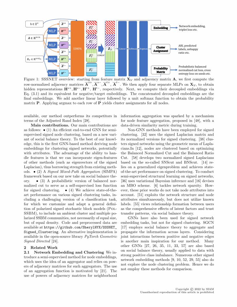
Figure 1: SSSNET overview: starting from feature matrix XV and adjacency matrix A, we first compute the

row-normalized adjacency matrices As+,A

s−,A

t+, A

t−. We then apply four separate MLPs on XV , to obtain

hidden representations Hs+,Hs−,Ht+, Ht−, respectively. Next, we compute their decoupled embeddings viaEq. (3.1) and its equivalent for negative/target embeddings. The concatenated decoupled embeddings are thefinal embeddings. We add another linear layer followed by a unit softmax function to obtain the probabilitymatrix P. Applying argmax to each row of P yields cluster assignments for all nodes.

available, our method outperforms its competitors interms of the Adjusted Rand Index [28].

Main contributions. Our main contributions areas follows: • (1) An efficient end-to-end GNN for semi-supervised signed node clustering, based on a new vari-ant of social balance theory. To the best of our knowl-edge, this is the first GNN-based method deriving nodeembeddings for clustering signed networks, potentiallywith attributes. The advantage of the ability to han-dle features is that we can incorporate eigen-featuresof other methods (such as eigenvectors of the signedLaplacian), thus borrowing strength from existing meth-ods. • (2) A Signed Mixed-Path Aggregation (SIMPA)framework based on our new take on social balance the-ory. • (3) A probabilistic version of balanced nor-malized cut to serve as a self-supervised loss functionfor signed clustering. • (4) We achieve state-of-the-art performance on various signed clustering tasks, in-cluding a challenging version of a classification task,for which we customize and adapt a general defini-tion of polarized signed stochastic block models (Pol-SSBM), to include an ambient cluster and multiple po-larized SSBM communities, not necessarily of equal size,but of equal density. Code and preprocessed data areavailable at https://github.com/SherylHYX/SSSNET_Signed_Clustering. An alternative implementation isavailable in the open-source library PyTorch GeometricSigned Directed [24].

2 Related Work2.1 Network Embedding and Clustering We in-troduce a semi-supervised method for node embeddings,which uses the idea of an aggregator and relies on pow-ers of adjacency matrices for such aggregators. The useof an aggregation function is motivated by [21]. Theuse of powers of adjacency matrices for neighborhood

information aggregation was sparked by a mechanismfor node feature aggregation, proposed in [48], with adata-driven similarity metric during training.

Non-GNN methods have been employed for signedclustering. [32] uses the signed Laplacian matrix andits normalized versions for signed clustering. [38] clus-ters signed networks using the geometric mean of Lapla-cians.In [12], nodes are clustered based on optimizingthe Balanced Normalized Cut and the Balanced RatioCut. [58] develops two normalized signed Laplaciansbased on the so-called SNScut and BNScut. [14] re-lies on a generalized eigenproblem and achieves state-of-the-art performance on signed clustering. To conductsemi-supervised structural learning on signed networks,[36] uses variational Bayesian inference and [16] devisesan MBO scheme. [6] tackles network sparsity. How-ever, these prior works do not take node attributes intoaccount. [51] exploits the network structure and nodeattributes simultaneously, but does not utilize knownlabels. [55] views relationship formation between usersas the comprehensive effects of latent factors and trusttransfer patterns, via social balance theory.

GNNs have also been used for signed networkembedding tasks, but not for signed clustering. SGCN[17] employs social balance theory to aggregate andpropagate the information across layers. Consideringjoint interactions between positive and negative edgesis another main inspiration for our method. Manyother GNNs [27, 26, 35, 11, 33, 57] are also basedon social balance theory, usually applied to data withstrong positive class imbalance. Numerous other signednetwork embedding methods [9, 10, 52, 29, 55] also donot explore the node clustering problem. Hence we donot employ these methods for comparison.


https://github.com/SherylHYX/SSSNET_Signed_Clustering

https://github.com/SherylHYX/SSSNET_Signed_Clustering

2.2 Polarization Opinion formation in a social net-work can be driven by a few small groups which have apolarized opinion, in a social network in which manyagents do not (yet) have a strongly formed opinion.These small clusters could strongly influence the publicdiscourse and even threaten the integrity of democraticprocesses. Detecting such small clusters of polarizedagents in a network of ambient nodes is hence of inter-est [54]. For a network with node set V, [54] introducesthe notion of a polarized community structure (C1, C2)within the wider network, as two disjoint sets of nodesC1, C2 ⊆ V, such that •(1) there are relatively few (resp.many) negative (resp. positive) edges within C1 andwithin C2; •(2) there are relatively few (resp. many) pos-itive (resp. negative) edges across C1 and C2; •(3) thereare relatively few edges (of either sign) from C1 and C2to the rest of the graph. By allowing a subset of nodesto be neutral with respect to the polarized structure,[49] derives a formulation in which each cluster inside apolarized community is naturally characterized by thesolution to the maximum discrete Rayleigh’s quotient(MAX-DRQ) problem. However, this model cannot in-corporate node attributes. Extending the approach in[7] and [14], here, a community structure (C1, C2) is saidto be polarized if (1) and (2) hold, while (3) is not re-quired to hold. Moreover, our model includes differentparameters for the noise and edge probability.

3 The SSSNET Method

3.1 Problem Definition Denote a signed networkwith node attributes as G = (V, E , w,XV), where V isthe set of nodes, E is the set of (directed) edges or links,and w ∈ (−∞,∞)|E| is the set of weights of the edges.Here G could have self-loops but not multiple edges.The total number of nodes is n = |V|, and XV ∈ Rn×din

is a matrix whose rows are node attributes. Theseattributes could be generated from the adjacency matrixA with entries Aij = wij , the edge weight, if there is anedge between nodes vi and vj ; otherwise Aij = 0. Wedecompose A into its positive and negative part A+ andA−, where A+

ij = max(Aij , 0) and A−ij = −min(Aij , 0).A clustering into K clusters is a partition of the nodeset into disjoint sets V = C0∪C1∪· · ·∪CK−1. Intuitively,nodes within a cluster should be similar to each other,while nodes across clusters should be dissimilar. In asemi-supervised setting, for each of the K clusters, afraction of training nodes are selected as seed nodes,for which the cluster membership labels are knownbefore training. The set of seed nodes is denoted asVseed ⊆ Vtrain ⊂ V, where Vtrain is the set of all trainingnodes. For this task, the goal is to use the embeddingfor assigning each node v ∈ V to a cluster containingknown seed nodes. When no seeds are given, we are

in a self-supervised setting, where only the number ofclusters, K, is given.

3.2 Path-Based Node Relationship Methodsbased on social balance theory assume that, given anegative relationship between v1, v2 and a negativerelationship between v2, v3, the nodes v1 and v3 shouldbe positively related. This assumption may be sensiblefor social networks, but in other networks such ascorrelation networks [1, 4], it is not obvious why itshould hold. Indeed, the column |∆u| in Table 1counts the number of triangles with an odd number ofnegative edges in eight real-world data sets and onesynthetic model. We observe that |∆u| is never zero,and that in some cases, the percentage of unbalancedtriangles (the last column) is quite large, such asin Sampson’s network of novices and the simulatedSSBM(n = 5000,K = 5, p = 0.1, ρ = 1.5) (“Syn”in Table 1, SSBM is defined in Section 4.1.1). Therelative high proportion of unbalanced triangles sparksour novel approach. SSSNET holds a neutral attitudetowards the relationship between v1 and v3. In contrastto social balance theory, our definition of “friends” and“enemies” is based on the set of paths within a givenlength between any two nodes. For a target node vj tobe an h-hop “friend” neighbor of source node vi alonga given path from vi to vj of length h, all edges on thispath need to be positive. For a target node vj to bean h-hop “enemy” neighbor of source node vi along agiven path from vi to vj of length h, exactly one edgeon this path has to be negative. Otherwise, vi and vjare neutral to each other on this path. For directednetworks, only directed paths are taken into account,and the friendship relationship is no longer symmetric.

Figure 2 illustrates five different paths of lengthfour, connecting the source and the target nodes. Wecan also obtain the relationship of a source node to atarget node within a path by reversing the arrows inFigure 2. Note that it is possible for a node to be botha “friend” and an “enemy” to a source node simultane-ously, as there might be multiple paths between them,with different resulting relationships. Our model aggre-gates these relationships by assigning different weightsto different paths connecting two nodes. For example,the source node and target node may have all five pathsshown in Figure 2 connecting them. Since the last twopaths are neutral paths and do not cast a vote on theirrelationship, we only take the top three paths into ac-count. We refer to the long-range neighbors whose in-formation would be considered by a node as the con-tributing neighbors with respect to the node of interest.

3.3 Signed Mixed-Path Aggregation (SIMPA)SIMPA aggregates neighbor information from con-tributing neighbors within h hops, by a weighted aver-


Positive link

Negative link

Friend to the source node

Enemy to the source node

Neutral to the source node

Source node

𝑠

𝑠

𝑠

𝑠

𝑠

𝑡

𝑡

𝑡

𝑡

𝑡

Figure 2: Example: five paths between the source(s) and target (t) nodes, and resulting relationships.While we assume a neutral relationship on the last twopaths, social balance theory claims them as ”friend” and”enemy”, respectively.

age of the embeddings of the up-to-h-hop contributingneighbors of a node, with the weights constructed inanalogy to a random walk on the set of nodes.

3.3.1 SIMPA Matrices First, we row-normalize

A+ and A−, to obtain matrices As+

and As−

, re-spectively. Inspired by the regularization discussed in[31], we add a weighted self-loop to each node and carry

out the normalization by setting As+

= (Ds+

)−1As+,where As+ = A+ + τ+I and the diagonal matrixDs+(i, i) =

∑j As+(i, j), for some τ+ ≥ 0; similarly,

we row-normalize As− to obtain As−

based on τ−.Next, we explore multi-hop neighbors by taking powers

or mixed powers of As+

and As−. The h-hop “friend”

neighborhood can be computed directly from (As+

)h,

the hth power of As+

. Similarly, the h-hop “enemy”neighborhood is computed directly from the mixed pow-

ers of h−1 terms of As+, and exactly one term of A

s−.

We denote the set of up-to-h-hop “friend” neighborhood

matrices asAs+,h = (As+)h1 : h1 ∈ 0, · · · , h, where

(As+

)0 = I, the identity matrix, and the set of up-to-h-hop “enemy” neighborhood matrices as

As−,h =

(As+

)h1 ·As− · (As+)h2 : h1, h2 ∈ H

with H = (h1, h2) : h1, h2 ∈ 0, . . . , h − 1, h1 + h2 ≤h − 1. With added self-loops, any h-hop neighbordefined by our matrices aggregates beliefs from nearbyneighbors. Since a node is not an enemy to itself, we setτ− = 0. We use τ+ = τ = 0.5 in our experiments.

When the signed network is directed, we addition-ally carry out `1 row normalization and calculate mixedpowers for (A+)T and (A−)T . We denote the row-normalized adjacency matrices for target positive and

negative as At+

and At−, respectively. Likewise, we

denote the set of up-to-h-hop target “friend” (resp. “en-emy”) neighborhood matrices as At+,h (resp. At−,h).

3.3.2 Feature Aggregation Based on SIMPANext, we define four feature-mapping functions forsource positive, source negative, target positive and tar-get negative embeddings, respectively. A source positiveembedding of a node is the weighted combination ofits contributing neighbors’ hidden representations, forneighbors up to h hops away. The source positive hid-den representation is denoted as Hs+

V ∈ Rn×d. Assumethat each node in V has a vector of features and sum-marize these features in the input feature matrix XV .The source positive embedding Zs+

V is given by

(3.1) Zs+V =

∑M∈As+,h

ωs+M ·M ·H

s+V ∈ Rn×d,

where for each M, ωs+M is a learnable scalar, and d is

the embedding dimension. In our experiments, we useHs+V = MLP(s+,l)(XV). The hyperparameter l controls

the number of layers in the multilayer perceptron (MLP)with ReLU activation; we fix l = 2 throughout. Eachlayer of the MLP has the same number d of hidden units.

The embeddings Zs−V , Zt+

V and Zt−V for source neg-

ative embedding, target positive embedding and tar-get negative embedding, respectively, are defined sim-ilarly. Different parameters for the MLPs for differentembeddings are possible. We concatenate the embed-dings to obtain the final node embedding as a n× (4d)matrix ZV = CONCAT

(Zs+V ,Zs−

V ,Zt+V ,Z

t−V). The em-

bedding vector zi for a node vi, is the ith row of ZV ,namely zi := (ZV)(i,:) ∈ R4d. Next we apply a linearlayer to ZV so that the resulting matrix has the samenumber of columns as the number K of clusters. Weapply the unit softmax function to map each row toa probability vector pi ∈ RK of length equal to thenumber of clusters, with entries denoting the probabil-ities of each node to belong to each cluster. The re-sulting probability matrix is denoted as P ∈ Rn×K .If the input network is undirected, it suffices to findAs+,h and As−,h, and we obtain the final embedding asZV = CONCAT

(Zs+V ,Zs−

V)∈ Rn×(2d).

3.4 Loss, Overview & Complexity AnalysisNode clustering is optimized to minimize a loss functionwhich pushes embeddings of nodes within the same clus-ter close to each other, while driving apart embeddingsof nodes from different clusters. We first introduce anovel self-supervised loss function for node clustering,then discuss supervised loss functions when labels areavailable for some seed nodes.

3.4.1 Probabilistic Balanced Normalized CutLoss For a clustering (C0, . . . CK−1), let x0, · · · ,xK−1denote the cluster indicator vectors so that xk(i) = 1 ifnode i is in cluster Ck, and 0 otherwise. Let L+ =D+ − A+ denote the unnormalized graph Laplacianfor the positive part of A, where D+ is a diagonal


matrix whose diagonal entries are row-sums of A+.Then xT

k L+xk measures the total weight of positiveedges linking cluster Ck to other clusters. Further,xTk A−xk measures the total weight of negative edges

within cluster Ck. Since D+−A = D+−A+ +A−, thenxTk (L+ + A−)xk = xT

k (D+ −A)xk measures the totalweight of the unhappy edges with respect to cluster Ck;“unhappy edges” violate their expected signs (positiveedges across clusters or negative edges within clusters).The loss function in this paper is related to the (non-differentiable) Balanced Normalized Cut (BNC) [12].In analogy, we introduce the differentiable ProbabilisticBalanced Normalized Cut (PBNC) loss

(3.2) LPBNC =

K∑k=1

(P(:,k))T (D+ −A)P(:,k)

(P(:,k))TDP(:,k)

,

where P(:,k) denotes the kth column of the probability

matrix P and Dii =∑n

j=1 |Aij |. As column k of P isa relaxed version of xk, the numerator in Eq. (3.2) is aprobabilistic count of the number of unhappy edges.

3.4.2 Supervised Loss When some seed nodes haveknown labels, a supervised loss can be added to the lossfunction. For nodes in Vseed, we use as a supervisedloss function similar to that in [48], the sum of a crossentropy loss LCE and a triplet loss. The triplet loss is(3.3)

Ltriplet =1

|T |∑

(vi,vj ,vk)∈T

ReLU(CS(zi, zj)−CS(zi, zk)+α),

where T ⊆ Vseed×Vseed×Vseed is a set of node triplets:vi is an anchor seed node, and vj is a seed node from thesame cluster as the anchor, while vk is from a differentcluster. Here, CS(zi, zj) is the cosine similarity of theembeddings of nodes vi and vj , chosen so as to avoidsensitivity to the magnitude of the embeddings. α ≥ 0 isthe contrastive margin as in [48]. LCE +γtLtriplet formsthe supervised part of the loss function for SSSNET,for a suitable parameter γt > 0.

3.4.3 Overall Objective Function and Frame-work Overview By combining LCE, Eq. (3.2), andEq. (3.3), the objective function minimizes

(3.4) L = LPBNC + γs(LCE + γtLtriplet),

where γs, γt > 0 are weights for the supervised part ofthe loss and triplet loss, respectively. The final embed-ding can then be used, for example, for node cluster-ing. A linear layer coupled with a unit softmax func-tion turns the embedding into a probability matrix. Anode is assigned to the cluster for which its membershipprobability is highest. Figure 1 gives an overview.

3.4.4 Complexity Analysis The matrix operationsin Eq. (3.1) appear to be computationally expensive

and space unfriendly. However, SSSNET resolvesthese concerns via a sparsity-aware implementation,detailed in Algorithm 1 in SI C.1, without explicitlycalculating the sets of powers, maintaining sparsitythroughout. Therefore, for input feature dimension din

and hidden dimension d, if d′ = max(din, d) n,time and space complexity of SIMPA, and implicitlySSSNET, is O(|E|d′h2 + 4nd′K) and O(4|E|+ 10nd′ +nK), respectively [19]. For large networks, SIMPA isamenable to a more scalable version following [18].

4 Experiments

This section describes the synthetic and real-world datasets used in this study, and illustrates the efficacy of ourmethod. When ground truth is available, performanceis measured by the Adjusted Rand Index (ARI) [28].When no labels are provided, we measure performanceby the ratio of number of “unhappy edges” to that ofall edges. Our self-supervised loss function is appliedto the subgraph induced by all training nodes. We donot report Normalized Mutual Information (NMI) [42]performance in Figure 5 (but reported in SI A.1 ) asit has some shortcomings [2], and results from the ARIand NMI from our synthetic experiments indeed yieldalmost the same ranking for the methods, with averageKendall tau 0.808 and standard deviation 0.233.

4.1 Data

4.1.1 Synthetic Data: Signed Stochastic BlockModels (SSBM) A Signed Stochastic Block Model(SSBM) for a network on n nodes with K blocks(clusters), is constructed similar to [14] but with a moregeneral cluster size definition.

In our experiments, we choose the number of clus-ters, the (approximate) ratio, ρ, between the largest andthe smallest cluster size, sign flip probability, η, andthe number, n, of nodes. To tackle the hardest cluster-ing task, all pairs of nodes within a cluster and thosebetween clusters have the same edge probability, withmore details in SI B.1. Our SSBM model can be repre-sented by SSBM(n,K, p, ρ, η).

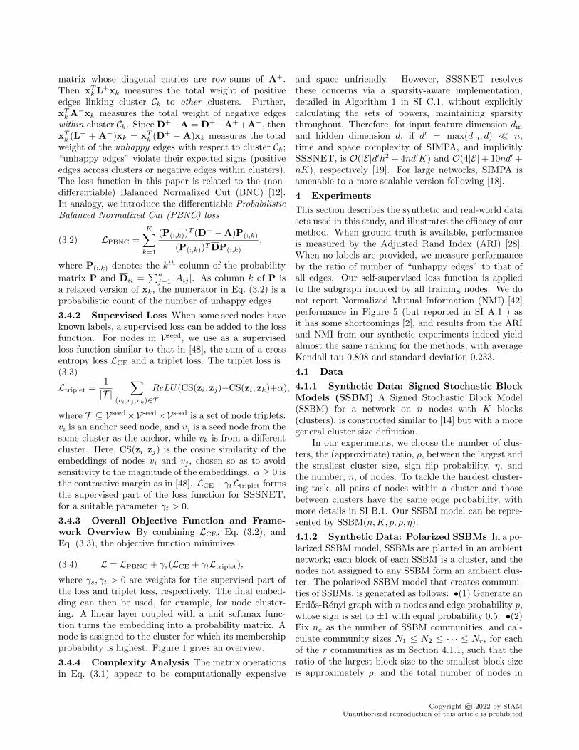
4.1.2 Synthetic Data: Polarized SSBMs In a po-larized SSBM model, SSBMs are planted in an ambientnetwork; each block of each SSBM is a cluster, and thenodes not assigned to any SSBM form an ambient clus-ter. The polarized SSBM model that creates communi-ties of SSBMs, is generated as follows: •(1) Generate anErdos-Renyi graph with n nodes and edge probability p,whose sign is set to ±1 with equal probability 0.5. •(2)Fix nc as the number of SSBM communities, and cal-culate community sizes N1 ≤ N2 ≤ · · · ≤ Nr, for eachof the r communities as in Section 4.1.1, such that theratio of the largest block size to the smallest block sizeis approximately ρ, and the total number of nodes in


these SSBMs is N ×nc. •(3) Generate r SSBM models,each with Ki = 2, i = 1, . . . , r blocks, number of nodesaccording to its community size, with the same edgeprobability p, size ratio ρ, and flip probability η. •(4)Place the SSBM models on disjoint subsets of the wholenetwork; the remaining nodes not part of any SSBM aredubbed as ambient nodes.

0 200 400 600 800 1000

200

400

600

800

1000

Sorted adjacency matrix, size 1050

1.00

0.75

0.50

0.25

0.00

0.25

0.50

1.00

3 polarized communities(SSBM K=2)

ambient nodes

0.750

(a) Sorted adjacency matrix.

0 20 40 60 80 100 120 140 160

0

20

40

60

80

100

120

140

160

Community 1 adjacency matrix, size 161

(b) Polarized community #1.

Figure 3: A polarized SSBM model with 1050 nodes,r = 3 polarized communities of sizes 161, 197, and 242;ρ = 1.5, default SSBM community size N = 200, p =0.5, η = 0.05, and each SSBM has K1 = K2 = K3 = 2blocks, rendering K = 7.

Therefore, while the total number of clusters in anSSBM equals the number of blocks, the total number ofclusters within a polarized SSBM model equals K =1 +

∑ri=1Ki = 1 + 2r. In our experiments, we also

assume the existence of an ambient cluster. Theresulting polarized SSBM model is denoted as Pol-SSBM (n, r, p, ρ, η,N). The setting in [7] can beconstrued as a special case of our model, see SI B.2.

Figure 3 gives a visualization of a polarized SSBMmodel with 1050 nodes, p = 0.5, η = 0.05, N = 200, with3 SSBMs of K = 2 blocks each, ρ = 1.5. The sortedadjacency matrix has its rows and columns sorted bycluster membership, starting with the ambient cluster.With ρ = 1.5, the largest SSBM community has size242, while the smallest has size 161, as 242

161 ≈ 1.5 = ρ.For n = 1050, the default size of a SSBM community isN = 200. For n = 5000 (resp, n = 10000) we considerN = 500 (resp. N = 2000).

4.1.3 Real-World Data We perform experimentson six real-world signed network data sets (Sampson[43], Rainfall [5], Fin-YNet, S&P 1500 [56], PPI [50],and Wiki-Rfa [53]), summarized in Table 1. Sampson,as the only data set with given node attributes (1D“Cloisterville” binary attribute), cover four social rela-tionships, which are combined into a network; Rainfallcontains Australian rainfalls pairwise correlations; Fin-YNet consists of 21 yearly financial correlation networksand its results are averaged; S&P1500 is a correlationnetwork of stocks during 2003-2005; PPI is a signedprotein-protein interaction network; Wiki-Rfa describesvoting information for electing Wikipedia managers.

We use labels given by each data set for Sampson(5 clusters), and sector memberships for S&P 1500 andFin-YNet (10 clusters). For Rainfall, with 6 clusters,we use labels from SPONGE as proxy for ground truthto carry out semi-supervised learning. For other datasets with no “ground-truth” labels available, we trainSSSNET in a self-supervised manner, using all nodesto train. By exploring performance on SPONGE, weset the number of clusters for Wiki-Rfa as three, andsimilarly ten for PPI. Additional details concerning thedata and preprocessing steps are available in SI B.

Table 1: Summary statistics for the real-world networksand one synthetic model. Here n is the number ofnodes, |E+| and |E−| denote the number of positive andnegative edges, respectively. |∆u| counts the number ofunbalanced triangles (with an odd number of negative

edges). The violation ratio |∆u||∆| (%) is the percentage

of unbalanced triangles in all triangles, i.e., 1 minus theSocial Balance Factor from [39].

Data set n |E+| |E−| |∆u| |∆u||∆| (%)

Sampson 25 129 126 192 37.16Rainfall 306 64,408 29,228 1,350,756 28.29Fin-YNet 451 14,853 5,431 408,594 26.97S&P 1500 1,193 1,069,319 353,930 199,839 28.15PPI 3,058 7,996 3,864 94 2.45Syn 5,000 510,586 198,6224 9,798,914 47.20Wiki-Rfa 7,634 136,961 38,826 79,911,143 28.23

4.2 Experimental Results In our experiments, wecompare SSSNET against nine state-of-the-art spec-tral clustering methods in signed networks mentioned inSec. 2. These methods are based on: (1) the symmetricadjacency matrix A∗ = 1

2 (A+(A)T ), (2) the simple nor-malized signed Laplacian Lsns = D−1(D+−D−A∗) and(3) the balanced normalized signed Laplacian Lbns =D−1(D+ − A∗) [58], (4) the Signed Laplacian matrixL of A∗, (5) its symmetrically normalized version Lsym

[32], and the two methods from [12] to optimize the (6)Balanced Normalized Cut and the (7) Balanced RatioCut, (8) SPONGE and (9) SPONGE sym introducedin [14], where the diagonal matrices D,D+ and D−

have entries as row-sums of (A∗)+ + (A∗)−, (A∗)+ and(A∗)−, respectively. In our experiments, the abbrevi-ated names of these methods are A, sns, dns, L, L sym,BNC, BRC, SPONGE, and SPONGE sym, respectively.The implementation details are in SI C.

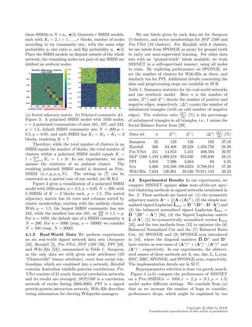
Hyperparameter selection is done via greedy search.Figure 4 (a-b) compare the performance of SSSNET

on a Pol-SSBM(n = 1050, r = 2, p = 0.1, ρ = 1.5)model under different settings. We conclude from (a)that as we increase the number of hops to consider,performance drops, which might be explained by too


0.0 0.1 0.2 0.3

0.0

0.2

0.4

0.6

0.8

ARI

234

(a) Vary hop h forSIMPA.

0.0 0.1 0.2 0.3

0.0

0.2

0.4

0.6

0.8

ARI

0.1150100500

(b) Vary γt inEq. (3.4).

0.0 0.1 0.2 0.3

0.0

0.2

0.4

0.6

0.8

ARI

00.020.050.10.51

(c) Vary seedratio.

0.0 0.1 0.2

47

48

49

unha

ppy

ratio

(%) no PBNC

w/ PBNC

(d) With/withoutthe self-supervised

part LPBNC inEq. (3.4).

0.0 0.1 0.20.0

0.2

0.4

0.6

0.8

ARI

social balance theorySSSNET

(e) Social balancetheory vs

SSSNET (as wevary η).

2 3 4 5 6K

0.2

0.4

0.6

0.8

1.0

ARI

social balance theorySSSNET

(f) Social balancetheory vs

SSSNET (as wevary K).

Figure 4: Hyperparameter analysis (a,b) and ablationstudy (c-f). Figures (a-e) pertain to Pol-SSBM(n =1050, r = 2, p = 0.1, ρ = 1.5), while Figure (f) is for anSSBM(n = 1000, η = 0, p = 0.01, ρ = 1.5) model withchanging K. Figure (d) compares the “unhappy ratio”while the others compare the test ARI.

much noise introduced. From (b), we find that the bestγt in our candidates is 0.1. See also SI C.4. Our defaultsetting is h = 2, d = 32, τ = 0.5, γs = 50, γt = 0.1, α =0.

Unless specified otherwise, we use 10% of all nodesfrom each cluster as test nodes, 10% as validationnodes to select the model, and the remaining 80% astraining nodes, 10% of which as seed nodes. We trainSSSNET for at most 300 epochs with a 100-epoch early-stopping scheme. As Sampson is small, 50% nodes aretraining nodes, 50% of which are seed nodes, and novalidation nodes; we train 80 epochs and test on theremaining 50% nodes. For S&P 1500, Fin-YNet andRainfall, we use 90% nodes for training, 10% of whichas seed nodes, and no validation nodes for 300 epochs.If node attributes are missing, SSSNET stacks theeigenvectors corresponding to the largest K eigenvaluesof the symmetrized adjacency matrix 1

2 (A+AT ) as XVfor synthetic data, and the eigenvectors correspondingto the smallest K eigenvalues of the symmetricallynormalized Signed Laplacian [25] of 1

2 (A+AT ) for real-world data. Numerical results are averaged over 10 runs;error bars indicate one standard error.4.2.1 Node Clustering Results on SyntheticData Figure 5 compares the numerical performance ofSSSNET with other methods on synthetic data. Weremark that SSSNET gives state-of-the-art test ARIson a wide range of network densities and noise levels, onvarious network scales, especially for polarized SSBMs.SI A.1 provides more results with different measures.

4.2.2 Node Clustering Results on Real-WorldData As Table 2 shows, SSSNET yields the most ac-curate cluster assignments on S&P 1500, and Sampsonin terms of test ARI, compared to baselines. When us-ing labels from SPONGE to conduct semi-supervisedtraining, SSSNET also achieves the most accurate testARI. The N/A entry for SPONGE denotes that we use itas “ground-truth”, so do not compare SSSNET againstSPONGE on Rainfall. “ARI dist. to best” on Fin-YNetconsiders the average distance of test ARI performanceto the best average test ARI for each of the 21 years,and then obtains mean and standard deviation over the21 distances for each method. We conclude that SSS-NET produces the highest test ARI for all 21 years. Fordata sets without labels, we compare SSSNET withother methods in terms of “unhappy ratio”, the ratioof unhappy edges. We conclude that SSSNET givescomparable and often better results on these data sets,in a self-supervised setting. SI A.2 provides extendedresults.

4.2.3 Ablation Study In Figure 4, (c-e) rely onPol-SSBM(n = 1050, r = 2, p = 0.1, ρ = 1.5), while (f)is based on an SSBM(n = 1000, η = 0, p = 0.01, ρ = 1.5)model with varying K. (c) explores the influence ofincreasing seed ratio, and validates our strength in usinglabels. (d) assesses the impact of removing the self-supervised loss LPBNC from Eq. (3.4). Lower values ofthe “unhappy ratio” with LPBNC reveal that includingthe self-supervised loss in Eq. (3.4) can be beneficial.

Figure 4 (e) compares the performance for h = 2by replacing SIMPA with an aggregation scheme basedon social balance theory, which also considers a pathof length two with pure negative links as a path offriendship. The ARI for SSSNET is larger than theone for the corresponding method which would adhereto social balance theory, thus further validating ourapproach. Figure 4 (f) further illustrates the influenceof the violation ratio, as percentage (the last columnin Table 1) on the performance gap between a variantbased on social balance theory and our model. As Kincreases, the violation ratio grows, and we witness alarger gap in test ARI performance, suggesting thatsocial balance theory becomes more problematic whenthere are more violations to its assumption that “anenemy’s enemy is a friend”. We conclude that this socialbalance theory modification not only complicates thecalculation by adding one more scenario of friendship,but can also decrease the test ARI. Finally, as weincrease the ratio of seed nodes, we witness an increasein test ARI performance, as expected.

5 Conclusion and Future Work

SSSNET provides an end-to-end pipeline to create node


0.00 0.05 0.10 0.15 0.200.00.10.20.30.40.50.60.70.8

ARI

SSBM n=1000.p=0.01.K=5. =1.5.

AsnsdnsLL_symBNCBRCSPONGESPONGE_symSSSNET

(a) SSBM(n = 1000,K = 5, p = 0.01, ρ = 1.5)

0.0 0.1 0.2 0.30.0

0.2

0.4

0.6

0.8

1.0

ARI

SSBM n=5000.p=0.01.K=5. =1.5.

(b) SSBM(n = 5000,K = 5, p = 0.01, ρ = 1.5)

0.0 0.1 0.2 0.3 0.4

0.0

0.2

0.4

0.6

0.8

1.0

ARI

SSBM n=10000.p=0.01.K=5. =1.5.

(c) SSBM(n = 10000,K = 5, p = 0.01, ρ = 1.5)

0.00 0.05 0.10 0.15 0.20 0.25 0.300.0

0.2

0.4

0.6

0.8

1.0

ARI

SSBM n=30000.p=0.001.K=5. =1.5.

(d) SSBM(n = 30000,K = 5, p = 0.001, ρ = 1.5)

0.00 0.05 0.10 0.15 0.20 0.250.00.10.20.30.40.50.60.70.8

ARI

polarized n=1050.p=0.1.Nc=2. =1.

(e) Pol-SSBM(n = 1050,r = 2, p = 0.1, ρ = 1)

0.00 0.05 0.10 0.15 0.200.10.00.10.20.30.40.50.60.7

ARI

polarized n=5000.p=0.1.Nc=3. =1.5.

(f) Pol-SSBM(n = 5000,r = 3, p = 0.1, ρ = 1.5)

0.00 0.05 0.10 0.15 0.20 0.250.0

0.2

0.4

0.6

0.8

1.0

ARI

polarized n=5000.p=0.1.Nc=5. =1.5.

(g) Pol-SSBM(n = 5000,r = 5, p = 0.1, ρ = 1.5)

0.0 0.1 0.2 0.3 0.40.0

0.2

0.4

0.6

0.8

ARI

polarized n=10000.p=0.01.Nc=2. =1.5.

(h) Pol-SSBM(n = 10000,r = 2, p = 0.01, ρ = 1.5)

Figure 5: Node clustering test ARI comparison on synthetic data. Dashed lines highlight SSSNET’s performance.Error bars indicate one standard error.

Table 2: Clustering performance on real-world data sets; best is in bold red, and 2nd in underline blue. The first3 rows are test ARIs, the 4th “ARI distance to best”, the rest are unhappy ratios (%).

Data set A sns dns L L sym BNC BRC SPONGE SPONGE sym SSSNET

Sampson 0.32±0.10 0.15±0.09 0.33±0.10 0.16±0.05 0.35±0.09 0.32±0.12 0.21±0.11 0.36±0.11 0.34±0.11 0.55±0.07Rainfall 0.61±0.08 0.28±0.03 0.65±0.04 0.46±0.06 0.58±0.07 0.62±0.05 0.47±0.05 N/A 0.75±0.09 0.76±0.13

S&P 1500 0.21±0.00 0.00±0.00 0.05±0.01 0.06±0.00 0.24±0.00 0.04±0.00 0.00±0.00 0.30±0.00 0.34±0.00 0.66±0.00

Fin-YNet 0.22±0.09 0.37±0.12 0.32±0.10 0.33±0.10 0.22±0.09 0.32±0.09 0.33±0.11 0.20±0.08 0.16±0.07 0.00±0.00

PPI 57.59±0.5546.82±0.0146.79±0.0446.91±0.0347.05±0.0446.63±0.0452.11±0.4247.57±0.00 46.39±0.10 17.64±0.84Wiki-Rfa 50.05±0.0323.28±0.0023.28±0.0023.28±0.0036.95±0.0123.28±0.0023.49±0.0029.63±0.01 23.26±0.00 23.27±0.14

embeddings and carry out signed clustering, with orwithout available additional node features, and with anemphasis on polarization. It would be interesting to ap-ply the method to more networks without ground truthand relate the resulting clusters to exogenous informa-tion. As another future direction, we aim to extendour framework to also detect the number of clusters,see e.g., [41]. Other future research directions will ad-dress the performance in the very sparse regime, wherespectral methods underperform and various regulariza-tion techniques have been proven to be effective bothon the theoretical and experimental fronts; for example,see the regularization in the sparse regime for the un-signed [8, 3] and signed clustering settings [15]. Apply-ing signed clustering to cluster multivariate time series,and leveraging the uncovered clusters for the time seriesprediction task, by fitting the model of choice for eachindividual cluster, as in [30], is a promising extension.Finally, adapting our pipeline for constrained cluster-ing, a popular task in the semi-supervised learning [13],

is worth exploring.Acknowledgements. YH is supported by a

Clarendon scholarship. GR is funded in part byEPSRC grants EP/T018445/1 and EP/R018472/1.MC acknowledges support from the EPSRC grantEP/N510129/1 at The Alan Turing Institute.

References

[1] S. Aghabozorgi et al. Time-series clustering–a decadereview. Information Systems, 53:16–38, 2015.

[2] A. Amelio and C. Pizzuti. Is normalized mutualinformation a fair measure for comparing communitydetection methods? In ASONAM, 2015.

[3] A. Amini et al. Pseudo-likelihood methods for commu-nity detection in large sparse networks. The Annals ofStatistics, 41(4):2097–2122, 2013.

[4] M. Arfaoui and A. Rejeb. Oil, gold, us dollar andstock market interdependencies: a global analyticalinsight. European Jour. of Management and BusinessEconomics, 26:278–293, 2017.

[5] M. Bertolacci et al. Climate inference on daily rainfall


across the Australian continent, 1876–2015. Annals ofApplied Statistics, 13(2):683–712, 2019.

[6] K. Bhowmick et al. On the network embedding insparse signed networks. In Lec. Notes in CS, volume11441, pages 94–106, China, 2019. Springer Verlag.

[7] F. Bonchi et al. Discovering polarized communities insigned networks. In CIKM. ACM, 2019.

[8] K. Chaudhuri et al. Spectral clustering of graphswith general degrees in the extended planted partitionmodel. In 25th COLT, 2012.

[9] X. Chen et al. Decoupled variational embedding forsigned directed networks. TWEB, 15(1), 2020.

[10] Y. Chen et al. BASSI: Balance and status combinedsigned network embedding. In Lec. Notes in CS,volume 10827, pages 55–63. Springer Verlag, 2018.

[11] Y. Chen et al. ”Bridge”: Enhanced Signed DirectedNetwork Embedding. In CIKM, 2018.

[12] K. Chiang et al. Scalable clustering of signed networksusing balance normalized cut. In CIKM, 2012.

[13] M. Cucuringu et al. Scalable Constrained Clustering:A Generalized Spectral Method. AISTATS, 2016.

[14] M. Cucuringu et al. SPONGE: A generalized eigen-problem for clustering signed networks. In AISTATS,2019.

[15] M. Cucuringu et al. Regularized spectral methods forclustering signed networks. arXiv:2011.01737, 2020.

[16] M. Cucuringu et al. An MBO scheme for clustering andsemi-supervised clustering of signed networks. Com-munications in Mathematical Sciences, 19(1):73–109,2021.

[17] T. Derr et al. Signed graph convolutional networks. InICDM, Singapore, 2018. IEEE.

[18] M. Fey et al. GNNAutoScale: Scalable and expressivegraph neural networks via historical embeddings. InICML, 2021.

[19] G. Greiner and R. Jacob. The I/O complexity of sparsematrix dense matrix multiplication. In Latin AmericanSymposium on Theoretical Informatics, pages 143–156.Springer, 2010.

[20] R. Guha et al. Propagation of trust and distrust. InWWW, 2004.

[21] W. Hamilton et al. Inductive representation learningon large graphs. In NeurIPS, 2017.

[22] F. Harary. On the notion of balance of a signed graph.Michigan Mathematical Journal, 2(2):143–146, 1953.

[23] A. Harrison and D. Joseph. High performance rear-rangement and multiplication routines for sparse ten-sor arithmetic. SIAM Jour. on Scientific Computing,40(2):C258–C281, 2018.

[24] Y. He et al. PyTorch Geometric Signed Directed:A Survey and Software on Graph Neural Networksfor Signed and Directed Graphs. arXiv preprintarXiv:2202.10793, 2022.

[25] Y. Hou et al. On the laplacian eigenvalues of signedgraphs. Linear and Multilinear Algebra, 51(1), 2003.

[26] J. Huang et al. Signed Graph Attention Networks. InLec. Notes in CS. Springer Verlag, 2019.

[27] J. Huang et al. SDGNN: Learning Node Representation

for Signed Directed Networks. arXiv:2101.02390, 2021.[28] Lawrence Hubert and Phipps Arabie. Comparing

partitions. Jour. of Classification, 2(1):193–218, 1985.[29] A. Javari et al. ROSE: Role-based Signed Network

Embedding. In WWW. ACM, 2020.[30] A. Jha et al. Clustering to forecast sparse time-series

data. In ICDE. IEEE, 2015.[31] T. Kipf and M. Welling. Semi-supervised classification

with graph convolutional networks. ICLR, 2017.[32] J. Kunegis et al. Spectral analysis of signed graphs

for clustering, prediction and visualization. In ICDM,Sydney, Australia, 2010. SIAM, IEEE.

[33] Y. Lee et al. ASiNE: Adversarial Signed NetworkEmbedding. In SIGIR. ACM, 2020.

[34] J. Leskovec et al. Signed networks in social media. InSIGCHI. ACM, 2010.

[35] Y. Li et al. Learning signed network embedding viagraph attention. In AAAI, 2020.

[36] X. Liu et al. Semi-supervised stochastic blockmodelfor structure analysis of signed networks. Knowledge-Based Systems, 195:105714, 2020.

[37] E. Markowitz et al. Graph traversal with tensorfunctionals: A meta-algorithm for scalable learning. InICLR, 2021.

[38] P. Mercado et al. Clustering signed networks with thegeometric mean of laplacians. In NeurIPS, 2016.

[39] A. Patidar et al. Predicting friends and foes in signednetworks using inductive inference and social balancetheory. In ASONAM. IEEE, 2012.

[40] K. Read. Cultures of the central highlands, NewGuinea. Southwestern Jour. of Anthropology, 10(1):1–43, 1954.

[41] M. Riolo et al. Efficient method for estimating thenumber of communities in a network. Physical ReviewE, 96(3):032310, 2017.

[42] S. Romano et al. Standardized mutual information forclustering comparisons: one step further in adjustmentfor chance. In ICML. PMLR, 2014.

[43] S. Sampson. A novitiate in a period of change: An ex-perimental and case study of social relationships (PhDthesis). Cornell University, USA, 1968.

[44] K. Sharma et al. Balance maximization in signednetworks via edge deletions. In WSDM, 2021.

[45] Xing Su et al. A comprehensive survey on com-munity detection with deep learning. arXiv preprintarXiv:2105.12584, 2021.

[46] J. Tang et al. Is distrust the negation of trust? thevalue of distrust in social media. In ACMHT, 2014.

[47] J. Tang et al. Recommendations in signed socialnetworks. In WWW, 2016.

[48] Y. Tian et al. Rethinking kernel methods for noderepresentation learning on graphs. NeurIPS, 2019.

[49] R. Tzeng et al. Discovering conflicting groups in signednetworks. NeurIPS, 33, 2020.

[50] A. Vinayagam et al. Integrating protein-protein inter-action networks with phenotypes reveals signs of inter-actions. Nature Methods, 11(1):94–99, 2014.

[51] S. Wang et al. Attributed Signed Network Embedding.


In CIKM. ACM, 2017.[52] S. Wang et al. Signed network embedding in social

media. In ICDM. SIAM, 2017.[53] R. West et al. Exploiting social network structure for

person-to-person sentiment analysis. TACL, 2, 2014.[54] H. Xiao et al. Searching for polarization in signed

graphs: a local spectral approach. WWW, 2020.[55] P. Xu et al. Social trust network embedding. In ICDM,

volume 2019, 2019.[56] yahoo! finance. S&p 1500 data. https://finance.

yahoo.com/, 2021. [Online; accessed 19-January-2021].[57] D. Yan et al. Muse: Multi-faceted attention for signed

network embedding. arXiv:2104.14449, 2021.[58] Q. Zheng and D. Skillicorn. Spectral embedding of

signed networks. In ICDM. SIAM, 2015.

A Additional Results

A.1 Additional Results on Synthetic Data Fig-ure 6 provides further results on synthetic data. In ad-dition to the ARI scores for two more synthetic set-tings, SSBM(n = 1000,K = 20, p = 0.01, ρ = 1.5) andSSBM(n = 1000,K = 2, p = 0.1, ρ = 2), we also re-port the NMI scores, Balanced Normalized Cut valuesLBNC, and unhappy ratios, on some synthetic data usedin Figure 5 in the main text. From Figure 6, we remarkthat SSSNET gives comparable balanced normalizedcut values and unhappy ratios in these regimes, andleading performance in terms of both ARI and NMI.

A.2 Additional Results on Real-World Data

A.2.1 Discussion on Attributes for SampsonOn this data set, SSSNET with the ‘Cloisterville’ at-tribute achieves highest ARI. When ignoring this at-tribute and instead using the identity matrix with 25rows as input feature matrix for Sampson, we achievea test ARI 0.37±0.19, which is much lower than SSS-NET’s test ARI with 1-dimensional attributes, but stillhigher than the other methods.

A.2.2 Extended Result Table for Fin-YNet Ta-ble 3 gives an extended comparison of different methodson the financial correlation data set Fin-YNet. In thefirst panel of table the difference (± 1 s.e. when applica-ble) to the best-performing method is given; hence eachrow will have at least one zero entry. We conclude thatSSSNET attains the best performance in terms of bothARI and NMI, with regards to both test nodes and allnodes, in each of the 21 years.

A.2.3 GICS Alignments Plots on S&P1500 Weremark that SSSNET (Figure 7) uncovers several verycohesive clusters, such as IT, Discretionary, Utility, andFinancials. These recovered clusters are visually morecohesive than those reported by SPONGE.

B Extended Data Description

B.1 SSBM Construction Details A SignedStochastic Block Model (SSBM) for a network on nnodes with K blocks (clusters), is constructed similarto [14] but with a more general cluster size definition.•(1) Assign block sizes n0 ≤ n1 ≤ · · · ≤ nK−1 withsize ratio ρ ≥ 1, as follows. If ρ = 1, then the firstK − 1 blocks have the same size bn/Kc, and the lastblock has size n − (K − 1)bn/Kc. If ρ > 1, we set

ρ0 = ρ1

K−1 . Solving∑K−1

i=0 ρi0n0 = n and taking integervalue gives n0 =

⌊n(1− ρ0)/(1− ρK0 )

⌋. Further, set

ni = bρ0ni−1c, for i = 1, · · · ,K − 2 if K ≥ 3, and

nK−1 = n−∑K−2

i=0 ni. Then, the ratio of the size of the

largest to the smallest block is approximately ρK−10 = ρ.

•(2) Assign each node to one of K blocks, so that eachblock has the allocated size. •(3) For each pair of nodesin the same block, with probability pin = p, create anedge with +1 as weight between them, independently ofthe other potential edges. •(4) For each pair of nodesin different blocks, with probability pout = p, create anedge with −1 as weight between them, independentlyof the other potential edges. •(5) Flip the sign of theacross-cluster edges from the previous stage with signflip probability ηin = η, and ηout = η for edges withinand across clusters, respectively.

As our framework can be applied to different con-nected components separately, after generating the ini-tial SSBM, we concentrate on the largest connectedcomponent. To further avoid numerical issues, we mod-ify the synthetic network by adding randomly wirededges to nodes of degree 1 or 2.

The actual implementation of the abovealgorithm is given in https://github.com/

SherylHYX/SSSNET_Signed_Clustering/blob/

main/src/utils.py, modified from https:

//github.com/alan-turing-institute/SigNet/

blob/master/signet/block_models.py.

B.2 Discussion on POL-SSBM Our generaliza-tions are as follows: •(1) Our model allows for dif-ferent sizes of communities and blocks, governed by theparameter ρ, which is more realistic. •(2) Instead ofusing a single parameter for the edge probability andsign flips, we use two parameters p and η. We also as-sume equal edge sampling probability throughout theentire graph, as we want to avoid being able to triviallysolve the problem by considering the absolute value ofthe edge weights, and thus falling back onto the stan-dard community detection setting in unsigned graphs.•(3) We consider more than two polarized communities,while also allowing for the existence of ambient nodesin the graph, in the spirit of [54].


https://finance.yahoo.com/

https://finance.yahoo.com/

https://github.com/SherylHYX/SSSNET_Signed_Clustering/blob/main/src/utils.py



https://github.com/alan-turing-institute/SigNet/blob/master/signet/block_models.py



0.0 0.1 0.2 0.3 0.40.0

0.2

0.4

0.6

0.8

1.0

NMI

SSBM n=30000.p=0.001.Nc=5. =1.5.

AsnsdnsLL_symBNCBRCSPONGESPONGE_symSSSNET

(a) NMI ofSSBM(n = 30000,K = 5, p =

0.001, ρ = 1.5)

0.0 0.1 0.20.0

0.2

0.4

0.6

0.8

NMI

polarized n=10000.p=0.01.Nc=2. =1.5.

(b) NMI ofPol-SSBM(n = 10000, nc =

2, p = 0.01, ρ = 1.5)

0.0 0.1 0.20.00.10.20.30.40.50.60.70.8

NMI

polarized n=1050.p=0.1.Nc=2. =1.

(c) NMI ofPol-SSBM(n = 1050, nc =

2, p = 0.1, ρ = 1)

0.00 0.05 0.10 0.15 0.20 0.25 0.30

0.0

0.1

0.2

0.3

0.4

ARI

SSBM n=1000.p=0.01.K=20. =1.5.

(d) ARI ofSSBM(n = 1000,K = 20, p =

0.01, ρ = 1.5)

0.0 0.1 0.2 0.3 0.40.20.00.20.40.60.81.01.2

ARI

SSBM n=1000.p=0.1.K=2. =2.

(e) ARI ofSSBM(n = 1000,K = 2, p =

0.1, ρ = 2)

0.0 0.1 0.21.0

1.5

2.0

2.5

3.0

3.5BN

Cpolarized n=5000.p=0.1.Nc=3. =1.5.

(f) LBNC ofPol-SSBM(n = 5000, nc =

3, p = 0.1, ρ = 1.5)

0.0 0.1 0.20

1

2

3

4

5

BNC

polarized n=5000.p=0.1.Nc=5. =1.5.

(g) LBNC ofPol-SSBM(n = 5000, nc =

5, p = 0.1, ρ = 1.5)

0.0 0.1 0.2 0.3 0.40.00.10.20.30.40.50.60.70.8

unha

ppy

ratio

SSBM n=10000.p=0.01.K=5. =1.5.

(h) Unhappy ratio ofSSBM(n = 10000,K = 5, p =

0.01, ρ = 1.5)

Figure 6: Extended node clustering result comparison on synthetic data. Dashed lines are added to SSSNET’sperformance to highlight our result. Each setting is averaged over ten runs. Error bars are given by standarderrors. NMI and ARI results are on test nodes only (the higher, the better), while LBNC and unhappy ratioresults are on all nodes in the signed network (the lower, the better).

TelecomsStaples

DiscretionaryMaterials

IndustrialsEnergy

HealthcareIT

FinancialsUtilities

Figure 7: Alignment of SSSNET clusters with GICSsectors in S&P 1500; ARI=0.71. Colors denote distinctsectors of the US economy, indexing the rows; thetotal area of a color denotes the size of a GICS sector.Columns index the recovered SSSNET clusters, withthe widths proportional to cluster sizes.

B.3 Real-World Data Description We performexperiments on six real-world signed network data sets(Sampson [43], Rainfall [5], Fin-YNet, S&P 1500 [56],PPI [50], and Wiki-Rfa [53]). Table 1 in the main textgives some summary statistics; here is a brief descriptionof each data set.•The Sampson monastery data [43] were collected bySampson while resident at the monastery; the studyspans 12 months. This data set contains relation-ships (esteem, liking, influence, praise, as well as dises-teem, negative influence, and blame) between 25 novicesin total, who were preparing to join a New England

monastery. Each novice was asked to rank their topthree choices for each of these relationships. Somenovices gave ties for some of the choices, and nomi-nated four instead of three other novices. the positiveattributes have values 1, 2 and 3 in increasing orderof affection, whereas the negative attributes take val-ues -1, -2, and -3, in increasing order of dislike. Thesocial relations were measured at five points in time.Some novices had left the monastery during this pro-cess; at time point 4, 18 novices are present. Thesenovices possess as feature whether or not they attendedthe minor seminary of ‘Cloisterville’ before coming tothe monastery. For the other 7 novices this informationis not available. We combine these relationships into anetwork of 25 nodes by adding the weights for each re-lationship across all time points. Missing observationswere set to 0. Based on his observations and analyses,Sampson divided the novices into four groups: YoungTurks, Loyal Opposition, Outcasts, and an interstitialgroup; this division is taken as ground truth. We use asnode (novice) attribute whether or not they attended‘Cloisterville’ before coming to the monastery.•Rainfall [5] contains 64,408 pairwise correlations be-tween n = 306 locations in Australia, at which historicalrainfalls have been measured.•Fin-YNet consists of yearly correlation matrices forn = 451 stocks for 2000-2020 (21 distinct networks),


Table 3: Clustering performance comparison on Fin-YNet ; the first panel shows distance to the best performanceand the second panel shows absolute performance. The best is in bold red, and second best in underline blue.Standard deviations are not shown due to space constraint.

Metric A sns dns L L sym BNC BRC SPONGE SPONGE sym SSSNET

test ARI dist. 0.22 0.37 0.32 0.33 0.22 0.32 0.33 0.20 0.16 0.00all ARI dist. 0.27 0.43 0.37 0.38 0.27 0.37 0.38 0.24 0.2 0.00

test NMI dist. 0.11 0.53 0.39 0.39 0.14 0.39 0.40 0.12 0.09 0.00all NMI dist. 0.17 0.44 0.35 0.36 0.19 0.35 0.35 0.12 0.11 0.00

test ARI 0.18 0.03 0.08 0.07 0.17 0.08 0.07 0.19 0.24 0.40all ARI 0.19 0.03 0.09 0.08 0.19 0.09 0.08 0.22 0.26 0.46

test NMI 0.54 0.12 0.26 0.26 0.51 0.26 0.25 0.53 0.56 0.65all NMI 0.38 0.11 0.20 0.19 0.36 0.20 0.19 0.42 0.44 0.55

using market excess returns. That is, we computeeach correlation matrix from overnight (previous closeto open) and intraday (open-to-close) price daily re-turns, from which we subtract the market return ofthe S&P500 index for the same time interval. In otherwords, within a given year, for each stock, we considerthe time series of 500 market excess returns (there are250 trading days within a year, and each day contributeswith two returns, an overnight one and in intraday one).Each correlation network is built from the empirical cor-relation matrix of the entire set of stocks. For this dataset, we report the results averaged over the 21 networks.•S&P1500 [56] considers daily prices for n = 1, 193stocks in the S&P 1500 Index, between 2003 and 2015,and builds correlation matrices from market excess re-turns (ie, from the return price of each financial instru-ment, the return of the market S&P500 is subtracted).Since we do not threshold, the result is thus a fully-connected weighted network, with stocks as nodes andcorrelations as edge weights.•PPI [50] is a signed protein-protein interaction networkbetween n = 3, 058 proteins.•Wiki-Rfa [53] is a signed network describing votinginformation for electing Wikipedia managers. Positiveedges represent supporting votes, while negative edgesrepresent opposing votes. We extract the largest con-nected component and remove nodes with degree atmost one, resulting in n = 7, 634 nodes for experiments.

C Implementation Details

C.1 Efficient Algorithm for SIMPA An efficientimplementation of SIMPA is given in Algorithm 1.We omit the subscript V for ease of notation. Thematrix operations described in Eq. (3.1) in the maintext appear to be computationally expensive and spaceunfriendly. However, SSSNET resolves these concernsvia an efficient sparsity-aware implementation withoutexplicitly calculating the sets of powers, such as As+,h.

The algorithm also takes sparse matrices as input, andsparsity is maintained throughout. Therefore, for inputfeature dimension din and hidden dimension d, if d′ =max(din, d) n, time and space complexity of SIMPA,and implicitly SSSNET, is O(|E|d′h2 + 4nd′K) andO(4|E| + 10nd′ + nK), respectively [23, 19]. When thenetwork is large, SIMPA is amendable to a minibatchversion using neighborhood sampling, similar to theminibatch forward propagation algorithm in [21, 37].SIMPA is also amenable to an auto-scale version withtheoretical guarantees, following [18].

C.2 Machines Experiments were conducted on acompute node with 4 Nvidia RTX 8000, 48 Intel XeonSilver 4116 CPUs and 1000GB RAM, a compute nodewith 3 NVIDIA GeForce RTX 2080, 32 Intel Xeon E5-2690 v3 CPUs and 64GB RAM, a compute node with 2NVIDIA Tesla K80, 16 Intel Xeon E5-2690 CPUs and252GB RAM, and an Intel 2.90GHz i7-10700 processorwith 8 cores and 16 threads. With the above, mostexperiments can be completed within a day.

C.3 Data Splits and Input For each setting ofsynthetic data and real-world data, we first generate fivedifferent networks, each with two different data splits,then conduct experiments on them and report averageperformance over these 10 runs.

For synthetic data, 10% of all nodes are selectedas test nodes for each cluster (the actual number isthe ceiling of the total number of nodes times 0.1, sowe would not fall below 10% of test nodes), 10% areselected as validation nodes (for model selection andearly-stopping; again, we take the ceiling for the actualnumber), while the remaining roughly 80% are selectedas training nodes (the actual number is bounded aboveby 80% since we take ceiling). For most real-world datasets, we extract the largest weak connected componentfor experiments. For Wiki-Rfa, we further rule outnodes that have degree less than two.


Algorithm 1: Signed Mixed-Path Aggrega-tion (SIMPA) algorithm for signed directednetworks

Input : (Sparse) row-normalized adjacency

matrices As+,A

s−,A

t+,A

t−; initial

hidden representationsHs+,Hs−,Ht+,Ht−; hop h; lists ofscalar weights Ωs+ = (ωs+

M ,M ∈As+,h),Ωs− = (ωs−

M ,M ∈ As−,h),Ωt+ = (ωt+

M ,M ∈ At+,h),Ωt− =(ωt−

M ,M ∈ At−,h).Output: Vector representations zi for all

vi ∈ V given by Z.Zs+ ← Ωs+[0] ·Hs+; Zt+ ← Ωt+[0] ·Ht+;Zs−,Zt− ← 0;

Xs+ ← Hs+, Xs− ← Hs−, Xt+ ← Ht+, Xt− ←Ht−; j ← 0;

for i← 0 to h doif i > 0 then

Xs+ ← As+

Xs+; Xt+ ← At+

Xt+ ;

Zs+ ← Zs+ + Ωs+[i] · Xs+;

Xs− ← As+

Xs−;

Zt+ ← Zt+ + Ωt+[i] · Xt+;

Xt− ← At+

Xt−;endif i 6= h then

Xs− ← As−

Xs−; Xt− ← At−

Xt− ;

Zs− ← Zs− + Ωs−[j] · Xs−;

Zt− ← Zt− + Ωt−[j] · Xt−; j ← j + 1;for k ← 0 to h− i− 2 do

Xs− ← As+

Xs−; Xt− ← At+

Xt− ;

Zs− ← Zs− + Ωs−[j] · Xs−;

Zt− ← Zt−+ Ωt−[j] · Xt−; j ← j+ 1;

end

end

endZ = CONCAT (Zs+,Zs−,Zt+,Zt−);

As for input features, we weigh the unit-lengtheigenvectors of the Signed Laplacian or regularizedadjacency matrix by their eigenvalues introduced in[25]. For the Signed Laplacian features, we divideeach eigenvector by its corresponding eigenvalue, sincesmaller eigenvectors are more likely to be informative.For regularized adjacency matrix features, we multiplyeigenvalues by eigenvectors, since larger eigenvectors aremore likely to be informative. After this scaling, thereare no further standardization steps before inputtingthe features to our model. When features are available(in the case of Sampson data set), we standardize theone-dimensional binary input feature, so that the wholevector has mean zero and variance one.

For the sns and dns methods defined in Sec. 4.2in the main text, we stack the eigenvectors associatedwith the smallest K eigenvalues of the correspondingLaplacians [58] to construct the feature matrix, thenapply K-means to obtain the cluster assignments.For the other implementations, we also take the firstK eigenvectors, either smallest or largest, follow-ing https://github.com/alan-turing-institute/

SigNet/blob/master/signet/cluster.py.

C.4 Hyperparameters We conduct hyperparmeterselection via a greedy search manner. To explain thedetails, consider for example the following syntheticdata setting: polarized SSBMs with 1050 nodes, nc = 2SSBM communities, ρ = 1.5, N = 200, p = 0.1.

Recall that the the objective function minimizes

(C.1) L = LPBNC + γs(LCE + γtLtriplet),

where γs, γt > 0 are weights for the supervised partof the loss and triplet loss within the supervised part,respectively.

Note that the cosine similarity (used in triplet lossLtriplet) between two randomly picked vectors in d di-

mensions is bounded by√

ln(d)/d with high probabil-

ity. In our experiments d = 32, and√

ln(2d)/(2d) ≈0.25,

√ln(4d)/(4d) ≈ 0.19. In contrast, for fairly uni-

form clustering, the cross-entropy loss grows like log n,which in our experiments ranges between 3 and 17.Thus some balancing of the contribution is required.

Instead of a grid search, we tune hyperparametersaccording to what performs the best in the currentdefault setting. If two settings give similar results, wepick the simpler setting, for example, the smaller hopsize or the lower number of seed nodes.

When we reach a local optimum, we stop searching.Indeed, just a few iterations (less than five) wererequired for us to find the current setting, as SSSNETtends to be robust to most hyperparameters.

Figure 8 compares the performance of SSSNET


https://github.com/alan-turing-institute/SigNet/blob/master/signet/cluster.py

https://github.com/alan-turing-institute/SigNet/blob/master/signet/cluster.py

0.0 0.1 0.2 0.3

0.0

0.2

0.4

0.6

0.8

ARI

8163264

(a) Vary d, theMLP hiddendimension

.

0.0 0.1 0.2 0.3

0.0

0.2

0.4

0.6

0.8

ARI

234

(b) Vary h, thenumber of hops for

aggregation

.

0.0 0.1 0.2 0.3

0.0

0.2

0.4

0.6

0.8

ARI

150100

(c) Vary τ , weightof the added

self-loop to A+

.

0.0 0.1 0.2 0.3

0.0

0.2

0.4

0.6

0.8

ARI

150100

(d) Vary γs inEq. (3.4) in main.

0.0 0.1 0.2 0.3

0.0

0.2

0.4

0.6

0.8

ARI

0.1150100500

(e) Vary γt inEq. (3.4) in main.

0.0 0.1 0.2 0.3

0.0

0.2

0.4

0.6

0.8

ARI

00.10.51

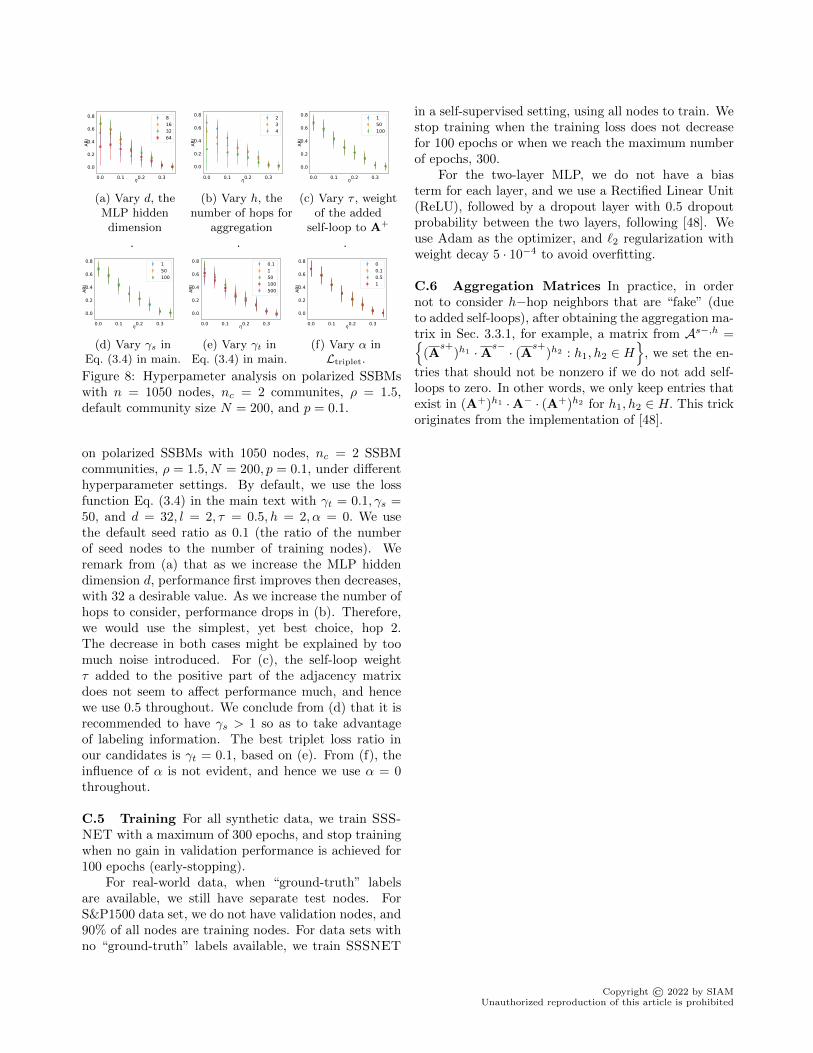
(f) Vary α inLtriplet.

Figure 8: Hyperpameter analysis on polarized SSBMswith n = 1050 nodes, nc = 2 communites, ρ = 1.5,default community size N = 200, and p = 0.1.

on polarized SSBMs with 1050 nodes, nc = 2 SSBMcommunities, ρ = 1.5, N = 200, p = 0.1, under differenthyperparameter settings. By default, we use the lossfunction Eq. (3.4) in the main text with γt = 0.1, γs =50, and d = 32, l = 2, τ = 0.5, h = 2, α = 0. We usethe default seed ratio as 0.1 (the ratio of the numberof seed nodes to the number of training nodes). Weremark from (a) that as we increase the MLP hiddendimension d, performance first improves then decreases,with 32 a desirable value. As we increase the number ofhops to consider, performance drops in (b). Therefore,we would use the simplest, yet best choice, hop 2.The decrease in both cases might be explained by toomuch noise introduced. For (c), the self-loop weightτ added to the positive part of the adjacency matrixdoes not seem to affect performance much, and hencewe use 0.5 throughout. We conclude from (d) that it isrecommended to have γs > 1 so as to take advantageof labeling information. The best triplet loss ratio inour candidates is γt = 0.1, based on (e). From (f), theinfluence of α is not evident, and hence we use α = 0throughout.

C.5 Training For all synthetic data, we train SSS-NET with a maximum of 300 epochs, and stop trainingwhen no gain in validation performance is achieved for100 epochs (early-stopping).

For real-world data, when “ground-truth” labelsare available, we still have separate test nodes. ForS&P1500 data set, we do not have validation nodes, and90% of all nodes are training nodes. For data sets withno “ground-truth” labels available, we train SSSNET

in a self-supervised setting, using all nodes to train. Westop training when the training loss does not decreasefor 100 epochs or when we reach the maximum numberof epochs, 300.

For the two-layer MLP, we do not have a biasterm for each layer, and we use a Rectified Linear Unit(ReLU), followed by a dropout layer with 0.5 dropoutprobability between the two layers, following [48]. Weuse Adam as the optimizer, and `2 regularization withweight decay 5 · 10−4 to avoid overfitting.

C.6 Aggregation Matrices In practice, in ordernot to consider h−hop neighbors that are “fake” (dueto added self-loops), after obtaining the aggregation ma-trix in Sec. 3.3.1, for example, a matrix from As−,h =

(As+

)h1 ·As− · (As+)h2 : h1, h2 ∈ H

, we set the en-

tries that should not be nonzero if we do not add self-loops to zero. In other words, we only keep entries thatexist in (A+)h1 ·A− · (A+)h2 for h1, h2 ∈ H. This trickoriginates from the implementation of [48].


sssnet: semi-supervised signed network clustering

Documents