stability and control of flight vehicle
DESCRIPTION
Overview on Stability and Control of an airplane.TRANSCRIPT

Stability and Control of Flight Vehicle
Uy-Loi LyDepartment of Aeronautics and Astronautics, Box 352400
University of WashingtonSeattle, WA 98195
September 29, 1997

i
c©Copyright 1997, by Uy-Loi Ly. All rights reserved.
No parts of this book may be photocopied or reproduced in any form without the written permission.

Contents
Glossary viii
1 Introduction 11.1 Lift Equation . . . . . . . . . . . . . . . . . . . . . . . . . . . . . . . . . . . . . . . . . 21.2 Drag Equation . . . . . . . . . . . . . . . . . . . . . . . . . . . . . . . . . . . . . . . . 31.3 Pitching Moment Equation . . . . . . . . . . . . . . . . . . . . . . . . . . . . . . . . . . 4
2 Linear Algebra and Matrices 52.1 Operations . . . . . . . . . . . . . . . . . . . . . . . . . . . . . . . . . . . . . . . . . . 72.2 Matrix Functions . . . . . . . . . . . . . . . . . . . . . . . . . . . . . . . . . . . . . . . 82.3 Linear Ordinary Differential Equations . . . . . . . . . . . . . . . . . . . . . . . . . . . 112.4 Laplace Transform . . . . . . . . . . . . . . . . . . . . . . . . . . . . . . . . . . . . . . 132.5 Stability . . . . . . . . . . . . . . . . . . . . . . . . . . . . . . . . . . . . . . . . . . . 162.6 Example . . . . . . . . . . . . . . . . . . . . . . . . . . . . . . . . . . . . . . . . . . . 17
2.6.1 Laplace method . . . . . . . . . . . . . . . . . . . . . . . . . . . . . . . . . . . 172.6.2 Time-domain method . . . . . . . . . . . . . . . . . . . . . . . . . . . . . . . . 182.6.3 Numerical integration method (via MATLAB) . . . . . . . . . . . . . . . . . . . . 20
3 Principles of Static and Dynamic Stability 23
4 Static Longitudinal Stability 274.1 Notations and Sign Conventions . . . . . . . . . . . . . . . . . . . . . . . . . . . . . . . 274.2 Stick-Fixed Stability . . . . . . . . . . . . . . . . . . . . . . . . . . . . . . . . . . . . . 274.3 Stick-Free Stability . . . . . . . . . . . . . . . . . . . . . . . . . . . . . . . . . . . . . . 344.4 Other Influences on the Longitudinal Stability . . . . . . . . . . . . . . . . . . . . . . . . 39
4.4.1 Influence of Wing Flaps . . . . . . . . . . . . . . . . . . . . . . . . . . . . . . . 394.4.2 Influence of the Propulsive System . . . . . . . . . . . . . . . . . . . . . . . . . 404.4.3 Influence of Fuselage and Nacelles . . . . . . . . . . . . . . . . . . . . . . . . . 424.4.4 Effect of Airplane Flexibility . . . . . . . . . . . . . . . . . . . . . . . . . . . . 424.4.5 Influence of Ground Effect . . . . . . . . . . . . . . . . . . . . . . . . . . . . . . 43
5 Static Longitudinal Control 455.1 Longitudinal Trim Conditions with Elevator Control . . . . . . . . . . . . . . . . . . . . . 45
5.1.1 Determination of Elevator Angle for a New Trim Angle of Attack . . . . . . . . . . 485.1.2 Longitudinal Control Position as a Function of Lift Coefficient . . . . . . . . . . . 48
ii
CONTENTS iii
5.2 Control Stick Forces . . . . . . . . . . . . . . . . . . . . . . . . . . . . . . . . . . . . . 505.2.1 Stick Force for a Stabilator . . . . . . . . . . . . . . . . . . . . . . . . . . . . . . 515.2.2 Stick Force for a Stabilizer-Elevator Configuration . . . . . . . . . . . . . . . . . 53
5.3 Steady Maneuver . . . . . . . . . . . . . . . . . . . . . . . . . . . . . . . . . . . . . . . 555.3.1 Horizontal Stabilizer-Elevator Configuration: Elevator per g . . . . . . . . . . . . 565.3.2 Horizontal Stabilator Configuration: Elevator per g . . . . . . . . . . . . . . . . . 585.3.3 Stabilizer-Elevator Configuration: Stick Force per g . . . . . . . . . . . . . . . . . 585.3.4 Stabilator Configuration: Stick Force per g . . . . . . . . . . . . . . . . . . . . . 59
6 Lateral Static Stability and Control 616.1 Yawing and Rolling Moment Equations . . . . . . . . . . . . . . . . . . . . . . . . . . . 61
6.1.1 Contributions to the Yawing Moment . . . . . . . . . . . . . . . . . . . . . . . . 636.1.2 Contributions to the Rolling Moment . . . . . . . . . . . . . . . . . . . . . . . . 67
6.2 Directional Stability (Weathercock Stability) . . . . . . . . . . . . . . . . . . . . . . . . . 726.3 Directional Control . . . . . . . . . . . . . . . . . . . . . . . . . . . . . . . . . . . . . . 746.4 Roll Stability . . . . . . . . . . . . . . . . . . . . . . . . . . . . . . . . . . . . . . . . . 746.5 Roll Control . . . . . . . . . . . . . . . . . . . . . . . . . . . . . . . . . . . . . . . . . 74
7 Review of Rigid Body Dynamics 757.1 Force Equations . . . . . . . . . . . . . . . . . . . . . . . . . . . . . . . . . . . . . . . 787.2 Moment Equations . . . . . . . . . . . . . . . . . . . . . . . . . . . . . . . . . . . . . . 797.3 Euler’s Angles . . . . . . . . . . . . . . . . . . . . . . . . . . . . . . . . . . . . . . . . 79
8 Linearized Equations of Motion 858.1 Linearized Linear Acceleration Equations . . . . . . . . . . . . . . . . . . . . . . . . . . 858.2 Linearized Angular Acceleration Equations . . . . . . . . . . . . . . . . . . . . . . . . . 888.3 Linearized Euler’s Angle Equations . . . . . . . . . . . . . . . . . . . . . . . . . . . . . 908.4 Forces and Moments in terms of their Coefficient Derivatives . . . . . . . . . . . . . . . . 90
8.4.1 Lift Force L . . . . . . . . . . . . . . . . . . . . . . . . . . . . . . . . . . . . . 918.4.2 Drag Force D . . . . . . . . . . . . . . . . . . . . . . . . . . . . . . . . . . . . 928.4.3 Side-Force Y . . . . . . . . . . . . . . . . . . . . . . . . . . . . . . . . . . . . . 938.4.4 Thrust Force T . . . . . . . . . . . . . . . . . . . . . . . . . . . . . . . . . . . . 938.4.5 Pitching Moment M . . . . . . . . . . . . . . . . . . . . . . . . . . . . . . . . . 948.4.6 Yawing Moment N . . . . . . . . . . . . . . . . . . . . . . . . . . . . . . . . . 948.4.7 Rolling Moment L . . . . . . . . . . . . . . . . . . . . . . . . . . . . . . . . . . 95
9 Linearized Longitudinal Equations of Motion 979.1 Phugoid-Mode Approximation . . . . . . . . . . . . . . . . . . . . . . . . . . . . . . . . 1039.2 Short-Period Approximation . . . . . . . . . . . . . . . . . . . . . . . . . . . . . . . . . 105
10 Linearized Lateral Equations of Motion 109
11 Flight Vehicle Models 11711.1 Generic F-15 Model Data (Subsonic) . . . . . . . . . . . . . . . . . . . . . . . . . . . . 11711.2 Generic F-15 Model Data (Supersonic) . . . . . . . . . . . . . . . . . . . . . . . . . . . 121

List of Figures
1.1 Motion in the Longitudinal Axis . . . . . . . . . . . . . . . . . . . . . . . . . . . . . . . 2
3.1 Three Possible Cases of Static Stability . . . . . . . . . . . . . . . . . . . . . . . . . . . 243.2 Three Possible Cases of Dynamic Stability . . . . . . . . . . . . . . . . . . . . . . . . . 25
4.1 Moments about the Center of Gravity of the Airplane . . . . . . . . . . . . . . . . . . . . 284.2 Definition of Aircraft Variables in Flight Mechanics . . . . . . . . . . . . . . . . . . . . . 284.3 Forces and Moments Applied to a Wing-Tail Configuration . . . . . . . . . . . . . . . . . 284.4 Moment Coefficient CMcg versus α . . . . . . . . . . . . . . . . . . . . . . . . . . . . . . 304.5 Calculation of Wing Aerodynamic Center . . . . . . . . . . . . . . . . . . . . . . . . . . 334.6 Horizontal Tail Configurations . . . . . . . . . . . . . . . . . . . . . . . . . . . . . . . . 344.7 Forces on a Propeller . . . . . . . . . . . . . . . . . . . . . . . . . . . . . . . . . . . . . 40
4.8 Propeller Normal Force Coefficient CNpα=
∂CNblade∂α
f (T ) . . . . . . . . . . . . . . . . . . 414.9 K f as a Function of the Position of the Wing c/4 Root Chord . . . . . . . . . . . . . . . . 42
5.1 How to Change Airplane Trim Angle of Attack . . . . . . . . . . . . . . . . . . . . . . . 465.2 Tail Lift Coefficient vs Tail Angle of Attack . . . . . . . . . . . . . . . . . . . . . . . . . 465.3 Tail Lift Coefficient vs Elevator Deflection . . . . . . . . . . . . . . . . . . . . . . . . . . 475.4 Determination of Stick-Fixed Neutral Point from Flight Test . . . . . . . . . . . . . . . . 505.5 Longitudinal Control Stick to Stabilator . . . . . . . . . . . . . . . . . . . . . . . . . . . 505.6 Stick Force versus Velocity Curve . . . . . . . . . . . . . . . . . . . . . . . . . . . . . . 53
6.1 Definition of the Lateral Directional Motion of an Airplane . . . . . . . . . . . . . . . . . 626.2 Effect of Sweepback on Total Lift and Rolling Moment to Sideslip . . . . . . . . . . . . . 686.3 Effect of Wing Placement on the Rolling Moment to Sideslip . . . . . . . . . . . . . . . . 696.4 Airplane with a Positive Sideslip . . . . . . . . . . . . . . . . . . . . . . . . . . . . . . . 73
7.1 Motion of a Rigid Body . . . . . . . . . . . . . . . . . . . . . . . . . . . . . . . . . . . 767.2 Euler’s Angle Definition . . . . . . . . . . . . . . . . . . . . . . . . . . . . . . . . . . . 80
8.1 Definition of Angle of Attack α and Sideslip β . . . . . . . . . . . . . . . . . . . . . . . 858.2 X and Z -Force Components in terms of L , D and T . . . . . . . . . . . . . . . . . . . . 87
9.1 Longitudinal Aircraft Responses to a 1-deg Elevator Impulsive Input . . . . . . . . . . . . 1049.2 Short-Period Approximation Model to a 1-deg Elevator Impulse Input . . . . . . . . . . . 107
10.1 Lateral Responses to a 1-deg Aileron Impulse Input . . . . . . . . . . . . . . . . . . . . . 115
iv

LIST OF FIGURES v
10.2 Lateral Responses to a 1-deg Rudder Impulse Input . . . . . . . . . . . . . . . . . . . . . 116

List of Tables
2.1 Laplace Transforms of Some Common Functions . . . . . . . . . . . . . . . . . . . . . . 13
vi

vii
viii Glossary
Glossary
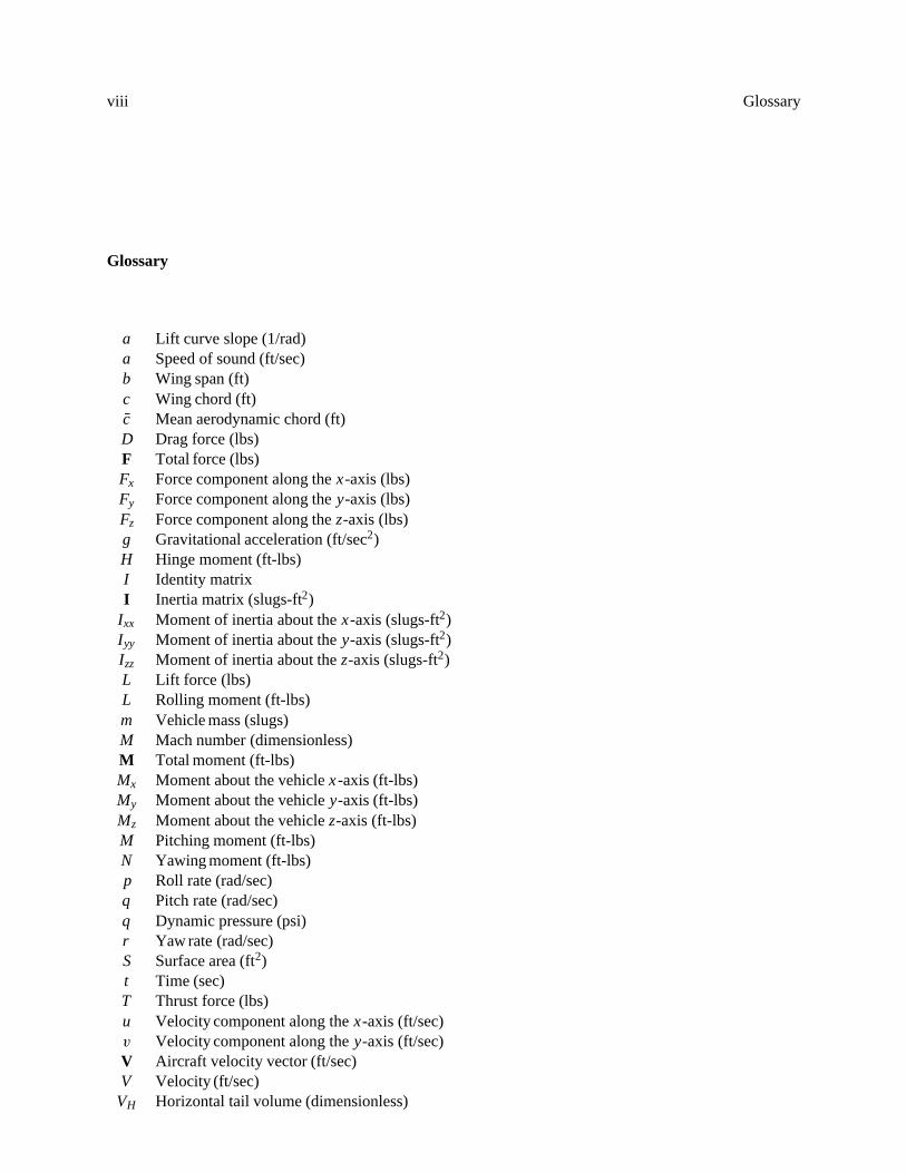
a Lift curve slope (1/rad)a Speed of sound (ft/sec)b Wing span (ft)c Wing chord (ft)c Mean aerodynamic chord (ft)D Drag force (lbs)F Total force (lbs)Fx Force component along the x-axis (lbs)Fy Force component along the y-axis (lbs)Fz Force component along the z-axis (lbs)g Gravitational acceleration (ft/sec2)H Hinge moment (ft-lbs)I Identity matrixI Inertia matrix (slugs-ft2)
Ixx Moment of inertia about the x-axis (slugs-ft2)Iyy Moment of inertia about the y-axis (slugs-ft2)Izz Moment of inertia about the z-axis (slugs-ft2)L Lift force (lbs)L Rolling moment (ft-lbs)m Vehicle mass (slugs)M Mach number (dimensionless)M Total moment (ft-lbs)Mx Moment about the vehicle x -axis (ft-lbs)My Moment about the vehicle y-axis (ft-lbs)Mz Moment about the vehicle z-axis (ft-lbs)M Pitching moment (ft-lbs)N Yawing moment (ft-lbs)p Roll rate (rad/sec)q Pitch rate (rad/sec)q Dynamic pressure (psi)r Yaw rate (rad/sec)S Surface area (ft2)t Time (sec)T Thrust force (lbs)u Velocity component along the x-axis (ft/sec)v Velocity component along the y-axis (ft/sec)V Aircraft velocity vector (ft/sec)V Velocity (ft/sec)
VH Horizontal tail volume (dimensionless)
Glossary ix
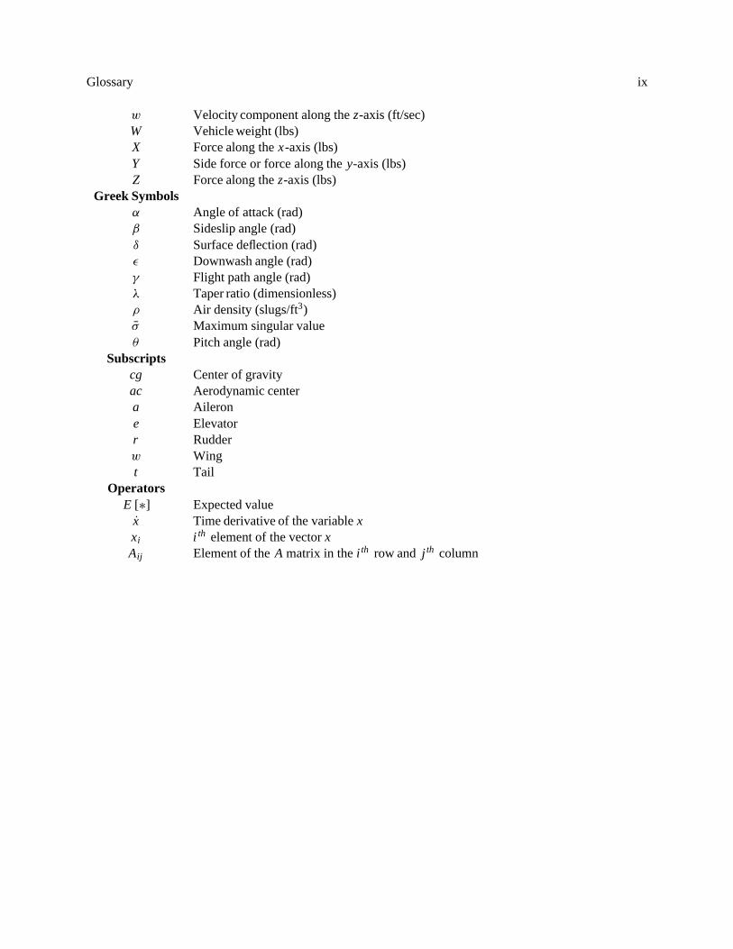
w Velocity component along the z-axis (ft/sec)W Vehicle weight (lbs)X Force along the x-axis (lbs)Y Side force or force along the y-axis (lbs)Z Force along the z-axis (lbs)
Greek Symbolsα Angle of attack (rad)β Sideslip angle (rad)δ Surface deflection (rad)ε Downwash angle (rad)γ Flight path angle (rad)λ Taper ratio (dimensionless)ρ Air density (slugs/ft3)σ Maximum singular valueθ Pitch angle (rad)
Subscriptscg Center of gravityac Aerodynamic centera Ailerone Elevatorr Rudderw Wingt Tail
OperatorsE [∗] Expected value
x Time derivative of the variable xxi i th element of the vector xAij Element of the A matrix in the i th row and j th column

x Glossary
Chapter 1
Introduction
The objective of this course is to develop fundamental understanding on the subject of stability, control andflight mechanics. Familiarities with the basic components in aerodynamics of wing and airfoil section areexpected; namely definition of lift, drag and moment of wing section, and physical parameters that governthese aerodynamic forces and moments suchas freestream velocity,density, Mach number, Reynold number,shape of the airfoil (camber, thickness, aerodynamic center), wing configuration (wing span, reference area,mean aerodynamic chord, taper ratio, sweep angle), angle of attack, dynamic pressure, etc· · ·. It is not theintent of this course to provide all these relevant background materials, although we will define the relevantones as we encounter them in our problem formulation.
Starting from known forces and moments generated on a given wing, fuselage and tail configuration, wewill develop airplane static and dynamic model to study its behavior under different flight regimes. Massproperties, wing, fuselage and tail configurations of the airplane are therefore assumed known and givena-priori. Concepts of static stability and dynamic stability are introduced in this course. General equationsof motion for a rigid-body airplane are derived. Basic motions of the aircraft separated into longitudinal andlateral modes are discussed in details. Effects of aerodynamic stability derivatives upon the behaviour of theperturbed equations of motions are studied. Flying qualities of the uncontrolled airplane can subsequentlybe assessed. Analysis of the airplane dynamic responses to initial changes in its basic motion variables (e.g.angle of attack, pitch attitude, roll angle, sideslip, etc· · ·), tocontrol inputs and external gust inputs iscoveredusing Laplace transform techniques and time simulation. It is expected that students are familiar somewhatwith the use of the MATLAB software for analysis.
There is an extensive number of references that cover the subject of aircraft stability, control and flightmechanics. Listed below are some that provide good reference materials:
1. John D. Anderson, Jr., Introduction to Flight, Third Edition, McGraw-Hill Book Company, 1989.
2. Arthur W. Babister, Aircraft Dynamic Stability and Response, First Edition, Pergamon Press, 1980.
3. John H. Blakelock, Automatic Control of Aircraft and Missiles, Second Edition, John Wiley & Sons,Inc., 1991.
4. Bernard Etkin, Dynamics of Flight: Stability and Control,, Second Edition, John Wiley & Sons, Inc.,1982.
5. Barnes W. McCormick, Aerodynamics, Aeronautics, and Flight Mechanics, John Wiley & Sons, Inc.,1979.
1
2 CHAPTER 1. INTRODUCTION
α
x-body axis
z-body axis
mg
γθ
L (lift)
D (drag)
VT (thrust)
My
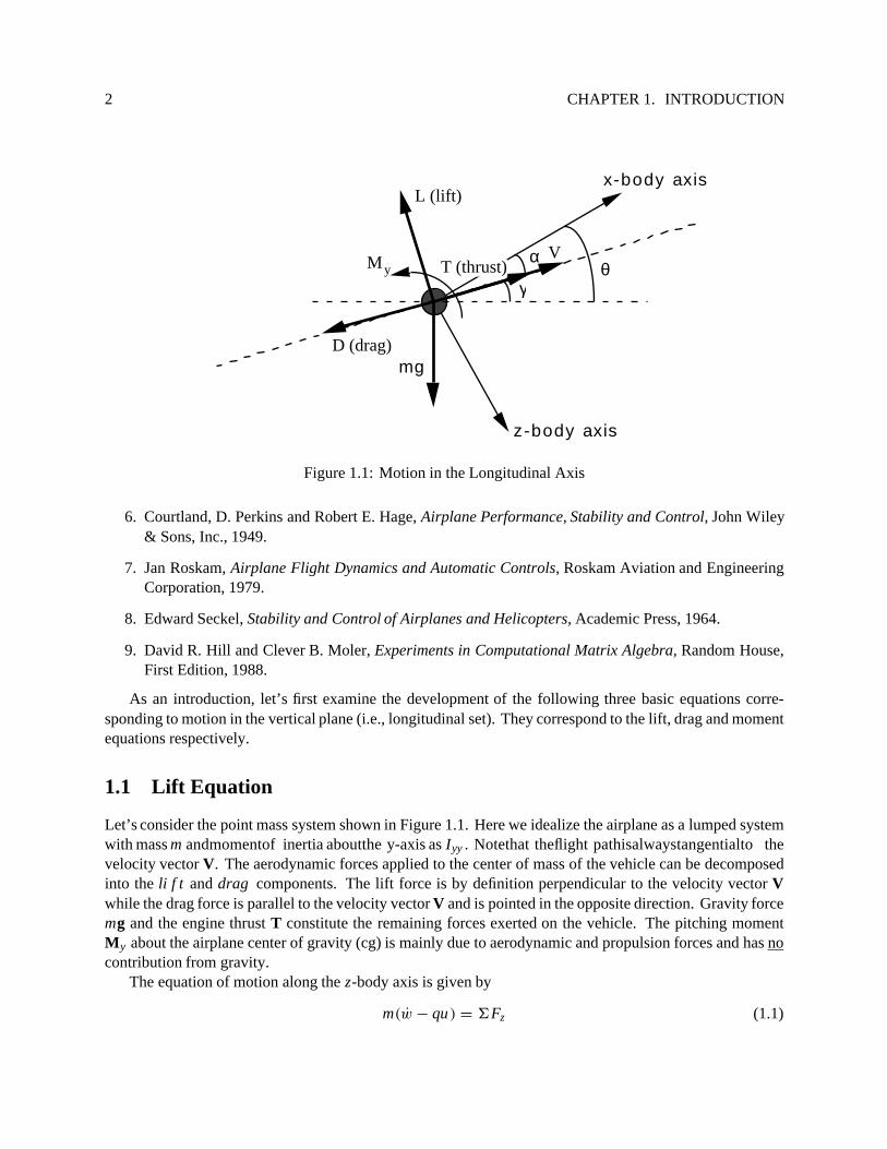
Figure 1.1: Motion in the Longitudinal Axis
6. Courtland, D. Perkins and Robert E. Hage, Airplane Performance, Stability and Control, John Wiley& Sons, Inc., 1949.
7. Jan Roskam, Airplane Flight Dynamics and Automatic Controls, Roskam Aviation and EngineeringCorporation, 1979.
8. Edward Seckel, Stability and Control of Airplanes and Helicopters, Academic Press, 1964.
9. David R. Hill and Clever B. Moler, Experiments in Computational Matrix Algebra, Random House,First Edition, 1988.
As an introduction, let’s first examine the development of the following three basic equations corre-sponding to motion in the vertical plane (i.e., longitudinal set). They correspond to the lift, drag and momentequations respectively.
1.1 Lift Equation
Let’s consider the point mass system shown in Figure 1.1. Here we idealize the airplane as a lumped systemwith mass m andmomentof inertia aboutthe y-axis as Iyy . Notethat theflight pathisalwaystangentialto thevelocity vector V. The aerodynamic forces applied to the center of mass of the vehicle can be decomposedinto the li f t and drag components. The lift force is by definition perpendicular to the velocity vector Vwhile the drag force is parallel to the velocity vector V and is pointed in the opposite direction. Gravity forcemg and the engine thrust T constitute the remaining forces exerted on the vehicle. The pitching momentMy about the airplane center of gravity (cg) is mainly due to aerodynamic and propulsion forces and has nocontribution from gravity.
The equation of motion along the z-body axis is given by
m(w − qu ) = 6Fz (1.1)

1.2. DRAG EQUATION 3
where u is the component of velocity along the x-body axis of the vehicle, w is the component along thez-body axis and q is the pitch angular velocity about the y-body axis. From Figure 1.1, we have
6Fz = Fz(aerodynamics ) + Fz(propulsion ) + Fz(gra vity ) (1.2)
whereFz(aerodynamics ) + Fz(propulsion ) = −Lcos α + (T − D)sin α
∼= −L + (T − D)α (for small α)(1.3)
Fz(gra vity ) = mgcos θ∼= W (for small θ)
(1.4)
where W is the weight of the vehicle. Let’s rewrite the velocity component w as w = Vsin α and thus,
w = Vsin α + V αcosα∼= Vα + V α (for small α)
(1.5)
Generally, we notice that the product V α is much smaller than V α. Hence, equation (1.5) is simplified to
w = V α (1.6)
Combining equations (1.1), (1.2), (1.3), (1.4) and (1.6), we obtain the following equation in the z-bodydirection,
m(V α − θV ) = −L + (T − D)α + W (1.7)
since q = θ and u = Vcos α ∼= V . Usually, the terms T − D and α are small and hence we can drop theproduct (T − D)α in the above equation. Thus,
mV (α − θ ) = W − L (1.8)
Note that the flight path angle is defined as γ = θ − α, equation (1.8) can be rewritten as
mV γ = L − W (1.9)
Thus, change in flight path occurs when L − W 6= 0 and the correspondingflight trajectory would be curved.For a constant flight path angle (i.e. γ = γo =constant), we must have γ = 0 and L − W = 0.
1.2 Drag Equation
Again we refer to Figure 1.1, the equation of motion in the x-body direction is as follows,
m(u + qw) = 6Fx (1.10)
since we are limited to motion in the vertical plane only. The force components in the x-body direction areonly consisted of 6Fx = Fx(aerodynamics ) + Fx(propulsion ) + Fx(gravity ). Each of these components can againbe written in terms of the lift L , drag D, thrust T and gravity W forces according to Figure 1.1. Namely,
Fx(aerodynamics ) + Fx(propulsion ) = Lsin α + (T − D)cosα∼= Lα + (T − D) (for small α)
(1.11)

4 CHAPTER 1. INTRODUCTION
andFx(gra vity ) = −mgsin θ ≈ −Wθ (for small θ) (1.12)
Furthermore, the velocity component u can be rewritten as u = Vcos α. Hence, its time derivative becomes
u = Vcos α − V αsin α
= V − V αα (for small α)(1.13)
Substituting equations (1.11), (1.12) and (1.13) into equation (1.10), we obtain the following
mV + mα(V θ − V α) = T − D + (L − W)α − W (θ − α) (1.14)
or,mV + Wγ = T − D + α(L − W − mV γ ) (1.15)
Using equation (1.9), equation (1.15) is simplified to
mV + Wγ = T − D (1.16)
Thus from the above equation with excess thrust, i.e. (T − D) > 0, one can have different flight trajectories:
• Positive flight path angle γ > 0 with V = 0. This results in a steady (nonaccelerated) climb.
• Positive acceleration V > 0 with γ = 0. This corresponds to an accelerated straight and level flight.
• Positive acceleration V > 0 and γ > 0. The vehicle speed increases while climbing.
1.3 Pitching Moment Equation
Finally, we derive the pitching moment equation for the vehicle shown in Figure 1.1,
Iyy θ = My(aerodynamics ) + My(propulsion ) (1.17)
Notice that by definition, gravity would have no moment contribution to the pitching moment equation whenit is taken about the vehicle center of gravity. Detailed description of the moments produced by aerodynamicand propulsive forces will be given later when we examine issues related to longitudinal static stability. Itsuffices to say that static longitudinal stability is predominantly governed by the behaviour of the pitchingmoment as the vehicle is perturbed from its equilibrium state.
Chapter 2
Linear Algebra and Matrices
We deal with 3 classes of numbers: scalars, single numbers without association; vectors, one dimensionalgroupings of scalars (one column, several rows, or one row, several columns); and finally, matrices, whichfor us will be 2-dimensional (rows and columns).
A vector can be either a row vector such as
Es = [s1 s2 · · · sn] ,
or a column vector, such as
Es =
s1
s2...
sn
.
Column vectors are vastly more common. Implied with every vector is a basis (often a physical basis) towhich each component refers. For instance, the position vector Er given by
Er = x x + y y + zz
is represented with respect to a cartesian basis [x, y, z]. Usually the shorthand [x, y, z] is used.MATLAB will use both row and column vectors. However column vectors are more often used in its
functions. Note that in the example below, the first entry in boldface is what the user types, and the secondcorresponds to MATLAB’sresponse.
• A = [1. 2. 3. 4.]A =1 2 3 4
• A = [1. 2. 3. 4.]’A =1234
5

6 CHAPTER 2. LINEAR ALGEBRA AND MATRICES
• A = [1;2;3;4]A =1234
• A = [1234]A=1234
A matrix can be thought of as a row of column vectors, or a column of row vectors,
A =[a1 a2 · · · am
]=
a1
a2...
an
=
a11 a12 · · · a1m
a21 a22 · · · a2m...
.... . .
...
an1 an2 · · · anm
.
One can think of matrices as having a basis in the form of dyadic products of basis vectors, though that willbe beyond the scope of this course.
Entry of a matrix in MATLAB is fairly straightforward. It follows along the lines of a vector, butremember that the entries are processed in row fashion:
• A = [1 2 3 4;5 6 7 8;9 10 11 12]A=1 2 3 45 6 7 89 10 11 12
• A = [1 2 3 45 6 7 89 10 11 12]A=1 2 3 45 6 7 89 10 11 12
• B = [A [0 1;2 3;4 5]; 6 5 4 3 2 1; 3 4 5 6 7 8; 1 3 5 7 9 11]B =1 2 3 4 0 15 6 7 8 2 3

2.1. OPERATIONS 7
9 10 11 12 4 56 5 4 3 2 13 4 5 6 7 81 3 5 7 9 11
MATLAB also has facilities for creating simple matrices such as a matrix of zeros or the identity matrix.For example, the matrix function zeros(n,m) will create a zero matrix of dimension n by m, and eye(n) willcreate an identity matrix of dimension n.
2.1 Operations
Addition and multiplication not only need to be defined for within a certain class, but between classes. Forexample, multiplication of vectors and matrices by a scalar,
α ∗ Ev =
αs1
αs2...
αsn
; α ∗ M =
αa11 αa12 · · · αa1m
αa21 αa22 · · · αa2m...
.... . .
...
αan1 αan2 · · · αanm
.
In MATLAB, however, you can add a scalar to every element in a vector or matrix without any specialnotation.
Adding two vectors occurs on an element by element level. Implied in all of this is that the basis of thetwo vectors is the same:
Ev + Eu = [ v1 v2 · · · vn ] + [ u1 u2 · · · un ]
= [ v1 + u1 v2 + u2 · · · vn + un ]
Multiplication of two vectors is mostly defined in terms of the dot product. While much mathematicaltheory has been expounded on inner product spaces and such, the only item we need know here is the innerproduct of two vectors expressed in a Cartesian coordinate frame,
Ev · Eu = [ v1 v2 · · · vn ] ∗
u1
u2...
un
= v1u1 + v2u2 + · · · + vnun
Multiplying a vector by a matrix is equivalent to transforming the vector. In components, the product ofa matrix and a vector is given by
A ∗ Ev =
a11 a12 · · · a1m
a21 a22 · · · a2m...
.... . .
...
an1 an2 · · · anm
∗
v1
v2...
vm
=
a11v1 + a12v2 + · · · + a1mvm
a21v1 + a22v2 + · · · + a2mvm...
an1v1 + an2v2 + · · · + anmvm

8 CHAPTER 2. LINEAR ALGEBRA AND MATRICES
Of course, the number of columns of A must match the number of rows of Ev.Adding two matrices of the same dimensions would occur on an element by element basis,
A + B =
a11 a12 · · · a1m
a21 a22 · · · a2m...
.... . .
...
an1 an2 · · · anm
+
b11 b12 · · · b1m
b21 b22 · · · b2m...
.... . .
...
bn1 bn2 · · · bnm
=
a11 + b11 a12 + b12 · · · a1m + b1m
a21 + b21 a22 + b22 · · · a2m + b2m...
.... . .
...
an1 + bn1 an2 + bn2 · · · anm + bnm
Multiplying two matrices can be thought of as a series of transformations on the column vectors of themultiplicand. The number of columns of the left matrix must be equal to the number of rows of the rightmatrix (left and right are significant since multiplication is not commutative for matrices in general).
A ∗ B =
a11 a12 · · · a1m
a21 a22 · · · a2m...
.... . .
...
an1 an2 · · · anm
∗[b1 b2 · · · bp
]
=
a11b11 + a12b21 + · · · + a1mbm1
a21b11 + a22b21 + · · · + a2mbm1...
an1b11 + an2b21 + · · · + anm bm1
a11b12 + a12b22 + · · · + a1mbm2
a21b12 + a22b22 + · · · + a2mbm2...
an1b12 + an2b22 + · · · + anm bm2
· · ·
· · ·. . .
...
Thestandardsymbols: +, -, *, and/willhandle all legal operationsbetween scalars, vectors, andmatricesin MATLAB without any further special notation.
2.2 Matrix Functions
The convenience of matrix notation is in the representation of a group of linear equations. For example, thefollowing set of equations,
a11x1 +a12x2 +· · · +a1n xn = b1
a21x1 +a22x2 +· · · +a2n xn = b2...
...
an1x1 +an2x2 +· · · +ann xn = bn
can be represented compactly by the relation
AEx = Eb.
Note that we have the number of knowns Eb equal to the number of unknowns Ex here. How does one solvethis? The most simplistic (and computationally efficient) method is to apply a succession of transformations

2.2. MATRIX FUNCTIONS 9
to the above system to eliminate values of A below the diagonal. Suppose that a11 is nonzero then one canmultiply the first equation by a21/a11 and subtracts it from the second equation. The first term in the secondequation would be eliminated,
a11x1 + a12x2 + · · · + a1nxn = b1
0 + (a22 − a12a21/a11)x2 + · · · + (a2n − a1na21/a11)xn = b2 − b1a21/a11... +
... +... +
... =...
an1x1 + an2x2 + · · · + ann xn = bn
Suppose that the procedure were repeated for all the other rows, resulting in the removal of the coefficientof x1 in these equations. The same procedure is now applied to all coefficients of x2 for all rows below thesecond row. What one would eventually have is the upper triangular system. (In general, the aij ’s and b j ’sare NOT the same as the original matrix entries aij and b j , respectively).
a11x1 + a12x2 + · · · + a1n xn = b1
0 + a22x2 + · · · + a2n xn = b2 − b1a21/a11
0 + 0 + · · · + · · · = · · ·... +
... +... +
... =...
0 + 0 + · · · + ann xn = bn
All values of aij below the diagonal are zero. This matrixalso has the interesting propertythat the product ofthe diagonal terms is equal to the determinant. This substantiates the argument that it costs about as much tosolve a linear system as it does to solve for a determinant. Note that one can now solve xn = bn/ann . Onceyou have xn, you can substitute it into the next equation up and solve for xn−1. This continues until one getsto x1 (or until some diagonal term akk is zero). Note that if a diagonal term is zero, then the determinant isalso zero and the system matrix A is called singular .
The above method is often called the method of Gaussian elimination with back substitution. MATLABimplements a method very much similar to the above for solving a system of linear equations. You can,however, obtain an answer from MATLAB with very little effort by just typing the commandx = A \ b
In a similarvein to whatis notedabove, the determinant is computedwith the followingcommand syntaxdet(A).
The inverse can also be computed in a method similar to that above. If one solves for a succession ofvectors Exi (i = 1, n), each one with
Eb1 =
10...
0
; Eb2 =
01...
0
; · · · Ebn =
00...
1
;
thenthematrixcomposingofthecolumnvectors[ Ex1, · · · Exn]wouldbethematrixinverseof A. In MATLAB,computation of the matrix inverse is invoked by the command inv(A).
Itisoftennecessarytocomputeadeterminantoraninverseinsomethingresemblingaclosedform(whichwill be seen in the calculation of eigenvalues). Thus, one introduces the expansion by minors method. A

10 CHAPTER 2. LINEAR ALGEBRA AND MATRICES
minor Mij (A) of a matrix A is the determinant of the matrix A without its i th row and its j th column.
A =
a11 a12 a13 · · · a1n
a21 a22 a23 · · · a2n
a31 a32 a33 · · · a3n...
......
. . ....
an1 an2 an3 · · · ann
M12(A) = det
a21 a23 · · · a2n
a31 a33 · · · a3n...
.... . .
...
an1 an3 · · · ann
A determinant is formed from expanding by minors along an arbitrary row i or column j of a matrix:
By Row i : det (A) =n∑
j=1
aij Mij (A)(−1)i+ j
By Column j : det (A) =n∑
i=1
aij Mij (A)(−1)i+ j
Thus, what one has for an arbitrary matrix is a successionof expansions. First the matrix is broken down intoa series of minors to determine the determinant, then these minors may need be broken down further intotheir minors to find their determinants, and so on until one gets to a 1 × 1 matrix. For a scalar (i.e., 1 × 1)matrix,
A = [a11] H⇒ det (A) = a11.
It is also easy to evaluate the determinant of a 2 × 2 matrix by expanding along the first row,
A =
[a11 a12
a21 a22
]H⇒ det (A) = a11a22 − a12a21.
With a little more effort, one can get the determinant for the case of a 3 × 3 matrix. Here we expand alongthe first row.
A =
a11 a12 a13
a21 a22 a23
a31 a32 a33
H⇒ det (A) =a11a22a33 + a12a23a31 + a13a21a32
−a11a23a32 − a12a21a33 − a13a22a31
The inverse can also be found through expansion by minors. The recipe for this is a little more complicatedthan for the determinant. First one transposes the matrix, then each element aij gets replaced by the termMij (A)(−1)i+ j , where Mij (A) is the minor of A at i and j . Finally, each resulting new element is dividedby the determinant of the original matrix. For a 2 × 2 matrix, the inverse is
A =
[a11 a12
a21 a22
]H⇒ A−1 = inv(A) =
1
a11a22 − a12a21
[a22 −a12
−a21 a11
]

2.3. LINEAR ORDINARY DIFFERENTIAL EQUATIONS 11
The inverse of a 3 × 3 matrix is somewhat more complicated.
A =
a11 a12 a13
a21 a22 a23
a31 a32 a33
, A′ =
a11 a21 a31
a12 a22 a32
a13 a23 a33
H⇒ A−1 = inv(A) =1
det (A)
a22a33 − a32a23 a32a13 − a12a33 a12a23 − a13a22
a31a23 − a21a33 a11a33 − a31a13 a21a13 − a11a23
a21a32 − a31a22 a31a12 − a11a32 a11a22 − a21a12
Suppose that one applies this to the system
a11 a12 a13
a21 a22 a23
a31 a32 a33
∗
x1
x2
x3
=
b1
b2
b3
where the solution Ex is given byEx = A−1 ∗ Eb
If one goes through the algebra, the result obtained from the Cramer’s Rule will be
x1 =1
det (A)(b1a22a33 + b2a32a13 + b3a12a23 − b1a32a23 − b2a12a33 − b3a22a13)
... = (etc...)
This can be expressed more compactly as (with |A| being the shorthand notation for the determinant of A),
x1 =
∣∣∣∣∣∣∣
b1 a12 a13
b2 a22 a23
b3 a32 a33
∣∣∣∣∣∣∣det (A)
; x2 =
∣∣∣∣∣∣∣
a11 b1 a13
a21 b2 a23
a31 b3 a33
∣∣∣∣∣∣∣det (A)
; x3 =
∣∣∣∣∣∣∣
a11 a12 b1
a21 a22 b2
a31 a32 b3
∣∣∣∣∣∣∣det (A)
;
2.3 Linear Ordinary Differential Equations
Note that in this course we encounter mostly linear ordinary differential equations with constant coefficients.One can always find an integrating factor for the first-order equation
x + ax = f, x(0−) = xo
The term eat is an integrating factor for the above equation. Let’s multiply the above differential equationwith the integrating factor eat and collect terms, we have the following
d
dt
(eat x
)= eat f
Integrate both sides from 0− to time t ,
x = e−at[
xo +
∫ t
0−eaτ f (τ) dτ
]

12 CHAPTER 2. LINEAR ALGEBRA AND MATRICES
or,
x = xoe−at +
∫ t
0−e−a(t−τ ) f (τ) dτ
Theabovesolutioncontainsusuallyahomogeneoussolution(frominitialconditions)andaparticularsolution(from the forcing function f ). Note that solution for the particular part involves a convolution integral.
A second-order equation given by
x + ax + bx = f, x(0−) = xo, x(0−) = vo
can be written as a system of two first-order equations as follows. Let x1 = x and x2 = x , the above equationcan be re-written as [
x1
x2
]=
[0 1
−b −a
] [x1
x2
]+
[0f
]
In fact, the procedure leading to the solution of the above scalar first-order differential equation can be usedto derive the solution for a system of first-order differential equations. In the latter case, it would involve thematrix exponential (i.e., eAt ).
One could solve the above second-order system by first solving the homogeneous system whose solutionis usually of the form xh(t) = eλt where λ is the solution of the resulting characteristic equation. Theparticular solution from the non-homogenous part can be done either by means of a trial substitution orvariation of parameters. It turns out that the system of first-order differential equations is more amenable touse on the computer when expressed in a matrix state-space form. A formal way of modeling a dynamicsystem is by a set of state equations,
x = Ax + Bu (State equations)
y = Cx + Du (Output equations)
Theinput u isthe particular forcing function driving the system (i.e., u = f ). Refer back toour second-ordersystem with both (x and x ) as outputs. Then, in the above notation we have the following set of systemmatrices
A =
[0 1
−b −a
]B =
[01
]C =
[1 00 1
]D =
[00
]
Togenerate a time series responseof a linear time-invariant system inMATLAB, oneneeds to generatetheseA, B, C , and D matrices. Suppose that one creates a vector of time points where the system outputs are tobe computed with the MATLAB commandT =[0:0.1:10];This vector contains time points from 0 to 10 in steps of 0.1. The forcing function f (often referred to asthe control input) is a vector whose entries correspond to the value of this function at those time points. Togenerate the system time responses for the system matrices A, B, C, and D as defined above, at the timepoints defined in the vector T to the forcing function f , we can issue the following MATLAB commandY = lsim(A,B,C,D,f,T);The vector Y has 2 columns (each corresponding to an output) and 101 rows (each row corresponding to atime point).
2.4. LAPLACE TRANSFORM 13
2.4 Laplace Transform
Solving differential equations can also be done using the Laplace transform. We define
L( f (t)) =
∫ ∞
0−e−st f (t) dt = f (s)
The function e−at transforms as follows,
L(e−at ) =
∫ ∞
0−e−st e−at dt =
∫ ∞
0−e−(s+a)t dt = −
e−(s+a)t
s + a
∣∣∣∣∣
∞
0−
=1
s + a.
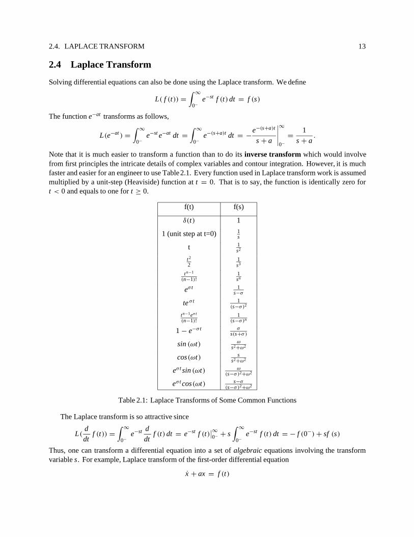
Note that it is much easier to transform a function than to do its inverse transform which would involvefrom first principles the intricate details of complex variables and contour integration. However, it is muchfaster and easier for an engineer to use Table2.1. Every function used in Laplace transform work is assumedmultiplied by a unit-step (Heaviside) function at t = 0. That is to say, the function is identically zero fort < 0 and equals to one for t ≥ 0.
f(t) f(s)
δ(t) 1
1 (unit step at t=0) 1s
t 1s2
t2
21s3
tn−1
(n−1)!1sn
eσ t 1s−σ
teσ t 1(s−σ)2
tn−1eσ t
(n−1)!1
(s−σ)n
1 − e−σ t σs(s+σ )
sin (ωt) ωs2+ω2
cos(ωt) ss2+ω2
eσ t sin (ωt) ω(s−σ)2+ω2
eσ t cos(ωt) s−σ(s−σ)2+ω2
Table 2.1: Laplace Transforms of Some Common Functions
The Laplace transform is so attractive since
L(d
dtf (t)) =
∫ ∞
0−e−st d
dtf (t) dt = e−st f (t)
∣∣∞0− + s
∫ ∞
0−e−st f (t) dt = − f (0−) + sf (s)
Thus, one can transform a differential equation into a set of algebraic equations involving the transformvariable s. For example, Laplace transform of the first-order differential equation
x + ax = f (t)
14 CHAPTER 2. LINEAR ALGEBRA AND MATRICES
issx (s) − x(0−) + ax (s) = f (s)
Solving for the variable x(s), we obtain the solution of the above differential equation in the Laplace domainas
x(s) =x(0−)
s + a+
f (s)
s + a
The first term of the sum corresponds to x(0−)e−at , the second is not solvable until one specifies f (t) (orf (s)). However, in general, the product of two Laplace transforms (in this case, f (s) and 1
s+a ) is equivalentto the convolution of their time-based functions. This particular case is equal to what has been previouslydemonstrated,
L−1{
f (s)
s + a
}=
∫ t
0−e−a(t−τ ) f (τ) dτ
Consider now the second-order differential equation
x + ax + bx = f
Applying Laplace transform to the above equation, we obtain
s2x(s) − sx (0−) − x(0−) + asx (s) − ax (0−) + bx (s) = f (s)
and, solving for the solution x(s)
x(s) =x(0−) + (s + a)x(0−) + f (s)
s2 + as + b
The homogeneous parts of this have equivalent time-domain functions that depend on the relation betweena and b. We distinguish three cases:
• b − a2/4 > 0
• b − a2/4 < 0
• b − a2/4 = 0
Case b − a2/4 > 0: The denominator can be written into the form s2 + 2σ s + σ 2 + ω2 which corresponds
to the time-domain functions e−σ tsin ωt and e−σ t cosωt where σ = −a/2 and ω =√
b − a2/4.Solutions to the homogeneous problem (i.e., to initial conditions x(0−)) can be obtained directly as
xh(t) = x(0−)e−at/2sin (
√b − a2/4 t)√
b − a2/4+
x(0−)e−at/2
{cos(
√b − a2/4 t) +
a
2√
b − a2/4sin (
√b − a2/4 t)
}
Use of Table 2.1 is not always possible with some more complicated forms. Usually one needs to breakdown a complicated polynomial fraction into simpler summands that are of the forms given in Table 2.1.

2.4. LAPLACE TRANSFORM 15
Suppose that the forcing function f (t) is a step input (applied at t=0) whose Laplace transform is simply1/s. We will derive the particular solution as an illustration to the partial fraction expansion methodology.The particular solution to the non-homogenous problem is
xp(s) =1
s(s2 + as + b)
The right-hand term can be decomposed into
1
s(s2 + as + b)=
u
s+
vs + w
s2 + as + b
with unknowns u, v and w. Expanding and matching the numerator term, we have
u(s2 + as + b) + vs2 + ws = 1
Since the coefficients of s2 and s must be zero, and that ub = 1, we have
u = 1/b , v = −1/b , w = −a/b
The particular solution is given by
xp(t) =1
b
[1 − e−at /2
{cos(
√b − a2/4 t) +
a
2√
b − a2/4sin (
√b − a2/4 t)
}]
Case b − a2/4 < 0: In this case, we have two distinct real roots to the equation s2 + as + b = 0. They are
given by
σ1 = −a/2 +
√a2/4 − b
σ2 = −a/2 −
√a2/4 − b
Solution to the homogenous problem is simply
xh(s) =x(0−) + (s + a)x(0−)
(s − σ1)(s − σ2)
or,
xh(t) =x(0−) + (σ1 + a)x(0−)
σ1 − σ2eσ1t +
x(0−) + (σ2 + a)x(0−)
σ2 − σ1eσ2t
Similarly, for the particular solution we have
xp(s) =1
s(s2 + as + b)
In partial fraction expansion
xp(s) =u
s+
v
s − σ1+
w
s − σ2
The unknowns u, v and w are determined from the following equation
u(s2 + as + b) + vs2 − vsσ2 + ws2 − wsσ1 = 1

16 CHAPTER 2. LINEAR ALGEBRA AND MATRICES
For the coefficients of s2 and s to vanish we must have u +v +w = 0 and ua −vσ2 −wσ1 = 0 with ub = 1.Thus, we have
u =1b
=1
σ1σ2, v =
1σ1(σ1 − σ2)
, w =1
σ2(σ2 − σ1)
Hence, the time-domain solution is
x p(t) =
(1
σ1σ2+
1σ1(σ1 − σ2)
eσ1t +1
σ2(σ2 − σ1)eσ2t
)H(t)
where H(t) corresponds to the Heaviside (step) function at t = 0.Case a2/4 = b: This case is similar to the previous case where
σ2 = σ1 = −a
2
Solution to the homogenous problem is simply
xh(s) =x(0−) + (s + a)x(0−)
(s − σ1)2
or,xh(t) = x(0−)teσ1t + x(0−)(1 − σ1t)eσ1t
Similarly, for the particular solution we have
x p(s) =1
s(s2 + as + b)=
u
s+
v
s − σ1+
w
(s − σ1)2
For the coefficients of s2 and s to vanish we must have u + v = 0 and −2σ1u − σ1v + w = 0 with u = 1/b.Hence,
u =1
σ 21
, v = −1
σ 21
, w =1
σ1
Or, in the time domain
xp(t) =
(1
σ 21
−1
σ 21
eσ1t +1σ1
teσ1t
)H (t)
InMATLAB,timeresponsesofasystemcanbeobtainedfromtheirLaplacetransformsdirectly. Responseof the outputs to an input U defined over the time points T can be obtained using the commandY = lsim(NUM,DEN,U,T);where the arguments NUM and DEN are arrays containing coefficients of the numerator and denominatorpolynomials in s arranged in descending powers of s.
2.5 Stability
Dynamicstability ischaracterizedbythe responseofasystem tononzeroinitialconditions. Initialconditionsare equivalent to an impulsive forcing function (i.e. Dirac delta function u(t) = δ(t)).
For a first-order system x + ax = 0 and x(0−) = xo, we have the homogeneous solution x(t) = xoe−at .It is simple to imagine that for a > 0, the response x(t) to initial conditions xo would tend toward zero (thusstable) as t → ∞. On the other hand, if a < 0 the response would tend to blow up.
For a second-order system x + ax + bx = 0, we have solutions of the form
2.6. EXAMPLE 17
• When a2/4 < b,x(t) = eσ t [usin ωt + vcosωt]
• When a2/4 > b,x(t) = ueσ1t + veσ2t
• When a2/4 = b,x(t) = ueσ t + vteσ t
In any case, the argument σ in the exponential function eσ t term must be less than or equal to zero. In thecase of a2/4 > b, both terms σ1 and σ2 must be less than or equal to zero. Otherwise, the solution will blowup as t → ∞. For σ equal to zero, then one has a neutrally stable system.
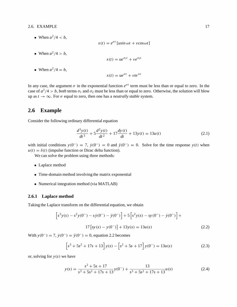
2.6 Example
Consider the following ordinary differential equation
d3y(t)
dt 3+ 5
d2y(t)
dt 2+ 17
dy (t)
dt+ 13y(t) = 13u(t) (2.1)
with initial conditions y(0−) = 7, y(0−) = 0 and y(0−) = 0. Solve for the time response y(t) whenu(t) = δ(t) (impulse function or Dirac delta function).
We can solve the problem using three methods:
• Laplace method
• Time-domain method involving the matrix exponential
• Numerical integration method (via MATLAB)
2.6.1 Laplace method
Taking the Laplace transform on the differential equation, we obtain
[s3y(s) − s2 y(0−) − s y(0−) − y(0−)
]+ 5
[s2 y(s) − sy (0−) − y(0−)
]+
17[sy (s) − y(0−)
]+ 13y(s) = 13u(s) (2.2)
With y(0−) = 7, y(0−) = y(0−) = 0, equation 2.2 becomes
[s3 + 5s2 + 17s + 13
]y(s) −
[s2 + 5s + 17
]y(0−) = 13u(s) (2.3)
or, solving for y(s) we have
y(s) =s2 + 5s + 17
s3 + 5s2 + 17s + 13y(0−) +
13s3 + 5s2 + 17s + 13
u(s) (2.4)

18 CHAPTER 2. LINEAR ALGEBRA AND MATRICES
For a unit impulse input u(t) = δ(t) or u(s) = 1 and y(0−) = 7, equation 2.4 becomes
y(s) = s2 + 5s + 17s3 + 5s2 + 17s + 13
7 + 13s3 + 5s2 + 17s + 13
1
= 7s2 + 35s + 132(s + 1)
[(s + 2)2 + 32]
(2.5)
Performing the partial fraction expansion on equation 2.5, we have
y(s) =R1
s + 1+
R2
s + 2 − j3+
R3
s + 2 + j3(2.6)
where
R1 =7s2 + 35s + 132[(s + 2)2 + 32
]∣∣∣∣∣s=−1
= 10.4
R2 =7s2 + 35s + 132
(s + 1) (s + 2 + j3)
∣∣∣∣∣s=−2+ j3
= −1.7 − j0.6
R3 =7s2 + 35s + 132
(s + 1) (s + 2 − j3)
∣∣∣∣∣s=−2− j3
= −1.7 + j0.6 = R2
where R2 is the complex conjugate of R2. Taking the inverse Laplace tranform on equation 2.6, we have
y(t) = R1e−t + R2e(−2+ j3)t + R2e(−2− j3)t (2.7)
or since ea+ jb = ea(cosb + jsinb ), we have
y(t) = 10.4e−t + e−2t (−1.7 − j0.6)(cos3t + jsin 3t) + (−1.7 + j0.6)(cos3t − jsin 3t) (2.8)
y(t) = 10.4e−t + 2e−2t (−1.7cos3t + 0.6sin 3t) (2.9)
2.6.2 Time-domain method
Let’s define x1(t) = y(t), x2(t) = y(t) and x3(t) = y(t), then clearly
x1(t) = x2(t) = y(t) (2.10)
x2(t) = x3(t) = y(t) (2.11)
and equation 2.1 can be re-written as
x3(t) + 5x3(t) + 17x2 + 13x1(t) = 13u(t) (2.12)
Combining equations 2.10-2.12 into a set of three first-order differential equations which can be expressedin a matrix equation,
x1(t)x2(t)x3(t)
=
0 1 00 0 1
−13 −17 −5
x1(t)x2(t)x3(t)
+
00
13
u(t) (2.13)
2.6. EXAMPLE 19
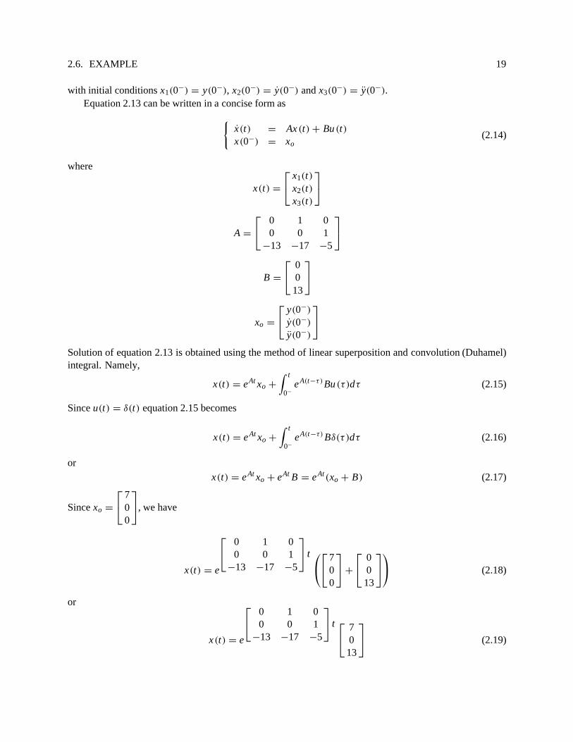
with initial conditions x1(0−) = y(0−), x2(0−) = y(0−) and x3(0−) = y(0−).Equation 2.13 can be written in a concise form as
{x(t) = Ax (t) + Bu (t)x(0−) = xo
(2.14)
where
x(t) =
x1(t)x2(t)x3(t)
A =
0 1 00 0 1
−13 −17 −5
B =
00
13
xo =
y(0−)
y(0−)
y(0−)
Solution of equation 2.13 is obtained using the method of linear superposition and convolution (Duhamel)integral. Namely,
x(t) = eAt xo +
∫ t
0−eA(t−τ )Bu (τ)dτ (2.15)
Since u(t) = δ(t) equation 2.15 becomes
x(t) = eAt xo +
∫ t
0−eA(t−τ) Bδ(τ )dτ (2.16)
orx(t) = eAt xo + eAt B = eAt(xo + B) (2.17)
Since xo =
700
, we have
x(t) = e
0 1 00 0 1
−13 −17 −5
t
700
+
00
13
(2.18)
or
x(t) = e
0 1 00 0 1
−13 −17 −5
t
70
13
(2.19)

20 CHAPTER 2. LINEAR ALGEBRA AND MATRICES
2.6.3 Numerical integration method (via MATLAB)
In MATLAB, the command lsim would perform numerical integration on the linear system{
x(t) = Ax (t) + Bu (t)y(t) = Cx (t) + Du(t)
(2.20)
for a given initial condition x(0−) = xo and an input function u(t) defined in the time interval 0 ≤ t ≤ tmax .More precisely, we can use the following set of MATLAB codes to perform the time responses of y(t)
for the linear system described in equation 2.20.
t=[0:.1:tmax];u= "some function of t" (e.g., u=ones(t) for a step input)y=lsim(A,B,C,D,u,t,xo)plot(t,y)
Below is a complete listing of the m-file for this example problem.
%Using the Laplace methodt=[0:.1:5];y=10.4*exp(-t)+2*exp(-2*t) .* (-1.7*cos(3*t)+0.6*sin(3*t));%Using the state-space methodA=[0,1,0;0,0,1;-13,-17,-5];B=[0;0;13];C=[1,0,0];D=0;xo=[7;0;0];[n,m]=size(t);%Solution from the exponential matrixyexp=[];for i=1:length(t)ti=t(i);ytemp= expm(A*ti)*(xo+B);yexp=[yexp;ytemp'];end%MATLAB command for solving time responses%For an impulse input the new initial condition becomes x(o+)=x(0-)+b% and the input u(t)=0 for t>0+xoplus=xo+B;u=zeros(n,m);ysim=lsim(A,B,C,D,u,t,xoplus);%Plot the responses for comparisonplot(t,y,'o',t,yexp)gridxlabel('Time (sec)')ylabel('y(t)')title('Exponential matrix method')pause%Plot the responses for comparisonplot(t,y,'o',t,ysim)grid

2.6. EXAMPLE 21
xlabel('Time (sec)')ylabel('y(t)')title('Laplace method')

22 CHAPTER 2. LINEAR ALGEBRA AND MATRICES

Chapter 3
Principles of Static and Dynamic Stability
In most design situation, static and dynamic stability analysis plays a significant role in the determination ofthe final airplane design configuration. The decision is based according to the requirements defined in FARPart 23 which states that
“the airplanemust besafely controllableand maneuverableduring — (1)take off; (2)climb;(3)levelflight; (4)dive; and(5)landing(poweron, off)(with wingflapsextendedandretracted)”
Stability of such a vehicle is also a major consideration in selecting a particular design configuration. Theairplane must be longitudinally, directionally and laterally stable for airworthiness and minimal pilot work-load. If the airplane turns out to have undesireable flying qualities, then some of these requirements mustsubsequently be met by the use of stability augmentation systems. This requires careful design of a controlsystem that feedbacks sensed aircraft motion variables to the appropriate control surfaces (e.g. elevator,aileron and rudder). The topic of feedback synthesis of flight control systems for stability augmentation andautopilot designs is the subject of AA-517 and a continuation in AA-518. In the present course, we willonly examine the fundamental behaviour of flight vehicle and its inherent flight characteristics without theinfluence of artificial feedback control.
The general notion of stability refers to the tendency of the vehicle to return to its original state ofequilibrium (e.g., trim point) when disturbed. There are basically two types of stability:
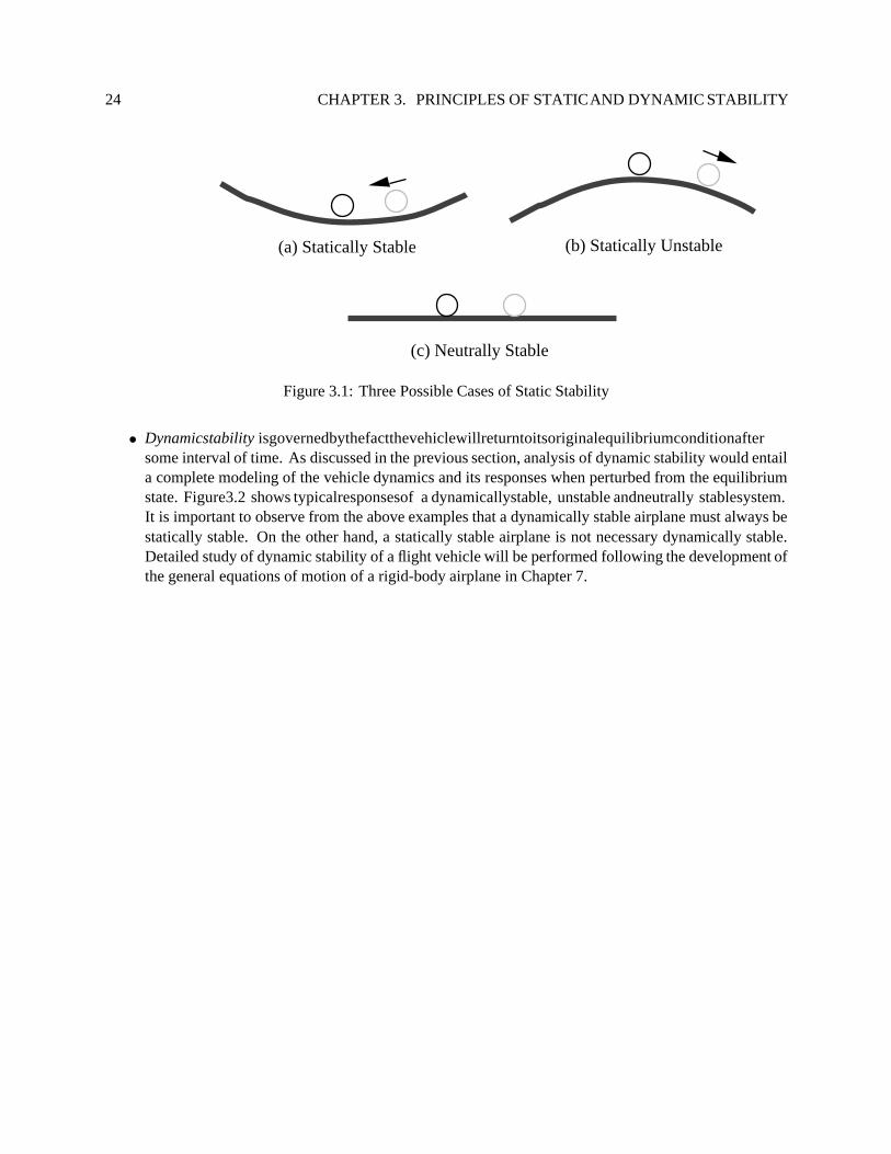
• Static stability refers to the tendency of an airplane under static conditions to return to its trimmedcondition. Clearly we assume that there exists an equilibrium point about which static stability isinvestigated. The evaluation of static stability involves purely static (i.e. steady-state) equations fromforce and moment balance applied to a vehicle disturbed from its equilibrium. Conditions for stabilityare governedby the directionof the forces andmoments thatwill restorethevehicletothe originaltrimstates. Figure 3.1 shows the three possible cases of static stability. Clearly, from these illustrations, wedetermine stability from the direction of the restoring force. In Figure 3.1 (a) component of the gravityforce tangential to the surface will bring the ball back to its original equilibrium point. However, instaticstability analysisthereisnomentionon how andwhen theballwillreturntoitsequilibriumpoint.For example, without the benefit of friction, the ball will oscillate back and forth about the equilibriumpointandthereforewillnever reachtheequilibriumstate. Totreatthisproblemconcerningthedynamicbehaviour of this ball rolling on a curved surface, one will need to first develop its equation of motionand then analyze the stability of its motion when released from a perturbed position. Stability of theball in motion is then determined by the phenomena of dynamic stability.
23
24 CHAPTER 3. PRINCIPLES OF STATICAND DYNAMIC STABILITY
(a) Statically Stable (b) Statically Unstable
(c) Neutrally Stable
Figure 3.1: Three Possible Cases of Static Stability
• Dynamicstability isgovernedbythefactthevehiclewillreturntoitsoriginalequilibriumconditionaftersome interval of time. As discussed in the previous section, analysis of dynamic stability would entaila complete modeling of the vehicle dynamics and its responses when perturbed from the equilibriumstate. Figure3.2 shows typicalresponsesof a dynamicallystable, unstable andneutrally stablesystem.It is important to observe from the above examples that a dynamically stable airplane must always bestatically stable. On the other hand, a statically stable airplane is not necessary dynamically stable.Detailed study of dynamic stability of a flight vehicle will be performed following the development ofthe general equations of motion of a rigid-body airplane in Chapter 7.

25
(a) Dynamically Stable
Time Time
aperiodic response damped oscillation
Time
divergent oscillation
Time
(c) Dynamically Unstable
(b) Dynamically Neutrally Stable
θo θo
θo
θo
Time
θo
Time
aperiodic divergence
θo
constant undamped oscillation
Figure 3.2: Three Possible Cases of Dynamic Stability

26 CHAPTER 3. PRINCIPLES OF STATICAND DYNAMIC STABILITY
Chapter 4
Static Longitudinal Stability
A study of airplane stability andcontrol is primarily focused on momentsabout the airplane center of gravity.A balanced (i.e., trimmed) airplane will have zero moment about its center of gravity. The total momentcoefficient about the center of gravity is defined as
CMcg =Mcg
qSc(4.1)
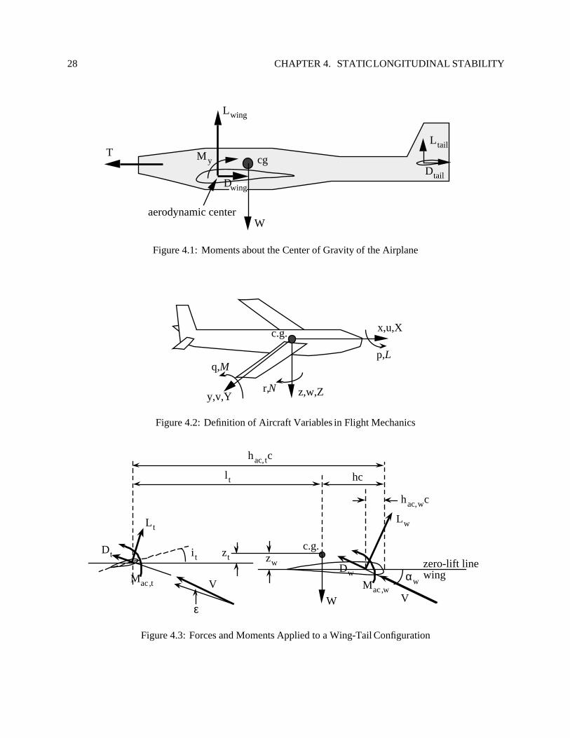
where S is the wing planform area, c is the mean aerodynamic chord and q∞ is the dynamic pressurecorresponding to the freestream velocity V∞. There are numerous places where moments can be generatedin an airplane (Figure 4.1) such as moments contributed by the wing, the fuselage, the engine propulsion,the controls (e.g., elevator, aileron, rudder, canard, etc...) and the vertical and horizontal tail surfaces. Notethat the gravity force does not contribute any moment to the airplane since it is, by definition, applied atthe center of gravity. The aerodynamic center for the wing is defined as the point about which the momentMac (or its moment coefficient CM,ac ) is independent of the angle of attack. This point is convenient for thederivation of the moment equation since it isolates out the part that is independent of the angle of attack.
4.1 Notations and Sign Conventions
Hereweintroducethecommonlyusednotationsfordisplacements,velocities,forcesandmomentsinstability,control and flight mechanics. The origin of the axis system defined by the x , y, z-coordinates is assumedfixed to the center of gravity of the airplane (see Figure 4.2). It will move and rotate with the aircraft. The xdisplacement has a positive forward direction, the y displacement has a positive direction to the right-wingdirectionwhile the z displacementis pointedpositively downward. Therespective componentsofthe aircraftvelocity V in the x, y and z directions are (u, v,w) respectively. The total force F applied to the airplanehas components (X, Y, Z) while the respective moment components are (L , M, N). Note that all the forcesand moments are assumed to apply at the center of gravity.
We will examine a simple airplane configuration in our analysis of longitudinal static stability. The basicairplane consists simply of a wing and tail configuration only. This simple configuration will illustrate wellthe basic fundamentals in stability and control analysis.
4.2 Stick-Fixed Stability
The forces and moments of a wing-tail configuration is shown in Figure 4.3. Without loss of generality, the
27
28 CHAPTER 4. STATICLONGITUDINAL STABILITY
T
Lwing
wing
cg
aerodynamic center
L tail
Dtail
My
D
W
Figure 4.1: Moments about the Center of Gravity of the Airplane
y,v,Y z,w,Z
x,u,X
q,Mp,L
r,N
c.g.
Figure 4.2: Definition of Aircraft Variables in Flight Mechanics
V
zero-lift line wingαwV
ε
it
Lw
Dw
Mac ,wMac ,t
L t
Dtc.g.
zt zw
lt hc
hac,wc
hac,tc
W
Figure 4.3: Forces and Moments Applied to a Wing-Tail Configuration

4.2. STICK-FIXED STABILITY 29
horizontal axis is assumed to coincide with the zero-lift line of the wing. Relative to this reference line, thetail is shown to have a positive incidence angle. Note that in our development, we adopt the same standardconvention for all angle definitions (i.e. according to the right-hand rule). The angle of attack of the wingwith respect to the zero-lift line is defined as αw . At the tail, the angle of attack is reduced by an angle ε dueto the downwash at the wing. The airplane is in equilibrium when sums of all the forces and moments aboutthe center of gravity are zero.
In the longitudinal axis, we have
6Fz = W − (Lwcosαw + Dwsin αw) − [L t cos(αw − ε) + Dt sin (αw − ε)]= 0
(4.2)
and
6My = Mac,w + (Lwcosαw + Dwsin αw)(hc − hac,wc) + (Lwsin αw − Dwcosαw)zw+
Mac,t − [L tcos(αw − ε) + Dt sin (αw − ε)]lt + [L t sin (αw − ε) − Dt cos(αw − ε)]zt
= 0
(4.3)
To simplify our analysis, one can usually assume that the angle of attack αw is small and use the followingapproximations for cosαw
∼= 1 and sin αw∼= αw where αw is in radians. Then equations (4.2) and (4.3)
becomeW = (Lw + Dwαw) + [L t + Dt(αw − ε)] (4.4)
andMac,w + (Lw + Dwαw)(h − hac,w)c + (Lwαw − Dw)zw+
Mac,t − [L t + Dt(αw − ε)]lt + [L t(αw − ε) − Dt ]zt = 0(4.5)
Let’sintroducethefollowingdefinitionsfornon-dimensionalforcesandmomentsatthewingandtailsurfaces,
Lw = qS dC Lw
dααw
= qSa wαw
Mac,w = qScC Mac,w
L t = qt StCL t
= qt StdC Ltdα
αt
= qt StdC Ltdα
(it + αw − ε)
= qt Stat (it + αw − ε)
Mac,t = qt StctCMac,t
(4.6)
Furthermore, we define the following
ηt =qt
q(4.7)
ε = εo + dεdα
αw
= εo + εααw(4.8)
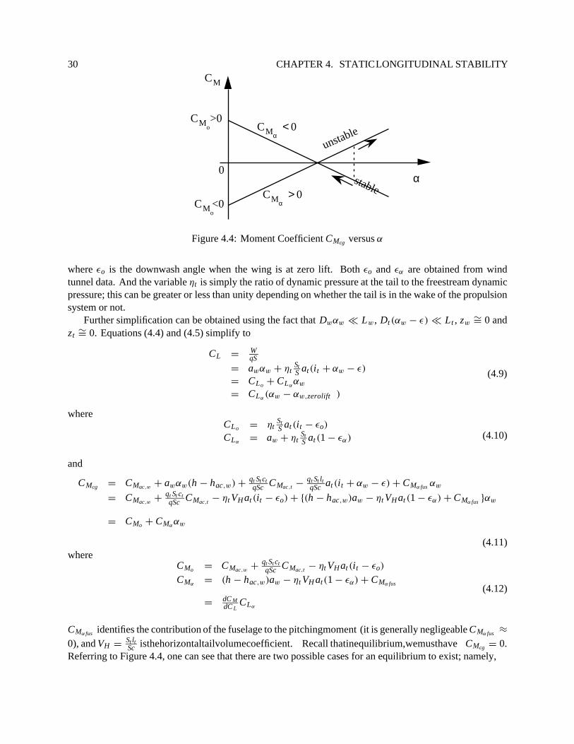
30 CHAPTER 4. STATICLONGITUDINAL STABILITYCM
0α
unstable
stable
CMo>0
CMo<0
CMα< 0
CMα> 0
Figure 4.4: Moment Coefficient CMcg versus α
where εo is the downwash angle when the wing is at zero lift. Both εo and εα are obtained from windtunnel data. And the variable ηt is simply the ratio of dynamic pressure at the tail to the freestream dynamicpressure; this can be greater or less than unity depending on whether the tail is in the wake of the propulsionsystem or not.
Further simplification can be obtained using the fact that Dwαw ¿ Lw , Dt (αw − ε) ¿ L t , zw∼= 0 and
zt∼= 0. Equations (4.4) and (4.5) simplify to
CL = WqS
= awαw + ηtStS at(it + αw − ε)
= CLo + CLααw
= CLα(αw − αw,zerolift )
(4.9)
whereCLo = ηt
StS at (it − εo)
CLα= aw + ηt
StS at (1 − εα) (4.10)
and
CMcg = CMac,w+ awαw(h − hac,w) + qt St ct
qSc CMac,t − qt St ltqSc at (it + αw − ε) + CMα fus αw
= CMac,w+ qt St ct
qSc CMac,t − ηt VH at (it − εo) + {(h − hac,w)aw − ηt VH at (1 − εα) + CMα fus }αw
= CMo + CMααw
(4.11)where
CMo = CMac,w+ qt St ct
qSc CMac,t − ηt VH at (it − εo)
CMα= (h − hac,w)aw − ηt VH at(1 − εα) + CMα fus
= dC MdC L
CLα
(4.12)
CMα fus identifies the contribution of the fuselage to the pitchingmoment (it is generally negligeable CMα fus ≈
0), and VH = St ltSc isthehorizontaltailvolumecoefficient. Recall thatinequilibrium,wemusthave CMcg = 0.
Referring to Figure 4.4, one can see that there are two possible cases for an equilibrium to exist; namely,
4.2. STICK-FIXED STABILITY 31
1. CMo > 0 and CMα< 0: This case corresponds to a statically stable equilibrium point since for any
small change in the angle of attack, a restoring momentis generated to bring it back to the equilibrium.
2. CMo < 0 and CMα> 0: This case corresponds to a statically unstable equilibrium point since the
moment created due to any change in angle of attack will tend to increase it further.
There exists a location of the center of gravity, i.e. when h = hn, where the coefficient CMα= 0. Recall that
VH = St ltSc (Tail volume coefficient) and lt = (hac,t − h)c, then equation (4.12) becomes, with h substituted
by hn,
(hn − hac,w)aw − ηt (hac,t − hn)St
Sat (1 − εα) + CMα fus = 0 (4.13)
or
[aw + ηtSt
Sat (1 − εα)]hn = hac,waw + ηt
St
Sat (1 − εα)hac,t − CMα fus (4.14)
Let’s examine the total lift on the wing-tail configuration, it is given by
L = Lw + L t
= qSa wαw + qt St at(it + αw − ε)
= qSa wαw + qt St at{it − εo + αw(1 − εα)}
(4.15)
or the total lift coefficient CL is
CL = ηtStS at (it − εo) + [aw + ηt
StS at(1 − εα)]αw
= CLo + CLααw
(4.16)
Thus, the combined lift curve slope is
CLα= aw + ηt
St
Sat(1 − εα) (4.17)
From the above definition of CLα, equation (4.14) is simplified to the following
CLαhn = hac,waw + (CLα
− aw)hac,t − CMα fus (4.18)
or the neutral point hn is given by
hn =hac,w + [CLα
aw− 1]hac,t
CLα
aw
−CMα fus
CLα
(4.19)
or
hn = hac,t − aw
CLα(hac,t − hac,w) −
CMα fus
CLα
From the above, it can be easily shown that
CMα= CLα
(h − hn) (4.20)
Note that CLα> 0, thus CMα
< 0 if (h − hn) < 0 or, the center of gravity must be ahead of the neutral point.The other condition CMo > 0, where CMo is defined in equation (4.12), will be satisfied if the tail incidenceangle it is negative. The quantity (hn − h) is called the static margin. It represents the distance (expressed asa fraction of the mean aerodynamic chord) that the center of gravity is ahead of the neutral point. Roughly,a desireable static margin of at least 5% is recommended. For airplane with relaxed static stability, the staticmargin is negative. A stability augmentation system (SAS) is needed to fly these vehicle.

32 CHAPTER 4. STATICLONGITUDINAL STABILITY
Example 1
Given a light airplane with the following design parameters,
• Wing area Sw = 160.0 f t2, Wing span bw = 30 f t ,
• Horizontal tail area St = 24.4 f t2, Tail span bt = 10 f t ,
• hac,t = 2.78
• Wing with 652 − 415 type airfoil, CMac,w= −0.07 , hac,w = 0.27,
• ηt∼= 1 and εα
∼= 0.447.
The lift curve slopes at the wing and tail are obtained from the following empirical equation,
a3D = a2DA
A + [2(A + 4)/(A + 2)](4.21)
where A = b2/S is the aspect ratio of the surface and no sweep. Thus, with a2D = 2π per radians = 0.106per degrees, we have
aw = 0.0731per degreesat = 0.0642per degrees
(4.22)
The total lift curve slope according to equation (4.17) is CLα= 0.0785 per degrees, and the neutral point is
at hn = 0.443. ThenCMα
= 0.0785(h − 0.443) (4.23)
Calculation of CMac , Aerodynamic Center Location and Mean Aerodynamic Chord (mac) fora Finite Wing
Consider a finite wing shown in Figure 4.5. The locus of the section aerodynamic centers defines the sweptback angle 3. The pitching moment about a line through the point A and normal to the chord line is givenby
MA = q∫ b/2
−b/2c2Cmac dy − q
∫ b/2
−b/2cCl y tan 3dy (4.24)
Then if X A is the distance of the aerodynamic center behind the point A, then
Mac = MA + LX A (4.25)
or
CMac = CMA + CLX A
c(4.26)
Differentiating CMac with respect to α and using the definition of an aerodynamic center yields
0 =dC MA
dα+
X A
cCLα
(4.27)
Substituting equation (4.24) into the above equation and using the fact that
dCmac
dα= 0 (4.28)

4.2. STICK-FIXED STABILITY 33
Α
Λ
V
•y
dLdMac
ytanΛ
c t
co
b2
−b2
0
Figure 4.5: Calculation of Wing Aerodynamic Center
we obtain from equation (4.27),
X A =1
CLαS
∫ b/2
−b/2cClα y tan 3dy (4.29)
If we assume that Clα is constant across the wing span, then we have
X A =
[∫ b/20 cydy
S/2
]Clα
CLα
tan 3 (4.30)
or
X A = yClα
CLα
tan 3 (4.31)
where y is the spanwise distance from the centerline out to the centroid of the half-wing area. As a specialcase, for a linearly tapered wing, equation (4.31) becomes
X A =(1 + 2λ)
(1 + λ)
Clα
CLα
b
6tan 3 (4.32)
where λ = ctco
is the wing taper ratio. The mean aerodynamic chord c of a finite wing is defined as the chordlength that, when multiplied by the wing area S, the dynamic pressure q, and an average CMac , gives the totalmoment about the wing’s aerodynamic center. Namely,
Mac = qS cCMac (4.33)
Combining the above equation with equation (4.24), we have
qS cCMac = q∫ b/2
−b/2c2Cmac dy (4.34)
Thus, if the wing is straight and has constant airfoil cross section (i.e. Cmac is constant across the wing span),then we have c = c. However, if c is not constant (e.g in a tapered wing) and we assume that CMac = Cmac
and Cl are constant across the wing span, then the mean aerodynamic chord c is simply,
c =1
S
∫ b/2
−b/2c2dy (4.35)

34 CHAPTER 4. STATICLONGITUDINAL STABILITY
•
Hinge
ce
c
(a) Stabilizer-Elevator Configuration
δe
+
+
+
δe
it
(b) Stabilator Configuration
Hinge
Figure 4.6: Horizontal Tail Configurations
This integral definition of c is used for any planform. As an example, for a linear tapered wing, we have
c =2co
31 + λ + λ2
1 + λ(4.36)
where co is the midspan chord (Figure 4.5).
4.3 Stick-Free Stability
Wehaveseenintheprevioussectionthekeyelementsinstaticstabilityanalysisforastick-fixedconfiguration.It was assumed that the position of the tail or elevator surface has been fixed by the pilot holding onto thecontrol stick, i.e. to holdthe surfaceintrimmedposition the pilotmust exert aconstant force dueto anonzeromoment at the elevator hinge. This may not be desireable for long duration flight. Of course, nowadays forhighperformanceandlarge-sizeairplane, theproblemisalleviatedwith theuseofpowerassistedcontrolsandseldom there are unassisted control linkages between the pilot controls and the respective control surfaces.
Nevertheless, it would still be necessary for small-size airplanes to investigate the issue of stick-freestability. It turns out that the effect of freeing the control surface amounts to a reduction in static stabilityin a certain configuration (e.g. stabilizer-elevator). Let’s examine the two basic configurations of horizontaltail surfaces: stabilizer-elevator and stabilator as shown in Figure 4.6 .
Horizontal Stabilizer-Elevator Configuration
Let’s consider the moment He about the hinge line of the elevator and the corresponding elevator hingemoment coefficient Che defined as,
Che =He
1/2ρV 2Sece(4.37)

4.3. STICK-FREE STABILITY 35
The elevator hinge moment coefficient Che is found to be a function of the tail angle of attack αt and of theelevator deflection δe. As an approximation, one can write
Che =∂Che
∂αtαt +
∂Che
∂δeδe (4.38)
where ∂Che/∂αt and ∂Che/∂δe are assumed constant and determined empirically (i.e. they vary with theconfigurationoftheplanformofthestabilizer-elevator). Withtheconventionthatapositiveelevatordeflectionis down, these derivative coefficients are usually negative thus producing a negative hinge moment for anypositive change in either αt or δe.
Clearly, the free elevator will reach an equilibrium position when its hinge moment is zero for any tailangle of attack αt . Let’s denote this angle as δe free which is determined by setting Che equal to zero,
Che = 0 =∂Che
∂αtαt +
∂Che
∂δeδe free (4.39)
This equation allows us to solve for δe free in terms of the angle of attack at the tail αt . The tail lift coefficientderived from equation (4.6) is then modified to include the effect of a free elevator as follows,
CL t = atαt +∂CL t
∂δeδe (4.40)
However, since for a stick-free case, δe = δe free , equation (4.40) becomes
CL t = atαt −∂CL t
∂δe
∂Che∂αt
∂Che∂δe
αt (4.41)
orCL t = Featαt (4.42)
where
Fe = 1 −1at
∂CL t
∂δe
∂Che∂αt
∂Che∂δe
= 1 − τ
∂Che∂αt
∂Che∂δe
(4.43)
where τ =∂αt∂δe
is the elevator effectiveness (see Figure 5-33 on page 250 of Perkins & Hage) in
∂CL ,t
∂δe=
∂CL ,t
∂αt
∂αt
∂δe= τat (4.44)
and at is the lift-curve slope of the tail. The variable Fe is called the free elevator factor, and it is usually lessthan unity. Stability analysis for the stick-free case proceeds exactly as in the stick-fixed case. The resultsare obtained simply by substituting at in equation (4.17) by Feat . Namely,
CLα free = aw + ηtSt
SFeat (1 − εα) < CLα fixed (4.45)
The lift curve slope for a stick-free case is always less than that of a stick-fixed case. From the above resultfor CLα free , the neutral point hn is given by
hn free =hac,w + [ CLα free
aw− 1]hac,t
CLα free
aw
−
(CMα
CLα
)
fus
(4.46)

36 CHAPTER 4. STATICLONGITUDINAL STABILITY
or
hn free = hac,t −aw
CLα free(hac,t − hac,w) −
(CMα
CLα
)
fus
(4.47)
Notice that since CLα free < CLα fixed , we deduce that the neutral point for a stick-free case is ahead of theneutral point of a stick-fixed case (i.e. hn free < hn fixed ); hence the stick-free case is less statically stable thanthe stick-fixed case for a given center of gravity position.
From the above, it can be easily shown that
CMα free = CLα free (h − hn free ) (4.48)
Example 2
Using results from Example 1 and assuming that Che = −0.31αt − 0.68δe (where αt and δe are in radians)with an elevator control effectiveness ∂CLt
∂δeof 1.616 per radians. Then
Fe = 1 − 1at
∂CLt∂δe
∂Che /∂αt∂Che /∂δe
= 1 − 10.0642per deg
1.616per rad57.3deg/rad
(−0.31)(−0.68)
= 0.80(4.49)
The lift curve slope CLαis given by
CLα free = aw + ηtStS Feat(1 − εα)
= 0.0731per deg + 1 × 24.4160 0.80 × 0.0642per deg(1 − 0.447)
= 0.0774per deg < CLα fixed = 0.0785per deg(4.50)
The neutral point is at
hn free = 2.78 −0.0731per deg
0.0774per deg(2.78 − 0.27) = 0.4094 < hn fixed = 0.443 (4.51)
Then CMα free = 0.0744(h − 0.4094).
Horizontal Stabilator Configuration
With this configuration, the elevator deflection is mechanically linked to the horizontal stabilator deflectionas follows,
δe = keit + δo (4.52)
The deflection δo is used to provide zero stick force at trim. The hinge moment at the horizontal tail is givenby
Cht =∂Cht
∂αtαt +
∂Cht
∂δeδe (4.53)
Recall that the tail angle of attack αt in a wing-tail configuration is given by αt = it +αw − ε (as in equation(4.6)). Thus the floating incidence angle it at the horizontal stabilator is obtained by letting Cht = 0,
Cht = 0 =∂Cht
∂αt(it + αw − ε) +
∂Cht
∂δe(keit + δo) (4.54)

4.3. STICK-FREE STABILITY 37
or
it = Be{∂Cht
∂αt(1 − εα)αw +
∂Cht
∂δeδo} (4.55)
where the constant Be is defined as
Be =−1
∂Cht∂αt
+∂Cht∂δe
ke
(4.56)
With the above tail incidence angle expressed as a function of αw and δo, one can then determine thecorresponding tail lift coefficient as follows,
CL t = atαt +∂CL t
∂δeδe (4.57)
After some simple algebra that proceeds roughly along the following line,
CL t = at(it + αw − ε) +∂CL t
∂δe(keit + δo) (4.58)
CL t = Feat (1 − εα)αw + Geδo (4.59)
where
Fe = 1 + (1 +1
at
∂CL t
∂δeke)Be
∂Cht
∂αt(4.60)
and
Ge = (at +∂CL t
∂δeke)Be
∂Cht
∂αt+
∂CL t
∂δe(4.61)
Note that in this case, the free elevatorfactor Fe can be greater than unity; hence resultingin an improvementon static margin for the stabilator configuration.
Example 3:[Anderson]
For a wing-body combination, the aerodynamic center lies 0.05c ahead of the center of gravity. The momentcoefficient about the aerodynamic center is CMac,wb = −0.016. If the lift coefficient is CLwb = 0.45, what isthe moment coefficient about the center of gravity?
Note that CMcg,wb = CMac,wb + CLwb(h − hac,wb) where h − hac,wb = 0.05, CLwb = 0.45 and CMac,wb =
−0.016. Thus, CMcg,wb = −0.016 + 0.45(0.05) = 0.0065.
Example 4:[Anderson]
A wing-body model is tested in a subsonic wind tunnel. The lift is found to be zero at a geometric angleof attack α = −1.5o. At α = 5o, the lift coefficient is measured as 0.52. Also at α = 1.0o and 7.88o, themoment coefficients about the center of gravity are measured as −0.01 and 0.05, respectively. The centerof gravity is located at hc = 0.35c. Determine the location of the aerodynamic center and the momentcoefficient about the aerodynamic center CMac,wb .
Knowing the lift coefficients at different angles of attack (CLwb = 0 at α = −1.5o and CLwb = 0.52 atα = 5o) one can deduce the lift curve slope (as a linear approximation) awb as follows,
awb =∂CLwb
∂α=
0.52 − 05 − (−1.5)
= 0.08per deg (4.62)
38 CHAPTER 4. STATICLONGITUDINAL STABILITY
Measuring the moment coefficients about the center of gravity at two different angles of attack and at thesame time we know from previous calculation the lift curve slope, one obtains from
CMcg,wb = CMac,wb + awbαwb(h − hac,wb) (4.63)
the following two linear equations in two unknowns CMac,wb and (h − hac,wb),
−0.01 = CMac,wb + 0.08(1 + 1.5)(h − hac,wb)
0.05 = CMac,wb + 0.08(7.88 + 1.5)(h − hac,wb)(4.64)
From equations (4.64), we can solve for CMac,wb and (h − hac,wb) as
CMac,wb = −0.032, (h − hac,wb) = 0.11 (4.65)
Since h = 0.35, then hac,wb = 0.35 − 0.11 = 0.24.
Example 5:[Anderson]
Consider the wing-body model in Example 4 above. The area and chord of the wing are S = 0.1m2 andc = 0.1m, respectively. Now assume that a horizontal tail is added to the model. The distance of the airplanecenter of gravity to the tail’s aerodynamic center is lt = 0.17m, the tail area is St = 0.02m2, the tail-settingangle is it = −2.7o, the tail lift slope is at = 0.1 per degrees, and from experimental measurement εo = 0o
and ∂ε∂α
= εα = 0.35. If α = 7.88o, what is the moment coefficient CMcg for this airplane model? Does thisairplane have longitudinal static stability and balance? Find the neutral point.
From equation (4.11), we have
CMcg = CMac,w+
qt St ct
qScCMac,t − ηt VH at (it − εo) + {(h − hac,w)aw − ηt VH at (1 − εα)}αw (4.66)
We further assume that the tail has a symmetric airfoil shape where CMac,t = 0. From previous example, wehave CMac,wb = −0.032, aw = 0.08, αw = 7.88o + 1.5o = 9.38o and (h − hac,w) = 0.11. Furthermore
ηt = 1 (assumed )
VH = St ltSC = 0.02(0.17)
0.1(0.1)= 0.34
(4.67)
Thus
CMcg = −0.032− 1(0.34)(0.1)(−2.7 − 0)+{0.11(0.08) − 1(0.34)(0.1)(1 − 0.35)}9.38 = −0.065 (4.68)
For longitudinal static stability, we examine CMαas given in equation (4.12),
CMα= (h − hac,w)aw − ηt VH at (1 − εα) (4.69)
orCMα
= 0.11(0.08) − 1(0.34)(0.1)(1 − 0.35)
= −0.0133 < 0(Statically stable)(4.70)
Is the model longitudinally balanced? To find out we need to determine CMo (defined in equation (4.12) andfrom which we derive the equilibrium angle of attack.
CMo = CMac,w+
qt Stct
qScCMac,t − ηt VH at (it − εo) (4.71)
4.4. OTHER INFLUENCES ON THE LONGITUDINAL STABILITY 39
orCMo = −0.032 − 1(0.34)(0.1)(−2.7 − 0) = 0.0598 (4.72)
Thus, the equilibrium angle of attack is obtained by letting CMcg = 0 in equation (4.11), or
CMcg = CMo + CMααequilibrium
H⇒ αequilibrium = −CMo/CMα= −(0.0598)/(−0.0133) = 4.4962o (4.73)
This angle of attack is within reasonable limits; hence the airplane can be balanced and at the same time itis also statically stable.
The neutral point is given by equation (4.19) as
hn =hac,wb + [CLα
awb− 1]hac,t
CLα
awb
(4.74)
whereCLα
= awb + ηtStS at (1 − εα)
= 0.08 + 1(0.02)/(0.1)(0.1)(1 − 0.35) = 0.093hac,t = h + lt/c = 0.35 + 0.17/0.1 = 2.05
(4.75)
Thus,
hn =0.24 + [0.093
0.08 − 1]2.050.0930.08
= 0.493 (4.76)
One can verifies the above result using equation (4.20), namely
h − hn = CMα/CLα
0.35 − 0.493 = (−0.0133)/(0.093)
−0.143 = −0.143(4.77)
In the following we discuss some other effects that enter into our analysis of the longitudinal static stability.
4.4 Other Influences on the Longitudinal Stability
4.4.1 Influence of Wing Flaps
Changes in the wing flaps affect both trim and stability. Themain aerodynamic effects due to flap deflectionsare:
• Lowering the flaps has the same effect on CMo,wb as an increase in wing camber. That is producing anegative increment in 1CMo,wb .
• Theangleof wing-bodyzero-liftischanged tobemorenegative. Sincethe tailincidence it ismeasuredrelative to the wing-body zero lift line, this in effect places a positive increment in the tail incidenceangle it .
• Change in the spanwise lift distribution at the wing leads to an increase in downwash at the tail, i.e.εo and ∂ε
∂αmay increase.

40 CHAPTER 4. STATICLONGITUDINAL STABILITY
T
V
α p
c.gzp
Nplp
Thrust
Normal Propeller Force
Figure 4.7: Forces on a Propeller
4.4.2 Influence of the Propulsive System
The incremental pitching moment about the airplane center of gravity due to the propulsion system (Figure4.7) is
1Mcg = Tz p + Npl p (4.78)
where T is the thrust and Np is the propeller or inlet normal force due to turning of the air. Another influencecomes from the increase in flow velocity induced by the propeller or the jet slipstream upon the tail, wingand aft fuselage.
In terms of moment coefficient,
1CMcg =T
qS
z p
c+
Np
qS
l p
c(4.79)
Since the thrust is directed along the propeller axis and rotates with the airplane, its contribution to themoment about the center of gravity is independent of αw. Then we have
1CMo =T
qS
z p
c(4.80)
and
1CMα= N prop
Sprop l p
Sc
∂CN p
∂α(1 − εα) (4.81)
where the propeller normal force coefficient ∂CNp/∂α and the downwash (or upwash) εα are usually de-termined empirically (Figure 4.8). N prop is the number of propellers and Sprop is the propeller disk area(= π D2/4) and D is the diameterof the propeller. Notethat a propeller mountedaft of the c.g. isstabilizing.This is one of the advantages of the pusher-propeller configuration. Note that n in Figure 4.8 is the propellerangular speed in rps .
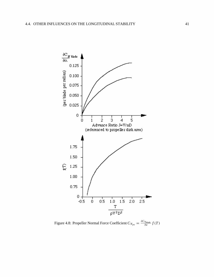
4.4. OTHER INFLUENCES ON THE LONGITUDINAL STABILITY 41
Figure 4.8: Propeller Normal Force Coefficient CNpα=
∂CNblade∂α
f (T )

42 CHAPTER 4. STATICLONGITUDINAL STABILITY
4.4.3 Influence of Fuselage and Nacelles
The pitching moment contributions of the fuselage and nacelles can be approximated as follows (Perkins &Hage p. 229, Equation (5.31)),
CMα fuselage =K f W 2
f L f
Sc(per degrees) (4.82)
where W f is the maximum width of the fuselage or nacelle and L f is the length. The empirical pitchingmoment factor K f is given in Figure 4.9 (NACA TR 711).
Figure 4.9: K f as a Function of the Position of the Wing c/4 Root Chord
4.4.4 Effect of Airplane Flexibility
Flexibility of an airframe under aerodynamic loads is evident in any flight vehicle. The phenomenon thatcouples aerodynamics with structural deformations is studied under the subject of aeroelasticity. There aretwo types of analysis:
• Static behaviour: Herethesteady-statedeformationsof thevehicle structureareinvestigated. Phenom-ena such as aileron reversal, wing divergence and reduction in static longitudinal stability fall underthis category.
• Dynamic behaviour: The major problem of interest is associated with the phenomena of dynamicloading, buffeting and flutter.
Let’s study, for example, the effect of fuselage bending on the tail effectiveness. It can be seen that the angleof attack at the tail is reduced by the fuselage bending according to the following equation,
αt = αwb + it − ε − kL t (4.83)

4.4. OTHER INFLUENCES ON THE LONGITUDINAL STABILITY 43
The tail lift coefficient (with δe = 0) is
CL t = atαt = at (αwb + it − ε − kL t ) (4.84)
orCL t = at (αwb + it − ε − kq t StCL t ) (4.85)
Solving for CL t , we get
CL t =at
1 + kηtqS t at(αwb + it − ε) (4.86)
Thus the tail effectiveness is reduced by a factor 1/[1 + kηtqS tat ] that decreases with increasing speed V inthe dynamic pressure q. This decrease in the tail lift curve slope will cause the neutral point to move forward(i.e. .reduced static stability).
Similarly, it can be shown that the elevator effectiveness is decreased due to fuselage bending since
CL t = at(αwb + it − ε − kL t ) +∂CL t
∂δeδe (4.87)
or solving for CL t , we obtain
CL t =at (αwb + it − ε) +
∂CLt∂δe
δe
1 + kηtqS t at(4.88)
Thus the elevator effectiveness is reduced by the same factor 1/[1 + kηtqS t at ].
4.4.5 Influence of Ground Effect
When the airplane is near the ground to within 20% of the wing span, the wing and tail lift curve slope willincrease by about 10%. At the same time, the downwash is reduced to about half of the normal value, whichrequires a greater elevator deflection to hold the nose up. However, static stability is usually improved bythe ground effect.
The aircraft must have sufficient elevator effectiveness to trim in ground effect with full flaps and fullforward c.g. location, at both power off and full power.

44 CHAPTER 4. STATICLONGITUDINAL STABILITY

Chapter 5
Static Longitudinal Control
We have studied in Section 4 the concept of longitudinal stability of an airplane in trim. It was shown thatstatic stability is primarily governedby the sign of the derivativeof the moment coefficient aboutthe airplanecenter of gravity with respect to the angle of attack, i.e CMα
, being negative. All the above analysis relies onthe fact that one can trim the airplane. The question is what are the controls that allow us to trim the airplane.
5.1 Longitudinal Trim Conditions with Elevator Control
For a steady level flight it is easily seen that the airplane velocity in trim is given by
Vtrim =
√2W
ρSC L trim
(5.1)
Thus if the pilot wants to fly at a lower velocity V < Vtrim , then from equation (5.1), we must have CL trim
(or the angle of attack) increased in order to offset the decrease in dynamic pressure. But increasing theangle of attack away from trim would generate for a statically stable airplane a negative pitching momentthat tends to bring the angle of attack back to the original trim point (Figure 4.4). It would therefore beimpossible to change speed if nothing else is changed about the airplane. It turns out that there are basicallytwo ways to achieve a change in the trim angle of attack. The control concepts are illustrated in Figure 5.1.One possibility is to change the slope of the moment coefficient curve as indicated in Figure 5.1a. Thus, bydecreasing the slope CMα
(i.e more negative), one can achieve a smaller trim angle of attack and hence oneis able to fly at a faster velocity. If we examine equation (4.12), the only way to modify CMα
is to change thelocation of the airplane center of gravity that shows up in both the variables h and VH . This principle is usedextensively in modern hand gliding craft but it is clearly not practical for large fixed wing airplanes. Thealternative is tochange the value of CMo as indicatedin Figure5.1b. It will be shown below that by deflectingthe elevatorin the horizontal tail one can translate the moment coefficient curve upward and downward whilewithout affecting its slope.
Let’sexaminetheeffectofdeflectingtheelevatoronthetailliftcoefficientcurve. Usingasignconventionof positive elevator deflection being downward (or using the right-hand rule for angle), it is clear that adeflected elevator causes the lift curve to shift upward and to the left as shown in Figure 5.2 . The lift curveslope remains unchanged. Now, if we assume that the tail is at a constant angle of attack αt , say αt1 in Figure5.2, then an increase in elevator deflection would lead to an increase in tail lift along the vertical dashed line(Figure 5.2). If we plot the tail lift coefficient CL t as a function of δe when the tail is at a given tail angle of
45
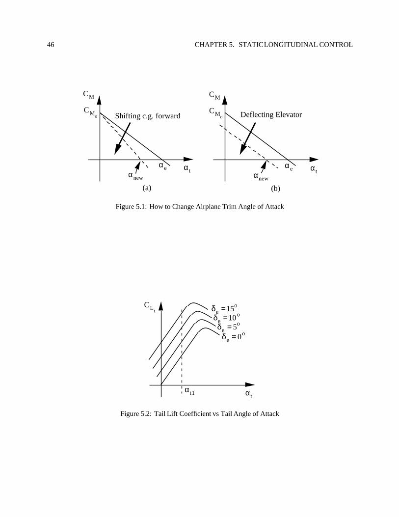
46 CHAPTER 5. STATICLONGITUDINAL CONTROL
CMo
CM
αeαnew
Shifting c.g. forwardCM
o
CM
αeαnew
Deflecting Elevator
αt αt
(a) (b)
Figure 5.1: How to Change Airplane Trim Angle of Attack
αtαt1
δ e = 0o δe = 5o δe = 10o δe = 15oCLt
Figure 5.2: Tail Lift Coefficient vs Tail Angle of Attack
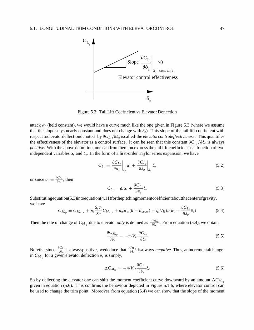
5.1. LONGITUDINAL TRIM CONDITIONS WITH ELEVATORCONTROL 47
CLt
δe
Slope∂CL
t
∂δe αt=cons tan t
>0
Elevator control effectiveness
Figure 5.3: Tail Lift Coefficient vs Elevator Deflection
attack αt (held constant), we would have a curve much like the one given in Figure 5.3 (where we assumethat the slope stays nearly constant and does not change with δe). This slope of the tail lift coefficient withrespect toelevatordeflectiondenoted by ∂CL t /∂δe iscalled the elevatorcontroleffectiveness . This quantifiesthe effectiveness of the elevator as a control surface. It can be seen that this constant ∂CL t /∂δe is alwayspositive. With the above definition, one can from here on express the tail lift coefficient as a function of twoindependent variables αt and δe. In the form of a first-order Taylor series expansion, we have
CL t =∂CL t
∂αt
∣∣∣∣δe
αt +∂CL t
∂δe
∣∣∣∣αt
δe (5.2)
or since at =∂CLt∂αt
, then
CL t = atαt +∂CL t
∂δeδe (5.3)
Substitutingequation(5.3)intoequation(4.11)forthepitchingmomentcoefficientaboutthecenterofgravity,we have
CMcg = CMac,w+ ηt
Stct
ScCMac,t + awαw(h − hac,w) − ηt VH (atαt +
∂CL t
∂δeδe) (5.4)
Then the rate of change of CMcg due to elevator only is defined as∂CMcg
∂δe. From equation (5.4), we obtain
∂CMcg
∂δe= −ηt VH
∂CL t
∂δe(5.5)
Notethatsince ∂CLt∂δe
isalwayspositive, wededuce that∂CMcg
∂δeisalways negative. Thus, anincrementalchange
in CMcg for a given elevator deflection δe is simply,
1CMcg = −ηt VH∂CL t
∂δeδe (5.6)
So by deflecting the elevator one can shift the moment coefficient curve downward by an amount 1CMcg
given in equation (5.6). This confirms the behaviour depicted in Figure 5.1 b, where elevator control canbe used to change the trim point. Moreover, from equation (5.4) we can show that the slope of the moment
48 CHAPTER 5. STATICLONGITUDINAL CONTROL
coefficient curve with respect to angle of attack is not affected (to first-order approximation) by the elevatordeflection. Only the value of CMo is modified by elevator deflection. Namely,
CMcg = (CMo + 1CMcg ) +∂CMcg
∂αwαw
= (CMo − ηt VH∂CLt∂δe
δe) +∂CMcg
∂αwαw
(5.7)
5.1.1 Determination of Elevator Angle for a New Trim Angle of Attack
The problem is to find the elevator deflection δetrim such that the moment coefficient equation is balanced ata new angle of attack αn . We return to equation (5.7) where we substitute αw by αn and using equation (5.6)for 1CMcg
CMcg = 0 = CMo − ηt VH∂CL t
∂δeδetrim +
∂CMcg
∂αw
αn (5.8)
Solving for δetrim , we obtain
δetrim =CMo +
∂CMcg
∂αwαn
ηt VH∂CLt∂δe
(5.9)
Example 6 [Anderson]
Considerafull-sizeairplanewiththeaerodynamic characteristicsdefinedfortheairplanemodelin Examples4 and 5 of Section 4.3. The full-size airplane wing area is S = 19m2 with a weight of W = 2.27 × 10⁴ N ,and an elevator control effectiveness of 0.04. Determine the elevator deflection angle needed to trim theairplane at a velocity of V = 61m/s at sea level.
First, we need to find the airplane angle of attack to fly at V = 61m/s. It is given by
CL =2W
ρV 2S=
2(2.27 × 10⁴)
1.225(61)2(19)= 0.52 (5.10)
From Example 5, we have CLα= 0.093. Then the absolute angle of attack of the airplane is
αn =CL
CLα
=0.52
0.093= 5.59o (5.11)
From equation (5.9), we have
δetrim =CMo +
∂CMcg∂αw
αn
ηt VH∂CLt∂δe
(5.12)
or
δetrim =0.0598 + (−0.0133)(5.59)
1(0.34)0.04= −1.0696o (5.13)
5.1.2 Longitudinal Control Position as a Function of Lift Coefficient
From equation (4.16) we have expressed the total lift coefficient as a function of angle of attack at the wing,constant component of downwash and the tail incidence angle,
CL = CLααw + ηt
St
Sat (it − εo) (5.14)

5.1. LONGITUDINAL TRIM CONDITIONS WITH ELEVATORCONTROL 49
orCL = CLα
αw + CL ti t(it − εo) (5.15)
with
CL ti t= ηt
St
Sat (5.16)
Note that CLαis given in equation (4.17). From equation (5.15), we see that CL is a linear function of angle
of attack αw . Thus for a given CL and tail incidence angle it , one can solve for αw as
αw =CL − CL ti t
(it − εo)
CLα
(5.17)
The other equation of importance is the one for the pitching moment about the airplane center of gravity asgiven in equations (4.11)-(4.12),
CMcg = CMo + CMααw (5.18)
where CMo and CMαare as defined previously in equations (4.12) where CMα
can also be expressed asCMα
= CLα(h − hn). Substituting equation (5.17) and equation (4.12) into equation (5.18) the pitching
moment equation is now a function of the total lift coefficient CL and the tail incidence angle it . Namely,
CMcg = CMac,w+ ηt
St ct
ScCMac,t − ηt VH at(it − εo) + CMα
CL − CL ti t(it − εo)
CLα
(5.19)
For an airplane in trim, one must have CMcg = 0 in equation (5.19). Then one can solve for the tail incidenceangle at a particular CL trim,
it = At + Bt CL (5.20)
where
At = εo +CMac,w+ηt
St ctSc CMac,t
CMα CLti tCLα
+ηt VH at
= εo +CMac,w+ηt
St ctSc CMac,t
ηtStS at [
ltc +h−hn]
(5.21)
andBt =
CMα
CMα CLti t+ηt VH at CLα
= h−hn
ηtStS at [
ltc +h−hn]
(5.22)
Let’s study the sign of the coefficient Bt . Note that for a statically stable airplane, CMα< 0. It can be easily
shown that the denominator term CMαCL ti t
+ ηt VH atCLαis equal to
CMαCL ti t
+ ηt VH at CLα= ηt
St
Sat CLα
(h − hn +lt
c) (5.23)
Thus if lt/c > hn − h, then the coefficient Bt will be negative. Equation (5.22) allows one to determineexperimentally the neutral point. This is done by measuring it as a function of CL for differentc.g. locations.The slopes of the experimentally derived curves are then plotted as a function of center of gravity locations(i.e. h). The neutral point hn is determined by extrapolation to find the value of c.g. that gives a zero slopein ∂it/∂CL (see Figure 5.4). According to equation (5.20) this simply corresponds to having CMα
= 0 orh = hn in equation (4.20).

50 CHAPTER 5. STATICLONGITUDINAL CONTROL
h
•••
•
•
∂it
∂CL
0 hn
Figure 5.4: Determination of Stick-Fixed Neutral Point from Flight Test
5.2 Control Stick Forces
Pilotsusecontrolstickforcesasoneofthemeansofevaluatingtheflyingqualitiesofanairplane. Thus,abilityto control an airplane is quantified in terms of required maximum exerted control forces and its sensitivitywith respect to airspeed. For simple mechanical control systems, the pilot controls are directly linked to therespective control surfaces and the forces he must exert are proportional to the hinge moment (generatedprimarily from aerodynamics) about the pivot point at the surfaces.
Let’s review the key equations governing the analysis of control hinge moments.In the design of airplane control system, the stick (or control wheel) forces must lie within acceptable
limits throughout the operating envelope (V-n diagram) of the airplane. And the gradient of these forceswith respect to airspeed at trim point must produce the proper “feel” to the pilot. In general, the pilot tendsto push forward in the longitudinal control to fly faster and pull on it to slow down. A requirement stated inFAR Part 23 poses a limit on the maximum force of 60 lbs for the stick and 75 lbs for the control wheel.
For analysis, we often assume that the control force P is proportional to the hinge moment H at theelevator. Namely,
P = GH (5.24)
It can be shown that for a system in equilibrium we have Ps + Hδ = 0. Or
δ
H
P
s
Figure 5.5: Longitudinal Control Stick to Stabilator
P = −δ
sH (5.25)
5.2. CONTROL STICK FORCES 51
Thus, G = −δ/s is the gearing ratio which, as derived here, is totally independent of the details of themechanical linkage. Since δ is negative for a positive stick displacement s as shown in Figure 5.5, the hingemoment would be positive for a positive stick force; thus G is positive.
5.2.1 Stick Force for a Stabilator
For a symmetrical airfoil, the pitching moment at the horizontal stabilator is given by
CMt = CMtac (= 0) + CMt αtαt + CMt δe
δe (5.26)
From equation (5.24), we deduce the stick force for the stabilator to be
P = Gqt St ct {CMtαtαt + CMt δe
δe} (5.27)
Note that CMt αtcan be positive or negative depending on whether the aerodynamic center of the stabilator is
ahead or behind the pivot. The coefficient CMt δeis generally negative. The first step is to express αt and δe
in terms of CL . First we recall that the elevator deflection is linked to the horizontal tail incidence as
δe = keit + δo (5.28)
The trim angle of attack αw is determined from the total lift coefficient and the tail angle of incidence it fromthe pitching moment equation in balance. Namely,
CL = awαw + ηtSt
S{at [it − εo + (1 − εα)αw] +
∂CL t
∂δe(keit + δo)} (5.29)
or
CL = CLααw + CL ti t
Feit + ηtSt
S[∂CL t
∂δeδo − atεo] (5.30)
where CLαis given in equation (4.17),
Fe = 1 +1
at
∂CL t
∂δeke (5.31)
and
CL ti t= ηt
St
Sat (5.32)
One can solve for αw in terms of CL , it, δo, εo as follows,
αw =1
CLα
{CL − ηtSt
S
∂CL t
∂δeδo + ηt
St
Satεo − CL ti t
Feit} (5.33)
The other equation we use is the pitching moment about the airplane center of gravity,
CMcg = CMo + CMααw (5.34)
where
CMo = CMac,w+ ηt
St ct
ScCMac,t − ηt VH [at (Feit − εo) +
∂CL t
∂δeδo] (5.35)
andCMα
= (h − hac,w)aw − ηt VH at (1 − εα) = CLα(h − hn) (5.36)
52 CHAPTER 5. STATICLONGITUDINAL CONTROL
Using equations (5.28), (5.33) and the fact that in trim CMcg = 0, we can solve for it in terms of CL, δo, εo.We obtain
it = As + BsCL (5.37)
where
As =1
ηtStS at Fe(
ltc + h − hn)
{CMac,w+ ηt
St ct
ScCMac,t } +
1
Feεo −
1
at Fe
∂CL t
∂δeδo (5.38)
and
Bs =h − hn
ηtStS at Fe(
ltc + h − hn)
(5.39)
Substituting it of equation (5.37) into equation (5.33), we obtain
αw = Aa + BaCL (5.40)
where
Aa = −1
( ltc + h − hn)CLα
{CMac,w+ ηt
St ct
ScCMac,t } (5.41)
and
Ba =
ltc
( ltc + h − hn)CLα
(5.42)
The stick force P given in equation (5.27) becomes
P
GηtqS t ct= [(CMt αt
+ CMt δeke)it + CMt αt
(1 − εα)αw − CMt αtεo + CMtδe
δo] (5.43)
or
P
Gηt qS t ct= [(CMt αt
+ CMt δeke)(As + BsCL) + CMt αt
(1 − εα)(Aa + BaCL )− CMt αtεo + CMt δe
δo] (5.44)
Thus the stick force P is a linear function of CL . By collecting all the terms we have
P
Gηt qS t ct= A + BC L (5.45)
whereA = [(CMt αt
+ CMt δeke)As + CMt αt
(1 − εα)Aa − CMt αtεo + CMt δe
δo] (5.46)
andB = [(CMt αt
+ CMt δeke)Bs + CMt αt
(1 − εα)Ba] (5.47)
Notice that the parameter δo in A can be used to achieve P = 0 at a particular trim velocity Vtrim . That is,
0 = A + BC L trim (5.48)
or A = −BC L trim . We can substitute CL by
CL =W
qS=
W12ρV 2S
(5.49)

5.2. CONTROL STICK FORCES 53
Using equations (5.45) and (5.49), it can be easily shown that
PGηt Stct
= q B(CL − CL trim
)
= q BC L
(1 −
CL trim
CL
)
= (WS )B{1 − V 2
V 2trim
}
(5.50)
Note that Vtrim is given in equation (5.1) and W/S is simply the wing loading.From theabove equation, wecan obtain thegradient of thestick force with respect to speedat V = Vtrim ,
dP
dV
∣∣∣∣V =Vtrim
= −2Gηt StctW
S
B
Vtrim(5.51)
For a given trim speed, a proper stick force gradient as stated in FAR Part 23 must be negative for allconditions of flight. Or B must be positive. Notice that the gradient is large if Vtrim is small. Figure 5.6shows a typical stick force versus speed curve described in equation (5.51). At V = 0, clearly from equation(5.50) we have
P = Gηt StctW
SB (5.52)
P (lb)
60 80 100 120 V(mph)0
10
20
-10
-20
Vtrim = 120
Figure 5.6: Stick Force versus Velocity Curve
5.2.2 Stick Force for a Stabilizer-Elevator Configuration
We proceed as before by first giving the hinge moment associated with the stick force P,
CH = CHo +∂CH
∂αtαt +
∂CH
∂δeδe +
∂CH
∂δtδt (5.53)

54 CHAPTER 5. STATICLONGITUDINAL CONTROL
where in general CHo = 0. Next we examine the total lift coefficient
CL = CLααw + ηt
St
S
∂CL t
∂δeδe − ηt
St
Satεo (5.54)
where we assume that the lift contributed by the trim tab is negligeable. Solve αw in terms of δe and CL ,
αw =1
CLα
{CL − ηtSt
S
∂CL t
∂δeδe + ηt
St
Satεo} (5.55)
Now we consider the pitching moment,
CMcg = CMo + CMααw (5.56)
where
CMo = CMac,w+ ηt
Stct
ScCMac,t + ηt VH [atεo −
∂CL t
∂δeδe] (5.57)
andCMα
= (h − hac,w)aw − ηt VH at (1 − εα) (5.58)
From trim balance with CMcg = 0, we solve for δe
δe = Ae + BeCL (5.59)
where
Ae =1
ηtStS
∂CLt∂δe
( ltc + h − hn)
{CMac,w+ ηt
St ct
ScCMac,t } +
at∂CLt∂δe
εo (5.60)
and
Be =h − hn
ηtStS
∂CLt∂δe
( ltc + h − hn)
(5.61)
Similarly, by substituting equation (5.59) in equation (5.55), we can express αw in terms of CL ,
αw = Aa + BaCL (5.62)
where
Aa = −1
( ltc + h − hn)CLα
{CMac,w+ ηt
St ct
ScCMac,t } (5.63)
and
Ba =
ltc
( ltc + h − hn)CLα
(5.64)
From equations (5.24)) and (5.53), the stick force P becomes
P
Gηt qSece= [
∂CH
∂αt(1 − εα)αw +
∂CH
∂δeδe +
∂CH
∂δtδt ] (5.65)
Thus the stick force P is a linear function of CL . By collecting all the terms we have
P
Gηt qSece= Ae + BeCL (5.66)

5.3. STEADY MANEUVER 55
where
Ae = [∂CH
∂αt(1 − εα)Aa +
∂CH
∂δeAe +
∂CH
∂δtδt] (5.67)
and
Be = [∂CH
∂αt(1 − εα)Ba +
∂CH
∂δeBe] (5.68)
Again the trim tab δt is used to achieve P = 0 at V = Vtrim , then one can simplify the above equation forthe stick force P to the following,
P
Gηt Sece= (
W
S)Be{1 −
V 2
V 2trim
} (5.69)
From the above equation, we obtain the gradient of the stick force with respect to speed at V = Vtrim ,
dP
dV
∣∣∣∣V =Vtrim
= −2Gηt SeceW
S
Be
Vtrim(5.70)
5.3 Steady Maneuver
We now consider the determination of the elevator angle per g in a pull-up maneuver. In the analysis, theconcepts of stick-fixed and stick-free maneuver margins are introduced. For an airplane in a steady pull-upmaneuver, the lift force will exceed the vehicle weight. Namely,
L = W (1 +an
g) (5.71)
where an is the vehicle acceleration. The lift to weight ratio is known as the load factor n or
n = 1 +an
g(5.72)
For a straight level flight, an = 0 and n = 1.We examine the pitching moment of the airplane in this pull-up maneuver from which we derive the
quantity known as elevator angle per g. Again we have
CMcg = CMo + CMααw + 1CM (due to airplane rotation in a steady pull-up maneuver) (5.73)
where
1CM = −qηt Stat1αt lt
qSc= −ηt VH at1αt (5.74)
The incremental angle of attack at the tail due to a constant angular velocity Q is
1αt =lt Q
V(5.75)
or
1αt =2lt
cq (5.76)
with q being the dimensionless pitch rate variable defined as
q =Qc
2V(5.77)

56 CHAPTER 5. STATICLONGITUDINAL CONTROL
5.3.1 Horizontal Stabilizer-Elevator Configuration: Elevator per g
When the airplane is in straight and level flight (unaccelerated), the elevator angle and stick force to trim areδe and P respectively. When in the pull-up maneuver, the elevator is deflected to δe +1δe and the stick forcerequired is P + 1P . The quantities 1δe/(an/g) and 1P/(an/g) are known as the elevator angle per g andthe stick force per g respectively. These are measures of airplane maneuverability; the smaller they are themore maneuverable it is.
Including the effects due to pitch rotation Q in a pull-up maneuver, the pitching moment becomes
CMcg = CMo + CMααw +
∂CM
∂δeδe +
∂CM
∂ QQ (5.78)
Note that Q is not dimensionless and it has the units of rad /s or deg/s. To nondimensionalize Q we usethe variable q defined in equation (5.77). Then equation (5.78) becomes,
CMcg = CMo + CMααw +
∂CM
∂δeδe + CMq q (5.79)
We can derive CMq from 1CM and the expression of 1αt due to Q,
CMq = −ηtat VH2lt
c(5.80)
This term CMq is often referred to as the pitch damping term, since it produces a negative pitching momentdue to a change in pitch rate.
In a steady pull-up there is still no angular acceleration in the pitch axis, thus for equilibrium CMcg = 0as it is in trimmed straight level flight condition. The increment 1CM resulting from a steady maneuver is
1CMcg = 0 = CMα1αw + CMδe
1δe + CMq q (5.81)
where we assume that CMo remains constant in the maneuver. From the above equation, one can solve for1δe as
1δe = −CMα
1αw + CMq q
CMδe
(5.82)
It can be shown that since an = QV we have
q =Qc
2V=
anc
2V 2=
gc
2V 2(an
g) (5.83)
Again the incremental change in angle of attack 1αw is determined from
1CL = CLα1αw +
∂CL
∂δe1δe (5.84)
where 1CL is the incremental lift coefficient due to the pull-up; namely
CL + 1CL
CL=
L
W= 1 +
an
g(5.85)
or1CL =
an
gCL(for 1 g flight) (5.86)

5.3. STEADY MANEUVER 57
Then
1αw =CL
CLα
an
g−
CL δe
CLα
1δe (5.87)
Note that
CLδe=
∂CL
∂δe= ηt
St
S
∂CL t
∂δe(5.88)
or
CL δe= ηt
St
S
∂CL t
∂αt
∂αt
∂δe= ηt
St
S
∂CL t
∂αtτ = ηt
St
Satτ (5.89)
where the coefficient τ can be determined from Figure 5.33 (Perkins & Hage p. 250).Substituting equations (5.83) and (5.87) into equation (5.82) we have
1δe
(an/g)= −
CMαCL + CMq CLα
(gc
2V 2 )
CMδeCLα
− CMαCL δe
(5.90)
Note that W = qSC L = 12ρV 2SC L and W = mg where m is the mass of the airplane. Hence, CL = 2W
ρV 2 S .Also recall that CMδe
= −ηt VH CL t δefrom equation (5.6). Then
1δe
(an/g)= −CLCLα
h − hn + ρSc4m CMq
CMδeCLα
− CMαCLδe
(5.91)
or letting µ = 2mρSc (known as the relative mass parameter), then
1δe
(an/g)= −CLCLα
h − hn + 12µ
CMq
CMδeCLα
− CMαCLδe
(5.92)
Similarly to the neutral point, there is also a particular value of h, known as the stick-fixed maneuver pointdenoted here by hm, forwhich no (i.e. very small) elevator willbe required toproduce a finite (i.e. not small)acceleration. This is determined from equation (5.92) by setting 1δe = 0; namely
hm = hn −1
2µCMq (5.93)
Since CMq < 0, then hm > hn or the stick-fixed maneuver point lies aft of the neutral point. The quantityhm − h is known as the stick-fixed maneuver margin. And we can rewrite equation (5.92) as
1δe
(an/g)=
CLCLα(hm − h)
CMδeCLα
− CMαCL δe
(5.94)
1δe
(an/g)=
CL (hm − h)
CL tδe
[−ηt VH − (h − hn)ηt
StS
] (5.95)
or1δe
(an/g)=
CL (hm − h)
CL tδeηt
StS (hn − hac,t )
< 0 (5.96)

58 CHAPTER 5. STATICLONGITUDINAL CONTROL
5.3.2 Horizontal Stabilator Configuration: Elevator per g
A similar derivation can be performed for the stabilator configuration and we obtain the following results,
1it
(an/g)= −CL CLα
h − hn + 12µ
CMq
CMitCLα
− CMαCL it
(5.97)
where we replace CMδeby CMit
and CLδeby CL it
.
5.3.3 Stabilizer-Elevator Configuration: Stick Force per g
Recall from equation (5.53) that
CH =∂CH
∂αtαt +
∂CH
∂δeδe +
∂CH
∂δtδt (5.98)
assuming that the trim tab has negligeable contribution to the total lift and moment. In a steady pull-up,
αt = it + αw − ε + 2lt
cq (5.99)
or, assuming εo = 0,
αt = it + (1 − εα)αw + 2lt
cq (5.100)
Then the stick force P is given by
P
GηtqS ece= [
∂CH
∂αt[it + (1 − εα)αw +
2lt
cq] +
∂CH
∂δeδe +
∂CH
∂δtδt] (5.101)
Let δt be adjusted to achieve P = 0 at straight level flight (unaccelerated). Then αw = αo + 1αw,δe = δeo + 1δe. It then follows that
1P
Gηt qSece= [
∂CH
∂αt[(1 − εα)1αw +
2lt
cq] +
∂CH
∂δe1δe] (5.102)
Recall that2lt
cq =
glt
V 2(an
g) (5.103)
Thevariables 1αw and 1δe are thoseobtainedin thepreviousanalysis forelevatorper g asgiven inequations(5.87) and (5.96) respectively. Thus, equation (5.102) becomes
1P
GηtqS ece= [
∂CH
∂αt[(1 − εα){
CL
CLα
(an
g) −
CLδe
CLα
1δe} +glt
V 2(an
g)] +
∂CH
∂δe1δe] (5.104)
After some simple manipulations, we obtain
1P
(an/g)= Gηt Sece(
W
S){
∂CH
∂αt[(1 − εα)
CLα
+1
µ
lt
c] +
∂CH∂δe
CLα− ∂CH
∂αt(1 − εα)CLδe
CMδeCLα
− CMαCLδe
(hm − h)} (5.105)

5.3. STEADY MANEUVER 59
Again, there is a position of center of gravity h for which 1P = 0. This is known as the stick-free maneuverpoint denoted by h′
m . It is called the stick-free maneuver point since it corresponds to the fact that the pilotcan let go of his control stick (i.e. stick free). Equation (5.105) can be rewritten as
1P
(an/g)= Gηt Sece(
W
S){
∂CH∂δe
CLα− ∂CH
∂αt(1 − εα)CLδe
CMδeCLα
− CMαCLδe
(h′m − h)} (5.106)
where
h′m = hm +
∂CH
∂αt[(1 − εα)
CLα
+1µ
lt
c]
CMδeCLα
− CMαCLδe
∂CH∂δe
CLα− ∂CH
∂αt(1 − εα)CLδe
(5.107)
One would create a catastrophic situation if we load the airplane such that h = h′m . In this case, the pilot
would inadvertently generate extremely large inertia loads on the airplane by exerting little or no controlforce. Such a situation rarely occurs if the vehicle has an adequate static margin since the stick-fixed andstick-free maneuver points are always aft of the neutral point.
5.3.4 Stabilator Configuration: Stick Force per g
A similar analysis as the one performed for the stabilizer-elevator configuration can also be done for thestabilator configuration. Details are left to the students. (They can be found in the reference book by B. W.McCormick)
Remarks:
• Stick force per g is a linear function of h. For a normal range of c.g. (i.e. h < h′m) locations, the
force gradient is positive. That is the pilot must exert a pull (positive) force on the stick to maneuver apitch up maneuver. The airplane is highly maneuverable if this force gradient is small (i.e. when thec.g. location is near the stick-free maneuver point). In this case, the airplane may even be staticallyunstable.
• Stick force per g is directly proportional to wing loading (W/S).
• It is independent of CL or V apart from Mach and Reynold effects.
60 CHAPTER 5. STATICLONGITUDINAL CONTROL

Chapter 6
Lateral Static Stability and Control
The concept of static stability and control we studied for the longitudinal axis can also be applied to thelateral axis. The key motion variables in the lateral axis correspond to sideslip (with sideslip angle β , or sidevelocity v), roll (with roll rate p) and yaw (with yaw rate r). Primary controls are rudder δr and ailerons δa.
6.1 Yawing and Rolling Moment Equations
The lateral motion of an airplane is described in terms of two tightly coupled motions: yaw about the z-bodyaxis (i.e. directional) and roll about the x-body axis (i.e. lateral).
Using Figure 6.1, let’s first identify the motion variables, the control effectors and their sign conventionsused in the lateral-directional stability analysis.
Note that all along we adhere strictly to the right-hand rule for sign conventions:
• x -body axis pointed forward,
• y-body axis pointed to the right wing,
• z-axis pointed down toward the earth,
• Positive yaw motion (clockwise) (i.e. yaw rate r > 0 with yaw angle ψ),
• Positive roll motion (right wing down) (i.e. roll rate p > 0 with roll angle φ),
• Positive sideslip β = sin −1(v/V ) corresponding to a positive v-component in side velocity.
• Aileron control positive with right aileron down (δar > 0 again consistent with the right-hand rulewhere a positive rotation about the positive y-body axis) and left aileron up (δal > 0). In general, wedefine aileron angle δa to be δa = δar + δal . Notice that this definition of positive aileron will producea negative rolling moment.
• Positive rudder deflection (δr > 0) is to the left (again according to the right-hand rule a positiverotation about the positive z-body axis). With this definition, a positive rudder will generate a negativeyawing moment and a positive side force. This is similar to the definition that a positive elevatordeflection would pitch the airplane down, i.e. producing a negative pitching moment and a positivecontribution to lift.
61

62 CHAPTER 6. LATERAL STATICSTABILITY AND CONTROL
x
yr,N
β
V
v
Tright
δaRδspR
δ r
Fv
p,
Positive down
L
Figure 6.1: Definition of the Lateral Directional Motion of an Airplane
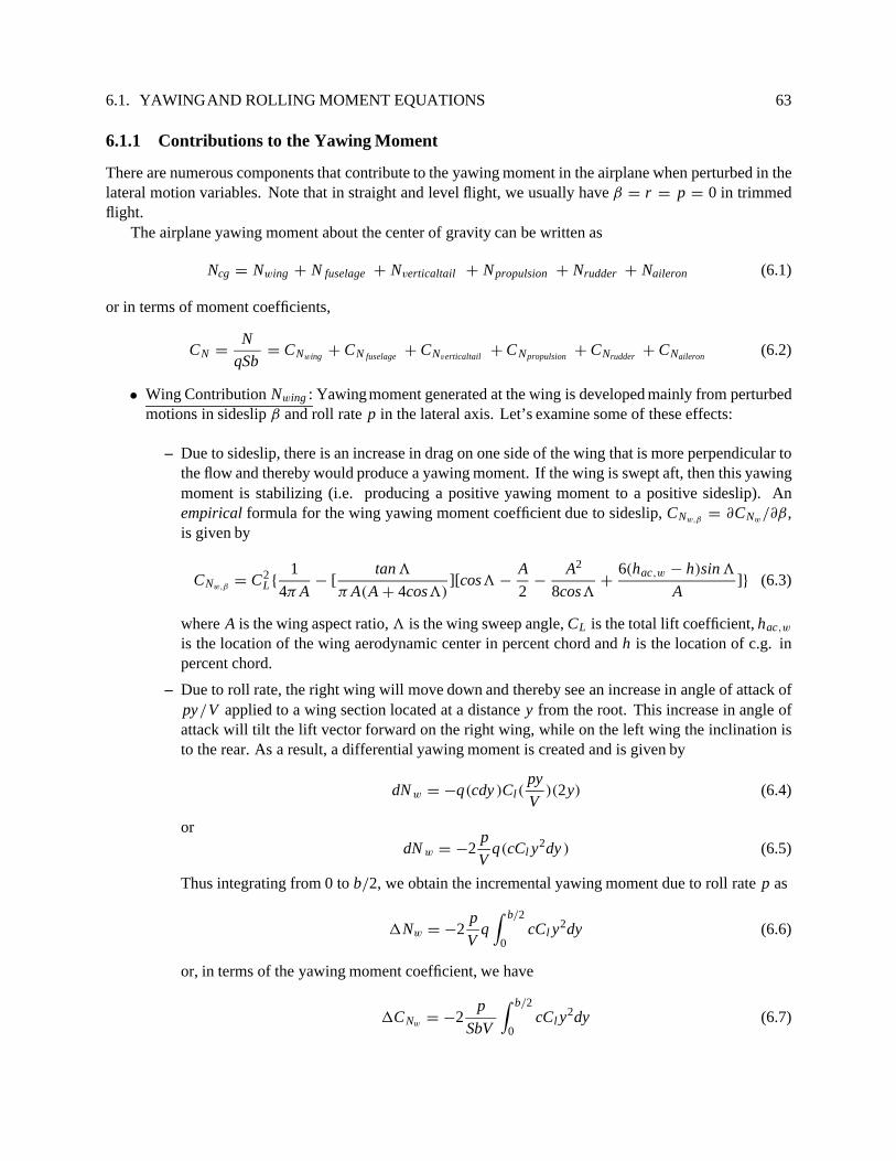
6.1. YAWINGAND ROLLING MOMENT EQUATIONS 63
6.1.1 Contributions to the Yawing Moment
There are numerous components that contribute to the yawing moment in the airplane when perturbed in thelateral motion variables. Note that in straight and level flight, we usually have β = r = p = 0 in trimmedflight.
The airplane yawing moment about the center of gravity can be written as
Ncg = Nwing + N fuselage + Nverticaltail + Npropulsion + Nrudder + Naileron (6.1)
or in terms of moment coefficients,
CN =N
qSb= CNwing + CN fuselage + CNverticaltail + CNpropulsion + CNrudder + CNaileron (6.2)
• Wing Contribution Nwing : Yawing moment generated at the wing is developed mainly from perturbedmotions in sideslip β and roll rate p in the lateral axis. Let’s examine some of these effects:
– Due to sideslip, there is an increase in drag on one side of the wing that is more perpendicular tothe flow and thereby would produce a yawing moment. If the wing is swept aft, then this yawingmoment is stabilizing (i.e. producing a positive yawing moment to a positive sideslip). Anempirical formula for the wing yawing moment coefficient due to sideslip, CNw,β
= ∂CNw/∂β ,
is given by
CNw,β= C2
L {1
4π A− [
tan3
π A(A + 4cos3)][cos3 −
A
2−
A2
8cos3+
6(hac,w − h)sin 3
A]} (6.3)
where A is the wing aspect ratio, 3 is the wing sweep angle, CL is the total lift coefficient, hac,w
is the location of the wing aerodynamic center in percent chord and h is the location of c.g. inpercent chord.
– Due to roll rate, the right wing will move down and thereby see an increase in angle of attack ofpy/V applied to a wing section located at a distance y from the root. This increase in angle ofattack will tilt the lift vector forward on the right wing, while on the left wing the inclination isto the rear. As a result, a differential yawing moment is created and is given by
dNw = −q(cdy )Cl(py
V)(2y) (6.4)
ordN w = −2
p
Vq(cCl y2dy ) (6.5)
Thus integrating from 0 to b/2, we obtain the incremental yawing moment due to roll rate p as
1Nw = −2p
Vq
∫ b/2
0cCl y2dy (6.6)
or, in terms of the yawing moment coefficient, we have
1CNw= −2
p
SbV
∫ b/2
0cCl y
2dy (6.7)

64 CHAPTER 6. LATERAL STATICSTABILITY AND CONTROL
For a linearly tapered wing with taper ratio λ = ct/co and assuming that Cl is constant acrossthe wing span, we can show that
1CNw= −
CL
12
(1 + 3λ
1 + λ
)p (6.8)
or the yawing moment coefficient contributed by the wing due to roll rate is given by
CNw, p = −CL
12
(1 + 3λ
1 + λ
)(6.9)
in terms of the dimensionless roll rate p = pb/2V .
• Fuselage (and Nacelle) Contribution N fuselage : Yawing moment due to sideslip is a function of thefuselage (or nacelle) volume, length and width as follows,
∂CN fuselage
∂β= CN fuselage ,β
= −1.3Volume
Sb(
D f
W f) (per radians) (6.10)
where W f and D f are respectively themaximum widthanddepth ofthe fuselage. Clearly, the fuselageproduces a negative contribution to the lateral stability, i.e., making the vehicle less stable in the yawaxis.
• Vertical Tail Contribution Nverticaltail : The vertical tail plays as significant a role in the lateral motionas the horizontal tail in the longitudinal motion. The effects on the vertical tail due to sideslip, roll rateand yaw rate are described below.
– Due to a sideslip β , the vertical tail produces a side force Fv which in turn will result in yawingmoment about the center of gravity as follows. Note that the side force Fv is given by
Fv = −ηvqSvavβv = −ηvqSvav
∂βv
∂ββ = −ηvqSvav(1 − εβ )β (6.11)
The yawing moment coefficient produced by this side force is
1CNv= CNv,β
β = −FvlvqSb
(6.12)
Using equation (6.11), we deduce
CNv,β= ηv
Sv
Sav
lvb
(1 − εβ) (6.13)
where ηv is the ratiobetween the dynamic pressure at the verticaltail and the freestream dynamicpressure, lv is the distancefrom the aerodynamic center of the vertical tail to the center of gravity,εβ is the sidewash factor.
– Due to roll rate p, points along the vertical tail will see an increase in angle of attack of py/V ,thus we have an incremental yawing moment of,
dN v = qv(cvdy )av
yp
Vlv (6.14)
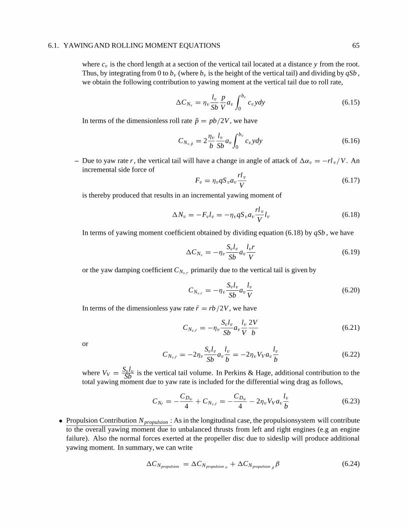
6.1. YAWINGAND ROLLING MOMENT EQUATIONS 65
where cv is the chord length at a section of the vertical tail located at a distance y from the root.Thus, by integrating from 0 to bv (where bv is the height of the vertical tail) and dividing by qSb ,we obtain the following contribution to yawing moment at the vertical tail due to roll rate,
1CNv= ηv
lvSb
p
Vav
∫ bv
0cv ydy (6.15)
In terms of the dimensionless roll rate p = pb/2V , we have
CNv, p = 2ηv
b
lvSb
av
∫ bv
0cv ydy (6.16)
– Due to yaw rate r , the vertical tail will have a change in angle of attack of 1αv = −rl v/V . Anincremental side force of
Fv = ηvqSvav
rlvV
(6.17)
is thereby produced that results in an incremental yawing moment of
1Nv = −Fvlv = −ηvqSvav
rl v
Vlv (6.18)
In terms of yawing moment coefficient obtained by dividing equation (6.18) by qSb , we have
1CNv= −ηv
SvlvSb
av
lvr
V(6.19)
or the yaw damping coefficient CNv,r primarily due to the vertical tail is given by
CNv,r = −ηv
SvlvSb
av
lvV
(6.20)
In terms of the dimensionless yaw rate r = rb/2V , we have
CNv,r = −ηv
SvlvSb
av
lvV
2V
b(6.21)
or
CNv,r = −2ηv
SvlvSb
av
lvb
= −2ηvVV av
lvb
(6.22)
where VV =SvlvSb is the vertical tail volume. In Perkins & Hage, additional contribution to the
total yawing moment due to yaw rate is included for the differential wing drag as follows,
CNr = −CDw
4+ CNv,r = −
CDw
4− 2ηvVV av
lvb
(6.23)
• Propulsion Contribution N propulsion : As in the longitudinal case, the propulsionsystem will contributeto the overall yawing moment due to unbalanced thrusts from left and right engines (e.g an enginefailure). Also the normal forces exerted at the propeller disc due to sideslip will produce additionalyawing moment. In summary, we can write
1CNpropulsion = 1CN propulsion o+ 1CN propulsion β
β (6.24)
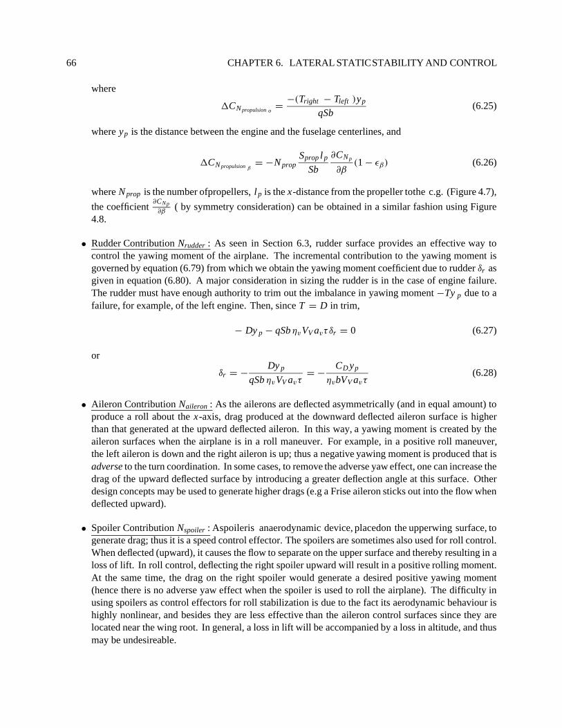
66 CHAPTER 6. LATERAL STATICSTABILITY AND CONTROL
where
1CN propulsion o=
−(Tright − Tleft )yp
qSb(6.25)
where yp is the distance between the engine and the fuselage centerlines, and
1CN propulsion β= −N prop
Sprop l p
Sb
∂CN p
∂β(1 − εβ) (6.26)
where N prop is the number ofpropellers, l p is the x-distance from the propeller tothe c.g. (Figure 4.7),
the coefficient∂CNp
∂β( by symmetry consideration) can be obtained in a similar fashion using Figure
4.8.
• Rudder Contribution Nrudder : As seen in Section 6.3, rudder surface provides an effective way tocontrol the yawing moment of the airplane. The incremental contribution to the yawing moment isgoverned by equation (6.79) from which we obtain the yawing moment coefficient due to rudder δr asgiven in equation (6.80). A major consideration in sizing the rudder is in the case of engine failure.The rudder must have enough authority to trim out the imbalance in yawing moment −Ty p due to afailure, for example, of the left engine. Then, since T = D in trim,
− Dy p − qSbηvVV avτ δr = 0 (6.27)
or
δr = −Dy p
qSb ηvVV avτ= −
CD yp
ηvbVV avτ(6.28)
• Aileron Contribution Naileron : As the ailerons are deflected asymmetrically (and in equal amount) toproduce a roll about the x-axis, drag produced at the downward deflected aileron surface is higherthan that generated at the upward deflected aileron. In this way, a yawing moment is created by theaileron surfaces when the airplane is in a roll maneuver. For example, in a positive roll maneuver,the left aileron is down and the right aileron is up; thus a negative yawing moment is produced that isadverse to the turn coordination. In some cases, to remove the adverse yaw effect, one can increase thedrag of the upward deflected surface by introducing a greater deflection angle at this surface. Otherdesign concepts may be used to generate higher drags (e.g a Frise aileron sticks out into the flow whendeflected upward).
• Spoiler Contribution Nspoiler : Aspoileris anaerodynamic device, placedon the upperwing surface, togenerate drag; thus it is a speed control effector. The spoilers are sometimes also used for roll control.When deflected (upward), it causes the flow to separate on the upper surface and thereby resulting in aloss of lift. In roll control, deflecting the right spoiler upward will result in a positive rolling moment.At the same time, the drag on the right spoiler would generate a desired positive yawing moment(hence there is no adverse yaw effect when the spoiler is used to roll the airplane). The difficulty inusing spoilers as control effectors for roll stabilization is due to the fact its aerodynamic behaviour ishighly nonlinear, and besides they are less effective than the aileron control surfaces since they arelocated near the wing root. In general, a loss in lift will be accompanied by a loss in altitude, and thusmay be undesireable.

6.1. YAWINGAND ROLLING MOMENT EQUATIONS 67
6.1.2 Contributions to the Rolling Moment
Therollingmotionisgenerallyaffectedbythemotionvariablesinyaw r ,sidelip β androll p. Thecomponentsthat contribute mostly to the rolling moment are the wing, the vertical tail, the ailerons (located on the wing)and the rudder.
The airplane rolling moment about the center of gravity can be written as
L = Lwing + L fuselage + Lverticaltail + Laileron + Lrudder (6.29)
In terms of the moment coefficients,
CL =L
qSb= CLwing + CL fuselage + CLverticaltail + CLaileron + CLrudder (6.30)
• Wing Contribution Lwing : The rolling moment produced at the wing is developed primarily fromperturbed motions in sideslip β , roll rate p and yaw rate r .
– Due to sideslip, the rolling moment is primarily obtained from the wing dihedral (depicted bythe dihedral angle 0 > 0 above the horizontal plane). The rate of change of rolling moment withsideslip, CLβ
= ∂CL/∂β, is important to the handling qualities of an airplane. A small negativevalue of CLβ
is desireable. Too much dihedral will make the airplane hard to fly. When theairplane is in a positive sideslip, the right wing will see an increase in angle of attack of
1α = β0V/V = β0 (6.31)
The opposite change in α occurs over the left wing. This results in a differential increment inrolling moment,
dL w = −2q(cdy )awβ0y = −2qawβ0cydy (6.32)
or
CLw= −2awβ0
∫ b/20 cydy
Sb(6.33)
For a linearly tapered wing, we have
CLw= −
aw
6(1 + 2λ
1 + λ)0β (6.34)
or
CLw,β= −
aw
6(1 + 2λ
1 + λ)0 (6.35)
Another effect due to sideslip is derived from a swept-back configured wing. Figure 6.2 shows aswept wing in a positive sideslip. The velocity normal to the right leading edge is V cos(3 − β)
andontheleftwing V cos(3+β). Let Cln bethesection liftcorrespondingtothenormalvelocityV cos(3 − β) (or V cos(3 + β)) and normal chord c cos 3,
Differential lift on the right wing = dL R = q cos2(3 − β)c cos 3Cln ds (6.36)
andDifferential lift on the left wing = dL L = q cos2(3 + β)c cos 3Cln ds (6.37)
The differential rolling moment is simply,

68 CHAPTER 6. LATERAL STATICSTABILITY AND CONTROL
Λ
V V
Vcos(Λ−β)Vcos(Λ+β)
β
y
Γ
Dihedral Angle
βV βVΓ
y
s
Figure 6.2: Effect of Sweepback on Total Lift and Rolling Moment to Sideslip
dL w = (dL L − dL R)y = q[cos2(3 + β) − cos2(3 − β)]c cos 3Cln yds (6.38)
where y = s cos 3 or dy = cos 3ds . Integrating from 0 to b/2 we obtain,
Lw = qC ln [cos2(3 + β) − cos2(3 − β)]∫ b/2
0cydy (6.39)
Note that the incremental lift for a swept wing is
dL =12ρ(Vcos 3)2Cln cdy (6.40)
Hence, integrating over the entire wing span, the total lift for a swept wing is given by
L = 2q cos2 3Cln
∫ b/2
0cdy = qSC ln cos2 3 (6.41)
or the wing CL and the normal section Cln are related by
CL = Cln cos2 3 (6.42)
Then the rolling moment coefficient becomes
CLw=
CL
cos2 3[cos2(3 + β) − cos2(3 − β)]
∫ b/20 cydy
Sb(6.43)

6.1. YAWINGAND ROLLING MOMENT EQUATIONS 69
If we differentiate with respect to β and evaluate the derivative at β = 0, we obtain
CLw,β= −4CL tan 3
∫ b/20 cydy
Sb(6.44)
Again for a linear tapered wing, we have
CLw,β= −
1 + 2λ
3(1 + λ)CL tan 3 (6.45)
Generally, we haveCLw,β
= − f (A, λ)CL tan 3 (6.46)
where f (A, λ) is an empirically derived function of aspect ratio A and taper ratio λ. It shouldbe noted that wing placement on the fuselage combined with the cross-flow over the fuselage insideslip (Figure 6.3) introduces additional factors in the rolling moment due to sideslip, i.e. therolling coefficient CLw,β
,
∗ High wing: 1CLw,β= −0.00016/deg ,
∗ Mid-wing: 1CLw,β= 0,
∗ Low wing: 1CLw,β= +0.00016/deg ,
•
L
More liftLess lift
positive sideslip
High wing
Figure 6.3: Effect of Wing Placement on the Rolling Moment to Sideslip
– Due to roll rate, the resulting effect is related to damping in roll. As the airplane rolls, a sectionon the right wing located at a distance y from the centerline will experience an increase in angleof attack of,
1α =py
V(6.47)
Neglecting induced effects (i.e. tilting of the lift vector), the associated incremental rollingmoment is
dL w = −2q(cdy )aw
py
Vy (6.48)
By integrating from 0 to b/2 and using the nondimensional variable x = y/(b/2), we have
CLw=
Lw
qSb= −
aw A
2(
pb
2V)
∫ 1
0(
c
b)x2dx (6.49)

70 CHAPTER 6. LATERAL STATICSTABILITY AND CONTROL
where A = b2/S is the wing aspect ratio. For a linearly tapered wing, we have
CLw= −
aw
12
1 + 3λ
1 + λp (6.50)
or
CLw, p = −aw
12
1 + 3λ
1 + λ(6.51)
where the dimensionless roll rate is p = pb/2V .
The aileron control can be used to produce constant roll rate in steady-state. It is obtained fromthe following equation,
CLδaδa + CL p p = 0 (6.52)
or
p = −CLδa
CL p
δa (6.53)
– Due to yaw rate, the left wing will see a higher velocity than the right wing which is retractingaway from the forward motion. Assuming that the wing is operating at a constant CL and thesection lift Cl is constant and equals to CL . Then a differential rolling moment is produced fromthe imbalance in dynamic pressure from the two sides; namely
dL w =12ρ[(V + ry )2 − (V − ry )2]CLcdyy (6.54)
dL w = 2ρVrC Lcy2dy (6.55)
Integrating from 0 to b/2, and assuming a straight wing with no taper, we obtain
Lw = 2ρVrC Lc∫ b/2
0y2dy (6.56)
or
Lw =ρcCLrVb 3
12=
1
3qSb rC L (6.57)
Therefore,
CLw=
CL
3r (6.58)
or
CLw,r =dC Lw
dr=
CL
3(6.59)
For a linearly tapered wing, we derive
CLw,r =CL
6
1 + 3λ
1 + λ(6.60)
• Fuselage Contribution L fuselage : In general, there is no contribution of the fuselage to the rollingmoment, i.e. L fuselage = 0.
• Vertical Tail Contribution Lverticaltail :

6.1. YAWINGAND ROLLING MOMENT EQUATIONS 71
– Due to yaw rate, the angle of sideslip is decreased by rl v/V . Thus an increment in side force atthe tail is
Fv = ηvqSvav
rlvV
(6.61)
And the resulting rolling moment is
1Lv = Fvzv = ηvqSvav
rlvV
zv = 2ηvqSvav
rb
2V
lvb
zv = 2ηvqSvav
lvb
zvr (6.62)
where zv is the distance of the aerodynamic center of the vertical tail to the axis of rotation(x-axis) and r = rb
2V is the dimensionless yaw rate variable.Dividing equation (6.62) by qSb , we have
CLv,r = 2ηv
SvlvSb
av
zv
b= 2ηvVV av
zv
b(6.63)
– Due to sideslip, the vertical tail produces a side force Fv as given in equation (6.11). The rollingmoment coefficient produced by this side force is
1CLv= CLv,β
β =Fvzv
qSb= −ηv
qSvav(1 − εβ )βzv
qSb(6.64)
From which we deduce
CLv,β= −ηv
Sv
Sav
zv
b(1 − εβ ) (6.65)
where the variables ηv and εβ are as exactly those defined for equation (6.11).
• Aileron Contribution Laileron : Aileroncontrols areeffectiveinthe generationofrolling momentduetoits location from the axis of rotation (i.e. x -axis). As the right aileron is deflected, there is an increasein sectional lift per unit span produced on the right side. It is given by
dL = qcawdy τδaR (6.66)
where τ istheaileroneffectiveness (SeeFigure9-15ofPerkins&Hage). Thisresultsinanincrementalchange in the rolling moment as follows,
dL = −qcawdyτδaR y (6.67)
Combining with the contribution from the left aileron, we have
dL = −qcawdy τ(δaR − δaL )y (6.68)
Integrating over the spanwise length of the aileron, we obtain
L = −qawτ(δaR − δaL )
∫ y2
y1
cydy (6.69)
In dimensionless form, where we define x = y/(b/2), the above equation (6.69) becomes
CL =Lδa
qSb= −
1
4awτδa A
∫ x2
x1
c
bxdx (6.70)
where A = b2/S is the wing aspect ratio and δa = δaR −δaL . Again for a simple linearly tapered wing,we obtain
CLδa= −awτ
3(x22 − x2
1 ) − 2(1 − λ)(x32 − x3
1)
12(1 + λ)(6.71)

72 CHAPTER 6. LATERAL STATICSTABILITY AND CONTROL
• Rudder Contribution Lrudder : As in equation (6.79) for the yawing moment due to rudder, the rudderwhen deflected will also produce a rolling moment,
1Lδr = zvηvqSvavτδr (6.72)
or, the rolling moment coefficient with respect to δr is given by
CL δr= ηv
Svzv
Sbτav (6.73)
6.2 Directional Stability (Weathercock Stability)
Figure 6.4 shows an airplane at a positive sideslip angle β > 0 or v > 0. The positive yawing moment N isdefined according to the right-hand rule as shown. The non-dimensional yawing moment coefficient is givenby
CN =N
12ρV 2Sb
(6.74)
The change of yawing moment with respect to sideslip β is defined as
CNβ=
∂CN
∂β(6.75)
This quantity has the same significance as the coefficient CMα. However, for stability we see that a positive
yawing moment would be required to bring β back to zero. Therefore, we expect CNβto be positive for
directional static stability.Notethatwhentheairplanehasapositivesideslipthevelocityvectorisnolongerintheplaneofsymmetry.
Thereexistsayawingmomentproducedbythefuselageandbythe sideforceontheverticaltail. Theairplaneis directional stable if CNβ
> 0. Usually the yawing moment due to the fuselage is destabilizing but its effectis small compared to the stabilizing moment contributed by the vertical tail. However, in most situation, thevertical tail is not sized by any consideration of static stability. Instead the minimum tail size is determinedby controllability requirements in the event of an asymmetric engine failure or according to flying qualityrequirements.
If the aerodynamic center of the vertical tail is located a distance of lv behind the center of gravity. Then
N = ηvqSvlvav(1 − εβ)β (6.76)
or
CN =N
qSb= ηv
Sv
S
lvb
av(1 − εβ)β (6.77)
and thus
CNβ= ηt VV av(1 − εβ) (6.78)
where VV = Svlv/Sb is the vertical tail volume, εβ is the sidewash factor (difficult to estimate), av is thelift-curve slope for the vertical tail.

6.2. DIRECTIONAL STABILITY (WEATHERCOCK STABILITY) 73
x
y
Hinge
•
cr
cv
δ r
N
•
∆Lva.c
lv
V β
∆
Figure 6.4: Airplane with a Positive Sideslip

74 CHAPTER 6. LATERAL STATICSTABILITY AND CONTROL
6.3 Directional Control
Effective control of yawing moment is provided by the rudder, a movable surface hinged to the verticalstabilizer. Incremental yawing moment created by the rudder is
1N = −lv1Lv (6.79)
where 1Lv = ηt qSvavτδr and the rate of change of CN with respect to δr is given by
CNδr= −ηvVV avτ (6.80)
where τ is the effective factor which depends on the ratio of cr/cv (For example, see Figure 5-33 of Perkins& Hage).
6.4 Roll Stability
Rollmomentisgeneratedbyasymmetricdeflectionof therightandleftailerons. Whenan airplaneisinitiallyperturbed in roll, and without the use of the aileron controls, there is no physical mechanism to provide arestoring moment. Thus in general CLφ
is always zero and the conceptof static stability does not exist inroll.Or we can also say that the airplane simply possesses neutral static stability in roll. Recall that the rollingmoment coefficient is defined as
CL =L
qSb(6.81)
Dynamic stability in roll motion is governed by the roll damping term in the stability derivative CL p orthe non-dimensional stability derivative CL p . This term is always negative thereby providing positive rolldamping.
6.5 Roll Control
Roll control is provided primarily by the asymmetric deflection of the left and right aileron surfaces. Effec-tiveness oftheaileroncontrol isdeterminedby therollingmomentcoefficient CLδa
derivedinequation(6.71).A small contribution in roll control can be derived from the rudder control as defined by the term CLδr
givenin equation (6.73). In some airplane, additional roll control may be derived from asymmetric deflection ofthe spoilers.

Chapter 7
Review of Rigid Body Dynamics
In general a deformable body of finite dimensions may be regarded as being composed of an infinite numberof particles, thus the system possesses an infinite number of degrees of freedom. This case would apply to adeformable airplane configuration if we take into consideration structural flexibility. However, in this coursewe consider the airplane to be a rigid body with a given mass and moments of inertia. It should be notedthat for a rigid body, the system undergoes no deformation and should possess only 6 degrees of freedom,namely 3 translations and 3 rotations.
To describe completely the motion of a rigid body, it is convenient to use:
• 3 translations of a certain point in the rigid body and
• 3 rotations about that point.
A system of axes attached to the body are called body axes. As shown in Figure 7.1, the motion of the bodycan be described by
1. Translation of the origin O’ of the body axes and
2. Rotation of the axes with respect to the inertial space.
It should be noted that velocity of any point P in the rigid body is given by
VP = VO′ + ω × rP (7.1)
Similarly, acceleration of a point P in the rigid body is given by
aP = aO′ + ω × rP + ω × (ω × rP) (7.2)
Todevelopthe dynamical equationsfor a rigid body, we need firsttodefine itslinear and angularmomentum.Consider Figure 7.1 where OXY Z is the inertial reference axes and O ′xyz corresponds to a set of axesattached to the rigid body. Note that the origin O ′ does not necessarily coincide with the body center of massC . We note the following,
• Mass of the rigid body m is given by
m =
∫
Bodydm (7.3)
75

76 CHAPTER 7. REVIEW OF RIGID BODY DYNAMICS
O'
O
X
Y
Z
(Inertial)
dm
rCrc
p
x
y
z ω
i jk
Figure 7.1: Motion of a Rigid Body
• The mass center C is defined as
rC =1
m
∫
BodyrPdm (7.4)
Note that if the origin O ′ coincides with the center of mass C, we have rC = 0.
• The linear momentum of a rigid body is defined as
p =
∫
BodyVPdm =
∫
Body(VO ′ + ω × rP) dm (7.5)
orp = VO ′
∫
Bodydm + ω ×
∫
BodyrPdm (7.6)
orp = m(VO′ + ω × rC) = mVC (7.7)
where VC is the velocity of the center of mass C . Thus the linear momentum of a rigid body is equalto the product of the total mass m and the velocity of the mass center VC . It should be noted that theabove equation (7.7) applies to any body-axis reference with origin O′. In particular, if O ′ coincideswith the mass center C , we have rC = 0 and VO ′ = VC .
• Now we derive the angular momentum of a rigid body about the origin O ′. By definition,
HO′ =
∫
BodyrP × VPdm (7.8)
orHO ′ =
∫
BodyrP × (VO ′ + ω × rP) dm (7.9)
orHO′ =
∫
BodyrPdm × VO ′ +
∫
BodyrP × (ω × rP) dm (7.10)
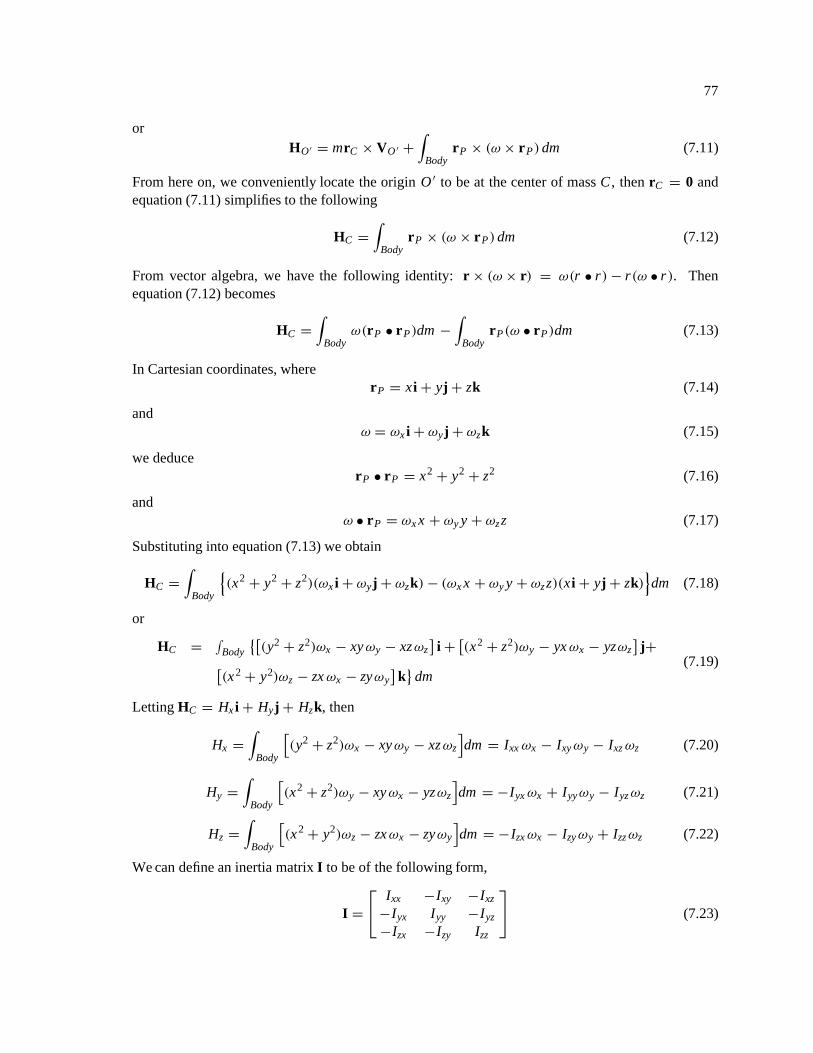
77
orHO′ = mrC × VO ′ +
∫
BodyrP × (ω × rP) dm (7.11)
From here on, we conveniently locate the origin O ′ to be at the center of mass C , then rC = 0 andequation (7.11) simplifies to the following
HC =
∫
BodyrP × (ω × rP) dm (7.12)
From vector algebra, we have the following identity: r × (ω × r) = ω(r • r) − r(ω • r ). Thenequation (7.12) becomes
HC =
∫
Bodyω(rP • rP)dm −
∫
BodyrP(ω • rP)dm (7.13)
In Cartesian coordinates, whererP = xi + yj + zk (7.14)
andω = ωx i + ωyj + ωzk (7.15)
we deducerP • rP = x2 + y2 + z2 (7.16)
andω • rP = ωx x + ωy y + ωzz (7.17)
Substituting into equation (7.13) we obtain
HC =
∫
Body
{(x2 + y2 + z2)(ωx i + ωyj + ωzk) − (ωx x + ωy y + ωzz)(xi + yj + zk)
}dm (7.18)
or
HC =∫
Body
{[(y2 + z2)ωx − xy ωy − xzωz
]i +
[(x2 + z2)ωy − yx ωx − yzωz
]j+
[(x2 + y2)ωz − zx ωx − zyωy
]k}
dm(7.19)
Letting HC = Hx i + Hyj + Hzk, then
Hx =
∫
Body
[(y2 + z2)ωx − xy ωy − xzωz
]dm = Ixx ωx − Ixy ωy − Ixz ωz (7.20)
Hy =
∫
Body
[(x2 + z2)ωy − xy ωx − yzωz
]dm = −Iyx ωx + Iyyωy − Iyz ωz (7.21)
Hz =
∫
Body
[(x2 + y2)ωz − zx ωx − zyωy
]dm = −Izx ωx − Izy ωy + Izz ωz (7.22)
We can define an inertia matrix I to be of the following form,
I =
Ixx −Ixy −Ixz
−Iyx Iyy −Iyz
−Izx −Izy Izz
(7.23)
78 CHAPTER 7. REVIEW OF RIGID BODY DYNAMICS
Notice that the matrix I is a symmetric, positive definite (i.e nonsingular) matrix whose elements haveunits of (ML 2). The angular momentum equation in (7.13) now can be re-written as
HC = Iω (7.24)
where the vector ω is the angular velocity vector of the rigid body with components (ωx , ωy, ωz). Theinertia matrix I is a constant (i.e., not time-varying) matrix since it is defined in the body-axis O ′xyz .Now we can proceed to the development of the equations of motion for a rigid body from Newton’slaws.
7.1 Force Equations
We have from Newton’s laws,dpdt
= F (7.25)
ord
dt(mVC) = F (7.26)
where p = mVC is the linear momentum of the body, m is the total body mass, VC is the velocity of thecenter of mass. Since the rigid body has an angular velocity ω, then equation (7.26) becomes
m (dVC
dt)
∣∣∣∣OXYZ
= m[(dVC
dt)
∣∣∣∣O ′xyz
+ ω × VC ] = F (7.27)
Let the velocity of the center of mass VC = ui + vj + wk and the angular velocity of the rigid body beω = pi + qj + rk where ωx = p, ωy = q and ωz = r . Then the force equations of motion of a rigid bodyairplane are given by
• Along the body O ′x direction:
m(u − rv + qw) = Fx = X force component (7.28)
• Along the body O ′y direction:
m(v − pw + ru ) = Fy = Y force component (7.29)
• Along the body O ′z direction:
m(w − qu + pv) = Fz = Z force component (7.30)
The force components X, Y and Z on the right-hand side of the above equations are due to gravitional force,aerodynamic forces and propulsion forces. We will examine these in the next section. Let’s now proceed tothe equations of motion for the rotational degrees of freedom.

7.2. MOMENT EQUATIONS 79
7.2 Moment Equations
With Newton’s laws applying to the angular momentum, we have
(dHC
dt)
∣∣∣∣OXYZ
= (dHC
dt)
∣∣∣∣O ′xyz
+ ω × HC = M (7.31)
Using equation (7.24), equation (7.31) becomes
Iω + ω × Iω = M (7.32)
Using the above definitions for ω and the inertia matrix I, equation (7.32) can be written in the followingform,
• About the body O ′x direction:
Ixx p − (Iyy − Izz )qr − Iyz (q2 − r2) − Izx (r + pq) − Ixy (q − rp ) = Mx = L (7.33)
• About the body O ′y direction:
Iyy q − (Izz − Ixx )rp − Izx (r 2 − p2) − Ixy ( p + qr ) − Iyz (r − pq) = My = M (7.34)
• About the body O ′z direction:
Izz r − (Ixx − Iyy )pq − Ixy (p2 − q2) − Iyz (q + rp ) − Izx ( p − qr ) = Mz = N (7.35)
The moment components L , M and N on the right-hand side of the above equations are due to aerodynamicforces and propulsion forces. We will examine these in the next section. Note that there is no contributionfrom the gravitational force since these moments are taken about the center of gravity.
7.3 Euler’s Angles
The angular velocity components ωx (or p), ωy (or q) and ωz (or r) about the body axes x , y and z cannotbe integrated to obtain the corresponding angular displacements about these axes. In other words, theorientation of the rigid body in space is not known until we describe the three rotational degrees of freedomin terms of a set of independent coordinates. Of course, such a set is not necessarily unique. One usefulset of angular displacements called Euler’s angles obtained through successive rotations about three (notnecessarily orthogonal) axes as follows.
Formostairplanedynamics,westartwithasetofinertialaxes OXY Z andperformthefollowingrotationsin a particular order (Figure 7.2),
1. Rotation about the Z-axis (i.e yaw) through an angle ψ ⇒ (x1, y1, z1),
2. Rotation about the y1-axis (i.e pitch) through an angle θ ⇒ (x2, y2, z2),
3. Rotation about the x2-axis (i.e roll) through an angle φ ⇒ (x3, y3, z3).
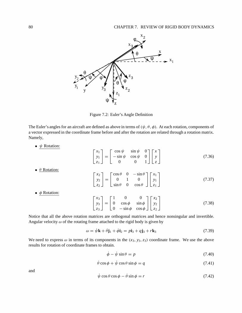
80 CHAPTER 7. REVIEW OF RIGID BODY DYNAMICS
y
z
z1
y1
x
ψ
ψθ
θ
x2
z2
x3
z3φ
y3
φy2
ψ
θ
φ
x1
Figure 7.2: Euler’s Angle Definition
The Euler’s angles for an aircraft are defined as above in terms of (ψ, θ, φ). At each rotation, components ofa vector expressed in the coordinate frame before and after the rotation are related through a rotation matrix.Namely,
• ψ Rotation:
x1
y1
z1
=
cos ψ sin ψ 0− sin ψ cos ψ 0
0 0 1
xyz
(7.36)
• θ Rotation:
x2
y2
z2
=
cos θ 0 − sin θ
0 1 0sin θ 0 cos θ
x1
y1
z1
(7.37)
• φ Rotation:
x3
y3
z3
=
1 0 00 cos φ sin φ
0 − sin φ cos φ
x2
y2
z2
(7.38)
Notice that all the above rotation matrices are orthogonal matrices and hence nonsingular and invertible.Angular velocity ω of the rotating frame attached to the rigid body is given by
ω = ψk + θj1 + φi2 = pi3 + qj3 + rk3 (7.39)
We need to express ω in terms of its components in the (x3, y3, z3) coordinate frame. We use the aboveresults for rotation of coordinate frames to obtain.
φ − ψ sin θ = p (7.40)
θ cos φ + ψ cos θ sin φ = q (7.41)
andψ cos θ cos φ − θ sin φ = r (7.42)
7.3. EULER’S ANGLES 81
Equations (7.40)-(7.42) are solved (i.e integrated) to determine the orientation of the vehicle (φ, θ, ψ) fromthe body angular rates (p, q, r) derived from equations (7.33)-(7.35) when we know the externally appliedmoment components (L , M, N)
We can use the above transformations given in equations (7.36)-(7.38) to express the gravitational forceinto the body components as follows.
Fgravity = mgk = Fx,gravity i3 + Fy,gra vity j3 + Fz,gravity k3 (7.43)
The “flat-earth” model is represented by having the gravitational force always pointed along the vector k.Solving for the components of the gravitational force along the vehicle body axes, we obtain
Fx,gravity = −mg sin θ (7.44)
Fy,gravity = mg cos θ sin φ (7.45)
andFz,gravity = mg cos θ cos φ (7.46)
These components constitute respectively parts of the force components in the right-hand side of equations(7.28)-(7.30). In general, the three successive rotations in equations (7.36)-(7.38) yield the relationshipbetween the coordinates in the two reference frames following the Euler’s angle definition,
x3
y3
z3
=
cos θ cos ψ cos θ sin ψ − sin θ
sin φ sin θ cosψ − cos φ sin ψ sin φ sin θ sin ψ + cos φ cos ψ sin φ cos θ
cos φsin θ cos ψ + sin φ sin ψ cos φ sin θ sin ψ − sin φ cos ψ cos φ cos θ
xyz
(7.47)
Similarly, one can express the coordinates (x, y, z) in terms of the coordinates (x3, y3, z3) by reversing theabove sequence of rotations. Namely,
• −φ Rotation:
x2
y2
z2
=
1 0 00 cos φ − sin φ
0 sin φ cos φ
x3
y3
z3
(7.48)
• −θ Rotation:
x1
y1
z1
=
cos θ 0 sin θ
0 1 0− sin θ 0 cos θ
x2
y2
z2
(7.49)
• −ψ Rotation:
xyz
=
cos ψ − sin ψ 0sin ψ cos ψ 0
0 0 1
x1
y2
z3
(7.50)
This yields the following complete transformation,
xyz
=
cos ψ cos θ − sin ψ cos φ + cos ψ sin θsin φ sin ψ sin φ + cos ψ sin θcosφsin ψ cos θ cos ψ cos φ + sin ψ sin θ sin φ − cos ψ sin φ + sin ψ sin θ cos φ
− sin θ cos θ sin φ cos θ cos φ
x3
y3
z3
(7.51)

82 CHAPTER 7. REVIEW OF RIGID BODY DYNAMICS
The above transformation can be used to determine the aircraft position in terms of its linear velocity V withcomponents (u, v, w) in the body-fixed axis. First we make the observation
«r = xi + yj + zk = ui3 + vj3 + wk3 (7.52)
or
xyz
=
cos ψ cos θ − sin ψ cos φ + cos ψ sin θsin φ sin ψ sin φ + cos ψ sin θcosφsin ψ cos θ cos ψ cos φ + sin ψ sin θ sin φ − cos ψ sin φ + sin ψ sin θ cos φ
− sin θ cos θ sin φ cos θ cos φ
uv
w
(7.53)Expanding the above expression, we have
x = u cos ψ cos θ + v(− sin ψ cos φ + cos ψ sin θsin φ) + w(sin ψ sin φ + cos ψ sin θcosφ) (7.54)
y = u sin ψ cos θ + v(cos ψ cos φ + sin ψ sin θ sin φ) + w(− cos ψ sin φ + sin ψ sin θ cos φ) (7.55)
andz = −u sin θ + v cos θ sin φ + w cos θ cos φ (7.56)
Let’s summarize here the equations governing the motion of a rigid body aircraft.
• Linear momentum equations:
– Along the body O ′x direction:
u = rv − qw − g sin θ +1m
(Xaero + X propulsion ) (7.57)
– Along the body O ′y direction:
v = pw − ru + g sin φ cos θ +1m
(Yaero + Ypropulsion ) (7.58)
– Along the body O ′z direction:
w = qu − pv + g cos θ cos φ +1
m(Zaero + Z propulsion ) (7.59)
• Angular momentum equations:ω = I−1(−ω × Iω + M) (7.60)
• Equations for the vehicle attitude rates:
φ
θ
ψ
=
1 0 − sin θ
0 cos φ cos θ sin φ
0 − sin φ cos θ cos φ
−1
pqr
(7.61)
or
θ = q cos φ − r sin φ
ψ = q sin φsecθ + r cos φsecθ
φ = p + q sin φtan θ + r cos φtan θ
(7.62)
7.3. EULER’S ANGLES 83
• Equations for Earth-relative velocities:
– x -distance:
x = u cos ψ cos θ + v(− sin ψ cos φ + cos ψ sin θsin φ) + w(sin ψ sin φ + cos ψ sin θcosφ)
(7.63)
– y-distance:
y = u sin ψ cos θ + v(cos ψ cos φ + sin ψ sin θ sin φ) + w(− cos ψ sin φ + sin ψ sin θ cos φ)
(7.64)
– Vertical altitude h = −z:
h = u sin θ − v cos θ sin φ − w cos θ cos φ (7.65)
In the above equations, the external forces F and moments M (about the center of gravity) on the right-handside remain tobe determined. They are derived from basic aerodynamic and propulsionforces and moments.In the above derivation, we made the following assumptions:
• Rigid airframe
• Flat Earth (i.e gravity is always pointing in the vertical k direction)
• Axes fixed to the body with origin at the center of gravity
• Earth-fixed reference is treated as inertial reference

84 CHAPTER 7. REVIEW OF RIGID BODY DYNAMICS

Chapter 8
Linearized Equations of Motion
8.1 Linearized Linear Acceleration Equations
Major contributions to the forces and moments in a flight vehicle are coming from the aerodynamics ofwings, body and tail surfaces. It would be difficult to express these in terms of the vehicle motion variablesu, v and w. However it is much easier to express them in terms of the vehicle velocity V , angle of attackα and angle of sideslip β . As shown in Figure 8.1, we can express the linear velocities (u, v, w) directly interms of V, α, β through the following relations:
u = V cos β cos α
v = V sin β
w = V cos β sin α
(8.1)
where V is the aircraft velocity, α is the aircraft angle of attack and β the aircraft sideslip.
αβ
V
Vcosβ
O' x
y
z
Vcosβcosα
VcosβsinαVsinβ
Figure 8.1: Definition of Angle of Attack α and Sideslip β
We can rewrite the linear equations of motion given in equations (7.28)-(7.30) as follows,
u = rv − qw − g sin θ + X/mv = pw − ru + g sin φ cos θ + Y/mw = qu − pv + g cos θ cos φ + Z/m
(8.2)
85
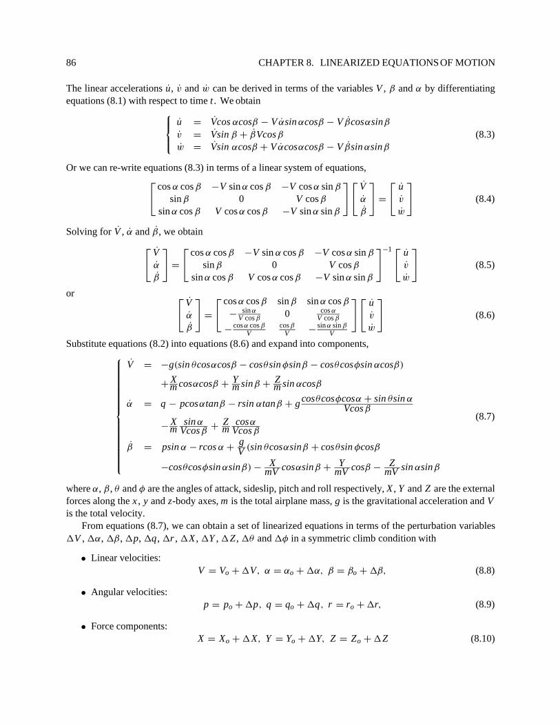
86 CHAPTER 8. LINEARIZED EQUATIONS OF MOTION
The linear accelerations u, v and w can be derived in terms of the variables V , β and α by differentiatingequations (8.1) with respect to time t . We obtain
u = Vcos αcosβ − V αsin αcosβ − V βcosαsinβ
v = Vsin β + βVcosβ
w = Vsin αcosβ + V αcosαcosβ − V βsin αsinβ
(8.3)
Or we can re-write equations (8.3) in terms of a linear system of equations,
cos α cos β −V sin α cos β −V cos α sin β
sin β 0 V cos β
sin α cos β V cos α cos β −V sin α sin β
Vα
β
=
uv
w
(8.4)
Solving for V , α and β , we obtain
Vα
β
=
cos α cos β −V sin α cos β −V cos α sin β
sin β 0 V cos β
sin α cos β V cos α cos β −V sin α sin β
−1
uv
w
(8.5)
or
Vα
β
=
cos α cos β sin β sin α cos β
− sinαV cos β
0 cos αV cos β
− cosα cos βV
cosβV − sinα sin β
V
uv
w
(8.6)
Substitute equations (8.2) into equations (8.6) and expand into components,
V = −g(sin θcosαcosβ − cosθsin φsinβ − cosθcosφsin αcosβ)
+ Xm cosαcosβ + Y
m sinβ + Zm sin αcosβ
α = q − pcosαtanβ − rsin αtanβ + g cosθcosφcosα + sin θsin αVcosβ
− Xm
sin αVcosβ
+ Zm
cosαVcos β
β = psin α − rcos α +gV (sin θcosαsinβ + cosθsin φcosβ
−cosθcosφsin αsinβ) − XmV cosαsinβ + Y
mV cosβ − ZmV sin αsinβ
(8.7)
where α, β , θ and φ are the angles of attack, sideslip, pitch and roll respectively, X , Y and Z are the externalforces along the x , y and z-body axes, m is the total airplane mass, g is the gravitational acceleration and Vis the total velocity.
From equations (8.7), we can obtain a set of linearized equations in terms of the perturbation variables1V , 1α, 1β , 1p, 1q, 1r , 1X , 1Y , 1Z , 1θ and 1φ in a symmetric climb condition with
• Linear velocities:V = Vo + 1V, α = αo + 1α, β = βo + 1β, (8.8)
• Angular velocities:p = po + 1p, q = qo + 1q, r = ro + 1r, (8.9)
• Force components:X = Xo + 1X, Y = Yo + 1Y, Z = Zo + 1Z (8.10)
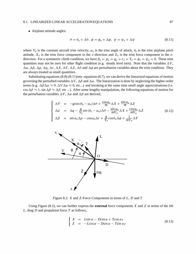
8.1. LINEARIZED LINEAR ACCELERATIONEQUATIONS 87
• Airplane attitude angles:
θ = θo + 1θ, φ = φo + 1φ, ψ = ψo + 1ψ (8.11)
where Vo is the constant aircraft trim velocity, αo is the trim angle of attack, θo is the trim airplane pitchattitude, Xo is the trim force component in the x-direction and Zo is the trim force component in the z-direction. For a symmetric climb condition, we have βo = po = qo = ro = Yo = φo = ψo = 0. These trimquantities may not be zero for other flight condition (e.g. steady level turn). Note that the variables 1V ,1α, 1β , 1p, 1q, 1r , 1X , 1Y , 1Z , 1θ and 1φ are perturbation variables about the trim condition. Theyare always treated as small quantities.
Substituting equations (8.8)-(8.11)into equations (8.7), we can derive the linearized equations of motiongoverning the perturbed variables 1V , 1β and 1α. The linearization is done by neglecting the higher-orderterms (e.g. 1β1α ≈ 0, 1V 1α ≈ 0, etc...) and invoking at the same time small angle approximations (i.e.cos 1β ≈ 1, sin 1β ≈ 1β, etc ...). After some lengthy manipulation, the following equations of motion forthe perturbation variables 1V , 1α and 1β are derived,
1V = −gcos(θo − αo)1θ +cosαo
m 1X +sin αo
m 1Z
1α = 1q −gVo
sin (θo − αo)1θ −sin αomVo
1X +cosαomVo
1Z
1β = sin αo1p − cosαo1r +gVo
cosθo1φ + 1mVo
1Y
(8.12)
x
O
L
T
D
V
z
mg
αθ
αT
X
Ζ
Figure 8.2: X and Z-Force Components in terms of L , D and T
Using Figure (8.2), we can further express the external force components X and Z in terms of the liftL , drag D and propulsion force T as follows,
{X = Lsin α − Dcosα + Tcos αT
Z = −Lcos α − Dsin α − Tsin αT(8.13)
88 CHAPTER 8. LINEARIZED EQUATIONS OF MOTION
Again we can define L = Lo + 1L , D = Do + 1D and T = To + 1T . The trim conditions are nowdetermined from force balance with the gravity force mg. Namely,
{Xo = Losin αo − Docosαo + TocosαT = mgsin θo
Zo = −Locosαo − Dosin αo − Tosin αT = −mgcos θo(8.14)
and {1X = (Locosαo + Dosin αo)1α + sin αo1L − cosαo1D + cosαT 1T1Z = (Losin αo − Docosαo)1α − cosαo1L − sin αo1D − sin αT 1T
(8.15)
Substituting equations (8.15) into equations (8.12), we express the linearized equations in terms of 1L , 1D,1T and 1Y ,
1V = −gcos(θo − αo)1θ −Tosin (θo + αT )
m 1α − 1m 1D +
cos(αo + αT )m 1T
1α = 1q −gVo
sin (θo − αo)(1θ − 1α) −Tocos(θo + αo)
mVo1α
−sin (αo + αT )
mVo1T − 1
mVo1L
1β = sin αo1p − cosαo1r +gVo
cosθo1φ + 1mVo
1Y
(8.16)
We also note that {Do + mgsin (θo − αo) − Tocos(αo + αT ) = 0Lo − mgcos (θo − αo) + Tosin (αo + αT ) = 0
(8.17)
Equations (8.16) then reduce to
1V = −gcos (θo − αo)1θ −Lom 1α − 1
m 1D +cos(αo + αT )
m 1T
1α = 1q −gVo
sin (θo − αo)1θ − DomVo
1α − 1mVo
1L −sin (αo + αT )
mVo1T
1β = sin αo1p − cosαo1r +gVo
cosθo1φ + 1mVo
1Y
(8.18)
The above equations are the linearized equations of the linear acceleration equations. To complete theseequations, one needs to express in details the terms involved in 1L , 1D, 1T and 1Y as a function of thevehicle motion variables and their perturbations. In the next section, we proceed to formulate the linearizedequations of motion corresponding to the angular velocity components p, q and r .
8.2 Linearized Angular Acceleration Equations
According to equations (7.33)-(7.35) and examining the condition related to a steady level climb condition,with the angular velocities defined as
p = po + 1pq = qo + 1qr = ro + 1r
(8.19)
and the moments as
L = Lo + 1LM = Mo + 1MN = No + 1N
(8.20)

8.2. LINEARIZED ANGULAR ACCELERATIONEQUATIONS 89
Notice that for a steady level climb condition, po = qo = ro = 0 and Lo = Mo = No = 0. Substitutingequations (8.19) into equations (7.33)-(7.35) and retaining only the first-order terms in 1p, 1q and 1r , weobtain
• About the O ′y direction:
Iyy1q − (Izz − Ixx )1r1p − Izx (1r2 − 1p2) − Ixy (1 p − 1q1r) − Iyz (1r − 1p1q) = 1M
or, after neglecting all the high-order terms,
Iyy1q − Ixy 1 p − Iyz1r = 1M (8.21)
Assuming further that the airplane has a symmetry about the O ′xz plane then we have Ixy = Iyz = 0.Equation (8.21) now simplifies greatly to
Iyy 1q = 1M (Pitching equation) (8.22)
• About the O ′x direction:
Ixx 1 p − (Iyy − Izz )1q1r − Iyz (1q2 − 1r2) − Ixz (1r + 1q1p) − Ixy (1q − 1r1p) = 1L
or, after neglecting all the high-order terms,
Ixx 1 p − Ixz 1r = 1L (Rolling equation) (8.23)
Note that in general Ixz 6= 0.
• About the O ′z direction:
Izz1r − (Ixx − Iyy )1p1q − Ixy (1p2 − 1q2) − Iyz (1q + 1r1p) − Izx (1 p − 1q1r) = 1N
or, after neglecting all the high-order terms,
Izz 1r − Izx 1 p = 1N (Yawing equation) (8.24)
In summary, the equations describing the angular accelerations of the vehicle are given by
Iyy 0 00 Ixx −Ixz
0 −Izx Izz
1q1 p1r
=
1M1L1N
(8.25)
To complete these equations, one needs to express in details the terms involved in 1M , 1L and 1N as afunction of the vehicle motion variables and their perturbations. The vehicle attitudes are described usingthe Euler’s angles. In the next section, equations that describe the vehicle attitudes for small perturbationangles are developed.

90 CHAPTER 8. LINEARIZED EQUATIONS OF MOTION
8.3 Linearized Euler’s Angle Equations
From equations (7.40)-(7.42), and assuming the trim conditions as defined in equations (8.8)-(8.11),we have
• For the pitch angle θ :1θcos1φ + 1ψcos(θo + 1θ)sin 1φ = 1q
Since cos1φ ≈ 1 and 1ψsin 1φ ≈ 0, then
1θ = 1q (Pitch angle equation) (8.26)
• For the yaw (heading) angle ψ:
1ψcos(θo + 1θ)cos1φ − 1θsin 1φ = 1r
or1ψ(cosθo − sin θo1θ) = 1r
Further simplification yields
1ψ =1
cosθo1r (Yaw angle equation) (8.27)
• For the bank angle φ:1φ − 1ψsin (θo + 1θ) = 1p
or1φ − 1ψ(sin θo + cosθo1θ) = 1p
Again, ignoring the high-order terms,
1φ − sin θo1ψ = 1p (Bank angle equation) (8.28)
Using equation (8.27), the above equation simplifies to
1φ = 1p + tan θo1r (8.29)
8.4 Forces and Moments in terms of their Coefficient Derivatives
In this section, the lift, drag and propulsion forces are expressed in terms of the motion variables and theirperturbations; similarly, for moments about the vehicle axes. Results are represented in terms of the vehiclestability derivatives.
Let’s define the following dimensionless motion related variables,
p = pb/(2Vo)
q = qc/(2Vo)
r = rb/(2Vo)
V = V/Vo¯α = αc/(2Vo)¯β = βb/(2Vo)
(8.30)
Equations describing forces due to aerodynamics and propulsion are given below.
8.4. FORCES AND MOMENTS IN TERMS OF THEIR COEFFICIENT DERIVATIVES 91
8.4.1 Lift Force L
L =1
2ρV 2SC L = Lo + 1L (8.31)
where CL is the total lift coefficient. At trim, we have
Lo = L trim =12ρoV 2
o SCL trim (8.32)
And the perturbation in lift 1L is given by expanding equation (8.31) in terms of 1V and 1CL . Namely
1L = ρoVo SCL trim 1V +1
2ρoV 2
o S1CL (8.33)
Now we can express 1CL in terms of the vehicle lift coefficient derivatives,
1CL = CL M 1M + CLh1h + CLα1α + CLβ
1β
+CL p1 p + CL q1q + CLr 1r
+CL ¯α1 ¯α + CL ¯β
1 ¯β
+CL δe1δe + CLδsp
1δsp + CLδa1δa + CLδr
1δr + · · ·
(8.34)
Thecoefficients CL ¯α(andlikewise CL ¯β
comeaboutfromthefactthattheinfluenceofdownwash(orsidewash)ε on the tail angle of attack (or sideslip) is not felt until it has been propagated from the wing (where it wasgenerated) to the tail location traveling at a velocity Vo. This means that the downwash (or sidewash) can beexpressed in terms of the wing angle of attack α (or sideslip β) through a time-delay function e−τs whereτ = lt
Vo. Namely,
ε = εo +∂ε
∂αe−lt s/Voα (8.35)
and
ε = εo +∂ε
∂βe−lt s/Voβ (8.36)
Noting that the exponential function e−lt s/Vo can be expanded into
e−lt sVo ≈ 1 −
lt s
Vo+
1
2
(lt s
Vo
)2
+ ... (8.37)
Thus, the coefficient CL ¯αis obtained from
1L t (s) = ηt qS t atαt (s)
or1L t (s) = ηtqS tat (α(s) − ε(s)) (8.38)
Substituting equations (8.35) and (8.37) into equation (8.38), we otain
1L t (s) = ηt qS t at
(α(s) − εo −
∂ε
∂αe−lt s/Voα(s)
)

92 CHAPTER 8. LINEARIZED EQUATIONS OF MOTION
or
1L t (s) = ηt qS t at
{α(s) − εo −
∂ε
∂α
[1 −
lt s
Vo+
1
2
(lt s
Vo
)2
+ ...
]α(s)
}
Or re-written in time domain, we have
1L t (t) = ηtqS tat
{α(t) − εo −
∂ε
∂α
[α(t) −
lt
Voα(t) +
1
2
(lt
Vo
)2
α(t) + ...
]}(8.39)
From the above equation (8.39), we can deduce that
CL t,α = ηtSt
Sat
(1 −
∂ε
∂α
)(8.40)
Similarly,
CL t,α = ηtSt
Sat
(∂ε
∂α
lt
Vo
)(8.41)
and for a better approximation one can also include terms involving α,
CL t,α = −ηtSt
Sat
∂ε
∂α
12
(lt
Vo
)2
(8.42)
or higher-order time derivatives in α, such as d3αdt 3 etc...
In terms of the nondimensional variable ¯α, we have
CL ¯α= CL t,α
2Vo
c= ηt
St
Sat
∂ε
∂α
2lt
c(8.43)
The same procedure could be applied to the calculation of CL ¯βand terms involving derivatives with
respect to β and higher time derivatives in sideslip β . However, in most circumstances, the effects of sideslipon lift are considered insignificant and can be neglected.
Note that we make use of the following relationship to convert between Mach number M and velocity Vderivatives,
∂CL
∂V=
∂CL
∂ M
dM
dV=
1a
∂CL
∂M(8.44)
and a is the speed of sound.
8.4.2 Drag Force D
D =1
2ρV 2SC D = Do + 1D (8.45)
where CD is the total drag coefficient. At trim, we have
Do = Dtrim =1
2ρoV 2
o SC Dtrim (8.46)
And the perturbation in drag 1D is given by expanding equation (8.45) in terms of 1V and 1CD. Namely
1D = ρoVo SC Dtrim 1V +1
2ρoV 2
o S1CD (8.47)

8.4. FORCES AND MOMENTS IN TERMS OF THEIR COEFFICIENT DERIVATIVES 93
Now we can express 1CD in terms of the vehicle drag coefficient derivatives,
1CD = CDM 1M + CDh1h + CDα1α + CDβ
1β
+CD p1 p + CDq 1q + CDr 1r
+CD ¯α1 ¯α + CD ¯β
1 ¯β
+CDδe1δe + CDδsp
1δsp + CDδa1δa + CDδr
1δr + · · ·
(8.48)
8.4.3 Side-Force Y
Y =1
2ρV 2 SCY = Yo + 1Y (8.49)
where CY is the total side-force coefficient. And the perturbation in side force 1Y is given by expandingequation (8.49) in terms of 1V and 1CY . Namely
1Y = ρoVoSCYtrim 1V +12ρoV 2
o S1CY =12ρoV 2
o S1CY (8.50)
Sinceintrim, Ytrim = 0 or CYtrim = 0. Now wecanexpress 1CY intermsofthevehicleside-force coefficientderivatives,
1CY = CYM 1M + CYh1h + CYα1α + CYβ
1β
+CY p1 p + CYq 1q + CYr 1r
+CY ¯α1 ¯α + CY ¯β
1 ¯β
+CYδe1δe + CYδsp
1δsp + CYδa1δa + CYδr
1δr + · · ·
(8.51)
8.4.4 Thrust Force T
T =12ρV 2SCT (8.52)
where CT is the total thrust coefficient. And the perturbation in thrust 1T is given by expanding equation(8.52) in terms of 1V and 1CT . Namely
1T = ρoVoSCTtrim 1V +12ρoV 2
o S1CT (8.53)
Now we can express 1CT in terms of the thrust coefficient derivatives,
1CT = CTV1V + CTα
1α + CTδth1δth + CT ¯α
1 ¯α + · · · (8.54)
Similarly, the moments due to the aerodynamic and propulsion forces are given below. However, forsimplicity, we assume that the thrust force is assumed to apply at the airplane center of gravity. Hence it hasno effects on the vehicle pitching, rolling and yawing moments.

94 CHAPTER 8. LINEARIZED EQUATIONS OF MOTION
8.4.5 Pitching Moment M
M =1
2ρV 2ScC M (8.55)
where CM is the total pitchingmoment coefficient. And the perturbation inpitching moment 1M isgiven byexpanding equation (8.55) in terms of 1V and 1CM . Note that for a vehicle in trim, Mtrim = CMtrim = 0.Namely
1M = ρoVoScC Mtrim 1V +12ρoV 2
o Sc1CM =12ρoV 2
o Sc1CM (8.56)
Now we can express 1CM in terms of the vehicle pitching moment coefficient derivatives,
1CM = CMM 1M + CMh1h + CMα1α + CMβ
1β
+CM p1 p + CMq 1q + CMr 1r
+CM ¯α1 ¯α + CM ¯β
1 ¯β
+CMδe1δe + CMδsp
1δsp + CMδa1δa + CMδr
1δr + · · ·
(8.57)
As in the calculation of CL ¯α, we can use the same approach to obtain CM ¯α
. Namely,
1Mt = −1L t lt (8.58)
Thus
CMα= −
lt
cCL α
or
CMα= −ηt VH at
(∂ε
∂α
lt
Vo
)(8.59)
In terms of the nondimensional variable ¯α, we have
CM ¯α= CMα
2Vo
c= −ηt VH at
∂ε
∂α
2lt
c(8.60)
8.4.6 Yawing Moment N
N =1
2ρV 2SbC N (8.61)
where CN is the total yawing moment coefficient. And the perturbation in yawing moment 1N is given byexpanding equation (8.61) in terms of 1V and 1CN . Note that for a vehicle in trim, Ntrim = CNtrim = 0.Namely
1N = ρoVoSbC Ntrim 1V +12ρoV 2
o Sb1CN =12ρoV 2
o Sb1CN (8.62)
Now we can express 1CN in terms of the vehicle yawing moment coefficient derivatives,
1CN = CNM 1M + CNh 1h + CNα1α + CNβ
1β
+CN p1 p + CNq 1q + CNr 1r
+CN ¯α1 ¯α + CN ¯β
1 ¯β
+CNδe1δe + CNδsp
1δsp + CNδa1δa + CNδr
1δr + · · ·
(8.63)
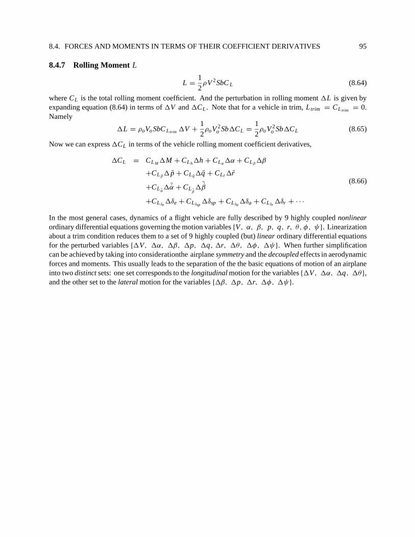
8.4. FORCES AND MOMENTS IN TERMS OF THEIR COEFFICIENT DERIVATIVES 95
8.4.7 Rolling Moment L
L =1
2ρV 2SbC L (8.64)
where CL is the total rolling moment coefficient. And the perturbation in rolling moment 1L is given byexpanding equation (8.64) in terms of 1V and 1CL . Note that for a vehicle in trim, L trim = CL trim = 0.Namely
1L = ρoVo SbC L trim 1V +1
2ρoV 2
o Sb1CL =1
2ρoV 2
o Sb1CL (8.65)
Now we can express 1CL in terms of the vehicle rolling moment coefficient derivatives,
1CL = CL M 1M + CLh1h + CLα1α + CLβ
1β
+CL p1 p + CL q1q + CLr 1r
+CL ¯α1 ¯α + CL ¯β
1 ¯β
+CL δe1δe + CLδsp
1δsp + CLδa1δa + CLδr
1δr + · · ·
(8.66)
In the most general cases, dynamics of a flight vehicle are fully described by 9 highly coupled nonlinearordinary differential equations governing the motion variables {V, α, β, p, q, r, θ, φ, ψ}. Linearizationabout a trim condition reduces them to a set of 9 highly coupled (but) linear ordinary differential equationsfor the perturbed variables {1V, 1α, 1β, 1p, 1q, 1r, 1θ, 1φ, 1ψ}. When further simplificationcan be achieved by taking into considerationthe airplane symmetry and the decoupled effects in aerodynamicforces and moments. This usually leads to the separation of the the basic equations of motion of an airplaneinto two distinct sets: one set corresponds to the longitudinal motion for the variables {1V, 1α, 1q, 1θ},and the other set to the lateral motion for the variables {1β, 1p, 1r, 1φ, 1ψ}.

96 CHAPTER 8. LINEARIZED EQUATIONS OF MOTION

Chapter 9
Linearized Longitudinal Equations of Motion
In this chapter, we examine the flight dynamics characteristics associated with motion in the longitudinalaxis. The assumptions made in the analysis are that the effects of lateral motion on the aerodynamic andpropulsion forces and moments associated with the lift L, drag D and thrust T forces are negligeable. Ofcourse, in the model linearization, wealso assume that the motion of the vehicle is undergoing small changesin the variables 1V , 1α, 1q and 1θ along with small inputs in the controls 1δe, 1δsp and 1δth .
Simple approximation models for the longitudinal dynamics are developed that provide further insightsintothefrequency separationbetween thephugoidandtheshort-periodmodes. Timeresponsesofthe vehiclemotion inthe longitudinalaxis arealsodevelopedillustratingthe effectivenessofthecontrols. Criticaldesignparameters affecting these responses are delineated. Flying qualities of the vehicle are subsequently definedin terms of these fundamental response characteristics.
Following the linearization performed in Chapter 8, the equations of motion governing the longitudinaldynamics are for the motion variables {1V, 1α, 1q, 1θ}. Thus, in general, it is described by a set of 4linear ordinary differential equations obtained from equations (8.18), (8.25) and (8.26). Namely,
1V = −gcos (θo − αo)1θ −Lom 1α − 1
m 1D +cos(αT + αo)
m 1T
1α = 1q −gVo
sin (θo − αo)1θ − DomVo
1α − 1mVo
1L −sin (αT + αo)
mVo1T
1q = 1Iyy
1M
1θ = 1q
(9.1)
The variables θo, αo, Vo, Lo and Do are determined from the trim conditions involving usually the solutionsof a set of nonlinear algebraic equations.
Using expressions for Lo, 1L , Do, 1D and 1T as derived in equations (8.32), (8.33), (8.46), (8.47) and
97

98 CHAPTER 9. LINEARIZED LONGITUDINAL EQUATIONS OF MOTION
(8.53), equations (9.1) become
1V = −gcos (θo − αo)1θ − 1m
12ρoV 2
o SC L(trim )1α − 1m
{ρoVoSC D(trim )1V + 1
2ρoV 2o S
[CDM
a 1V + CDh1h + CDα1α + CDq 1q + CD ¯α
1 ¯α + CDδe1δe + CDδsp
1δsp
]}
+cos(αT + αo)
m12ρoV 2
o S[CTV
1V + CTα1α + CTδth
1δth
]
1α = 1q −gVo
sin (θo − αo)1θ − 1mVo
12ρoV 2
o SC D(trim )1α − 1mVo
{ρoVoSC L(trim )1V
+12ρoV 2
o S[
CLMa 1V + CLh 1h + CLα
1α + CL q 1q + CL ¯α1 ¯α + CLδe
1δe
+CLδsp1δsp
]}−
sin (αT + αo)mVo
12ρoV 2
o S[CTV
1V + CTα1α + CTδth
1δth
]
1q = 1Iyy
12ρoV 2
o Sc[
CMMa 1V + CMh 1h + CMα
1α + CMq 1q + CM ¯α1 ¯α
+CMδe1δe + CMδsp
1δsp
]
1θ = 1q
(9.2)
Foranairplanetrimmedatlevelflight, wehave 1h = 0. Usingthedefinition ofthenondimensionalvariables1V , 1q and 1 ¯α in equations (8.30), we obtain
1 ρoVo Sc4m CD ¯α
0 0
0 1 +ρo Sc4m CL ¯α
0 0
0 −ρoVoSc2
4IyyCM ¯α
1 0
0 0 0 1
1V1α
1q1θ
=
−ρoVo S
2m
(2CD + CDM M − CTV
cos(αT + αo))
−ρoS2m
(2CL + CL M M + CTV
sin(αT + αo))
ρoVo Sc2Iyy
CMM M
0
ρoV 2o S
2m(CL − CDα
+ CTαcos(αT + αo)
) ρoVo Sc4m CDq −g cos(θo − αo)
−ρoVo S
2m(CD + CLα
+ CTαsin(αT + αo)
)1 −
ρo Sc4m CL q −
gVo
sin(θo − αo)
ρoV 2o Sc
2IyyCMα
ρoVoSc2
4IyyCMq 0
0 1 0
1V1α
1q1θ
+
−ρoV 2
o S2m CDδe −
ρoV 2o S
2m CDδsp
ρoV 2o S
2m CTδth cos(αT + αo)
−ρoVo S
2m CLδe −ρoVoS
2m CLδsp −ρoVoS
2m CTδth sin(αT + αo)
ρoV 2o Sc
2IyyCMδe
ρoV 2o Sc
2IyyCMδsp
ρoV 2o Sc
2IyyCMδth
0 0 0
1δe
1δsp
1δth
(9.3)
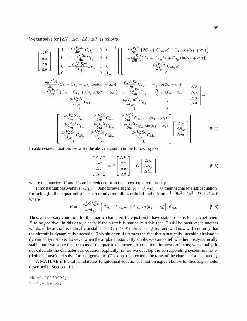
99
We can solve for {1V , 1α, 1q, 1θ} as follows,
1V1α
1q1θ
=
1 ρoVo Sc4m CD ¯α
0 0
0 1 +ρo Sc4m CL ¯α
0 0
0 −ρoVoSc2
4IyyCM ¯α
1 0
0 0 0 1
−1
−ρoVoS
2m
(2CD + CDM M − CTV
cos(αT + αo))
−ρo S2m
(2CL + CLM M + CTV
sin(αT + αo))
ρoVoSc2Iyy
CMM M
0
ρoV 2o S
2m(CL − CDα
+ CTαcos(αT + αo)
) ρoVo Sc4m CDq −g cos(θo − αo)
−ρoVo S
2m(CD + CLα
+ CTαsin(αT + αo)
)1 −
ρo Sc4m CL q −
gVo
sin(θo − αo)
ρoV 2o Sc
2IyyCMα
ρoVoSc2
4IyyCMq 0
0 1 0
1V1α
1q1θ
+
−ρoV 2
o S2m CDδe −
ρoV 2o S
2m CDδsp
ρoV 2o S
2m CTδth cos(αT + αo)
−ρoVoS
2m CLδe −ρoVoS
2m CL δsp −ρoVoS
2m CTδth sin(αT + αo)
ρoV 2o Sc
2IyyCMδe
ρoV 2o Sc
2IyyCMδsp
ρoV 2o Sc
2IyyCMδth
0 0 0
1δe
1δsp
1δth
(9.4)
In abbreviated notation, we write the above equation in the following form
1V1α
1q1θ
= F
1V1α
1q1θ
+ G
1δe
1δsp
1δth
(9.5)
where the matrices F and G can be deduced from the above equation directly.Inmostsituations,wehave CMM = 0andforlevelflight γo = θo−αo = 0, thenthecharacteristicequation
forthelongitudinalequationisa4 th -orderpolynomialin s ofthefollowingform s4+Bs 3+Cs 2+Ds +E = 0where
E = −ρ2
o S2V 2o c
4mI yy
{2CL + CL M M + CTV
sin (αT + αo)}
gC Mα(9.6)
Thus, a necessary condition for the quartic characteristic equation to have stable roots is for the coefficientE to be positive. In this case, clearly if the aircraft is statically stable then E will be positive; in anotherwords, if the aircraft is statically unstable (i.e. CMα
≥ 0) then E is negative and we know with certainty thatthe aircraft is dynamically unstable. This situation illustrates the fact that a statically unstable airplane isdynamicallyunstable; howeverwhen the airplane isstatically stable, we cannot tell whether it isdynamicallystable until we solve for the roots of the quartic characteristic equation. In most problems, we actually donot calculate the characteristic equation explicitly, rather we develop the corresponding system matrix F(defined above) and solve for its eigenvalues (They are then exactly the roots of the characteristic equation).
A MATLAB-mfile toformulatethe longitudinal equationsof motion isgiven below for thedesign modeldescribed in Section 11.1.
rho=0.00230990;Vo=556.29559;

100 CHAPTER 9. LINEARIZED LONGITUDINAL EQUATIONS OF MOTION
S=608;c=15.95;b=42.8;Ixx=28700;Iyy=165100;Izz=187900;Izx=-520;Ixy=0;Iyz=0;M=0.5;CL=0.20709;CD=0.01468;g=32.17095;Weight=45000;m=Weight/g;%Lift Coefficient DerivativesCLq=-17.2322;CLM=7.45058e-6;CLalpha=4.8706;CLalphadot=17.2322;CLelev=0.572957;%Drag Coefficient DerivativesCDq=0;CDM=0;CDalpha=0.37257;CDalphadot=0;CDelev=4.38308e-2;%Pitch Moment Coefficient DerivativesCMq=3.8953;CMM=-7.05586e-6;CMalpha=-0.168819;CMalphadot=-11.887;CMelev=-0.695281;%Thrust Coefficient DerivativesCTv=0;CTalpha=0;alphaT=0;%Trim angle of attackalphao=0.18105*pi/180;thetao=alphao;%Matrix AA=[1,rho*Vo*S*c*CDalphadot/4/m,0,0;
0,1+rho*S*c*CLalphadot/4/m,0,0;0,-rho*Vo*S*c^2*CMalphadot/4/Iyy,1,0;0,0,0,1];
B1=[-rho*Vo*S/2/m*(2*CD+CDM*M-CTv*cos(alphaT+alphao));-rho*S/2/m*(2*CL+CLM*M+CTv*sin(alphaT+alphao));
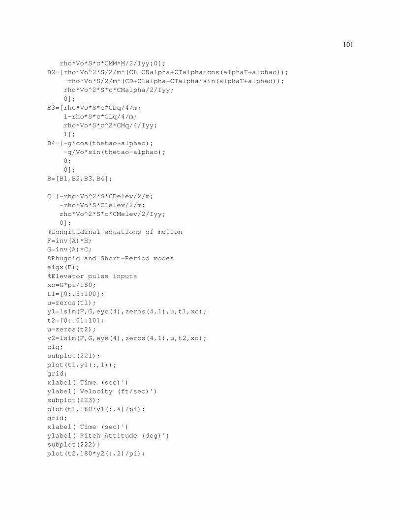
101
rho*Vo*S*c*CMM*M/2/Iyy;0];B2=[rho*Vo^2*S/2/m*(CL-CDalpha+CTalpha*cos(alphaT+alphao));
-rho*Vo*S/2/m*(CD+CLalpha+CTalpha*sin(alphaT+alphao));rho*Vo^2*S*c*CMalpha/2/Iyy;0];
B3=[rho*Vo*S*c*CDq/4/m;1-rho*S*c*CLq/4/m;rho*Vo*S*c^2*CMq/4/Iyy;1];
B4=[-g*cos(thetao-alphao);-g/Vo*sin(thetao-alphao);0;0];
B=[B1,B2,B3,B4];
C=[-rho*Vo^2*S*CDelev/2/m;-rho*Vo*S*CLelev/2/m;rho*Vo^2*S*c*CMelev/2/Iyy;0];
%Longitudinal equations of motionF=inv(A)*B;G=inv(A)*C;%Phugoid and Short-Period modeseigx(F);%Elevator pulse inputsxo=G*pi/180;t1=[0:.5:100];u=zeros(t1);y1=lsim(F,G,eye(4),zeros(4,1),u,t1,xo);t2=[0:.01:10];u=zeros(t2);y2=lsim(F,G,eye(4),zeros(4,1),u,t2,xo);clg;subplot(221);plot(t1,y1(:,1));grid;xlabel('Time (sec)')ylabel('Velocity (ft/sec)')subplot(223);plot(t1,180*y1(:,4)/pi);grid;xlabel('Time (sec)')ylabel('Pitch Attitude (deg)')subplot(222);plot(t2,180*y2(:,2)/pi);

102 CHAPTER 9. LINEARIZED LONGITUDINAL EQUATIONS OF MOTION
grid;xlabel('Time (sec)')ylabel('Angle of Attack (deg)')subplot(224);plot(t2,180*y2(:,3)/pi);grid;xlabel('Time (sec)')ylabel('Pitch Rate (deg/sec)')pause%Short-period approximation: Delete the velocity and theta equationsFsp=F(2:3,2:3);Gsp=G(2:3,1);damp(Fsp);%Elevator pulse inputsxo=Gsp*pi/180;t1=[0:.01:10];u=zeros(t1);y1=lsim(Fsp,Gsp,eye(2),zeros(2,1),u,t1,xo);clg;subplot(211);plot(t1,y1(:,1));grid;xlabel('Time (sec)')ylabel('Angle of Attack (deg)')subplot(212);plot(t1,180*y1(:,2)/pi);grid;xlabel('Time (sec)')ylabel('Pitch Rate (deg/sec)')pause%Phugoid approximationfreqphg=g/Vo*sqrt(2)
Running this MATLAB m-file generates the following longitudinal models:
1V1α
1q1θ
= F
1V1α
1q1θ
+ G1δe (9.7)
where the matrices F and G are given by
F =-8.1994e-03 -2.5708e+01 0 -3.2171e+01-1.9451e-04 -1.2763e+00 1.0000e+00 06.9573e-04 1.0218e+00 -2.4052e+00 0
0 0 1.0000e+00 0

9.1. PHUGOID-MODE APPROXIMATION 103
G =-6.8094e+00-1.4968e-01-1.4061e+01
0
Characteristic roots of the longitudinal model are given by the eigenvalues of the system matrix F. This canbe calculated using the MATLAB function damp(F).
Eigenvalues Damping Frequency(rad/sec)-0.0012693 0.10392i 0.012 0.10392 (Phugoid mode)-0.0012693 -0.10392i 0.012 0.10392 (Phugoid mode)-0.68348 0i 1.000 0.68348 (Short-Period mode)-3.0037 0i 1.000 3.0037 (Short-Period mode)
where the damping ratio ζ of a complex root (s = σ + jω) is defined as follows
ζ =−σ
√σ 2 + ω2
Notice that −1 ≤ ζ ≤ 1. A negative damping ratio means that the motion is dynamically unstable.In most longitudinal aircraft motion, we can distinguish two basic modes: the phugoid mode and the
short-period mode. The phugoid mode is the one that has the longest time constant and is usually lightlydamped. Responses of the aircraft that are significantly affected by the phugoid mode are the velocity andthe pitch attitude as seen in Fig. 9.1 . There is very little response seen in the angle of attack 1α whenthe aircraft is excited in the phugoid mode. Note that the period of the velocity 1V and pitch attitude1q responses is roughly equal to the period of the phugoid mode determined from the approximationTphugoid =
√2πVo/g =
√2π556.29559/32.17095 = 76.8(sec) as discussed in Section 9.1. Damping
of the phugoid mode is predominantly governed by the drag coefficient CD and its derivative CDM in theequation for 1V . More precisely, the term (2CD + CDM M) or (2CD + CDV Vo) is the damping factor in thespeed equation.
The short-period mode is displayed in the motion of the airplane angle of attack 1α and pitch rate 1q(Fig. 9.1). It has a relatively short time constant (hence the name short-period). In most situation, this modeis relatively well damped (if not, then one must provide stabilization of thismodes using feedback control forflight safety since the pilot cannot control this mode). Theshort-period mode is usuallyidentified by a pair ofcomplex roots, but in some flight conditions it can be in terms of two real roots as seen in the above exampleproblem where s3 = −0.68 rad/sec and s4 = −3.0 rad/sec. In some control design problems, one would liketo obtain a simplified second-order dynamic model for the longitudinal aircraft motion that captures the fastmotion (i.e. the short-period mode) only.
9.1 Phugoid-Mode Approximation
The phugoid frequency ωphugoid in a level-flight trim condition (i.e. γo = θo − αo = 0) can be estimatedfrom the speed and pitch attitude equations where we neglect the variation in 1α (i.e. 1α = 0) and the drageffects. Furthermore, we assume CTV
= 0 and CTα= 0 and for a fixed elevator 1δe = 0. In this case, the

104 CHAPTER 9. LINEARIZED LONGITUDINAL EQUATIONS OF MOTION
-50
0
50
0 50 100
Time (sec)
Vel
ocity
(ft
/sec
)
-10
0
10
0 50 100
Time (sec)
Pitc
h A
ttitu
de (
deg)
-4
-2
0
2
0 5 10
Time (sec)
Ang
le o
f A
ttack
(de
g)
-20
-10
0
10
0 5 10
Time (sec)
Pitc
h R
ate
(deg
/sec
)
Figure 9.1: Longitudinal Aircraft Responses to a 1-deg Elevator Impulsive Input
motion of the airplane is governed entirely by the exchange of kinetic and potential energies. And we have
1V = −g1θ
1α = 0 = 1q −ρoSC L
m 1V
1θ = 1q =ρo SCL
m 1V
(9.8)
or [1V1θ
]=
[0 −g
ρoSC Lm 0
] [1V1θ
](9.9)
Characteristic equation of the above equation is simply equal to
det[
s g
−ρo SC L
m s
]= s2 +
ρogSC L
m= s2 + 2
g2
V 2o
= 0 (9.10)
with characteristicroots at s1,2 = ± j√
2g/Vo which correspondtosinusoidal motions inthe aircraftvelocityand pitch attitude. Thus, the phugoid mode frequency should be roughly equal to ωphugoid =
√2g/Vo
(rad/sec).Applyingtothegivennumericalexample, wehave ωphugoid = 0.0818rad/secwithaperiodof Tphugoid =
2π/ωphugoid = 76.8 sec.Another interpretation of the phugoid oscillation is as follows. The motion exhibited in the phugoid
mode typifies the exchange of potential and kinetic energies of the aircraft. Recall that when the airplane istreated as a point mass m, the total energy is given by
1
2mV 2 + mgh = constant (9.11)
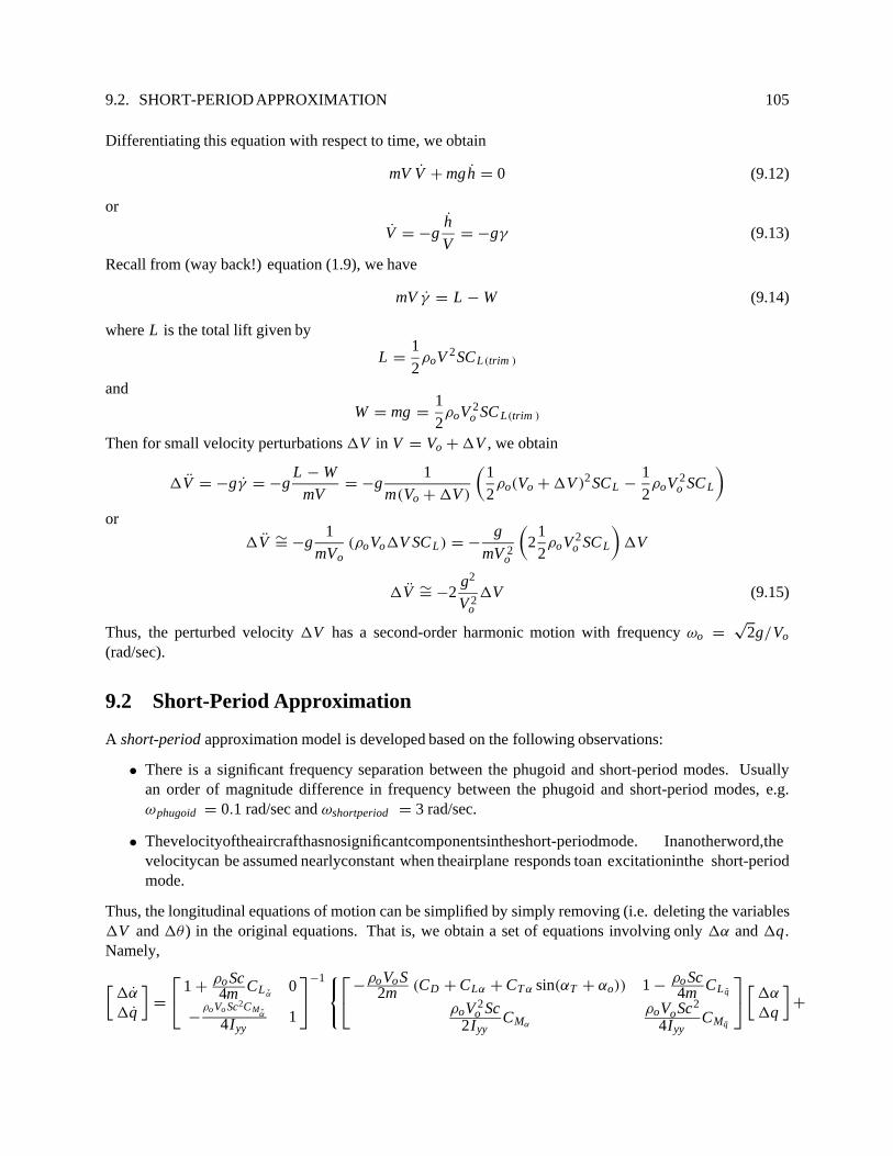
9.2. SHORT-PERIOD APPROXIMATION 105
Differentiating this equation with respect to time, we obtain
mV V + mgh = 0 (9.12)
or
V = −gh
V= −gγ (9.13)
Recall from (way back!) equation (1.9), we have
mV γ = L − W (9.14)
where L is the total lift given by
L =1
2ρoV 2SCL(trim )
and
W = mg =1
2ρoV 2
o SC L(trim )
Then for small velocity perturbations 1V in V = Vo + 1V , we obtain
1V = −gγ = −gL − W
mV= −g
1m(Vo + 1V )
(12ρo(Vo + 1V )2 SCL −
12ρoV 2
o SC L
)
or
1V ∼= −g1
mVo(ρoVo1V SC L) = −
g
mV 2o
(2
12ρoV 2
o SC L
)1V
1V ∼= −2g2
V 2o
1V (9.15)
Thus, the perturbed velocity 1V has a second-order harmonic motion with frequency ωo =√
2g/Vo
(rad/sec).
9.2 Short-Period Approximation
A short-period approximation model is developed based on the following observations:
• There is a significant frequency separation between the phugoid and short-period modes. Usuallyan order of magnitude difference in frequency between the phugoid and short-period modes, e.g.ωphugoid = 0.1 rad/sec and ωshortperiod = 3 rad/sec.
• Thevelocityoftheaircrafthasnosignificantcomponentsintheshort-periodmode. Inanotherword,thevelocitycan be assumed nearlyconstant when theairplane responds toan excitationinthe short-periodmode.
Thus, the longitudinal equations of motion can be simplified by simply removing (i.e. deleting the variables1V and 1θ ) in the original equations. That is, we obtain a set of equations involving only 1α and 1q.Namely,
[1α
1q
]=
1 +ρo Sc4m CL ¯α
0
−ρoVo Sc2CM ¯α
4Iyy1
−1
−ρoVo S
2m (CD + CLα + CT α sin(αT + αo)) 1 −ρo Sc4m CL q
ρoV 2o Sc
2IyyCMα
ρoVoSc2
4IyyCMq
[1α
1q
]+

106 CHAPTER 9. LINEARIZED LONGITUDINAL EQUATIONS OF MOTION
−ρoVo S
2m CLδe −ρoVo S
2m CL δsp −ρoVo S
2m CT δth cos(αT + αo)
ρoV 2o Sc
2IyyCMδe
ρoV 2o Sc
2IyyCMδsp
ρoV 2o Sc
2IyyCMδth
1δe
1δsp
1δth
(9.16)
For the above problem, we obtain the following short-period approximation model[1α
1q
]=
[−1.2763 11.0218 −2.4052
] [1α(rad )
1q
]+
[−0.1497−14.0611
]1δe (9.17)
where 1α, 1δe are in radians and 1q in radians/sec. Characteristic roots of the short-period model are givenbelow. They are almost the same as those obtained in the full (4th -order) longitudinal model.
Eigenvalues Damping Frequency(rad/sec)-0.68299 1.000 0.68299-2.9985 1.000 2.9985
Figure 9.2 shows the responses of the short-period approximation model to a 1-deg elevator impulseinput. Note that these responses of 1α and 1q match closely those obtained for the full (i.e. 4th -order)
longitudinal model. In general, CLα>> CD , CTα
≈ 0 andρo ScC L q
4m << 1, then the above short-periodapproximation has the following characteristic equation
s2 +ρoVo Sc2
2Iyy
(Iyy CLα
mc2−
1
2CMq
)s +
ρoV 2o Sc
2IyyCLα
(−
CMα
CLα
−ρSc
4mCMq
)= 0 (9.18)
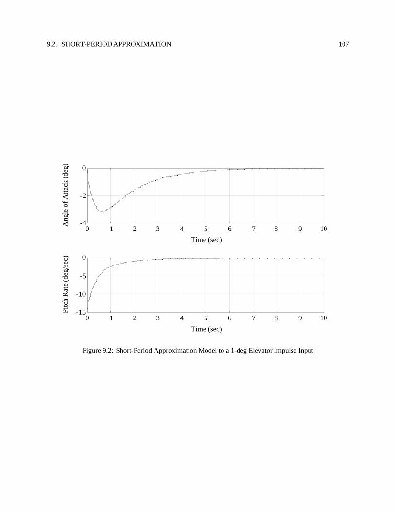
9.2. SHORT-PERIOD APPROXIMATION 107
-4
-2
0
0 1 2 3 4 5 6 7 8 9 10
Time (sec)
Ang
le o
f A
ttack
(de
g)
-15
-10
-5
0
0 1 2 3 4 5 6 7 8 9 10
Time (sec)
Pitc
h R
ate
(deg
/sec
)
Figure 9.2: Short-Period Approximation Model to a 1-deg Elevator Impulse Input

108 CHAPTER 9. LINEARIZED LONGITUDINAL EQUATIONS OF MOTION

Chapter 10
Linearized Lateral Equations of Motion
In this chapter, we examine the flight dynamics characteristics associated with motion in the lateral axis.The assumptions made in the analysis are that the effects of longitudinal motion on the aerodynamic andpropulsion forces and moments associated with the lift L , drag D and thrust T forces are negligeable.Hence, the motion in the lateral axis is decoupled from the longitudinal dynamics. Of course, in any modellinearization, we also assume that the motion of the vehicle is undergoing small changes in the variables 1β ,1p, 1r and 1φ along with small inputs in the controls 1δa and 1δr .
Equationsgoverningthelateralmotionofanaircraftareassociatedwiththemotionvariables 1β, 1p, 1r, 1φ.Hence, the lateral dynamic model is described by a set of 4 linear ordinary differential equations as derivedin equations (8.18), (8.25) and (8.28). Namely,
1β = sin αo1p − cos αo1r +gVo
cos θo1φ + 1mVo
1Y[
Ixx −Ixz
−Izx Izz
] [1 p1r
]=
[1L1N
]
1φ = 1p + tan θo1r
(10.1)
Using equations (8.50), (8.65) and (8.62) for 1Y , 1L and 1N , and retaining only the contributions due tolateral motion variables, we obtain
• Sideslip equation for 1β:
1β = sin αo1p − cos αo1r +g
Vocos θo1φ
+1
mVo
1
2ρoV 2
o S(
CYβ1β + CY p1 p + CYr 1r + CY ¯β
1 ¯β+CYδa1δa + CYδr 1δr
)(10.2)
or (1 −
1
mVoCY ¯β
b
2Vo
)1β = sin αo1p − cos αo1r +
g
Vocos θo1φ
+1
mVo
1
2ρoV 2
o S(CYβ
1β + CY p1 p + CYr 1r + CYδa1δa + CYδr 1δr
)(10.3)
Dividing by (1 − b2mV 2
oCY ¯β
), we obtain
1β =1
1 − b2mV 2
oCY ¯β
{ρoVoS
2mCYβ
1β +
(sin αo +
ρobS
4mCY p
)1p
109
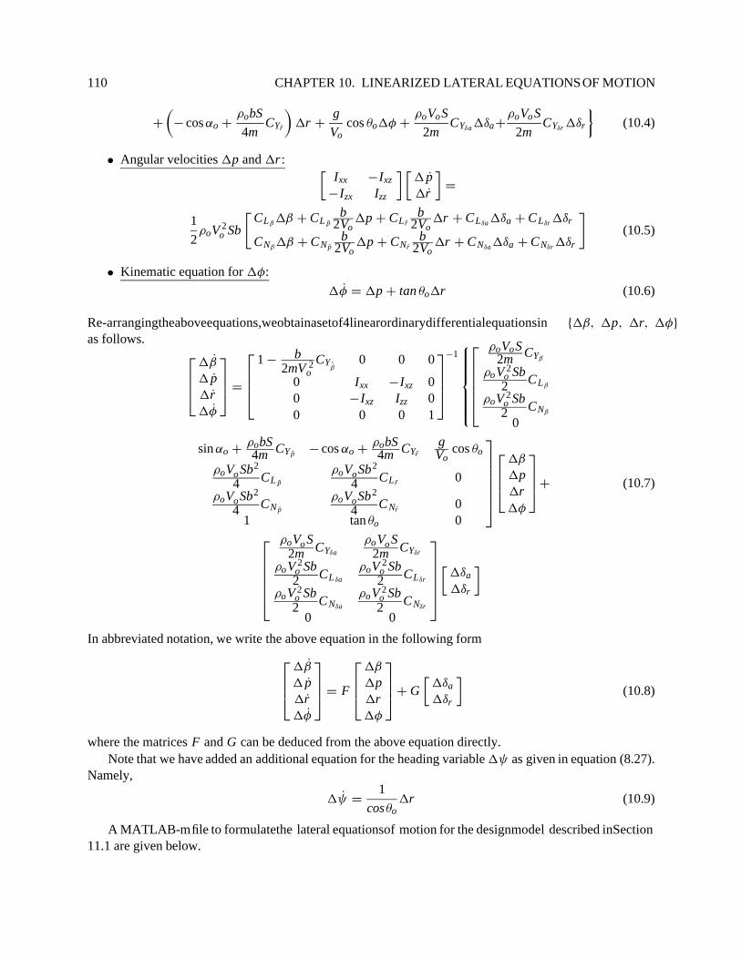
110 CHAPTER 10. LINEARIZED LATERAL EQUATIONS OF MOTION
+
(− cos αo +
ρobS
4mCYr
)1r +
g
Vocos θo1φ +
ρoVoS
2mCYδa1δa+
ρoVo S
2mCYδr 1δr
}(10.4)
• Angular velocities 1p and 1r : [Ixx −Ixz
−Izx Izz
] [1 p1r
]=
1
2ρoV 2
o Sb
[CLβ
1β + CL pb
2Vo1p + CL r
b2Vo
1r + CLδa1δa + CLδr 1δr
CNβ1β + CN p
b2Vo
1p + CNrb
2Vo1r + CNδa1δa + CNδr 1δr
](10.5)
• Kinematic equation for 1φ:
1φ = 1p + tan θo1r (10.6)
Re-arrangingtheaboveequations,weobtainasetof4linearordinarydifferentialequationsin {1β, 1p, 1r, 1φ}
as follows.
1β
1 p1r1φ
=
1 − b2mV 2
oCY ¯β
0 0 0
0 Ixx −Ixz 00 −Ixz Izz 00 0 0 1
−1
ρoVoS2m CYβ
ρoV 2o Sb2 CLβ
ρoV 2o Sb2 CNβ
0
sin αo +ρobS4m CY p − cos αo +
ρobS4m CYr
gVo
cos θo
ρoVo Sb2
4 CL p
ρoVoSb2
4 CL r 0
ρoVoSb2
4 CN p
ρoVoSb2
4 CNr 01 tan θo 0
1β
1p1r1φ
+ (10.7)
ρoVo S2m CYδa
ρoVo S2m CYδr
ρoV 2o Sb2 CL δa
ρoV 2o Sb2 CLδr
ρoV 2o Sb2 CNδa
ρoV 2o Sb2 CNδr
0 0
[1δa
1δr
]
In abbreviated notation, we write the above equation in the following form
1β
1 p1r1φ
= F
1β
1p1r1φ
+ G
[1δa
1δr
](10.8)
where the matrices F and G can be deduced from the above equation directly.Note that we have added an additional equation for the heading variable 1ψ as given in equation (8.27).
Namely,
1ψ =1
cosθo1r (10.9)
A MATLAB-mfile to formulatethe lateral equationsof motion for the designmodel described inSection11.1 are given below.

111
clg;clear;rho=0.00230990;Vo=556.29559;S=608;c=15.95;b=42.8;Ixx=28700;Iyy=165100;Izz=187900;Izx=-520;Ixy=0;Iyz=0;M=0.5;CL=0.20709;CD=0.01468;g=32.17095;Weight=45000;m=Weight/g;%Side Force Coefficient DerivativesCYp=0;CYr=0;CYbeta=-0.97403;CYbetadot=0;CYrud=-1.5041e-1;CYail=-1.1516e-3;%Yawing Moment Coefficient DerivativesCNp=-3.3721e-2;CNr=-4.0471e-1;CNbeta=1.2996e-1;CNrud=-6.9763e-2;CNail=2.1917e-3;%Rolling Moment Coefficient DerivativesCLp=-0.2;CLr=0.15099;CLbeta=-0.13345;CLrud=-2.3859e-3;CLail=2.6356e-2;%Trim angle of attackalphao=0.18105*pi/180;thetao=alphao;%Matrix AA=[1-b*CYbetadot/(2*m*Vo^2),0,0,0
0,Ixx,-Izx,00,-Izx,Izz,00,0,0,1];
B1=[rho*Vo*S*CYbeta/2/m;0.5*rho*Vo^2*S*b*CLbeta;

112 CHAPTER 10. LINEARIZED LATERAL EQUATIONS OF MOTION
0.5*rho*Vo^2*S*b*CNbeta;0];B2=[sin(alphao)+rho*b*S*CYp/4/m;
0.25*rho*Vo*S*b^2*CLp;0.25*rho*Vo*S*b^2*CNp;1];
B3=[-cos(alphao)+rho*b*S*CYr/4/m;0.25*rho*Vo*S*b^2*CLr;0.25*rho*Vo*S*b^2*CNr;tan(thetao)];
B4=[g/Vo*cos(thetao);0;0;0];
B=[B1,B2,B3,B4];C=[rho*Vo*S*CYail/2/m, rho*Vo*S*CYrud/2/m;
0.5*rho*Vo^2*S*b*CLail, 0.5*rho*Vo^2*S*b*CLrud;0.5*rho*Vo^2*S*b*CNail, 0.5*rho*Vo^2*S*b*CNrud;0,0];
%Lateral equations of motionF=inv(A)*B;G=inv(A)*C;%Add the heading equationFx=[[F,zeros(4,1)];[0,0,1/cos(thetao),0,0]];Gx=[G;[0,0]];%Dutch roll, spiral and roll modeseigx(F);eigx(Fx);%Aileron pulse inputsxo=-Gx(:,1)*pi/180; %Switch sign for + right aileron downt1=[0:.1:30];u=zeros(t1);y1=lsim(Fx,Gx(:,1),eye(5),zeros(5,1),u,t1,xo);clg;subplot(221);plot(t1,180*y1(:,1)/pi);grid;xlabel('Time (sec)')ylabel('Sideslip (deg)')title('Aileron 1-deg Pulse Input')subplot(223);plot(t1,180*y1(:,2)/pi);grid;xlabel('Time (sec)')ylabel('Roll Rate (deg/sec)')subplot(222);

113
plot(t1,180*y1(:,3)/pi);grid;xlabel('Time (sec)')ylabel('Yaw Rate (deg/sec)')subplot(224);plot(t1,180*y1(:,4)/pi,t1,180*y1(:,5)/pi);grid;xlabel('Time (sec)')ylabel('Roll/Heading Angles (deg)')pause%Rudder pulse inputsxo=Gx(:,2)*pi/180;t1=[0:.1:30];u=zeros(t1);y1=lsim(Fx,Gx(:,2),eye(5),zeros(5,1),u,t1,xo);clg;subplot(221);plot(t1,180*y1(:,1)/pi);grid;xlabel('Time (sec)')ylabel('Sideslip (deg)')title('Rudder 1-deg Pulse Input')subplot(223);plot(t1,180*y1(:,2)/pi);grid;xlabel('Time (sec)')ylabel('Roll Rate (deg/sec)')subplot(222);plot(t1,180*y1(:,3)/pi);grid;xlabel('Time (sec)')ylabel('Yaw Rate (deg/sec)')subplot(224);plot(t1,180*y1(:,4)/pi,t1,180*y1(:,5)/pi);grid;xlabel('Time (sec)')ylabel('Roll/Heading Angles (deg)')
Running this MATLAB m-file generates the following linearized lateral dynamic model:
1β
1 p1r1φ
1ψ
= Fp
1β
1p1r1φ
1ψ
+ G p
[1δa
1δr
](10.10)
where the matrices Fp and G p are given by
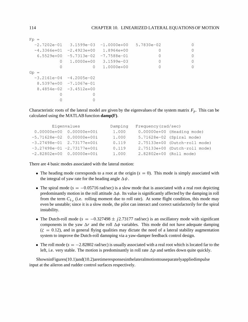
114 CHAPTER 10. LINEARIZED LATERAL EQUATIONS OF MOTION
Fp =-2.7202e-01 3.1599e-03 -1.0000e+00 5.7830e-02 0-4.3366e+01 -2.4923e+00 1.8964e+00 0 06.5529e+00 -5.7313e-02 -7.7588e-01 0 0
0 1.0000e+00 3.1599e-03 0 00 0 1.0000e+00 0 0
Gp =-3.2161e-04 -4.2005e-028.5397e+00 -7.1067e-018.4854e-02 -3.4512e+00
0 00 0
Characteristic roots of the lateral model are given by the eigenvalues of the system matrix Fp. This can becalculated using the MATLAB function damp(F).
Eigenvalues Damping Frequency(rad/sec)0.00000e+00 0.00000e+00i 1.000 0.00000e+00 (Heading mode)-5.71628e-02 0.00000e+00i 1.000 5.71628e-02 (Spiral mode)-3.27498e-01 2.73177e+00i 0.119 2.75133e+00 (Dutch-roll mode)-3.27498e-01 -2.73177e+00i 0.119 2.75133e+00 (Dutch-roll mode)-2.82802e+00 0.00000e+00i 1.000 2.82802e+00 (Roll mode)
There are 4 basic modes associated with the lateral motion:
• The heading mode corresponds to a root at the origin (s = 0). This mode is simply associated withthe integral of yaw rate for the heading angle 1ψ .
• The spiral mode (s = −0.05716 rad/sec) is a slow mode that is associated with a real root depictingpredominantly motion in the roll attitude 1φ. Its value is significantly affected by the damping in rollfrom the term CL p (i.e. rolling moment due to roll rate). At some flight condition, this mode mayeven be unstable; since it is a slow mode, the pilot can interact and correct satisfactorily for the spiralinstability.
• The Dutch-roll mode (s = −0.327498 ± j2.73177 rad/sec) is an oscillatory mode with significantcomponents in the yaw 1r and the roll 1φ variables. This mode did not have adequate damping(ζ = 0.12), and in general flying qualities may dictate the need of a lateral stability augmentationsystem to improve the Dutch-roll damnping via a yaw-damper feedback control design.
• The roll mode (s = −2.82802 rad/sec) is usually associated with a real root which is located far to theleft, i.e. very stable. The motion is predominantly in roll rate 1p and settles down quite quickly.
ShowninFigures(10.1)and(10.2)aretimeresponsesinthelateralmotiontoaseparatelyappliedimpulseinput at the aileron and rudder control surfaces respectively.

115
-0.1
-0.05
0
0.05
0 10 20 30
Time (sec)
Side
slip
(de
g)
Aileron 1-deg Pulse Input
-10
-5
0
5
0 10 20 30
Time (sec)
Rol
l Rat
e (d
eg/s
ec)
-0.3
-0.2
-0.1
0
0.1
0 10 20 30
Time (sec)
Yaw
Rat
e (d
eg/s
ec)
-3
-2
-1
0
0 10 20 30
Time (sec)
Rol
l/Hea
ding
Ang
les
(deg
)
Figure 10.1: Lateral Responses to a 1-deg Aileron Impulse Input

116 CHAPTER 10. LINEARIZED LATERAL EQUATIONS OF MOTION
-1
-0.5
0
0.5
1
0 10 20 30
Time (sec)
Side
slip
(de
g)
Rudder 1-deg Pulse Input
-15
-10
-5
0
5
10
0 10 20 30
Time (sec)
Rol
l Rat
e (d
eg/s
ec)
-4
-2
0
2
0 10 20 30
Time (sec)
Yaw
Rat
e (d
eg/s
ec)
-15
-10
-5
0
5
0 10 20 30
Time (sec)
Rol
l/Hea
ding
Ang
les
(deg
)
Figure 10.2: Lateral Responses to a 1-deg Rudder Impulse Input

Chapter 11
Flight Vehicle Models
11.1 Generic F-15 Model Data (Subsonic)
WING AREA 608.000 (FT**2)WING SPAN 42.800 (FT)MEAN CHORD 15.950 (FT)VEHICLE WEIGHT 45000.000 (LB)IXX 28700.000 (SLUG-FT**2)IYY 165100.000 (SLUG-FT**2)IZZ 187900.000 (SLUG-FT**2)IXZ -520.000 (SLUG-FT**2)IXY 0.000 (SLUG-FT**2)IYZ 0.000 (SLUG-FT**2)
COEFFICIENT OF LIFT = 0.20709COEFFICIENT OF DRAG = 0.01468LIFT (LBS) = 45001.75037DRAG (LBS) = 3190.16917ALTITUDE (FT) = 1000.MACH = 0.50000VELOCITY (FT/SEC) = 556.29559EQUIVALENT AIRSPEED (KTS) = 324.60706SPEED OF SOUND (FT/SEC) = 1112.59123GRAVITATIONAL ACCEL (FT/SEC**2) = 32.17095NORMAL ACCELERATION (G-S) = 1.00026LOAD FACTOR = 1.00013DYNAMIC PRESSURE (LBS/FT**2) = 357.41711DENSITY (SLUG/FT**3) = 0.00230990WEIGHT (@ALTITUDE) (LBS) = 44995.73786BETA (DEG) = 0.00000ALPHA (DEG) = 0.18105PHI (DEG) = 0.00000THETA (DEG) = 0.18105ALTITUDE RATE (FT/SEC) = 0.00000GAMMA (DEG) = 0.00000ROLL RATE (DEG/SEC) = 0.00000PITCH RATE (DEG/SEC) = 0.00000
117
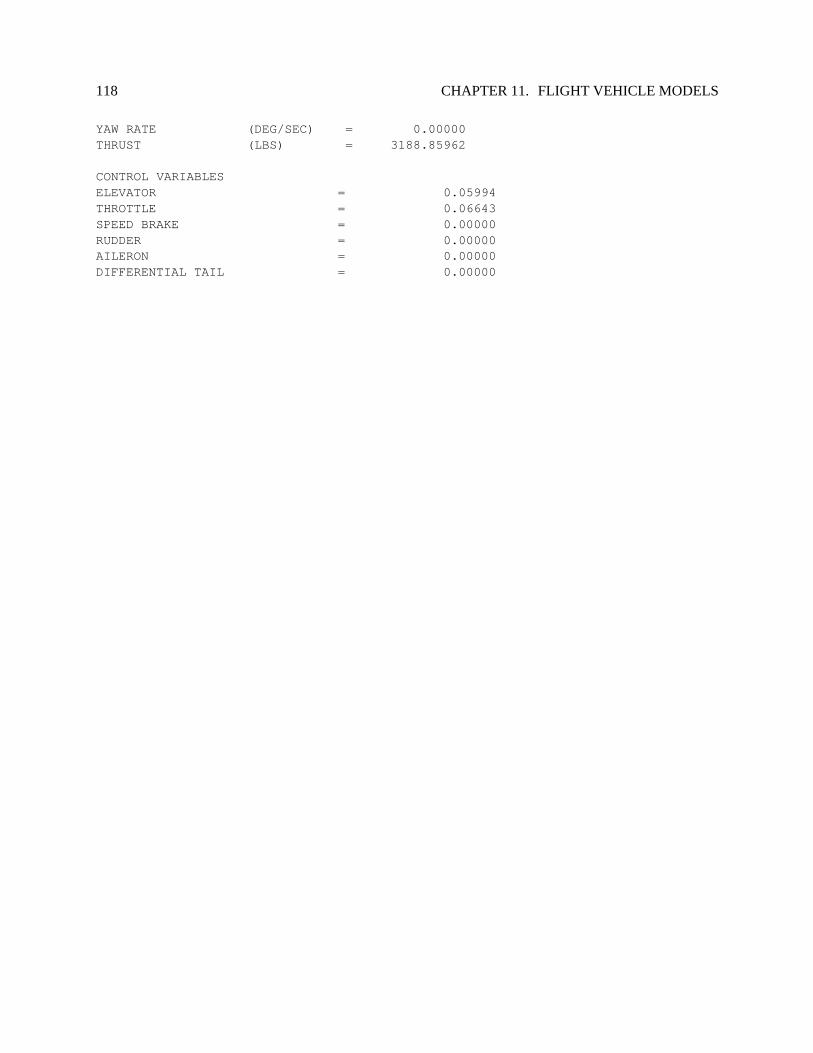
118 CHAPTER 11. FLIGHT VEHICLE MODELS
YAW RATE (DEG/SEC) = 0.00000THRUST (LBS) = 3188.85962
CONTROL VARIABLESELEVATOR = 0.05994THROTTLE = 0.06643SPEED BRAKE = 0.00000RUDDER = 0.00000AILERON = 0.00000DIFFERENTIAL TAIL = 0.00000

11.1. GENERIC F-15 MODEL DATA(SUBSONIC) 119
NON-DIMENSIONAL STABILITY AND CONTROL DERIVATIVES
SIDEDRAG LIFT FORCE________ ________ ________
ZERO COEFFICIENTS 1.08760D-02 1.57360D-01 2.12070D-18
ROLL RATE 0.00000D+00 0.00000D+00 0.00000D+00PITCH RATE 0.00000D+00 -1.72322D+01 0.00000D+00YAW RATE 0.00000D+00 0.00000D+00 0.00000D+00MACH NUMBER 0.00000D+00 7.45058D-06 0.00000D+00ALPHA (RAD) 3.72570D-01 4.87060D+00 0.00000D+00BETA (RAD) 0.00000D+00 0.00000D+00 -9.74030D-01ALTITUDE (FT) 0.00000D+00 0.00000D+00 0.00000D+00ALPHA DOT 0.00000D+00 1.72322D+01 0.00000D+00BETA DOT 0.00000D+00 0.00000D+00 0.00000D+00
ELEVATOR 4.38308D-02 5.72957D-01 0.00000D+00SPEED BRAKE 6.49346D-02 3.74913D-02 0.00000D+00RUDDER 0.00000D+00 0.00000D+00 -1.50410D-01AILERON 0.00000D+00 0.00000D+00 -1.15160D-03DIFFERENTIAL TAIL 0.00000D+00 0.00000D+00 -7.93150D-02
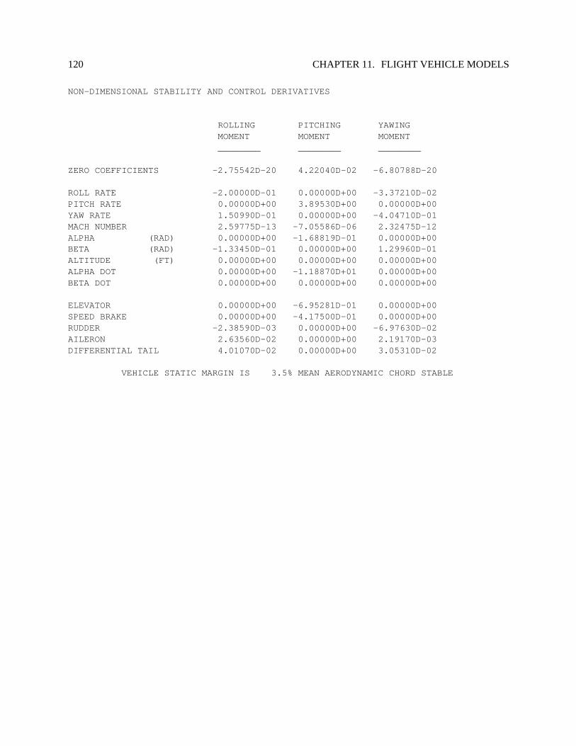
120 CHAPTER 11. FLIGHT VEHICLE MODELS
NON-DIMENSIONAL STABILITY AND CONTROL DERIVATIVES
ROLLING PITCHING YAWINGMOMENT MOMENT MOMENT________ ________ ________
ZERO COEFFICIENTS -2.75542D-20 4.22040D-02 -6.80788D-20
ROLL RATE -2.00000D-01 0.00000D+00 -3.37210D-02PITCH RATE 0.00000D+00 3.89530D+00 0.00000D+00YAW RATE 1.50990D-01 0.00000D+00 -4.04710D-01MACH NUMBER 2.59775D-13 -7.05586D-06 2.32475D-12ALPHA (RAD) 0.00000D+00 -1.68819D-01 0.00000D+00BETA (RAD) -1.33450D-01 0.00000D+00 1.29960D-01ALTITUDE (FT) 0.00000D+00 0.00000D+00 0.00000D+00ALPHA DOT 0.00000D+00 -1.18870D+01 0.00000D+00BETA DOT 0.00000D+00 0.00000D+00 0.00000D+00
ELEVATOR 0.00000D+00 -6.95281D-01 0.00000D+00SPEED BRAKE 0.00000D+00 -4.17500D-01 0.00000D+00RUDDER -2.38590D-03 0.00000D+00 -6.97630D-02AILERON 2.63560D-02 0.00000D+00 2.19170D-03DIFFERENTIAL TAIL 4.01070D-02 0.00000D+00 3.05310D-02
VEHICLE STATIC MARGIN IS 3.5% MEAN AERODYNAMIC CHORD STABLE
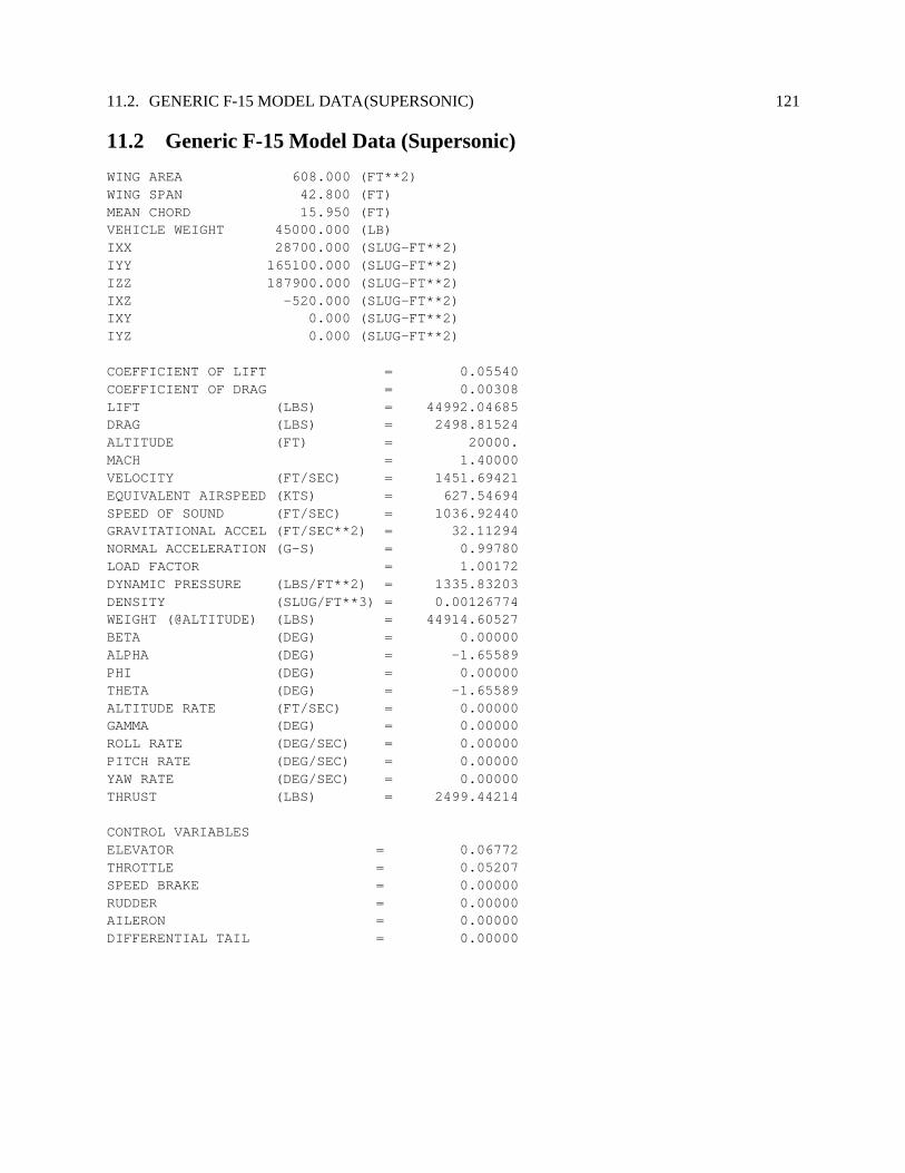
11.2. GENERIC F-15 MODEL DATA(SUPERSONIC) 121
11.2 Generic F-15 Model Data (Supersonic)
WING AREA 608.000 (FT**2)WING SPAN 42.800 (FT)MEAN CHORD 15.950 (FT)VEHICLE WEIGHT 45000.000 (LB)IXX 28700.000 (SLUG-FT**2)IYY 165100.000 (SLUG-FT**2)IZZ 187900.000 (SLUG-FT**2)IXZ -520.000 (SLUG-FT**2)IXY 0.000 (SLUG-FT**2)IYZ 0.000 (SLUG-FT**2)
COEFFICIENT OF LIFT = 0.05540COEFFICIENT OF DRAG = 0.00308LIFT (LBS) = 44992.04685DRAG (LBS) = 2498.81524ALTITUDE (FT) = 20000.MACH = 1.40000VELOCITY (FT/SEC) = 1451.69421EQUIVALENT AIRSPEED (KTS) = 627.54694SPEED OF SOUND (FT/SEC) = 1036.92440GRAVITATIONAL ACCEL (FT/SEC**2) = 32.11294NORMAL ACCELERATION (G-S) = 0.99780LOAD FACTOR = 1.00172DYNAMIC PRESSURE (LBS/FT**2) = 1335.83203DENSITY (SLUG/FT**3) = 0.00126774WEIGHT (@ALTITUDE) (LBS) = 44914.60527BETA (DEG) = 0.00000ALPHA (DEG) = -1.65589PHI (DEG) = 0.00000THETA (DEG) = -1.65589ALTITUDE RATE (FT/SEC) = 0.00000GAMMA (DEG) = 0.00000ROLL RATE (DEG/SEC) = 0.00000PITCH RATE (DEG/SEC) = 0.00000YAW RATE (DEG/SEC) = 0.00000THRUST (LBS) = 2499.44214
CONTROL VARIABLESELEVATOR = 0.06772THROTTLE = 0.05207SPEED BRAKE = 0.00000RUDDER = 0.00000AILERON = 0.00000DIFFERENTIAL TAIL = 0.00000
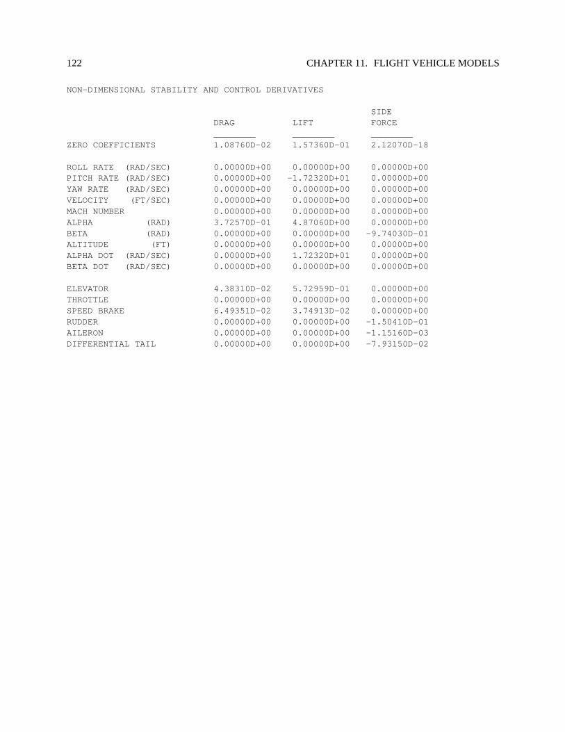
122 CHAPTER 11. FLIGHT VEHICLE MODELS
NON-DIMENSIONAL STABILITY AND CONTROL DERIVATIVES
SIDEDRAG LIFT FORCE________ ________ ________
ZERO COEFFICIENTS 1.08760D-02 1.57360D-01 2.12070D-18
ROLL RATE (RAD/SEC) 0.00000D+00 0.00000D+00 0.00000D+00PITCH RATE (RAD/SEC) 0.00000D+00 -1.72320D+01 0.00000D+00YAW RATE (RAD/SEC) 0.00000D+00 0.00000D+00 0.00000D+00VELOCITY (FT/SEC) 0.00000D+00 0.00000D+00 0.00000D+00MACH NUMBER 0.00000D+00 0.00000D+00 0.00000D+00ALPHA (RAD) 3.72570D-01 4.87060D+00 0.00000D+00BETA (RAD) 0.00000D+00 0.00000D+00 -9.74030D-01ALTITUDE (FT) 0.00000D+00 0.00000D+00 0.00000D+00ALPHA DOT (RAD/SEC) 0.00000D+00 1.72320D+01 0.00000D+00BETA DOT (RAD/SEC) 0.00000D+00 0.00000D+00 0.00000D+00
ELEVATOR 4.38310D-02 5.72959D-01 0.00000D+00THROTTLE 0.00000D+00 0.00000D+00 0.00000D+00SPEED BRAKE 6.49351D-02 3.74913D-02 0.00000D+00RUDDER 0.00000D+00 0.00000D+00 -1.50410D-01AILERON 0.00000D+00 0.00000D+00 -1.15160D-03DIFFERENTIAL TAIL 0.00000D+00 0.00000D+00 -7.93150D-02

11.2. GENERIC F-15 MODEL DATA(SUPERSONIC) 123
NON-DIMENSIONAL STABILITY AND CONTROL DERIVATIVES
ROLLING PITCHING YAWINGMOMENT MOMENT MOMENT________ ________ ________
ZERO COEFFICIENTS 2.77192D-19 4.22040D-02 -1.74198D-19
ROLL RATE (RAD/SEC) -2.00000D-01 0.00000D+00 -3.37210D-02PITCH RATE (RAD/SEC) 0.00000D+00 3.89530D+00 0.00000D+00YAW RATE (RAD/SEC) 1.50990D-01 0.00000D+00 -4.04710D-01VELOCITY (FT/SEC) 3.42955D-17 -1.15312D-10 3.06986D-16MACH NUMBER 3.55618D-14 -1.19570D-07 3.18322D-13ALPHA (RAD) 0.00000D+00 -1.68819D-01 0.00000D+00BETA (RAD) -1.33450D-01 0.00000D+00 1.29960D-01ALTITUDE (FT) 0.00000D+00 0.00000D+00 0.00000D+00ALPHA DOT (RAD/SEC) 0.00000D+00 -1.18870D+01 0.00000D+00BETA DOT (RAD/SEC) 0.00000D+00 0.00000D+00 0.00000D+00
ELEVATOR 0.00000D+00 -6.95279D-01 0.00000D+00THROTTLE 0.00000D+00 0.00000D+00 0.00000D+00SPEED BRAKE 0.00000D+00 -4.17500D-01 0.00000D+00RUDDER -2.38590D-03 0.00000D+00 -6.97630D-02AILERON 2.63560D-02 0.00000D+00 2.19170D-03DIFFERENTIAL TAIL 4.01070D-02 0.00000D+00 3.05310D-02
VEHICLE STATIC MARGIN IS 3.5% MEAN AERODYNAMIC CHORD STABLE