Stability, Flying Qualities and Parameter Estimation of a Twin-Engine CS-23/FAR 23 Certified Light Aircraft

Fabrizio Nicolosi1 and Agostino De Marco2

University of Naples “Federico II”, Naples, Italy

Pierluigi Della Vecchia3

University of Naples “Federico II”, Naples, Italy

This paper presents some results of the flight test campaign conducted on the Tecnam P2006T aircraft, on the occasion of its certification process. This twin-engine propeller airplane is certified under the normal category CS-23 and FAR 23. A prototype of this light aircraft has been tested in flight for a post-design performance optimization and for the assessment of flight qualities. These experiences have led to the application of two winglets to the original wing. The final configuration has been extensively tested for the achievement of CS-23 certification. At the same time the airplane model, through a dedicated set of flight maneuvers, has been characterized by means of parameter estimation studies. The longitudinal and lateral-directional response modes have been assessed and quantified. The aircraft stability derivatives have been estimated from the acquired flight data using the identification technique known as Output Error Method (OEM). Some estimated stability derivatives have been also compared with the corresponding values extracted from leveled flight tests and from wind tunnel tests performed on a scaled model of the aircraft.

Nomenclature ax, ay, az = acceleration of aircraft mass center along the body-fixed x-axis, y-axis, z-axis (m/s2) b = wing span (m) c = reference chord (mean aerodynamic chord) (m) CL, CD , CM = lift coefficient, drag coefficient, moment coefficient Cl, Cn, CY = coefficients of roll moment, yaw moment, side-force Fs = stick control force (N) fn = natural frequency (Hz) Ixx, Iyy, Izz = aircraft moments of inertia (kg m2) lt x , lt y , lt z = coordinates of thrust vector application point in the body-fixed reference frame (m) M = mach number p, q, r = roll, pitch, yaw angular speeds (rad/s) Pa = absolute pressure (N/m2) S = wing area T = thrust (N) or generic oscillation period (s) V = generic speed (m/s) VTAS, VKIAS = true, calibrated airspeeds (m/s) x, y, z = standard body-fixed reference axes, with origin at the center of gravity Xcg = distance of center of gravity from leading edge of mean aerodynamic chord (m)

1 Assistant Professor, Dipartimento di Ingegneria Aerospaziale (DIAS), Via Claudio 21, 80125 Napoli, Italy, AIAA Senior Member. 2 Assistant Professor , Dipartimento di Ingegneria Aerospaziale (DIAS), Via Claudio 21, 80125 Napoli, Italy, AIAA Senior Member. 3 PhD Student, Dipartimento di Ingegneria Aerospaziale (DIAS), Via Claudio 21, 80125 Napoli, Italy.

AIAA Guidance, Navigation, and Control Conference2 - 5 August 2010, Toronto, Ontario Canada

AIAA 2010-7947

Copyright © 2010 by Agostino De Marco, Univ. Naples Federico II, Dept. Aerosp. Eng. Published by the American Institute of Aeronautics and Astronautics, Inc., with permission.

Greek symbols α = angle of attack (rad) β = angle of sideslip (rad) δa, δe, δr = aileron, stabilator, rudder deflection angle (rad) ζ = damping ratio σT = inclination of thrust vector with respect to body-fixed x-axis (rad) Θ = vector of unknown parameters in the aircraft parameter estimation procedure ρ = air density (kg/m3) ψ, θ, φ = airplane heading, elevation, bank angles (rad) ωd = damped pulsation (rad/s) ωn = natural pulsation (rad/s)

I. Introduction HIS paper presents the results of a flight testing research conducted on the P2006T aircraft, an innovative airplane produced by Tecnam (Costruzioni Aeronautiche Tecnam, www.tecnam.com). The purpose of this research is the determination of P2006T stability derivatives and the assessment of its flight qualities through the application of parameter estimation techniques.

The selected airplane is a very light, twin-engine, propeller aircraft, with a maximum take-off weight of 1180 kg. The P2006T design has been presented extensively in other papers.1,2,3 Its main features are summarized in the next section. A large amount of post-design work, and many flight tests have been carried out by the authors during the flight certification of this aircraft under the European category of regulations CS-234 (the airplane is also certified in the FAR 23 category.5 The authors are involved in the flight research activities of the ADAG (Aircraft Design and Aero-flightdynamics Group) at the University of Naples “Federico II”, Department of Aerospace Engineering. The results presented in this work have been achieved after years of research in flight testing focused on flight certification and flight quality assessment of light and ultra-light airplanes. The details of past experiences are found in the cited references.6–8 The flight tests analyzed in the present research took place during the C-S23/FAR 23 certification campaign of the P2006T. Although some flight maneuvers presented here are not strictly required for the certification in these categories, they are necessary for the purpose of aircraft parameter estimation. The reported P2006T flight qualities have been assessed analyzing the response to properly devised command histories. It is seen that the estimated stability derivatives show a good agreement with calculations made in the design phase and with wind tunnel results.

Dynamic characteristics of phugoid, short period, dutch roll modes have been estimated by applying standard methods of analysis to a number of properly excited damped responses. Moreover, the flight data acquired through a dedicated set of performed maneuvers have been used to estimate the aircraft stability derivatives through the well-known ‘maximum likelihood method’ (MLM, see, for example, the book by Jategaonkar9). A Matlab code implementing this method, and based on the classical linearized equations of Flight Dynamics, has been used to construct the aircraft aerodynamic model. In other previous papers written by the authors,7,8 the process of aircraft system identification has been shown and applied to light and ultra-light airplanes and motor-gliders. These flight test experiences have also shown the importance of aircraft system identification to implement a correct and high-fidelity model in a flight simulation environment.

Next section introduces the selected airplane and its main design features. Section III presents the details of the flight test instrumentation used for this work. In section IV the airplane’s stability characteristics and flight qualities are discussed. Estimation of static stability derivatives (both longitudinal and lateral-directional) is presented in sections IV.A and IV.B. The assessment of flight qualities is presented in sections IV.C and IV.D. Finally, in section V the results of aircraft parameter estimation are presented and discussed.

II. The P2006T Aircraft The Tecnam P2006T is a twin-engine, four-seater general aviation airplane with a fully retractable landing gear.

The designer of P2006T is Luigi Pascale, a former professor at the University of Naples, who developed this unique twin-propeller airplane at Tecnam aircraft industries as from 2006. The basic idea of this design consists in having: (i) a high-wing configuration (‘pendular’ stability, high visibility and easy access of passengers and baggage) and (ii) a four-seat aircraft with two light engines taken from the ultra-light world. Thanks to this latter idea, with the

T

P2006T it is the first time that a twin-engine four-seat aircraft has entered in the same market (also with similar price) of single-engine four-seats aircraft, having similar weight and power specifications.

The engine selected by the designer is the Rotax 912S, which is approved for automotive fuel and is FAR33 certified. This engine is of a recent design, and is the result of all the latest technologies developed for the automotive market. With respect to the standard General Aviation engines, the Rotax 912S has a reduced frontal area, a better weight-to-power ratio, lower specific fuel consumption, lower propeller rpm (i.e. higher efficiency and lower acoustic emissions), more stable engine head temperatures (due to liquid cooling).

From Table 1 to Table 5 we have reported all the main geometric characteristics, weights and cg range, propulsion data, and performances of the certified airplane. The three-view drawing of P2006T aircraft is shown in Fig. 1, and a picture of the airplane during flight tests is presented in Fig. . The horizontal empennage of this airplane is a stabilator, i.e. an ‘all moving tail’ whose deflection is called here δe or δs interchangeably.

Table 3. P2006T Aircraft Propulsion Characteristics

Engine Model Rotax 912S

Take-off Power 100 hp (73 kW)

Maximum Continuous Power 92.4 hb (69 kW)

Propeller (2 Blades, Constant Speed, Full Feathering) MTV-21-A-C-F/CF178-05

Table 2. P2006T Aircraft Weights, Loading and Inertia

Maximum Take-off Weight 2601 lb (1180 kg)

Standard Equipped Weight 1675 lb (760 kg)

Standard Useful Load 926 lb (420 kg)

Aircraft Mom. of Inertia Ixx , Iyy , Izz 1193, 1421, 2162 (slug ft2) (1617, 1927, 2931 kg m2)

Limit Load Factors +3.8 g / −1.9 g

Table 1. P2006T Aircraft Geometric Characteristics.

Wing Span 37.40 ft (11.4 m) Fuselage Height 9.35 ft (2.85 m)

Wing Area 159.31 ft2 (14.8 m2) Cabin Width 48.03 in (1.22 m)

Fuselage Length 28.50 ft (8.7 m) Cabin Length (with bagg.) 11 ft (3.35 m)

Figure 1. Three view drawing of P2006T Aircraft (Courtesy by Tecnam)

Table 5. Selected cg range for flight tests.

Max Forward Max Aft

Xcg / c 16.5% 31%

Table 4. P2006T Performances

Max Speed at Sea Level 155 kts

Cruise Speed (75%, 7000 ft) 145 kts

Cruise speed (65%, 9000 ft) 135 kts

Stall Speed Flap Down 47 kts

VA (Maneuvering Speed) 116 kts

VNE (Never Exceed Speed) 168 kts

Climb Rate, S.L. 1260 ft/min

Climb rate, S.L., One Engine Inoperative (OEI) 300 ft/min

Service Ceiling (Twin Engine) 15000 ft

Single-Engine Ceiling 7000 ft

Take-off Distance 1476 ft (450 m)

Take-off Run 771 ft (235 m)

Landing Distance 1050 ft (320 m)

Landing Run 623 ft (190 m)

The configuration of the selected airplane has been extensively tested in the wind tunnel. Pictures of a scaled model of P2006T in the low-speed wind tunnel of the University of Naples “Federico II” are presented in Fig. 3. A selection of aerodynamic curves resulting from wind tunnel experiments are reported in Fig. 4 and Fig. 5 (see also Fig. 25). The aerodynamic coefficients are measured for a fixed transition (transition strips applied on wings, nacelles and fuselage, see Fig. 3) and a reference Reynolds number equal to 0.6×106 (see Ref. 2 and 3).

III. The Flight Test Instrumentation Flight data have been acquired through a light, fast and reliable flight test instrumentation. The choice of a

particular test equipment depends on the type of required flight test campaign, and on the desired accuracy. The importance of selecting reliable and accurate test instruments emerged in a number of past experiences on similar airplanes.6,7,8 The instrumentation used for the present research (both sensors and acquisition system) is the evolution

Figure 3 Scaled model of P2006T in the low-speed wind tunnel of the University of Naples “Federico II”.

The configuration has been investigated with and without nacelles. All tests have been performed at fixed transition, i.e. by using transition strips on wing, nacelles and fuselage, and with a reference

Reynolds number of 0.6×106 (see Ref. 2, 3).

Figure 2. P2006T during a flight test (Courtesy by Tecnam)

of the one utilized by the authors for all flight tests on ultra-light airplanes since 1998. The present system represents a very good compromise between costs and performances.

The flight data acquisition system consists in a central unit, named CSYS (Central SYStem), which is shown in Fig. 6. It includes an airborne computer equipped with dedicated cards for the conditioning and control of signals. All signals come from a set of flight sensors appropriately connected to the central unit.

The CSYS is a transportable and complete data acquisition system, designed for the gathering of flight data, their storage on magnetic support, and their remote transmission in real time to operators on ground. It integrates a differential GPS and is easily interfaced with an AHRS-400 inertial platform (see also Fig. 6), which is placed close to aircraft center of gravity. When equipped with an external radio modem, the system is able to transmit the data in real time to a remote ground station.

The CSYS includes a National Instruments card, which is the main building block of the data acquisition hardware. Multiplexing, conditioning and signal control technologies are embedded into the CSYS case. The system is able to acquire 32 analogue channels and 6 digital channels. It has 4 analogue output ports, 4 USB ports and other typical PC connections.

During the tests the aircraft has been equipped with sensors for the acquisition and measurement of flight data. Pressure transducers have been installed to measure the anemometric speed and altitude. For these sensors we have assessed an accuracy of about 0.5 kts on flight speed and of 3 feet on altitude. A special sensor (mini air-data boom) for the measurement of angle of attack and angle of sideslip, was mounted on the nose of the aircraft (see Fig. 7).

A particular care has been taken in mounting a load cell on the control stick in order to measure the piloting effort (Fig. 8). A set of potentiometers has been installed on the aircraft control lines to measure the deflection of control surfaces (Fig. 9).

A very accurate inertial measurement unit (XBow AHRS 400) has been used to measure angles, accelerations and angular rates. Almost all flight tests have been performed with a 10 Hz sampling rate. The system is also equipped with a dual frequency GPS for position and ground speed measurement. The GPS has been acquired simultaneously to other flight data and with a sample rate of 10 Hz.

Figure 4. Wind tunnel longitudinal data on a scaled model of P2006T.

Pitching moment coefficient, measured for a fixed transition on wings, nacelles and fuselage and a reference Reynolds number of 0.6×106, at different stabilator deflection angles δs (see Ref. [2], [3]).

Note the negative value of the CM 0 , i.e. of CM at α=0 deg and δs=0 deg.

Figure 5. Wind tunnel lateral-directional data on a scaled model of P2006T.

Side-force (top), roll moment (middle), yaw moment (bottom) coefficients, measured for a fixed transition on wings, nacelles and fuselage and a reference Reynolds number of 0.6×106, at different rudder deflection angles δr (see Ref. 2, 3).

IV. Stability and Flight Qualities The analysis of aircraft stability and flight qualities has been carried out according to the regulation

requirements. For these tests, load cells have been used to measure the stick forces. The results discussed below show a stable behavior of the airplane.

A. Static Longitudinal Stability The static longitudinal stability test for this type of airplane must demonstrate that—starting from a trimmed

flight condition—when the pilot applies a pulling or pushing force to the longitudinal control, and then releases the stick slowly, the airplane finally returns in a trimmed condition, with a tolerance margin of 10% on the initial equilibrium speed. Besides, according to CS-23, it must be demonstrated that “a pull must be required to obtain and maintain speeds below the specified trim speed, and that a push is required to obtain and maintain speeds above the specified trim speed.” Figure 10 shows that these requirements are met.

The aircraft stick-fixed static stability margin has also been measured. Through establishing several level flight conditions, the stabilator deflections and flight speeds have been acquired at different center of gravity positions. Figure 11a shows the obtained results. The analysis of Fig. 11a, according to the technique suggested by Kimberlin10 allows the measurement of the stick-fixed neutral point at different flight speeds, as shown in Fig. 11b. The neutral point position in cruise condition (CL = 0.50) is located at about the 43% of the reference chord and is in good agreement with wind tunnel measurements.2 For the other two conditions examined (i.e. at different values of level flight lift coefficient, 0.90 and 0.25), the scattered and lacking data do not seem to lead to reliable results. However, the higher slope dδs/dα (higher static margin) at higher lift coefficients is clearly shown in Fig. 11a. This is the well-

Figure 6 . Main Box and Inertial Platform.

Figure 7. Pitot probe with α- and β-flags.

Figure 8. Load cells for stick force measurements.

Figure 9. Position transducer – Aileron control

known ‘pendular stability’ effect, also observed during wind tunnel tests, and is due to the low position of the center of gravity with respect to the wing.

B. Static Lateral-Directional Stability A significant amount of information concerning the aircraft lateral-directional stability characteristics have been

obtained by measuring the deflection of control surfaces, the piloting efforts, the angle of sideslip and the angle of bank, while keeping the airplane in steady yawed flight. An example of such a test is represented by Fig. 12.

(a) (b)

Figure 11. (a) Required stabilator deflections for level flight, for maximum forward and maximum aft positions of aircraft center of gravity.

(b) Stick-fixed Neutral point estimation at different level flight speeds. It is evident that the airplane, in the whole range of operating speeds, is always trimmed with a negative

stabilator deflection (trailing edge up).

Figure 10. Static longitudinal stability test (time histories).

When a trimmed condition is established, the pilot applies a gradual pulling to the longitudinal control and then releases the stick slowly.

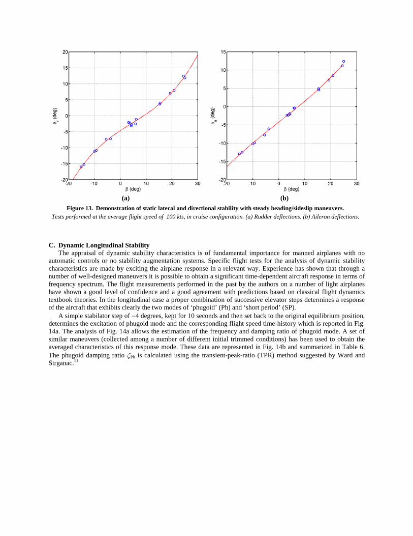
Figure 13 shows that the airplane is statically stable both laterally and directionally. Figure 13a reports the required rudder deflections to keep a given sideslip angle (the asymmetry of the curve is due to the effect of non counter-rotating propellers). Figure 13b shows that, for positive sideslip angles, the pilot needs to compensate with the right aileron downward deflections, to avoid the excessive wing bank.

Figure 12. Demonstration of static lateral and directional stability with steady heading/sideslip maneuvers.

Average flight speed of 100 kts, in cruise configuration. Time histories showing that the airplane is kept for successive time intervals

of approximately ten seconds at different fixed sideslip angles.

C. Dynamic Longitudinal Stability The appraisal of dynamic stability characteristics is of fundamental importance for manned airplanes with no

automatic controls or no stability augmentation systems. Specific flight tests for the analysis of dynamic stability characteristics are made by exciting the airplane response in a relevant way. Experience has shown that through a number of well-designed maneuvers it is possible to obtain a significant time-dependent aircraft response in terms of frequency spectrum. The flight measurements performed in the past by the authors on a number of light airplanes have shown a good level of confidence and a good agreement with predictions based on classical flight dynamics textbook theories. In the longitudinal case a proper combination of successive elevator steps determines a response of the aircraft that exhibits clearly the two modes of ‘phugoid’ (Ph) and ‘short period’ (SP).

A simple stabilator step of −4 degrees, kept for 10 seconds and then set back to the original equilibrium position, determines the excitation of phugoid mode and the corresponding flight speed time-history which is reported in Fig. 14a. The analysis of Fig. 14a allows the estimation of the frequency and damping ratio of phugoid mode. A set of similar maneuvers (collected among a number of different initial trimmed conditions) has been used to obtain the averaged characteristics of this response mode. These data are represented in Fig. 14b and summarized in Table 6. The phugoid damping ratio ζPh is calculated using the transient-peak-ratio (TPR) method suggested by Ward and Strganac.11

(a) (b)

Figure 13. Demonstration of static lateral and directional stability with steady heading/sideslip maneuvers. Tests performed at the average flight speed of 100 kts, in cruise configuration. (a) Rudder deflections. (b) Aileron deflections.

It has to be observed that CS-23 and FAR 23 regulations do not require a specific quantitative evaluation of the

phugoid response. They simply state that “any long period oscillation of the flight path (phugoid) must not be so unstable as to cause an unacceptable increase in pilot workload.” In all flight tests the pilot has reported a stable phugoid behavior of the selected airplane, without any additional workload required to stabilize the speed oscillations.

The airplane’s fast dynamics has been investigated analyzing the time responses of several ‘3211-type’ longitudinal tests (see later in section V.A). An example of angle-of-attack time-history is presented in Fig. 15a, where the symbol notation from Kimberlin’s book10 has been used. From these kind of flight responses we have estimated the averaged parameters of the short period mode. The original raw data have been filtered in order to get a set of smooth curves, such as that of Fig. 15a. The unfiltered data are disturbed by the elastic deformations of the boom, the α-flag inertia, and the atmospheric turbulence. However, the filtered curves are representative of a typical damped angle-of-attack response of a short period excitation. The damping characteristics, being the short period mode heavily damped, have been obtained with the ‘maximum-slope’ (MS) method (Fig. 15b with values from Fig. 15a), suggested both by Kimberlin10 and Ward and Strganac.11 The results are represented in Fig. 16b and summarized in Table 7. For the purpose of comparison with the well known ‘thumb print’ criterion curves, which are valid for different categories of airplanes, the collocation of the P2006T in the (ζ,ωn)-plane is shown in Fig. 16a.

Table 6. Characteristics of phugoid motion.

Damped period, TPh 27 s

Damping ratio, ζPh 0.09

Damped pulsation, ωd,Ph 0.233 rad/s

Natural pulsation, ωn,Ph 0.234 rad/s

(a) (b)

Figure 14. Typical phugoid response and characteristic roots. (a) Speed variation, with respect to a trimmed condition in level flight at 110 kts. Obtained with a step stabilator

deflection of -4 degrees, kept for 10 seconds. (b) Averaged damped oscillation parameters in the imaginary plane, extracted over a number of time histories similar to curve (a).

(a) (b) Figure 16. Typical short period response and characteristic roots.

(a) Placement of P2006T into the ‘thumb print’ plot. (b) Averaged damped oscillation parameters in the imaginary plane, extracted from a number of similar time histories (excited by ‘3211-type’ longitudinal command input).

(a) (b) Figure 15. Typical short period response and maximum-slope method.

(a) Angle-of-attack the time history is a response to a ‘3-2-1-1-type’ stabilator input. The notation is taken from Kimberlin’s book (Ref. 10).

(b) Plot used to estimate the short period natural pulsation with the maximum-slope method (see Ref. 10, 11).

Table 7 reports the value of the short period time constant τSP, computed as:14

τSP = −1 / Zα = m / ( Q0 S CLα ) (1)

where the dynamic pressure Q0 is referred to the initial trimmed conditions at VTAS = 113 kts (58 m/s) and aircraft mass of 1140 kg. The lift curve slope in equation (1) is the value given as a result of the aircraft parameter estimation technique discussed later in section V.A. This leads to the computation of the following value of the control anticipation parameter:

CAP = ωn,SP2 / nα ≈ mg ωn,SP

2 / ( Q0 S CLα ) = 1.009 (2)

Corresponding to a value nα = 11.5. The above value of CAP, given the calculated damping ratio ζSP and natural pulsation ωn,SP presented in Table 7, collocates the short period flight quality of the selected airplane well within the Level 1 range (Class I-B, see Ref. 14 and 17).

D. Dynamic Lateral-Directional Stability The typical maneuver used for the excitation of aircraft ‘dutch roll’ mode is a multi-step rudder deflection. An

example of such a test is shown in Fig. 17. The damping of lateral-directional oscillating responses is typically less than the damping of the fast longitudinal ones, such as the short period. Moreover, the roll and yaw motions are always coupled and this adds difficulties to the flight data analysis work.

Figure 17. Example of dutch roll excitement with multiple pedal doublets.

For the sake of clarity, in the heading angle time history, the ψ variable is not represented in the standard range (0,2π) to avoid discontinuities.

Table 7. Characteristics of Short-Period motion.

Time constant, τSP 0.0088 s

Damping ratio, ζSP 0.40

Damped pulsation, ωd,SP 3.125 rad/s

Damped period, TSP 1.84 s

Natural pulsation, ωn,SP 3.410 rad/s

Natural frequency, fn,SP=ωn,SP / 2π 0.54 (cps)

The quality of dutch roll damping, when excited by a multi-step pedal input is easily seen by inspecting the time histories of Fig. 17. The test pilot has reported the perception of good damping behavior of the P2006T aircraft in these kind of maneuvers.

Among the possible methods of excitation, specific to the dutch roll response, the most effective test has consisted in asking the pilot for a simple pedal doublet. This test determines the minimum amount of coupling between roll and yaw oscillations. However, if the pilot input is not quite symmetric, it is very easy to excite the roll mode and/or the spiral mode and make data analysis difficult. The time histories of Fig. 18 are obtained with a simple pedal doublet. This example clearly exhibits the typical dutch roll mode response. This figure shows a dutch roll period of the order of magnitude of 3 seconds. This is confirmed by other similar tests at different initial speeds and altitudes.

An evaluation of the dutch roll damping characteristics from flight measured oscillating sideslip response is shown in Fig. 19. The transient-peak-ratio method proposed by Ward and Strganac11 applied to the β curve of Fig. 19 value leads to an average TPR of 0.43 and a corresponding damping ratio ζDR = 0.26. The measured average damped period of 3.25 s and the resulting pulsations ωd,DR and ωn,DR are reported in Table 8. The calculated time factor ζDRωn,DR = 0.52 is in very good agreement with the average time factor (0.50) of the exponential enveloping curves (dashed lines) shown also in Fig. 19.

Figure 18. Example of Dutch-Roll response.

For the sake of clarity, in the heading angle time history, the ψ variable is not represented in the standard range (0,2π) to avoid discontinuities.

These flight results confirm the approximate values that can be obtained through the method suggested by Kimberlin10 and Langdon12 and based on the knowledge of aircraft directional stability derivative Cnβ. This approximate method suggests the use of the following formula:

zzn I

bSPCM2

aDRn,

γω β≈

(3)

for the estimation of dutch roll natural pulsation, where M is the flight Mach number, γ is the air heat capacity ratio, Pa the absolute pressure, Izz the moment of inertia with respect to the z-body axis. Using a value of Cnβ = 0.52 rad−1, extracted from wind tunnel tests performed on a scaled model of P2006T, and M = 0.16, Pa = 97800 N/m2 (flight speed and altitude of the considered test), and Izz = 2931 kg m2 (see also Table 2), S = 14.8 m2, b = 11.4 m, the above formula leads to a value of ωn,DR = 2.36 rad/s. This value is very near to the value (2.00) derived from flight data (Table 8). The approximate damping ratio is estimated by assuming (see Ref. 10) that Yβ = Nr. This leads to the approximate formula:

zznrn IC

bSCβ

ρζ8

3

DR =

(4)

Table 8. Characteristics of Dutch-Roll motion.

Damped period, TDR 3.25 s

Damping ratio, ζDR 0.26

Damped pulsation, ωd,DR 1.93 rad/s

Natural pulsation, ωn,DR 2.00 rad/s

Time factor, ηDR =ζDRωn,DR 0.52 rad/s

Figure 19. Dutch-Roll response to a simple pedal doublet excitation.

Initial Leveled flight at speed 110 kts (Mach number 0.16), altitude 1000 ft.

where ρ is the air density and Cnr the aircraft yaw damping derivative. We can assume a value Cnr = −0.084 rad−1 based on the semi-empirical formula suggested by Roskam,13 which depends mainly on the contribution (CYβ,)V, due to the vertical tail, to the total CYβ. The vertical tail contribution to side-force coefficient derivative has been extracted from wind tunnel test data and is equal to CYβ,V = −0.084 rad−1. Finally, the above formula applied to the P2006T gives a ζDR = 0.38. This value is slightly higher than the flight measured value given in Table 8, probably due to the fact that wind tunnel data are valid for power-off conditions and lower Reynolds numbers. The same consideration applies to the discrepancy of the calculated pulsation with respect to the flight measured value.

In Fig. 20 we have reported an example of roll mode test. Typically, these responses settle down completely in about 3 seconds, which is a typical behavior of dutch roll mode. This confirms that the roll mode part of such a response is very difficult to quantify because its time constant is too short be observed manually. In this respect it has been accepted the good feedback of the pilot about the rolling behavior of this aircraft.

V. Aircraft Parameter Estimation It is well known that the stability derivatives of airplanes can be estimated through the analysis of flight test data.

This process goes under the name of ‘aircraft system identification’ or aircraft ‘parameter estimation’. The key element of all parameter estimation methods is a computer program that seeks to replicate recorded flight test time histories of output variables by varying a given set Θ of coefficients in a linearized model of the aircraft. In this process also pilot inputs are measured and used to calculate the unknown coefficients Θi in the aircraft equations of motion. Most of the elements of Θ are the desired values of aircraft stability derivatives referred to a given flight condition. A detailed discussion of the available parameter estimation methods is found in the advanced text by Jategaonkar.9 The selected technique of flight data analysis for the tests on P2006T aircraft is the one known as ‘Output Error Method’ (OEM). The application of the OEM and the process of estimating stability derivatives are summarized here. In Fig. 21 is presented a block schematic of this parameter estimation technique.

The mathematical model of aircraft flight dynamics is derived from the rigid-body equations of motion projected onto the standard body-fixed reference frame, coupled with a set of auxiliary kinematic equations. The linearized equations are decoupled into longitudinal and lateral-directional sets.

Figure 20. Roll response to aileron singlet.

Initial Leveled flight at speed 110 kts (Mach number 0.16), altitude 1000 ft. The bank angle change of such a maneuver is about 40 degrees.

In the longitudinal case the linearized equations are written in the following form:

)cossin(

)sin()cos(

)cos()sin(

TztTxtyy

Myy

TL

TD

llITC

IcSQq

q

mVT

VgqC

VmSQ

mTgC

mSQV

σσ

θ

σαθαα

σαθα

++=

=

+−−++=

++−+=

(5)

Regarding the above system as the set of aircraft state equations, the corresponding set of longitudinal observation equations is the following:

TZz

TXx

TztTxtyy

Myy

mTC

mQSa

mTC

mSQa

llITC

IcSQq

qqVV

σ

σ

σσ

θθαα

sin

cos

)cossin(

,,,

+=

+=

++=

====

m

m

m

mmmm

(6)

where the subscript ‘m’ denotes the measured variables. In the above equations the body-force coefficients CX and CZ are given by:

αααα sincos,cossin DLZDLX CCCCCC −−=−= (7)

The linearized longitudinal aircraft aerodynamic model is expressed by the coefficients:

s0

000 s2δααα δααα MqMMMMLLLDDD C

VcQCCCCCCCCCC +++=+=+= ,, (8)

The above equations (7)-(8), having assumed (V, α, θ, q) as state variables and (δs, T) as input variables, introduces the unknown parameters:

Θ lon = [CD0, CDα, CL0, CLα, CM0, CMα, CM q, CM δs] (9)

forming the unknown vector Θ lon for the longitudinal dynamics. Each maneuver considered in the present work starts from a trimmed state. In these conditions, knowing the equilibrium airspeed, the thrust T has been calculated

Figure 21. Block schematic of Output Error Method (OEM)

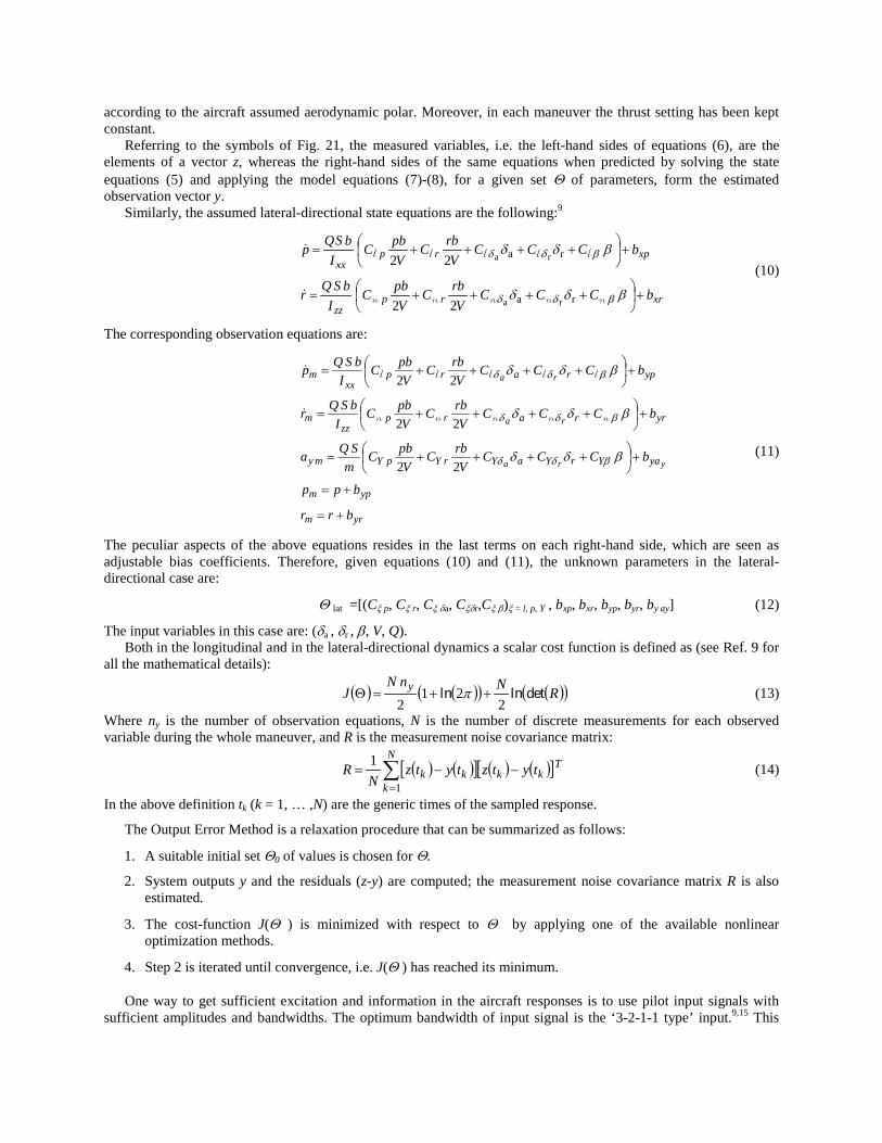
according to the aircraft assumed aerodynamic polar. Moreover, in each maneuver the thrust setting has been kept constant. Referring to the symbols of Fig. 21, the measured variables, i.e. the left-hand sides of equations (6), are the elements of a vector z, whereas the right-hand sides of the same equations when predicted by solving the state equations (5) and applying the model equations (7)-(8), for a given set Θ of parameters, form the estimated observation vector y.

Similarly, the assumed lateral-directional state equations are the following:9

xrrpzz

xprpxx

bCCCV

rbCV

pbCI

bSQr

bCCCV

rbCV

pbCI

bSQp

+

++++=

+

++++=

βδδ

βδδ

βδδ

βδδ

nnnnn

lllll

ra

ra

ra

ra

22

22

(10)

The corresponding observation equations are:

yrm

ypm

yaYrYaYrYpYmy

yrrarpzz

m

yprarpxx

m

brr

bpp

bCCCV

rbCV

pbCm

SQa

bCCCV

rbCV

pbCI

bSQr

bCCCV

rbCV

pbCI

bSQp

yra

ra

ra

+=

+=

+

++++=

+

++++=

+

++++=

βδδ

βδδ

βδδ

βδδ

βδδ

βδδ

22

22

22

nnnnn

lllll

(11)

The peculiar aspects of the above equations resides in the last terms on each right-hand side, which are seen as adjustable bias coefficients. Therefore, given equations (10) and (11), the unknown parameters in the lateral-directional case are:

Θ lat =[(Cξ p, Cξ r, Cξ δa, Cξδr,Cξ β)ξ = l, p, Y , bxp, bxr, byp, byr, by ay] (12)

The input variables in this case are: (δa , δr , β, V, Q). Both in the longitudinal and in the lateral-directional dynamics a scalar cost function is defined as (see Ref. 9 for

all the mathematical details):

( ) ( )( ) ( )( )RNnNJ y detlnln

221

2++=Θ π (13)

Where ny is the number of observation equations, N is the number of discrete measurements for each observed variable during the whole maneuver, and R is the measurement noise covariance matrix:

( ) ( )[ ] ( ) ( )[ ]∑=

−−=N

k

Tkkkk tytztytz

NR

1

1 (14)

In the above definition tk (k = 1, … ,N) are the generic times of the sampled response.

The Output Error Method is a relaxation procedure that can be summarized as follows:

1. A suitable initial set Θ0 of values is chosen for Θ.

2. System outputs y and the residuals (z-y) are computed; the measurement noise covariance matrix R is also estimated.

3. The cost-function J(Θ ) is minimized with respect to Θ by applying one of the available nonlinear optimization methods.

4. Step 2 is iterated until convergence, i.e. J(Θ ) has reached its minimum.

One way to get sufficient excitation and information in the aircraft responses is to use pilot input signals with sufficient amplitudes and bandwidths. The optimum bandwidth of input signal is the ‘3-2-1-1 type’ input.9,15 This

kind of input is reported, for instance, in Fig. 22 (‘Maneuver 3’) for the longitudinal control. It is a sequence of four steps of opposite signs. The first three steps have, respectively, a duration of 3, 2 and 1 times the duration of the last step. Since parameter estimation is based on small perturbation analysis, the amplitude of pilot input is to be chosen to restrict the aircraft response within the linear range.

The process that has been used for the estimation of the aircraft parameters is articulated as follows: (i) choice of the model equations capable to describe the motion of the airplane (both in the longitudinal and lateral-directional case), (ii) selection of the right sequence of maneuvers and measured responses as inputs to the estimation algorithm, (iii) determination of initial parameters based on semi-empirical analyses and wind tunnel test data. Obviously, the model requires the knowledge of aircraft mass, inertia (see Table 2) and propulsive thrust (estimated through the flight measured aircraft flight polar) in the considered flight condition.

The results of the application of this process to the longitudinal and lateral-directional motions of the P2006T aircraft are reported in the following subsections. All the tests have been performed starting from level flight and with the following initial conditions: flight speed of VKIAS = 110 kts (57 m/s), a mass of 1140 kg (slightly lower than MWTO condition), Xcg / c = 19%.

A. Identification of Longitudinal Characteristics An example of measured longitudinal input sequence used by the system identification software is reported in

Fig. 22. This figure demonstrates how a number of separate input laws are simply lined-up in one single stream of data and given as one sequence to the relaxation algorithm, as if it was a unique input. Actually, the maneuvers have been physically performed and acquired in separate tests. This explains why some discontinuities may appear in flight parameters (e.g. between maneuver 2 and 3, see Fig. 22 and Fig. 23). Such a sequence of multiple maneuvers seems to be the preferred way to obtain a reliable estimate of the aircraft aerodynamic model because it is able to excite the broadest variety of longitudinal motions, with a fairly large frequency spectrum. The set of aerodynamic derivatives obtained at the end of the convergence process leads to a simulated output very close to the flight measured data. This is clearly observed by inspecting the time histories of Fig. 23. The converged set Θ of parameters is used to check the quality of the estimation procedure. The aircraft model based on Θ is used to evaluate the difference between the simulated output and a flight response which has not been considered previously in the relaxation procedure. For instance, in Fig. 24 the simulated output due to a longitudinal stabilator doublet [δe(t) not included in the sequence of Fig. 22] is compared with the flight measured data. It is seen that also positive and negative peaks of measured responses (flight speed and vertical acceleration) are in good agreement with the estimated ones.

In Table 9 the complete set of estimated aerodynamic longitudinal derivatives (aircraft aerodynamic model) is presented. In the same table we have reported also the derivatives based on wind tunnel results. The damping derivative Cm q calculated with a semi-empirical formula13 is also reported in Table 9. Considering that the wind tunnel test data do not take into account the effect of propellers, and that their reference Reynolds number is lower than the flight Reynolds number, the agreement between wind tunnel and parameter estimation can be considered quite good, especially for the pitching moment coefficient derivatives (i.e. Cm α and Cm δe ). The estimated lift coefficient slope CL α (see Table 9) is slightly lower than the one observed during wind tunnel tests. This minor discrepancy is probably due to the effect of nacelles in presence of running propellers, which was not replicated in wind tunnel model.

Figure 23. Example of Parameter Estimation Results for the Longitudinal Case.

The output of the parameter estimation iterative algorithm is the set of longitudinal stability derivatives [see Eq. (7)], which are the coefficients of the linearized aircraft equations of motion. The ‘Estimated’ curves are obtained by solving

the equations with the converged values of the coefficients.

Figure 22. Example of multiple longitudinal inputs to the parameter estimation algorithm.

The input laws are simply lined-up in one single stream of data and provided to the algorithm as if it was a unique input. Actually, the maneuvers were physically performed and acquired in separate tests.

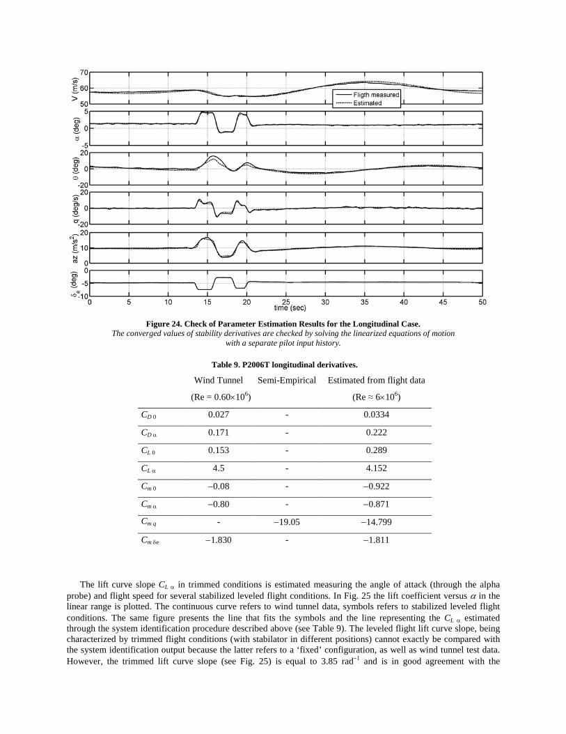
The lift curve slope CL α in trimmed conditions is estimated measuring the angle of attack (through the alpha probe) and flight speed for several stabilized leveled flight conditions. In Fig. 25 the lift coefficient versus α in the linear range is plotted. The continuous curve refers to wind tunnel data, symbols refers to stabilized leveled flight conditions. The same figure presents the line that fits the symbols and the line representing the CL α estimated through the system identification procedure described above (see Table 9). The leveled flight lift curve slope, being characterized by trimmed flight conditions (with stabilator in different positions) cannot exactly be compared with the system identification output because the latter refers to a ‘fixed’ configuration, as well as wind tunnel test data. However, the trimmed lift curve slope (see Fig. 25) is equal to 3.85 rad−1 and is in good agreement with the

Table 9. P2006T longitudinal derivatives.

Wind Tunnel Semi-Empirical Estimated from flight data

(Re = 0.60×106) (Re ≈ 6×106)

CD 0 0.027 - 0.0334

CD α

0.171 - 0.222

CL 0 0.153 - 0.289

CL α

4.5 - 4.152

Cm 0 −0.08 - −0.922

Cm α

−0.80 - −0.871

Cm q

- −19.05 −14.799

Cm δe

−1.830 - −1.811

Figure 24. Check of Parameter Estimation Results for the Longitudinal Case.

The converged values of stability derivatives are checked by solving the linearized equations of motion with a separate pilot input history.

estimated slope reported in Table 9. The wind tunnel data, as already mentioned, are relative to a power-off condition (wind tunnel test model was only with nacelles) and at a significant lower Reynolds number (wind tunnel tests were performed at Re = 0.6 ×106 based on model’s mean aerodynamic chord while flight data refers to a flight Reynolds number of about 6×106, as also reported in Table 9).

B. Identification of Lateral-Directional Characteristics As for the longitudinal case, the OEM has been applied to the linearized lateral-directional model given by

equations (10) and (11) and taken from Ref. 9. The unknowns in this case are given by the definition (10). An example of sequence of measured lateral-directional inputs is reported in Fig. 26. As can be observed, both aileron (continuous line) and rudder (dotted line) inputs have been used to excite completely the lateral-directional motions of the aircraft.

Figure 26. Example of multiple lateral-directional inputs to the parameter estimation algorithm.

Figure 25. The equilibrium CL versus α from flight tests at different speeds. The slope CLα is compared with parameter estimation wind tunnel results.

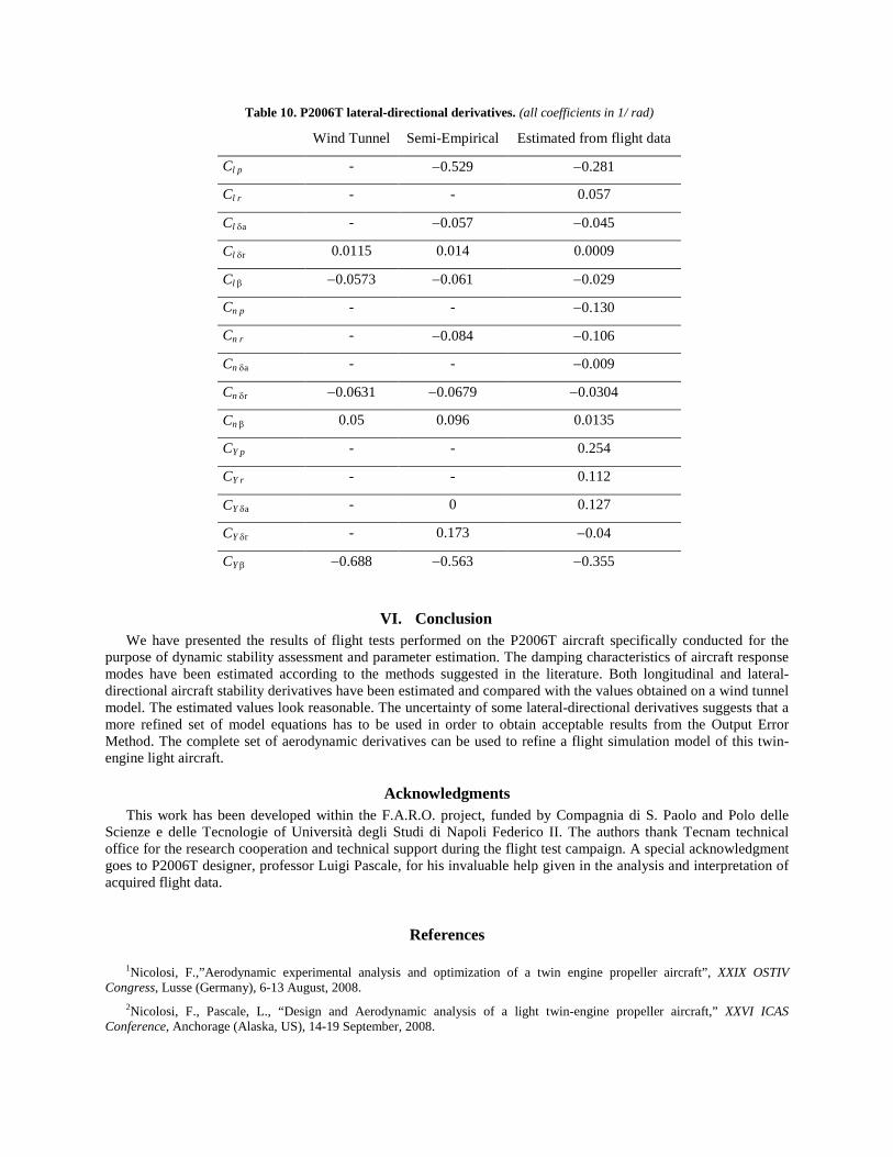
In Fig. 27 is presented an example of comparison between simulated output, based on a converged set of parameters, and flight measured responses. The agreement between simulated (estimated model) and flight data seems acceptable. However, the simplicity of the particular model equations considered here permits the discrepancies observed in the time history of lateral acceleration ay. In Table 10 the estimated lateral-directional aerodynamic derivatives are reported. The same table also presents some values obtained from wind tunnel tests (with the same considerations on Reynolds and power effects described above) and with semi-empirical formulae (as suggested by Ref. 13). Good agreement between semi-empirical estimation and parameter estimation is observed for roll control derivatives Cl δa and Cl δr and yaw-damping derivative Cn r. Although the simulated output is a good match of measured data (see Table 10 and Fig. 27), the other derivatives (i.e. Cn β and Cl β) do not seem to be well estimated and significant discrepancies are observed with semi-empirical and wind tunnel data. To improve accuracy in the estimation of these coefficients, the model of equations to be used has to be improved. In fact, also the equation representing the equilibrium along y-axis (equation for lateral acceleration ay ) has to be added in the model (3 equations instead of two equations) to improve the accuracy in all derivatives.

Figure 27. Example of parameter estimation results.

The dashed curves refer to the simulated time histories obtained with the lateral-directional stability derivatives converged values.

VI. Conclusion We have presented the results of flight tests performed on the P2006T aircraft specifically conducted for the

purpose of dynamic stability assessment and parameter estimation. The damping characteristics of aircraft response modes have been estimated according to the methods suggested in the literature. Both longitudinal and lateral-directional aircraft stability derivatives have been estimated and compared with the values obtained on a wind tunnel model. The estimated values look reasonable. The uncertainty of some lateral-directional derivatives suggests that a more refined set of model equations has to be used in order to obtain acceptable results from the Output Error Method. The complete set of aerodynamic derivatives can be used to refine a flight simulation model of this twin-engine light aircraft.

Acknowledgments This work has been developed within the F.A.R.O. project, funded by Compagnia di S. Paolo and Polo delle

Scienze e delle Tecnologie of Università degli Studi di Napoli Federico II. The authors thank Tecnam technical office for the research cooperation and technical support during the flight test campaign. A special acknowledgment goes to P2006T designer, professor Luigi Pascale, for his invaluable help given in the analysis and interpretation of acquired flight data.

References 1Nicolosi, F.,”Aerodynamic experimental analysis and optimization of a twin engine propeller aircraft”, XXIX OSTIV

Congress, Lusse (Germany), 6-13 August, 2008. 2Nicolosi, F., Pascale, L., “Design and Aerodynamic analysis of a light twin-engine propeller aircraft,” XXVI ICAS

Conference, Anchorage (Alaska, US), 14-19 September, 2008.

Table 10. P2006T lateral-directional derivatives. (all coefficients in 1/ rad)

Wind Tunnel Semi-Empirical Estimated from flight data

Cl p - −0.529 −0.281

Cl r - - 0.057

Cl δa - −0.057 −0.045

Cl δr 0.0115 0.014 0.0009

Cl β −0.0573 −0.061 −0.029

Cn p - - −0.130

Cn r - −0.084 −0.106

Cn δa - - −0.009

Cn δr −0.0631 −0.0679 −0.0304

Cn β 0.05 0.096 0.0135

CY p - - 0.254

CY r - - 0.112

CY δa - 0 0.127

CY δr - 0.173 −0.04

CY β −0.688 −0.563 −0.355

3Pascale, L, Nicolosi, F., “Design of a twin engine propeller aircraft; aerodynamic investigation on fuselage and nacelle effects,” Aerotecnica Missili e Spazio, Vol. 87 , No. 3/2008, Luglio-Settembre 2008, pp. 99-114.

4“Certification Specifications for Normal, Utility, Aerobatic and Commuter Category Airplanes,” CS-23, EASA, 2003. 5FAA Advisory Circular No. 23-8A, “Flight Test Guide for Certification of Part 23 Airplanes,” U.S. Dep. Of Transportation,

FAA, Washington, D.C., Feb. 1989. 6Iscold, P. H. A. de O., Ribeiro, R. P., Pinto, R. L. U. de F., Resende, L. S., Coiro, D. P., Nicolosi, F. and Genito, N., “Light

Aircraft Instrumentation to Determine Performance, Stability and Control Characteristics in Flight Tests,” SAE BRASIL Congress, 2004, SAE Technical Papers Series, ISSN 0148-7191.

7Coiro, D. P., Nicolosi, F., De Marco, A., Genito, N., “Dynamic Behavior and Performances Determination of DG400 Sailplane through Flight Tests,” Technical Soaring, Vol. 27, Num. 1 and 2, January-April 2003; ISSN 0744-8966

8Coiro, D. P., Nicolosi, F., De Marco, A., Familio, R., “Flight Test on Ultralight Motorglider, Aerodynamic Model Estimation and Use in a 6DOF Flight Simulator,” Aerotecnica , Missili e Spazio, Vol. 87, N.1/2008, pp. 3-13.

9Jategaonkar, R., Flight Vehicle System Identification: A Time Domain Methodology, AIAA Progress in Astronautics and Aeronautics Series, 2006.

10Kimberlin, R. D., Flight testing of fixed wing aircraft, AIAA Education Series, 2003, ISBN 1-56347-564-2 11Ward, D. T., and Strganac, T., Introduction to Flight Test Engineering, Kendall /Hunt Pubblication, 1998-2001. 12Langdon, S.D., Fixed-Wing Stability and Control - Theory and Flight Test Techniques, US Naval Test Pilot School, Flight

Test manual, USNTPS-FTM-No. 103, 1997. 13Roskam, J., Airplane Design Part VI: Preliminary Calculation of Aerodynamic, Thrust and Power Characteristics,

DARcorporation, Lawrence (Kansas), 2000. 14Roskam, J., Airplane Flight Dynamics and Automatic Controls Part I, DARcorporation, Lawrence (Kansas), 2003. 15Plaetschke, E., and Schultz, G., “Practical input signal design. Parameter Identification,” AGARD-LS-104, 1979. 16Morelli, A. E., “Practical Aspectsof the Equation-Error Method for Aircraft Parameter Estimation,” AIAA 2006-6144,

AIAA Atmospheric Flight Mechanics Conference and Exhibit, 21 - 24 August 2006, Keystone, Colorado. 17Anon., Flying Qualities Of Piloted Aircraft, MIL-STD-1797A, US Military Specifications and Standards, 19-Dec-1997.