stability of power systems with large amounts of...
TRANSCRIPT

Stability of Power Systems with Large
Amounts of Distributed Generation
VALERIJS KNAZKINS
Doctoral Thesis
Stockholm, Sweden 2004

TRITA-ETS-2004-09ISSN-1650-674xISRN KTH/R-0409-SEISBN 91-7283-876-0
KTH Institution for Elektrotekniska SystemSE-100 44 Stockholm
SWEDEN
Akademisk avhandling som med tillstand av Kungl Tekniska hogskolan framlaggestill offentlig granskning for avlaggande av teknologie doktorsexamen fredagen den22 oktober 2004 i sal D3, Lindstedtsvagen 5, Kungl Tekniska Hogskolan, Stock-holm.
c© Valerijs Knazkins, oktober 2004
Tryck: Universitetsservice US AB
iii
Abstract
This four-part dissertation is essentially concerned withsome theoretical as-pects of the stability studies of power systems with large penetration levelsof distributed generation. In particular, in Parts I and II the main emphasisis placed upon the transient rotor angle and voltage stability. The remainingtwo parts are devoted to some system-theoretic and practical aspects of iden-tification and modeling of aggregate power system loads, design of auxiliaryrobust control, and a general qualitative discussion on theimpact that distrib-uted generation has on the power systems.One of the central themes of this dissertation is the development of analyticaltools for studying the dynamic properties of power systems with asynchro-nous generators. It appears that the use of traditional tools for nonlinearsystem analysis is problematic, which diverted the focus ofthis thesis to newanalytical tools such as, for example, the Extended Invariance Principle. Inthe framework of the Extended Invariance Principle, new extended Lyapunovfunctions are developed for the investigation of transientstability of powersystems with both synchronous and asynchronous generators.In most voltage stability studies, one of the most common hypotheses is thedeterministic nature of the power systems, which might be inadequate inpower systems with large fractions of intrinsically intermittent generation,such as, for instance, wind farms. To explicitly account forthe presence ofintermittent (uncertain) generation and/or stochastic consumption, this thesispresents a new method for voltage stability analysis which makes an exten-sive use of interval arithmetics.It is a commonly recognized fact that power system load modeling has amajor impact on the dynamic behavior of the power system. To properly rep-resent the loads in system analysis and simulations, adequate load models areneeded. In many cases, one of the most reliable ways to obtainsuch modelsis to apply a system identification method. This dissertation presents newload identification methodologies which are based on the minimization of acertain prediction error.In some cases, DG can provide ancillary services by operating in a load fol-lowing mode. In such a case, it is important to ensure that thedistributedgenerator is able to accurately follow the load variations in the presence ofdisturbances. To enhance the load following capabilities of a solid oxide fuelplant, this thesis suggests the use of robust control.This dissertation is concluded by a general discussion on the possible impactsthat large amounts of DG might have on the operation, control, and stabilityof electric power systems.

Acknowledgments
This doctoral dissertation finalizes the work which I have carried out in theDe-partment of Electrical Engineering, Royal Institute of Technology (KTH)sinceFebruary 1999.
First, I would like to express my sincere gratitude to my supervisor Prof. LennartSoder for his skilled guidance, valuable comments, and encouragement thathe giveme over the years of work on the project.
Special thanks go to Mehrdad Ghandhari and Thomas Ackermann, whose valuablecomments, constructive suggestions, and collaboration have been indispensable.
A word of gratitude goes to Prof. Claudio Canizares of the University of Wa-terloo, Canada for productive and educative collaboration, sharing his knowledgein power system dynamics and stability, and hosting me in the Department of Elec-trical and Computer Engineering, University of Waterloo from November 2002 toApril 2003.
The financial support of the project from the Competence Centre in Electric PowerEngineering at the Royal Institute of Technology and Nordisk Energiforskning isgratefully acknowledged.
Many thanks go to Mr. Per Ivermark, the manager for Electrical Maintenance of“Billerud” in Grums, Sweden for very productive collaboration and diverse helpin obtaining and interpreting the data for one of the case studies presented inthethesis.
The invaluable help of the secretaries of the department, Mrs. MargarethaSurjadiand Lillemor Hyllengren is also highly appreciated. My colleagues, former and
v

vi
present, at the Division of Electric Power Systems are acknowledged forcreatingthe stimulating ambient for research. In particular, I would like to express a wordof gratitude to Viktoria Neimane for bringing genetic algorithms to my attentionand helping me with practical issues at early stages of my work in the Department.I am indebted to: Anders Wikstrom and Magnus Lommerdal for inviting me tolunch; my former roommate Jonas Persson for teaching me some Swedish and forthe heroic road trip on the Western Coast of the US; Nathaniel Taylor for intro-ducing me to the GNU world and helping with various computer-related issues;Lawrence Jones for numerous discussions on power systems dynamics and gettingme interested in system identification; Julija Matevosyan, Dmitry Svechkarenko,Gavita Mugala, Ruslan Papazyan, and Timofei Privalov for great friendship andsupport.
I am also greatly indebted to my friend and colleague Waqas M. Arshad, whohas had a major impact on the course of many events for his practical help.
Finally, I wish to express my utmost gratitude to my dear wife, Olga for her careand support, love and friendship, and giving birth to our son Victor. Youhave har-monized and enriched my life in the way I could never dream of; yet, I will alwaysbe grateful to you for standing by my side throughout all the sorrow and happiness.
V. K NAZKINS
October 2004Stockholm, Sweden

Contents
Contents vii
List of Figures x
List of Tables xii
1 Introduction 11.1 Background and Motivation of the Project . . . . . . . . . . . . . 11.2 Outline of the Thesis . . . . . . . . . . . . . . . . . . . . . . . . 31.3 Main Contributions . . . . . . . . . . . . . . . . . . . . . . . . . 41.4 List of Publications . . . . . . . . . . . . . . . . . . . . . . . . . 5
I Transient Stability of Electric Power Systems 7
2 Background 92.1 Definition Of Distributed Generation . . . . . . . . . . . . . . . . 92.2 Dynamic Phenomena in Power Systems . . . . . . . . . . . . . . 102.3 Formal Definition of Power System Stability . . . . . . . . . . . . 112.4 Rotor Angle Stability . . . . . . . . . . . . . . . . . . . . . . . . 152.5 Voltage Stability . . . . . . . . . . . . . . . . . . . . . . . . . . . 172.6 Frequency Stability . . . . . . . . . . . . . . . . . . . . . . . . . 172.7 Summary . . . . . . . . . . . . . . . . . . . . . . . . . . . . . . 18
3 Power System Modeling 193.1 Main Components of Power Systems . . . . . . . . . . . . . . . . 193.2 Modeling of Solid Oxide Fuel Cells . . . . . . . . . . . . . . . . 283.3 Algebraic Constraints in Power Systems . . . . . . . . . . . . . . 33
vii

viii CONTENTS
4 Energy Function Analysis 354.1 Mathematical Preliminaries . . . . . . . . . . . . . . . . . . . . . 364.2 Extended Invariance Principle . . . . . . . . . . . . . . . . . . . 384.3 Single Asynchronous Machine-Infinite Bus System . . . . . . . . 394.4 Transient Stability Analysis of the SAMIB System . . . . . . . . 404.5 Alternative Formulation of the System Model . . . . . . . . . . . 454.6 Use of Interval Arithmetics for Set Inversion . . . . . . . . . . . . 534.7 Numerical Examples . . . . . . . . . . . . . . . . . . . . . . . . 534.8 Summary . . . . . . . . . . . . . . . . . . . . . . . . . . . . . . 62
II Voltage Stability 63
5 Assessment of Voltage Stability of Uncertain Power Systems 655.1 Introduction . . . . . . . . . . . . . . . . . . . . . . . . . . . . . 655.2 Voltage Stability Formulation . . . . . . . . . . . . . . . . . . . . 665.3 Application of Interval Arithmetics to Voltage Collapse Analysis . 695.4 Summary . . . . . . . . . . . . . . . . . . . . . . . . . . . . . . 73
III Power System Load Modeling and Identification 75
6 Identification of Aggregate Power System Loads 776.1 Introduction . . . . . . . . . . . . . . . . . . . . . . . . . . . . . 776.2 Aggregate Models of Power System Loads . . . . . . . . . . . . . 796.3 System Identification . . . . . . . . . . . . . . . . . . . . . . . . 836.4 Application Examples . . . . . . . . . . . . . . . . . . . . . . . . 946.5 Summary . . . . . . . . . . . . . . . . . . . . . . . . . . . . . . 101
IV Qualitative Analysis of Operation, Control, and Stabili ty ofDistributed Generation 103
7 Design of Robust Control for SOFC Power Plant 1057.1 Robust Control . . . . . . . . . . . . . . . . . . . . . . . . . . . 1057.2 Application of Robust Control to the SOFC Plant . . . . . . . . . 1147.3 Discussion . . . . . . . . . . . . . . . . . . . . . . . . . . . . . . 1217.4 Summary . . . . . . . . . . . . . . . . . . . . . . . . . . . . . . 122
ix
8 Interaction Between DG and the Power System 1238.1 Introduction . . . . . . . . . . . . . . . . . . . . . . . . . . . . . 1238.2 Historical Background . . . . . . . . . . . . . . . . . . . . . . . 1248.3 Distributed Generation Technology . . . . . . . . . . . . . . . . . 1258.4 General Impact of DG on Power System Operation and Control . . 1278.5 Network Control and Stability Issues . . . . . . . . . . . . . . . . 138
9 Closure 1499.1 Conclusions . . . . . . . . . . . . . . . . . . . . . . . . . . . . . 1499.2 Suggestions for Future Work . . . . . . . . . . . . . . . . . . . . 152
A Interval Arithmetics 155
B Some Mathematical Facts 157B.1 Linear Algebra . . . . . . . . . . . . . . . . . . . . . . . . . . . 157B.2 Calculus . . . . . . . . . . . . . . . . . . . . . . . . . . . . . . . 158
C Linearized Model of SOFC 159
Bibliography 161
List of Figures
2.1 Simplified chart of dynamic phenomena in power systems . . . . . . 112.2 Stable system. Phase portrait . . . . . . . . . . . . . . . . . . . . . . 152.3 Stable system. Time domain . . . . . . . . . . . . . . . . . . . . . . 152.4 Asymptotically stable system. Phase portrait . . . . . . . . . . . . . . 162.5 Asymptotically stable system. Time domain . . . . . . . . . . . . . . 16
3.1 Domain of attraction of system (3.2) . . . . . . . . . . . . . . . . . . 223.2 IEEE Type DC1 exciter system with saturation neglected . . . . . . . 253.3 Simplified schematic diagram of a fuel cell . . . . . . . . . . . . . . 283.4 One-line diagram of a fuel cell-driven power plant. . . . . . . . . . . 303.5 SOFC system block diagram . . . . . . . . . . . . . . . . . . . . . . 32
4.1 Graphical illustration of the Extended Invariance Principle. All tra-jectoriesx(t) with x(0) ∈ΩL converge to the largest invariant set con-tained inE. . . . . . . . . . . . . . . . . . . . . . . . . . . . . . . . 39
4.2 Single Asynchronous Machine Infinite Bus system . . . . . . . . . . 404.3 Impedance diagram of the SAMIB system . . . . . . . . . . . . . . . 404.4 Equivalent circuit of the model (4.20)–(4.22) . . . . . . . . . . . . . 464.5 Simple three-machine power system. . . . . . . . . . . . . . . . . . . 494.6 SetC found by the SIVIA algorithm. Only two components ofC are
shown. . . . . . . . . . . . . . . . . . . . . . . . . . . . . . . . . . . 554.7 Level curves ofV andL fV . . . . . . . . . . . . . . . . . . . . . . . 564.8 Potential energy curve vs. time for the system (4.46)–(4.47). The po-
tential energy was computed for a hypothetic fault on the transmissionsystem, which resulted in a 60% voltage drop at the terminals of theasynchronous generator. . . . . . . . . . . . . . . . . . . . . . . . . 56
4.9 Three-machine power system . . . . . . . . . . . . . . . . . . . . . . 58
x

List of Figures xi
4.10 The deviation of state variable,∆E2, i.e., the EMF of the asynchronousgenerator as a function of time . . . . . . . . . . . . . . . . . . . . . 58
4.11 The totalV(t) and potentialVp(t) energies of the 3-machine powersystem and the Lie derivativeL fV(t) of V(t) . . . . . . . . . . . . . 59
4.12 Phase portrait ofG1 . . . . . . . . . . . . . . . . . . . . . . . . . . . 604.13 Phase portrait ofG2 . . . . . . . . . . . . . . . . . . . . . . . . . . . 604.14 Phase portrait ofG3 . . . . . . . . . . . . . . . . . . . . . . . . . . . 61
5.1 Three-bus power system . . . . . . . . . . . . . . . . . . . . . . . . 715.2 Variation of the loadability limit inδ1−δ2 plane . . . . . . . . . . . . 715.3 Variation of the Saddle-node bifurcation point inδ1−δ2 plane . . . . 72
6.1 Variance of the estimated parameter vectorθ versus number of sam-ples and the corresponding Cramer-Rao Lower Bounds for the artificialdata set. Nonlinear load model . . . . . . . . . . . . . . . . . . . . . 96
6.2 Variance of the estimates of the linear and nonlinear model parameters 966.3 Electrical diagram of the studied part of Grums paper mill . . . . . . 986.4 Application of the proposed identification scheme to field measure-
ments. Estimation of the parameters of active power load. Linearizedmodel . . . . . . . . . . . . . . . . . . . . . . . . . . . . . . . . . . 99
6.5 Application of the proposed identification scheme to field measure-ments. Estimation of the parameters of active power load. NonlinearIdentification . . . . . . . . . . . . . . . . . . . . . . . . . . . . . . 100
7.1 Standard diagram of the plant and controller . . . . . . . . . . . . . . 1077.2 Single-input single-output plant . . . . . . . . . . . . . . . . . . . . 1077.3 Nyquist plot of the SISO system . . . . . . . . . . . . . . . . . . . . 1097.4 Parametrization of all suboptimalH∞ controllers . . . . . . . . . . . 1137.5 Transfer function of a fuel cell plant . . . . . . . . . . . . . . . . . . 1167.6 Preliminary control configuration of the fuel cell plant . . . . . . . . . 1177.7 Disturbance rejection by one degree-of-freedom controller. . . . .. . 1187.8 Step response by one degree-of-freedom controller. . . . . . . . .. . 1197.9 Final control configuration of the fuel cell plant . . . . . . . . . . . . 1197.10 Disturbance rejection by the two degrees-of-freedom controller. .. . 1207.11 Step response of the plant with the two degrees-of-freedom controller. 121
8.1 Hypothetical Distribution Network . . . . . . . . . . . . . . . . . . . 1288.2 Simplified model of a power system with DG . . . . . . . . . . . . . 1298.3 P-V curve: Enlargement of voltage stability margin . . . . . . . . . . 145

List of Tables
2.1 Relative size of distributed generation . . . . . . . . . . . . . . . . . 10
4.1 Parameters of the equivalent model of the wind farm. All values aregiven in per unit on the base of the generator . . . . . . . . . . . . . . 54
4.2 System parameters for 3-machine power system. All values are givenin per unit, exceptδ0 andT2. With minor modifications, the parametersvalues are similar the values in [60]. . . . . . . . . . . . . . . . . . . 57
6.1 Comparison of the load parameters identified using linear and nonlin-ear models . . . . . . . . . . . . . . . . . . . . . . . . . . . . . . . . 100
8.1 Technologies for distributed generation [13]. . . . . . . . . . . . . . . 1258.2 Fault currents levels of some DG [21]. . . . . . . . . . . . . . . . . . 135
C.1 Parameters in SOFC plant model . . . . . . . . . . . . . . . . . . . . 160
xii

To my family

Chapter 1
Introduction
“The idea is to try to give all the information to help othersto judge the value of your contribution; not just the
information that leads to judgment in one particulardirection or another .”
— Richard P. Feynman
1.1 Background and Motivation of the ProjectThe rapid development of distributed generation (DG) technology is grad-ually reshaping the conventional power systems in a number of countriesin the Western Europe and North America. Wind power, microturbines,
and small hydropower plants are among the most actively developing distributedgeneration. For instance, only for the period from January to June 2003, in the EUcountries approximately 1500 MW of wind power were installed to reach the land-mark of 24626 MW installed capacity [1]. Moreover, it is projected that approxi-mately 20% of all newly installed capacity will belong to DG [24]. It is importantto observe that the overwhelming majority of the aforementioned DG technologiesutilize asynchronous generators for electric power generation. As forthe “inertia-less” generators, fuel cells are apparently the most attractive long-termalternative.Very high efficiency and reliability, modularity, environmental friendliness,noise-less operation, and high controllability make fuel cell-driven power plants asoundcompetitor on the future power market.
Presently, the impact of DG on the electric utility is normally assessed in plan-ning studies by running traditional power flow computations, which seemingly isareasonable action, since the penetration ratios of the DG are still relatively small.However, as the installed capacity of DG increases, its impact on the power systembehavior will become more expressed and will eventually require full-scalede-tailed dynamic analysis and simulations to ensure a proper and reliable operationof the power system with large amounts of DG. To address the need for dynamic
1
2 CHAPTER 1. INTRODUCTION
simulations, a number of models of the distributed generators were created in therecent years [14,15,98]. However, to the best knowledge of the author, no system-atic analytic investigations of the dynamic properties of the power systems withlarge amounts of DG have been reported in the literature. That is, the immenseamount of case studies that can be found in the literature on DG focus mainly onnumerical experiments with either existing or artificial networks. While the nu-merical experiments are of paramount importance to a better understanding of themechanisms which cause interaction between the DG and the utility, the develop-ment of appropriate analytical tools for stability studies will open new perspectivesfor dynamic security assessment of the power system and design of new controlsystems, e.g.,L fV controllers.
One of the main objectives of this dissertation is to partially fill this gap bypresenting a systematic method for analyzing the transient stability of a large-scale,asynchronous generator-driven distributed generation.
Another important theme of this thesis is the voltage collapse analysis of powersystems with large fractions of intermittent power generators. It is known that themajority of available tools for voltage collapse analysis make use of the implicitassumption that the power system parameters are deterministic. While this is avalid engineering approximation for conventional power systems with negligiblysmall uncertainties, it might become an oversimplification in power systems withlarge penetration ratios of DG. To account for the uncertainty due to the fluctuatingpower output of the DG and possibly some other uncertainties in the system (suchas load variations, transformer tap-changer position, certain impedances, etc.) thisthesis proposes the use of interval arithmetics which is well suited for such oper-ations. In simple terms, we suggested to restate the voltage collapse problem interms of an interval-valued optimization problem and then to solve it by applyingthe Generalized Newton method. In this method, it is explicitly assumed that thevariables are uncertain, but are bounded.
It is a well-known fact that power system loads have a significant impact on thedynamic behavior of the system. It appears that both power system dampingandvoltage stability are dependent on the load properties. Therefore, the reliable deter-mination of load characteristics becomes an important engineering task. In somecases, it is more practical to aggregate several loads to an equivalent aggregate loadmodel. Several aggregate load models parameterized by 3 parameters havebeenin use for a long time; however, no systematic effort has been made to develop analgorithm for determining those parameters. Such an algorithm is developed andpresented in this thesis.

1.2. OUTLINE OF THE THESIS 3
1.2 Outline of the Thesis
Conceptually, the thesis consists of 4 parts describing the results of the research inthe fields of
1. Transient stability of power systems with large penetration ratios of DG
2. Voltage collapse of power systems with significant amounts intermittent dis-tributed generation
3. Identification and modeling of aggregate power system loads
4. Design of robust controllers enhancing the performance of distributed gen-erators and a general discussion on the impact that DG has on the operation,control, and stability of the electric utility.
Part I briefly presents the definition of power system stability and the system-theoretic foundations of the Lyapunov direct method as well as the concept ofExtended Invariance Principle (EIP). The framework of EIP is used for the con-struction of new extended Lyapunov functions for a small-scale power system con-sisting of synchronous and asynchronous machines. It is also demonstrated in thispart of the thesis that several well-known methods cannot yield a valid Lyapunov(energy) function for the power system consisting of a single asynchronous gener-ator.
Part II addresses some issues related to the voltage collapse analysis of uncer-tain power systems. Here, the emphasis is placed upon finding the critical systemloading in the presence of uncertain generation and/or consumption. The uncertainquantities are assumed to be bounded, which allows us to explicitly deal with themby using interval analysis.
Part III presents a new method for identifying the parameters of aggregate non-linear dynamic power system loads modeled by the Wiener-Hammerstein structure.The properties of this new identification method [belonging to the family outputerror methods] are studied both analytically and by using artificial data as well asfield measurements.
Part IV demonstrates the use of robust controllers for the enhancementof theperformance of a solid oxide fuel cell-driven DG power plant, which substantiallyimproves the load following capability of the power plant in the presence of systemuncertainties and bounded (structured) disturbances. Part IV also contains a dis-cussion on the impact that large amounts of DG have on the operation, protectionsystem, and control of the power system.
4 CHAPTER 1. INTRODUCTION
1.3 Main Contributions
The main results of this research project contain contributions to several fields ofelectric power engineering, namely, the transient rotor angle and voltage stabilityof electric power systems, as well as the applied identification of aggregate loadparameters. Other key contributions are related to the design of auxiliary robustcontrollers enhancing the performance of DG and the general assessment of theimpact that large amounts of DG might have on the utility. More specifically, thekey contributions can be briefly summarized as follows.
1. An overview of DG technologies relevant to this project was made.
2. The DG technologies were qualitatively analyzed and their impact on thepower system was discussed. Here, such questions as the impact on the volt-age control, inertia constants, power quality, fault current levels, protectionsystem, reliability, and stability were studied.
3. Models of asynchronous generators applicable to transient stability analysisof the power system are discussed in detail.
4. The applicability of direct Lyapunov method to stability analysis of a powersystem consisting of both synchronous and asynchronous generators wasstudied theoretically.
5. It was shown that the Energy Metric Algorithm, First Integral of Motion,andthe Krasovskii method are incapable of synthesizing a valid Lyapunov/energyfunction for a single asynchronous generator.
6. Extended Invariance Principle was reviewed and its application to the powersystem with asynchronous generators was discussed.
7. New Extended Lyapunov functions were developed for the second and thirdorder models of the asynchronous generator.
8. To simplify the use of Extended Invariance Principle, the use of intervalarithmetics for certain set operations was proposed.
9. It was shown analytically that there exists an Extended Lyapunov functionfor a mixed three-machine power system.
10. Several basic numerical experiments were conducted to further explore theproperties of the new Extended Lyapunov functions.
1.4. LIST OF PUBLICATIONS 5
11. The use of interval analysis is proposed for the voltage collapse analysisof power systems with large fractions of intermittent power generation anduncertain loading.
12. Two new methods were proposed for the identification of linear and nonlin-ear models of aggregate power system loads.
13. The properties of the proposed methods were studied analytically and bymeans of numerical experiments. The identification methods were success-fully applied to identification of load models of a real-world paper mill.
14. The load following capabilities of a solid oxide fuel cell-driven power plantwere explored by means of a numerical experiment.
15. To enhance these load following capabilities, a two-degree-of-freedomH∞controller was designed and verified.
1.4 List of Publications
The work on this doctoral project resulted in a number of publications, someofwhich are listed below.
1. V. Knyazkin1, M. Ghandhari, and C. Canizares, “Application of ExtendedInvariance Principle to Transient Stability Analysis of Asynchronous Gen-erators”, Proceedings of “Bulk Power System Dynamics and Control VI,August 22-27, 2004, Italy.
2. V. Knyazkin, M. Ghandhari, and C. Canizares, “On the Transient Stabilityof Large Wind Farms”, Proceedings of “The 11th International Power Elec-tronics and Motion Control Conference”, September 2–4, Latvia, 2004.
3. V. Knyazkin, L. Soder, and C. Canizares, “Control Challenges of Fuel Cell-driven Distributed Generation”, Proceedings of IEEE Power Tech Confer-ence Bologna, 2003, Volume: 2, June 23–26, 2003 Pages:564–569.
4. V. Knyazkin and T. Ackermann, “Interaction Between the Distributed Gen-eration and the Distribution Network: Operation, Control, and Stability As-pects”. In CIRED 17th International Conference on Electricity Distribution,Barcelona, 12–15 May 2003.
1This is an anglicized version of the name that according to the Latvian Regulations No. 295“On Spelling and Identification of Surnames” must be spelled as Valerijs Knazkins.
6 CHAPTER 1. INTRODUCTION
5. V. Knyazkin, C. Canizares, and L. Soder, “On the Parameter Estimation andModeling of Aggregate Power System Loads”. IEEE Transactions on PowerSystems, Volume: 19, Issue: 2, May 2004 Pages:1023–1031.
6. V. Knyazkin, L. Soder, and C. Canizares, “On the Parameter Estimationof Linear Models of Aggregate Power System Loads”. The Proceedingsof IEEE PES General Meeting, 2003, Volume: 4, 13–17 July 2003 Pages:2392–2397 Vol. 4.
7. T. Ackermann and V. Knyazkin, “Interaction Between Distributed Genera-tion And The Distribution Network: Operation Aspects”, The ProceedingsIEEE PES Transmission and Distribution Conference and Exhibition 2002:Asia Pacific, 6–10 October 2002, Yokohama, Japan.
8. V. Knyazkin, “On the Use of Coordinated Control of Power System Com-ponents for Power Quality Improvement”, Technical Licentiate. Royal In-stitute of Technology, Stockholm, TRITA-ETS-2001-06, ISSN 1650-675X,Dec. 2001.
9. L. Jones, G. Andersson, and V. Knyazkin, “On Modal Resonance and Inter-area Oscillations in Power Systems”, The Proceedings of The IREP Sym-posium “Bulk Power System Dynamics and Control V” in August, 2001,Onomichi, Japan.
10. V. Knyazkin and L. Soder, “Mitigation of Voltage Sags Caused by MotorStarts by Using Coordinated Control and a Fast Switch”, The Proceedingsof PowerTech 2001, held September 9–13 2001, Porto, Portugal.
11. V. Knyazkin and L. Soder, “The Use of Coordinated Control for Voltage SagMitigation Caused by Motor Start”, The Proceedings of the 9th InternationalConference on Harmonics and Quality of Power, vol. 3, pp. 804–809, 2000.
12. V. Knyazkin, “The Oxelosund Case Study”, A–EES–0010, Internal report,Electric Power Systems, Royal Institute of Technology, Sweden, August,2000.
13. V. Knyazkin, “The Use of the Newton Optimization for Close Eigenval-ues Identification”, A–EES–0012, Internal report, Electric Power Systems,Royal Institute of Technology, Sweden, September, 2000.

Part I
Transient Stability of ElectricPower Systems
7

Chapter 2
Background
“ Analysis of stability, . . . , is greatly facilitated by classificationof stability into appropriate categories. Classification,
therefore, is essential for meaningful practicalanalysis and resolution of power system
stability problems.”— A quotation from [75]
This chapter briefly presents the key definitions and concepts used throughout thethesis.
2.1 Definition Of Distributed GenerationIn the literature, a large number of terms and definitions are used to des-ignate generation that is not centralized. For instance, in Anglo-Saxoncountries the term “embedded generation” is often used, in North Ameri-
can countries the term “dispersed generation”, and in Europe and partsof Asia, theterm “decentralised generation” are used to denote the same type of generation.This thesis will follow the general definition proposed in [13]:
Definition 1 Distributed generation is an electric power source connected directlyto the distribution network or on the customer side of the meter.
The distinction between distribution and transmission networks is based on thelegal definition. In most competitive markets, the legal definition for transmissionnetworks is usually part of the electricity market regulation. Anything that is notdefined as transmission network in the legislation can be regarded as distributionnetwork. It should be noted that Definition 1 does not specify the rating ofthe gen-eration source, as the maximum rating depends on the local distribution networkconditions, e.g. voltage level. Furthermore, Definition 1 does neither definethearea of the power delivery, the penetration, the ownership nor the treatment withinthe network operation as some other definitions do.
9
10 CHAPTER 2. BACKGROUND
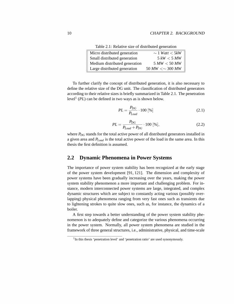
Table 2.1: Relative size of distributed generation
Micro distributed generation ∼ 1 Watt< 5kWSmall distributed generation 5kW < 5 MWMedium distributed generation 5MW < 50MWLarge distributed generation 50MW <∼ 300MW
To further clarify the concept of distributed generation, it is also necessary todefine the relative size of the DG unit. The classification of distributed generatorsaccording to their relative sizes is briefly summarized in Table 2.1. The penetrationlevel1 (PL) can be defined in two ways as is shown below.
PL =PDG
PLoad·100[%] (2.1)
PL =PDG
PLoad+PDG·100[%], (2.2)
wherePDG stands for the total active power of all distributed generators installed ina given area andPLoad is the total active power of the load in the same area. In thisthesis the first definition is assumed.
2.2 Dynamic Phenomena in Power Systems
The importance of power system stability has been recognized at the early stageof the power system development [91, 121]. The dimension and complexity ofpower systems have been gradually increasing over the years, making thepowersystem stability phenomenon a more important and challenging problem. For in-stance, modern interconnected power systems are large, integrated, andcomplexdynamic structures which are subject to constantly acting various (possiblyover-lapping) physical phenomena ranging from very fast ones such as transients dueto lightening strokes to quite slow ones, such as, for instance, the dynamics of aboiler.
A first step towards a better understanding of the power system stability phe-nomenon is to adequately define and categorize the various phenomena occurringin the power system. Normally, all power system phenomena are studied in theframework of three general structures, i.e., administrative, physical, and time-scale
1In this thesis ‘penetration level’ and ‘penetration ratio’ are used synonymously.

2.3. FORMAL DEFINITION OF POWER SYSTEM STABILITY 11
Fault currents
-10−6 10−3 100 103 Time [s]
Lightning transientsSwitching transients
Resonance phenomenaA
Generator transients
Transient stabilityLong term stability
Harmonic distortionPower flow
B
C
D
Figure 2.1: Simplified chart of dynamic phenomena in power systems [18]. ZonesA, B, C, and D denote fast transients, generator dynamics, quasi steady state, andsteady state, respectively.
structures [107]. The administrative structure regulates the political organizationof the power grid, i.e., it establishes the hierarchical structure of variouslayersof the power grid. The physical structure describes the main components of thepower system, relations between them, control equipment, as well as the energyconversion principles. Finally, the time-scale structure categorizes the dynamicphenomena that occur in the power system according to the time scale of the un-derlying physical processes. The latter structure is arguably the most appropriatefor studying the dynamics of the power system and hereby is adopted in this thesis.Figure 2.1 shows an approximate time-scale structure of power system phenomenaof interest, which will be used in this thesis. In general, all the phenomena can bedivided in two large groups corresponding to fast and slow dynamics, dependingon the time scale of the underlying physical processes triggering the mechanismsof power system instability. In the remainder of this chapter various definitions ofpower system stability are presented and discussed.
2.3 Formal Definition of Power System Stability
The concept of stability is one of the most fundamental concepts in most engi-neering disciplines. Due to the devastating impact that instabilities might cause indynamical systems, numerous definitions of stability have been formulated, em-phasizing its various aspects that reflect the manifestation of the system’s stablestate. It is known that over 28 definitions of stability were introduced for technical

12 CHAPTER 2. BACKGROUND
and physical reasons in the systems theory. Some of the definitions might be quiteuseful in one situation, but inadequate in many others. To avoid possible ambi-guities and establish rigorous foundations of the subsequent discussion, the mainemphasis in this thesis is placed upon the so-called stability in the sense of A. M.Lyapunov [103].
Technical assumptions
A1: The power system can in general be satisfactorily described by a set of first-order ordinary differential-algebraic equations (DAE) of the form:
[x0
]
=
[f (t,x,y, p)g(t,x,y, p)
]
= F(t,x,y, p), (2.3)
where variablet ∈ I ⊆ R represents time, the derivative with respect to time isdenoted as ˙x = dx/dt, x∈U ⊆ R
n designates the vector of state variables,y∈ Rm
is the vector of algebraic variables,p∈Rl is the vector of controllable parameters,
f : I ×Rn×R
m×Rl →R
n stands for a certain nonlinear function, andg :×Rn×
Rm×R
l → Rm denotes a nonlinear vector-valued function.
A2: We assume that the Jacobian matrix
Dyg(x,y, p) =∂g∂y
(2.4)
is nonsingular along all the trajectories of (2.3), thus ensuring that the setof DAEcan be reduced to a set of ODE’s by virtue of the Implicit Function Theorem[54,104].A3: It is also assumed that the functionF is sufficiently smooth to ensure ex-istence, uniqueness, and continuous dependence of the solutions of (2.3) on theinitial conditions over the domain ofF .A4: Without loss of generality, it will be assumed that the origin is a critical pointof (2.3).Finally, letBr denote an open ball of radiusr, i.e.,Br = x∈U : ‖x‖< r, where‖ ‖ is any norm andσ stands for the right maximal interval wherex(·, t0,x0, p) isdefined.
Definition 2 Let assumptionsA1–A4 hold. Then, the solution x= 0 is called stableif ∀ε > 0 and∀t0 ∈ I there exists a positive numberδ such that∀x0 ∈Bδ and∀t0 ∈ σ , the following inequality holds:‖x(t, t0,x0, p)‖< ε.
2.3. FORMAL DEFINITION OF POWER SYSTEM STABILITY 13
This definition can be loosely restated in other terms: for every given positive εandt0 ∈I , there exists a positiveδ , which in general is a function ofε, such thatfor all initial values ofx that belong to an open ball of radiusδ , the solutionx(t)remains in an open ball of radiusε for all time.
Definition 3 The system is termed unstable if it is not stable.
Definition 4 The solution x= 0 of system (2.3) is referred to as uniformly stable if∀ε > 0 there exists aδ (ε) > 0 :∀x0∈Bδ and∀t0∈I such that‖x(t, t0,x0, p)‖< ε.
Remark:Stated differently, uniform stability of (2.3) is obtained by relaxing thedependence ofδ on t0.
Definition 5 The solution x= 0 of system (2.3) is called attractive if for each t0 ∈I there is a positive numberη = η(t0), and for each positiveε and‖x(x0, p)‖< ηthere is a positiveω = ω(t0,ε,x0, p) such that t0 + ω ∈ σ and‖x(t, t0,x0, p)‖ < εfor all t ≥ t0 +ω .
Definition 6 The solution x= 0 is asymptotically stable if it is both stable andattractive.
Note: In the definition above it is necessary to require that the system is both stableand attractive, since attractivity does not—in general—imply stability. In otherwords, it is possible to construct an example in which the origin is attractive, i.e.,every solution tends to it ast→ ∞, but yet the origin is unstable [129].
Definition 7 Let x∗ be a hyperbolic equilibrium point. Its stable and unstablemanifolds, Ws(x∗) and Wu(x∗), are defined as follows:
Ws(x∗) = x∈ Rn : Φ(t,x)→ x∗ as t→ ∞
Wu(x∗) = x∈ Rn : Φ(t,x)→ x∗ as t→−∞,
whereΦ(t,x) is the solution of (2.3). Then the stability region (or region/domainof attraction) of a stable equilibrium x∗ is defined as
A(x∗) = x∈ Rn : lim
t→∞Φ(t,x) = x∗.

14 CHAPTER 2. BACKGROUND
Definition 8 If there exists an energy function for system (2.3), then the stabilityboundary∂A(x∗) is contained in the union of the stable manifolds of the unstableequilibria on∂A(x∗). That is,
∂A(x∗)⊆⋃
xi∈∂A(x∗)
Ws(xi),
where xi are the hyperbolic equilibria of (2.3).
Definition 9 The system (2.3) falls into the category of linear systems if F is alinear function.
Most of physical dynamic systems, including power systems, are essentiallynon-linear; however, it has become a common practice to study the local behaviorof theoriginal nonlinear system by linearizing it around an equilibrium point of interest.Then some of the dynamic properties of the nonlinear system can be inferred byanalyzing the corresponding linear model. These properties, however,hold trueonly in some sufficiently small neighborhood of the equilibrium point. To obtainresults that are valid globally, the nonlinear model has to be analyzed.
Definition 10 The system (2.3) is referred to as autonomous if F is not an explicitfunction of time; otherwise it is termed non-autonomous.
Remark:Often studying the dynamic properties of power systems, it is assumedthat the system at hand is autonomous. This assumption allows the use of muchmore simple analytical tools; however, in general, strictly speaking, power systemsare non-autonomous [47].
Some of the presented concepts are further clarified by the following two ex-amples.
Example:Consider the system of 2 nonlinear autonomous differential equations[
x1
x2
]
=
[x2−x1x2
−0.9x1− (x21−0.7)x2
]
. (2.5)
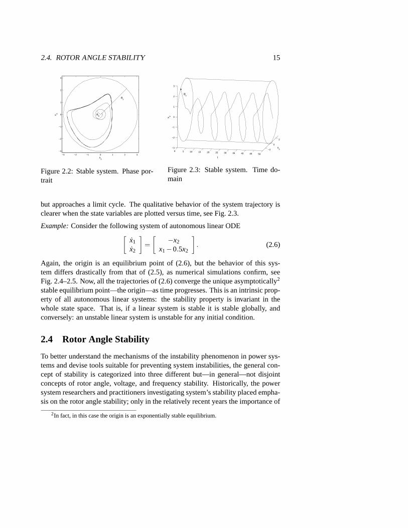
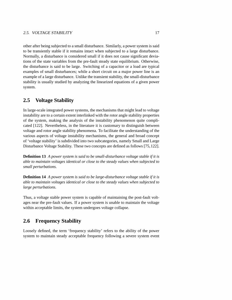
Clearly, the origin is a critical point of (2.5), but no system trajectory convergesto it. However, as the simulations indicate, all the trajectories are bounded forall sufficiently small‖x0‖. Thus, the origin of the system is unstable. Figure 2.2shows the phase portrait of (2.5) for some initial conditions. It can be seen in thefigure that the system trajectory does not converge to a single point in the plane
2.4. ROTOR ANGLE STABILITY 15
−3 −2 −1 0 1 2 3
−3
−2
−1
0
1
2
3
x1
x 2
Bε
Bδ
Figure 2.2: Stable system. Phase por-trait
0 5 10 15 20 25 30 35 40 45 50
−2
0
2
−3
−2
−1
0
1
2
3
x1
t
x 2
Bε
Figure 2.3: Stable system. Time do-main
but approaches a limit cycle. The qualitative behavior of the system trajectory isclearer when the state variables are plotted versus time, see Fig. 2.3.
Example:Consider the following system of autonomous linear ODE[
x1
x2
]
=
[−x2
x1−0.5x2
]
. (2.6)
Again, the origin is an equilibrium point of (2.6), but the behavior of this sys-tem differs drastically from that of (2.5), as numerical simulations confirm, seeFig. 2.4–2.5. Now, all the trajectories of (2.6) converge the unique asymptotically2
stable equilibrium point—the origin—as time progresses. This is an intrinsic prop-erty of all autonomous linear systems: the stability property is invariant in thewhole state space. That is, if a linear system is stable it is stable globally, andconversely: an unstable linear system is unstable for any initial condition.
2.4 Rotor Angle Stability
To better understand the mechanisms of the instability phenomenon in power sys-tems and devise tools suitable for preventing system instabilities, the general con-cept of stability is categorized into three different but—in general—not disjointconcepts of rotor angle, voltage, and frequency stability. Historically, thepowersystem researchers and practitioners investigating system’s stability placedempha-sis on the rotor angle stability; only in the relatively recent years the importance of
2In fact, in this case the origin is an exponentially stable equilibrium.

16 CHAPTER 2. BACKGROUND
−0.1 −0.05 0 0.05 0.1 0.15
−0.1
−0.05
0
0.05
0.1
0.15
x1
x 2
Bδ
Figure 2.4: Asymptotically stable sys-tem. Phase portrait
010
2030
4050
−0.1−0.05
00.05
0.1
−0.1
−0.05
0
0.05
0.1
x1
t
x 2
Bδ
Figure 2.5: Asymptotically stable sys-tem. Time domain
voltage stability was recognized. We therefore commence by quoting the classicaldefinition of power system stability due to E. Kimbark [69]:
Definition 11 Power system stability is a term applied to alternating-current elec-tric power systems, denoting a condition in which the various synchronousma-chines of the system remain in synchronism, or “in step,” with each other.
While this definition is valid and satisfactorily conforms to the system-theoreticdefinitions presented above, a more elaborated definition of power systemstabilitywas proposed in [75]:
Definition 12 Power system stability is the ability of an electric power system, fora given initial operating condition, to regain a state of operating equilibrium afterbeing subjected to a physical disturbance, with most system variables bounded sothat practically the entire system remains intact.
This new definition allows a more subtle distinction between various instabilityscenarios based on the characteristics of the physical disturbance.
It is known that power systems are subject to continuously acting disturbances.The vast majority of them are relatively small, compared to the power system ca-pacity; however, more severe disturbances also occur. Therefore,it is natural tosubdivide the general concept of angle stability to the so-called small-disturbanceand transient stability. Thus, a power system is termed stable in the sense of small-disturbance stability if the system’s generators are able to remain in step with each
2.5. VOLTAGE STABILITY 17
other after being subjected to a small disturbance. Similarly, a power system issaidto be transiently stable if it remains intact when subjected to a large disturbance.Normally, a disturbance is considered small if it does not cause significantdevia-tions of the state variables from the pre-fault steady state equilibrium. Otherwise,the disturbance is said to be large. Switching of a capacitor or a load are typicalexamples of small disturbances; while a short circuit on a major power line is anexample of a large disturbance. Unlike the transient stability, the small-disturbancestability is usually studied by analyzing the linearized equations of a given powersystem.
2.5 Voltage Stability
In large-scale integrated power systems, the mechanisms that might lead to voltageinstability are to a certain extent interlinked with the rotor angle stability propertiesof the system, making the analysis of the instability phenomenon quite compli-cated [122]. Nevertheless, in the literature it is customary to distinguish betweenvoltage and rotor angle stability phenomena. To facilitate the understanding ofthevarious aspects of voltage instability mechanisms, the general and broad conceptof ‘voltage stability’ is subdivided into two subcategories, namely Small and LargeDisturbance Voltage Stability. These two concepts are defined as follows [75,122].
Definition 13 A power system is said to be small-disturbance voltage stable if it isable to maintain voltages identical or close to the steady values when subjectedtosmall perturbations.
Definition 14 A power system is said to be large-disturbance voltage stable if it isable to maintain voltages identical or close to the steady values when subjectedtolarge perturbations.
Thus, a voltage stable power system is capable of maintaining the post-fault volt-ages near the pre-fault values. If a power system is unable to maintain the voltagewithin acceptable limits, the system undergoes voltage collapse.
2.6 Frequency Stability
Loosely defined, the term ‘frequency stability’ refers to the ability of the powersystem to maintain steady acceptable frequency following a severe system event

18 CHAPTER 2. BACKGROUND
resulting in a large generation-load imbalance. Technically, the frequencystabil-ity is a system-wide phenomenon which primarily depends on the overall systemresponse to the event and the availability of substantial power reserves.
It is not very likely that distributed generation will have significant impact onthefrequency stability phenomenon in the near future; due to this fact, the frequencystability phenomenon is not studied in this thesis.
2.7 Summary
It can be noted that the definitions of voltage stability follow closely those of therotor angle. Analogously, the analytical tools for studying the voltage stabilityphenomena are the same. That is, the small-disturbance stability can be effec-tively studied with the help of linearized models of the power system. Inspectionof the eigenvalues of the state matrix provides sufficient information regarding thesmall-disturbance voltage stability of the power system in some neighborhood of agiven operating point. On the other hand, the investigation of the large-disturbancevoltage stability properties of the power grid, requires the use of nonlinearsystemanalysis. This observation concludes the presentation of the various stability def-initions relevant to the work presented in this thesis. The next section will brieflypresent modeling issues of such power system components as the synchronous andasynchronous generators, and solid oxide fuels cells.
Chapter 3
Power System Modeling
“All these constructions and the laws connecting themcan be arrived at by the principle of looking
for the mathematically simplest conceptsand the link between them.”
— A. Einstein.
“Obtaining maximum benefits from installed assets on an interconnected powersystem is becoming increasingly dependent on the coordinated use of automaticcontrol systems. The ability to optimize the configuration of such control devicesand their settings is dependent on having an accurate power system model, as wellas controllers themselves”[5].This compendious but neat quotation form a CIGRE report is cited here to signifythe importance of having an accurate model of the system studied. Indeed,thedevelopment of an adequate model of the process is an essential part ofengineeringwork. This chapter is therefore devoted to describing the basic models of somerelevant power system components.
3.1 Main Components of Power SystemsThe modern power systems are characterized by growing complexity andsize. For example, the energy consumption in India doubles every 10years, which also applies to some other countries [87]. As the dimen-
sions of the power systems increase, the dynamical processes are becoming morecomplicated for analysis and understanding the underlying physical phenomena.In addition to the complexity and size, power systems do exhibit nonlinear andtime-varying behavior.
In an electrical system the power cannot be stored1, at each time instant thereshould be a balance between the total produced and consumed power. Mathe-
1There are some exceptions e.g., a pump storage; however in thoseenergyrather thanpowerisstored.
19

20 CHAPTER 3. POWER SYSTEM MODELING
matically this balance is expressed by differential and algebraic equations.Thepresence of algebraic equations significantly complicates both analytical and com-putational aspects of work when tackling with power systems.
To obtain a meaningful model of the power system, each component of thepower system should be described by appropriate equations be it algebraic equa-tions, differential equations, or both. For example, there are differentmodels ofan electrical generator; depending on the application a model of suitable exactnessand complexity should be chosen to represent the generator in the study. On the onehand, very simple models of a generator are rarely used in power system studieswhen accuracy of the results is a great concern. On the other hand, if asystem con-sists of 300 generators, each modeled by a set of three differential equations, thesystem analyst would have to process at least 900 differential equations describingthe system as well as quite a few algebraic equations, the number of which de-pends on the topology of the network. The presence of other equipment, e.g., highvoltage direct current (HVDC) systems, further contributes to the aforementionednumber of equations. Clearly, it is barely possible to carry out any analytical studyon such systems.
To overcome the problem of high dimension, the order of the system has to bereduced. This can be done in several ways:
• Based on the physical insights, several generators are aggregated ina groupof coherent generators [88].
• Having set up the system equations, one applies a model reduction techniqueand eliminates the states that have little effect on the system dynamics [88].
• Using field measurements, one applies a system identification technique toobtain an equivalent model of the system [79].
Depending on the case study, any of the methods or a combination of them canbeused to obtain ‘best’ dynamical models.
Linear and Nonlinear Systems
As was already mentioned, the nature of power systems is essentially nonlinear.Mathematically speaking, nonlinear systems are known to be very hard to manage.To work around this problem, when studying the behavior of a power system in aneighborhood of an equilibrium point, it is a common assumption that the powersystem is a linear, time-invariant system [101]. That is, the initial nonlinear sys-tem is approximated by a linear one. In many cases of practical importance, this

3.1. MAIN COMPONENTS OF POWER SYSTEMS 21
assumption works quite well yielding numerous advantages. However, when tran-sient stability of the system is investigated, the use of a linear model may not bejustified. There are several reasons for questioning the validity of the linear model;the main reason is the dependence of the qualitative behavior of a nonlinearmodelon the level of disturbance. This statement is further illustrated by the following
Example:Consider the following two systems described by second order homoge-nous differential equations (DE)
x1(t)+0.01x1(t)+x1(t) = 0, (3.1)
x2(t)+0.01x2(t)+sinx2(t) = 0. (3.2)
Equation (3.1) is a linear DE, while (3.2) is a nonlinear differential equation.Wenow determine the qualitative behavior of the solutions of (3.1) and (3.2).
Since the first equation is a linear equation with the eigenvalues having negativereal part (ℜ(λ1,2) = −1/200), the domain of attraction is the whole plane. Thismeans, for any choice of initial state of the system, the system state variables willalways converge to the origin. This is confirmed by the explicit solution of (3.1)
x1(t) = exp(−t/200)Csin(ω1t +φ) ,
whereω1 is the imaginary part of the eigenvalue, the constantsC andφ are deter-mined by initial conditions. Clearly, lim
t→∞x1(t) = 0,∀C,φ .
Now equation (3.2) is examined. Despite its apparent simplicity, there existsno closed-form solution to this equation. The difficulty in finding closed-formsolutions to nonlinear differential equations2 has stimulated the search for othermethods which allow the analyst to obtain a qualitative characteristics of a solutionwithout actually having to solve the equation.
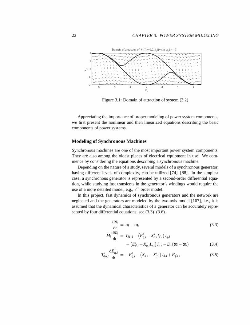
For the moment, this approach will not be pursued, instead the domain of at-traction of this system will be found. This is done by integrating the equationbackwards in time [128]. The domain of attraction3 is the region which includesthe origin, see Fig. 3.1. If the initial state of the system was chosen inside the re-gion, the system states will eventually converge to the origin, otherwise the originwill never be reached. It is evident that for small deviations from the origin, equations (3.1) and (3.2) areequivalent (sinx≈ x); as the deviations grow in magnitude, the difference in the be-havior becomes more expressed. This example concludes the notes on qualitativedifference between linear and nonlinear models.
2Only in some exceptional cases there exist closed-form solutions to nonlinear systems [127].3The Bendixson theorem indicates that this domain is open.
22 CHAPTER 3. POWER SYSTEM MODELING
-6 -4 -2 0 2 4 6-2
-1
0
1
2
x2
x 2
x
..
2 ) + 0.01t(Domain of attraction of x
2(t()+ sin
2x t) = 0.
.
Figure 3.1: Domain of attraction of system (3.2)
Appreciating the importance of proper modeling of power system components,we first present the nonlinear and then linearized equations describing the basiccomponents of power systems.
Modeling of Synchronous Machines
Synchronous machines are one of the most important power system components.They are also among the oldest pieces of electrical equipment in use. We com-mence by considering the equations describing a synchronous machine.
Depending on the nature of a study, several models of a synchronous generator,having different levels of complexity, can be utilized [74], [88]. In the simplestcase, a synchronous generator is represented by a second-orderdifferential equa-tion, while studying fast transients in the generator’s windings would require theuse of a more detailed model, e.g., 7th order model.
In this project, fast dynamics of synchronous generators and the network areneglected and the generators are modeled by the two-axis model [107], i.e.,it isassumed that the dynamical characteristics of a generator can be accurately repre-sented by four differential equations, see (3.3)–(3.6).
dδi
dt= ωi−ωs (3.3)
Midωi
dt= TM, i−
(E′q,i−X′d,i Id,i
)Iq,i
−(E′d,i +X′q,i Iq,i
)Id,i−Di (ωi−ωs) (3.4)
T ′do,i
dE′q,i
dt= −E′q,i−
(Xd,i−X′d,i
)Id,i +Ef d,i (3.5)
3.1. MAIN COMPONENTS OF POWER SYSTEMS 23
T ′do,i
dE′d,i
dt= −E′d,i−
(Xq,i−X′q,i
)Iq,i (3.6)
In the equations above, the following symbols are used to denote:
• δi : The rotor shaft angle of theith generator. Normally this angle is expressedin radians or degrees.
• ωi ,ωs: The rotor angular velocity of theith generator. This velocity is com-monly expressed in radians per second or per unit.ωs is the synchronousspeed of the system which usually takes two valuesωs = 100π,(120π) radi-ans per second.
• Mi : The shaft inertia constant of theith generator which has the units ofseconds squared.
• TM,i : The mechanical torque applied to the shaft of theith generator.
• E′q,i ,E′d,i : These symbols denominate the transient EMF’s of the machine in
theq andd axes, respectively.
• Iq,i , Id,i : Are the equivalent currents of the synchronous machine in theq andd axes, respectively.
• Di : The damping coefficient of theith generator.
• T ′do,i ,T′qo,i : Are transient time constants of the open circuit and a damper
winding in theq-axis. These time constants are commonly expressed inseconds.
• Xq,i ,Xd,i ,X′q,i ,X′d,i : These four symbols stand for the synchronous reactance
and transient synchronous reactance of theith machine.
Sometimes equation (3.6) is eliminated yielding the third-order model of the syn-chronous generator. In the equations above, the indexi runs from 1 ton, wheren isthe number of synchronous generators in the system. In our case studies, the num-ber of synchronous machines does not exceed 2; yet in many studies thisnumbermay exceed several hundred.

24 CHAPTER 3. POWER SYSTEM MODELING
Modeling the excitation system
Control of the excitation system of a synchronous machine has a very strong in-fluence on its performance, voltage regulation, and stability [34]. Not onlyis theoperation of a single machine affected by its excitation, but also the behaviorofthe whole system is dependent on the excitation system of separate generators. Forexample, inter-area oscillations are directly connected to the excitation of separategenerators [71]. These are only a few arguments justifying the necessityfor accu-rate and precise modeling of the excitation system of a synchronous machine. Thissubsection therefore presents the modeling principles of the excitation system. Adetailed treatment of all aspects of the modeling is far beyond the scope of thethesis; we only synoptically present a literature survey on the subject.
There are different types of excitation systems commercially available in powerindustry. However, one of the most commonly encountered models is the so-called“IEEE Type DC1” excitation system. The main equations describing this modelare listed below.
TE,idEf d,i
dt= −
(KE,i +SE,i
(Ef d,i
))Ef d,i +VR,i (3.7)
TA,idVR,i
dt= −VR,i +KA,iRf ,i−
KA,iKF,i
TF,iEf d,i
+KA,i (Vre f,i−Vi) (3.8)
TF,idRf ,i
dt= −Rf ,i +
KF,i
TF,iEf d,i (3.9)
In these equations, the parameters and variables used are:
• TE,i ,KE,i ,Ef d,i ,SE,i ,: Time constant, gain, field voltage, and saturation func-tion of the excitor.
• VR,i ,TA,i ,KA,i : Exciter input voltage, time constant and gain of the voltageregulator (amplifier), respectively.
• Vre f,i ,Vi : The reference and actual voltage of theith node.
• Rf ,i ,KF,i ,TF,i : Transient gain reduction circuit parameters—state, gain, andtime constant.
A block diagram of the exciter given by equations (3.7)–(3.9) is shown in Fig. 3.2.As is evident from (3.7)–(3.9), each excitor of the type DC1 adds three state vari-ables to the state matrix.
3.1. MAIN COMPONENTS OF POWER SYSTEMS 25
Stabilizingfeedback
1
E EK sT+FDE∆RV
Voltage regulatorrefV
ΣtV+
1A
A
K
sT+
1F
F
sK
sT+
−−
Exciter
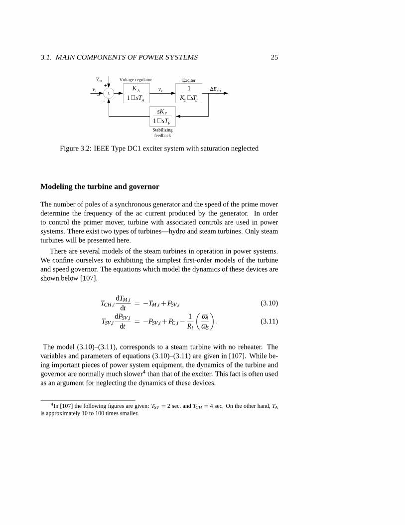
Figure 3.2: IEEE Type DC1 exciter system with saturation neglected
Modeling the turbine and governor
The number of poles of a synchronous generator and the speed of the prime moverdetermine the frequency of the ac current produced by the generator.In orderto control the primer mover, turbine with associated controls are used in powersystems. There exist two types of turbines—hydro and steam turbines. Only steamturbines will be presented here.
There are several models of the steam turbines in operation in power systems.We confine ourselves to exhibiting the simplest first-order models of the turbineand speed governor. The equations which model the dynamics of these devices areshown below [107].
TCH,idTM,i
dt= −TM,i +PSV,i (3.10)
TSV,idPSV,i
dt= −PSV,i +PC,i−
1Ri
(ωi
ωS
)
. (3.11)
The model (3.10)–(3.11), corresponds to a steam turbine with no reheater. Thevariables and parameters of equations (3.10)–(3.11) are given in [107]. While be-ing important pieces of power system equipment, the dynamics of the turbine andgovernor are normally much slower4 than that of the exciter. This fact is often usedas an argument for neglecting the dynamics of these devices.
4In [107] the following figures are given:TSV = 2 sec. andTCH = 4 sec. On the other hand,TAis approximately 10 to 100 times smaller.

26 CHAPTER 3. POWER SYSTEM MODELING
Asynchronous Generators
It is known that the essential dynamical properties of an asynchronousgeneratorcan be accurately described by the following model [73]
1ωs
dψds
dt= −
rsxrr
Dψds−ψqs+
rsxm
Dψdr +vds
1ωs
dψqs
dt= ψds−
rsxrr
Dψqs+
rsxm
Dψqr +vqs
1ωs
dψdr
dt= −
rrxss
Dψdr +
rrxm
Dψds−
ωs−ωr
ωsψqr + vdr
1ωs
dψqr
dt= −
rrxss
Dψqr +
rrxm
Dψqs+
ωs−ωr
ωsψdr + vqr
dωr
dt=
ωs
2H(Tm−Te) , (3.12)
wherexss= xs+xm, xrr = xr +xm, D = xssxrr −x2m, Te = xm(ψqsψdr−ψdsψqr)/D.
xr andxs stand for the rotor and stator leakage reactances, respectively.xm andωr signify the magnetizing reactance and the mechanical rotor angular frequency.The state variablesψds,ψqs,ψdr, andψqr are thed andq components of the statorand rotor flux linkages per second. [Note that the explicit dependence of the statevariables on time is suppressed for notational ease.]rs andrr are the stator and rotorresistances, respectively.ωs = 2π f0, where f0 is the steady-state grid frequency(50 or 60 Hz.) Finally,vds (vdr) andvqs (vqr) denote thed andq components of thestator (rotor) voltage. Unless otherwise specified, all the quantities are given in perunit. For more details on the model (3.12), the reader can refer to [73].
Neglecting the asynchronous generator’s stator dynamics, i.e., assuming thatω−1
s dψds/dt = 0,ω−1s dψqs/dt = 0 and that the stator resistance is negligibly small,
the following model of the asynchronous generator is obtained [23]:
dψdr
dt= ωs
[
−rrxss
Dψdr +
rrxm
Dvqs+
ωs−ωr
ωsψqr + vdr
]
dψqr
dt= ωs
[
−rrxss
Dψqr−
rrxm
Dvdsωs−
ωs−ωr
ωsψdr + vqr
]
(3.13)
dωr
dt=
ωs
2H(Tm−Te) .
Introducing the constantsvdr = ωsvdr,vqr = ωsvqr, a1 = rrxmωs/D,a2 = rrxssωs/Dand denoting the state variablesx1 = ψdr,x2 = ψqr,x3 = ω = ωr −ωs, we arrive at
3.1. MAIN COMPONENTS OF POWER SYSTEMS 27
the reduced-order model of the asynchronous generator:
dx1
dt= −a2x1 +x2x3 +a1vqs−vdr
dx2
dt= −a2x2−x1x3−a1vds−vqr (3.14)
dx3
dt= c1 +c2(vdsx1 +vqsx2)
wherec1 = ωsTm/(2H) andc2 =−a1/(2Hrr).The steady state of the asynchronous generator is characterized by theequilib-
rium pointx∗= [x∗1,x∗2,x∗3]′ which renders the right-hand side of (3.14) zero5. There
are 2 such points:
x∗1 =1
2a2c2v2s[vqs[c2p3± p4]−2a2c1vds]
x∗2 =−1
2a2c2v2s[c2p3± p4 +2a2c1] (3.15)
x∗3 =1
2c1[c2p3± p4] ,
where the constantsp1, . . . , p4 are defined as follows:p1 = vdsvqr− vqsvdr, p2 =
vdsvdr +vqsvqr, p3 = a1v2s + p1, andp4 =
√
c22p2
3 +4a2c1c2p2−4a22c2
1. One of thepoints is asymptotically stable, while the second is unstable. For convenience ofthe analytical explorations presented in this section, the stable equilibrium point ofthe model (3.14) is translated to the origin by means of the change of coordinatesξ1 := x1−x∗1,ξ2 := x2−x∗2,ξ3 := x3−x∗3. This operation yields the model:
ξ1 = −a2ξ1 +x∗3ξ2 +x∗2ξ3 +ξ2ξ3
ξ2 = −a2ξ2−x∗3ξ1−x∗1ξ3−ξ1ξ3 (3.16)
ξ3 = c2vdsξ1 +c2vqsξ2.
Note that the model (3.16) can be decomposed into two parts: linear and nonlinear.That is,
ξ =
−a2 x∗3 x∗2−x∗3 −a2 −x∗1c2vds c2vqs 0
ξ +
ξ2ξ3
−ξ1ξ3
0
, (3.17)
5In this thesis the prime denotes the transposition operator, unless explicitly stated otherwise.
28 CHAPTER 3. POWER SYSTEM MODELING
Fuel in
2H
2H O
Depleted fuel
Oxidant
in
Positive ion
Negative ion
Electrolyte
2O
2H O
Depleted
oxidant
Anode Cathode
Electric load
Current
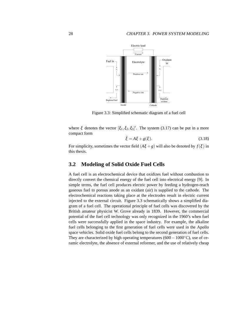
Figure 3.3: Simplified schematic diagram of a fuel cell
whereξ denotes the vector[ξ1,ξ2,ξ3]′. The system (3.17) can be put in a more
compact formξ = Aξ +g(ξ ). (3.18)
For simplicity, sometimes the vector field(Aξ +g) will also be denoted byf (ξ ) inthis thesis.
3.2 Modeling of Solid Oxide Fuel Cells
A fuel cell is an electrochemical device that oxidizes fuel without combustion todirectly convert the chemical energy of the fuel cell into electrical energy [9]. Insimple terms, the fuel cell produces electric power by feeding a hydrogen-reachgaseous fuel to porous anode as an oxidant (air) is supplied to the cathode. Theelectrochemical reactions taking place at the electrodes result in electric currentinjected to the external circuit. Figure 3.3 schematically shows a simplified dia-gram of a fuel cell. The operational principle of fuel cells was discovered by theBritish amateur physicist W. Grove already in 1839. However, the commercialpotential of the fuel cell technology was only recognized in the 1960’s when fuelcells were successfully applied in the space industry. For example, the alkalinefuel cells belonging to the first generation of fuel cells were used in the Apollospace vehicles. Solid oxide fuel cells belong to the second generation of fuel cells.They are characterized by high operating temperatures (600−1000C), use of ce-ramic electrolyte, the absence of external reformer, and the use of relatively cheap
3.2. MODELING OF SOLID OXIDE FUEL CELLS 29
catalysts. The high operating temperatures of SOFC result in a high temperatureexhaust which can be utilized to increase the overall efficiency of the process. Inrecent years, the combined use of SOFC and a small-scale gas turbine (GT) or “mi-croturbine” has been actively discussed. Analysis and experiments show that veryhigh efficiencies (over 80%) can be achieved if the hot exhaust from the fuel cellis used to power a gas turbine [9]. It is argued in [9] and [126] that the capacity ofthe microturbine should be at most one third of the capacity of the SOFT/GT sys-tem. The technical and economical advantages of SOFC/GT systems make themattractive energy sources for distributed generation.
In addition to generating electric power at high efficiency, the SOFC/GT baseddistribution generation can also provide ancillary services such as load follow-ing and regulation. The technical feasibility of load following functionality ofSOFT/GT systems is investigated in [135]. The numerical experiment results pro-vided in [135] indicate that the fuel cell response times are significantly greaterthan those of the GT used in that study. This result implies that the GT rather thanthe fuel cells should be deployed in load following. The active power set-point ofthe fuel cell should only be adjusted when it is needed to substantially alter thenet output of the SOFC/GT system. In this chapter, the main emphasis is placedupon the control challenges of the fuel cell rather than the dynamic properties ofthe microturbine; therefore, no dynamic model of the microturbine are developed.The presence of the microturbine will be indirectly accounted for by modelingthevoltage deviations caused by the operation of the microturbine in the analysespre-sented here.
Fuel cell systems have to be interfaced with the distribution grid by means of apower converter, since the fuel cells produce dc power which has to beconvertedto ac. Normally, a forced-commutated voltage source inverter (VSI) is utilizedfor interfacing a fuel cell system. It is known that a VSI can provide fast andprecise control of the voltage magnitude and reactive power output of theSOFT/GTsystem [85]. We, therefore, assume that the fuel cell power plant is equipped with aVSI, whose internal voltage control loops ensure an accurate controlof ac voltagemagnitude; it is also assumed that the converter losses can be neglected andthat thetime constants of the control are small enough to not be taken into account here.
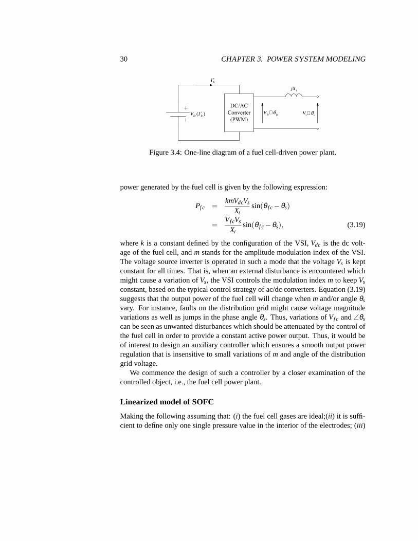
Figure 3.4 depicts a one-line diagram of the fuel cell power plant along withits power conditioning unit (VSI). In this figure,Vf c∠θ f c denotes the ac voltage ofthe VSI. Although not mentioned explicitly, we assume that the fuel cell plant isconnected to the distribution grid via a transformer which is represented in Fig. 3.4by its leakage reactanceXt ; thus,Vs∠θs is the voltage of secondary winding of thetransformer representing the bus voltage of the fuel cell. In this case, theactive
30 CHAPTER 3. POWER SYSTEM MODELING
DC/AC
Converter
(PWM)( )r
dc fcV I fc fcV θ∠
rfcI
s sV θ∠
tjX
Figure 3.4: One-line diagram of a fuel cell-driven power plant.
power generated by the fuel cell is given by the following expression:
Pf c =kmVdcVs
Xtsin(θ f c−θs)
=Vf cVs
Xtsin(θ f c−θs), (3.19)
wherek is a constant defined by the configuration of the VSI,Vdc is the dc volt-age of the fuel cell, andm stands for the amplitude modulation index of the VSI.The voltage source inverter is operated in such a mode that the voltageVs is keptconstant for all times. That is, when an external disturbance is encountered whichmight cause a variation ofVs, the VSI controls the modulation indexm to keepVs
constant, based on the typical control strategy of ac/dc converters. Equation (3.19)suggests that the output power of the fuel cell will change whenm and/or angleθs
vary. For instance, faults on the distribution grid might cause voltage magnitudevariations as well as jumps in the phase angleθs. Thus, variations ofVf c and∠θs
can be seen as unwanted disturbances which should be attenuated by the control ofthe fuel cell in order to provide a constant active power output. Thus, itwould beof interest to design an auxiliary controller which ensures a smooth output powerregulation that is insensitive to small variations ofm and angle of the distributiongrid voltage.
We commence the design of such a controller by a closer examination of thecontrolled object, i.e., the fuel cell power plant.
Linearized model of SOFC
Making the following assuming that: (i) the fuel cell gases are ideal;(ii ) it is suffi-cient to define only one single pressure value in the interior of the electrodes; (iii )
3.2. MODELING OF SOLID OXIDE FUEL CELLS 31
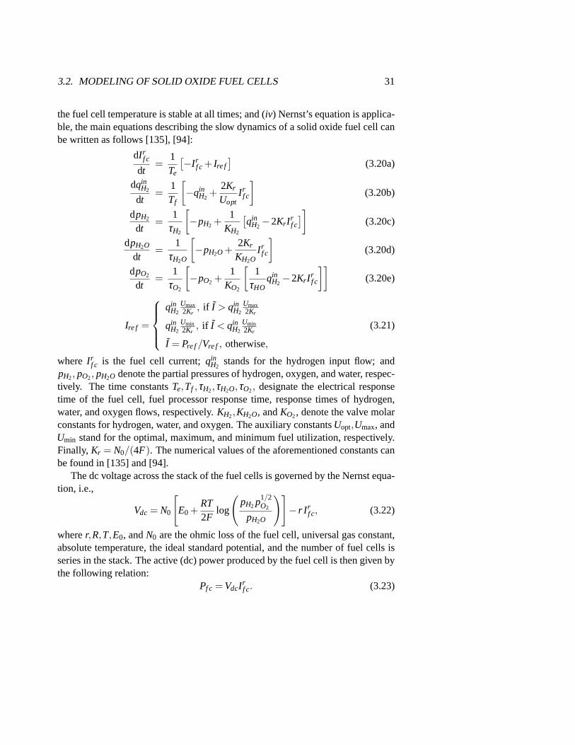
the fuel cell temperature is stable at all times; and (iv) Nernst’s equation is applica-ble, the main equations describing the slow dynamics of a solid oxide fuel cell canbe written as follows [135], [94]:
dI rf c
dt=
1Te
[−I r
f c + Ire f]
(3.20a)
dqinH2
dt=
1Tf
[
−qinH2
+2Kr
UoptI r
f c
]
(3.20b)
dpH2
dt=
1τH2
[
−pH2 +1
KH2
[qin
H2−2Kr I
rf c
]]
(3.20c)
dpH2O
dt=
1τH2O
[
−pH2O +2Kr
KH2OI r
f c
]
(3.20d)
dpO2
dt=
1τO2
[
−pO2 +1
KO2
[1
τHOqin
H2−2Kr I
rf c
]]
(3.20e)
Ire f =
qinH2
Umax2Kr
, if I > qinH2
Umax2Kr
qinH2
Umin2Kr
, if I < qinH2
Umin2Kr
I = Pre f/Vre f , otherwise,
(3.21)
where I rf c is the fuel cell current;qin
H2stands for the hydrogen input flow; and
pH2, pO2, pH2O denote the partial pressures of hydrogen, oxygen, and water, respec-tively. The time constantsTe,Tf ,τH2,τH2O,τO2, designate the electrical responsetime of the fuel cell, fuel processor response time, response times of hydrogen,water, and oxygen flows, respectively.KH2,KH2O, andKO2, denote the valve molarconstants for hydrogen, water, and oxygen. The auxiliary constantsUopt,Umax, andUmin stand for the optimal, maximum, and minimum fuel utilization, respectively.Finally, Kr = N0/(4F). The numerical values of the aforementioned constants canbe found in [135] and [94].
The dc voltage across the stack of the fuel cells is governed by the Nernst equa-tion, i.e.,
Vdc = N0
[
E0 +RT2F
log
(
pH2 p1/2O2
pH2O
)]
− r I rf c, (3.22)
wherer,R,T,E0, andN0 are the ohmic loss of the fuel cell, universal gas constant,absolute temperature, the ideal standard potential, and the number of fuel cells isseries in the stack. The active (dc) power produced by the fuel cell is then given bythe following relation:
Pf c = VdcIrf c. (3.23)

32 CHAPTER 3. POWER SYSTEM MODELING
Σ?
- -×
÷-- Limit - 1
1+Tr s
Umax2Kr
Umin2Kr
2Kr
Σ
?
?
1rH O
1/KH2O
1+τH2Os
-
-11+Tf s
2KrUopt
-
1/KH21+τH2s
? ?1/KO21+τO2s
Σ-
?
Kr
?
?r
N0
[
E0 + RT2F ln
pH2 p1/2O2
pH2O
]? ? ?
Σ-?
?
×
---
--Pe
Qe
-
∆P
Pre f
V inf c
qinH2
qinH2
-I rf c
qinH2
pH2 pH2O pO2
Vrf c
I rf c
cosφ
I rf c
qinO2
–
–
–
–
Figure 3.5: SOFC system block diagram
The dynamic equations (3.20) of the fuel cell are linear; the only nonlinearities inthese expressions are in the stack voltage and the active power equations. The blockdiagram of the SOFC plant with its basic auxiliary controls is shown in Fig. 3.5.
To obtain the complete linear model, equations (3.19), (3.22), and (3.23) haveto be linearized about the equilibrium point. The resulting linear model contains5state variables and can be represented by
x(t) = Ax(t)+Bu(t) (3.24)
y(t) = Cx(t)+Du(t), (3.25)
wherex = [∆I rf c,∆qin
H2,∆pH2,∆pH2O,∆pO2]
′ (here, a prime denotes transposition).For convenience of notation, in the remainder of the chapter, the symbol∆ is omit-ted for simplicity, but small deviations from the equilibrium are assumed. Also, theexplicit dependence of the plant states, inputs, and outputs on time is suppressedfor simplicity of notation. The state matrixA∈ R
5×5 can be easily extracted fromthe dynamic equations (3.20);B ∈ R
5×3; C ∈ R1×5; andD ∈ R
1×3 are the input,output, and direct feedthrough matrix (their numerical values are given inthe Ap-pendix). The input vector and the output are denoted byu = [∆m,∆θs,∆Pre f ]
′ andy = Pf c, respectively.
3.3. ALGEBRAIC CONSTRAINTS IN POWER SYSTEMS 33
3.3 Algebraic Constraints in Power Systems
As was briefly explained in Section 3.1 on page 20, the power systems are de-scribed by a set of differential and algebraic equations. The origins ofthe differen-tial equations have already been discussed, while those of the algebraic equationsare the main subject of this section.
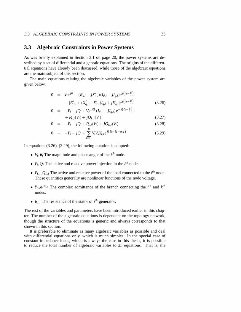
The main equations relating the algebraic variables of the power system aregiven below.
0 = Viejθi +(Rs,i + jX ′d,i)(Id,i + jIq,i)e
j(δi−π2)−
− [E′d,i +(X′q,i−X′d,i)Iq,i + jE ′q,i ]ej(δi−
π2) (3.26)
0 = −Pi− jQi +Viejθi (Id,i− jIq,i)e− j(δi−
π2) +
+PL,i(Vi)+ jQL,i(Vi) (3.27)
0 = −Pi− jQi +PL,i(Vi)+ jQL,i(Vi) (3.28)
0 = −Pi− jQi +n
∑k=1
ViVkYi,kej(θi−θk−αi,k) (3.29)
In equations (3.26)–(3.29), the following notation is adopted:
• Vi ,θi The magnitude and phase angle of theith node.
• Pi ,Qi The active and reactive power injection in theith node.
• PL,i ,QL,i The active and reactive power of the load connected to theith node.These quantities generally are nonlinear functions of the node voltage.
• Yi,kejαi,k The complex admittance of the branch connecting theith and kth
nodes.
• Rs,i The resistance of the stator ofith generator.
The rest of the variables and parameters have been introduced earlier inthis chap-ter. The number of the algebraic equations is dependent on the topology network,though the structure of the equations is generic and always corresponds to thatshown in this section.
It is preferable to eliminate as many algebraic variables as possible and dealwith differential equations only, which is much simpler. In the special case ofconstant impedance loads, which is always the case in this thesis, it is possibleto reduce the total number of algebraic variables to 2n equations. That is, the
34 CHAPTER 3. POWER SYSTEM MODELING
only remaining variables are the complex nodal voltages. To eliminate the statorcurrents one has to solve equation (3.26) forIq,i andId,i . After some manipulation,the following expressions are obtained:
Iq, i =−X′d, iVi sin(θi−δi)+ViRs, i cos(θi−δi)+X′d, iE
′d, i−E′q, iRs, i
X′d, iX′q, i +R2
s, i
(3.30)
Id, i =ViRs, i sin(θi−δi)+E′d, iRs, i−X′q, iVi cos(θi−δi)+X′q, iE
′q, i
X′d, iX′q, i +R2
s, i
(3.31)
Having done this, one can substitute equations (3.30) and (3.31) into (3.26)–(3.29).Moreover, one could reduce the number of algebraic states by eliminating theactiveP and reactiveQ power from equations (3.26) – (3.29).

Chapter 4
Energy Function Analysis ofMixed Power Systems
“. . . But in this respect hardly any other method of investigationcould be said to be completely satisfactory.”
— A. A. LyapunovOn the generality of his method.
The Direct Lyapunov Method is one of the most powerful and well understood ana-lytical tools for investigating the dynamic properties of electric power systemsandother nonlinear systems. Lyapunov’s method establishes a uniform framework forthe assessment of stability of the power system by analyzing an appropriate Lya-punov or energy function. The main advantages of the Lyapunov methodare thepossibility to perform parametric stability studies and the feasibility to concludestability without having to solve the nonlinear differential equations describingthesystem. On the other hand, a practical application of the Lyapunov theoryto tran-sient stability analysis is often a nontrivial task, since finding a suitable Lyapunovfunction is almost always a challenge. To overcome the difficulties inherentin theclassical Lyapunov theory, the so-called Extended Invariance Principle (EIP) canbe considered [25]. The Extended Invariance Principle is an importantextensionof LaSalle’s invariance principle which is in turn an extension of Lyapunov’s directmethod. A function satisfying the conditions of the Extended Invariance Principleis called an extended Lyapunov function. This chapter briefly presents thebasicconcepts of Lyapunov’s direct method and the Extended Invariance Principle andreports the main findings of this thesis related to the transient stability analysis ofpower systems with asynchronous generators.
35
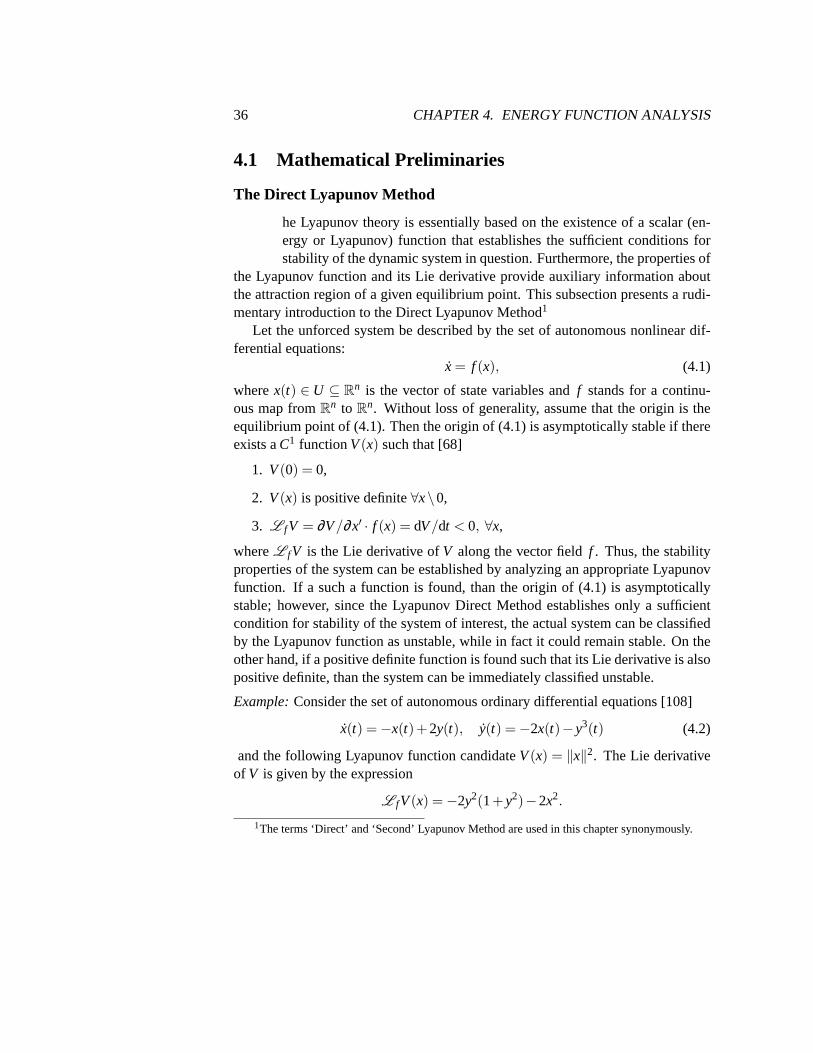
36 CHAPTER 4. ENERGY FUNCTION ANALYSIS
4.1 Mathematical Preliminaries
The Direct Lyapunov MethodThe Lyapunov theory is essentially based on the existence of a scalar (en-ergy or Lyapunov) function that establishes the sufficient conditions forstability of the dynamic system in question. Furthermore, the properties of
the Lyapunov function and its Lie derivative provide auxiliary information aboutthe attraction region of a given equilibrium point. This subsection presents arudi-mentary introduction to the Direct Lyapunov Method1
Let the unforced system be described by the set of autonomous nonlinear dif-ferential equations:
x = f (x), (4.1)
wherex(t) ∈ U ⊆ Rn is the vector of state variables andf stands for a continu-
ous map fromRn to R
n. Without loss of generality, assume that the origin is theequilibrium point of (4.1). Then the origin of (4.1) is asymptotically stable if thereexists aC1 functionV(x) such that [68]
1. V(0) = 0,
2. V(x) is positive definite∀x\0,
3. L fV = ∂V/∂x′ · f (x) = dV/dt < 0, ∀x,
whereL fV is the Lie derivative ofV along the vector fieldf . Thus, the stabilityproperties of the system can be established by analyzing an appropriate Lyapunovfunction. If a such a function is found, than the origin of (4.1) is asymptoticallystable; however, since the Lyapunov Direct Method establishes only a sufficientcondition for stability of the system of interest, the actual system can be classifiedby the Lyapunov function as unstable, while in fact it could remain stable. Ontheother hand, if a positive definite function is found such that its Lie derivative is alsopositive definite, than the system can be immediately classified unstable.
Example:Consider the set of autonomous ordinary differential equations [108]
x(t) =−x(t)+2y(t), y(t) =−2x(t)−y3(t) (4.2)
and the following Lyapunov function candidateV(x) = ‖x‖2. The Lie derivativeof V is given by the expression
L fV(x) =−2y2(1+y2)−2x2.
1The terms ‘Direct’ and ‘Second’ Lyapunov Method are used in this chapter synonymously.

4.1. MATHEMATICAL PRELIMINARIES 37
Clearly, bothV and−L fV are positive definite in the whole state space, whichestablishes global asymptotic stability of (4.2) ‘in-the-large’.
Example:Consider the set of autonomous linear differential equations
x = Ax, (4.3)
whereA∈ Rn×n has distinct eigenvaluesλi
n1. Changing the coordinates by the
similarity transformationz= Tx, whereT is the matrix of right eigenvalues ofA,the system (4.3) can be transformed to diagonal form
z= Λz,
whereΛ = diag(λ1,λ2, . . . ,λn). Let us now apply the direct Lyapunov method toinvestigate the stability of (4.3). Consider the Lyapunov function candidate
V(z) =−z′(Λ+Λ∗)z,
where the symbolΛ∗ denotes the complex conjugate ofΛ. The Lie derivative ofV(z) is
L fV(z) =−z′(Λ+Λ∗)2z.
Observe thatL fV(z) at least negative semidefinite, thus the stability of (4.3) can bedetermined by inspecting the Lyapunov functionV(z) alone. Indeed, if allℜ(λi) <0, then (4.3) is globally exponentially stable. If any ofℜ(λi) > 0, then the system(4.3) is unstable, since for anyε-neighborhood of the origin there is an escapesegment for the system trajectory. Therefore, it can be concluded thata linearsystem is stable if all the eigenvalues of its state matrix have negative real parts;and conversely: a linear system is unstable if any of the eigenvalues has positivereal part.
Despite the fact that the Lyapunov Direct Method has proven a very usefuland practical analytical tool, it is commonly recognized that finding an appropriateLyapunov function for a problem at hand is often a complicated mathematical exer-cise. As a matter of fact, there is no general systematic procedure for constructingLyapunov functions for nonlinear systems of orders greater than 2.
This and some other considerations have stimulated the research in the area ofordinary differential equations and eventually resulted in the discovery of ExtendedInvariance Principle [25], [100] which allows a wider class of functionsto be usedfor the assessment of the stability properties.
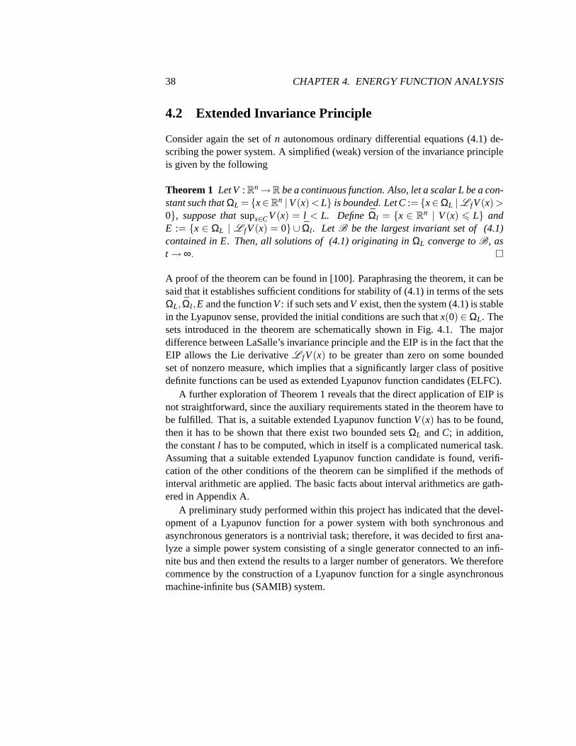
38 CHAPTER 4. ENERGY FUNCTION ANALYSIS
4.2 Extended Invariance Principle
Consider again the set ofn autonomous ordinary differential equations (4.1) de-scribing the power system. A simplified (weak) version of the invariance principleis given by the following
Theorem 1 Let V : Rn→R be a continuous function. Also, let a scalar L be a con-
stant such thatΩL = x∈Rn |V(x) < L is bounded. Let C:= x∈ΩL |L fV(x) >
0, suppose thatsupx∈CV(x) = l < L. DefineΩl = x ∈ Rn | V(x) 6 L and
E := x ∈ ΩL | L fV(x) = 0 ∪ Ωl . Let B be the largest invariant set of (4.1)contained in E. Then, all solutions of (4.1) originating inΩL converge toB, ast→ ∞.
A proof of the theorem can be found in [100]. Paraphrasing the theorem, it can besaid that it establishes sufficient conditions for stability of (4.1) in terms of thesetsΩL,Ωl ,E and the functionV: if such sets andV exist, then the system (4.1) is stablein the Lyapunov sense, provided the initial conditions are such thatx(0) ∈ΩL. Thesets introduced in the theorem are schematically shown in Fig. 4.1. The majordifference between LaSalle’s invariance principle and the EIP is in the fact that theEIP allows the Lie derivativeL fV(x) to be greater than zero on some boundedset of nonzero measure, which implies that a significantly larger class of positivedefinite functions can be used as extended Lyapunov function candidates (ELFC).
A further exploration of Theorem 1 reveals that the direct application of EIP isnot straightforward, since the auxiliary requirements stated in the theorem have tobe fulfilled. That is, a suitable extended Lyapunov functionV(x) has to be found,then it has to be shown that there exist two bounded setsΩL andC; in addition,the constantl has to be computed, which in itself is a complicated numerical task.Assuming that a suitable extended Lyapunov function candidate is found, verifi-cation of the other conditions of the theorem can be simplified if the methods ofinterval arithmetic are applied. The basic facts about interval arithmetics aregath-ered in Appendix A.
A preliminary study performed within this project has indicated that the devel-opment of a Lyapunov function for a power system with both synchronous andasynchronous generators is a nontrivial task; therefore, it was decided to first ana-lyze a simple power system consisting of a single generator connected to an infi-nite bus and then extend the results to a larger number of generators. We thereforecommence by the construction of a Lyapunov function for a single asynchronousmachine-infinite bus (SAMIB) system.
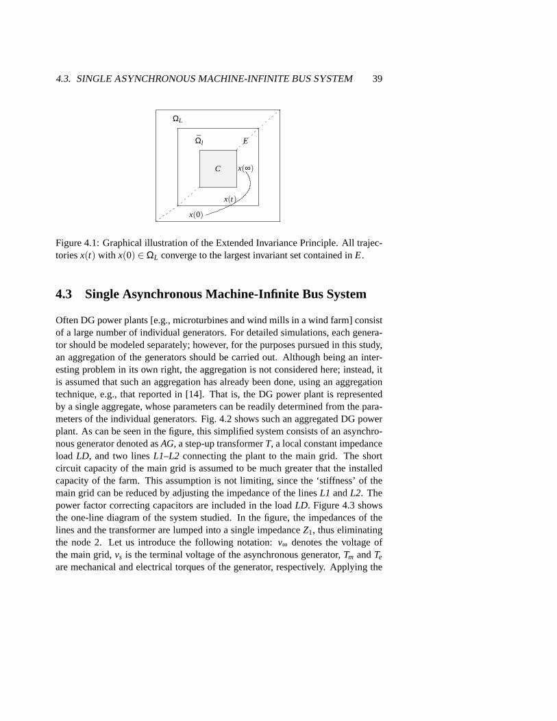
4.3. SINGLE ASYNCHRONOUS MACHINE-INFINITE BUS SYSTEM 39
C
ΩL
Ωl E
x(t)
x(0)
x(∞)
Figure 4.1: Graphical illustration of the Extended Invariance Principle. Alltrajec-toriesx(t) with x(0) ∈ΩL converge to the largest invariant set contained inE.
4.3 Single Asynchronous Machine-Infinite Bus System
Often DG power plants [e.g., microturbines and wind mills in a wind farm] consistof a large number of individual generators. For detailed simulations, eachgenera-tor should be modeled separately; however, for the purposes pursuedin this study,an aggregation of the generators should be carried out. Although being an inter-esting problem in its own right, the aggregation is not considered here; instead, itis assumed that such an aggregation has already been done, using an aggregationtechnique, e.g., that reported in [14]. That is, the DG power plant is representedby a single aggregate, whose parameters can be readily determined from the para-meters of the individual generators. Fig. 4.2 shows such an aggregatedDG powerplant. As can be seen in the figure, this simplified system consists of an asynchro-nous generator denoted asAG, a step-up transformerT, a local constant impedanceload LD, and two linesL1–L2 connecting the plant to the main grid. The shortcircuit capacity of the main grid is assumed to be much greater that the installedcapacity of the farm. This assumption is not limiting, since the ‘stiffness’ of themain grid can be reduced by adjusting the impedance of the linesL1 andL2. Thepower factor correcting capacitors are included in the loadLD. Figure 4.3 showsthe one-line diagram of the system studied. In the figure, the impedances ofthelines and the transformer are lumped into a single impedanceZ1, thus eliminatingthe node 2. Let us introduce the following notation:v∞ denotes the voltage ofthe main grid,vs is the terminal voltage of the asynchronous generator,Tm andTe
are mechanical and electrical torques of the generator, respectively.Applying the
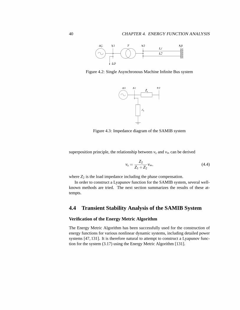
40 CHAPTER 4. ENERGY FUNCTION ANALYSIS Figure 4.2: Single Asynchronous Machine Infinite Bus system
Figure 4.3: Impedance diagram of the SAMIB system
superposition principle, the relationship betweenvs andv∞ can be derived
vs =Z2
Z1 +Z2v∞, (4.4)
whereZ2 is the load impedance including the phase compensation.In order to construct a Lyapunov function for the SAMIB system, several well-
known methods are tried. The next section summarizes the results of these at-tempts.
4.4 Transient Stability Analysis of the SAMIB System
Verification of the Energy Metric Algorithm
The Energy Metric Algorithm has been successfully used for the construction ofenergy functions for various nonlinear dynamic systems, including detailedpowersystems [47, 131]. It is therefore natural to attempt to construct a Lyapunov func-tion for the system (3.17) using the Energy Metric Algorithm [131].

4.4. TRANSIENT STABILITY ANALYSIS OF THE SAMIB SYSTEM 41
The main steps of the algorithm for constructing a Lyapunov function for (3.17)are outlined in Algorithm 1.Algorithm 1:
1. Eliminate the time variable from the differential equations describing thesystem
dξ1
dξ2=−a2ξ1 +x∗3ξ2 +x∗2ξ3 +ξ2ξ3
−a2ξ2−x∗3ξ1−x∗1ξ3−ξ1ξ3(4.5)
dξ2
dξ3=−a2ξ2−x∗3ξ1−x∗1ξ3−ξ1ξ3
c2vdsξ1 +c2vqsξ2(4.6)
dξ3
dξ1=
c2vdsξ1 +c2vqsξ2
−a2ξ1 +x∗3ξ2 +x∗2ξ3 +ξ2ξ3(4.7)
2. Convert the differential equations to 3 one-formsωi by multiplying andclearing the denominator terms.
3. Reduce the one-forms to a single one-formω(ξ ) by addition and substitutionof the 3 one-forms.
4. Perform line integration ofω(ξ ) along some path, which for simplicity canbe chosen along the ‘elbow’ path.
It appears however that no Lyapunov function can be constructed for the sys-tem (3.17) using the Energy Metric Algorithm. This result is summarized in thefollowing
Proposition 1 The model (3.17) admits no energy function constructed by Algo-rithm 1.
Proof Consider the line integral generated by Algorithm 1.
V =∫
Γ
a2c2vqsξ2 +a2c2vds(ξ1 +ξ2)+c2vds(ξ1 +x∗1)ξ3
+ c2vdsξ1x∗3 dξ1 +c2vds(ξ1 +ξ2 +x∗2)ξ3
+ c2vds(ξ1 +ξ2)x∗3 +c2vqsξ2(ξ3 +x∗3)
+ a2c2vqsξ2
dξ2 +
a22(ξ1 +ξ2)+a2ξ1x∗3
+ a2(ξ1 +x∗1−x∗2)ξ3 +(ξ1 +x∗1)ξ3(ξ3 +x∗3)
+ ξ1x∗3(ξ3 +x∗3)dξ3, (4.8)
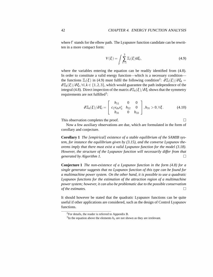
42 CHAPTER 4. ENERGY FUNCTION ANALYSIS
whereΓ stands for the elbow path. The Lyapunov function candidate can be rewrit-ten in a more compact form:
V(ξ ) =∫
Γ
3
∑i=1
Ξi(ξ )dξi , (4.9)
where the variables entering the equation can be readily identified from (4.8).In order to constitute a valid energy function—which is a necessary condition—the functionsΞi(ξ ) in (4.9) must fulfil the following condition2: ∂Ξi(ξ )/∂ξk =∂Ξk(ξ )/∂ξi ,∀i,k∈ 1,2,3, which would guarantee the path independence of theintegral (4.8). Direct inspection of the matrix∂Ξk(ξ )/∂ξi shows that the symmetryrequirements are not fulfilled3:
∂Ξk(ξ )/∂ξi =
h11 0 0c2vdsx∗3 h22 0
h31 0 h33
,h31 > 0,∀ξ . (4.10)
This observation completes the proof. Now a few auxiliary observations are due, which are formulated in the formof
corollary and conjecture.
Corollary 1 The [empirical] existence of a stable equilibrium of the SAMIB sys-tem, for instance the equilibrium given by (3.15), and the converse Lyapunov the-orems imply that there must exist a valid Lyapunov function for the model (3.18).However, the structure of the Lyapunov function will necessarily differ from thatgenerated by Algorithm 1.
Conjecture 1 The non-existence of a Lyapunov function in the form (4.8) for asingle generator suggests that no Lyapunov function of this type can be found fora multimachine power system. On the other hand, it is possible to use a quadraticLyapunov functions for the estimation of the attraction region of a multimachinepower system; however, it can also be problematic due to the possible conservatismof the estimates.
It should however be stated that the quadratic Lyapunov functions can be quiteuseful if other applications are considered, such as the design of Control Lyapunovfunctions.
2For details, the reader is referred to Appendix B.3In the equation above the elementshii are not shown as they are irrelevant.

4.4. TRANSIENT STABILITY ANALYSIS OF THE SAMIB SYSTEM 43
Verification of the First Integral of Motion Algorithm
The first integral of motion has been successfully used in power system applica-tions for generating Lyapunov functions [95]. To facilitate the presentation, theessential steps of the construction of a Lyapunov function using this technique arehighlighted in the followingAlgorithm 2:
1. Define the quantity dt as is shown below
dt =dξ1
−a2ξ1 +x∗3ξ2 +x∗2ξ3 +ξ2ξ3(4.11)
=dξ2
−a2ξ2−x∗3ξ1−x∗1ξ3−ξ1ξ3(4.12)
=dξ3
c2vdsξ1 +c2vqsξ2(4.13)
2. Perform line integration of the separate pairs (4.11)–(4.13) along the sys-tem’s post-fault trajectory.
3. Identify the energy function as the function obtained in the previous step.
Let us now show that Algorithm 2 cannot be applied to generate a Lyapunov func-tion for (3.17).
Proposition 2 The model (3.17) admits no Lyapunov function constructed by Al-gorithm 2.
Proof The necessary and sufficient condition for the existence of a Lyapunovfunction generated by Algorithm 2 is the following equality
Trace∇(Aξ +g) = 0, (4.14)
where∇ denotes the gradient of the vector fieldAξ +g. As can be easily verified,in the present case the equality (4.14) does not hold.
Verification of Krasovskii’s method for the SAMIB system
Another well-known method for the construction of Lyapunov functions is dueto Krasovskii [68]. The mathematical machinery of Krasovskii’s method is fairlysimple and is summarized in the following theorem [19]:
44 CHAPTER 4. ENERGY FUNCTION ANALYSIS
Theorem 2 Let f(ξ ) be differentiable w.r.t.ξ and let f(0) = 0; then the originis: (a) stable if the matrix H= ∂ f ′/∂ξ +∂ f/∂ξ ′ is negative semidefinite in someneighborhoodN of the origin, (b) asymptotically stable if H is negative definitein N , or (c) asymptotically stable in the large if H is negative definite for allξand f′ f is radially unbounded.
Let us now show that Krasovskii’s method fails to yield a Lyapunov functionforthe SAMIB system. This statement is formulated in the following
Proposition 3 The model (3.17) admits no Lyapunov function constructed by themethod of Krasovskii.
Proof Clearly, the conditions of Theorem 2 are fulfilled for the system (3.17),i.e.,(Aξ +g(ξ ))(0) = 0 and(Aξ +g(ξ )) is continuously differentiable in the entirestate space. Moreover, the function‖(Aξ +g(ξ ))‖22 = (Aξ +g(ξ ))′(Aξ +g(ξ )) isradially unbounded, i.e., lim‖ξ‖→∞ ‖(Aξ +g(ξ ))‖22 = ∞.
Let us now determine the sign definiteness of the matrixH. Omitting the alge-bra, this matrix can be written in the following form
H =
−2a2 0 c2vds+ξ2 +x∗20 −2a2 c2vqs−ξ1−x∗1
c2vds+ξ2 +x∗2 c2vqs−ξ1−x∗1 0
The application of Sylvester’s criterion indicates thatH in this particular case isnegative definite if and only if its determinant is negative. However, the determi-nant is nonnegative for allξ ∈ R
3, as (4.15) shows.
|H|= 2a2((c2vds+ξ2 +x∗2)2 +(c2vqs−ξ1−x∗1)
2) (4.15)
Therefore,H is sign indefinite, which implies thatf ′ f does not qualify as a validLyapunov function. This concludes the proof.
The Existence of a Quadratic Lyapunov Function
As was already stated in Corollary 1, for any dynamic system [with differentiablevector field] possessing a stable equilibrium there exists an appropriate Lyapunovfunction in some neighborhood of the equilibrium.
A naıve reasoning of this statement applied to the present system (3.17) mayinclude the following line of argumentation. Since the vector field(Aξ +g) in our

4.5. ALTERNATIVE FORMULATION OF THE SYSTEM MODEL 45
case can be directly decomposed into a linear and nonlinear part, and the 2-normof the nonlinear part vanishes as‖ξ‖2 approaches the origin, i.e.,
lim‖ξ‖2→0
‖g(ξ )‖2/‖ξ‖2 = 0,
in some neighborhoodN of the equilibrium the dynamics of the linear part willdominate those of the nonlinear part4. Therefore, the stability of the equilibriumwill be solely determined by the eigenvalues of the matrixA,∀ξ ∈N . Therefore, ifall the eigenvalues have strictly negative real parts, there should exist an appropri-ate quadratic Lyapunov function which can be found by solving the correspondingmatrix Lyapunov equation or determined as in the example on page 36. It is how-ever known, that in practical applications such quadratic Lyapunov functions yieldoverly conservative estimates of the associated attraction domain; therefore, theapplication of quadratic Lyapunov functions will not be pursued in this thesis. In-stead, the system model will be reformulated in order to facilitate the constructionof an appropriate Extended Lyapunov function.
4.5 Alternative Formulation of the System Model
Let us reformulate the model (3.13) in order to obtain an alternative representationof the asynchronous generator in the polar coordinates(E,δ ):
E =xm
xrr
√
ψ2dr +ψ2
qr
δ = tan−1(−ψqr/ψdr). (4.16)
Then assuming for simplicity that the rotor voltages are zero and definingT0 =xrr /(ωsrr), X′ = xss−x2
m/xrr the model (3.13) transforms to the following systemof equations
dδdt
= ωr −ωs−Xs−X′
X′T0Evssin(δ +φ) (4.17)
dωr
dt= −
EX′M
vssin(δ +φ)+Tm
M(4.18)
dEdt
= −Xs
X′T0E +
Xs−X′
X′T0vscos(δ +φ). (4.19)
4In most practical cases (i.e.,f ∈C1) this decomposition can also be done as follows:f (x) :=(∂ f ′/∂x)x+ f (x)− (∂ f ′/∂x)x= Ax+g(x).

46 CHAPTER 4. ENERGY FUNCTION ANALYSIS
E
6jX ′
vs
Figure 4.4: Equivalent circuit of the model (4.20)–(4.22)
In equations (4.17)–(4.19) it was assumed thatvqs = vscosφ andvds = vssinφ ,wherevs and φ are the magnitude and phase angle of the stator voltage ¯vs. Tosimplify the notation, let us denoteω = ωr −ωs and introduce the following con-stants: η1 = Xs/(X′T0),η2 = vs(Xs− X′)/(X′T0),θ = δ + φ , η3 = Tm/M, andη4 = vs/(X′M). To make the model more realistic, a damping termD = Tf /Mproportional to the friction torqueTf is added to (4.18), resulting in the followingmodel
dθdt
= ω−η2
Esinθ (4.20)
dωdt
= η3−η4Esinθ −Dω (4.21)
dEdt
= −η1E +η2cosθ . (4.22)
It can be noticed that the model given by the equations (4.20)–(4.22) to a certaindegree resembles the equations describing a single machine system with flux decaymodel; however, the physical meaning of the state variables of these two models isquite different [95]. Figure 4.4 shows the equivalent circuit of the model.
Construction of the Lyapunov function for the simplified SAMI Bsystem
Construction of a suitable Lyapunov function or Extended Lyapunov function forthe system (4.20)–(4.22) has proven a very challenging mathematical task,whichconfirmed the main conclusions from Section 4.4. Therefore, it was decided tofurther reduce the order of the model. To do so, we postulate that
η−11 E→ 0, (4.23)

4.5. ALTERNATIVE FORMULATION OF THE SYSTEM MODEL 47
which rendersE an algebraic variable. This approximation can be justified by thefollowing argument.
Consider again the differential equation describing the time evolution ofE, i.e.,(4.22). Let us now solve the equation, assuming thatθ is an unknown function oftime. The solution is given by the expression
E(t) = E0exp(−η1t)+exp(−η1t)η2
∫ t
0exp(η1τ)cosθ (τ)dτ. (4.24)
Taking the absolute value of both sides of (4.24) and noting that exp(η1τ)cosθ (τ)is dominated by exp(η1τ), the following inequality can be obtained
|E(t)|6 E0exp(−η1t)+exp(−η1t)η2
∣∣∣∣
∫ t
0exp(η1τ)dτ
∣∣∣∣. (4.25)
Evaluating the integral in (4.25), the estimate ofE(t) reduces to
|E(t)|6 E0exp(−η1t)+η2
η1(1−exp(−η1t)) . (4.26)
Clearly, for large values ofη1, the internal voltageE(t) is mainly determined bythe quotientη2/η1. According to [106], for the typical parameter values of windturbines in the range 500kW to 1MW, the values ofη1 are in the range[11.1,28.9].Recalling thatη2 is linearly proportional to the terminal voltage of the asynchro-nous generator, we conclude that variationsE(t) follow closely the variations inthe terminal voltage.
Thus, assuming
E =η2
η1cosθ ,
we arrive at the following second-order model:
θ = ω−η1 tanθ (4.27)
ω = η3−η2η4
2η1sin(2θ)−Dω . (4.28)
Consider the following new energy function candidate obtained by numeroustrial-and-error experiments
V(θ ,ω) =ω2
2−η3θ −
η2η4
4η1cos(2θ)+V0, (4.29)

48 CHAPTER 4. ENERGY FUNCTION ANALYSIS
whereV0 is an arbitrary constant. In some neighborhood of(θ0,ω0), the functionV is locally positive definite. The Lie derivative ofV along the planar vector field(4.27)–(4.28) is given by the expression
L fV(θ ,ω) = η1η3 tanθ −η2η4sin2 θ −Dω2. (4.30)
The functionL fV suggests that there are sets in theδ −ω plane where the Liederivative is positive; the boundedness of these sets needs to be checked, in orderto verify that (4.29) fulfills the conditions of Theorem 1, i.e., that it is an ExtendedLyapunov function. We will use interval arithmetics to numerically perform theverification.
Construction of the Lyapunov function for the full SAMIB syst em
Let us now relax the assumption (4.23) and derive a new energy functionfor the fullmodel (4.20)–(4.22) and consider the following new Lyapunov function candidate
V(θ ,ω ,E) =η2
2η4ω2−
η2η3
η4θ −η2Ecosθ +
η1
2E2 +V0. (4.31)
The Lie derivative of (4.31) is given by
L fV(θ ,ω ,E) =−η2Dη4
ω2−η22 sin2 θ +
η22η3
η4Esinθ − E2. (4.32)
Direct inspection of (4.32) reveals that large deviations ofE from the equilibriumpoint can result in positiveL fV. This observation would severely affect the useof conventional energy function methods; however, it is less restrictivefor the Ex-tended Invariance Principle. Technically, it is only necessary to assurethat the set(θ ,ω ,E) ∈ R
3 : L fV > 0 is bounded. Apparently,L fV is finite in the wholestate space, except for the manifold(θ ,ω ,0)5. For obvious reasons, it is also de-sirable to ensure that the set on whichL fV > 0 is as small as possible. As before,the properties ofL fV should be checked numerically.
Construction of the Lyapunov function for the three-bus power system
The construction of the energy function for the three-machine power system pre-sented in this subsection is based on the so-called “State Function Method” [108].
5On the manifoldE = 0, the function (4.31) is not analytic; however, the model of asynchronousgenerator itself is invalid on this manifold. Therefore, the state spaceU of the generator should berestricted such thatE = 0 is excluded from it.

4.5. ALTERNATIVE FORMULATION OF THE SYSTEM MODEL 49
G1
G2
G3
Passivenetwork
?
?
?
LD1
LD2
LDn
Figure 4.5: Simple three-machine power system.
The development of the energy function is mainly due to [60]; however, theanaly-sis and interpretation of the energy function are made by the author and arenovel.
The simple multimachine power system consists of two synchronous machines(a generator and a motor) and one asynchronous generator, which are schematicallyshown in Fig. 4.5. The electrical machines are interconnected in the passive net-work whose transfer conductances are assumed to be negligibly small. Themodelof the asynchronous generator is slightly changed in order to conform tothe modelof a synchronous generator. That is, equation (4.20) is differentiatedw.r.t timeand equation (4.21) is substituted into it, which is followed by shifting the stableequilibrium of the three-machine system to the origin. More details can be foundin [60]. Thus, the power system is modeled by the following set of equations:
M1x1 = −D1x1−E1B12[(Eo2 +x4)sin(x12+δ o
12)−Eo2 sinδ o
12]
+ E1E3B13[sin(x13+δ o13)−sinδ o
13] (4.33)
M2x2 = −K1(x)x1− (D2 +K1(x)+K3(x))x2−K3(x)x3−K4(x)x4
− E1B12[(Eo2 +x4)sin(x12+δ o
12)−Eo2 sinδ o
12]
+ E3B23[(Eo2 +x4)sin(x23+δ o
23)−Eo2 sinδ o
23] (4.34)
M3x3 = −D3x3−E1E3B13[sin(x13+δ o13)−sinδ o
13]
− E3B23[(Eo2 +x4)sin(x23+δ o
23)−Eo2 sinδ o
23] (4.35)
x4 = T−12 (1−xmB22)x4 +KaM−1
2 [cosδ o12−cos(x12+δ o
12)]
+ KbM−12 [cosδ o
23−cos(x23+δ o23)], (4.36)
50 CHAPTER 4. ENERGY FUNCTION ANALYSIS
where the statesxik are defined asxi − xk. Mi andDi are the inertia constant andthe damping of machinei, respectively.Ek andT2 denote the transient EMF ofmachinek and the ‘open circuit time constant’ of the asynchronous generator;Bik
is the (i,k)’s element of the reduced network matrix of the power system. ThefunctionsKa, Kb, andK1, . . . ,K4 are defined as follows.
Ka =xm
T2B12E1M2
Kb =xm
T2B23E3M2
K1(x) = Kacos(x12+δ 0
12)
x4 +E02
(4.37)
K3(x) = Kbcos(x23+δ 0
23)
x4 +E02
(4.38)
K4(x) = −Kasin(x12+δ 0
12)
(x4 +E02)2
+Kbsin(x23+δ 0
23)
(x4 +E02)2
. (4.39)
In the equations above, the state variables with superscript ‘0’ denote thesteadystate values of the corresponding state.
Defining the new constant matricesM,Ms,C,Cs,Dc, the variable matrixDv, thenew variablesσ , and the vector-valued functionf (σ) as follows,
Ms = diag(M1,M2,M3), M = diag(Ms,1), Dc = diag(D1,D2,D3,1)
Cs =
1 −1 01 0 −10 1 −1
, C =
[Cs 00 1
]
, A =
[I3 00 0
]
, σ = Cx,
Dv =
0 0 0 0−K1(x) K1(x)+K3(x) −K3(x) −K4(x)
0 0 0 00 0 0 0
f (σ) =
E1B12[(E02 +x4)sin(σ1 +δ 0
12)−E02 sinδ 0
12]E1E3B13[sin(σ2 +δ 0
13)−sinδ 013]
E3B23[(E02 +x4)sin(σ3 +δ 0
23)−E02 sinδ 0
23]f5(σ)
f5(σ) = T−12 (1−xmB22)σ4 +KaM−1
2 [cosδ 012−cos(σ1 +δ 0
12)]
+ KbM−12 [cosδ 0
23−cos(σ3 +δ 023)],

4.5. ALTERNATIVE FORMULATION OF THE SYSTEM MODEL 51
equations (4.33)–(4.36) can be put in matrix form:
Ax+M−1(Dc +Dv)x+M−1C′ f (σ) = 0. (4.40)
The energy function is sought in the following form:
V(x, x) =∫ x
0QAxdx+
∫ x
0QM−1C′ f (Cx)dx. (4.41)
The unknown nonsingular matrixQ is the main design parameter which has to bedetermined. The key idea is to find such a matrixQ that the function (4.41) satisfiesthe associated curl equations and the Rayleigh dissipation function ˙x′(QM−1(Dc +Dv))x > 0, which will ensure that the line integrals in (4.41) are path independentand the Lie derivative ofV is non-positive definite.
It is shown in [60] that for somem > 0, l > −m/Trace(MS), the matrixQdefined as
Q =
[mMs+ lMs1Ms 0
0 mT2/xm
]
satisfies the curl equations associated withV. Thus, the following energy functionis obtained
V(x, x) =12
x′+ [mM1 + lM11M1] x+
+ m [E1B12(E02 +σ4)cosδ 0
12−cos(σ1 +δ 012)−σ1E0
2 sinδ 012
+ E1E3B13cosδ 013−cos(σ2 +δ 0
13)−σ2sinδ 012
+ E3B23(E02 +σ4)cosδ 0
23−cos(σ3 +δ 023)−σ3E0
2 sinδ 023
+ (2xm)−1(1−xmB22)σ24 ], (4.42)
wherex+ = [x1,x2,x3]′. It can be shown that the Lie derivative of (4.42) is given
by the expression:
L fV(x, x) = −12
x′+(QM−1(Dc +Dv)+(Dc +Dv)′M−1Q)x+
= −12
x′+(QM−1Dc +D′cM−1Q)x+
−12
x+(QM−1Dv +D′vM−1Q)x+
= −12
x′+Rcx+−12
x′+Rv(x)x+. (4.43)

52 CHAPTER 4. ENERGY FUNCTION ANALYSIS
In order to apply (4.43) for stability studies, its properties should be clarified. Inparticular, the sign definiteness ofL fV should be determined, which can be doneby a closer examination of matricesRc andRv(x). Clearly,Rc < 0, which howeverdoes not guarantee thatL fV is non-positive. In [60], it was assumed thatE2(t)could be linearized around the post-fault equilibrium and conditions were derivedwhich would assure positive definiteness ofRc +Rv. However, it should be notedthat the assumption on small changes inE2(t) might be unrealistic, sinceE2(t)heavily depends on the terminal voltage of the asynchronous generator;should theterminal voltage change,E2(t) will also change in fractions of a second.
Let us denote the maximum and the minimum eigenvalue ofRc andRv(x) byλmax andλmin, respectively
λmax = maxλ (Rc)= 2m max(D1,D2,D3,T2x−1m (4.44)
λmin = minλ (Rv(x))= 2m (K1(x)+K3(x)). (4.45)
It is important to note that bothλmin and λmax depend linearly on the arbitraryconstantm, implying that both equalities (4.44) and (4.45) hold for any choice ofm. Therefore, in general, the negative definiteness ofL fV in (4.43) cannot beascertained by the choice ofm.
Recalling the inequalities from Appendix B,
x′Rcx 6 λmax‖x‖2
x′Rv(x)x > λmin‖x‖2,
the best and the worst-case scenarios can be considered:
Best caseThe system dynamics evolve in the [nonempty] null spaceNRv = kerRv
of the matrixRv, or alternativelyλmax+ λmin > 0 ∀x. Then, the time deriv-ative ofV is at least nonpositive, which guarantees that(Rc +Rv) < 0, thusrenderingV a valid energy function.
Worst case If ∃ [τ1,τ2] : (Rc + Rv)(τ) ≺ 0 for all τ ∈ [τ1,τ2] and τ1 6= τ2, thenL fV(τ) > 0, which invalidates the energy function candidateV given byexpression (4.42).
Obviously, the realization of either the best or the worst case scenarios cannot beasserted without running a time domain simulation, which makes the direct use ofV questionable. However, in the framework of the Extended Invariance Principle,V can constitute a valid extended Lyapunov function if the conditions of Theorem 1
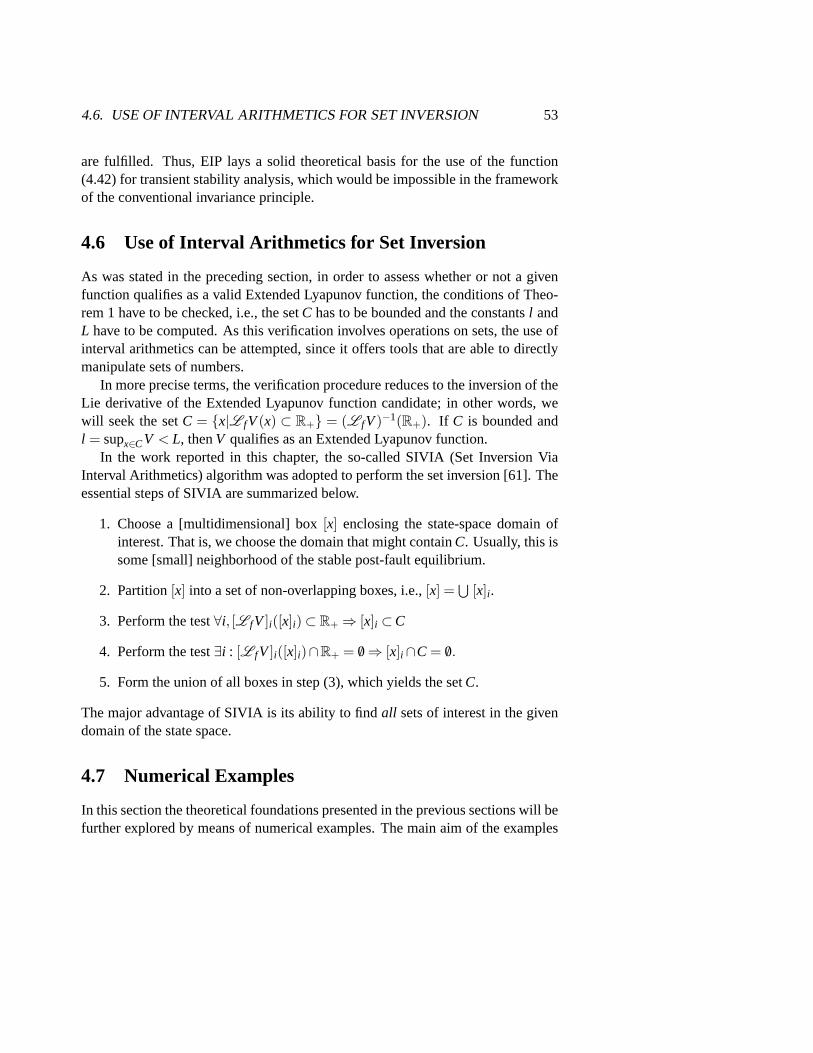
4.6. USE OF INTERVAL ARITHMETICS FOR SET INVERSION 53
are fulfilled. Thus, EIP lays a solid theoretical basis for the use of the function(4.42) for transient stability analysis, which would be impossible in the frameworkof the conventional invariance principle.
4.6 Use of Interval Arithmetics for Set Inversion
As was stated in the preceding section, in order to assess whether or not agivenfunction qualifies as a valid Extended Lyapunov function, the conditions ofTheo-rem 1 have to be checked, i.e., the setC has to be bounded and the constantsl andL have to be computed. As this verification involves operations on sets, the useofinterval arithmetics can be attempted, since it offers tools that are able to directlymanipulate sets of numbers.
In more precise terms, the verification procedure reduces to the inversionof theLie derivative of the Extended Lyapunov function candidate; in other words, wewill seek the setC = x|L fV(x) ⊂ R+ = (L fV)−1(R+). If C is bounded andl = supx∈CV < L, thenV qualifies as an Extended Lyapunov function.
In the work reported in this chapter, the so-called SIVIA (Set InversionViaInterval Arithmetics) algorithm was adopted to perform the set inversion [61]. Theessential steps of SIVIA are summarized below.
1. Choose a [multidimensional] box[x] enclosing the state-space domain ofinterest. That is, we choose the domain that might containC. Usually, this issome [small] neighborhood of the stable post-fault equilibrium.
2. Partition[x] into a set of non-overlapping boxes, i.e.,[x] =⋃
[x]i .
3. Perform the test∀i, [L fV]i([x]i)⊂ R+⇒ [x]i ⊂C
4. Perform the test∃i : [L fV]i([x]i)∩R+ = /0⇒ [x]i ∩C = /0.
5. Form the union of all boxes in step (3), which yields the setC.
The major advantage of SIVIA is its ability to findall sets of interest in the givendomain of the state space.
4.7 Numerical Examples
In this section the theoretical foundations presented in the previous sections will befurther explored by means of numerical examples. The main aim of the examples
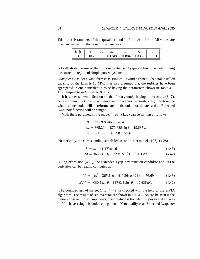
54 CHAPTER 4. ENERGY FUNCTION ANALYSIS
Table 4.1: Parameters of the equivalent model of the wind farm. All values aregiven in per unit on the base of the generator
H, [s] rr rs xs xr xm vs
4 0.0073 0 0.1248 0.0884 1.8365 0+ j1
is to illustrate the use of the proposed extended Lyapunov functions determiningthe attraction region of simple power systems.
Example:Consider a wind farm consisting of 10 wind turbines. The total installedcapacity of the farm is 10 MW. It is also assumed that the turbines have beenaggregated in one equivalent turbine having the parameters shown in Table 4.1.The damping termD is set to 0.05 p.u.
It has been shown in Section 4.4 that for any model having the structure (3.17),certain commonly known Lyapunov functions cannot be constructed; therefore, thewind turbine model will be reformulated in the polar coordinates and an ExtendedLyapunov function will be sought.
With these parameters, the model (4.20)–(4.22) can be written as follows
θ = ω−9.9816E−1sinθω = 365.21−1877.68Esinθ −19.635ωE = −11.173E +9.9816cosθ
Numerically, the corresponding simplified second-order model (4.27)–(4.28) is
θ = ω−11.173tanθ (4.46)
ω = 365.21−838.729sin(2θ)−19.635ω . (4.47)
Using expression (4.29), the Extended Lyapunov function candidate and its Liederivative can be readily computed as
V =12
ω2−365.21θ −419.36cos(2θ)+456.69 (4.48)
L fV = 4080.5tanθ −18742.3sin2 θ −19.635ω2. (4.49)
The boundedness of the setC for (4.49) is checked with the help of the SIVIAalgorithm. The results of set inversion are shown in Fig. 4.6. As can be seen in thefigure,C has multiple components, one of which is bounded. In practice, it sufficesfor V to have a single bounded component ofC to qualify as an Extended Lyapunov
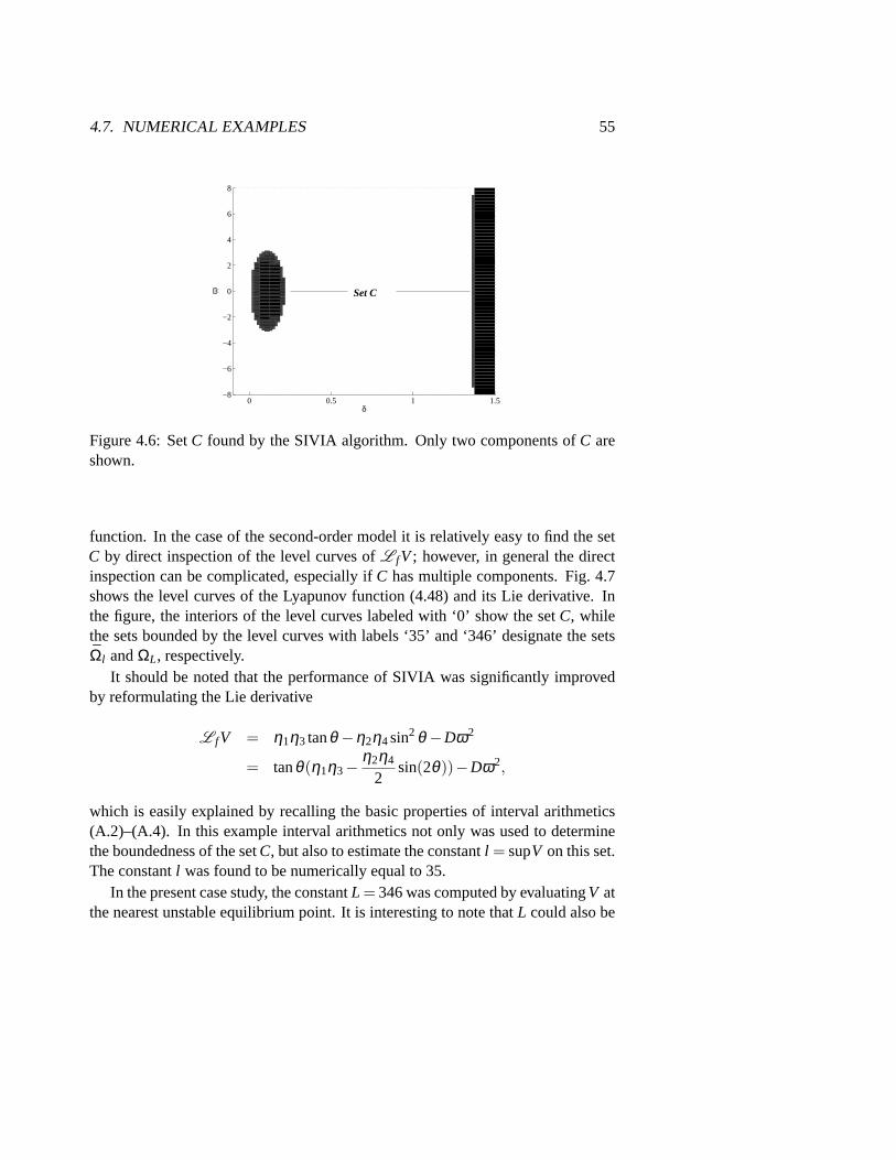
4.7. NUMERICAL EXAMPLES 55
0 0.5 1 1.5−8
−6
−4
−2
0
2
4
6
8
δ
ω Set C
Figure 4.6: SetC found by the SIVIA algorithm. Only two components ofC areshown.
function. In the case of the second-order model it is relatively easy to find the setC by direct inspection of the level curves ofL fV; however, in general the directinspection can be complicated, especially ifC has multiple components. Fig. 4.7shows the level curves of the Lyapunov function (4.48) and its Lie derivative. Inthe figure, the interiors of the level curves labeled with ‘0’ show the setC, whilethe sets bounded by the level curves with labels ‘35’ and ‘346’ designatethe setsΩl andΩL, respectively.
It should be noted that the performance of SIVIA was significantly improvedby reformulating the Lie derivative
L fV = η1η3 tanθ −η2η4sin2 θ −Dω2
= tanθ(η1η3−η2η4
2sin(2θ))−Dω2,
which is easily explained by recalling the basic properties of interval arithmetics(A.2)–(A.4). In this example interval arithmetics not only was used to determinethe boundedness of the setC, but also to estimate the constantl = supV on this set.The constantl was found to be numerically equal to 35.
In the present case study, the constantL = 346 was computed by evaluatingV atthe nearest unstable equilibrium point. It is interesting to note thatL could also be

56 CHAPTER 4. ENERGY FUNCTION ANALYSIS
−2 −1.5 −1 −0.5 0 0.5 1 1.5 2−30
−20
−10
0
10
20
30
δ
ω
Level curves of V(δ,ω) and dV/dt(δ,ω)
0
0
0
0
0
0
0
0
0
0
0
0
0 35
35
35 346
346
346
346
346
346
ΩL
Ωl
C
Figure 4.7: Level curves ofV andL fV
Vp
t [s]0.2 0.4 0.6 0.8 1 1.2
50
100
150
200
250
300
350
Figure 4.8: Potential energy curve vs. time for the system (4.46)–(4.47).The poten-tial energy was computed for a hypothetic fault on the transmission system, whichresulted in a 60% voltage drop at the terminals of the asynchronous generator.

4.7. NUMERICAL EXAMPLES 57
Table 4.2: System parameters for 3-machine power system. All values are givenin per unit, exceptδ0 andT2. With minor modifications, the parameters values aresimilar the values in [60].
M D x′d E0 δ0[rad] xm T2 [s] slip(0)
G1 0.0132 0.0132 0.15 1.48 0.3 — — 0G2 0.004 0 0.137 1 0.2 2.15 0.235−0.0193G3 0.065 0.0325 0.15 1.05 0 — — 0
determined be applying the argument of the PEBS method with the potential energydefined asVp =−η3θ −η2η4/(4η1)(cos(2θ +2θ0)−cos(2θ0)), see Fig. 4.8.
Since the conditions of Theorem 1 are fulfilled, it can be concluded that thefunction (4.48) is an Extended Lyapunov function and all trajectories initiated inΩL will eventually converge to the largest invariant set contained in the union ofΩl andx∈ΩL : L fV = 0.
Example:Let us now consider the three-machine power system. The power systemconsists of one synchronous generatorG1, one asynchronous generatorG2, and asynchronous motorG3 which are interconnected by 3 power lines connected in astar. The one-line diagram of the power system is shown in Fig. 4.9. The parame-ters of the generators are shown in Table 4.2. The power lines have the followingreactances in per unit:Z1 = j0.2, Z2 = j0.1, andZ3 = j0.1. The synchronous fre-quency was set to 120π. In this example a bolted6 three-phase fault is applied tothe terminals ofG3 which is then cleared. The main purpose of this example isto further explore and validate the extended Lyapunov function (4.42) and its Liederivative (4.43).
A series of nonlinear time-domain experiments were performed on the three-machine power system in MATLAB . Some of the results from the experimentswill be presently discussed. It is instructive to begin inspection of the numericalresults by observing the statex4 = E2−E2,0 and the phase portraits of the electricalmachines, see Fig. 4.10–4.14.
The simulations in this example confirm that the state variablex4 does devi-ate significantly from its steady state. For instance, in the present case under thefault, E2 reduced to approximately 25% of its steady state value, see Fig. 4.10.Physically, this is easily explained by the fact that the asynchronous generator doesnot have an excitation winding to supportE2 during the fault. Therefore,E2 can be
6To be exact, the fault reactance wasj10−5 p.u.

58 CHAPTER 4. ENERGY FUNCTION ANALYSIS
G1
G3
G2
Z1
Z3
Z2
Figure 4.9: Three-machine power system
0 1 2 3 4 5 6
−0.7
−0.6
−0.5
−0.4
−0.3
−0.2
−0.1
0
EMF ∆E2 vs time
Time [s]
∆ E
2 [pu]
Figure 4.10: The deviation of state variable,∆E2, i.e., the EMF of the asynchronousgenerator as a function of time
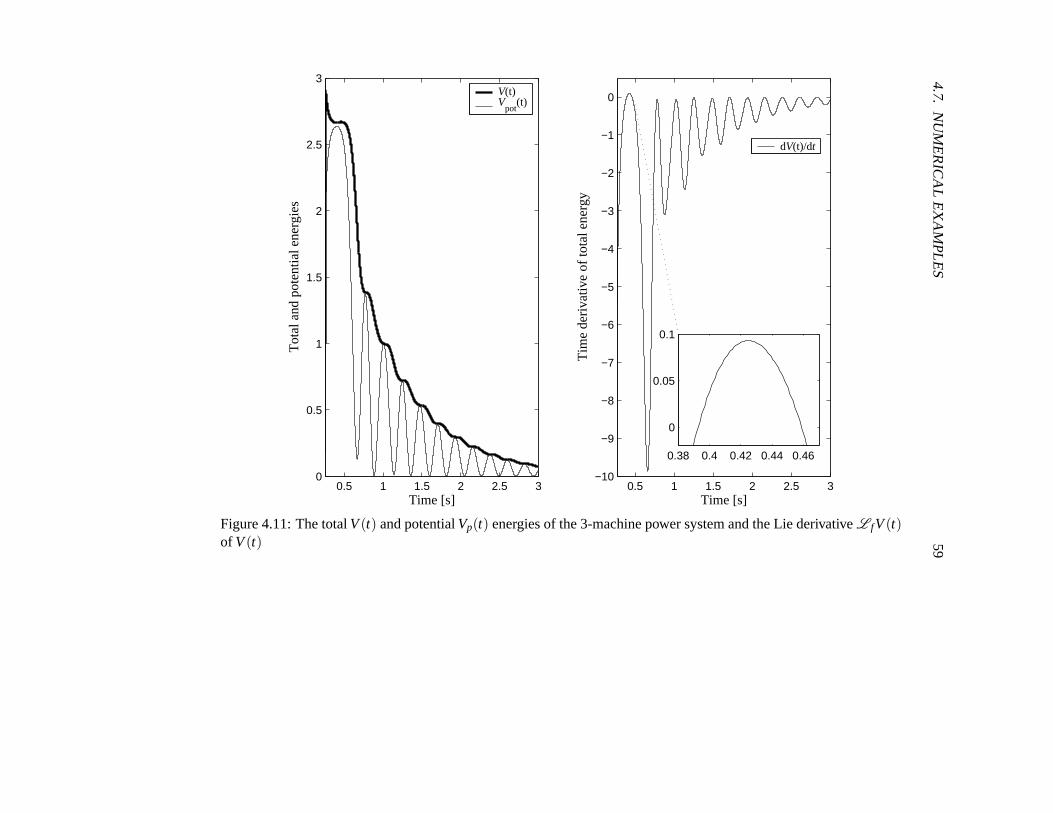
4.7.N
UM
ER
ICA
LE
XA
MP
LES
59
0.5 1 1.5 2 2.5 30
0.5
1
1.5
2
2.5
3
Time [s]
Tot
al a
nd p
oten
tial e
nerg
ies
0.5 1 1.5 2 2.5 3−10
−9
−8
−7
−6
−5
−4
−3
−2
−1
0
Time [s]
Tim
e de
rivat
ive
of to
tal e
nerg
y
0.38 0.4 0.42 0.44 0.46
0
0.05
0.1
dV(t)/dt
V(t)V
pot(t)
Figure 4.11: The totalV(t) and potentialVp(t) energies of the 3-machine power system and the Lie derivativeL fV(t)of V(t)

60 CHAPTER 4. ENERGY FUNCTION ANALYSIS
−0.4 −0.2 0 0.2 0.4 0.6 0.8 1 1.2 1.4 1.6
−10
−8
−6
−4
−2
0
2
4
6
8
10
G1 phase portrait. Case 1
δ1
ω1
Figure 4.12: Phase portrait ofG1
−0.3 −0.2 −0.1 0 0.1 0.2 0.3 0.4 0.5 0.6
−6
−5
−4
−3
−2
−1
0
1
2
3
4
G2 phase portrait. Case 1
δ2
ω2
Figure 4.13: Phase portrait ofG2

4.7. NUMERICAL EXAMPLES 61
−0.8 −0.6 −0.4 −0.2 0 0.2 0.4 0.6 0.8 1
−2
−1
0
1
2
3
G3 phase portrait. Case 2
δ3
ω3
Figure 4.14: Phase portrait ofG3
expected to fall rapidly as its terminal voltage decreases. This reduction in the mag-nitude ofE2 has an important implication – an increase of the absolute values of thevariablesKi(x)41, see (4.37)–(4.39). As a consequence,λmin in (4.45) increases inmagnitude, which in turn results in positiveL fV(x). Thus, strictly speaking, fromthe view point of the classical invariance principle, the positive definite function(4.42) is neither a Lyapunov nor an energy function, since the measure of the seton whichL fV > 0 is nonzero, as Fig. 4.11 shows. The conditions of Theorem 1were in this example verified numerically, using both interval arithmetics and theconventional real analysis.
A comparison of the critical clearing time computed by the step-by-step methodand the extended Lyapunov function, reveals that the estimates are not overly con-servative. For instance, for this example the step-by-step methods yieldstcc = 0.25s, while the Direct method suggeststcc = 0.241 s. That is, the error in the estimatein this case does not exceed 3.6%
62 CHAPTER 4. ENERGY FUNCTION ANALYSIS
4.8 Summary
This chapter reports preliminary results of a study concerned with the questionsrelated to the transient stability of power systems with asynchronous generators. Inthis study the asynchronous generators represent a large-scale windfarm consistingof fixed-speed wind turbines with fixed pitch. For a better understanding of thedynamic properties of the asynchronous generators, it is assumed that the necessaryturbine aggregation has been carried out and the farm can be readily representedby a single asynchronous machine connected to an infinite bus via a transmissionsystem.
The objective of the study was to develop a framework for studying the transientstability of the asynchronous generators similar to that of synchronous generators.That is, an attempt was made to apply a Lyapunov/energy function method to thesimple power system with an asynchronous generator.
Detailed analysis was performed in order to verify the existence of a properLyapunov function for the system at hand. It was demonstrated analytically thatthree commonly known method for construction Lyapunov functions cannotyielda Lyapunov function for the SAMIB system. Even though it does not imply that anappropriate Lyapunov function does not exist, it does indicate that the constructionof such a function might be a very difficult mathematical task. This fact suggeststhat other analytical tools should be be used for the stability studies of the powersystem with asynchronous generators.
The Extended Invariance Principle was found capable of constructing afunc-tion that could be used in the stability studies reported in this chapter. In particular,an extended Lyapunov function was found for a simple power system. Theuseof Extended Invariance Principle allows a larger class of functions to be appliedfor stability studies of power systems; however, this comes at the expense of hav-ing to perform certain operations on sets of reals. To overcome the difficulty ofmanipulating the sets, the utility of interval arithmetics is proposed.
Numerical examples are used to illustrate the application of Extended Invari-ance Principle and interval arithmetics for system stability analysis of a simplifiedmodel of a wind farm consisting of fixed-speed wind turbines and a model of athree-machine power system.

Part II
Voltage Stability
63


Chapter 5
Assessment of Voltage Stability ofUncertain Power Systems
“The actual science of logic is conversant at present only with things eithercertain, impossible, or entirely doubtful, none of which (fortunately) wehave to reason on. Therefore the true logic for this world is the calculusof Probabilities, which takes account of the magnitude of the probability
which is, or ought to be, in a reasonable man’s mind.”— James Clerk Maxwell (1850)
This chapter presents an application of interval arithmetics to voltage collapseanalysis. The problem of calculating the power system critical loading conditionsand determining the maximal loadability of a power system in a nondeterministicsetting are treated. The methodology for assessment of voltage stability in de-terministic power systems is well-established in the literature; however, voltagestability analysis of nondeterministic power systems has not yet received muchattention. In this chapter, the uncertain power system parameters such as, for in-stance, loads and partly controllable generation are treated as intervals and theanalysis is performed using the framework of interval arithmetics. The voltage sta-bility problem is restated in terms of an interval-valued optimization problem andis solved by applying the Generalized Newton method.
Numerical experiments are performed in order to demonstrate the technicalitiesof the proposed methodology. For the examples presented, the numerical results arefound to be reliable and nonconservative.
5.1 IntroductionReliable assessment of voltage stability of an electric power system is es-sential for its operation and control. To accommodate the need for accu-rate analysis of voltage stability a number of analytical and computational
tools have been developed [28], [58]. Typically, two voltage stability problems areanalyzed:
1. Determination of the maximum loadability problem and
65

66CHAPTER 5. ASSESSMENT OF VOLTAGE STABILITY OF UNCERTAIN
POWER SYSTEMS
2. Computation of the critical loading of the power system [67].
In the former case, a loading scenario is assumed and the maximum powertransfer to the load buses is computed. In the latter case, a minimum system loadingis sought that would render the power system voltage unstable, i.e., the loadingthat would cause voltage collapse. Such a loading is referred to as criticalsystemloading. From the standpoint of the system operator, the power system shouldbe controlled is such a way that the critical loading is prevented. A recent paperreported a new method for the assessment of voltage stability in power systemswith probabilistic nodal loading model [67].
It is shown in the literature that the voltage stability analysis problem can bereduced to a constrained optimization problem, see [28] and references therein.This consideration allows well-established techniques from optimization theorybeused in voltage stability analysis (VSA) studies. Typically, the direct optimizationof a certain objective function is performed, which yields the critical points whichare the solutions to either the maximum loadability or critical loading problem.Alternatively, the continuation method is used to solve the optimization problem[28], [67].
In all of the aforementioned publications, it is implicitly assumed that the powersystem is deterministic, with possibly one exception–the system loading which, insome cases, is assumed to be uncertain. While in some power systems this can-not be considered a problem, there are power systems which contain significantamounts of uncontrollable energy sources such as, for example, large wind farmsand for these power systems the uncertainty in power generation can be significant.As the voltage stability is—to a certain extent—a local problem, the uncertainty inthe power system parameters need to be explicitly accounted for. This chapterpresents a methodology for addressing the issue of uncertainty in the power sys-tem generation. The uncertain parameters of a power system are represented byintervals, i.e., it is explicitly assumed that although uncertain, the parameters arebounded. The VSA problem is reformulated in the form of an interval-valued op-timization and then solved using the methods of interval arithmetics.
5.2 Voltage Stability Formulation
System Modeling
In power systems analysis it is customary to model the network components withthe help of differential-algebraic equations which—in the general case—have the
5.2. VOLTAGE STABILITY FORMULATION 67
following form [28]
[x0
]
=
[f (t,x,y,λ , p)g(t,x,y,λ , p)
]
= F(z,λ , p). (5.1)
In equation (5.1), the vectorx ∈ Rn typically represents the state variables of the
various power system devices and their respective controls;y ∈ Rm is the vector
of algebraic variables which normally represent nodal voltages and angles of theload buses. Finally, the vectorsλ ∈R
l andp∈Rk stand for the set of slowly vary-
ing parameters e.g., system loading variations and the set of control parameters,respectively. It is assumed that the system operator does not have director controlover the parametersλ , as opposed to the parametersp which can directly or indi-rectly be altered by the operators. The vector-valued functionsf andg are definedas f : R×R
n×Rm×R
l ×Rk→ R
n andg : R×Rn×R
m×Rl ×R
k→ Rm. For
convenience, let us introduce the variablez= (x′,y′)′. Without significant loss ofgenerality, it is assumed in this chapter that the parametersp are kept constant andequal numerically to somep = po.
It is commonly assumed that the variablez evolves on such a manifoldM thatthe mappingDyg remains bijective for all time [54]. If this is the case, then thesystem (5.1) can be shown to have a unique solution and the algebraic equationscan be eliminated by means of the Implicit Function Theorem [104]. In this chapterit is assumed thatDyg∈M along all system trajectories.
Depending on the nature of the VSA studies, either the conventional power-flowequations or the complete set of differential-algebraic equations (5.1) areused inthe analysis and simulations. Nevertheless, as is reported in the literature, in manypractical cases the load-flow equations alone might be inappropriate for the needsof rigorous voltage stability analysis [29], [30].
Voltage Collapse
The operational principles of power systems are such that at an given timein-stant, the power system is subjected to the action of various perturbations. Forthe convenience of analysis, the perturbations can be subdivided into twocate-gories: slow and fast. All the systems considered in this chapter are assumed to beperturbed by slow variations in the parametersλ . As the parameter vectorλ al-ters, the equilibrium point(z∗,λ∗) of (5.1) moves in some domainΩ⊂R
n+m×Rl .
Upon approaching a local maximum of loading, the system (5.1) undergoesa localsaddle-node bifurcation, which is characterized by a unique zero eigenvalue of the
68CHAPTER 5. ASSESSMENT OF VOLTAGE STABILITY OF UNCERTAIN
POWER SYSTEMS
Jacobian matrixDx f (z∗,λ∗) and the transversality conditions
Dx f ·v = D′x f ·w′ = 0 (5.2)
w′Dλ f = 0 (5.3)
w′ ·D2x f ·v = 0. (5.4)
In equation (5.3), the variablesv andw stand for the normalized right and lefteigenvectors corresponding to the zero eigenvalue ofDx f . Note that the JacobiansDx f ,Dλ and HessianD2
x f in equations (5.2)–(5.4) are evaluated at the equilibrium(z∗,λ∗).
In order to ensure a reliable and proper operation of power systems, thecurrentequilibrium should not approach the local bifurcation point. Moreover, acertainvoltage stability margin should be identified [possibly based on practical experi-ence] and power system operated within this stability margin. On the other hand,because of certain economical and environmental considerations, many power sys-tems are presently operated in a proximity to their stability limits. Thus, it becomesan important task to reliably determine the local loadability limit for a given powersystem.
There exists a dual problem to the aforementioned one, namely, the determiningof the minimal load increase that causes a system bifurcation. This problem iscommonly referred to as ‘minimum distance to collapse.’
Both these problems can be reformulated as optimization problems in which theloadingλ is maximized and the distance‖λ −λo‖ is minimized, respectively. Thatis, the maximum loadability problem reduces to the optimization of the objectivefunction
minλ ,z
J1(λ ,z) =−λ (5.5)
s.t. F(z,λ ) = 0
while, the critical system loading can be computed by optimizing the followingobjective function
minλ ,z,w
J2(λ ,z,w) = ‖λ −λo‖2 (5.6)
s.t. (F(λ ,z)′,w′DzF(λ ,z))′ = 0.

5.3. APPLICATION OF INTERVAL ARITHMETICS TO VOLTAGECOLLAPSE ANALYSIS 69
Analytical Tools for VSA
Normally the constrained optimization problems (5.5)–(5.6) are solved either di-rectly by applying the Lagrange multipliers technique or using the so-called thecontinuation method. The direct method is less expensive numerically and onlyyields the set(λ∗,z∗,w∗). The latter technique is essentially based on repetitivecomputation of the system equilibria as the parameterλ (usually a scalar) is variedand thus is more expensive numerically, as compared to the direct method. Thedirect method is applied for all optimization tasks treated in this chapter.
In the discussion above, all the variables and parameters have been assumedknown exactly, which in certain situations might not be entirely true. For instance,in power systems with substantial penetration levels of distributed generation utiliz-ing uncontrollable energy sources, for instance wind energy, the power producedat a given time instant is not known in advance. On the other hand, the actualloading of a small power system also is to some extent uncertain. In large powersystems, the various loads are normally aggregated, which reduces the impact ofthe load uncertainty on the stability analysis. Nevertheless, the voltage instabilityphenomenon is considered to be a local one making a general discussion on thesuitability of aggregation of large loads a nontrivial task. It is therefore of interestto develop a VSA technique capable of accounting for uncertainties in the systemparameters. One of possible alternatives is to use intervals arithmetics to performthe constrained optimization tasks (5.5)–(5.6).
5.3 Application of Interval Arithmetics to VoltageCollapse Analysis
Let us reformulate the two constrained optimization problems (5.5)–(5.6) statedin Section 5.2 placing emphasis on the fact that some of the parameters are nowtreated as intervals. That is, now it is assumed that bothλ andz are uncertain, butbounded quantities. Then, the objective functionsJ1 andJ2 in (5.5)–(5.6) become
min[λ ],[z]
J1([λ ], [z]) =−[λ ] (5.7)
s.t.F([λ ], [z]) = 0
min[λ ],[z],[w]
J2([λ ], [z], [w]) = ‖[λ ]−λo‖2 (5.8)
s.t. (F([λ ], [z])′,w′DzF([λ ], [z]))′ = 0.
70CHAPTER 5. ASSESSMENT OF VOLTAGE STABILITY OF UNCERTAIN
POWER SYSTEMS
To solve either of (5.5) or (5.6), the method of Lagrange multipliers can be applied.A series of experiments was performed and it was observed that the so-called
naıve Newton method was able to yield acceptable results for the problems inwhich the interval parameters had relatively small uncertainties. To enhance thenumerical properties of the optimization, the Generalized Newton method (GN)was implemented, in which the Newton iterate is given by the expression [48]:
[uk+1] = uk∩ [uk−DuF−1(uk) ·F (uk)], (5.9)
where[uk] = [zk]× [λk]× [wk] andF is the Lagrangian defined as
F = ‖[λ ]−λo‖2 +s′1F([u])+s′2D′zF ·w, (5.10)
DuF stands for the gradient of the Lagrangian evaluated at[uk], ands1 and s2
are the respective Lagrange multipliers. The variablesu are treated as unknownintervals, the active powerP1 andP2 are assumed to be known intervals. All thecomputations are performed in MATLAB with the help of the package INTLAB[105].
Numerical Experiments
To exemplify the ideas presented in the preceding sections and facilitate the dis-cussion on the results obtained, a simple power system is chosen1. The powersystem consists of a slack node, three transmission lines, and twoPV nodes, seeFig. 5.1. The relevant parameters of the system are shown in the figure. It is as-sumed that the [aggregate] generators connected to nodesN1 andN2 maintain thevoltage magnitude of the respective nodes constant, while the voltage anglesareconsidered to be state variables. For simplicity the dynamics of the generatorsandloads are neglected. The net active power injected into the nodesN1 andN2 arethe differential between the local generation and consumption. It is also assumedthat the net active powers are uncertain, i.e.,Pi = [Pi ,Pi ], i = 1,2. In a real powersystem this uncertainty can be attributed to either variable loads or generation, orboth. The power system is described by the following set of equations:
F =
[λ1P1 +V1V2sin(δ2−δ1)−V1sin(δ1)λ2P2 +V1V2sin(δ1−δ2)−V2sin(δ2)
]
(5.11)
Let us now solve the maximul loadability problem and also find the critical loadingof this simple power system.
1This power system was originally introduced and studied in [82].
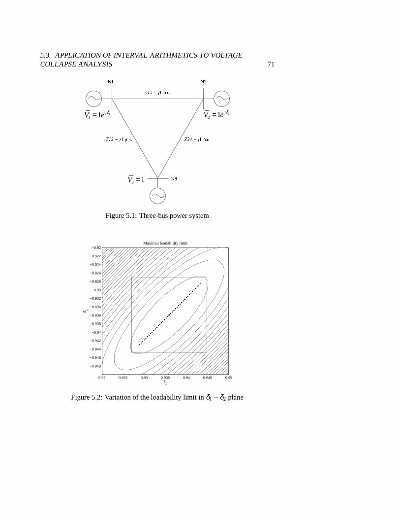
5.3. APPLICATION OF INTERVAL ARITHMETICS TO VOLTAGECOLLAPSE ANALYSIS 71
11 1 jV e δ= 2
2 1 jV e δ=
3 1V =
Figure 5.1: Three-bus power system
0.92 0.925 0.93 0.935 0.94 0.945 0.95
−0.948
−0.946
−0.944
−0.942
−0.94
−0.938
−0.936
−0.934
−0.932
−0.93
−0.928
−0.926
−0.924
−0.922
−0.92
δ1
δ 2
Maximal loadability limit
Figure 5.2: Variation of the loadability limit inδ1−δ2 plane

72CHAPTER 5. ASSESSMENT OF VOLTAGE STABILITY OF UNCERTAIN
POWER SYSTEMS
−1.2 −1.18 −1.16 −1.14 −1.12 −1.1 −1.08 −1.06 −1.04 −1.02 −1
−1.92
−1.9
−1.88
−1.86
−1.84
−1.82
−1.8
−1.78
δ1
δ 2
Saddle node bifurcation
Figure 5.3: Variation of the Saddle-node bifurcation point inδ1−δ2 plane
Due to the uncertainP1 andP2, the critical points of the system assume certainvalues which can be computed by a repetitive use of either the direct method i.e.,minimizing (5.5) [or (5.6)] for various combinations(p1, p2) : p1 ∈ [P1], p2 ∈ [P2]or by using the continuation method. However, both these methods can be quiteexpensive numerically. Alternatively, the objective function (5.7) [or (5.8)] can beminimized only once yielding the desired result directly. That is, upon minimizingthe interval-valued objective functions, we can directly find such an enclosure[u∗]that contains the set ofall values which the critical points of interest assume forthe parameters[P1] and[P2].
In the first experiment the following numerical values are chosen[P1] = [0.5±5·10−3] and[P2] = [−0.5±5·10−3] and a local minimum of (5.7) is sought. This op-timization problem was solved and the following numerical values were obtained:[λ1] = [3.4903,3.5504], [λ2] = [3.4903,3.5504]. Fig. 5.2 further illustrates the re-sults of the optimization. In the figure, the large box encloses the subset of theδ1− δ2 plane that is guaranteed to contain all critical points corresponding themaximal loadability of the system for allp1 ∈ [P1] andp2 ∈ [P2].
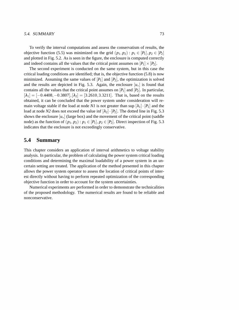
5.4. SUMMARY 73
To verify the interval computations and assess the conservatism of results, theobjective function (5.5) was minimized on the grid(p1, p2) : p1 ∈ [P1], p2 ∈ [P2]and plotted in Fig. 5.2. As is seen in the figure, the enclosure is computed correctlyand indeed contains all the values that the critical point assumes on[P1]× [P2].
The second experiment is conducted on the same system, but in this case thecritical loading conditions are identified; that is, the objective function (5.8)is nowminimized. Assuming the same values of[P1] and[P2], the optimization is solvedand the results are depicted in Fig. 5.3. Again, the enclosure[u∗] is found thatcontains all the values that the critical point assumes on[P1] and[P2]. In particular,[λ1] = [−0.4408,−0.3807], [λ2] = [3.2610,3.3211]. That is, based on the resultsobtained, it can be concluded that the power system under considerationwill re-main voltage stable if the load at nodeN1 is not greater than sup[λ1] · [P1] and theload at nodeN2does not exceed the value inf[λ2] · [P2]. The dotted line in Fig. 5.3shows the enclosure[u∗] (large box) and the movement of the critical point (saddlenode) as the function of(p1, p2) : p1 ∈ [P1], p2 ∈ [P2]. Direct inspection of Fig. 5.3indicates that the enclosure is not exceedingly conservative.
5.4 Summary
This chapter considers an application of interval arithmetics to voltage stabilityanalysis. In particular, the problem of calculating the power system criticalloadingconditions and determining the maximal loadability of a power system in an un-certain setting are treated. The application of the method presented in this chapterallows the power system operator to assess the location of critical points of inter-est directly without having to perform repeated optimization of the correspondingobjective function in order to account for the system uncertainties.
Numerical experiments are performed in order to demonstrate the technicalitiesof the proposed methodology. The numerical results are found to be reliable andnonconservative.


Part III
Power System Load Modelingand Identification
75

Chapter 6
Identification and Modeling ofAggregate Power System Loads
“A basic rule in estimation is not to estimatewhat you already know.”
— A quotation from [113]
This chapter addresses some theoretical and practical issues relevant to the prob-lem of modeling and identification of aggregate power system load. Two identifi-cation techniques are developed in the theoretical framework of stochasticsystemidentification. The identification techniques presented in this chapter belong tothe family of output error models; both techniques are based on well-establishedequations describing load recovery mechanisms having a commonly recognizedphysical appeal. Numerical experiments with artificially created data werefirstperformed on the proposed techniques and the estimates obtained provedto be as-ymptotically unbiased and achieved the corresponding Cramer-Rao lower bound.The proposed techniques were then tested using actual field measurements taken ata paper mill, and the corresponding results were used to validate a commonly usedaggregate load model.
The results reported in this chapter indicate that the existing load models sat-isfactorily describe the actual behavior of the physical load and can be reliablyestimated using the identification techniques presented herein.
6.1 IntroductionAccurate models of power system loads are essential for analysis and sim-ulation of the dynamic behavior of electric power systems [5]. Havingaccurate models of the loads that are able to reliably reflect underlying
phenomena of the physical loads is important for the purposes of designing auto-
77
78CHAPTER 6. IDENTIFICATION OF AGGREGATE POWER SYSTEM
LOADS
matic control systems and optimization of their configuration. More importantly,the dynamic properties of power system loads have a major impact on system sta-bility [5, 66, 122]. In particular, previous work on the subject of voltagestabilityreported in the literature indicates that the parameters of both static and dynamicloads have significant impact on voltage stability of the power systems [53, 122].On the other hand, the impact of power system load models on inter-area oscilla-tions is discussed in [5], demonstrating the influence that load parameters have onthe dominant system eigenvalues. This dependence reveals the link between theeffectiveness of power system damping controllers (e.g., power systemstabilizersor PSS) and the correctness of the eigenstructure of the system, which is dependenton the load model.
To be able to predict the behavior of a system, reliable models of system compo-nents are needed that faithfully reflect the dynamical behavior of the actual physicalcomponents of the system. Most of the power system components can be satisfac-torily modeled by considering the physical laws which govern the respective com-ponents. There are, however, some cases when power system modelingis quite acomplicated exercise. Modeling power system loads is one of them. It is knownthat at high voltage levels, the power system loads have to be aggregated inorderto obtain manageable models suitable for analysis and simulations [5]. Dependingon the load type (e.g. lighting, motor load, heating, etc.), the parameters of theaggregate load model may vary in a wide range. When the parameters of all loadcomponents are well known, the parameters of the aggregate load models can bereadily determined. If the parameters of separate loads are not known orthe loadstructure is known, but the proportion of various load components is not, derivingan aggregate load becomes more difficult.
It can be argued that in the absence of precise information about a power sys-tem load, one of the most reliable ways to obtain an accurate model of the load isto apply an identification technique. That is, if field measurements of load quan-tities (e.g., the voltage and current/power) adequately describing its behavior areavailable, then a dynamic and/or static equivalent of the load can be obtainedbyanalyzing functional relationships between these quantities.
The current chapter is concerned with theoretical and numerical aspects of iden-tification of an aggregate model of power system loads. Identification of both lin-ear and nonlinear models of a power system load is treated. Two identificationtechniques are presented that belong to the so-called family of output error models.First, the estimation of the load parameters using a linear model is presented, whichis followed by the presentation of a nonlinear identification technique. The statisti-cal properties of the proposed identification methods are studied both numerically

6.2. AGGREGATE MODELS OF POWER SYSTEM LOADS 79
and analytically. Thus, artificially created data are analyzed numerically andthevariance of the obtained estimates is compared with the corresponding Cramer-Rao lower bound. Then, in order to benchmark the identification techniquesandvalidate the analytical load models, field measurements taken at a paper mill wereused. The results obtained indicate that the load models describe the actual be-havior of the load with high accuracy. Moreover, it is shown that the load modelparameters can be accurately identified using the proposed techniques.
6.2 Aggregate Models of Power System Loads
In general, obtaining detailed models of power system loads is a more complicatedtask than modeling a particular power system component, such as, for instance, asynchronous machine. The problem is two-fold:
(a) Loads are time variant and stochastic;
(b) In most cases, at high voltage levels the loads must be aggregated.
The latter is due to the large number and types of loads connected at the transmis-sion system level, which makes the consideration of each separate load numericallyimpractical and provides no insight into the system analysis. The time varianceofloads can be accounted for by the explicit modeling their dynamic behavior bydifferential and/or difference equations.
Power system load aggregation can be performed in two ways:
(i) Analytically, by lumping similar loads and then using pre-determined valuesfor each parameter of the load (e.g. [3] and [4]) or
(ii) Selecting a load model and then performing parameter estimation using anappropriate identification technique.
Static load models
Due to the importance of adequate load modeling, a large number of various staticmodels of power system loads have been developed. Despite this diversity, in prin-ciple, they all serve one common goal: to reflect the voltage and possibly frequencydependence of the active and reactive components of the loads. For example, in [4]
80CHAPTER 6. IDENTIFICATION OF AGGREGATE POWER SYSTEM
LOADS
the following standard load models used for dynamic studies in established stabil-ity programs (e.g., EPRI’s LOADSYN and ETMSP packages) are suggested:
P = P0
[
Pa1
[VL
V0
]Kpv1
[1+Kp f1( f − f0)]+(1−Pa1)
[VL
V0
]Kpv2]
(6.1)
Q = P0
[
Qa1
[VL
V0
]Kqv1
[1+Kq f1( f − f0)]
+ [1+Kq f2( f − f0)]
[Q0
P0−Qa1
][VL
V0
]Kqv2]
(6.2)
whereVL and f are the load bus voltage and frequency, respectively. In equations(6.1)–(6.2),Kpv1 andKpv2 represent the voltage exponents for frequency dependentand frequency independent active power load;Kqv1 andKqv2 stand for the voltageexponents for the uncompensated and compensated reactive power load; Kp f1 andKq f1 are the frequency sensitivity coefficients for active and uncompensated reac-tive power load;Kq f2 is the frequency sensitivity coefficient for reactive compen-sation; andPa1 andQa1 represent the frequency dependent fraction of active loadand reactive load coefficient of uncompensated reactive load to activepower load,respectively.V0, P0, andQ0 denote the nominal values of the load voltage and ac-tive and reactive power of the load. It is important to note that in the models abovesome fraction of the load is explicitly modeled as a function of bus voltage, whilethe other fraction is as an explicit function of frequency.
The usefulness of a load model is directly related to the correctness of the para-meters of the model. The parameters can be obtained in two ways: pre-determinedvalues can be chosen based on the load type, or the parameters can be estimatedbased on field measurements. The latter is more expensive but it is preferable, sinceit can yield more accurate values of the load parameters.
The estimation of the parameters of a static load is relatively simple, as the loadmodel does not involve dynamical variables; in this case, the task of parameterestimation is practically reduced to curve fitting. References [35] and [132] reportsuccessful attempts to estimate static load parameters using a modified algorithmof Broyden, Fletcher, Goldfarb, and Shanno (BFGS) and a least squares technique,respectively. It should however be noted that the application of any gradient-basedoptimization routine can potentially lead to hitting a local optimum of the associ-ated objective function, and thus obtaining inaccurate parameter values.

6.2. AGGREGATE MODELS OF POWER SYSTEM LOADS 81
Dynamic load models
Nonlinear Dynamic Load Models
The impact that loads have on the dynamics of a power system has stimulatedsignificant research efforts directed towards proper modeling of certain character-istics of power system loads. In many cases the use of static load models may beinappropriate due to their failure to accurately reflect the influence of the load onsystem stability [4], [81]; hence, since some loads do exhibit dynamical behavior(e.g., motor loads), these are represented by means of dynamical models.
It has been shown in [5] and [53] that the following models of aggregate loadscan successfully capture the dominant nonlinear steady-state behavior of the loadas well as load recovery and overshoot:
x(t) =−x(t)Tp
+P0
[VL(t)
V0
]Nps
−P0
[VL(t)
V0
]Npt
Pd(t) =x(t)Tp
+P0
[VL(t)
V0
]Npt(6.3)
z(t) =−z(t)Tq
+Q0
[VL(t)
V0
]Nqs
−Q0
[VL(t)
V0
]Nqt
Qd(t) =z(t)Tq
+Q0
[VL(t)
V0
]Nqt(6.4)
In the equations abovePd(t) andQd(t) are the active and reactive power demandof the load,P0, Q0, andV0 stand for the nominal active, reactive power and voltage,respectively; the parametersTp andTq denote the time constant of the load internalstate variablesx(t) andz(t); and the exponentsNps, Nqs, Npt, andNqt are the steadystate and transient voltage indices. Observe that neglecting the frequency depen-dence in the static load model (6.1)–(6.2), the nonlinear load model (6.3)–(6.4) isequivalent to this model in steady state, i.e., for ˙x(t) = 0.
In the remainder of the chapter, the following notation will be usedy(t) := Pd(t)andθ = [Nps,Npt,T−1
p ]′= [θ1,θ2,θ3]′. In general, for a given load the exponentsθ1
andθ2 are not known exactly; however, similarly to the case of static load models,average values for many load types have been pre-determined. For example, [5]gives the following lower and upper bounds for these indices:
0 6 θ1 6 3, 0.5 6 θ2 6 2.5. (6.5)
82CHAPTER 6. IDENTIFICATION OF AGGREGATE POWER SYSTEM
LOADS
For simplicity, henceforth, the voltageV0, active and reactive powerP0,Q0 willbe assumed to be known values. Thus, the system voltage can be normalizedanddenoted by:V(t) := VL(t)/V0. In the subsequent sections of this chapter only themodel of active power (6.3) will be considered. The reactive power model givenby (6.4) can be treated in exactly the same manner.
It should be noted that the load models (6.3)–(6.4) are linear in the states; thenonlinearities enter the equations as inputs and outputs. Thus, strictly speaking,the model in the identification procedure discussed here should be referred to asa “Hammerstein-Wiener” model structure [42]. However, since these models areactually used in stability analysis of power systems, where load voltage magnitudesare treated as either algebraic or state variables, the model is typically referred toas a nonlinear model in this context. For this reason, and for the simplicity ofthe comparisons between the two different load models discussed here, thepresentmodel is referred to as a “nonlinear model” in the remainder of the chapter.
Linear Dynamic Load Models
When studying the behavior of a system in a small proximity of a given operatingpoint, the original nonlinear model can be approximated by a linear counterpart.That is, the nonlinear system can be linearized around the equilibrium point.Sincethe functionsVθ1(t) andVθ2(t) are smooth for a smoothV(t), the right-hand sidesof (6.3) can be expanded in a Taylor series, resulting in the linearized model of theload [53]:
∆x(t) = −θ3∆x(t)+P0(θ1−θ2)∆V(t)
= −A(θ)∆x(t)+B(θ)∆V(t)
∆y(t) = θ3∆x(t)+P0θ2∆V(t)
= A(θ)∆x(t)+D(θ)∆V(t). (6.6)
In principle, to obtain a rough estimate of the system behavior, pre-determinedvalues of the steady state and transient voltage indices can be used in simulations.However, as the transmission systems become more stressed, it becomes importantto have more accurate estimates of the indices, since they directly influence im-portant system characteristics such as damping; that is, incorporation ofinaccurateload characteristics in power system simulation models can lead to overestimationof system damping [81].

6.3. SYSTEM IDENTIFICATION 83
As in the case of static load models, the load characteristics can be identifiedbased on field measurements. The use of identification techniques can yield accu-rate estimates of load parameters, provided certain care has been exercised whenselecting input signals and setting up the measurement circuits. These and relatedquestions are treated in more detail in the next section.
6.3 System Identification
System identificationcan be defined as a collection of techniques which aim at ex-tracting a mathematical model of a given process by analyzing relations betweenthe input and output quantities of the process. Modern system identificationhas de-veloped into a mature engineering discipline which is intensively applied in manybranches of modern engineering. In this chapter, only identification techniquesthat are relevant to the problem at hand will be reviewed; for a detailed treatmentof system identification theory and practice the reader is referred to [79,80,89].
AutoRegressive Moving Average with eXternal input (ARMAX)method
In its simplest form, the procedure of process identification may be formulatedasfollows:
Given two vectors u,y find three sets of parameters ai ,bk,cl , i = 1,2, . . . ,n; k =1,2, . . . ,m; l = 1,2, . . . , p of a transfer function such that the model outputy bestfits the measured data y, being subjected to the same excitation signal u.The desired parameters can be found as shown below. Assume that the process
can be described by the model (6.7)
y(t)+a1y(t−1)+ · · ·+any(t−n)︸ ︷︷ ︸
A(q)y(t)
= b1u(t−1)+ · · ·+bmu(t−m)︸ ︷︷ ︸
B(q)u(t)
+e(t)+c1e(t−1)+ · · ·+cpe(t− p)︸ ︷︷ ︸
C(q)e(t)
(6.7)
or introducing the backward shift operatorq, equation (6.7) can be cast in the form
A(q)y(t) = B(q)u(t)+C(q)e(t), (6.8)
with the parameter vector
θ = [a1, . . . ,an,b1, . . . ,bm,c1, . . . ,cp]′ .

84CHAPTER 6. IDENTIFICATION OF AGGREGATE POWER SYSTEM
LOADS
Equation (6.8) can be reshaped by introducing ˆy(t|θ)–an estimate ofy(t):
C(q)y(t|θ) = B(q)u(t)+ [C(q)−A(q)]y(t) (6.9)
and further rearrangement of (6.9) yields:
y(t|θ) = B(q)u(t)+ [1−A(q)]y(t)+ [C(q)−1] [y(t)− y(t|θ)]︸ ︷︷ ︸
ε(t|θ)
(6.10)
= φ ′(t|θ)θ . (6.11)
Minimization of the prediction errorε(t|θ) will yield the desired result–the pa-rameterθ , i.e., the parametersai ,bk, andcl . Once an objective function has beenchosen, the minimization can be done in many ways. If the analyst has decidedthatthe objective function should be a quadratic function inθ , e.g., 1/2ε(t|θ)′ε(t|θ),then the optimization results in the closed form solution:
θ =
[
1N
N
∑t=1
φ(t)φ ′(t)
]−11N
N
∑t=1
φ(t)y(t) (6.12)
State space identification methods
Now suppose that a model of the process is given by the state space model:
x(t +1) = Ax(t)+Bu(t)+v(t)y(t) = Cx(t)+Du(t)+w(t),
(6.13)
wherev(t) andw(t) are the process and measurement noise [118]. The followingstatistical characteristics are given:
E [v(t1)v′(t2)] = R1(θ)δt1,t2
E [v(t1)w′(t2)] = R12(θ)δt1,t2 (6.14)
E [w(t1)w′(t2)] = R2(θ)δt1,t2,
whereR are covariance matrices. The aim of the identification is to obtain thematricesA,B, andC such that the response of model (6.13) best fits the measureddata.
The task is solved in several steps which involve solving a Riccati equationassociated with (6.13) and (6.14):
P = APA′+R1−[APC′+R12
][CPC′+R2
]−1[CPA′+R′12
]. (6.15)

6.3. SYSTEM IDENTIFICATION 85
Note that in (6.15) the argument of matricesR(θ) is suppressed for conciseness.Having foundP, one should compute the Kalman gain as
K =[APC′+R12
][CPC′+R2
]−1(6.16)
Next, one-step ahead predictions are calculated which can be further used for theunknown parameter determination:
x(t +1|t) = Ax(t|t−1)+Bu(t)+Ky(t)y(t) = Cx(t|t−1)+ y(t).
(6.17)
Subspace identification methods
Subspace identification methods are relatively new; however, they have alreadyproven to be a sound alternative to well-established identification algorithms.
The power of the subspace algorithms lies in the following facts:
• They provide a clear link to the “old” identification methods
• They are of intrinsic Multi-Input-Multi-Output (MIMO) nature
• They allow the engineer to robustly estimate a possible order of the plant(done through inspection of singular values of the identified model)
• They allow for a lucid geometrical interpretation which actively connectshuman’s intuition [93].
Recent research [40] indicates that the use of subspace identification techniques canbe utilized for the model-free Linear Quadratic Gaussian (LQG) controller design,which can be viewed as a very useful feature enabling the user to obtain an LQGcontroller without the need for identification of a process model.
Subspace identification methods exploit the so-called orthogonal projections of“the future outputs onto past and future inputs and the past outputs”. Mathemati-cally the task of system identification is solved in several steps [40].
Step 1Given two measurementsui andyk, i,k = 1,2, · · · ,N, form the input matrices forthe ‘past’ and ‘future’ signals:
U1 =
u0 u1 · · · uk−1
u1 u2 · · · uk...
......
...uBH−1 uBH · · · uBH+k−2
, (6.18)
86CHAPTER 6. IDENTIFICATION OF AGGREGATE POWER SYSTEM
LOADS
U2 =
uBH uBH+1 · · · uBH+k−1
uBH+1 uBH+2 · · · uBH+k...
......
...uBH+FH−1 uBH+FH · · · uBH+FH+k−2
, (6.19)
wherek is the number of columns1, BH andFH stand for the backward and for-ward prediction horizons (number of data samples used for backward/forward pre-diction), respectively. According to [93], the prediction horizons must be “largeenough”.U1 andU2 denote matrices containing the ‘past’ and ‘future’ signals. Ina similar manner matricesY1 andY2 for the outputyk are formed.
Step 2Define the new matrixW1 = [Y′1,U
′1]′ and then calculate the matricesLw andLu:
Y2/
[W1
U2
]
= Y2[W′1U
′2
][
W1W′1 W1U ′2U2W′1 U2U ′2
]†[W1
U2
]
(6.20)
= LwW1 +LuU2 (6.21)
In equation (6.20), the operator ‘†’ is understood as the Moore-Penrose pseudo-inverse. For any square nonsingular matrixR, its pseudo-inverseR† = R−1. If Ris a non-square matrix and the following holds:R†RR† = R†,RR†R= R,(R†R)′ =R†R,(RR†)′ = RR†, thenR† is the pseudo-inverse ofR.
Step 3The procedure terminates by computing the singular value decomposition (SVD)of Lw and estimating of the future output ˆx1 [45]:
Lw = [Ua Ub]
[Sa 00 Sb
][V ′aV ′b
]
, (6.22)
whereUa,Ub are the output singular vectors,Va,Vb are the input singular vectors,andSa,Sb are the singular values of the matrixLw.
x1 = S1/2a V ′aW1. (6.23)
Concluding remarks on system identification
The main reasons for using identification techniques in power systems are theuncertain nature of the power system and ageing of power system components.
1In [40], it is noted thatk has to approach infinity in order to attain unbiased estimates.

6.3. SYSTEM IDENTIFICATION 87
Of course, it is preferable to explore every possibility of developing models ofthe system based on physical insights in order “not to estimate what we alreadyknow” [113]. Often a combination of modeling based on physical insights andsystem identification yields best results.
Power System Load Identification
In the context of this chapter, the load voltage and load power comprise the pair ofinput and output signals. It can be noticed that both models (6.3) and (6.4)describethe dynamic behavior of a load as functions of the nodal voltage in a noise-freeenvironment i.e., the presence of noise is not reflected in the models. Hence, toaccount for the presence of noise in the measurements and since no informationis available regarding the noise model, an output error model is chosen, whichis known to be robust and have a plausible physical interpretation. To simplifynotation, two new functionsu1(θ) andu2(θ) are introduced:
u1(θ) := P0Vθ1(t)−P0V
θ2(t)
u2(θ) := P0Vθ2(t)
Now, the model (6.3) can be reformulated in a stochastic framework as:
x(t) =−θ3x(t)+u1(θ)
y(t) = θ3x(t)+u2(θ)+e(t)
= y(t)+e(t).
(6.24)
In the equation above, the terme(t) represents white Gaussian noise with knownstatistics. Similar arguments apply to the model of reactive power.
Model discretization
Since measurements used in system identification are collected at predefinedin-stants of time, the continuous-time load equations (6.24) should be converted todiscrete-time counterparts. In this work, the discrete-time description of the loadequations is based on the Zero-Order Hold method (ZOH) and is obtained asfol-lows [124]:
x(kℓ+ ℓ) = F(θ)x(kℓ)+H(θ)u1(kℓ) (6.25)
y(kℓ) = θ3x(kℓ)+u2(kℓ)+e(kℓ) (6.26)
88CHAPTER 6. IDENTIFICATION OF AGGREGATE POWER SYSTEM
LOADS
whereℓ := tk+1− tk,∀k ∈ I ⊆ N, stands for the sampling interval, and the vari-ablesF(θ) andH(θ) are:
F(θ) := exp(−θ3ℓ), (6.27)
H(θ)u1(kℓ) =∫ kℓ+ℓ
kℓexp(θ3(kℓ+ ℓ− τ))u1(τ)dτ
= (1−F(θ))θ−13 u1(kℓ). (6.28)
In equation (6.28), it is assumed that the input functionu1(τ) is constant and equalto u1(kℓ) for kℓ 6 τ 6 kℓ+ ℓ.
Several numerical experiments conducted in the framework of this thesis con-firmed that ZOH discretization yields the least error as compared with other meth-ods such as, for instance, the forward Euler and the trapezoidal methods. Thus,ZOH is used here to discretize the nonlinear equations (6.24).
Prediction Error for the Nonlinear Load Model
The discretized equations can be utilized as a basis for the prediction of futureoutputs of the dynamic system, i.e.,
qx(kℓ) − F(θ)x(kℓ) = H(θ)u1(kℓ)
x(kℓ) = (q−F(θ))−1H(θ)u1(kℓ)
y(kℓ|θ) = θ3(q−F(θ))−1H(θ)u1(kℓ)
+u2(kℓ)e(kℓ)
=1−F(θ)
q−F(θ)u1(kℓ)+u2(kℓ)+e(kℓ)
= y(kℓ|θ)+e(kℓ). (6.29)
In equation (6.29), the symbolq denotes the forward shift operator. It is interestingto observe that the predicted value of the system output ˆy(k|θ) at timek equals thesum of the pre-filtered input functionu1(k) and input functionu2(k). Finally, theprediction error is defined as the difference between the predicted and actual outputof the system
ε(k|θ) = y(k)− y(k|θ), ∀k∈I . (6.30)
6.3. SYSTEM IDENTIFICATION 89
Prediction Error for the Linear Load Model
Similarly to the nonlinear load model, let us assume that the dynamic response ofthe load can be satisfactorily described by a linear output error model, i.e.,
∆y(t) = A(θ)∆x(t)+D(θ)∆V(t)+e(t). (6.31)
Applying the ZOH method to linearized load model (6.6), one readily obtains thediscrete load model:
∆x(kℓ+ ℓ|θ) = F(θ)∆x(kℓ)+Γ(θ)∆V(kℓ)
∆y(kℓ|θ) = A(θ)∆x(kℓ)+D(θ)∆V(kℓ)+e(kℓ), (6.32)
where (6.32),Γ(θ) = H(θ)P0(θ1− θ2), whereF(θ) andH(θ) are defined as in(6.27) and (6.28), respectively.
Eliminating the state variable∆x(kℓ), the discretized output error model (6.32)can be rewritten in the form of a transfer function:
∆y(kℓ|θ) =θ3Γ(θ)
q−F(θ)∆V(kℓ)+e(kℓ)
= P01−F(θ)
q−F(θ)(θ1−θ2)∆V(kℓ)+e(kℓ)
= ∆y(kℓ|θ)+e(kℓ). (6.33)
The prediction error for the linearized model is formulated as the difference be-tween the measured output∆y(kℓ) and the predicted output∆y(kℓ):
ε(k|θ) = ∆y(kℓ)−∆y(kℓ|θ), ∀k∈I . (6.34)
Minimization of the Prediction Error
Ideally, in a noise-free environment the prediction error is zero at all times, if bothload model and the values of the parameter vectorθ are known exactly. In practice,however, this is not achievable due to the fact that these conditions are not satisfied;moreover, field measurements always contain noise. Therefore, in the best casescenario, one can hope for keeping the prediction error reasonably small, which

90CHAPTER 6. IDENTIFICATION OF AGGREGATE POWER SYSTEM
LOADS
can be accomplished by formulating an optimization problem in which certain ob-jective function—often a 2-norm of the prediction error vector—is minimized byvarying the parameter vectorθ over the feasible parameter space. We thus followthe system identification tradition and define the optimization problem as
θ ∗ = argminθ∈Ω
12N‖ε(θ)‖22 . (6.35)
In the expression above,N is the number of data samples,θ ∗ and Ω stand forthe optimal parameter vector and the feasible parameter space defined by (6.5),respectively.
The success of prediction error minimization depends on a number of factors,namely,
(i) The optimization technique applied
(ii) The availability of a reasonable initial vectorθ0, and
(iii) The properties of the objective function.
While the first two factors in most practical cases can be relatively easy overcome,non-convexity of the objective function can in general represent a significant chal-lenge for all gradient-based optimization techniques. In order to avoid the traps oflocal minima, a robust minimization technique capable of finding the global opti-mum has been applied in the work reported in this chapter. A brief descriptionofthis optimization method as well as the techniques used to determine the varianceof the estimates are given below.
Adaptive Simulated Annealing
Simulated annealing (SA) can be defined as a family of general-purpose con-strained optimization algorithms whose operational principles imitate the processof crystal formation in solids during gradual cooling [92], [119].
The key idea behind SA algorithms is the analogy with the thermodynamicalprocess of cooling of a substance and subsequent formation of regular crystals.It has been discovered that when slowly cooled, the molecules of the substancetend to assume spatial positions which minimize the total potential energy of thesubstance. Analogously, in SA optimization routines a certain objective functionrepresents the potential energy of the substance, the parameters to be optimizedcan be thought of as the molecules of the substance. The analogy is completed byintroducing an artificial parameter that represents the temperature of the substance.
6.3. SYSTEM IDENTIFICATION 91
The invention of SA is credited to Metropolis [83]; however, its widespreaduse was initiated by Kirkpatrick’s work [70]. Simulated annealing algorithms havealready been applied to a large number of optimization problems such as powersystem planning and dynamic security assessment, spectral analysis estimation,signal detection, image processing and many other.
The main strength of SA algorithms lies in the fact that they are capable offinding the global optimum of a given objective function. This is achieved byin-troducing the so-called acceptance probability which allows avoiding local optima.The simplest implementation of an SA algorithm involves the following steps.
• Selection of an initial guessθ0 of the parameter vectorθ .
• Formulation of the objective functionJ(θ) and temperature scheduleTk(∆Jk,k),wherek is the iteration number. Evaluation of the objective function atθ0.
• Setting the so-called generating probability function, i.e., the function thatwill govern the formation of random perturbations to the current parametervectorθ .
• Setting the acceptance probability which is described by the Boltzmann dis-tribution pk(∆Jk,Tk).
• Generation ofr perturbationsθ (r) in proximity toθ0 and computing the cor-responding∆J(r)
k = J(r)k −Jk. If θ (r) yields an increase of the objective func-
tion, it is accepted as the new parameter vector, i.e.,θ ← θ (r), otherwise it isaccepted with the probabilityp(r)
k = exp(∆J(r)k /Tk).
• Selection of a stopping criterion and checking if the stopping criterion issatisfied.
• The iteration number is increased and the temperature is reduced.
It is known that simulated annealing algorithms are statistically guaranteed to findglobal optima, provided the temperature schedule, generating probability function,and acceptance probability are properly chosen [111]. It should however be notedthat simulated annealing has some drawbacks, one of which is slow convergencerate.
Several modifications have been made to the basic SA algorithms in an attemptto improve its performance. One of the most successful SA variations was devel-oped by L. Ingber [59] and termedAdaptive Simulated Annealing(ASA). Due to a

92CHAPTER 6. IDENTIFICATION OF AGGREGATE POWER SYSTEM
LOADS
new temperature schedule withTk decreasing exponentially in time and utilizationof re-annealing ASA performs significantly better that the basic SA algorithmandalgorithms based on Cauchy annealing.
The reasonable performance of ASA combined with the ability to locate globaloptima make its use suitable for the optimization tasks studied in this chapter.
Cramer-Rao Lower Bound for the nonlinear load model
Determination of an optimalθ ∗ satisfying (6.35), constitutes the first step of theload identification procedure presented in this chapter. The second step involves thecomputation of the variance of the estimates to assess the “quality” of the proposedidentification procedure. The variance of the estimates depends on several factors,among which the most important for the application discussed here are the numberof data samples available, the variance of noisee(t), the model of the load, and theinput signal.
To assess the minimum variance of the unknown parameters, the so-calledCramer-Rao Lower Bound (CRLB) is often used. By definition, CRLB is an in-verse of the Fisher Information Matrix (FIM)
FIM = E
((∂ lnL(θ ,N)
∂θ
)′ ∂ lnL(θ ,N)
∂θ
)
, (6.36)
whereN is the number of data samples available andE (ξ ) is the expected valueof ξ . The maximum likelihood function lnL(θ ,N) is defined in terms of the corre-sponding probability density functionL(θ ,N) as follows:
L(θ ,N) =(2π)−N/2√
det(W)exp
[
−12
[y− y]′W−1 [y− y]
]
=(2π)−N/2√
det(W)exp
[
−12‖y− y‖2W−1
]
(6.37)
In equation (6.37),W is a symmetric matrix representing the covariance of whiteGaussian noisee(t). This matrix can be used as an instrument to accentuate reliableparts of the measured datay. Often it is assumed thatW = σ2IN, whereIN is theidentity matrix andσ2 is the variance ofe(t). Without significant loss of generality,in the remainder of this chapter it is assumed thatW ≡ IN, which renders the twonorms‖ · ‖2 and‖ · ‖W−1 equivalent.
The derivation of CRLB for the parameter vectorθ requires the computationof the gradient of the maximum likelihood function, which is equivalent to the
6.3. SYSTEM IDENTIFICATION 93
gradient of the objective function in (6.35). The gradient is computed as follows:(for notational simplicity the argumentθ is suppressed in the following)
12N
∂‖ε(θ)‖22∂θ
=1
2N∂ (ε ′ε)
∂θ
=1
2N
[∂ε ′
∂θε +(ε ′⊗ In
) ∂ε∂θ
]
=1N
∂ε ′
∂θε, (6.38)
where the Jacobian matrix∂ε ′/∂θ is defined by
∂ε ′
∂θ=
∂ε1
∂θ1
∂ε2
∂θ1· · ·
∂εn
∂θ1∂ε1
∂θ2
∂ε2
∂θ2· · ·
∂εn
∂θ2∂ε1
∂θ3
∂ε2
∂θ3· · ·
∂εn
∂θ3
(6.39)
and the partial derivatives are
∂εk
∂θ1=
F(θ)−1q−F(θ)
P0Vθ1(k) lnV(k)
∂εk
∂θ2=
1−qq−F(θ)
P0Vθ2(k) lnV(k)
∂εk
∂θ3= ℓF
1−q(q−F(θ))2u1(k).
(6.40)
It should also be noted that for the load model adopted in this chapter, i.e., thatgiven by (6.25)–(6.26), the CRLB explicitly depends on both the input signalV(k)and the sampling intervalℓ. Moreover, by direct inspection of equations (6.39)and (6.40), one can immediately conclude that forV(k)≡ 1∀k, the matrix∂ε ′/∂θlooses rank and as a resultFIM becomes singular indicating that the variance ofθ is infinite; that is, the parametersθ are not identifiable, when the voltage is atsteady state(V(t) = V0).
It should be noted that the Jacobian (6.39) can be utilized to enhance the iden-tification procedure by excluding the parametersθi that are weakly identifiable ornon-identifiable [27], [57]. That is, one can use the algorithm proposed in [27] todetermine which load parametersθi cannot be reliably identified from the availablefield measurements. This can be done in the following 5 steps.

94CHAPTER 6. IDENTIFICATION OF AGGREGATE POWER SYSTEM
LOADS
1. Decompose∂ε ′/∂θ := VΛV ′.
2. Inspect the eigenvalues of the Jacobian, i.e., the diagonal elements of the ma-trix Λ. Determine the numberρ which is equal to the number of eigenvaluesof the Jacobain which are greater than some threshold value. This numberindicates the number of identifiable parameters.
3. PartitionV := V1⊕V2, whereV1 ∈ RN×ρ consists of the firstρ columns of
matrixV.
4. FactorizeV ′1 to obtain the orthonormal basis of the range space ofV ′1, theupper triangular matrixR, and the permutation matrixP, i.e.,V ′1P := QR.
5. UseP to determine the parametersθi that should not be identified but ratherset to some (approximate) values which are know beforehand.
The study reported in [27] indicates that this algorithm allows a significant reduc-tion of the variance of the estimates of theρ parameters even when the exact valuesof the non-identifiable parameters are unknown. A more detailed descriptionof thealgorithm and its applications can be found in [27], [57]. Numerical experimentsconducted in the framework of this study show that for the typical values oftheload parameters the Jacobian matrix is always well-conditioned implying that all3 parameters are identifiable; thus this algorithm is not applied in the case studydiscussed here.
6.4 Application Examples
Artificial data
In order to investigate the statistical properties of the identification procedure pre-sented in this chapter, a series of experiments is conducted using artificially createddata. Thus, in this section, the following issues are addressed:
• It is shown numerically that the estimates are asymptotically unbiased, whichwould not have been the case if an unreasonable predictor was chosen.
• A rough estimate of the magnitude of bias that can be expected for the lin-earized model (6.33) is obtained, which is a basic issue in system identifica-tion that has not yet been addressed in the current literature in load modeling.
6.4. APPLICATION EXAMPLES 95
• The adequacy of the optimization routine, i.e. an adaptive simulated anneal-ing algorithm, used in the chapter is demonstrated, as the method is able tolocate the global minimum of the objective function in all experiments.
The data vectory(tk) is generated with the help of a model with known parametersθ ; the outputy(tk) is then corrupted by Gaussian noise having known statistics,i.e.,e(t)∼N (0,σ2I) and the identification procedure is applied. The estimates ofthe parameter vectorθ are analyzed in this case to assess the performance of theproposed technique.
The main goal of the numerical experiments in this section is to investigate theasymptotic behavior of the variance of the estimatesθ(N). In other words, thefollowing relation has to be verified numerically:
limN→∞
varθ(N) = 0 (6.41)
for both linear and nonlinear load models. In expression (6.41) the operator varis defined as varξ = E (ξ 2), whereξ is a stochastic variable. To study the vari-ance of estimates, the value ofN is steadily increased and for each value ofN, aseries of Monte-Carlo simulations is performed. The variance is then computedand plotted versus the number of samplesN. In this case study, the data are gen-erated using the discrete-time model (6.25)–(6.26). The Monte-Carlo simulationsinvolve 30 runs for eachN, and the noise has the statisticsN (0,0.0015) withθ = [1.2 2.7 0.3448]′. The adaptive simulated annealing optimization routine isinitialized with θ0 = [0.5 2.0 1.7]′; and the feasible regionΩ is given by (6.5), andthe additional inequality 06 θ3 6 10.
The results of the Monte-Carlo simulations are shown in Figures 6.1 and 6.2.Several important observations can be made regarding the performanceof the
nonlinear model-based identification technique:
• All three parametersθi are accurately estimated by applying the identifica-tion algorithm to noisy data.
• The variance of the estimates decreases as the number of samples increases.This result indicates that the estimateθ is asymptotically unbiased, i.e.,equation (6.41) holds. This could be expected since minimization of (6.35)is equivalent to maximization of the maximum likelihood function, whichyields asymptotically unbiased estimates [79].
• For allN the variance of the estimates is insignificantly greater than the cor-responding CRLB, which implies that the proposed estimator is statisticallyefficient.

96CHAPTER 6. IDENTIFICATION OF AGGREGATE POWER SYSTEM
LOADS
100 200 300 400 500 600 700 800 900 100010
−6
10−5
10−4
10−3
10−2
10−1
Variance of θ vs number of data samples
log 1
0(va
r(θ))
Number of data samples, N
var(θ3)
var(θ1)
var(θ2)
CRLB(θ3)
CRLB(θ1)
CRLB(θ2)
Figure 6.1: Variance of the estimated parameter vectorθ versus number of sam-ples and the corresponding Cramer-Rao Lower Bounds for the artificial data set.Nonlinear load model
100 200 300 400 500 600 700 800 900 100010
−6
10−5
10−4
10−3
10−2
10−1
log 1
0(va
r(θL))
, log
10(v
ar(θ
NL))
Number of samples, N
var(θ3NL)
var(θ1NL)
var(θ2NL)
var(θ3L)
var(θ1L)
var(θ2L)
Figure 6.2: Variance of the estimates of the linear and nonlinear model parameters
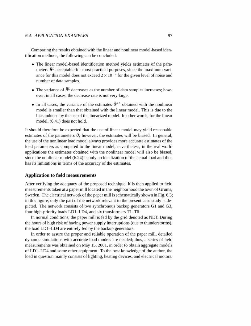
6.4. APPLICATION EXAMPLES 97
Comparing the results obtained with the linear and nonlinear model-based iden-tification methods, the following can be concluded:
• The linear model-based identification method yields estimates of the para-metersθ L acceptable for most practical purposes, since the maximum vari-ance for this model does not exceed 2×10⁻² for the given level of noise andnumber of data samples.
• The variance ofθ L decreases as the number of data samples increases; how-ever, in all cases, the decrease rate is not very large.
• In all cases, the variance of the estimatesθ NL obtained with the nonlinearmodel is smaller than that obtained with the linear model. This is due to thebias induced by the use of the linearized model. In other words, for the linearmodel, (6.41) does not hold.
It should therefore be expected that the use of linear model may yield reasonableestimates of the parametersθ ; however, the estimates will be biased. In general,the use of the nonlinear load model always provides more accurate estimatesof theload parameters as compared to the linear model; nevertheless, in the real worldapplications the estimates obtained with the nonlinear model will also be biased,since the nonlinear model (6.24) is only an idealization of the actual load and thushas its limitations in terms of the accuracy of the estimates.
Application to field measurements
After verifying the adequacy of the proposed technique, it is then appliedto fieldmeasurements taken at a paper mill located in the neighborhood the town of Grums,Sweden. The electrical network of the paper mill is schematically shown in Fig.6.3;in this figure, only the part of the network relevant to the present case study is de-picted. The network consists of two synchronous backup generators G1 and G3,four high-priority loads LD1–LD4, and six transformers T1–T6.
In normal conditions, the paper mill is fed by the grid denoted as NET. Duringthe hours of high risk of having power supply interruptions (due to thunderstorms),the load LD1–LD4 are entirely fed by the backup generators.
In order to assure the proper and reliable operation of the paper mill, detaileddynamic simulations with accurate load models are needed; thus, a series of fieldmeasurements was obtained on May 15, 2001, in order to obtain aggregate modelsof LD1–LD4 and some other equipment. To the best knowledge of the author, theload in question mainly consists of lighting, heating devices, and electrical motors.
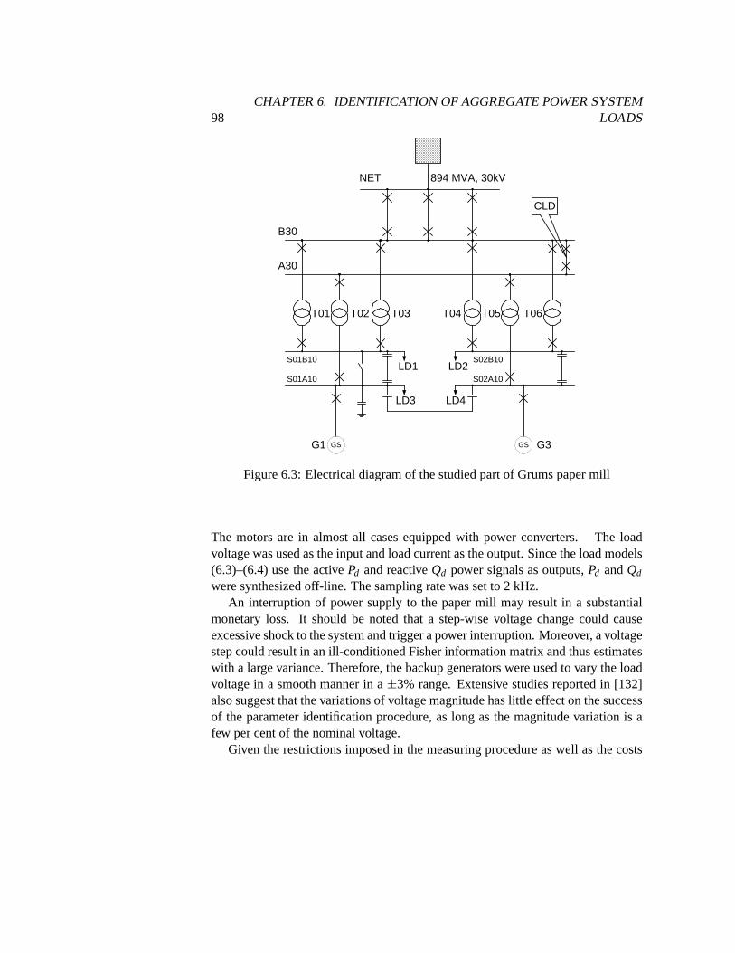
98CHAPTER 6. IDENTIFICATION OF AGGREGATE POWER SYSTEM
LOADS
T01 T02 T03 T04 T05 T06
NET
G1 G3
LD1 LD2
894 MVA, 30kV
LD3 LD4
B30
A30
S01B10 S02B10
S01A10 S02A10
CLD
GS GS
Figure 6.3: Electrical diagram of the studied part of Grums paper mill
The motors are in almost all cases equipped with power converters. The loadvoltage was used as the input and load current as the output. Since the loadmodels(6.3)–(6.4) use the activePd and reactiveQd power signals as outputs,Pd andQd
were synthesized off-line. The sampling rate was set to 2 kHz.An interruption of power supply to the paper mill may result in a substantial
monetary loss. It should be noted that a step-wise voltage change could causeexcessive shock to the system and trigger a power interruption. Moreover, a voltagestep could result in an ill-conditioned Fisher information matrix and thus estimateswith a large variance. Therefore, the backup generators were used tovary the loadvoltage in a smooth manner in a±3% range. Extensive studies reported in [132]also suggest that the variations of voltage magnitude has little effect on the successof the parameter identification procedure, as long as the magnitude variation isafew per cent of the nominal voltage.
Given the restrictions imposed in the measuring procedure as well as the costs

6.4. APPLICATION EXAMPLES 99
0 10 20 30 40 50 60 70 80 900.9
0.95
1
1.05
1.1
Time [s]
Nor
mal
ized
act
ive
pow
er: m
easu
red
and
sim
ulat
ed [p
.u.] Load identification. Linear model
θ1 = 2.3326
θ2 = 1.8778
θ3 = 1/9.9788
Load voltage
Measured power
Simulated power
Figure 6.4: Application of the proposed identification scheme to field measure-ments. Estimation of the parameters of active power load. Linearized model
associated with obtaining these measurements, it was only feasible to gather oneset of data at the given operating conditions. Hence, the cross-validation procedureapplied here is based on a comparison between the linear (6.6) and nonlinear (6.24)load models identified using the proposed procedure and based on the sameset offield measurements. Figures 6.4 and 6.5 depict the field measurements, i.e., theload voltage and active power, as well as the simulated outputsPd(t) of the linearand nonlinear models. Visual comparison of the measured and simulated powerindicate that both models capture the relevant dynamics of the load; however, thenonlinear model yields better results, showing a very close match with the fieldmeasurement, as these two curves are practically indistinguishable.
Table 6.1 presents the numerical values of the parameters obtained with bothlinear and nonlinear system identification techniques. In the table, the erroris de-fined as(θ NL
i − θ Li )/θ NL
i ·100%, whereθ Li and θ NL
i , i = 1,2,3 are the estimatesof the linearized and nonlinear model parameters, assuming the nonlinear model isthe reference for these calculations, given the close match between this model andthe actual measurements. The table reveals that the parameters identified with thelinear model do not deviate significantly from those obtained with the nonlinear

100CHAPTER 6. IDENTIFICATION OF AGGREGATE POWER SYSTEM
LOADS
0 10 20 30 40 50 60 70 80 900.9
0.92
0.94
0.96
0.98
1
1.02
1.04
1.06
1.08
1.1
θ1 = 2.3131
θ2 = 1.9445
θ3 = 0.1161
Time [s]
Nor
mal
ized
act
ive
pow
er: m
easu
red
and
sim
ulat
ed [p
.u.] Load identification. Nonlinear model
Load voltage
Measured power
Simulated power
Figure 6.5: Application of the proposed identification scheme to field measure-ments. Estimation of the parameters of active power load. Nonlinear Identification
Table 6.1: Comparison of the load parameters identified using linear and nonlinearmodels
Linear model Nonlinear model Error [%]
Nps [p.u.] 2.3326 2.3131 −0.8430Npt [p.u.] 1.8778 1.9445 3.4302T−1
p [s] 0.1002 0.1161 13.6951
6.5. SUMMARY 101
load identification technique. This is mainly due to the fact that the voltage devia-tion was not large and hence nonlinear effects were not very significant. However,observe that the maximum error introduced by the use of linearized model is stillgreater than 13%; hence, we may conclude from these results that the nonlinearmodel is a more accurate representation of the given aggregate load.
Notice that at different operating conditions, one would expect to obtain differ-ent values for the load parameters. However, based on the results depicted here andthe fact that the load composition is not expected to change significantly for typicaloperating conditions, it is reasonable to expect similar trends in terms of the accu-racy of the linear and nonlinear load models for representing the given aggregateload.
It is interesting to compare the values of load parameters obtained in this studywith those reported in the literature. For instance, [132] cites the following valuefor Nps = 0.72 for an industrial load. This value differs significantly from the oneshown in Table 6.1, which can be mainly explained by a different composition ofthe load. The steady state and transient voltage indices determined in [66] matchthose of the present case study somewhat more closely; however, the time constantsTp differ significantly, which can be explained by the absence of devices havingslow dynamics, e.g., OLTC in the present study.
6.5 Summary
Two power system load identification techniques are proposed in this chapter. Wellestablished equations describing the nonlinear recovery mechanisms of load formthe basis of both techniques, which are formulated in the framework of stochas-tic system identification theory. Specifically, a linear and nonlinear output errorestimators are introduced and analyzed, and generic equations applicableto iden-tification of aggregate models of power system loads are developed and studied indetail.
The asymptotic behavior of the estimates is studied by means of numerical ex-periments with artificially created data, demonstrating that the estimates are as-ymptotically unbiased for the nonlinear load model and their variance attains theCramer-Rao lower bound. To avoid numerical problems associated with possiblemultiple minima of the objective function, a global minimization technique wasutilized. The enhanced numerical features of the minimization routine enable fastconvergence to the global minimum of the objective function with a probabilityof 1.

102CHAPTER 6. IDENTIFICATION OF AGGREGATE POWER SYSTEM
LOADS
The theoretical foundations presented in this chapter were applied to field mea-surements taken at a paper mill located in the neighborhood of the town of Grums,Sweden. Both linear and nonlinear models were utilized in order to estimate theload parameters. The results show that, in principle, the linear model yields validestimates that differ from the estimates obtained using the nonlinear model. When-ever the accuracy requirements on the numerical values of the load parameters arenot stringent, linear identification can be applied for the estimation of the parame-ters. Alternatively, the nonlinear load modeling and identification technique pre-sented in this thesis can be used to better model the load and obtain more accurateestimates of the load parameters.

Part IV
Qualitative Analysis ofOperation, Control, and Stability
of Distributed Generation
103


Chapter 7
Design of Robust Control forEnhancing the Performance ofSOFC Power Plant
“He was under the impression that a system description(like the transfer function) is exactly the same
as a system in a concrete physical sense.”— R. Kalman [65]
On the flaws in the Wiener formulation.
This chapter presents a discussion on the load following capabilities of a powerplant that consists of solid oxide fuel cells (SOFC) and microturbines. Such apower plant, in theory, is capable of operating at unprecedented efficiencies whichcan be above 80%. However, as the analysis in this chapter shows, the load fol-lowing capabilities of this power plant can be unsatisfactory, due to certain con-trol limitations. To enhance the load following capabilities of the power plant,attenuate possible disturbances from the distribution grid, and avoid interactionbetween the control functionalities of the fuel cells and the microturbines, twoH∞ controllers are designed. The main emphasis in this chapter is placed uponthe behavioral features of the fuel cell plant itself rather than on the studying theintegrated system “fuel cell–distribution grid”. The exposition of the theoreticalmaterial in this chapter is rather axiomatic; however, this approach will certainlysuffice for the practical purposes of this work. We commence by giving abriefoverview ofH∞ control theory.
7.1 Robust ControlModeling of electric power systems is not a trivial task even if the engi-neer has succeeded in collecting all the necessary information about thepower system. Aging of power equipment and uncertain load1 complicate
1More specifically, both the level and composition of the load at a given instant of time areuncertain. In system planning studies, power system loads can be forecasted; however, neither type
105
106CHAPTER 7. DESIGN OF ROBUST CONTROL FOR SOFC POWER PLANT
modeling, analysis, and control of electric power systems.This feature of power systems suggests the choice of control strategy—robust
control—if precise and “guaranteed” control of some quantities, e.g., active poweroutput is required. It is quite likely that the potential of robust and optimal controltechniques will have the commanding influence on power engineering; however,this time is yet to come. For this and other reasons, the foundations ofH∞ controltheory are presented in detail in this chapter. It is hoped that this will help indisseminating these techniques among practicing electrical engineers.
The origins ofH∞ optimal control theory were established in the early 1980’sby G. Zames, see e.g., [133]. Since then it has been intensively studied bythe con-trol community. A brief introduction to this fascinating theory is given below. Thissections establishes the relationship between the robustness issue andH∞ -normminimization. Most of the section makes an extensive use of frequency domaindueto nice geometrical interpretations of the main concepts and follows chiefly [76];however, time-domain solutions to the standardH∞ problem are also presented. Itshould be noted that the presentation is fairly general, and the theory is applicableto a large class of linear time-invariant systems, whose transfer functions or statespace realizations are represented by either the capitalP or G, respectively. Thereis however a simple relationship between these two representations. For details onthe SOFC plant studied, the reader should refer to Section 3.2 and Appendix C.
The standardH∞ control problem can now be formulated. However, prior to theintroduction of theH∞ theory, it is instructive to introduce the main configurationof the controlled plant and controller itself. Fig. 7.1 shows the standard blockdiagram of the dynamic system which is controlled by an external controllerK. Itshould be stressed that the so-called weighting functions which are the main toolsfor fulfilling the control specifications are already absorbed into the plantG. At thepresent time, this will not be discussed, as the structure of the plant is different inthe setting for the frequency and time domains.
The main purpose of the linear robust controllers in this chapter is to providetight active power output control of the tandem SOFC–microturbines. Further-more, the models of the SOFC is assumed be deterministic; however, the terminalvoltage variations are treated as unstructured model uncertainty. The voltage vari-ations are assumed to be caused either by the operation of the microturbines or bythe disturbances on the distribution grid. Thus, in this study, the presence of themicroturbines is accounted for only indirectly.
Now the problem ofH∞ -controller synthesis can be stated
nor dynamical characteristics of the load are specified.
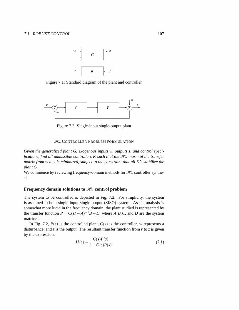
7.1. ROBUST CONTROL 107
G
K
-
- -w z
yu
Figure 7.1: Standard diagram of the plant and controller
PC ΣΣ - - --?
6–
rw
-z
Figure 7.2: Single-input single-output plant
H∞ CONTROLLER PROBLEM FORMULATION
Given the generalized plant G, exogenous inputs w, outputs z, and control speci-fications, find all admissible controllers K such that theH∞ -norm of the transfermatrix from w to z is minimized, subject to the constraint that all K’s stabilize theplant G.We commence by reviewing frequency-domain methods forH∞ controller synthe-sis.
Frequency domain solutions toH∞ control problem
The system to be controlled is depicted in Fig. 7.2. For simplicity, the systemis assumed to be a single-input single-output (SISO) system. As the analysisissomewhat more lucid in the frequency domain, the plant studied is represented bythe transfer functionP = C(sI−A)−1B+ D, whereA,B,C, andD are the systemmatrices.
In Fig. 7.2,P(s) is the controlled plant,C(s) is the controller,w represents adisturbance, andz is the output. The resultant transfer function fromr to z is givenby the expression:
H(s) =C(s)P(s)
1+C(s)P(s)(7.1)

108CHAPTER 7. DESIGN OF ROBUST CONTROL FOR SOFC POWER PLANT
The ratio(1+C(s)P(s))−1 is called thesensitivity functionof the feedback sys-tem, which characterizes the sensitivity of the compensated plant to various distur-bances.
Usually the sensitivity function is denoted by capitalS. In the ideal case, thesensitivity functionS should be zero. In practice it is, however, unrealistic to re-quire zero sensitivity. Instead, an upper bound on the peak value of thesensitivityfunction is specified for a certain range of frequencies. That is, one sets an upperlimit on ‖S‖∞:
‖S‖∞ = supω∈R
|S( jω)| . (7.2)
As is seen in (7.2), the sensitivity function is a function of frequency, assumingdifferent values for different frequencies. As this dependence is undesirable (dueto the possible magnification of noise and the influence of neglected dynamics), aweighting functionW( jω) is introduced in order to reduce the dependence.
‖WS‖∞ = supω∈R
|W( jω) ·S( jω)| . (7.3)
The loop gainL = PC is another quantity which plays an important role inH∞ op-timization and is closely connected to robustness of the system, see Fig. 7.2.
Due to the plant uncertainties (in power systems this can be the level of loadingof the system), the actual plant parameters differ from the nominal ones. To distin-guish between them, the loop gain of the actual plant is denoted byL and that ofthe nominal plant asL0. Both these plants are stable if the corresponding Nyquistplots do not encircle the point(−1, j · 0). Following in steps of [76], it may benoted that plant is stable if the following inequality holds:
|L( jω)−L0( jω)|< |L0( jω)+1| , ∀ω ∈ R. (7.4)
Graphical interpretation of the inequality is given by Fig. 7.3. Inequality (7.4) canbe rearranged as follows:
|L( jω)−L0( jω)|
|L0( jω)|·|L0( jω)|
|L0( jω)+1|< 1, ∀ω ∈ R (7.5)
The complementary sensitivity functionT0 of the closed loop plant is defined as:
T0 = 1−S0 = 1−1
1+L0=
L0
1+L0(7.6)

7.1. ROBUST CONTROL 109
0
ℑℜ
L
L0
(−1,0)
L( jω)
L0( jω)
6
-
o
Figure 7.3: Nyquist plot of the SISO system
In equation (7.6),S0 stands for the sensitivity function of the nominal plant. Equa-tions (7.5)–(7.6) can be combined to produce:
|L( jω)−L0( jω)|
|L0( jω)|· |T0( jω)|< 1, ∀ω ∈ R. (7.7)
The multiplier |L( jω)−L0( jω)|/|L0( jω)| is called therelative sizeof the per-
turbation of the gain loopL from its nominal valueL0. If the relative size of theperturbation is bounded, we can write:
|L( jω)−L0( jω)|
|L0( jω)|6 |W( jω)| , ∀ω ∈ R, (7.8)
whereW( jω) is the aforementioned (given) weighting function. The followingexpression can be obtained after simple manipulations:
|L( jω)−L0( jω)|
|L0( jω)|
1|W( jω)|
|T0( jω)W( jω)| < |W( jω) ·T0( jω)| , (7.9)
|W( jω) ·T0( jω)| < 1, ∀ω ∈ R. (7.10)
The last result can be interpreted as follows: for any disturbance that isboundedbyW( jω) (inequality (7.10) holds) the closed-loop plant remains stable (inequality
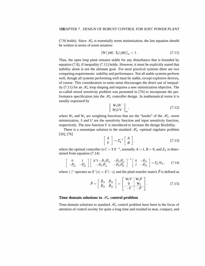
110CHAPTER 7. DESIGN OF ROBUST CONTROL FOR SOFC POWER PLANT
(7.9) holds). SinceH∞ is essentially norm minimization, the last equation shouldbe written in terms of norm notation:
‖W( jω) ·T0( jω)‖∞ < 1. (7.11)
Thus, the open loop plant remains stable for any disturbance that is bounded byequation (7.8), if inequality (7.11) holds. However, it must be explicitly statedthatstability alone is not the ultimate goal. For most practical systems there are twocompeting requirements: stability and performance. Not all stable systems performwell, though all systems performing well must be stable, except explosive devices,of course. This consideration in some sense discourages the direct useof inequal-ity (7.11) for anH∞ loop shaping and requires a new minimization objective. Theso-calledmixed sensitivity problemwas presented in [76] to incorporate the per-formance specification into theH∞ controller design. In mathematical terms it isusually expressed by
∥∥∥∥
W1SVW2UV
∥∥∥∥
∞, (7.12)
whereW1 andW2 are weighting functions that are the “knobs” of theH∞ -normminimization,S andU are the sensitivity function and input sensitivity function,respectively. The new functionV is introduced to increase the design flexibility.
There is a nonunique solution to the standardH∞ -optimal regulator problem[50], [76] [
XY
]
= Z−1λ
[AB
]
, (7.13)
where the optimal controller isC = YX−1, normallyA = I , B = 0, andZλ is deter-mined from equation (7.14)
[0 I−P∗12 −P∗22
][λ 2I − P11P∗11 −P11P∗21−P21P∗11 −P21P∗21
]−1[0 −P12
I −P22
]
= Z∗λ JZλ , (7.14)
where(·)∗ operates asX∗(s) = X′(−s) and the plant transfer matrixP is defined as
P =
[P11 P12
P21 P22
]
=
W1V W1P0 W2
−V −P
. (7.15)
Time domain solutions toH∞ control problem
Time-domain solutions to standardH∞ control problem have been in the focus ofattention of control society for quite a long time and resulted in neat, compact, and

7.1. ROBUST CONTROL 111
relatively “simple” expressions. Below we replicate the ones that will shortlybeused in the present thesis.
Some mathematical preliminaries which will facilitate the further treatmentopen this subsection.
Lemma 1 Let matrix H be defined as
H ,
[A RQ −A′
]
,
and suppose H∈ dom(Ric) and X= Ric(H). A,Q and R∈ Rn×n with Q and R
symmetric. Then:
1 X is symmetric.
2 λi(A+RX) < 0,∀ i.
3 X satisfies the algebraic Riccati equation A′X +XA+XRX−Q = 0.
A proof of the lemma and details on the notation used can be found in [36] and[134]. For now, the most important detail is thatX satisfies the associated Riccatiequation. This fact will be used when tackling with suboptimalH∞ controllers.
Unlike the situation with LQR, in the present case close-form solutions to theoptimalH∞ control problem cannot be obtained as the optimal control requires aniterative search over the set of all admissible controllers.
Let the transfer matrix of the plantG be partitioned as
G =
A B1 B2
C1 0 D12
C2 D21 0
(7.16)
and the following assumptions hold
a (A,B1) and (A,B2) are stabilizable.
b (C12,A) and (C21,A) are detectable2.
c D′12 = [0, I ].
d[
B1
D21
]
D′21 =
[0I
]
.
2The pair(C,A) is said to be detectable if for someL the matrixA+LC is a Hurwitz matrix.
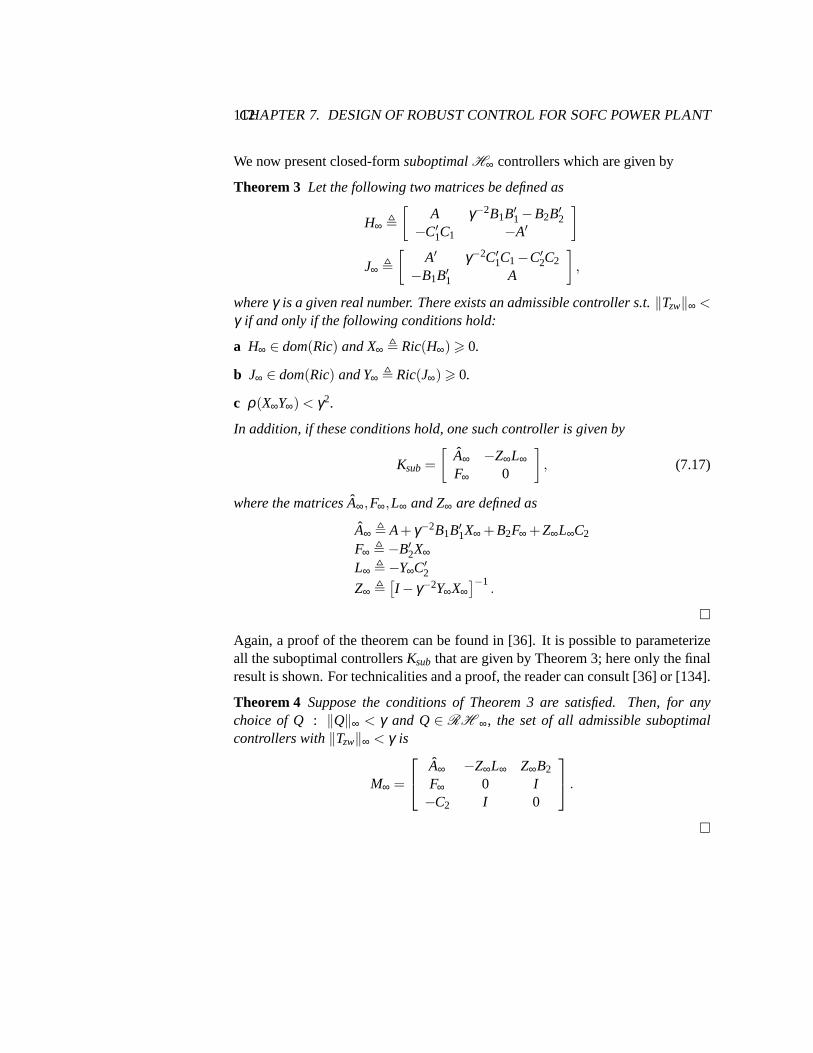
112CHAPTER 7. DESIGN OF ROBUST CONTROL FOR SOFC POWER PLANT
We now present closed-formsuboptimalH∞ controllers which are given by
Theorem 3 Let the following two matrices be defined as
H∞ ,
[A γ−2B1B′1−B2B′2
−C′1C1 −A′
]
J∞ ,
[A′ γ−2C′1C1−C′2C2
−B1B′1 A
]
,
whereγ is a given real number. There exists an admissible controller s.t.‖Tzw‖∞ <γ if and only if the following conditions hold:
a H∞ ∈ dom(Ric) and X∞ , Ric(H∞) > 0.
b J∞ ∈ dom(Ric) and Y∞ , Ric(J∞) > 0.
c ρ(X∞Y∞) < γ2.
In addition, if these conditions hold, one such controller is given by
Ksub=
[A∞ −Z∞L∞F∞ 0
]
, (7.17)
where the matricesA∞,F∞,L∞ and Z∞ are defined as
A∞ , A+ γ−2B1B′1X∞ +B2F∞ +Z∞L∞C2
F∞ ,−B′2X∞L∞ ,−Y∞C′2Z∞ ,
[I − γ−2Y∞X∞
]−1.
Again, a proof of the theorem can be found in [36]. It is possible to parameterizeall the suboptimal controllersKsub that are given by Theorem 3; here only the finalresult is shown. For technicalities and a proof, the reader can consult [36] or [134].
Theorem 4 Suppose the conditions of Theorem 3 are satisfied. Then, for anychoice of Q : ‖Q‖∞ < γ and Q∈ RH ∞, the set of all admissible suboptimalcontrollers with‖Tzw‖∞ < γ is
M∞ =
A∞ −Z∞L∞ Z∞B2
F∞ 0 I−C2 I 0
.

7.1. ROBUST CONTROL 113
M∞
Q
-- -y u
Figure 7.4: Parametrization of all suboptimalH∞ controllers
Figure 7.4 shows a schematic block diagram of the parameterized sub-optimalH∞ controllers.
To exemplify the theory presented earlier in this chapter, let us design anH∞ -controller for a single machine infinite bus (SMIB) system.
Example: Consider the SMIB system, which represents a simplified linearizedmodel of single generator connected to an infinite bus. The classical modelofthe generator is used in this example; that is, the generator is modeled by equations(3.3)–(3.4). The quantitiesE′q andE′d in equations (3.4) are assumed to be constant.The parameters of the system are chosen such that the generator exhibitsquite anoscillatory behavior. In this example we seek anH∞ controller that is capable ofstabilizing the SMIB system by regulating the mechanical power of the generator.
[δω
]
=
[0 100π
−0.05 −0.01
][δω
]
+
[0
0.1
]
u(t), (7.18)
y = C [δ ,ω ]′+Du, C = [1,0], D = 0.
The following frequency-domain control specifications are set3:
Closed-loop bandwidth: ωB = 12 rad/sec.
Peak of sensitivity function: Smax= 1.1.
Steady state: Approximate integral action at low frequencies.
Obj. function: For this example, selectingε = 10−6, the objective functions ischosen as
J(S,K) = argminK
∥∥∥∥
wPSKS
∥∥∥∥
∞, wP =
0.67s+10s+ ε
.
3These control specifications are set arbitrarily for demonstration purposes only; however, thesevalues are quite realistic.

114CHAPTER 7. DESIGN OF ROBUST CONTROL FOR SOFC POWER PLANT
TheH∞ -norm minimization is performed with the help of theµ-toolbox in MAT-LAB [20], which yields the value ofγ = 1.08. The resultant suboptimal controllerK(s) has following structure
K(s) =4617s2 +46.17s+7.254e4
s3 +4451s2 +3.64e4s+0.01348.
The SMIB system controlled byK has the following eigenvalues:λ1 = −4443
andλ2,3 =−1.8044± j4.3542. The input to theH∞ optimal controller is the angledeviation of the generator’s shaft and the output is the control signalu(t).
Note: It is worth mentioning that selection of weighting functions for the designof H∞ controller synthesis plays an essential role. As yet, selection of weightsin robust and optimal control is more art than science, since from case to case,different ad hoc approaches have to be tried in order to obtain “the bestdesign.”This example concludes the introduction to basics of theH∞ controller synthesis.
7.2 Application of Robust Control to the SOFC Plant
Motivation
Recent advances in the fuel cell technology significantly improved the technicaland economical characteristics of modern fuel cells making them more suitableand beneficial for the decentralized use of energy generation [55]. Environmentalfriendliness, practically noise free operation, and very high efficiencycombinedwith the forecasted shift to gaseous fuels make fuel cells a very sound competitoron the future electricity markets [22], [12]. In addition, it should be noted thatfuel cell-based generators possess other important properties such as compact size,modularity, and controllability.
It is shown in [56] and [135] that load following and regulation comprise asubstantial part of total interconnected operation services, which is likelyto stim-ulate the owners of DG’s to participate in the provision of this particular ancillaryservice. There are, however, some technical challenges associated with the fuelcell technology which can represent certain difficulties for these services. One ofthe most important challenges is the slow output power ramping [135]. Therefore,a series of questions concerning the adequacy of some fuel cell powerplants forstationary operation in conventional distribution grids has to be addressed. Thesequestions are closely related to that of the fundamental control limitations of fuelcell-driven power plants.
7.2. APPLICATION OF ROBUST CONTROL TO THE SOFC PLANT 115
Thus, effective methods should be devised to overcome the control barrier im-posed by the inability of some fuel cell power plants (e.g., solid oxide fuel cells, orSOFC) to ramp up the power output quickly. Physically, the inability of the SOFCpower plant to ramp the output very quickly is caused by the dynamics of the fuelcell reformer which itself is slow.
One the most economic solutions is to build an integrated system consistingof a fuel cell module and a small-scale gas turbine. Typically, the rating of themicroturbine is one third of that of the fuel cell plant, which enables a more efficientuse of the hot exhaust of the SOFC.
Normally, the contracts of DG owners require either maintaining a constantoutput power level of the DG or following the local load demand4.
Irrespectively of the DG operation mode, the fuel cell module and the gas tur-bine will have different control objectives, i.e., the fuel cell will controlthe volt-age magnitude (short-term control) and the reactive power generation, supplying aconstant active power, while the gas turbine will perform load following. Here itis worth recalling that usually microturbines utilize asynchronous generators thatare incapable of controlling the terminal voltage, while their active power outputcan be easily controlled by manipulating the mechanical torque applied to the gen-erator. The voltage source inverter of the fuel cell plant, on the other hand, is ableto accurately control the terminal voltage of the plant as well as the output powerand the frequency. However, ultimately the inverter itself does not produce ac-tive power, which implies that its output power control is as effective as thepowercontrol of the fuel cell power plant.
If the contractual obligations of the DG owner require load following capabili-ties, then most likely it will be effective to utilize both the fuel cell system and themicroturbines, since the rating of the microturbine is relatively small compared tothe rating of the fuel cell. If both the fuel cell and the microturbine are deployed inthe active power regulation, it is likely to result in undesirable interactions betweenthe fuel cell system and the microturbine turbine, which can adversely affect theperformance of the overall system.
To ensure the proper operation of this control scheme, undesirable interactionsbetween the fuel cell and turbine controls should be eliminated. In order to avoidthese dynamic interactions, an auxiliary controller can be designed that is able tosustain the output power of the fuel cell constant irrespective of the output powerof the gas turbine.
4This theme will be further discussed in more detail in Chapter 8.
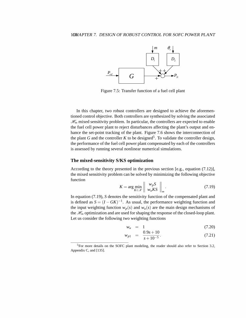
116CHAPTER 7. DESIGN OF ROBUST CONTROL FOR SOFC POWER PLANT
1D 2D
G fcPrefP
m sθ
Figure 7.5: Transfer function of a fuel cell plant
In this chapter, two robust controllers are designed to achieve the aforemen-tioned control objective. Both controllers are synthesized by solving the associatedH∞ mixed sensitivity problem. In particular, the controllers are expected to enablethe fuel cell power plant to reject disturbances affecting the plant’s output and en-hance the set-point tracking of the plant. Figure 7.6 shows the interconnection ofthe plantG and the controllerK to be designed5. To validate the controller design,the performance of the fuel cell power plant compensated by each of thecontrollersis assessed by running several nonlinear numerical simulations.
The mixed-sensitivity S/KS optimization
According to the theory presented in the previous section [e.g., equation (7.12)],the mixed sensitivity problem can be solved by minimizing the following objectivefunction
K = arg minK∈K
∥∥∥∥
wpSwuKS
∥∥∥∥
∞. (7.19)
In equation (7.19),Sdenotes the sensitivity function of the compensated plant andis defined asS= (I −GK)−1. As usual, the performance weighting function andthe input weighting functionwp(s) andwu(s) are the main design mechanisms oftheH∞ optimization and are used for shaping the response of the closed-loop plant.Let us consider the following two weighting functions
wu = 1 (7.20)
wp1 =0.9s+10s+10−5 . (7.21)
5For more details on the SOFC plant modeling, the reader should also referto Section 3.2,Appendix C, and [135].
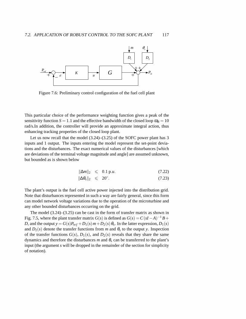
7.2. APPLICATION OF ROBUST CONTROL TO THE SOFC PLANT 117
ue
1D 2D
GK fcPrefP
m sθ
Figure 7.6: Preliminary control configuration of the fuel cell plant
This particular choice of the performance weighting function gives a peakof thesensitivity functionS= 1.1 and the effective bandwidth of the closed loopωB = 10rad/s.In addition, the controller will provide an approximate integral action, thusenhancing tracking properties of the closed loop plant.
Let us now recall that the model (3.24)–(3.25) of the SOFC power plant has 3inputs and 1 output. The inputs entering the model represent the set-point devia-tions and the disturbances. The exact numerical values of the disturbances [whichare deviations of the terminal voltage magnitude and angle] are assumed unknown,but bounded as is shown below
‖∆m‖2 6 0.1 p.u. (7.22)
‖∆θs‖2 6 20. (7.23)
The plant’s output is the fuel cell active power injected into the distribution grid.Note that disturbances represented in such a way are fairly general, since this formcan model network voltage variations due to the operation of the microturbine andany other bounded disturbances occurring on the grid.
The model (3.24)–(3.25) can be cast in the form of transfer matrix as shown inFig. 7.5, where the plant transfer matrixG(s) is defined asG(s) =C(sI−A)−1B+D, and the outputy= G(s)Pre f +D1(s)m+D2(s)θs. In the latter expression,D1(s)andD2(s) denote the transfer functions fromm andθs to the outputy. Inspectionof the transfer functionsG(s), D1(s), andD2(s) reveals that they share the samedynamics and therefore the disturbancesm andθs can be transferred to the plant’sinput (the argumentswill be dropped in the remainder of the section for simplicityof notation).
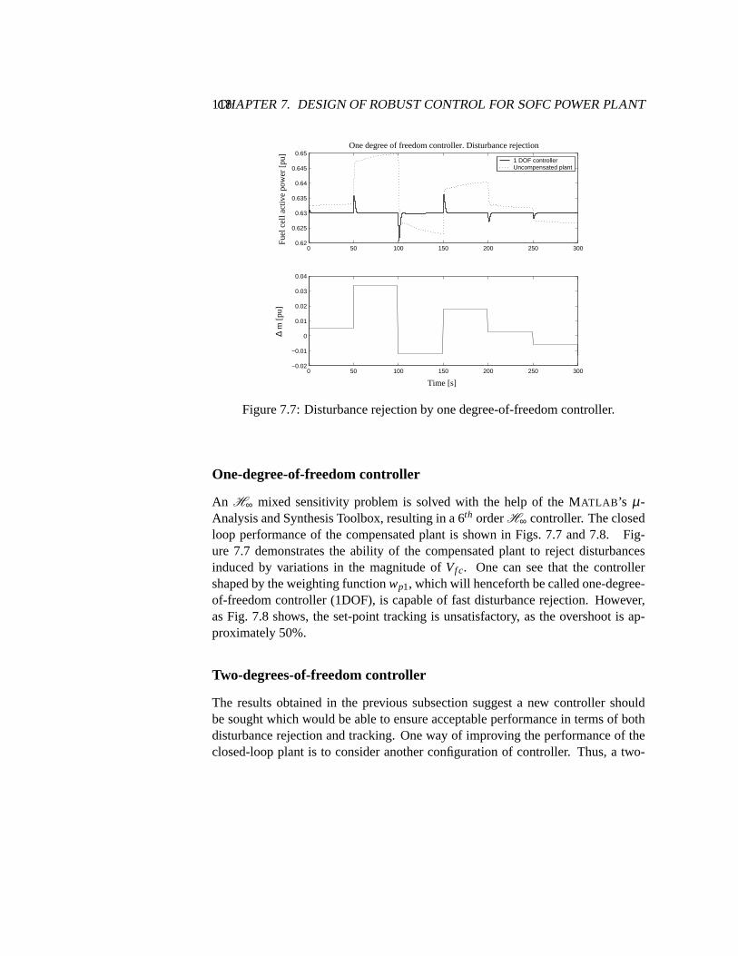
118CHAPTER 7. DESIGN OF ROBUST CONTROL FOR SOFC POWER PLANT
0 50 100 150 200 250 300−0.02
−0.01
0
0.01
0.02
0.03
0.04
Time [s]
∆ m
[pu]
0 50 100 150 200 250 3000.62
0.625
0.63
0.635
0.64
0.645
0.65One degree of freedom controller. Disturbance rejection
Fue
l cel
l act
ive
pow
er [p
u]
1 DOF controllerUncompensated plant
Figure 7.7: Disturbance rejection by one degree-of-freedom controller.
One-degree-of-freedom controller
An H∞ mixed sensitivity problem is solved with the help of the MATLAB ’s µ-Analysis and Synthesis Toolbox, resulting in a 6th orderH∞ controller. The closedloop performance of the compensated plant is shown in Figs. 7.7 and 7.8. Fig-ure 7.7 demonstrates the ability of the compensated plant to reject disturbancesinduced by variations in the magnitude ofVf c. One can see that the controllershaped by the weighting functionwp1, which will henceforth be called one-degree-of-freedom controller (1DOF), is capable of fast disturbance rejection. However,as Fig. 7.8 shows, the set-point tracking is unsatisfactory, as the overshoot is ap-proximately 50%.
Two-degrees-of-freedom controller
The results obtained in the previous subsection suggest a new controller shouldbe sought which would be able to ensure acceptable performance in terms of bothdisturbance rejection and tracking. One way of improving the performanceof theclosed-loop plant is to consider another configuration of controller. Thus, a two-
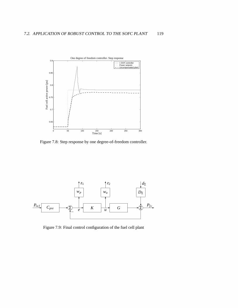
7.2. APPLICATION OF ROBUST CONTROL TO THE SOFC PLANT 119
0 50 100 150 200 250 300
0.65
0.7
0.75
0.8
0.85
0.9One degree of freedom controller. Step response
Fue
l cel
l act
ive
pow
er [p
u]
Time [s]
1 DOF controllerPower setpointUncompensated plant
Figure 7.8: Step response by one degree-of-freedom controller.
GCpre
wu
Σ
wp
-
DΣ
Σ K?- -
6
-
6
-Pre f
6 6?
6
-– e
z1 z2 dΣ
Pf cu
Figure 7.9: Final control configuration of the fuel cell plant
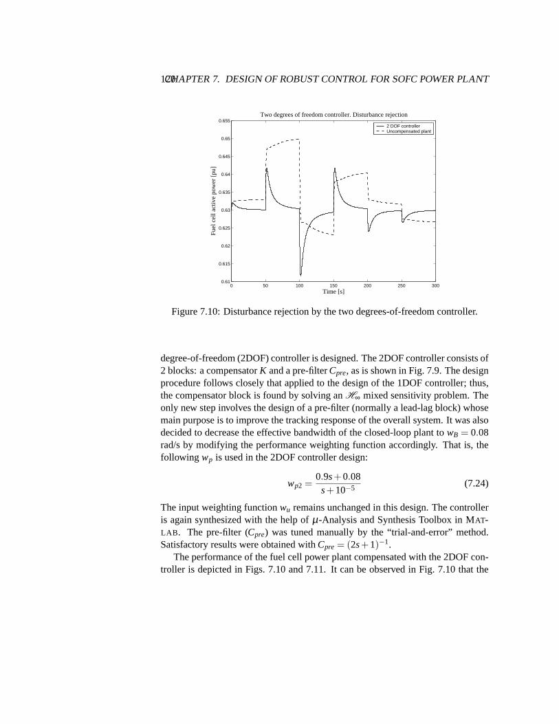
120CHAPTER 7. DESIGN OF ROBUST CONTROL FOR SOFC POWER PLANT
0 50 100 150 200 250 3000.61
0.615
0.62
0.625
0.63
0.635
0.64
0.645
0.65
0.655Two degrees of freedom controller. Disturbance rejection
Fue
l cel
l act
ive
pow
er [p
u]
Time [s]
2 DOF controllerUncompensated plant
Figure 7.10: Disturbance rejection by the two degrees-of-freedom controller.
degree-of-freedom (2DOF) controller is designed. The 2DOF controller consists of2 blocks: a compensatorK and a pre-filterCpre, as is shown in Fig. 7.9. The designprocedure follows closely that applied to the design of the 1DOF controller;thus,the compensator block is found by solving anH∞ mixed sensitivity problem. Theonly new step involves the design of a pre-filter (normally a lead-lag block) whosemain purpose is to improve the tracking response of the overall system. It was alsodecided to decrease the effective bandwidth of the closed-loop plant towB = 0.08rad/s by modifying the performance weighting function accordingly. That is, thefollowing wp is used in the 2DOF controller design:
wp2 =0.9s+0.08s+10−5 (7.24)
The input weighting functionwu remains unchanged in this design. The controlleris again synthesized with the help ofµ-Analysis and Synthesis Toolbox in MAT-LAB . The pre-filter (Cpre) was tuned manually by the “trial-and-error” method.Satisfactory results were obtained withCpre = (2s+1)−1.
The performance of the fuel cell power plant compensated with the 2DOF con-troller is depicted in Figs. 7.10 and 7.11. It can be observed in Fig. 7.10 thatthe
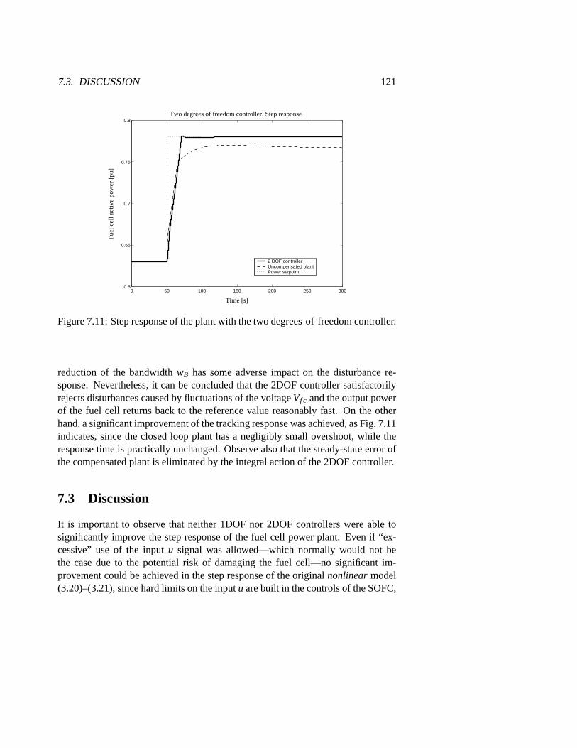
7.3. DISCUSSION 121
0 50 100 150 200 250 3000.6
0.65
0.7
0.75
0.8Two degrees of freedom controller. Step response
Fue
l cel
l act
ive
pow
er [p
u]
Time [s]
2 DOF controllerUncompensated plantPower setpoint
Figure 7.11: Step response of the plant with the two degrees-of-freedom controller.
reduction of the bandwidthwB has some adverse impact on the disturbance re-sponse. Nevertheless, it can be concluded that the 2DOF controller satisfactorilyrejects disturbances caused by fluctuations of the voltageVf c and the output powerof the fuel cell returns back to the reference value reasonably fast. On the otherhand, a significant improvement of the tracking response was achieved,as Fig. 7.11indicates, since the closed loop plant has a negligibly small overshoot, while theresponse time is practically unchanged. Observe also that the steady-stateerror ofthe compensated plant is eliminated by the integral action of the 2DOF controller.
7.3 Discussion
It is important to observe that neither 1DOF nor 2DOF controllers were abletosignificantly improve the step response of the fuel cell power plant. Even if“ex-cessive” use of the inputu signal was allowed—which normally would not bethe case due to the potential risk of damaging the fuel cell—no significant im-provement could be achieved in the step response of the originalnonlinearmodel(3.20)–(3.21), since hard limits on the inputu are built in the controls of the SOFC,
122CHAPTER 7. DESIGN OF ROBUST CONTROL FOR SOFC POWER PLANT
as follows from (3.21). The presence of the limits in the model is justified bythe necessity to avoid under- or over-utilization of the fuel cell, which is mainlyaccomplished by limiting the currentI r
f c of the fuel cell.The response time of a SOFC is limited by the time constants of the fuel proces-
sor, which are normally large and cannot be made smaller for a given fuelcell plantdue to physical limitations imposed by the parameters of the corresponding chem-ical reactions. Therefore, the response time of the plant cannot be enhanced bymanipulating its input, technological change in the fuel cell plant are required ifthe fuel cell power plant is to operate in a stand alone mode which requires load-following capabilities. Alternatively, other technical solutions should be sought;for example, the combined use of fuel cell modules and a gas turbine, or theuseof an external energy storage, such as batteries, a flywheel, or a superconductingmagnetic energy storage device.
Another alternative could be the use of a phosphoric acid fuel cell (PAFC)power plant which possesses significantly better load following capabilities.Forinstance, the commercial PAFC PC-25 according to [9]: “can be ramped at10kW/s up or down in the grid connected mode. The ramp rate for the grid indepen-dent mode is idle to full power in approximately one cycle or essentially one-stepinstantaneous from idle to 200 kW (nominal power). Following the initial rampto full power, the unit can adjust at an 80 kW/s ramp up or down in one cycle.”It should however be mentioned that the efficiency of PAFC plants is somewhatsmaller than that of SOFC/GT power plants.
7.4 Summary
In this chapter, a linearized model of a solid oxide fuel cell power plant was ob-tained. The linear model was used in order to design robust controllers capable ofrejecting disturbances caused by fluctuations of the magnitude and/or angleof theSOFC terminal voltage, which could in real world applications be caused by eitherthe fluctuation of the utility voltage (e.g., due to faults) or by the operation of themicroturbines. TwoH∞ controllers were synthesized and their performance wasanalyzed. To validate the performance of the controllers, nonlinear simulations ofa SOFC were performed. The load following capabilities of various fuel cell powerplants were briefly discussed. Apparently, further research in this area should in-volve numerical experiments with a more realistic model of the distribution gridand microturbines in order to assess the impact of the microturbine dynamics onthe operation of the solid oxide fuel cell power plant.
Chapter 8
Interaction Between DG and thePower System: Operation,Control, and Stability Aspects
“With so much new distributed generation beinginstalled, it is critical that the power system
impacts be assessed accurately.”— A quotation from [21]
This chapter presents qualitative analysis of the impact that distributed generation(DG) might have on the operation, control, and stability of electric power networkswith large penetration ratios. The impact of DG on network losses, power quality,short circuit power, as well as on system protection and on power system stabilityis discussed. Based on the discussion, it can be concluded that the impact of DG toa large extent depends on the penetration level of DG in the distribution network aswell as on the type of DG technology, and mode of its operation. If DG is properlysized, sited, and selected in terms of technology, it can clearly provide benefits tocontrol, operation and stability of the power system. It should however benotedthat distribution networks have traditionally a rather inflexible design (e.g., a uni-directional power flow), which in principle can cause integration problemswithhigher DG penetration levels or different technologies. Nonetheless, those issuescan usually be solved by modifying the distribution network, including the controland/or operation approach, or by other technical means.
8.1 IntroductionSeveral technical, political, and environmental considerations have stimu-lated the relatively rapid growth of the number of various DG installations.While the total installed capacity of the distributed generation remained
small, its impact on the operation of the power grid remained marginal; however,
123

124CHAPTER 8. INTERACTION BETWEEN DG AND THE POWER SYSTEM
as the installed capacity of DG increases, the impact which it has on the grid willintensify. The characterization and quantification of this impact apparently isquitea complicated engineering task, since such aspects of grid operation as voltagecontrol, relay protection coordination, power losses, power quality, reliability, andmany other will have to be simultaneously analyzed. Some of these aspects arealso intimately related to the stability phenomena of the grid and therefore theywill have to be explicitly addressed in the studies of the overall power systemsta-bility.
To assist in making a systematic assessment of the impact that large amountsof DG have on the operation, control, and stability of the power grid, this chap-ter provides basic qualitative analysis of the interaction between large amounts ofdistributed generation and the power network.
8.2 Historical Background
The importance of the impact that DG might have on the operation, stability, andcontrol of the power system has already been recognized in the late 1970’s. Oneof the most interesting publications on this subject was presented at the conference“Research needs for the effective integration of new technologies into the ElectricUtility” held by the U.S. Department of Energy (DoE) in 1982 and was entitled“Impacts of new technology and generation and storage processes on power sys-tem stability and operability” [109]. Over the last two decades the number ofpublications discussing various areas of the interaction between DG and theutilityhas been gradually increasing. Historically, until the 1990’s the main focusof theresearch was placed upon the impact that renewable power sources had on networkoperation, [46], [99]; however, also distributed generation in general was inves-tigated [2]. In the late 1990’s, this theme gained more interest in academia andindustry, which resulted in a large number of publications [6,7,10,11].
Recently, also the results of two extensive simulation case studies have beenreported: (i) Simulation of interaction between wind farm and power system, by theRisø National Laboratory, Denmark [120], and (ii) DG Power Quality, Protectionand reliability Case Studies Report, by GE Corporate Research and Development,USA [97].

8.3. DISTRIBUTED GENERATION TECHNOLOGY 125
Table 8.1: Technologies for distributed generation [13].
Technology Typical available size p. module
1. Combined Cycle Gas T. 35−400MW2. Internal Combustion Engines 5kW−10MW3. Combustion Turbine 1−250MW4. Micro-Turbines 35kW−1 MW5. Small Hydro 1−100MW6. Micro Hydro 25kW−1 MW7. Wind Turbine 200W−3 MW8. Photovoltaic Arrays 20W−100kW9. Solar Thermal, Central Receiver 1−10MW10. Solar Thermal, Lutz System 10−80MW11. Biomass Gasification 100kW−20MW12. Fuel Cells, PhosAcid 200kW−2 MW13. Fuel Cells, Molten Carbonate 250kW−2 MW14. Fuel Cells, Proton Exchange 1−250kW15. Fuel Cells, Solid Oxide 250kW−5 MW16. Geothermal 5−100MW17. Ocean Energy 0.1−1 MW18. Stirling Engine 2−10kW19. Battery Storage 0.5−5 MW
8.3 Distributed Generation Technology
One of the most essential factors influencing the interaction between the DG andgrid is the technology utilized in the DG, as well as the mode of DG control andoperation.
Table 8.1 provides a brief overview of the most commonly used distributedgeneration technologies and their typical module size. The technologies 5− 11,16 and 17 can be considered renewable DG. The other technologies could alsobe called renewable DG if they are operated with biofuels. Also fuel cells couldbe considered renewable DG if the hydrogen is produced using renewable energysources, e.g. wind power.
Similarly to the centralized generation, the following three generation technolo-gies are normally used for distributed generation: synchronous generator, asyn-chronous generator, and power electronic converter interface [8,51,62,90]. These

126CHAPTER 8. INTERACTION BETWEEN DG AND THE POWER SYSTEM
DG technologies will now be briefly discussed.
Synchronous Generator
The advantageous ability of the synchronous generator—the primary generatortechnology for centralized generation—to produce both active and reactive poweralso provides benefits for distributed generation applications.
Synchronous generators are typically utilized by the following DG applicationsif the generation capacity exceeds a few MW: biomass, geothermal, diesel/gas en-gines driven generators, solar thermal generation, solar parabolic systems, solarpower towers, solar dish engines, gas turbines, and combined cycle gasturbines.
Asynchronous Generator
In contrast to synchronous generators, asynchronous (induction)generators areonly used for distributed generation, but not for centralized generation. An asyn-chronous generator is basically an induction machine which is connected to aprime-mover. When the generator is connected to the power network, the mechan-ical power is converted into electrical power by the action of the prime-moverthatdrives the machine above synchronous speed. Hence, the asynchronous generatoris not capable of operating independent from a relatively strong grid. Asynchro-nous generators are used for many distributed generation technologies as long asthe generation capacity does not exceed a few MW due to its competitive pricecompared to synchronous generators. Squirrel cage asynchronous generator usedto be very common in the wind energy industry; however, this type of inductiongenerator is now being gradually superseded by asynchronous generators equippedwith a converter, i.e., double-fed induction generators.
Power Electronic Converter
Power converters normally use high power electronics to provide the desired poweroutput. For example, it is quite common that wind turbines use double-fed, variablespeed induction generators with an IGBT converter in the rotor circuit. Power elec-tronic converters are also used in photovoltaic systems, fuel cells, micro turbines,Sterling engine as well as battery storage, and magnetic storage systems.
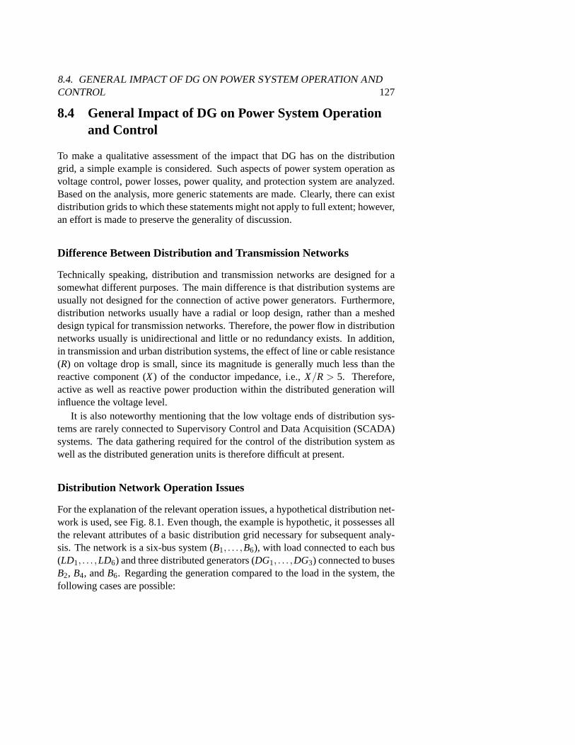
8.4. GENERAL IMPACT OF DG ON POWER SYSTEM OPERATION ANDCONTROL 127
8.4 General Impact of DG on Power System Operationand Control
To make a qualitative assessment of the impact that DG has on the distributiongrid, a simple example is considered. Such aspects of power system operation asvoltage control, power losses, power quality, and protection system are analyzed.Based on the analysis, more generic statements are made. Clearly, there canexistdistribution grids to which these statements might not apply to full extent; however,an effort is made to preserve the generality of discussion.
Difference Between Distribution and Transmission Networks
Technically speaking, distribution and transmission networks are designedfor asomewhat different purposes. The main difference is that distribution systems areusually not designed for the connection of active power generators. Furthermore,distribution networks usually have a radial or loop design, rather than a mesheddesign typical for transmission networks. Therefore, the power flow in distributionnetworks usually is unidirectional and little or no redundancy exists. In addition,in transmission and urban distribution systems, the effect of line or cable resistance(R) on voltage drop is small, since its magnitude is generally much less than thereactive component (X) of the conductor impedance, i.e.,X/R > 5. Therefore,active as well as reactive power production within the distributed generation willinfluence the voltage level.
It is also noteworthy mentioning that the low voltage ends of distribution sys-tems are rarely connected to Supervisory Control and Data Acquisition (SCADA)systems. The data gathering required for the control of the distribution system aswell as the distributed generation units is therefore difficult at present.
Distribution Network Operation Issues
For the explanation of the relevant operation issues, a hypothetical distribution net-work is used, see Fig. 8.1. Even though, the example is hypothetic, it possesses allthe relevant attributes of a basic distribution grid necessary for subsequent analy-sis. The network is a six-bus system (B1, . . . ,B6), with load connected to each bus(LD1, . . . ,LD6) and three distributed generators (DG1, . . . ,DG3) connected to busesB2, B4, andB6. Regarding the generation compared to the load in the system, thefollowing cases are possible:
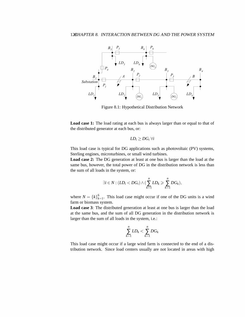
128CHAPTER 8. INTERACTION BETWEEN DG AND THE POWER SYSTEM
DG1
P1
P2 P
3
Substation
LD1
LD2
LD3
LD4
A BB1
B2
B3
B4
P4
DG3
P5
P6
LD5
LD6
B5
B6
DG2
Figure 8.1: Hypothetical Distribution Network
Load case 1:The load rating at each bus is always larger than or equal to that ofthe distributed generator at each bus, or:
LDi ≥ DGi ∀i
This load case is typical for DG applications such as photovoltaic (PV) systems,Sterling engines, microturbines, or small wind turbines.Load case 2:The DG generation at least at one bus is larger than the load at thesame bus, however, the total power of DG in the distribution network is less thanthe sum of all loads in the system, or:
∃i ∈ N : (LDi < DGi)∧ (n
∑k=1
LDk >n
∑k=1
DGk),
whereN = k6k=1. This load case might occur if one of the DG units is a windfarm or biomass system.Load case 3: The distributed generation at least at one bus is larger than the loadat the same bus, and the sum of all DG generation in the distribution network islarger than the sum of all loads in the system, i.e.:
n
∑k=1
LDk <n
∑k=1
DGk
This load case might occur if a large wind farm is connected to the end of a dis-tribution network. Since load centers usually are not located in areas with high

8.4. GENERAL IMPACT OF DG ON POWER SYSTEM OPERATION ANDCONTROL 129
?
SDG
SLD
6
V
R+ jX
E
Figure 8.2: Simplified model of a power system with DG
wind speeds, the power output of a wind farm often can exceed the localpowerdemand. Finally, it must be mentioned that the load cases within a distribution net-work might change over time. It is, for example, quite common that a wind farmprovides a significant amount of the load in a distribution network for most ofthetime (Load case 2). The other two load cases, however, can also occur.Load case1 during times with little wind and load case 3 during times with very high windspeeds and low loads, for example, during the night.
Impact on Losses
To explain the impact of DG on distribution network operation under considerationof differentX/R ratios, the simplest model—a single distribution line and a load—is used.
In the model presented in Fig. 8.2,E represents the sending end voltage,V isthe receiving end voltage. If we assume that the receiving voltageV as well as theload currentI are known, then the following equations establish the relationshipbetween the power produced by DG and associated reduction of losses on the line.Suppose no DG is connected. Then the power losses are
Sloss= (E−V)I∗ = (E−V)(ILD,a− jILD,r),
whereILD,a andILD,r denote the active and reactive components of the load current.Now assume that DG producing only active power (cosφ = 1) is connected andalso assume for simplicity that the voltageV at the receiving end is kept constant.Then it is easy to see that the new power losses are:
SDGloss= (E−V)(ILD,a− IDG− jILD,r).
130CHAPTER 8. INTERACTION BETWEEN DG AND THE POWER SYSTEM
Therefore, the presence of DG reduces the power loss by the amount
Sloss−SDGloss= (E−V)IDG.
With this approximate expression, the variations of the voltage at the receiving endare not considered; however, the inclusion of the receiving voltage variations is notessential for the analysis. In summary, it can be concluded that the introductionof distributed generation reduces the current flowing through the distribution line,thus reducing the active as well as reactive power losses.
Based on three load cases defined at the beginning of this section, the followingcan be said:
Load case 1DG will always result in reduced losses on all lines in the distributionnetwork.
Load case 2DG might lead to an increase of the losses on some lines, but the totallosses within the [realistic] distribution network will be reduced.
Load case 3DG might lead to an increase of the losses on some lines, but the totallosses within the [realistic] distribution network will be reduced as long asthe total DG production is less than approximately twice the total load in thedistribution network.
If the DG production is larger than approximately twice the total load in the distri-bution network, the losses in the distribution network will be larger with DG con-nected than without DG. In addition, it should be noted that a power loss reductionin the distribution network entails a loss reduction in the transmission network.
Voltage Control
The voltage level in a distribution network must be kept within a certain range,assome power system equipment and customer applications function only properly ifthe voltage is maintained within this range. The voltage range for normal operationis defined in different national and international standards.
In a distribution system voltage fluctuations occur when the load current flow-ing through the resistive and reactive impedances of the lines varies. Thevoltagevariations in distribution networks without DG are caused by the variations oftheactive and reactive load in the distribution network over time. The fluctuationsare generally larger towards the end of the line, due to the high impedance ofdis-tribution lines. Also, the voltage fluctuations are more expressed if the load is
8.4. GENERAL IMPACT OF DG ON POWER SYSTEM OPERATION ANDCONTROL 131
concentrated near the end of the (radial) system. Practically, for typical distribu-tion lines the distance before the voltage drop exceeds the allowable fluctuation atrated current is only a few km. However, a line is normally not designed to operateat such loading levels. An in-depth analytical discussion of the impact of DGonthe voltage profile in LV networks can be found in [32].
Traditionally, voltage control in distribution networks is performed in two ways:
1. The control of the source voltage at the network substation by using tapchanging transformers and;
2. The control of the reactive power throughout the system, by using shuntcapacitors/shunt reactors [this is very seldom done in distribution networks],series capacitors, synchronous condenser or Static VAr Compensator(SVC).
DG can influence the voltage variations in two ways:(i) DG is operated in correlation with the local load requirements, meaning when-ever the local load in the distribution network increases, the DG production in-creased as well, and vise versa. In this case, DG contributes to the reduction of thevariations between the maximum and minimum voltage levels, compared to thesituation without DG. This mode of DG operation provides no challenges to thetraditional voltage control approach. This situation was thoroughly investigatedin [77]. This DG control mode is well suited for photovoltaic distributed genera-tors, if the local loading [e.g., air conditioning equipment] is naturally correlatedto the solar radiation and thus the power output of the photovoltaic cells.(ii ) DG power output is controlled independently of the local loading of the area.This control mode is implemented if DG operation follows price signals, whichmight or might not correspond to the local load variations, or DG follows the avail-ability of natural resources, like solar or wind power. In this case, DG might ad-versely affect the voltage control functionality of the network by increasing thevariations between the maximum and minimum voltage level, compared to a situa-tion without DG, since the minimum voltage level could remain (usually at a highload, no DG situation) but the maximum voltage level could increase, e.g. in lowload situations with DG operating at maximum production and at a unity powerfactor. Generally speaking, DG can provide some challenges to the traditionalvoltage control. For example, during a high load situation in the hypothetical net-work shown in Fig. 8.1, the tap changing transformer (not shown) at the substationwould increase the source voltage to keep the voltage at the end of the lines (busB4
and busB6) within the required voltage range. Now with a large DG unit at busB6,but no DG at busB4, the voltage at busB6 is raised due to DG and might reach the
132CHAPTER 8. INTERACTION BETWEEN DG AND THE POWER SYSTEM
overvoltage limits, while the voltage at busB4 could reach the lower voltage limitsdue to the high load. The traditional operation approach of tap changing trans-former at the substation is not suitable for such situation, as it assumes a similarvoltage drop on all lines downstream from the transformer.
One simple approach to solve this problem is to reduce the power output of theDG unit. This solution will be the most economic solution for the network operatorbut probably not for the DG owner. In case of intermittent renewable generation,particular wind power, there is a low likelihood that the maximum availability ofthe natural resources, e.g. very high wind speeds, correlates with very low loadsituation. On the Swedish island of Gotland, for example, such a situation occursaround 10 hours per year. Another, more costly solution would be the installationof a more intelligent and flexible voltage control scheme within the distributionsystem, based on substation automation and modern communication technology.This technology would allow sensing the voltage level at different points in thenetwork, usually at the end of different lines. Hence, the tap changer setting atthe substation could be dynamically adjusted according to the input data from themeasurements. In addition, if the applied DG technology has the capability of dy-namically changing the power factor it could be used to locally control the voltage.The aim would be to keep the voltage variations in the distribution network withintolerable limits. This is already done within some wind power projects, wherethe power electronic converter is used for dynamic voltage control in the distri-bution system [31]. In general, DG technologies using either a power electronicsconverter [114] or a synchronous generator could be used for dynamic voltage con-trol. The approach, however, is rather seldom used—the author is only aware of 3projects worldwide—due to the following two reasons:(i) Interconnection rules usually do not allow an active participation in the controlof the distribution network. This might change with the new IEEE Standard forDistributed Resources Interconnected with Electric Power Systems, which iscur-rently under discussion. A change of the interconnection rules still leavesopenquestions: What is the economic value of dynamic voltage control with DG, orin other words: How much must the network operator pay the DG operator forthe voltage control service. In most projects where DG current provides dynamicvoltage control, the service was requested by the network operator.(ii ) If DG provides active voltage control the remaining voltage control system,for example tap changer or capacitor banks, might have to be coordinatedwiththe DG voltage control system to avoid voltage hunting. Voltage control results infast change of voltage level in the distribution system due to interaction betweendifferent voltage control systems. The coordination between the different voltage

8.4. GENERAL IMPACT OF DG ON POWER SYSTEM OPERATION ANDCONTROL 133
control systems could be done with the help of modern communication systems.
Power Quality
When discussing the impact of DG on power quality, there are typically two majorconcerns, namely, voltage flicker and harmonics.
Voltage Flicker
As defined in [37], voltage flicker is an impression of unsteadiness of visual sen-sation induced by a light stimulus whose luminance or spectral distribution fluc-tuates with time. In distribution networks the most common cause of flicker is arapid variation of load current. However, not only load variations causeflicker, butalso DG can directly or indirectly contribute to voltage flicker. The main causesofflicker are
(i) Starting of a large DG unit
(ii) Sudden and large variations of the output of DG
(iii) Interactions between DG and the voltage controlling equipment of the feeder.
Voltage flicker mitigation method and its effectiveness depend on many factorsandcan be quite complicated. If the rating of DG is significant and the output of DGissubject to frequent and significant change, then voltage flicker may be felt by somecustomers. The simplest mitigation method in such a case would be to require theowner of DG to reduce the number of DG starts and/or large variation of the outputpower. If DG is interfaced with the grid via a converter, then reduction of startingcurrents is relatively easy to accomplish. In particular, wind farms have been seenas potential cause of voltage flicker due to wind speed variations or poweroutputvariation due to passage of the wind turbine blades through the tower shadow.However, the design of modern wind turbines has been changed such that largevariations of the output power within a short time period can be effectively avoided(variable speed).
Harmonics
It is widely recognized that the presence of nonlinear components of power sys-tems, e.g., power converters or saturated transformers, manifests in the appearanceof harmonics [37]. The presence of harmonics in a power system is undesirable fora number of reasons, some of which are:
134CHAPTER 8. INTERACTION BETWEEN DG AND THE POWER SYSTEM
(i) Harmonics increase power loss in both utility and customer equipment
(ii) Sometimes harmonics may provoke malfunctioning of sensitive load or controlequipment [86]
(iii) Harmonics having significant magnitudes can cause a reduction of lifetime ofmotors, transformers, capacitor banks, and some other equipment.
Power electronic devices, as used for DG, might cause harmonics. The magni-tude and the order of harmonic currents injected by dc/ac converters depend onthe technology of the converter and the mode of its operation. For example, aforced-commutated converter with pulse-width-modulation operated in the linearrange, will introduce only harmonics in the range of high frequencies, i.e.,at and/oraround multiples of the carrier frequency [85]. Recent advances in semiconductortechnology (e.g. IGBT’s) allow the use of higher carrier frequencies;which, forexample, allows the generation of quite clean current waveform in compliantwiththe IEEE 519 standard. IGBT based converter are used for many DG technologies.It can therefore be concluded that modern high power electronics technology canbe used to solve the relevant power quality phenomena associated with DG.
Voltage Sags
Theoretically, distributed generation based on power converters can beused to re-duce the depth of voltage sags. In this case, the converter must act as a static VArcompensator or dynamic voltage restorer. In principle, power electronic convertercan be designed to operate in those modes; however, presently most of distrib-uted generation converters seem to be incapable of performing this task. Abasicrequirement is that the distributed generation system has sufficient capacity to com-pensate for the utility voltage reduction and maintain acceptable voltage level forthe duration of the voltage sag. As is stated in [37], the improvement of powerqual-ity in respect to voltage sags by using distributed generation is “a good function toconsider in the future”. In quasi-stationary operation the qualitative impactof dis-tributed generation on voltage magnitude is practically indistinguishable from thatof a large [negative] load. Indeed, switching of a large load causes voltage magni-tude variations, which is similar to the effect that DG output power variation has.The output power variations of a large load and a distributed generator utilizingrenewable energy source e.g. wind or solar energy are subject to dailyand seasonalvariations. On the other hand, in many respects DG affects power quality ofthegrid in a very specific way. For example, the owner of a distributed generator—if the DG technology allows—has full control of the output power and voltage
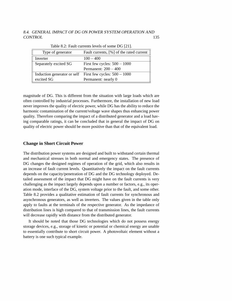
8.4. GENERAL IMPACT OF DG ON POWER SYSTEM OPERATION ANDCONTROL 135
Table 8.2: Fault currents levels of some DG [21].
Type of generator Fault currents, [%] of the rated current
Inverter 100−400Separately excited SG First few cycles: 500−1000
Permanent: 200−400Induction generator or self First few cycles: 500−1000excited SG Permanent: nearly 0
magnitude of DG. This is different from the situation with large loads which areoften controlled by industrial processes. Furthermore, the installation of new loadnever improves the quality of electric power, while DG has the ability to reduce theharmonic contamination of the current/voltage wave shapes thus enhancing powerquality. Therefore comparing the impact of a distributed generator and a load hav-ing comparable ratings, it can be concluded that in general the impact of DGonquality of electric power should be more positive than that of the equivalentload.
Change in Short Circuit Power
The distribution power systems are designed and built to withstand certain thermaland mechanical stresses in both normal and emergency states. The presence ofDG changes the designed regimes of operation of the grid, which also results inan increase of fault current levels. Quantitatively the impact on the fault currentsdepends on the capacity/penetration of DG and the DG technology deployed. De-tailed assessment of the impact that DG might have on the fault currents is verychallenging as the impact largely depends upon a number or factors, e.g., itsoper-ation mode, interface of the DG, system voltage prior to the fault, and some other.Table 8.2 provides a qualitative estimation of fault currents for synchronous andasynchronous generators, as well as inverters. The values given inthe table onlyapply to faults at the terminals of the respective generator. As the impedanceofdistribution lines is high compared to that of transmission lines, the fault currentswill decrease rapidly with distance from the distributed generator.
It should be noted that those DG technologies which do not possess energystorage devices, e.g., storage of kinetic or potential or chemical energy are unableto essentially contribute to short circuit power. A photovoltaic element withoutabattery is one such typical example.
136CHAPTER 8. INTERACTION BETWEEN DG AND THE POWER SYSTEM
Protection System
By definition, protective relays and systems are power system componentswhichshould “operate the correct circuit breakers so as to disconnect onlythe faultyequipment from the system as quickly as possible, thus minimizing the trouble anddamage caused by faults when they do occur” [125]. There are a number of powersystem protection devices whose functionality ranges from overcurrent protectionto bus-zone protection [17]. The section will focus on overcurrent protection, themost commonly used protection in distribution systems. As mentioned before, thepower flow in distribution systems is usually in one direction-from the source tothe customers. Correspondingly, the protection schemes of distributions grids aredesigned for this mode of operation. The presence of DG may alter the topology ofthe distribution grid and the pattern of the power flow. Depending on the charac-teristics of DG (its rated power, technology used, mode of operation), the locationof DG and network configuration, the impact of DG on the overcurrent protec-tion may vary. To exemplify the statement, consider the distribution grid shown inFig. 8.1. Normally, the protection of power systems is tuned in such a way that onlyfaulted parts of the system are isolated at a fault. This tuning is termed “protectioncoordination.” Suppose now that all the DG units is disconnected from the gridand a fault located atB occurs on the system, see Fig. 8.1. The overcurrent pro-tection coordination assures that the protection deviceP3 reacts, thereby avoidingmuch interruption of power delivery to the other customers. Alternatively, supposethat DG is now connected to the grid. Clearly, under some operating conditionsthe power on the lines may flow either downstream or upstream. This has cer-tain implications on the operation of the protection schemes. Assume again a faultlocated atB. Then the short circuit current flowing through the protection deviceP3 is greater than that of the deviceP2. On the other hand, if a fault located atAis encountered, the fault current ofP2 is greater than the current flowing throughdeviceP3. This example clearly indicates that DG will certainly impact the protec-tion scheme of the distribution grid. More examples similar to this can be foundin [44]. There are at least two solutions to the problem described above.Appar-ently, the simplest solution is to require all DG units be disconnected when a faultoccurs on the grid. This is the current practice for most DG interconnections. If theprotection system of DG units are able to detect the fault and rapidly disconnectfrom the network, DG will not interfere with the normal operation of the protectionsystem. Most interconnection standards therefore require disconnection of DG if afault occurs. However, this is not always desired, particular when DGpenetrationis high in a distribution network. Nowadays, more and more distribution networks

8.4. GENERAL IMPACT OF DG ON POWER SYSTEM OPERATION ANDCONTROL 137
are automated and equipped with SCADA systems. The primary objective of thesesystems is to improve reliability of the grid, but they can also be helpful in dynamiccoordination of the system protection relays. In brief, a SCADA system might al-low the coordinated control of the protection system, by analyzing the relevantdata (system voltages, level of loading, the DG production, etc.) and operating thereclosers/circuit breakers that would isolate the fault without much disturbance toother customers or unnecessary disconnection of DG.
Reliability
The assessment of impacts that DG might have on the grid is complicated by sev-eral considerations, including the following ones
• Main application of DG.
• Plans concerning the future development of the grid.
• The technology of DG.
Combination of the aforementioned factors determines the overall impact that DGcan have on the system reliability. Let us examine qualitatively these factors.Tosimplify analysis, let us only consider distributed generators with fully control-lable output power. That is, such DGs as photovoltaic arrays or wind turbines areleft outside the scope of the analysis. According to [26], there are threemain ap-plications of DG, namely, providing back up power, peak load shaving, and netmetering. It can be argued that the impact of DG on the overall system reliabilitydepends on the application. For instance, DG installed with the purpose to provideback up power will certainly increase the reliability of power supply to the criticalload it is protecting. However, the positive impact on the reliability of the powerdelivery to other customers will be only marginal. Positive impacts that DG canhave on the grid are more expressed when the main aim of the DG is to reducethe peak power demand. The positive impact originates from the fact that electricpower is generated and consumed on-site thereby unloading the main feeder, whichis likely to increase the overall system reliability due to a reduced rate of failureson the distribution grid.
The impact of net metering on the overall system reliability can be two-fold.On the one hand, net metering may contribute to peak load shaving and thus en-hance reliability of power delivery. On the other hand, this application, in principle,causes bidirectional power flows, which under certain circumstances can depressreliability of the grid. In addition, the presence of such distributed generators can
138CHAPTER 8. INTERACTION BETWEEN DG AND THE POWER SYSTEM
mask the load growth and therefore increase the number of customers whichcanbe affected by power interruption due to a failure of the DG. For instance,if a dis-tributed generator is installed in the middle of a feeder, then at the substation end ofthe feeder an increase of the load behind the DG may be difficult to recognize. Thismight lead to an increased number of customers affected by a fault on the feeder orthe DG itself. In conclusion it can be stated that major impacts that DG can haveon the system reliability is highly dependent on the DG characteristics, grid char-acteristics as well as the application of DG. The same DG technology utilized fordifferent applications will affect system reliability in different ways, ranging fromvery positive impact (peak load shaving) to quite negative (load growth masking,changing the load flow pattern). A more detailed treatment of the impact of distrib-uted generation on the power grid and methods useful for quantifying the impactcan be found in [26]. It must however be stated that “despite these conflicts, DGinstallations on utility distribution systems can nearly always be successfully engi-neered” [37].
8.5 Network Control and Stability Issues
The following sections will briefly discuss what impact a significant penetration ofDG might have on control and stability of power systems. Within the discussionabout DG and control/stability issue often the question about a critical penetrationlevel of DG emerges. In the author’s opinion, the critical penetration leveldoesnot necessarily have to be defined as it will depend on the network designandthe technology used, if there is actually any critical penetration level for DG. Itis sometimes speculated in the literature on DG that distributed generators willcertainly lead to control and stability issues. In what follows an attempt is madeto qualitatively show thatin generalsuch a statement cannot be made, at leastfor relatively small penetration levels. The discussion in this section echoestheconclusions from the previous chapters in this thesis; however, an attemptis madeto extrapolate these conclusions to a general multimachine power system, which—at present—can only be done by performing basic qualitative analysis.
Islanding
A loss-of-main or islanding problem can occur if a circuit breaker in a distributionsystem opens, which could results in an islanding of a DG unit. If the loss-of-mainis not detected by the DG unit, for example due to insufficient fault current,the DGunit will continue to operate. If the DG unit is able to match active and reactive
8.5. NETWORK CONTROL AND STABILITY ISSUES 139
power of the load in the islanded system precisely, then the islanded system couldcontinue to operate. In this case a safety issue remains, as the network staff mightassume that the islanded network is not energized. It is, however, veryunrealis-tic that DG will exactly match the load in the system during the time the circuitbreaker opens, hence large frequency or voltage variations will occur when the DGunit tries to supply load. Hence, most interconnection rules require a loss-of-maindetection system which automatically disconnects the DG unit in case of a loss-of-main and the unit remains disconnect until the grid is restored. In the UK,G59recommendations requires that all DG units connected to MV or LV with a ratinggreater than 150 kVA have a loss-of-main detection system [63]. Apparently, manycustomers have an interest to operate DG in parallel to the network as long asthenetwork is available, but if a network outage occurs they would like to operate theDG unit as emergency power supply or back-up unit. In this case, the DG unit mustdisconnect from the main grid and must quickly match the local load demand.
Availability of Relevant Data
When analyzing stability of a power system, both dynamic and transient stabilityissues should be addressed in order to numerically assure the proper and reliableoperation. Be it dynamic or transient stability study, it is extremely important tohave models of the system reflecting the main dynamical features of the systemwith reasonable accuracy. Thus, to obtain reliable results from a study, one ulti-mately needs the data of the system components. This implies that the owners ofDG should make all relevant technical characteristics of DG available. Here, notonly the static characteristics of the DG unit are important, but also the character-istics of the main controls such as the governor, voltage regulator, and excitationsystem of a synchronous generator, etc. should be available.
Dynamic Models of DG Technologies
As the distribution grids are becoming more active their behavior will more resem-ble that of a transmission network. When the penetration level passes a certainthreshold it will no longer be appropriate to model the distribution networks asjust static loads characterized by the amount of active and reactive power beingconsumed. Just as in the case of the transmission grid, it will be necessaryto ac-curately model both the distributed generators and their loads in order to addresssuch issues as stability and control of DG resources. The importance of the mod-eling of the new DG technologies has already been realized by the researchers and
140CHAPTER 8. INTERACTION BETWEEN DG AND THE POWER SYSTEM
engineers and resulted in a number of scientific articles reporting the developmentof dynamic models of fuel cell systems, microturbines, double fed induction ma-chines, and generic loads [38,41,72,78,94,115–117,123,135]. Depending on thedynamical phenomena of interest, various models can be used in the analysisandsimulations; however, it should be noted that presently most of the commerciallyavailable power simulation packages do not have detailed models of such DG tech-nologies as a fuel cell or doubly-fed induction machines. Therefore, presently thesystem analyst has to face the challenge of modeling various components withoutrelying on the availability of well-established models. If for some reason analyticalmodeling is inaccurate or infeasible, alternative ways of obtaining reliable modelsshould be sought. One such solution is to apply a system identification technique.System identification techniques have proven useful and robust numerical tools forobtaining reliable models of dynamical systems in various fields of modern en-gineering, e.g., biomedicine, signal processing, aerospace industry and are nowgaining more momentum in power system applications. Certain results have al-ready been obtained in identification of linear and nonlinear models of fuel cellstack and an aggregate industrial load [72], [112]. In conclusion it can be statedthat the choice of the dynamic model to be used in a particular case strongly de-pends in the nature of the study. That is, when assessing the dynamic stabilityof apower system, linear models—possibly obtained with the help of a linear identifi-cation method—will suffice. When a linear system is obtained by linearization ofa nonlinear model, an explicit assumption is made on the magnitude of deviationsof the system’s states from an equilibrium point-the deviations should be smallfor all times. If this assumption is violated, the results from the linearized modelmay not be reliable. If this is the case, the use of linear tools becomes a choiceofquestionable value and application of nonlinear techniques should be consideredas a viable alternative. When studying transient stability issues in electric powersystems, nonlinear models are commonly used [88]. The necessity to model powersystems with nonlinear differential equations originates from the following fact:When a power system is subjected to a sudden and severe disturbance, itsstates(generators shaft angular frequencies, exciter voltages, etc.) may deviate signif-icantly from the pre-fault steady state. Moreover, a new post-fault equilibriummay be different from the pre-fault, which implies that linear models for pre-andpost-fault are also different. All these considerations suggest that nonlinear systemanalysis should be applied to a certain class of power system studies. There aremany nonlinear analysis tools that can be used for stability studies in power systemapplications. One of the most commonly used techniques is the Lyapunov directmethod and its modifications presented in Chapter 4 and [43,64,95].

8.5. NETWORK CONTROL AND STABILITY ISSUES 141
Change of Short Circuit Capacity
The installation of new distributed generators on the distribution networks poten-tially brings a number of benefits; however, it also may cause some side effects.One of those effects is the increased level of short circuit capacity (SCC) of thedistribution networks. Although sometimes it is desirable to have a high SCC, e.g.,at the point of connection of the inverter of a line commutated HVDC station or inthe presence of large loads with rapidly varying demands, in general the increaseof the SCC potentially indicates a problem. The problem is two-fold:
(i) Increased fault currents and
(ii) Voltage control issues.
Now these topics will be considered in more detail. To facilitate the exposition,assume a DG unit has been installed at a busbarA of an abstract distribution grid.Prior to the installation of DG, busbarA was a pure PQ node; with the distributedgenerator installed it becomes active and produces a certain amount of power at aconstant power factor. Suppose a fault occurred in a neighborhoodof busbarA. AsTab. 8.2 suggests, during a fault a distributed generator can inject into thebusbarfault currents of a magnitude ten times greater than its rated current. Such currentscan cause two types of problems: thermal and mechanical stress to the busbar.It is well known that the mechanical force acting on a busbar during a fault isproportional to the square of the fault current. In addition to the mechanical stressunder faulted conditions the busbar will also be exposed to thermal stress,whichcan also cause damage to the busbar. Another issue to be addressed in connectionwith the increase of SCC is the voltage control problem. If the voltage ofA atsteady state is 1 p.u., then after a sudden load level reduction the voltage of Amightincrease beyond the desirable limits. The presence of shunt capacitors and/or filtersinstalled to compensate for the reactive power or harmonics absorption may furtherworsen the situation. We would like however to mention that so far only the worstcase scenarios have been considered. In reality the situation might actuallybe lesssevere. That is, normally low voltage lines and cables do have resistance values ofa comparable magnitude with that of the reactance. Thus, the relative impedance[Ω/km] of the distribution lines is greater than that of transmission lines. Therefore,the fault currents will quickly dwindle as the distance betweenA and the faultincreases causing less or no damage toA.
It should be noticed that the overwhelming majority (up to 70–80%) of thefaults are one-phase-to ground and are of temporary character, which also reduces

142CHAPTER 8. INTERACTION BETWEEN DG AND THE POWER SYSTEM
the severity of the impact that the fault currents have onA. Finally, it is worthmentioning that the fault currents heavily depend in the grounding of both thedis-tributed generator and distribution grid. Among the positive sides of an increasedSCC is the fact thatA becomes a more stiff voltage source thus reducing the mag-nitude of voltage sags caused by a remote earth fault or switching of large nearbyloads.
Inertia Constant
As was already discussed in Section 8.3, presently there are available a numberof various DG technologies which might differ significantly from a conventionalsynchronous generator in many respects. For instance, some distributedgeneratorsare interfaced with the grid via a converter, which is uncommon for conventionalsynchronous generators.
It can be argued that when conducting rotor angle stability studies, the mostsig-nificant features of new DG units (except those built on SG’s) are reduced dampingand low inertia constants. In extreme cases, e.g., fuel cell systems, the inertia con-stant is undefined. To elucidate the latter statement, let us consider a synchronousgenerator. The swing equation for the generator is shown below:
2Hω0
d2δdt2 = Tm−Te(δ , δ ),
whereδ , Tm, andTe are the rotor angle, mechanical torque of the turbine, andthe electrical torque produced by the generator, respectively. The quantity H =Jω2
m,base/Pbase is termed the inertia constant and is related to the kinetic energy ofthe rotating mass of the generator [88]. Clearly, this definition does not apply tosystems without rotating masses. Let us now assess implications that reducediner-tia constants have on the rotor angle stability of the power system. As an examplea wind turbine having light rotor and relatively large installed capacity is analyzed.For this purpose the swing equation can be rewritten in per unit as
2Hω0
d2δdt2 = Tm,pu−Te,pu(δ , δ ).
Assume now that a solid three-phase short circuit has occurred at the terminals ofthe wind turbine, i.e.,Te,pu = 0. Then the critical clearing time can be calculated asfollows
tcr =
√
4δcr
ω0
HTm,pu
.
8.5. NETWORK CONTROL AND STABILITY ISSUES 143
Thus, as the ratioH/Tm,pu decreases, so does the critical clearing timetcr. There-fore, in order to preserve stability of the wind turbine, the protection systemhas toisolate the fault faster compared to the case of an equivalent synchronous generatorhaving the same rating. It should however be noted that the low inertia constants ofnew DG technologies also impact such an important quantity of the power systemas frequency. To show this, we postulate that DG units which do not utilize theconversion of mechanical energy into electrical have zero inertia constant, than theratio
∑k Hk
∑ j Tm,pu, j
decreases as the penetration level increases and a fraction of the newlyinstalledDG consists of “massless” generators such as, for example, fuel cells.This impliesthat when a contingency occurs on the power system which leads to the lossofsome conventional generators, the system frequency will experience adeeper sagthat would have been shallower had one chosen synchronous generator-based DG.This is evident from the equation
d2δdt2 =
ω0
2H(Tm,pu−Te,pu) ,
which indicates that the system frequency will reduce at a greater rate whenH isreduced. It can also be stressed that low inertia constants not only represent dif-ficulties under a fault conditions, but also during normal operation the control ofoutput power of a low-inertia generator is more complicated. This phenomenonhas been observed in [135], where a step increase of the output power of a mi-croturbine caused significant rotor oscillations for approximately 20 seconds. Thistype of response can severely affect the ability of microturbines to follow rapidload variations.
Voltage Stability
Voltage stability of an electric power system can be defined in several waysde-pending on the desirable emphasis: small or large signal stability, possible causesof instability, etc. For now let the following definition be adopted:A power system at a given operating state and subject to a given disturbance isvoltage stable if voltages near loads approach post-disturbance equilibrium values.The disturbed state is within the region of attraction of the stable post-disturbanceequilibrium.
144CHAPTER 8. INTERACTION BETWEEN DG AND THE POWER SYSTEM
In simpler terms, a power system is voltage stable if the voltages of nodes in someproximity of loads (load centers) following a disturbance approach an acceptablepost-disturbance steady state values.
Among the most important factors determining voltage stability of a power sys-tem are characteristics of the load and voltage control equipment of the network.To emphasize the importance of this fact, voltage stability is sometimes referredto as load stability. Normally, the reactive power component of the load and reac-tive power losses play the major role in causing voltage stability problems. Dueto adverse effects of asynchronous motor and constant energy loadsare consideredto be especially prone to provoking voltage stability problems [122]. Generallyspeaking, voltage stability is a dynamic phenomenon, which implies that full-scalemodeling of the power system behavior might be needed for rigorous analysis ofvoltage stability [96, 130]. In some cases involving slow forms of voltage insta-bility, detailed dynamic analysis is not needed; voltage stability can be assessedby adequately modified load flow analysis [96]. For simplicity, in this sectionthe load response is assumed slow, which allows the use of load flow analysisfor voltage stability studies. As stated earlier in this section, one of the most im-portant factors affecting voltage stability is the ability of system generation andtransmission to match the reactive power consumption due to the reactive load andlosses [33,84,122]. We thus conjecture that the major impact of DG on voltage sta-bility of the grid will be determined by the power angle of the distributed generator.Let us now consider the DG technologies listed in Section 8.3 from the perspectiveof their impact on the grid voltage stability, i.e., their ability to generate reactivepower.
Synchronous generator
Conventional synchronous generators are capable of both generating and absorbingreactive power. Therefore, the use of DG’s utilizing overexcited synchronous gen-erators will allow the production of reactive power on-site. The local generationof reactive power reduces its import from the feeder, thus reducing theassociatedlosses, and improving the voltage profile. As a consequence, the voltage securityis also improved.
P-V curves have been traditionally used as a graphical tool for studying voltagestability in electric power systems. Figure 8.3 shows conceptually the impact of asynchronous generator on voltage stability of a hypothetic node. As can be seen inthe figure, the installation of a distributed generator of∆P MW shifts the operationpoint on the associatedP-V curve from pointA to pointB, which results in a raise

8.5. NETWORK CONTROL AND STABILITY ISSUES 145
m0
mDGV
P
Pmax
V0
VDG
∆P
P0PDG
AB
Figure 8.3:P-V curve: Enlargement of voltage stability margin
of the node voltage by the amountVDG−V0 and enhanced voltage security: thestability margin increases fromm0 to mDG. An immediate conclusion to be drawnhere is: the installation of a distributed generation will most likely enhance thevoltage stability of the grid as long as the DG rating is smaller than twice thelocal loading level. This conclusion has been confirmed by computer simulationsreported in reference [84]. DG interfaced with the grid by self-commutatedpowerelectronic converters The utilization of self-commutated converters allows fast andprecise control of the output voltage magnitude and angle. Therefore, reactivepower can be either generated or absorbed, depending on the controlmode. Sincenormally the power factor of such a converter is close to unity, no reactivepoweris injected in the network; however, the overall impact of the distributed generatoron the voltage stability is positive. This is due to the improved voltage profiles aswell as decreased reactive power losses, as the equation below suggests.
Qloss=(Pload−PDG)2 +(Qload−QDG)2
V2 Xline.
In the expression abovePload, Qload, PDG, and QDG are the active and reactivepower of the load and DG, respectively.Xline is the aggregate reactance of theline connecting the load to the feeding substation. Note that for simplicity theresistance of the line is neglected. Clearly, as the active power injected by thedistributed generator increases, the reactive power loss decreases.Thus, positive
146CHAPTER 8. INTERACTION BETWEEN DG AND THE POWER SYSTEM
impact on the voltage stability. Case studies presented in reference [110] report asignificant improvement of transient stability by a fuel cell power plant interfacedwith a power electronics converter.
Asynchronous generators
An asynchronous generator possesses a number of features that make it very suit-able for DG. Among these features are: relatively inexpensive prices,insignificantmaintenance requirements, in addition these motors are robust. On the other hand,when directly connected to the grid, this type of DG will always consume reactivepower thus contributing to the factors increasing the probability of encounteringvoltage stability problems. The reactive power consumption of asynchronous gen-erators is normally compensated by shunt capacitor banks. This howeveris onlya partial solution to the voltage stability problem, since a voltage reduction willdecrease the amount of reactive power generated by the capacitor banks, whileincreasing the reactive power consumption of the asynchronous generator. There-fore, there is a risk that instead of supporting the grid at an undervoltagesituationthe asynchronous generator will further depress the system voltage. This might inprinciple trigger a voltage stability problem. There exist however effectiveways toalleviate possible voltage stability problems with asynchronous generators, namely,installation of a static VAr system or using a self-commutated converter to inter-face the generator with the grid. As the overwhelming majority of newly installedasynchronous generators are equipped with a self-commutated power converter, thedetrimental impact of the induction generator on voltage stability of the network isto a great extent eliminated. Moreover, the injection of active power reduces thepower losses thus further enhancing voltage stability of the grid.
Line Commutated Converters
It is a well-known fact that conventional line commutated converters always con-sume reactive power. The amount of the consumed reactive power is canbe ashigh as 30% of the rated power of the converter [the number has to be double-checked]. To compensate for theQ demand, capacitor banks are normally installedon the ac side of the converter. This makes a line commutated converter quali-tatively equivalent to a directly connected induction generator. Therefore, undercertain circumstances, the presence of such a converter can negatively affect volt-age stability. We would like however draw the reader’s attention to the followingchain of facts: the latest achievements in high power electronics which resulted
8.5. NETWORK CONTROL AND STABILITY ISSUES 147
in the advent of relatively inexpensive devices possessing excellent technical char-acteristics. Moreover, often the capacities of DG are quite small, which makesthe utilization of advanced power electronics devices economically beneficial. Itcan therefore be anticipated with certain degree of confidence that in the near futuremost of the power electronics converters will be self-commutated. In general, it canbe concluded that the presence of DG does not adversely affect voltage stability.The utilization of asynchronous generators directly connected to the can potentiallycause voltage stability problems; however, the present trends in the manufacturingof asynchronous generators indicate that the fraction of converter interfaced gen-erators gradually grows, reducing the likelihood of encountering voltagestabilityrelated problems. The qualitative analysis performed in this section only concernsteady state operation of the tandem DG–distribution network.
On the Quantification of Maximum Penetration Levels
Quantification of the maximum allowable amount of DG that can be connected toa distribution network without jeopardizing the operation standards is highly casespecific depending upon the specific circumstances related to the operationof bothDG and the utility. For instance, one of the key factors is the mode of DG oper-ation, i.e., if the DG output is following the load variations or not. If DG is notfollowing the load variations, increasing DG penetration will usually violate volt-age standards, before reaching any other limitation. In some cases, if synchronousgenerators are placed in meshed low voltage grids, the short circuit levelmightreach unacceptable levels before voltage standards are violated. Technically, boththese issues can be solved by reconfiguration or upgrading of the network.
In distribution networks already reconfigured for DG, thermal limits on somelines or substations can be the limiting factors defining the maximum penetrationlevels. Some network operators might be willing to except those overloadings, ifthey occur only for a very short time. Some European network operatorsactuallyaccept a 20% overloading of their overhead lines, if the overloading is cased bywind power, as it is expected that the high wind speed at the times of the overload-ing will also cool the overhead lines. If overloading is excepted, the network mustbe further upgraded or reconfigured. It should be emphasized that, ifreconfigu-ration and upgrading of the distribution network is taking into account, virtuallythere are only a few technical limitations for the penetration ratio of DG.
With increasing DG penetration ratios, the network will be reconfiguring andupgrading, thereby becoming more flexible and may be evolving from a LV to aMV grid system. Hence, the integration of DG into distribution systems becomes

148CHAPTER 8. INTERACTION BETWEEN DG AND THE POWER SYSTEM
an economic issue rather than a technical one. There are a few real-world existingwind-diesel systems in operation which support this statement. Such system, forexample on Rathlin Island (Northern Island), Froya Island (Norway), or Denham(Australia) achieve a wind power penetration ratio of up to 100% for shortperiodsof times and annual average wind penetrations of 70% to 94%, [39,49]. The wind-diesel system in the Australian city of Esperance, for example, supplies powerto around 12000 of its inhabitants. It consists of eight diesel generatorswith acombined capacity of 14 MW and two wind farms with a combined capacity of 2.4MW. It is reported that the system is capable of adequately responding to all powerfluctuations, including wind power fluctuation and load fluctuations. At nightswithlow system loads and high wind speeds, the wind farms provide up to 75% of thetotal system load without problems. In average the wind farms supplies around14% of the system demand, [102].
Chapter 9
Closure
“In all human affairs there are efforts, and there are results,and the strength of the effort is the measure of the result.”
— J. Allen [16]
This chapter recapitulates the main results obtained in the framework of thisproject by providing general conclusions and discussions on the key findings, whichis followed by suggestions for possible extensions of the work reported in thedis-sertation.
9.1 ConclusionsThe main focus of this project has been placed upon the development ofanalytical tools for stability analysis of power systems with large amountsof distributed generation. The results obtained can be roughly categorized
into four main groups, namely, (i) transient stability analysis, (ii ) voltage collapseanalysis of power systems with intermittent generation and/or stochastic loads,(iii )identification of aggregate power system loads, and (iv) design of robust controlfor the enhancement of load following capabilities of solid oxide fuel cell-drivenpower plants.
Along these lines, the main conclusions obtained in this project can be summa-rized as follows.
Transient Stability
• Numerous attempts were made in order to construct a Lyapunov or Lyapunovenergy-like function for a single asynchronous generator, which, however,did not lead to the discovery of a suitable Lyapunov function. In particular,the Krasovskii method, the Energy Metric algorithm, and the First Integral of
149
150 CHAPTER 9. CLOSURE
Motion failed in synthesizing an energy function for the single asynchronousgenerator model [with damping neglected].
• The difficulties associated with the construction of a Lyapunov (or energy)function for a single generator strongly suggest that the construction ofapractical Lyapunov function for a multimachine power system consisting ofboth synchronous and asynchronous generators might be a very challengingtask. The Converse Lyapunov theorems combined with the empirical exis-tence of a stable equilibrium in such power systems imply that there alwaysexists a Lyapunov function for the system, e.g., a quadratic Lyapunov func-tion. However, it is very likely that the use of quadratic Lyapunov functionsis impractical due to the excessive conservatism of the estimates of the re-gion of attraction. At present it is not clear if a suitable practical Lyapunovor energy function can be found for a multimachine power system.
• It was demonstrated in this thesis that the use of Extended Invariance Prin-ciple can yield a family of extended Lyapunov functions that could be usedin the transient stability analysis. In addition, has been demonstrated in thethesis that there exists an extended Lyapunov function for the three-machinepower system.
• Numerical time-domain simulations of both single asynchronous machineand the three-machine power systems confirmed that the estimated attractionregions are reasonable accurate. For instance, for the three-machinepowersystem the conservatism amounted to approximately 3.6%.
• It was observed in the literature that for power systems without asynchronousgenerators the attraction region estimates obtained with the help of extendedLyapunov functions are more conservative than the estimates which conven-tional energy functions give. Therefore, it is quite likely that for multima-chine power systems the extended Lyapunov functions might yield attrac-tion region estimates that are somewhat conservative. However, at presentthe only alternative is to use the extended Lyapunov functions for analyti-cal stability studies of such power systems, since to date no pure Lyapunovor energy function has been found for a power system with asynchronousgenerators.

9.1. CONCLUSIONS 151
Voltage Stability
• The intrinsic intermittent behavior of wind farms has stimulated research inthe area of voltage stability analysis of power system with large amounts ofwind power.
• It was demonstrated in this dissertation that the problems of calculating thecritical loading and the maximal loadability in a power system can be treatedin a stochastic framework, i.e., certain system parameters could be treated asbounded stochastic parameters.
• It is known that the problems of calculating the critical loading and the max-imal loadability can be reduced to certain optimization problems. It has beenproposed in this thesis that these optimization problems can be reformulatedsuch that the parameters become interval-valued. Then the methods of inter-val arithmetic could be applied to solve these optimization problems. Thus,performingoneoptimization, it is possible to determine the set ofall valuesthat the critical loading or maximal loadability assume for any combinationsof the uncertain parameters.
• To exemplify the application of the proposed methodology, a simple three-bus power system was used. For this sample power system the results ob-tained have been found accurate and nonconservative.
Identification of Aggregate Power System Loads
• Two power system load identification techniques are proposed in this thesis.The load models are based on well established equations describing the non-linear recovery mechanisms of load. The models are then reformulated inthe framework of stochastic system identification theory.
• A linear and nonlinear output error estimators are introduced and analyzed,and generic equations applicable to identification of aggregate models ofpower system loads are developed and studied in detail.
• The asymptotic behavior of the estimates is studied by means of numericalexperiments with artificially created data, demonstrating that the estimatesare asymptotically unbiased for the nonlinear load model and their varianceattains the Cramer-Rao lower bound.

152 CHAPTER 9. CLOSURE
• To avoid numerical problems associated with possible multiple minima ofthe objective function, a global minimization technique was utilized.
• The load identification techniques were applied in order to identify the loadof a paper mill. Field measurements taken and linear and nonlinear loadmodels were accurately identified.
Robust Controller Design
• The load following capabilities of a solid oxide fuel cell-driven power plantwere explored by means of numerical experiments. It was found that aux-iliary control could improve the load following functionality of the SOFCplant.
• To enhance these load following capabilities, a robust two-degree-of-freedomH∞ controller was designed.
• Nonlinear dynamic simulations were used in order to verify the performanceof the compensated SOFC power plant. It appeared that the robust controllerwas capable of improving the set point tracking of the plant and significantlyenhanced rejection of disturbances acting on the plant.
General Discussion on the Impact of DG on the Utility
The DG technologies were qualitatively analyzed and their impact on the powersystem was discussed. Here, such questions as the impact on the voltage control,inertia constants, power quality, fault current levels, protection system, reliability,and stability were studied.
Based on the discussion, it can be concluded that the impact of DG depends onthe penetration level of DG in the distribution network as well as on the type of DGtechnology. If DG is properly sized, sited and selected in terms of technology itcan clearly provide benefits to control, operation and stability of the power system.
9.2 Suggestions for Future Work
Transient Stability
In the future work the following issues should be addressed
9.2. SUGGESTIONS FOR FUTURE WORK 153
• Using the extended Lyapunov function for the three-machine power systemconsidered in this thesis, it would be interesting to study analytically theimpact that asynchronous generators have on the dynamic performanceofthe power system. From such a study more insights could be gained aboutthe role of asynchronous generators in providing additional damping.
• Generalization of the results obtained in this chapter to a multi-machinepower system.
• Estimation of the conservatism of the estimates of the domain of attractionprovided by the EIP for multimachine power systems.
Voltage Stability
• Application of the methodology described in this dissertation to larger powersystems.
• Rigorous evaluation of the numerical properties of the interval optimization.
• Analysis of the conservatism of the enclosures
• Convergence analysis of the proposed method for voltage collapse analysisof large-scale power systems.


Appendix A
Interval Arithmetics
“Pure mathematics is, in its way,the poetry of logical ideas.”
— A. Einstein
One of the most natural and convenient ways to analyze sets of numbers isto use interval arithmetic. The key concept of interval arithmetics is that ofan interval. An interval[x] is unambiguously defined as a closed connected
set of reals [52], i.e.,
[x] = x∈ R | x≤ x≤ x ∈ IR. (A.1)
In the equation above,x andx stand for the lower and upper bound of the inter-val [x], respectively. In this Appendix, we enclose all interval variables in squarebrackets to distinguish them from the real numbers. Many of the main operationsfrom real analysis can be readily extended to interval arithmetic. For instance, fortwo intervals[x] = [x,x] and[y] = [y,y] the operations of summation, subtraction,and multiplication are defined as
[x]+ [y] = [x+y,x+y] (A.2)
[x]− [y] = [x−y,x−y] (A.3)
[x] · [y] = [minxy,xy,xy,xy,
maxxy,xy,xy,xy] (A.4)
Division of two intervals is defined in a slightly different way
[x]/[y] = [x] · [1/y,1/y], if 0 /∈ [y].
In addition to the basic arithmetic operations, several new operators are introduced,e.g., the width and midpoint of an interval:
w([x]) = x−x
x = mid([x]) =x+x
2.
155
156 APPENDIX A. INTERVAL ARITHMETICS
It is worthwhile noticing thatw([x]) can be viewed as a norm in the spaceIR;however, it is only a seminorm, sincew(ξ ) = 0,∀ξ ∈ R. As can be easily verifiedby direct inspection of (A.2)–(A.4),[x]− [x] 6= 0,∀[x] : w([x]) 6= 0.
The concepts of interval vectors and operations on them are trivially extendedfrom the real analysis, i.e., an interval vector[x] ∈ IR
n is defined as a Cartesianproduct of intervals[xi ]
[x] = [x1]× [x2]×·· ·× [xn], (A.5)
ξ [x] = (ξ [x1])× (ξ [x2])×·· ·× (ξ [xn]),ξ ∈ R, (A.6)
[x]′[x] =n
∑k=1
[xk] · [yk], (A.7)
Interval matrix operations are defined similarly to the operations on real matrices.Finally, an interval-valued functionf is defined as follows
f ([x]) = f (ξ ) | ξ ∈ [x]∩ dom( f ), (A.8)
where ‘dom(f )’ designates the domain off .Using the interval operations introduced in this section, the properties of the
setsΩL andΩl can be readily studied.
Appendix B
Some Mathematical Facts
B.1 Linear AlgebraConsider the matrixH ∈ Rn×n. Suppose thatH is positive definite, i.e.,
H ≻ 0. Then the following statements are equivalent
1. x′Hx > 0,∀ x.
2. If λi is an eigenvalue ofH, thenλi > 0,∀ i.
3. All leading minorsMk of H are positive definite (Sylvester’s criterion).
If matrix H is negative definite, i.e.,H ≺ 0, the opposite to facts 1 – 3 holds.For positive semidefiniteH < 0, the strict inequalities in facts 1 – 3 are relaxed.
Assume thatH hasn distinct eigenvaluesλin1. Then there exists a nonsingular
matrixT : T−1HT = Λ, whereΛ = diag(λ1,λ2, . . . ,λn).Suppose thatH is symmetric, i.e.,H = H ′. Then,λi ∈ R,∀ i. Let us order the
real eigenvalues ofH such thatλ1 > λ2 > · · · > λn. Then, for allx, the followinginequalities hold
λn‖x‖22 6 x′Hx (B.1)
x′Hx 6 λ1‖x‖22. (B.2)
The trace operator of a matrix is defined as the sum of the diagonal elements of thematrix, i.e.,
TraceH =n
∑k=1
hkk.
157

158 APPENDIX B. SOME MATHEMATICAL FACTS
B.2 Calculus
Differentiation of quadratic forms
Consider the quadratic formq = 1/2x′Qx. Differentiation ofq with respect to theargument is done as is shown below.
∂q∂x
=12
∂ (x′Qx)∂x
=12
[∂x′
∂xQx+
(x′⊗ In
) ∂Qx∂x
]
=12(Q+Q′)x. (B.3)
In the special caseQ = Q′, the derivative∂q/∂x simplifies toQx.
Line integral independent of path
Consider the vector-valued functionf ∈ C1 in some domainD. Then, the lineintegral
∫
Γf (x)dx
is path independent iff:
• f = ∇ F , whereF is some function, or
• curl f = 0, assuming thatD is simply connected.
Taylor series expansion
Consider the vector-valued functionf ∈Cn in some domainD ∈ Rm. Then, inD,
f can be approximated by a Taylor series expanded around anx0 as follows.
f (x0 +δ )≈n
∑k=1
1k!
(δ ′∇)k f |x0, (B.4)
where(δ ′∇)k denotes an operator that acts onf (x) k times.∇ f is often referred toas the Jacobian off , while ∇2 f is known as the Hessian off . If it is known that(B.4) exists and that‖δ‖ is small, thanf (x0+δ ) can be satisfactorily approximatedby the sumf (x0)+δ ′∇ f |x0. This procedure of truncating the higher order terms iscommonly termed linearization.

Appendix C
Linearized Model of SOFC
L inearizing the nonlinear fuel cell model (3.20)–(3.22) and using equation(3.19), the following state-space model of the solid oxide fuel cell is ob-tained
A =
−1.336 6.459·103 −379.934 9.69·103 00 0 0 0 0.20 0 −0.013 0 00 0 0 −3·10−4 0.1750 0 0 0 −0.2
B =
18.87 37.4 299.60 0 00 0 00 0 00 0 0
C =[
3.9·10−3 21.56 −1.268 32.35 0]
D = 0
The numerical values of the system parameters can be found in Table C.1 [135].The rated voltage of the fuel cell is equal to 333.8 V under rated power output. Inthis model it is assumed that the fuel cell inverter was operated at a unity powerfactor.
159

160 APPENDIX C. LINEARIZED MODEL OF SOFC
Table C.1: Parameters in SOFC plant model
Parameter Representation Value
Prate Rated power 100kWPre f Active power reference 100kWT Absolute temperature 1273KF Faraday’s constant 96487C/molR Universal gas constant 8314J/(kmol K)E0 Ideal standard potential 1.18VN0 Number of cells in the stack 384Kr Constant,Kr = N0/4F 0.996×10⁻⁶ kmol/(s A)Umax Maximum fuel utilization 0.9Umin Minimum fuel utilization 0.8Uopt Optimal fuel utilization 0.85KH2 Valve molar constant for hydrogen 8.43×10⁻⁴ kmol(s atm)KH2O Valve molar constant for water 2.81×10⁻⁴ kmol(s atm)KO2 Valve molar constant for oxygen 2.52×10⁻⁴ kmol(s atm)τH2 Response time for hydrogen 26.1sτH2O Response time for water 78.3sτO2 Response time for oxygen 2.91sr Ohmic losses 0.126ΩTe Electrical response time 0.8sTf Fuel processor response time 5srH O Ratio of hydrogen to oxygen 1.145cosφ Power factor 1.0

Bibliography
[1] The European Wind Energy Association, press release. Available online athttp://www.ewea.org/.
[2] Distributed utility valuation project – monograph. Epri report tr-102807, fi-nal report, Electric Power Research Institute, Palo Alto, USA, August 1993.
[3] Load representation for dynamic performance analysis (of power systems).IEEE Transactions on Power Systems, 8(8):472–482, May 1993.
[4] Bibliography on load models for power flow and dynamic performance sim-ulation. IEEE Transactions on Power Systems, 10(1):523–538, February1995.
[5] Analysis and Control of Power System Oscillations. CIGRE, Technical Re-port 38.01.07, December 1996.
[6] Impact of embedded generation on distribution networks.Institution of Elec-trical Engineers (IEE). Digest No: 1996/191, London, UK, 1996.
[7] Colloquium on system implications of embedded generation and its pro-tection and control.Institution of Electrical Engineers (IEE). Digest No:1998/227, London, UK, February 1998.
[8] Impact of increasing contribution of dispersed generation on the power sys-tem. Final Report. CIGRE Study Committee 37 (WG 37-23), CIGRE, Paris,September 1998.
[9] Fuel Cell Handbook. EG&G Services Parsons, Inc. Science ApplicationsInternational Corporation, 5th edition, 2000.
161
162 BIBLIOGRAPHY
[10] WIP. Wind Power for the 21st Century - The Challenge of High Wind PowerPenetration for the New Energy Markets.Conference Proceedings, Kassel,Germany, September 2000. Published by WIP-Munich/ Germany.
[11] CIRED. Technical Theme 4: Dispersed Generation, Management and Uti-lization of Electricity.Proceedings of 16th International conference on Elec-tricity Distribution. Amsterdam, Netherlands, IEE Conference PublicationNo: 482, Part 1: Contributions, June 2001.
[12] Financing hydrogen technology in a turbulent market, June 2001.
[13] T. Ackermann, G. Andersson, and L. Soder. Distributed generation: a defi-nition. Electric Power Systems Research, (57):195–204, 2001.
[14] V. Akhmatov and H. Knudsen. An aggregate model of a grid-connected,large-scale, offshore wind farm for power stability investigationsimportanceof windmill mechanical system.International Journal of Electrical Power& Energy Systems, 24(9):709–717, November 2002.
[15] V. Akhmatov, H. Knudsen, and A. H. Nielsen. Advanced simulation ofwindmills in the electric power supply.International Journal of ElectricalPower & Energy Systems, 22(6):421–434, August 2000.
[16] James Allen.As You Thinketh. Putnam Publishing Group, 1959.
[17] P. M. Anderson.Power System Protection. IEEE Press Power EngineeringSeries, 1999.
[18] G. Andersson.Power System Dynamics and Stability. An introduction. De-partment of Electrical Engineering, Royal Institute of Technology, 1997.
[19] N. Balabanian and T. A. Bickart.Electrical Network Theory. John Wiley &Sons, 1969.
[20] Gary J. Balas, John C. Doyle, Keith Glover, Andy Packard, and Roy Smith.“ µ-Analysis and Synthesis Toolbox. User’s Guide”. 1998.
[21] P. Barker and R. De Mello. Determining the Impact of Distributed Gener-ation on Power Systems: Part 1–Radial Distribution Systems.IEEE PowerEngineering Society Summer Meeting, 3(1645–1656), 2000.
[22] L. Blomen and M. Mugerwa.Fuel Cell Systems. Plenum Press, 1993.
163
[23] I. Boldea and S.A. Nasar.Electric machine dynamics. Macmillan, cop.,New York, 1986.
[24] A. M. Borbely. Distributed Generation: The Power Paradigm for the NewMillennium. CRC Press, 2001.
[25] N. G. Bretas and L. F. C. Alberto. Lyapunov Functions for PowerSystemswith Transfer Conductances: Extension of the Invariance Principle.IEEETransactions on Power Systems, 18(2):769–777, 2003.
[26] R. Brown and L. Freeman. Analyzing the reliability impact of distributedgeneration.IEEE PES Power Summer Meeting, 2:1013–1018, July 2001.
[27] M. Burth, G. C. Verghese, and M. Velez-Reyes. Subset selection for im-proved parameter estimation in on-line identification of a synchronous gen-erator.IEEE Transactions on Power Systems, 14:218–225, February 1999.
[28] C. Canizares. Applications of Optimization to Voltage Collapse Analysis.IEEE/PES Summer Meeting, San Diego. Panel Session: “Optimization inVoltage Collapse Analysis”, July 1998.
[29] C. A. Canizares, A. Berizzi, and P. Marannino. FACTS Controllers to Maxi-mize Available Transfer Capability.Proceedings of the Bulk Power SystemsDynamics and Control IV Seminar, IREP/NTUA, Santorini, Greece, pages633–641, August 1998.
[30] C. A. Canizares and Z. T. Faur. Analysis of SVC and TCSC Controllers inVoltage Collapse.IEEE Transactions on Power Systems, 14, 1999.
[31] J. F. Christensen, A. Grueland Sorensen, N. Hatziargyriou, and M. Donnelly.Methods and Models for Evaluating the Impact of Decentralized Generation.CIGRE, Paper presented on behalf of Study Committee 38, 1998.
[32] S. Conti, S. Raiti, G. Tina, and U. Vagliasindi. Study of the Impact of PVGeneration on Voltage Profile in LV Distribution Networks.ProceedingsIEEE Porto PowerTech2001, Septermber 2001.
[33] T. Van Cutsem and C. Vournas.Voltage Stability of Electric Power Systems.Kluwer Academic Publishers, 1998.
[34] J. C. Das and J. Casey. Effects of excitation controls on operationof syn-chronous motors.Industrial & Commercial Power Systems Technical Con-ference, 1999.

164 BIBLIOGRAPHY
[35] L. G. Dias and M.E. El-Hawary. Nonlinear parameter estimation experi-ments for static load modelling in electric power systems.IEE Proceedingson Generation, Transmission and Distribution, 136(2):68–77, March 1989.
[36] J. C. Doyle, K. Glover, P. P. Khargonekar, and B. A. Francis.State-spacesolutions to standardH2 andH∞ control problems.IEEE Transactions onAutomatic Control, 34(8):831–847, August 1989.
[37] R. Dugan and T. McDermott. Operating Conflicts for Distributed Generationon Distribution Systems.Rural Electric Power Conference, pages A3/1 –A3/6, 2001.
[38] R. Neifer E. Welfonder and M. Spanner. Development and ExperimentalIdentification of Dynamic Models For Wind Turbines.Control EngineeringPractice, 5(1):63–73, January 1997.
[39] P. Lundsager et. al. Isolated Systems with Wind Power Main Report.RisøNational Laboratory, Risø, Denmark, June 2001. Available for downloadat: http://www.risoe.dk/rispubl/VEA/veapdf/ris-r-1256.pdf.
[40] W. Favoreel, B. De Moor, and P. Van Overschee. Model-free subspace-basedLQG-design.Proceedings of the American Control Conference, San Diego,California, pages 3372–3376, June 1999.
[41] Andres Feijoo, Jose Cidras, and Camilo Carrillo. A Third Order Modelfor The Doubly-Fed Induction Machine.Electric Power Systems Research,56(2):121, November 2000.
[42] A. Garulli, L. Giarre, and Giovanni Zappa. Identification of approximatedmodels in a worst-case setting.IEEE Transactions on Automatic Control,47:2046–2050, December 2002.
[43] M. Ghandari.Control Lyapunov Functions: A Control Strategy for Dampingof Power Oscillations in Large Power Systems. PhD thesis, Royal Instituteof Technology, November 2000.
[44] A. Girgis and S. Brahma. Effect of distributed generation on protectivedevice coordination in distribution system.LESCOPE ’01 Conference onLarge Engineering Systems, pages 115–119, 2001.
[45] G. H. Golub and C. F. van Loan.Matrix Computations. The Johns HopkinsUniversity Press, London, 3rd edition, 1996.

165
[46] M. Grubb and R. Vigotti. Renewable energy strategies for europe -volumeii. Electricity Systems and Primary Electricity Sources. The Royal Instituteof International Affairs, London, UK, 1995.
[47] E. Handschin. Real time control of electric power systems. Proceedingsof the symposium on real-time control of electric power systems, ElsevierPublishing Company, 1971.
[48] E. Hansen.Topic in Interval Analysis. Oxford University Press, 1969.
[49] L. H. Hansen and P. Lundsager. Review of Relevant Studies of Isolated Sys-tems.Risø National Laboratory, Risø, Denmark, December 2000. Availablefor download at: http://www.risoe.dk/rispubl/VEA/veapdf/ris-r-1109.pdf.
[50] J. W. Helton and O. Merino.Classical Control UsingH∞ Methods Theory.Optimization and Design. Society for Industrial and Applied Mathematics,1998.
[51] D. S. Henderson. Synchronous or induction generators? – the choice forsmall scale generation.In Proceedings: Opportunities and Advances inInternational Power Generation, March 1996.
[52] T. Hickey, Q. Ju, and M. H. Van Emden. Interval Arithmetics: From Princi-ples to Implementation.Journal of the ACM, 48(5):1038–1068, September2001.
[53] D. Hill. Nonlinear Dynamic Load Models with Recovery for Voltage Stabil-ity Studies.IEEE Transactions on Power Systems, 8(1):166–176, February1993.
[54] D. J. Hill and I. M. Y. Mareels. Stability Theory for Differential/AlgebraicSystems with Applications to Power Systems.IEEE Transactions on Cir-cuits and Systems, pages 1416–1423, November 1990.
[55] J. H. Hirschenhofer. Fuel Cell Status: 1996.IEEE AES Magazine, March1997.
[56] E. Hirst and B. Kirkby. Creating competitive markets for ancillary services.Technical report, Oak Ridge National Laboratory, Oak Ridge, TN, 1997.
[57] I. A. Hiskens. Nonlinear dynamic model evaluation from disturbancemea-surements.IEEE Transactions on Power Systems, 16:702–710, November2001.

166 BIBLIOGRAPHY
[58] I. A. Hiskens and Y. V. Makarov. Calculation of power system critical load-ing conditions. Proc. Electrical Engineering Congress, Sydney, Australia,pages 185–189, November 1994.
[59] L. Ingber. Adaptive simulated annealing (ASA): lessons learned.Controland Cybernetics, 25(1):33–54, 1996.
[60] A. Ishigame and T. Taniguchi. Transient stability analysis for powersystemusing lyapunov function with load characteristics.IEEE Power EngineeringSociety General Meeting, 2:13–17, July 2003.
[61] L. Jaulin and E. Walter. Guaranteed nonlinear parameter estimation frombounded-error data via interval analysis.Math. Comput. Simul., 35:123–137, 1993.
[62] N. Jenkins. Embedded generation - tutorial.Power Engineering Journal,pages 145–150, June 1995.
[63] Nick Jenkins, Ron Allan, Peter Crossley, Daniel Kirschen, and Goran Str-bac. Embedded Generation. Institute Of Electrical Engineers (IEE), Lon-don, UK, 2000.
[64] N. Kakimoto, Y. Ohsawa, and M. Hayashi. Transient Stability Analy-sis of Multimachine Power System with Flux decays via Lyapunov’s Di-rect Method. IEEE Transactions on Power Apparatus and Systems, PAS-99(5):1819–1828, Sept/Oct 1980.
[65] R. Kalman. Discovery and invention: The newtonian revolution in sys-tems technology.Journal of Guidance and Control, 26(6):833–837, October2003.
[66] D. Karlsson and D. Hill. Modelling and identification of nonlinear dynamicloads in power systems.IEEE Transactions on Power Systems, 9(1):157–166, February 1994.
[67] Y. Kataoka. A Probabilistic Nodal Loading Model and Worst Case Solutionsfor Electric Power System Voltage Stability Assessment.IEEE Transactionson Power Systems, 18, 2003.
[68] H. Khalil. Nonlinear Systems. Prentice-Hall, Englewood Cliffs NJ, 1996.
[69] E. W. Kimbark.Power System Stability. IEEE Press, 1995.
167
[70] S. Kirkpatrick, C. D. Gelatt, and M. P. Vecchi. Optimization by simulatedannealing.Science, Number 4598, 13 May 1983, 220, 4598:671–680, 1983.
[71] M. Klein, G. J. Rogers, and P. Kundur. A fundamental study od inter-areaoscillations in power systems.Transactions on Power Systems, 6(3):914−−921, August 1991.
[72] V. Knyazkin, C. Canizares, and L. Soder. On the Parameter Estimation andModeling of Aggregate Power System Loads.IEEE Transactions on PowerSystems, 19(2):1023–1031, May 2004.
[73] P. Krause.Analysis of Electric Machinery. Mc Graw-Hill Inc., 1986.
[74] P. Kundur. Power System Stability and Control. EPRI power system engi-neering series. McGraw-Hill, Inc., 1994.
[75] P. Kundur, J. Paserba, V. Ajjarapu, G. Andersson, A. Bose,C. Canizares,N. Hatziargyriou, D. Hill, A. Stankovic, C. Taylor, T. Van Cutsem,and V. Vittal. Definition and Classification of Power System StabilityIEEE/CIGRE Joint Task Force on Stability Terms and Definitions.Transac-tions on Power Systems: Accepted for future publication.
[76] H. Kwakernaak. Robust Control andH∞ -Optimization–Tutorial Paper.Au-tomatica, 29(2):255–273, 1993.
[77] A. Larsson. Guidelines for Grid Connection of Wind Turbines. Dept.of Electrical Power Engineering at Chalmers University of Technology,Goteborg, Sweden.
[78] R. Lasseter. Dynamic models for micro-turbines and fuel cells.IEEE PESSummer Meeting, 2:761–766, 2001.
[79] L. Ljung. System Identification – Theory for the User. Prentice Hall, Engle-wood Cliffs, N.J., 1987.
[80] L. Ljung. System Identification Toolbox. User’s Guide. The MathWorks,Inc., 1997.
[81] Y. Makarov, V. Maslennikov, and D. Hill. Revealing loads having thebiggestinfluence on power system small disturbance stability.IEEE Transactionson Power Systems, 11(4):2018–2023, November 1996.
168 BIBLIOGRAPHY
[82] Y. V. Makarov and I. A. Hiskens. A continuation method approach tofind-ing the closest saddle node bifurcation point.Proceedings of the NSF/ECCWorkshop on Bulk Power System Voltage Phenomena III, Davos, Switzer-land, August 1994.
[83] N. Metropolis, A. W. Rosenbluth, M. N. Rosenbluth, A. A. Teller, andE. Teller. Equations of state calculations by fast computing machines.Jour-nal Chemical Physics, 21:1087–1091, June 1953.
[84] J.V. Milanovic and T.M. David. Stability of distribution networks withembedded generators and induction motors.IEEE PES Winter Meeting,2:1023–1028, 2002.
[85] N. Mohan, T. Underland, and W. Robbins.Power Electronics: Converters,Applications and Design. J. Wiley & Sons, 1989.
[86] E. Mollerstedt and B. Bernhardsson. Out of control because of harmonics-ananalysis of the harmonic response of an inverter locomotive.IEEE ControlSystems Magazine, 20(4):70–81, August 2000.
[87] I. J. Nagrath and D. P. Kothari.Modern Power System Analysis. TataMcGraw-Hill Company Limited, New Delhi, 1985.
[88] Yao nan Yu.Electric Power System Dynamics. Academic Press, New York,1983.
[89] O. Nelles. Nonlinear system identification: from classical approaches toneural networks and fuzzy models. Berlin, Springer, 2001.
[90] J. A. Oliver. Generation Characteristics Task Force, Study Committees 11,37, 38, and 39.Electra, (185):15–33, August 1999.
[91] AIEE Subcommittee on Interconnections and Stability Factors. First Reportof Power System Stability.AIEE Transactions, pages 51–80, 1926.
[92] R. H. J. M. Otten and L. P. P. P van Ginneken.The Annealing Algorithm.Kluwer Academic Publishers, 1989.
[93] P. Van Overschee and B. De Moor. Subspace algorithms for the stochasticidentification problem.Proceedings of the30th Conference on Decision andControl, Brighton, England, pages 1321–1326, Dec. 1991.
169
[94] J. Padulles, G. W. Ault, and J. R. McDonald. An integrated SOFC plantdynamic model for power systems simulation.J. Power Sources, 86:496–500, 2000.
[95] M. Pai. Energy Function Analysis for Power System Stability. Kluwer Aca-demic Publishers, 1989.
[96] M. K. Pal. Voltage stability: Analysis needs, modelling requirement, andmodelling accuracy.IEE Proceedings-C, 140(4), July 1993.
[97] Unnati Patel. DG Power Quality, Protection and Reliability Case StudiesReport. Program: Reliable, Low Cost Distributed Generator/Utility Sys-tem Interconnect.GE Corporate Research and Development, Niskayuna,NY, USA, 2001. Available at: http://www.eren.doe.gov/distributedpower/PDFs/GEDGCaseStudies.pdf.
[98] J. K. Pedersen, K. O. Helgelsen-Pedersen, N. Kjlstad Poulsen,V. Akhma-tov, and A. Hejde Nielsen. Contribution to a dynamic wind turbine modelvalidation from a wind farm islanding experiment.Electric Power SystemsResearch, 64(1):41–51, January 2003.
[99] N. S. Rau. The state of energy storage in electric utility systems and itseffect on renewable energy sources. Technical report, National RenewableEnergy Laboratory, Golden, USA, August 1994.
[100] H. M. Rodrigues, L. F. C. Alberto, and N. G. Bretas. On the Invariance Prin-ciple. Generalizations and Applications to Synchronism.IEEE Transactionson Circuits and Systems, 47(5):730–739, May 2000.
[101] G. Rogers.Power system oscillations. The Kluwer international series inengineering and computer science. Kluwer Academic Publishers, 2000.
[102] M. Rosser. 70 % Penetration of Wind Energy into a Rural Grid - 2.4 MWof Wind Capacity Interconnected with a 14 MW Diesel Power Station.Pro-ceedings Wind Energy Workshop 1997, Asia Pacific Wind Energy Centre,Centre for Electrical Power Engineering, Monash University, Calyton, Aus-tralia, 1997.
[103] N. Rouche, P. Habets, and M. Laloy.Stability Theory by Liapunov’s DirectMethod. Springer-Verlag, 1977.
170 BIBLIOGRAPHY
[104] W. Rudin.Principles of Mathematical Analysis. McGraw-Hill, 19.
[105] S. M. Rump. Devlopemnts in Reliable Computing, chapter INTLAB-INTerval LABoratory, pages 77–104. Kluwer Academic Publishers, 1999.
[106] Z. Saad-Saoud and N. Jenkins. Simple wind farm dynamic model.IEEProc.-Gener. Transm. Distrib., 142(5):545–548, September 1995.
[107] P. W. Sauer and M. A. Pai.Power System Dynamics and Stability. PrenticeHall, New Jersey, 1998.
[108] D. Schultz and J. Melsa.State functions and linear control systems. Seriesin Electronic Systems. Mc-Graw-Hill Book Company, 1967.
[109] R. P. Schultz. Impacts of new technology and generation and storageprocesses on power system stability and operability. InProceedings ofDOE/ ORNL Conference “Research needs for the Effective Integration ofNew Technologies into the Electric Utility”, pages 193–219, 1983.
[110] K. Sedghisigarchi and A. Feliachi. Control of grid-connected fuel cell powerplant for transient stability enhancement.IEEE PES Winter Meeting, 1:383–388, January 2002.
[111] K.C. Sharman. Maximum likelihood parameter estimation by simulatedannealing. International Conference on Acoustics, Speech, and SignalProcessing, pages 2741 –2744, April 1988.
[112] A. Simoglou, P. Argyropoulos, E. B. Martin, K. Scott, A. J. Morris, andW. M. Taama. Dynamic Modelling of the Voltage Response of DirectMethanol Fuel Cells And Stacks Part I: Model Development And Valida-tion. Chemical Engineering Science, 56(23):6761–6772, December 2001.
[113] J. Sjoberg, Q. Zhang, L. Ljung, A.Beneveniste, B. Delyon, P.-Y. Glorennec,H. Hjalmarsson, and A. Juditsky. Nonlinear Black-box Modeling in SystemIdentification: a Unified Overview.Automatica, 31(12):1691–1724, 1995.
[114] J.G. Slootweg, S.W.H de Haan, H. Polinder, and W. L. Kling. Voltage con-trol methods with grid connected wind turbines: A tutorial review.WindEngineering, 25(6):353–365, 2001.
[115] J.G. Slootweg, H. Polinder, and W.L. Kling. Dynamic modelling of a windturbine with direct drive synchronous generator and back to back voltage

171
source converter and its controls.Proceedings of the European Wind EnergyConference, Kopenhagen, July 2001.
[116] J.G. Slootweg, H. Polinder, and W.L. Kling. Dynamic modelling of a windturbine with doubly fed induction generator.IEEE PES Summer Meeting,July 2001.
[117] J.G. Slootweg, H. Polinder, and W.L. Kling. Initialization of wind turbinemodels in power system dynamics simulations.2001 IEEE Porto PowerTech Conference, September 2001.
[118] T. Soderstrom and P. Stoica.System Identification. Prentice Hall, Engle-wood Cliffs, N.J., 1989.
[119] Yong-Hua Song and Malcolm R. Irving. Optimisation techniques for elec-trical power systems Part 2 Heuristic optimisation methods.IEE PowerEngineering Journal, pages 151–60, June 2001.
[120] P. Sørensen, A.D. Hansen, L. Janosi, J. Bech, and B. Bak-Jensen. Sim-ulation of interaction between wind farm and power system.RisøNational Laboratory, Riso, Denmark, December 2001. Available athttp://www.risoe.dk/rispubl/VEA/veapdf/ris-r-1281.pdf.
[121] C.P. Steinmetz. Power Control and Stability of Electric Generating Stations.AIEE Transactions, Part II, XXXIX:1215–1287, July 1920.
[122] C. W. Taylor.Power System Voltage Stability. McGraw-Hill, Inc., 1994.
[123] H. Knudsen V. Akhmatov. Modelling of windmill induction generators indynamic simulation programs.IEEE Power Tech 1999 Conference, Bu-dapest, 1999.
[124] Richard J. Vaccaro.Digital control: a state-space approach. McGraw-Hill series in electrical and computer engineering. New York: McGraw-Hill,1995.
[125] A. R. van C. Warrington.Protective relays. Their theory and practice. Chap-man & Hall LTD, 1971.
[126] S. E. Veyo. Solid Oxide Fuel Cell Distributed Power Generation. 3d AnnualDistributed Resources Conference.
172 BIBLIOGRAPHY
[127] M. Vidyasagar. Nonlinear Systems Analysis. Electrical Engineering.Prentice-Hall, 1978.
[128] T. L. Vincent and W. J. Grantham.Nonlinear and Optimal Control Systems.John Wiley & Sons, Jun 1997.
[129] R. E. Vinograd.The inadequacy of the method of characteristic exponentsfor the study of nonlinear differential equations. Mat. Sbornik, 41 (83),1957. In Russian.
[130] K.T. Vu, Chen-Ching Liu, C. W. Taylor, and K. M. Jimma. Voltage In-stability: Mechanisms and Control Strategies.Proceedings of the IEEE,83(11):1442 – 1455, November 1995.
[131] E. T. Wall and M. L. Moe. An Energy Metric Algorithm for the Generationof Liapunov Functions.IEEE Transactions on Automatic Control, (Corre-spondence), AC-13:121–122, 1968.
[132] W. Xu, E. Vaahedi, Y. Mansour, and J. Tamby. Voltage Stability Load Pa-rameter Determination from Field Tests on B. C. Hydro’s System.IEEETransactions on Power Systems, 12:1290–1297, August 1997.
[133] G. Zames. Feedback optimal sensitivity: model preference transformation,multiplicative seminorms and approximate inverses.IEEE Trans. on Auto-matic Control, 26:301–320, 1981.
[134] K. Zhou, J. G. Doyle, and K. Glover.Robust and Optimal Control. PrenticeHall, Upper Saddle River, 1996.
[135] Y. Zhu and K. Tomsovic. Development of models for analyzing the load-following performance of microturbines and fuel cells.Electric Power Sys-tems Research, 62:1–11, 2002.