stability of solitary waves for a generalized …simpson/files/pubs/lss-stab-final.pdf · stability...

STABILITY OF SOLITARY WAVES FOR AGENERALIZED DERIVATIVE NONLINEAR

SCHRODINGER EQUATION

XIAO LIU, GIDEON SIMPSON, AND CATHERINE SULEM

Abstract. We consider a derivative nonlinear Schrodinger equa-tion with a general nonlinearity. This equation has a two param-eter family of solitary wave solutions. We prove orbital stabil-ity/instability results that depend on the strength of the nonlin-earity and, in some instances, their velocity. We illustrate theseresults with numerical simulations.

1. Introduction

The derivative nonlinear Schrodinger (DNLS) equation

(1.1) i∂tu+ ∂2xu+ i(|u|2u)x = 0,

is a nonlinear dispersive wave equation that appears in the long wave-length approximation of Alfven waves propagating in a plasma [25,26,30]. Applying the gauge transformation

(1.2) ψ = u(x) exp i

{1

2

∫ x

−∞|u(η)|2dη

},

equation (1.1) has the form

(1.3) i∂tψ + ∂2xψ + i|ψ|2ψx = 0, x ∈ R.This equation has a Hamiltonian structure and can be written as

∂ψ

∂t= −iE ′(ψ)

where the Hamiltonian is

E ≡ 1

2

∫ ∞−∞|ψx|2dx+

1

4=∫ ∞−∞|ψ|2ψψxdx.

Date: September 24, 2012.1991 Mathematics Subject Classification. 35A15, 35B35, 35Q55.Key words and phrases. Derivative Nonlinear Schrodinger Equation, Solitary

waves, Orbital Stability/Instability.G.S. was supported by NSERC. His contribution to this work was completed

under the NSF PIRE grant OISE-0967140 and the DOE grant DE-SC0002085.C.S. is partially supported by NSERC through grant number 46179-11.

1

2 LIU, SIMPSON, AND SULEM

Equation (1.3) and some of its generalizations, also appear in the mod-eling of ultrashort optical pulses [1,27]. Furthermore, the DNLS equa-tion has the remarkable property of being integrable by inverse scat-tering [18]. It admits a two-parameter family of solitary wave solutionsof the form:(1.4)

uω,c(x, t) = ϕω,c(x− ct) exp i

{ωt+

c

2(x− ct)− 3

4

∫ x−ct

−∞ϕ2ω,c(η)dη

},

where ω > c2/4 and

(1.5) ϕω,c(y) =

√(4ω − c2)

√ω(cosh(σ

√4ω − c2y)− c

2√ω

)

is the positive solution to

(1.6) −∂2yϕω,c + (ω − c2

4)ϕω,c +

c

2|ϕω,c|2ϕω,c −

3

16|ϕω,c|4ϕω,c = 0.

Guo and Wu [11] showed that these solitary waves are orbitally stableif c < 0 and c2 < 4ω. Colin and Ohta [2] subsequently extended theresult, proving orbital stability for all c, c2 < 4ω.

Definition 1.1. Let uω,c be the solitary wave solution of (1.1). Thesolitary wave uω,c is orbitally stable if, for all ε > 0, there exists δ > 0such that if ‖u0 − uω,c‖H1 < δ, then the solution u(t) of (1.1) withinitial data u(0) = u0, exists globally in time and satisfies

supt≥0

inf(θ,y)∈T×R

‖u(t)− eiθuω,c(t, · − y)‖H1 < ε.

Otherwise, uω,c is said to be orbitally unstable.

In an effort to understand the structural properties of DNLS, westudy an extension of (1.3) with general power nonlinearity (σ > 0).

(1.7) i∂tψ + ∂2xψ + i|ψ|2σψx = 0.

Equation (1.7) also admits a two-parameter family of solitary wavesolutions,(1.8)

ψω,c(x, t) = ϕω,c(x−ct) exp i

{ωt+

c

2(x− ct)− 1

2σ + 2

∫ x−ct

−∞ϕ2σω,c(η)dη

},

where ω > c2/4 and

(1.9) ϕω,c(y)2σ =(σ + 1)(4ω − c2)

2√ω(cosh(σ

√4ω − c2y)− c

2√ω

)

GENERALIZED DNLS SOLITON STABILITY 3

is the positive solution of(1.10)

−∂2yϕω,c + (ω − c2

4)ϕω,c +

c

2|ϕω,c|2σϕω,c −

2σ + 1

(2σ + 2)2|ϕω,c|4σϕω,c = 0.

It is convenient to define

(1.11) φω,c(y) = ϕω,c(y)eiθω,c(y),

with the traveling phase

(1.12) θω,c(y) ≡ c

2y − 1

2σ + 2

∫ y

−∞ϕ2σω,c(η)dη.

Clearly,

(1.13) ψω,c(x, t) = eiωtφω,c(x− ct),and the complex function φω,c(y) satisfies

(1.14) −∂2yφω,c + ωφω,c + ic∂xφω,c − i|φω,c|2σ∂yφω,c = 0, y ∈ R.Provided there is no ambiguity, we write φ, ϕ for φω,c, ϕω,c respec-

tively. Furthermore, we only consider admissible values of (ω, c) satis-

fying the conditions ω > c2

4, c ∈ R.

1.1. Main Results. We investigate the stability of solitary wave solu-tions ψω,c to the gDNLS equation. This is determined by both the valueof σ and the choice of the soliton parameters, c and ω. These resultsare conditional in the sense that for σ 6= 1, we lack a suitable local well-posedness theory. Throughout our study, we assume that given σ > 0,and ψ0 ∈ H1(R), there exists a weak solution ψ ∈ C ([0, T );H1(R)) of(1.7), for T > 0, which satisfies

(1.15)d

dt〈ψ(·, t), f〉 = 〈E ′(ψ(·, t)),−Jf〉

for appropriate test functions f . E is the energy functional, and J isthe symplectic operator. These are defined in Section 2.

Subject to this assumption, we have the following results:

Theorem 1.2. For any admissible (ω, c) and σ ≥ 2, the solitary wavesolution ψω,c(x, t) of (1.7) is orbitally unstable.

For σ between 1 and 2, slow solitons, those with sufficiently low c,will be stable while fast right-moving solitons will be unstable:

Theorem 1.3 (Numerical). For σ ∈ (1, 2), there exists z0 = z0(σ) ∈(−1, 1) such that:

(i) the solitary wave solution ψω,c(x, t) of (1.7) is orbitally stable foradmissible (ω, c) satisfying c < 2z0

√ω.


(ii) the solitary wave solution ψω,c(x, t) of (1.7) is orbitally unstablefor admissible (ω, c) satisfying c > 2z0

√ω.

Our last result concerns σ < 1, where all solitons are stable:

Theorem 1.4 (Numerical). For admissible (ω, c) and 0 < σ < 1, thesolitary wave solution ψω,c(x, t) of (1.7) is orbitally stable.

The endpoint, σ = 1, corresponds to the cubic case, which has al-ready been studied in [2, 11].

Theorems 1.3 and 1.4 are fully rigorous up to the determinationof the sign of a function of one variable, which is parametrized byσ. The number z0 in Theorem 1.3 corresponds to a zero crossing.This function, defined below by (4.3), includes improper integrals oftranscendental functions.

Theorem 1.3 is particularly noteworthy for distinguishing gNLS fromthe focusing nonlinear Schrodinger equation (NLS),

(1.16) iψt + ∆ψ + |ψ|2σ ψ = 0, ψ : Rd+1 → C.Equation (1.7) is invariant under the scaling transformation ψλ(x, t) =

λ12σψ (λx, λ2t) . This implies that its critical Sobolev exponent is sc =

12− 1

2σ. Hence, it is L2-critical for σ = 1, and it is L2-supercritical,

energy subcritical for σ > 1. While NLS only admits stable solitonsin the L2-subcritical regime, gDNLS admits stable solitons not only inthe critical regime, but also in the supercritical one.

1.2. Outline. Our results are proven using the abstract functionalanalysis framework of Grillakis, Shatah and Strauss, [7, 8]; see [34, 35]for related results and [31] for a survey. The test for stability involvestwo parts: (i) Counting the number of negative eigenvalues of the lin-earized evolution operator Hφ near the solitary solution of (1.7), de-noted n(Hφ); (ii) Counting the number of positive eigenvalues of theHessian of the scalar function d(ω, c) built out of the action functionalevaluated at the soliton, denoted p(d′′). We give explicit characteriza-tions of Hφ and d(ω, c) in Section 2. We then apply:

Theorem 1.5 (Grillakis et al. [7, 8]).

(1.17) p(d′′) ≤ n(Hφ)

Furthermore, under the condition that d is non-degenerate at (ω, c):

(i) If p(d′′) = n(Hφ), the solitary wave is orbitally stable;(ii) If n(Hφ)− p(d′′) is odd, the solitary wave is orbitally unstable.

In Section 3, we show that n(Hφ) = 1, and in Section 4, we computethe number of positive eigenvalues of the Hessian, d′′. We complete the


proofs of Theorems 1.2 to 1.4 in Section 5. In Section 6, we discuss theresults and illustrate them with numerical simulations of both stableand unstable solitons. Algebraic manipulations useful for the evalua-tion of det[d′′(ω, c)] and tr[d′′(ω, c)] are presented in the Appendix.

1.3. Remarks on Well Posedness Assumption. The DNLS equa-tion (cubic nonlinearity) has been studied in H1 and higher regular-ity spaces, with results for both local and global well posedness re-sults, [13–16, 29, 32, 33]. Much of the analysis relies on a transforma-tion related to (1.2) that turns the equation into two coupled semi-linear Schrodinger equations with no derivative. In addition, Hayashi[13,14,16] identified a smallness condition on the data

(1.18) ‖u0‖L2 <√

2π,

for which global solutions exist in Hs, s ∈ N. The constant√

2π is theL2-norm of the ground state of the quintic NLS soliton. More recently,the global in time result for data satisfying (1.18) were extended to Hs

spaces with s > 1/2 in [3]. DNLS with low regularity has also beenstudied on the torus, [9, 10].

There has also been progress beyond the cubic equation in the afore-mentioned results. Some studies, such as [6, 29, 32], include additiveterms to the cubic nonlinearity with derivative. More generally, Kenig,Ponce and Vega [19, 20] used viscosity methods to show that, for gen-eral quasilinear Schrodinger with polynomial nonlinearities, local well-posedness holds in Sobolev spaces of high enough index (See Linares-Ponce [22] for a review). In [12], Hao proved that (1.3) is locallywell-posed in H1/2 intersected with an appropriate Strichartz spacefor σ ≥ 5/2. Working in the Schwartz space, Lee [21] used the frame-work of inverse scattering to show that DNLS is globally well-posed fora dense subset of initial conditions, excluding certain non generic ones.

2. Problem Setup

In this section, we define the linearized operator, the invariant quan-tities and the action functional of the soliton. Throughout, we adoptthe notation of [8].

We study the problem in the space X = H1(R), with real inner prod-uct

(2.1) (u, v) ≡ <∫R(uxvx + uv)dx.


The dual of X is X∗ = H−1(R). Let I : X → X∗ be the naturalisomorphism defined by

(2.2) 〈Iu, v〉 = (u, v),

where 〈·, ·〉 is the pairing between X and X∗,

(2.3) 〈f, u〉 = <∫Rfudx.

gDNLS can be formulated as the Hamiltonian system

(2.4)dψ

dt= JE ′(ψ),

where the map J : X∗ → X is J = −i, and E is the Hamiltonian:

(2.5) E ≡ 1

2

∫ ∞−∞|ψx|2dx+

1

2(σ + 1)=∫ ∞−∞|ψ|2σψψxdx. (Energy)

Two other conserved quantities are:

Q ≡ 1

2

∫ ∞−∞|ψ|2dx, (Mass)(2.6)

P ≡ −1

2=∫ ∞−∞

ψψxdx. (Momentum)(2.7)

Let T1 and T2 be the one-parameter groups of unitary operator on Xdefined by

T1(t)Φ(x) ≡ e−itΦ(x), Φ(x) ∈ X, t ∈ R(2.8a)

T2(t)Φ(x) ≡ Φ(x+ t).(2.8b)

Then

ψω,c = T1(−ωt)T2(−ct)φω,c(x).

and

∂tT1(ωt)|t=0 = −iω, ∂tT2(ct)|t=0 = c∂x .

We define the linear operators

B1 ≡ J−1∂tT1(ωt)|t=0 = ω,(2.9a)

B2 ≡ J−1∂tT2(ct)|t=0 = ic∂x.(2.9b)

The mass and momentum invariants (2.6) and (2.7) are thus related tothe symmetry groups via:

Q1 ≡1

2〈B1φ, φ〉 =

1

2<∫ωφφdx =

ω

2

∫|φ|2dx = ωQ,(2.10a)

Q2 ≡1

2〈B2φ, φ〉 =

1

2<∫ic∂xφφdx = −1

2c=∫∂xφφdx = cP.(2.10b)


Computing the first variations of (2.5), (2.6) and (2.7), we have

E ′(φ) = −∂2xφ− i|φ|2σ∂xφ,(2.11a)

Q′(φ) = φ, P ′(φ) = i∂xφ.(2.11b)

The second variations are:

E ′′(φ)v = (−∂2x − iσ|φ|2σ−2φ∂xφ− i|φ|2σ∂x)v− iσ|φ|2σ−2φ∂xφv,

(2.12a)

Q′′(φ)v = v, P ′′(φ)v = i∂xv.(2.12b)

2.1. Linearized Hamiltonian. The linearized Hamiltonian about thesoliton φ is

Hφu ≡ [E ′′(φ) +Q′′1(φ) +Q′′2(φ)]u

= [E ′′(φ) + ωQ′′(φ) + cP ′′(φ)]u(2.13)

for u ∈ H2(R). For later use, we give two equivalent expressions of Hφ.First, we decompose it into complex conjugates:

Lemma 2.1. For any function u in the domain of Hφ,

Hφu = L1u+ L2u,

where

L1 ≡ −∂2x + ω + ic∂x − iσ|φ|2σ−2φ∂xφ− i|φ|2σ∂x,(2.14a)

L2 ≡ −iσ|φ|2σ−2φ∂xφ.(2.14b)

Second, we give the expression of Hφ and the quadratic form it in-duces, after extraction of the soliton’s phase:

Lemma 2.2. Let u ∈ H1 be decomposed as

(2.15) u = eiθ(u1 + iu2),

where θ is given by (1.12), and u1 and u2 are the real and imaginaryparts of ue−iθ. Then

(2.16) Hφu = eiθ [(L11u1 + L21u2) + i (L12u1 + L22u2)]

and

〈Hφu, u〉 = 〈L11u1, u1〉+ 〈L21u2, u1〉+ 〈L12u1, u2〉+ 〈L22u2, u2〉,

(2.17)


where

L11 ≡ −∂yy + ω − c2

4+c(2σ + 1)

2ϕ2σ − 4σ2 + 6σ + 1

4(σ + 1)2ϕ4σ,(2.18a)

L21 ≡ −σ

σ + 1ϕ2σ−1ϕy +

σ

σ + 1ϕ2σ∂y(2.18b)

L12 ≡ −(2σ + 1)σ

σ + 1ϕ2σ−1ϕy −

σ

σ + 1ϕ2σ∂y,(2.18c)

L22 ≡ −∂yy + ω − c2

4+c

2ϕ2σ − 2σ + 1

4(σ + 1)2ϕ4σ.(2.18d)

Proof. Using (1.12),

θy =c

2− 1

2σ + 2ϕ2σ, θyy = − σ

σ + 1ϕ2σ−1ϕy.(2.19)

We can then rewrite the operators L1 and L2 from Lemma 2.1 in termsof ϕ as

L1 = −∂2y + ω + ic∂y − iϕ2σ∂y

+σc

2ϕ2σ − σ

2σ + 2ϕ4σ − iσϕ2σ−1ϕy,

L2 =

[cσ

2ϕ2σ − σ

2σ + 2ϕ4σ − iσϕ2σ−1ϕy

]e2iθ.

Letting χ = ue−iθ, we have

Hφu =eiθ[−∂yy + ω − c2

4+c(σ + 1)

2ϕ2σ − iσ2

σ + 1ϕ2σ−1ϕy

− iσ

σ + 1ϕ2σ∂y −

2σ2 + 4σ + 1

4(σ + 1)2ϕ4σ

]χ

+ eiθ[cσ

2ϕ2σ − σ

2σ + 2ϕ4σ − iσϕ2σ−1ϕy

]χ.

(2.20)

Since χ = u1 + iu2, we get (2.16) and (2.17) by grouping terms appro-priately. �

2.2. Scalar Soliton Function. Using (1.14), we observe that whenevaluated at the soliton φ,

(2.21) E ′ + ωQ′ + cP ′ = 0.

For any ω > c2/4, we define the scalar function

(2.22) d(ω, c) ≡ E(φω,c) +Q1(φω,c) +Q2(φω,c),

which is the action functional evaluated at the soliton. It has thefollowing properties:


Lemma 2.3.

d(ω, c) = E(φ) + ωQ(φ) + cP (φ),(2.23)

∂ωd(ω, c) = Q(φ) > 0,(2.24)

∂cd(ω, c) = P (φ).(2.25)

The Hessian is

(2.26) d′′(ω, c) =

(∂ωQ(φ) ∂cQ(φ)∂ωP (φ) ∂cP (φ)

).

Proof. Using (2.10a), (2.10b) and (2.22), we have (2.23). Differentiat-ing (2.23) with respect to ω and c respectively and using (2.21), weobtain (2.24) and (2.25). The expression for the Hessian follows.

�

3. Spectral Decomposition of the Linearized Operator

This section provides a full description of the spectrum of the lin-earized operator Hφ. In particular, we prove:

Theorem 3.1. For all values of σ > 0 and admissible (ω, c), the spaceX = H1 can be decomposed as the direct sum

(3.1) X = N + Z + P,

where the three subspaces intersect trivially and:

(i) N is a one dimensional subspace such that for u ∈ N , u 6= 0,

(3.2) 〈Hφu, u〉 < 0.

(ii) Z is the two dimensional kernel of Hφ.(iii) P is a subspace such that for p ∈ P ,

(3.3) 〈Hφp, p〉 ≥ δ‖p‖2Xwhere the constant δ > 0 is independent of p.

Corollary 3.2. For all values of σ > 0 and admissible (ω, c),

n(Hφ) = 1.

An important ingredient of the proof involves rewriting the quadraticform (2.17) induced by Hφ in a more favorable form. This rearrange-ment, inspired by [11], expresses it as a sum of a quadratic form involv-ing an operator with exactly one negative eigenvalue and a nonnegativeterm.


Lemma 3.3. Letu = eiθ(u1 + iu2),

where θ, u1, u2 are defined the same as Corollary 2.2, then

〈Hφu, u〉 = 〈L11u1, u1〉+

∫ ∞−∞

[ϕ(ϕ−1u2

)y

+σ

(σ + 1)ϕ2σu1

]2dy,

(3.4)

where

L11 ≡− ∂yy + ω − c2

4+c(2σ + 1)

2ϕ2σ − 8σ2 + 6σ + 1

4(σ + 1)2ϕ4σ.(3.5)

Proof. Recall the terms in the quadratic form (2.18). We first examine

L11. The relationship between L11 and L11 is

(3.6) L11 = L11 +σ2

(σ + 1)2ϕ4σ

Next, consider L22. From (1.10),

(3.7) L22ϕ = 0.

Letting u2 = ϕ−1u2, we can then write

〈L22u2, u2〉 = 〈−∂yyu2, u2〉+

⟨(ω − c2

4+c

2ϕ2σ − 2σ + 1

4(σ + 1)2ϕ4σ)u2, u2

⟩= 〈−ϕyyu2 − 2ϕyu2y − ϕu2yy, ϕu2〉

+ 〈(ω − c2

4+c

2ϕ2σ − 2σ + 1

4(σ + 1)2ϕ4σ)ϕu2, ϕu2〉

= 〈u2L22ϕ, ϕu2〉+ 〈−2ϕyu2y − ϕu2yy, ϕu2〉= 〈−(ϕ2u2y)y, u2〉 = 〈ϕu2y, ϕu2y〉,

(3.8)

where u2y and u2yy denote ∂yu2 and ∂yyu2, respectively. Lastly, wesimplify the off diagonal entries, L21 and L12. Integrating by parts, wehave

〈L12u1, u2〉 =

⟨(−(2σ + 1)σ

σ + 1ϕ2σ−1ϕy −

σ

σ + 1ϕ2σ∂y

)u1, u2

⟩=− 2σ + 1

2(σ + 1)

⟨(ϕ2σ)y, u1u2

⟩− σ

σ + 1

⟨ϕ2σu1y, u2

⟩=

2σ + 1

2(σ + 1)

⟨ϕ2σu2y, u1

⟩+

2σ + 1

2(σ + 1)

⟨ϕ2σu1y, u2

⟩− σ

σ + 1

⟨ϕ2σu1y, u2

⟩=

2σ + 1

2(σ + 1)

⟨ϕ2σu2y, u1

⟩+

1

2(σ + 1)

⟨ϕ2σu1y, u2

⟩.


Similarly,

〈L21u2, u1〉 =

⟨(− σ

σ + 1ϕ2σ−1ϕy +

σ

σ + 1ϕ2σ∂y

)u2, u1

⟩=− 1

2(σ + 1)

⟨(ϕ2σ)y, u1u2

⟩+

σ

σ + 1

⟨ϕ2σu2y, u1

⟩=

1

2(σ + 1)

⟨ϕ2σu2y, u1

⟩+

1

2(σ + 1)

⟨ϕ2σu1y, u2

⟩+

σ

σ + 1

⟨ϕ2σu2y, u1

⟩=

2σ + 1

2(σ + 1)

⟨ϕ2σu2y, u1

⟩+

1

2(σ + 1)

⟨ϕ2σu1y, u2

⟩.

The off diagonal terms then sum to

〈L12u1, u2〉+ 〈L21u2, u1〉 =2σ + 1

σ + 1

⟨ϕ2σu2y, u1

⟩+

1

σ + 1

⟨ϕ2σu1y, u2

⟩.

Introducing u2 = ϕ−1u2 into the above expression, and integrating byparts,

(3.9) 〈L12u1, u2〉+ 〈L21u2, u1〉 =2σ

σ + 1

⟨ϕ2σ+1u2y, u1

⟩Combining (3.6), (3.8) and (3.9),

〈Hφu, u〉 =〈L11u1, u1〉+ 〈ϕu2y, ϕu2y〉

+

⟨σ

σ + 1ϕ2σu1,

σ

σ + 1ϕ2σu1

⟩+

⟨2σ

σ + 1ϕ2σu1, ϕu2y

⟩=〈L11u1, u1〉+

∫ ∞−∞

[ϕu2y +

σ

σ + 1ϕ2σu1

]2dy.

�

3.1. The Negative Subspace. Next, we characterize the negative

subspace, N . For that, we need the following lemma on L11.

Lemma 3.4. The spectrum of L11 can be characterized as follows:

• L11 has exactly one negative eigenvalue, denoted −λ211, withmultiplicity one, and eigenfunction χ11,

• 0 ∈ σ(L11), and the kernel is spanned by ϕy,• There exists µ11 > 0 such that

σ(L11) \{−λ211, 0

}⊂ [µ11,∞).

Proof. First, we observe that since ϕ is exponentially localized, L11 isa relatively compact perturbation of −∂2y +ω− c2

4. By Weyl’s theorem,


the essential spectrum is then

σess(L11) = σess(−∂2y + ω − c2

4) =

[ω − c2

4,∞).

Consequently, all eigenvalues below the lower bound of the essentialspectrum correspond to isolated eigenvalues of finite multiplicity. Bydifferentiating (1.10) with respect to y, we see that

(3.10) L11ϕy = 0.

Hence, L11 has a kernel. Viewed as a linear second order ordinary

differential equation, L11f = 0 has two linearly independent solutions.As y → −∞, one solution decays exponentially while the other growsexponentially. Thus, up to a multiplicative constant, there can be at

most one spatially localized solution to L11f = 0. Therefore, the kernelis spanned by ϕy.

From Sturm-Liouville theory, this implies that zero is the second

eigenvalue of L11, and L11 has exactly one strictly negative eigenvalue,−λ211, with a L2 normalized eigenfunction χ11:

(3.11) L11χ11 = −λ211χ11.

If we now let

(3.12) µ11 ≡ inff 6=0,f⊥ϕy ,f⊥χ11

⟨L11f, f

⟩〈f, f〉

we see that µ11 > 0, since if it were not, it would correspond to anotherdiscrete eigenvalue less than or equal to zero. It is either a discreteeigenvalue in the gap (0, ω − c2

4) or the base of the essential spectrum.

Regardless, σ(L11) \ {−λ211, 0} is bounded away from zero.�

Using χ11, we construct the negative subspace N .

Proposition 3.5. Let

(3.13) N ≡ span {χ−}where

χ− ≡ (χ11 + iχ12)eiθ,(3.14a)

χ12 ≡ ϕ

[− σ

σ + 1

∫ y

−∞ϕ2σ−1(s)χ11(s)ds+ k12

],(3.14b)

and k12 ∈ R is chosen such that

(3.15) 〈χ12, ϕ〉 = 0.


For u ∈ N \ {0},〈Hφu, u〉 < 0.

Proof. The function χ12 is in L2. Indeed, the integral in (3.14b) is welldefined since, as |y| → ∞,

|ϕ(y)| . exp{−√ω − c2/4 |y|

},

|χ11(y)| . exp

{−√ω − c2/4 + λ211 |y|

}.

Thus the integrand is bounded. From (3.4) and (3.11),

〈Hφχ−, χ−〉 = 〈L11χ11, χ11〉 = −λ211 < 0.

�

3.2. The Kernel. In this subsection, we give an explicit characteriza-tion of the kernel of Hφ.

Proposition 3.6. Let

(3.16) Z = span {χ1, χ2}

where

χ1 =

(ϕy + i(k2 −

1

2σ + 2ϕ2σ)ϕ

)eiθ,(3.17a)

χ2 = iϕeiθ(3.17b)

with k2 is a real constant such that

(3.18)

⟨(k2 −

1

2σ + 2ϕ2σ

)ϕ, ϕ

⟩= 0.

Then Z = kerHφ.

Proof. We first prove that χ1 and χ2 are linearly independent elementsof the kernel, and then show that the kernel is at most two dimensional.Applying Hφ (in the form (2.16)) to χ2 and using that L21ϕ = 0 and(3.7), we get Hφχ2 = 0. For χ1, we compute

L11ϕy + L21(k2 −1

2σ + 2ϕ2σ)ϕ

= L11ϕy +σ2

(σ + 1)2ϕ4σϕy + k2L21ϕ−

1

2σ + 2L21ϕ

2σ+1

=σ2

(σ + 1)2ϕ4σϕy −

1

2σ + 2

2σ2

σ + 1ϕ4σϕy = 0


and

L12ϕy + L22(k2 −1

2σ + 2ϕ2σ)ϕ

= −2σ2 + σ

σ + 1ϕ2σ−1ϕ2

y −σ

σ + 1ϕ2σϕyy

− 1

2σ + 2

[−2σ(2σ + 1)ϕ2σ−1ϕ2

y − 2σϕ2σϕyy + ϕ2σL22ϕ]

= 0.

Thus, Z ⊂ kerHφ, and the kernel is at least two dimensional.We now show that it is exactly two dimensional. If we consider the

problemHφf = 0,

as a second order system of two real valued functions, we know there arefour linearly independent solutions. As y → −∞, two of these solutionsdecay exponentially, while two grow exponentially. Thus, there are atmost two linearly independent solutions which are spatially localized.Hence, Z = kerHφ.

�

3.3. The Positive Subspace and Proof of the Spectral Decom-position. We define the subspace P and prove Theorem 3.1. For that,

we need the following lemmas about L11 and L22.

Lemma 3.7. For any real function f ∈ H1(R) satisfying the orthogo-nality conditions

(3.19) 〈f, ϕy〉 = 〈f, χ11〉 = 0,

there exists a positive number δ11 > 0, such that

(3.20) 〈L11f, f〉 ≥ δ11‖f‖2H1 .

Proof. From Lemma 3.4, (3.12) holds on the subspace orthogonal toϕy and χ11, so

〈L11f, f〉 ≥ µ11‖f‖2L2.

To get the H1 lower bound, let

V1(y) = ω − c2

4+c(2σ + 1)

2ϕ2σ − 8σ2 + 6σ + 1

4(σ + 1)2ϕ4σ,

so that L11 = −∂yy + V1, with ‖V1‖L∞ <∞. Thus,

〈L11f, f〉 = 〈−∂yyf, f〉+ 〈V1f, f〉≥ 〈−∂yyf, f〉 − ‖V1‖L∞‖f‖2L2

= ‖∂yf‖2L2 −1

µ11

‖V1‖L∞〈L11f, f〉.


It follows that

〈L11f, f〉 ≥1

1 + µ−111 ‖V1‖L∞‖∂yf‖2L2

Taking δ11 sufficiently small, we have

〈L11f, f〉 ≥ δ11‖f‖2H1 .

�

Lemma 3.8. For any real function f ∈ H1(R) satisfying

(3.21) 〈f, ϕ〉 = 0,

there exists a positive number δ22 > 0, such that

(3.22) 〈L22f, f〉 ≥ δ22‖f‖2H1 .

Proof. As was the case for L11, L22 is a relatively compact perturbationof −∂2y + ω − c2/4, so it also has

σess(L22) =[ω − c2

4,∞).

Thus, all points in the spectrum below ω− c2/4 correspond to discreteeigenvalues. From (3.7) and ϕ is strictly positive, Sturm-Liouville the-ory tells us that zero is the lowest eigenvalue. Let

(3.23) µ22 ≡ inff 6=0,f⊥ϕ

〈L22f, f〉〈f, f〉

.

We know that µ22 > 0, otherwise this would contradict with 0 beingthe lowest eigenvalue. Therefore

〈L22f, f〉 ≥ µ22 ‖f‖L2 .

Using the same argument as in Lemma 3.7, we obtain (3.22). �

We now prove Theorem 3.1.

Proof. Recall N,Z as defined define by (3.13) and (3.16). We define Pas

P = {p ∈ X | 〈<(e−iθp), χ11〉 = 〈<(e−iθp), ϕy〉 = 〈=(e−iθp), ϕ〉 = 0}.(3.24)

We express u ∈ X as

u = a1χ− + (b1χ1 + b2χ2) + p,

where

a1 = 〈u1, χ11〉, b1 =〈u1, ϕy〉‖ϕy‖2L2

, b2 =〈u2, ϕ〉‖ϕ‖2L2

,


with u1 and u2 are real and imaginary part of e−iθu. Clearly, a1χ− ∈ Nand b1χ1 + b2χ2 ∈ Z. It suffices to show p ∈ P . We write p =(p1 + ip2)e

iθ with p1 and p2 real. Since ϕy is odd and χ11 is even,〈ϕy, χ11〉 = 0, and we readily check that 〈p1, χ11〉 = 〈p1, ϕy〉 = 0.Furthermore, by (3.15) and (3.18), we also have 〈p2, ϕ〉 = 0. Thus,p ∈ P , and u is indeed decomposed into elements of N , Z and P .

Finally, we show that Hφ is positive on P . Let p2 = ϕ−1p2. By (3.4),

(3.25) 〈Hφp, p〉 = 〈L11p1, p1〉+

∫ ∞−∞

(ϕ∂yp2 +σ

σ + 1ϕ2σp1)

2dy.

Lemma 3.7 gives the desired lower bound on the first term. For thesecond term, we break it into two cases, depending on how ‖ϕ∂yp2‖L2

and ‖p1‖L2 compare. Let

(3.26) Cσ ≡2σ

σ + 1‖ϕ‖2σL∞

(a) If ‖ϕ∂yp2‖L2 ≥ Cσ‖p1‖L2 , we estimate the second term in (3.25) asfollows,∥∥∥∥ϕ∂yp2 +

σ

σ + 1ϕ2σp1

∥∥∥∥L2

≥ ‖ϕ∂yp2‖L2 −σ

σ + 1‖ϕ‖2σL∞ ‖p1‖L2

= ‖ϕ∂yp2‖L2 −1

2Cσ ‖p1‖L2 ≥

1

2‖ϕ∂yp2‖L2

By (3.8), we then have∥∥∥∥ϕ∂yp2 +σ

σ + 1ϕ2σp1

∥∥∥∥2L2

≥ 1

4〈L22p2, p2〉

By Lemmas 3.7 and 3.8, we get

〈Hφp, p〉 ≥⟨L11p1, p1

⟩+

1

4〈L22p2, p2〉 ≥ δa ‖p‖2H1 ,

for some small enough δa.(b) If instead, ‖ϕ∂yp2‖L2 < Cσ‖p1‖L2 , then,

〈Hφp, p〉 ≥⟨L11p1, p1

⟩≥ δ11

2‖p1‖2H1 +

δ112‖p1‖2L2

≥ δ112‖p1‖2H1 +

δ112C2

σ

‖ϕ∂yp2‖2L2

=δ112‖p1‖2H1 +

δ112C2

σ

〈L22p2, p2〉 ≥ δb ‖p‖2H1 .

(3.27)

Taking the smaller value of δa and δb as δ, we have

〈Hφp, p〉 ≥ δ‖p‖2H1 .(3.28)


It follows that N , Z and P have trivial intersection amongst one an-other. Hence X = N + Z + P. �

4. Analysis of the Hessian Matrix

In this section, we compute the number of the positive eigenvaluesof the Hessian matrix of d(ω, c), p(d′′(ω, c)). Since the number of neg-ative eigenvalues of Hφω,c is in all cases equal to one, p(d′′(ω, c)) willdetermine whether or not the soliton is stable.

To make this assessment, we examine the determinant and the traceof d′′(ω, c). From Lemmas 2.3 and A.3, the determinant can be ex-pressed as

det[d′′(ω, c)] = ∂ωQ∂cP − ∂cQ∂ωP

= 2−2σ−4σ−2(1 + σ)

2σ (4ω − c2)

2σ−1ω−

1σ−2

×[4(σ − 1)ωα0 − 2

√ωcα0 + (4ω − c2)α1

]×[4(σ − 1)ωα0 + 2

√ωcα0 − (4ω − c2)α1

],

(4.1)

where

αn(ω, c;σ) ≡∫ ∞0

h−1σ−ndx > 0,

h(x;σ;ω, c) ≡ cosh(σ√

4ω − c2x)− c2√ω.

Meanwhile, the trace is

tr[d′′(ω, c)] = ∂ωQ+ ∂cP

= 2−1σ−2σ−1(1 + σ)

1σ (4ω − c2)

1σ−1(1 + ω)ω−

12σ− 3

2

× (c(c2 − 4ω)α1 + 2√ω(c2 − 4(σ − 1)ω)α0).

(4.2)

Theorem 4.1. If σ ≥ 2, and 4ω > c2, p(d′′(ω, c)) = 0.

Proof. We examine the terms appearing in (4.1). The first term isclearly positive. The second term is also positive,

4(σ − 1)ωα0 − 2√ωcα0 + (4ω − c2)α1

=4ω

[(σ − 1− c

2√ω

)α0 + (1− c2

4ω)α1

]> 0.

For the third term,

4(σ − 1)ωα0 + 2√ωcα0 − (4ω − c2)α1

≥(4ω + 2√ωc)α0 − (4ω − c2)α1

=4ω(1 +c

2√ω

)

∫ ∞0

h−1σ−1(cosh(σ

√4ω − c2x)− 1)dx > 0.


Thus det[d′′(ω, c)] > 0, implying the eigenvalues of d′′(ω, c) have thesame sign. Turning to the trace, c2 − 4(σ − 1)ω ≤ c2 − 4ω < 0 forσ ≥ 2. By (4.2), tr[d′′(ω, c)] < 0. Hence, the two eigenvalues of d′′(ω, c)are negative. �

Closely related to det[d′′] is the function

F (z;σ) ≡(σ − 1)2[∫ ∞

0

(cosh y − z)−1σ dy

]2−[∫ ∞

0

(cosh y − z)−1σ−1(z cosh y − 1)dy

]2,

(4.3)

which helps count the number of positive and negative eigenvalues forσ ∈ (0, 2). Indeed,

Lemma 4.2. For σ ∈ (0, 2) and admissible (ω, c), det[d′′(ω, c)] has thesame sign as F ( c

2√ω

;σ).

Proof. We rewrite (4.1) as,

det[d′′(ω, c)]

2−2σ−4σ−2(1 + σ)

2σ (4ω − c2)

2σ−1ω−

1σ−2

=16(σ − 1)2ω2α20 −

[α1(c

2 − 4ω) + 2√ωcα0

]2=16ω2

{(σ − 1)2α2

0 −[∫ ∞

0h−

1σ−1(

c2√ω

cosh(σ√

4ω − c2x)− 1)dx

]2}.

Letting y = σ√

4ω − c2x,

det[d′′(ω, c)]

2−2σ−4σ−2(1 + σ)

2σ (4ω − c2) 2

σ−1ω−

1σ−2

=16ω2

σ2(4ω − c2)F

(c

2√ω

;σ

).

(4.4)

�

When σ = 1 and z ∈ (−1, 1), we have F (z;σ) = −1 and det[d′′(ω, c)] =−1/ω. For σ ∈ (0, 1) ∪ (1, 2), we can evaluate the function F (z;σ) nu-merically, as shown in Figures 1 and 2. For any fixed σ ∈ (1, 2), F (z;σ)is monotonically increasing in z and has exactly one root z0 in the in-terval (−1, 1). For fixed σ ∈ (0, 1), F (z;σ) is monotonically decreasingin z and strictly negative. It is this numerical computation of F whichis used to complete the proofs of Theorems 1.3 and 1.4. In contrast, forσ ≥ 2, we can prove that F (z;σ) is strictly positive without resortingto computation.

We thus have the following theorem about p(d′′(ω, c)):

Theorem 4.3 (Numerical). For admissible (ω, c),


−1 −0.5 0 0.5 1−10

−5

0

5

10

z

F

σ = 1σ = 1.2σ = 1.4σ = 1.6σ = 1.8σ = 2

(a)

−1 −0.5 0 0.5 1−2

−1

0

1

2

z

F

σ = 1σ = 1.2σ = 1.4σ = 1.6σ = 1.8σ = 2

(b)

Figure 1. (a) Function F (z;σ), (4.3), for several valuesof σ ∈ [1, 2]. (b) is a magnified plot near the z-axis.


−1 −0.5 0 0.5 1−10

−8

−6

−4

−2

0

2

z

F

σ = 0.2σ = 0.4σ = 0.6σ = 0.8σ = 1

(a)

−1 −0.5 0 0.5 1−2

−1

0

1

2

z

F

σ = 0.2σ = 0.4σ = 0.6σ = 0.8σ = 1

(b)

Figure 2. (a) Function F (z;σ), (4.3), for several valuesof σ ∈ (0, 1]. (b) is a magnified plot near the z-axis.


(i) when σ ∈ (1, 2) and c = 2z0√ω, det[d′′(ω, c)] = 0,

(ii) when σ ∈ (1, 2) and c < 2z0√ω, det[d′′(ω, c)] < 0; p(d′′(ω, c)) = 1,

(iii) when σ ∈ (1, 2) and c > 2z0√ω, det[d′′(ω, c)] > 0; p(d′′(ω, c)) = 0

or p(d′′(ω, c)) = 2.(iv) when σ ∈ (0, 1),det[d′′(ω, c)] < 0; p(d′′(ω, c)) = 1.(v) when σ = 1, det[d′′(ω, c)] = −1/ω < 0; p(d′′(ω, c)) = 1.

5. Orbital Stability and Instability

In this section, we complete the stability/instability proofs.

Proof of Theorem 1.2. From Theorem 3.1 and Theorem 4.1, n(H) = 1for any σ > 0, and p(d′′) = 0 for σ ≥ 2. Thus n(H)− p(d′′) = 1, is oddand all solitary waves are orbitally unstable by Theorem 1.5. �

Proof of Theorem 1.3. By assumption, for each σ ∈ (1, 2), there existsz0, a unique zero crossing of (4.3), and this function is monotonicallyincreasing. By Theorem 4.3, det[d′′(ω, c)] < 0 for admissible (ω, c)satisfying c < 2z0

√ω. It follows that there is one positive and one

negative eigenvalues for d′′(ω, c). Therefore, p(d′′) = 1. Furthermore,from the theorem 3.1, n(H) = 1. Hence

n(H)− p(d′′) = 0,

and we have the orbital stability of solitary waves.When c > 2z0

√ω, also by Theorem 4.3, det[d′′(ω, c)] > 0. So the

signs of the two eigenvalues of d′′(ω, c) are the same. If both of theeigenvalues were positive, then 2 = p(d′′) > n(Hφ) = 1. This contra-dicts (1.17). Hence both of the eigenvalues are negative and p(d′′) = 0.It follows that

n(H)− p(d′′) = 1,

and we have the orbital instability of solitary waves. �

Following the same argument, we can prove Theorem 1.4.

Proof of Theorem 1.4. When σ ∈ (0, 1], from Theorem 4.3, det[d′′(ω, c)] <0 for admissible (ω, c). Consequently, d′′(ω, c) has one positive eigen-value and one negative eigenvalue; p(d′′) = 1. By Theorem 3.1, n(H) =1. Hence

n(H)− p(d′′) = 0,

and the solitary waves are orbital stable. �


6. Discussion and Numerical Illustration

We have explored the stability and instability of solitons for a gener-alized derivative nonlinear Schrodinger equation. We have found thatfor σ ≥ 2, all solitons are orbital unstable. Using a numerical calcula-tion of the function F (z;σ) defined in (4.3). we have also shown thatfor 0 < σ ≤ 1, all solitons are orbital stable. For 1 < σ < 2, ourcomputation of F (z;σ) indicates there exist both stable and unstablesolitons, depending on the values of ω and c. In particular, for fixed ωand σ > 1, there are always both stable and unstable solitons for prop-erly selected c. For σ near 1, the unstable solitons are always rightwardmoving, but, as Figure 1 shows, the root, z0, becomes negative as σapproaches 2. Once z0 < 0, unstable solitons can be both rightwardand leftward moving.

Other dispersive PDEs possessing both stable and unstable solitons,such as NLS and KdV with saturating nonlinearities, [4, 5, 24, 28, 31],achieve this by introducing a nonlinearity that breaks scaling. In con-trast, gDNLS always has a scaling symmetry, and throughout theregime 1 < σ < 2, the scaling is L2 supercritical. This also im-plies the existence of an entire manifold of critical solitons, preciselywhen c = 2z0

√ω. Along this curve, the standard stability results

of [7, 8, 34, 35], break down, and a more detailed analysis is required.In [8], the stability can be demonstrated in this degenerate case pro-vided d(ω, c) remains convex. Given that within any neighborhood ofa critical soliton there exist unstable solitons, we conjecture that it isunstable. While there has been recent work on critical one parametersolitons for NLS type equations, [4,5,24,28], to the best our knowledge,there has not been an analogous work on two parameter solitons.

While the equation retains the scaling symmetry, we observe that,in contrast to NLS solitons, not all gDNLS solitons can be obtainedfrom scaling. Indeed, for (1.16), all solitons eiλtR(x;λ), solving

−∆R + λR− |R|2σ R = 0

can be obtained from the λ = 1 soliton via the transformation

eiλtR(x;λ) = eiλtλ12σR(λ

12 x; 1).

In contrast, while the gDNLS solitons also inherit the scaling symmetryof gDNLS, not all admissible (ω, c) can be scaled to a particular soliton.Instead,

(6.1) ψω,c(x, t) = eiωtφω,c(x− ct) = eiωtφ1,c/√ω(√ω(x− ct)).


Only solitons for whichc1√ω1

=c2√ω2

can be scaled into one another.Our results were based on the assumption that a weak solution ex-

isted. While we do not have an H1 theory in general, our results can,in part, be made rigorous as follows. For σ ≥ 2, one should be able toapply the technique of [33] to obtain a local solution in Hs, with s > 1.Alternatively, for σ ≥ 2 and integer valued, [19, 20] can be invoked.Again, this yields a local solution in Hs, s > 1. For s sufficiently large,the solution will also conserve the invariants.

This is sufficient to fully justify the instability of the unstable soli-tons, since there is sufficient regularity such that if the solution leaves aneighborhood of the soliton in H1, it also leaves in Hs, s > 1. However,this is insufficient to prove stability, because even if the solution staysclose in the H1 norm, the norm of the solution could grow in a higherSobolev norm.

There is also the question of the monotonicity of F , for which werelied on numerical computation for σ < 2. Looking at Figures 1 and2, it would appear that the F (z;σ = 2) is an upper bound on F (z;σ)for 1 < σ < 2. In addition, there appears to be a singularity at z = 1.Likewise, the line F = 0 appears to be an upper bound in the rangeσ ≤ 1. A more subtle analysis may permit a rigorous justification ofour work in this regime.

Lastly, we provide some numerical experiments of solitons on boththe stable and unstable branches. We studied the stability near theturning point c = 2z0

√ω. When σ = 1.5, z0 = 0.0618303. The initial

condition is chosen as

(6.2) ψ0(x, 0) = ψω,c(x, 0) + 0.0001e−2x2

.

We simulate (1.7) using the fourth order exponential time differencescheme of [17], and treat the nonlinearity pseudospectrally. Thoughthe nonlinearity is not polynomial in its arguments, ψ, ψ and ψx,

|ψ|3 ψx = ψψ |ψ|ψx,

we found that dealiasing as though it were a quintic problem provedrobust.

Our results are as follows:

(1) When ω = 1 and c = 0 < 2z = 0.1236606, Figure 3 shows thatthe solitary wave retains its shape for a long time (t = 100).


−10−5

05

10 0

50

1000

0.5

1

1.5

2

tx

|ψ|

Figure 3. Evolution of a perturbed orbitally stable soli-ton, ω = 1 and c = 0, with initial condition (6.2).

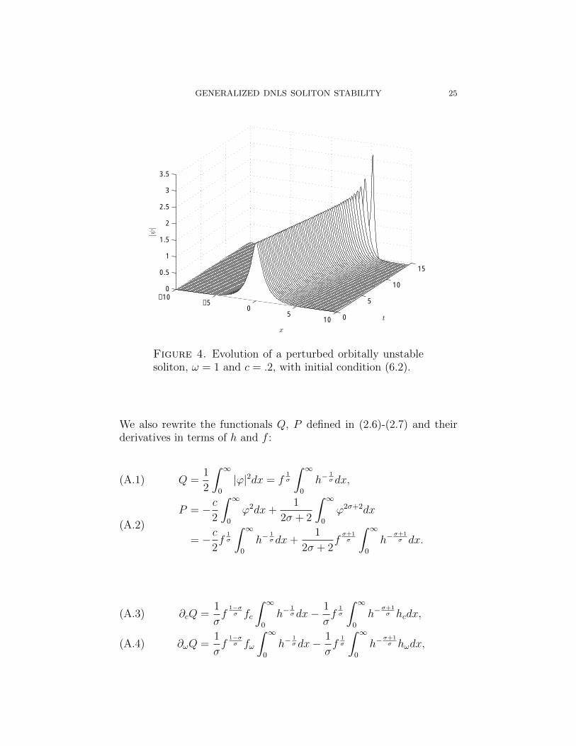
(2) When ω = 1 and c = 0.2 > 2z = 0.1236606, Figure 4 showsthat the amplitude of the solitary wave increases rapidly neart = 10 and it is not orbitally stable.

Our simulation of the unstable soliton suggests that, rather than dis-perse or converge to a stable soliton, gDNLS may result in a finite timesingularity. We will explore the potential for singularity formation inthe forthcoming work [23].

Appendix A. Auxiliary Calculations

In this section, we present certain integral relations that are helpfulin studying the determinant and trace of d′′(ω, c). In the following, wedenote κ =

√4ω − c2 > 0 and rewrite the solitary solution (1.9) as

ϕ(x)2σ = f(ω, c)h(ω, c;x)−1, with

f(ω, c) =(σ + 1)κ2

2√ω

, h(x;σ;ω, c) = cosh(σκx)− c

2√ω.


−10−5

05

10 0

5

10

15

0

0.5

1

1.5

2

2.5

3

3.5

t

x

|ψ|

Figure 4. Evolution of a perturbed orbitally unstablesoliton, ω = 1 and c = .2, with initial condition (6.2).

We also rewrite the functionals Q, P defined in (2.6)-(2.7) and theirderivatives in terms of h and f :

Q =1

2

∫ ∞0

|ϕ|2dx = f1σ

∫ ∞0

h−1σ dx,(A.1)

P = − c2

∫ ∞0

ϕ2dx+1

2σ + 2

∫ ∞0

ϕ2σ+2dx

= − c2f

1σ

∫ ∞0

h−1σ dx+

1

2σ + 2fσ+1σ

∫ ∞0

h−σ+1σ dx.

(A.2)

∂cQ =1

σf

1−σσ fc

∫ ∞0

h−1σ dx− 1

σf

1σ

∫ ∞0

h−σ+1σ hcdx,(A.3)

∂ωQ =1

σf

1−σσ fω

∫ ∞0

h−1σ dx− 1

σf

1σ

∫ ∞0

h−σ+1σ hωdx,(A.4)


∂cP =− 1

2f

1σ

∫ ∞0

h−1σ dx− c

2σf

1−σσ fc

∫ ∞0

h−1σ dx

+c

2σf

1σ

∫ ∞0

h−σ+1σ hcdx+

1

2σf

1σ fc

∫ ∞0

h−1+σσ dx

− 1

2σf

1+σσ

∫ ∞0

h−1+2σσ hcdx

(A.5)

∂ωP =− c

2σf

1−σσ fω

∫ ∞0

h−1σ dx+

c

2σf

1σ

∫ ∞0

h−σ+1σ hωdx

+1

2σf

1σ fω

∫ ∞0

h−1+σσ dx− 1

2σf

1+σσ

∫ ∞0

h−1+2σσ hωdx,

(A.6)

where

fc = −c(1 + σ)√ω

, fω =(1 + σ)(4ω + c2)

4ω3/2,

hc = −σcκx sinh(σκx)− 1

2ω−1/2, hω =

2σ

κx sinh(σκx) +

c

4ω−

32 .

The expressions in (A.3)-(A.6) involve various integrals. The next lem-mas show that all of them can be expressed simply in terms of

αn =

∫ ∞0

h−1σ−ndx.

First, we have

Lemma A.1.

(A.7) α2 =4ω

(σ + 1)κ2α0 +

2c√ω(2 + σ)

(σ + 1)κ2α1

Proof. We first rewrite α0, and then integrate by parts:

α0 =

∫ ∞0

h−1σ−1hdx =

1

σκ

∫ ∞0

h−1σ−1(sinh(σκx))′dx− α1

c

2√ω

=(σ + 1)

σ2

∫ ∞0

h−1σ−2(sinh2(σκx))dx− α1

c

2√ω

=(σ + 1)

σ2

∫ ∞0

h−1σ−2((h+

c

2√ω

)2 − 1)dx− α1c

2√ω.

Regrouping the terms in this last expression, we obtain (A.7). �


Lemma A.2. We have the following relations:∫ ∞0

h−1σ−2hcdx = − 1

2√ωα2 −

cσ

(σ + 1)κ2α1,(A.8) ∫ ∞

0

h−1σ−1hcdx = − 1

2√ωα1 −

cσ

κ2α0,(A.9) ∫ ∞

0

h−1σ−2hωdx =

c

4ω3/2α2 +

2σ

(σ + 1)κ2α1,(A.10) ∫ ∞

0

h−1σ−1hωdx =

c

4ω3/2α1 +

2σ

κ2α0.(A.11)

Proof. By integration by parts, and n integer,∫ ∞0

h−1σ−nhcdx =

c

κ2(− 1σ− n+ 1)

∫ ∞0

h−1σ−n+1dx− 1

2√ω

∫ ∞0

h−1σ−ndx,

Choosing n = 2, 1, we get (A.8) and (A.9). The relations (A.10) and

(A.11) are obtained from (A.8), (A.9) and hω = −2

chc −

κ2

4ω3/2c. �

Using Lemmas A.1 and A.2, we have:

Lemma A.3. Denoting κ = 2−1σ−2σ−1(1+σ)

1σκ2(

1σ−1)ω−

12σ− 1

2 , we have

∂cQ = 2κ[2c(σ − 2)ω1/2α0 + κ2α1

]∂ωQ = κω−1

[(2c2 − 8(σ − 1)ω

)ω1/2α0 − κ2cα1

]∂cP = κ

[(2c2 − 8(σ − 1)ω

)ω1/2α0 − κ2cα1

]∂ωP = 2κ

[2c(σ − 2)ω1/2α0 + κ2α1

].

This is used in Section 4 to obtain (4.1).

References

[1] Agrawal, G.P., Nonlinear Fiber Optics, Academic Press, San Diego, 2006.[2] Colin, M., Ohta, M., Stability of solitary waves for derivative nonlinear

Schrodinger equation, Ann. Inst. H. Poincare, Analyse Non Lineaire, 23 (2006),753–764.

[3] Colliander, J., Keel, M., Staffilani, G., Takaoka, H., Tao, T., A Refined GlobalWell-Posedness Result for Schrodinger Equations with Derivative, SIAM J.Math. Anal., 34 (2002), 64–86.

[4] Comech, A., Cuccagna, S., Pelinovsky, D., Nonlinear instability of a criticaltraveling wave in the generalized Korteweg-de Vries equation, SIAM J. Math.Anal., 39 (2007), 1–33.

[5] Comech, A., Pelinovsky, D., Purely nonlinear instability of standing waves withminimal energy, Commun. Pure Appl. Math., 56 (2003), 1565–1607.


[6] DiFranco, J.C., Miller, P.D., The semiclassical modified nonlinear Schrodingerequation I: Modulation theory and spectral analysis, Physica D, 237 (2008),947–997.

[7] Grillakis, M., Shatah, J., Strauss, W., Stability theory of solitary waves in thepresence of symmetry, I, J. Funct. Anal., 74 (1987), 160–197.

[8] Grillakis, M., Shatah, J., Strauss, W., Stability theory of solitary waves in thepresence of symmetry, II, J. Funct. Anal. 94 (1990), 308–348.

[9] Grunrock, A., Bi-and trilinear Schrodinger estimates in one space dimensionwith applications to cubic NLS and DNLS, Int. Math. Res. Notices, 41 (2005),2525–2558.

[10] Grunrock, A., Herr, S., Low Regularity Local Well-Posedness of the DerivativeNonlinear Schrodinger Equation with Periodic Initial Data, SIAM J. Math.Anal., 39 (2008), 1890–1920.

[11] Guo, B., Wu, Y., Orbital stability of solitary waves for the nonlinear derivativeSchrodinger equation, J. Diff. Eqs., 123 (1995), 35–55.

[12] Hao, C., Well-Posedness for One-Dimensional Derivative NonlinearSchrodinger Equations, Commun. Pure Appl. Anal., 6 (2007), 997–1021.

[13] Hayashi, N., The initial value problem for the derivative nonlinear Schrodingerequation in the energy space. Nonlinear Anal. 20(1993), 823–833.

[14] Hayashi, N., Ozawa, T., On the derivative nonlinear Schrodinger equation.Physica D 55 (1992), 14–36.

[15] Hayashi, N., Ozawa, T., Finite energy solutions of nonlinear Schrodinger equa-tions of derivative type. SIAM J. Math. Anal. 25 (1994), 1488–150.

[16] Hayashi, N. Ozawa, T., Remarks on nonlinear Schrodinger equations in onespace dimension, Diff. Int. Eqs 7 (1994), 453–461.

[17] Kassam, A.K., Trefethen, L.N., Fourth-Order Time-Stepping for Stiff PDEs,SIAM J. Sci. Comput. 26 (2005), 1214-1233.

[18] Kaup, D.J., Newell, A.C., An exact solution for a derivative nonlinearSchrodinger equation, J. Math. Phys., 19 (1978), 798-801.

[19] Kenig, C.E., Ponce, G., Vega, L., Small solutions to nonlinear Schrodingerequations, Ann. Inst. H. Poincare, Analyse Non Lineaire, 10 (1993), 255-288.

[20] Kenig, C.E., Ponce, G., Vega, L., Smoothing effects and local existence theoryfor the generalized nonlinear Schrodinger equations, Invent Math. 134 (1998),489-545.

[21] Lee, J., Global solvability of the derivative nonlinear Schrodinger equation,Trans. Am. Math. Soc. 314 (1989), 107–118.

[22] Linares, F., Ponce, G., Introduction to Nonlinear Dispersive Equations,Springer, Berlin (2009).

[23] Liu, X., Simpson, G., Sulem, C., Numerical simulations of a generelizedDerviative Nonlinear Schroodinger Equation, In preparation.

[24] Marzuola, J.L., Raynor, S., Simpson, G., A system of ODEs for a perturbationof a minimal mass soliton, J. Nonlinear. Sci., 20 (2010), 425-461.

[25] Mio, K., Ogino, T., Minami, K. Takeda, S., Modified Nonlinear SchrodingerEquation for Alfven Waves Propagating along the Magnetic Field in Cold Plas-mas, J. Phys. Soc. 41(1976), 265–271.

[26] Mjølhus, E., On the modulational instability of hydromagnetic waves parallelto the magnetic field, J.Plasma Phys., 16 (1976), 321–334.


[27] Moses, J., Malomed, B., Wise, F., Self-steepening of ultrashort optical pulseswithout self-phase-modulation, Phys. Rev. A, 76 (2007), 1–4.

[28] Ohta, M., Instability of bound states for abstract nonlinear Schrodinger equa-tions, J. Funct. Anal., 261 (2011), 90–110.

[29] Ozawa, T., On the nonlinear Schrodinger equations of derivative type, IndianaUniv. Math. J., 45 (1996), 137–163.

[30] Passot, T., Sulem, P.L., Multidimensional modulation of Alfven waves, Phys.Rev. E, 48 (1993), 2966–2974.

[31] Sulem, C., Sulem, P.L., The nonlinear Schrodinger equation: self-focusing andwave collapse. Applied Mathematical Sciences, vol. 139, Springer, Berlin, 1999.

[32] Tan, S.B., Zhang, L.H., On a weak solution of the mixed nonlinear Schrodingerequations, J. Math. Anal. Appl., 182 (1994), 409–421.

[33] Tsutsumi, M., Fukuda, I., On solutions of the derivative nonlinear Schrodingerequation, Existence and uniqueness theorem, Funkcialaj Ekvacioj, 23 (1980),259–277.

[34] Weinstein, M.I., Modulational Stability of Ground States of NonlinearSchrodinger Equations, SIAM J. Math. Anal., 16 (1985), 472–491.

[35] Weinstein, M.I., Lyapunov Stability of Ground States of Nonlinear DispersiveEvolution Equations, Commun. Pure Appl. Math., XXXIX (1986), 51–68.

Department of Mathematics, University of Toronto

School of Mathematics, University of Minnesota

Department of Mathematics, University of Toronto

stability of solitary waves for a generalized …simpson/files/pubs/lss-stab-final.pdf · stability...

Documents