stability of underground openings in stratified and ... · pdf filestability of underground...
TRANSCRIPT

Stability of underground openings in stratified and jointed rock
Thesis submitted in partial fulfillment of the requirements for the degree of “DOCTOR OF PHILOSOPHY”
by
Michael Tsesarsky
Submitted to the Senate of Ben Gurion University of the Negev
September 05 Kislev, 5765
BEER-SHEVA

This work was carried out under the supervision of
Dr. Yossef Hodara Hatzor
in the Department of Geological and Environmental Sciences
Faculty of Natural Sciences
Abstract I
Stability of underground openings in stratified and
jointed rock
By
Michael Tsesarsky
Department of Geological and Environmental Sciences
Ben Gurion University of the Negev
Abstract
The stability of underground openings excavated in stratified and jointed rock was
studied using the Discontinuous Deformation Analysis method (Shi, 1988; 1993). The goals
of this research were: 1) validation of DDA using analytical solutions, physical models and
case study; 2) investigation of fractured beam kinematics; and 3) development of simplified
design charts for assessment of rock overbrake above excavations as a function of joint
spacing and shear resistance along joints.
Validation of DDA using a shaking table model of a block on an incline (Wartman et
al., 2003) showed that DDA accurately predicts the displacement history of the block,
provided that the numeric control parameters are optimized correctly. It was found that for
slopes subjected to dynamic loading a certain amount of “kinetic” damping is necessary: a 2%
reduction of the inter time-step transferred velocity yielded the best accuracy and the most
realistic time behavior of the modeled system.
Abstract II
Comparison of DDA results with centrifuge model tests a of multi-jointed rock beam
showed that DDA essentially captures the arching stresses developing in a deforming rock
beam. Discrepancies between DDA and measured displacements are attributed to the
difference between the joint model in DDA and the actual block interfaces used in the
centrifuge model.
A study of an ancient roof failure in an underground opening excavated in a densely
jointed rock mass, showed that DDA is more realistic than the classic Voussoir beam model
(Beer and Meek, 1982), which was found to be un-conservative. This research further
augmented the preliminary findings by Hatzor and Benary (1998).
Investigation of fractured beam kinematics shows that transition from shear along
abutments to stable arching is a function of the available shear resistance along joints. Given
sufficient shear resistance the peripheral blocks undergo effective rotation, thus inducing
stable arching. Otherwise, shear along abutments precludes effective rotation, and the beam is
found to sag under its own weight. Within a stack of fractured rock beams the transition from
ongoing deformation to stable arching is marked by the homogenization of the vertical
displacements profile. The transition from unstable conditions to stable arching is found to be
a function of both transverse joint spacing and shear resistance along joints.
The general behavior of underground openings excavated in stratified and vertically
jointed rock masses was studied using two different tunnel geometries: 1) excavation span B
= 10m; and 2) excavation span B = 15m. The modeled tunnel height was ht = 10m for both
configurations. Fifty individual simulations were performed for different values of transverse
joint spacing and shear resistance along joints. It was found that the height of the loosening
zone (or overbrake) above an underground excavation is determined by the ratio between joint
spacing and the excavation span (Sj/B): 1) for Sj/B ≤ 0.2 the height of the loosening zone is

Abstract III
found to be smaller than 0.5B; 2) for Sj/B ≥ 0.3 the rock mass above the excavation attains
stable arching.
Terzaghi’s (1946) rock load classification for a blocky rock mass predicts that the rock
load above the excavation should range from 0.25B to 1.1(B+ht), pending on the degree of
jointing. However, the degree of jointing is not quantified, and guidelines for assessing the
degree of jointing are not provided. When compared with the findings of this research
Terzaghi’s predictions are found to be rather conservative.
The contribution of this study lies in the explicit correlation between the geometrical
features of the rock mass, which are routinely collected during exploration and excavation,
and the extent of the instability zone above the excavation. This is expected to contribute to a
more efficient and economic design, and to increase the safety of underground openings in
stratified and jointed rocks.

This Work is Dedicated to My Beloved Wife Galia
Table of Contents i
Table of Contents
Table of Contents .................................................................................................................... i
List of Figures.......................................................................................................................... iv
List of Tables ........................................................................................................................... viii
Acknowledgments ................................................................................................................... ix
Nomenclature .......................................................................................................................... xi
Chapter 1 - Introduction 1
1.1 Overview ........................................................................................................................... 1
1.2.Objectives .......................................................................................................................... 2
1.3. Thesis Organization.......................................................................................................... 2
Chapter 2 - Stability Analysis of Underground Openings in a Stratified and Jointed Rock Mass 4
2.1. Introduction ...................................................................................................................... 4
2.2. Observational Methods..................................................................................................... 6
2.3. Semi-analytical Approach – the Voussoir Beam Analogy............................................... 10
2.4. Numerical Approach ........................................................................................................ 13
2.4.1. The Finite Element Method....................................................................................... 13
2.4.2. The Discrete Element Method (DEM) ...................................................................... 14
2.5. Numerical Modeling of the Voussoir Beam Using FEM and DEM ................................ 15
2.6. Physical Modeling of the Voussoir Beam ........................................................................ 16
2.7. Case Studies...................................................................................................................... 18
2.8. Current Research Motivation ........................................................................................... 19
Chapter 3 – DDA Basics: Review of Fundamentals 20
3.1. Formulation of Simultaneous Equilibrium Equations ..................................................... 20
3.2. Energy Functionals and Contributions to Global Equilibrium Equations ....................... 23
3.3. Block System Kinematics and Contacts .......................................................................... 27
3.3.1. Distance between two blocks .................................................................................... 28
3.3.2. Contacts and interpenetration .................................................................................. 29
3.3.3. Energy functional of a stiff contact........................................................................... 30

Table of Contents ii
3.3.4. Limitations of DDA stiff contact formulation ........................................................... 33
3.4. Time Integration Scheme................................................................................................. 34
3.5. DDA Numeric Implementation........................................................................................ 37
Chapter 4 – Validation of DDA Using Analytical Solutions and Shaking Table Experiments 40
4.1. Introduction...................................................................................................................... 40
4.2. Validation of DDA Using an Analytical Solution ........................................................... 41
4.3. Validation of DDA by Shaking Table Experiments ........................................................ 47
4.3.1 Experimental setting .................................................................................................. 47
4.4. DDA Prediction vs. Shaking Table Results ..................................................................... 53
4.4.1. Accuracy of DDA........................................................................................................... 54
4.5. Conclusions...................................................................................................................... 59
Chapter 5 – Validation of DDA Using a Centrifuge Model of a Jointed Rock Beam 60
5.1. Introduction...................................................................................................................... 60
5.2. Experimental Setting........................................................................................................ 61
5.2.1.Jointed beam model ................................................................................................... 61
5.3. DDA Model ................................................................................................................. 62
5.3.1 A simple two-block system ......................................................................................... 62
5.3.2. A six block model ...................................................................................................... 66
5.3.3. Selection of numerical control parameters............................................................... 66
5.3.4. Results....................................................................................................................... 72
5.4. Discussion and Conclusions ............................................................................................ 76
Chapter 6 – The Tel Beer-Sheva Case Study 76
6.1. Introduction...................................................................................................................... 76
6.2. Site Description................................................................................................................ 77
6.2.1. Geology..................................................................................................................... 78
6.2.2. Geometrical properties of discontinuities and failure zone morphology ................. 78
6.3. Mechanical Properties of Intact Rock.............................................................................. 81
6.3.1. Experimental procedure ........................................................................................... 81
6.3.2. Test results ................................................................................................................ 84
6.3.3. Estimation of the in-situ stresses .............................................................................. 84
6.4. Mechanical Properties of Discontinuities ........................................................................ 88

Table of Contents iii
6.4.1. Direct Shear testing apparatus and sample preparation.......................................... 88
6.4.2. Direct shear tests of natural joint ............................................................................. 89
6.4.3. Shear rate effect – polished interface ....................................................................... 89
6.4.4. Direct shear tests of a polished interface ................................................................. 90
6.5. Stability Analysis Using Classical Voussoir Model ........................................................ 97
6.6. Numerical Analysis Using DDA ..................................................................................... 101
6.6.1. Numerical problems associated with multi-block systems ....................................... 101
6.6.2. DDA analysis of the Tel Beer-Sheva water reservoir – numerical setup ................. 104
6.6.3. DDA analysis of the single layer configuration........................................................ 107
6.6.4. DDA analysis of sequence of layers - laminated Voussoir beam ............................. 112
6.6.5. Limitations of DDA................................................................................................... 113
6.6.6. Comparison between DDA and classic Voussoir solutions...................................... 119
Chapter 7 - Stability Analysis of Underground Openings in Horizontally Stratified and Vertically Jointed Rock 120
7.1. Introduction...................................................................................................................... 120
7.1.1. Model geometry and mechanical properties ............................................................ 121
7.1.2. Selection of contact stiffness ..................................................................................... 125
7.1.3. Criteria for stable arching........................................................................................ 127
7.2. Results.............................................................................................................................. 128
7.2.1. Roof span of 10m ...................................................................................................... 128
7.2.2. Influence of joint randomness................................................................................... 130
7.2.3. Roof span of 15m ...................................................................................................... 137
7.2.4. Rock mass response as a function of excavation span.............................................. 142
7.3. Discussion ........................................................................................................................ 146
Chapter 8 – Conclusions 151
8.1. DDA Limitations ............................................................................................................. 152
8.2. DDA Accuracy................................................................................................................. 153
8.3. DDA Validation ............................................................................................................... 153
8.4. Stability of Underground Openings in Horizontally Stratified and Vertically Jointed Rock ................................................................................................................................. 156
8.5. Recommendations for Future Research ........................................................................... 158
Appendix 160
References 164

List of Figures iv
List of Figures Figure 2.1. a) Horizontally laminated rock mass and immediate roof deflection; b)
Horizontally laminated rock mass with vertical joints (after Brown and Brady, 1993) ................................................................................................................................... 5
Figure 2.2. Maximum expected over-brake for unsupported tunnels: a) horizontally stratified rock (top); b) vertically stratified rock (bottom). From Terzaghi (1946). ........... 8
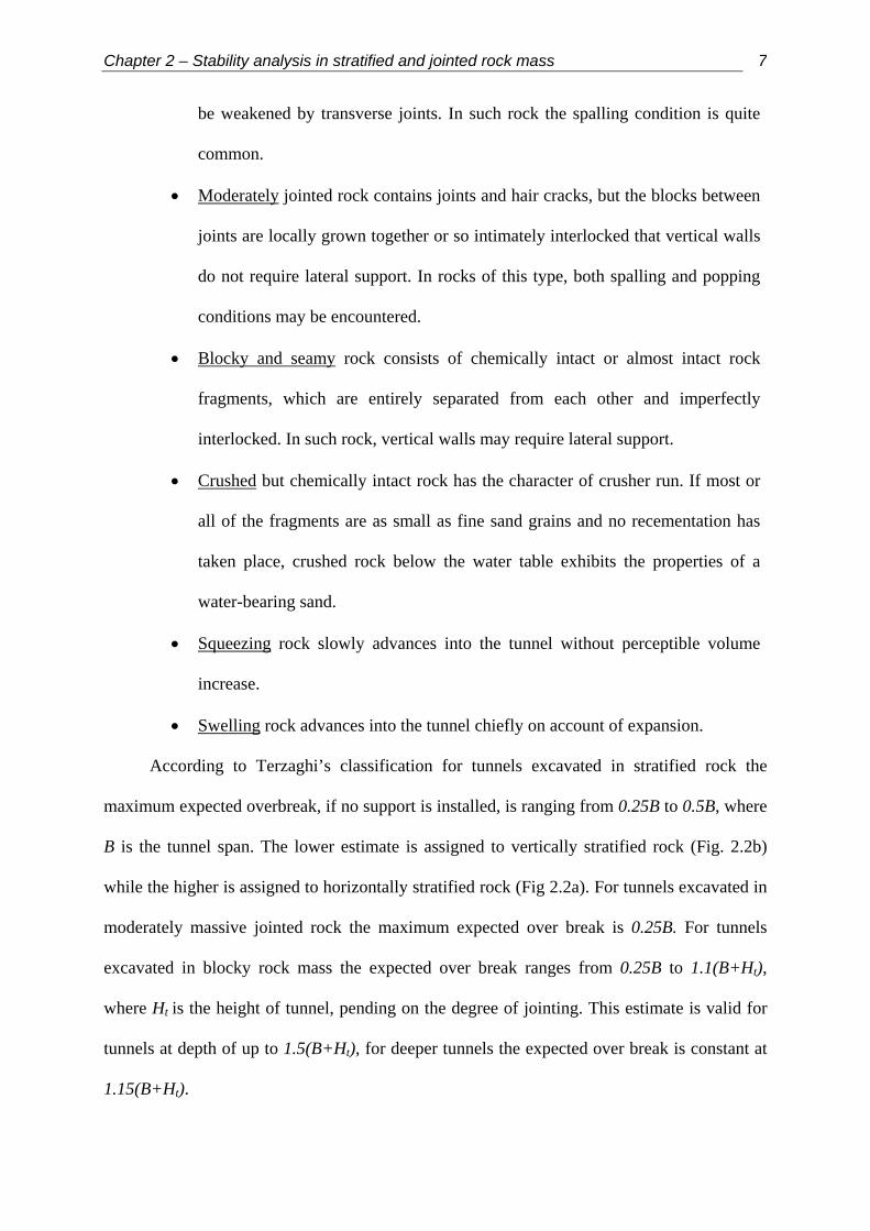
Figure 2.3. Evans’s Voussoir beam: a) conceptual model; b) compressive stress distribution in the beam. ..................................................................................................... 12
Figure 3.1. Distance of two blocks (after Shi, 1993) ................................................................... 28
Figure 3.2.Types of blocks contact: a) angle to edge; b) angle to angle; c) edge to edge (after Shi,1993). .................................................................................................................. 29
Figure 3.3 Contact conditions: a) overlapping angle and edge; b) overlapping angles (modified after Shi,1993).................................................................................................... 30
Figure 3.4. A wedge loaded by normal and tangential forces at the apex (after Timoshenko and Goodier, 1951) ........................................................................................ 33
Figure 3.5. Two block system. ..................................................................................................... 36
Figure 3.6. DDA results for the two block system: for a time step size of g1 = 0.005 sec a) vertical stress at the centroid of the upper block for different values of contact stiffness; b) relative numeric error for different values of contact stiffness. ...................... 38
Figure 3.7. DDA results for the two block system for contact stiffness of g0 = 50•106 N/m: a) vertical stress at the centroid of the upper block for different values of time step size (g1) ; b) relative numeric error for different values of time step size (g1)...................................................................................................................................... 39
Figure 4.1. a) the loading function a(t) = a1sin(ωt) + a2sin(ω2t)+ a3sin(ω3t); b) comparison between analytical and DDA solution for block displacement subjected to a loading function consisting of a sum of three sines..................................... 44
Figure 4.2. Sensitivity analysis of the DDA numeric control parameters. 45 Figure 4.3. Sinusoidal input motion for the shaking table experiment: 2.66 Hz frequency
(Test 1 at Table 4.2). .......................................................................................................... 49
Figure 4.4. a) general view of the inclined plane and the sliding block (top); b) sliding block experimental setup and instrumentation location (bottom), from Wartman (1999). ................................................................................................................................ 50
Figure 4.5. Back analyzed friction angles shown as a function of average sliding velocity for rigid block tests, from Wartman (2003). ........................................................ 51
Figure 4.6. The 2.66 Hz sinusoidal input motion test: a) displacement derived velocity; b) velocity content. ............................................................................................................ 52
List of Figures v
Figure 4.7. The 2.66 Hz input motion: comparison between measured displacement and DDA solutions for different values of inter time step velocity reduction (k01). ............... 57
Figure 4.8. The 2.66 Hz input motion: relative numeric error of DDA ultimate displacement as a function of inter time step velocity reduction (k01). ............................ 57
Figure 4.9. Numeric difference of DDA ultimate displacement prediction as a function of input motion frequency. ................................................................................................. 58
Figure 4.10. The 2.66 Hz input motion: evolution over time of the DDA relative numeric error, for different values of the k01 parameter. .................................................. 58
Figure 5.1 Centrifuge model geometry and instrumentation (courtesy of M. Talesnick)............ 63
Figure 5.2 DDA model geometry. ............................................................................................... 63
Figure 5.3. DDA model of two block system with fixed base vertices: a) mid-span deflection (�) as a function of time; b) number of time steps n required to attain equilibrium as a function of the dynamic control parameter (k01). ................................... 64
Figure 5.4. Contact stiffness sensitivity analysis for the DDA six block model: a) vertical displacements; b) horizontal stresses within the blocks. ....................................... 69
Figure 5.4 b) Contact stiffness sensitivity analysis for the DDA six block model: c) time histories. ............................................................................................................................. 70
Figure 5.5. Iteration history for the DDA six block model for different values of contact stiffness. ............................................................................................................................. 71
Figure 5.6. DDA six block model loading function. ................................................................... 73
Figure 5.7. Comparison between centrifuge model results and DDA solution: a) vertical displacements; b) horizontal stresses. ................................................................................ 74
Figure 5.8. DDA six block model: angle to principal stresses (θ) within the blocks .................. 75
Figure 6.1. Schematic drawing of the Tel Beer-Sheva archeological site and the water reservoir. (Source: Hatzor and Benari, 1998). ................................................................... 79
Figure 6.2 General layout and failure zone mapping of the water reservoir, after Benary (1996).................................................................................................................................. 82
Figure 6.3. Cross-sections of the water reservoir......................................................................... 83
Figure 6.4 Complete stress-strain curves for the Gareb chalk at uniaxial compression parallel and normal to bedding .......................................................................................... 86
Figure 6.5. a) Calculated and measured stress ratio k at the Beer-Sheva syncline; b) horizontal and vertical stresses at the Beer-Sheva syncline. .............................................. 87
Figure 6.6. Direct shear system at the Rock Mechanics Laboratory of the Negev: a) general view; b) assembled shear box and displacement detectors (LVDT’s)................... 92

List of Figures vi
Figure 6.7. Direct shear results of a natural joint in Gareb formation, sample TBS-1. ............... 93
Figure 6.8. Direct shear results for polished surface in Gareb chalk, sample TBS – 2................ 94
Figure 6.9. Direct shear results for a polished surface, sample TBS-4. ....................................... 95
Figure 6.10. Sample TBS-4: normal displacement vs. shear displacement at different levels of normal stress......................................................................................................... 96
Figure 6.11. Classic Voussoir beam analysis of the Tel Beer-Sheva water reservoir.................. 99
Figure 6.13. DDA multi block model: average number of iterations per time step as a function of penalty stiffness (g0) for different values of time step size (g1) and penetration control parameter (g2). .................................................................................... 103
Figure 6.14. Geometry of DDA model of the Tel Beer-Sheva water reservoir: a) single layer model; b) multi-layered model. ................................................................................. 106
Figure 6.15. DDA prediction for mid-span deflection of the single layer model...................... 109
Figure 6.16. Deformation profiles of the DDA single layer model, measured at the lowermost fiber of the beam/ ........................................................................................... 110
Figure 6.17. DDA graphic output of single layer deformation for different values of joint friction angle............................................................................................................... . 111
Figure 6.18. a) DDA prediction for mid-span deflection of the multi-layered model. ................ 116
Figure 6.19. DDA graphic output of the multi-layer deformation for different values of joint friction angle............................................................................................................... 117
Figure 7.1.Geometry of the DDA model...................................................................................... 124
Figure 7.2. Two types of rock masses. ......................................................................................... 124
Figure 7.3. Contact stiffness sensitivity analysis for a DDA model of tunnel span B = 10m and vertical joints spacing Sj = 1.5............................................................................. 126
Figure 7.4. DDA graphic output for tunnel span of B = 10m and vertical joint spacing of Sj = 1.5: a) initial configuration (top); b) deformed configuration (bottom). 131
Figure 7.5.Vertical displacement (δ) profile above an underground opening of span B = 10m, for different values of joint spacing (Sj) and friction along joints (φ). ...................... 132
Figure 7.6. Vertical displacement difference (∆δ/∆y) profile above an underground opening of span B = 10m, for different values of joint spacing (Sj) and friction along joints (φ). .................................................................................................................. 133
Figure 7.7. Rock mass response above an underground opening of span B = 10m, and joint spacing of Sj = 1.5m................................................................................................... 135
Figure 7.8. DDA graphic output for tunnel span of B = 10m, vertical joint spacing of Sj

List of Figures vii
= 1.5m with random ........................................................................................................... 136
Figure 7.9. Vertical displacement (δ) profile above an underground opening of span B = 15m, for different values of joint spacing (Sj) and friction along joints (φ). ...................... 138
Figure 7.10. Vertical displacement difference (∆δ/∆y) profile above an underground opening of span B = 15m, for different values of joint spacing (Sj) and friction along joints (φ). ................................................................................................................... 139
Figure 7.11. DDA graphic output for tunnel of span B = 15m, vertical joint spacing of Sj = 2m and friction angle of φ = 20o...................................................................................... 140
Figure 7.12. DDA graphic output for tunnel of span B = 10m, vertical joint spacing Sj = 2 and friction angle of φ = 20o m. ...................................................................................... 141
Figure 7.13. Normalized displacement δ/B for normalized joint spacing of Sj /B = 0.2. ............ 143
Figure 7.14. Vertical displacement ratio δB=15/δB=10 for different values of normalized joint spacing Sj /B. .......................................................................................... 144

List of Tables viii
List of Tables Table 4.1. Frequency sets for a loading function consisting of a sum of three sines................... 43
Table 4.2. Shaking table model summary. ................................................................................... 49
Table 5.1. Material properties and numeric control parameters for the DDA six block model. ................................................................................................................................. 73
Table 6.1. Principal joint sets in the Gareb chalk at Tel Beer-Sheva site, from Benary (1996).................................................................................................................................. 79
Table 6.2. Mechanical properties of the Gareb chalk at Tel Beer-Sheva..................................... 86
Table 6.3. Shear stiffness at different shear rate values for sample TBS – 2............................... 94
Table 6.4. Representetive material l properties of the Gareb Chalk. ........................................... 97
Table 6.5. Material properties and numeric control parameters for the DDA model of the Tel Beer-Sheva water reservoir. .................................................................................. 105
Table 7.1. DDA modeling matrix................................................................................................. 122
Table 7.2 Locations of measurement points in DDA model. X,Y coordinates are with respect to the center of the geometrical domain. ............................................................... 123
Table 7.3. Material properties and numeric control parameters for DDA model. . ..................... 123
Table 7.4. Normalized height of loosening zone (hr = h/ht) above an underground opening for a horseshoe tunnel of width B = 10m and height ht = 10m............................. 130
Table 7.5. Normalized height of loosening zone (hr = h/ht) above an underground opening, for a horseshoe tunnel of width B = 15m and height ht = 10m............................ 145
Table 7.6. Normalized height of the loosening zone (hr = h/ht) above an underground opening for different values of joint spacing and opening span (Sj/B). .............................. 147

Acknowledgments ix
Acknowledgments
I was privileged to conduct this research under the guidance of Dr. Yossef Hodara
Hatzor. His wisdom and philosophy greatly enhanced my professional and personal
development. For all that and much more I am greatly indebted.
I would like to thank Dr. Gen-hua Shi the father of DDA, and many other wonderful
ideas, for the privilege to work with DDA. His short visits to Israel were always enlightening
and instructive.
Dr. Mark Talesnick from the Technion has devised and executed the centrifuge tests of
the fractured rock beams. His engineering ingenuity, experimental creativity, and cooperation
are greatly acknowledged.
I thank Prof. Nicholas Sitar from the University of California, Berkeley for his
assistance during the initial stages of this research. Professor Joseph Wartman of Drexel
University, and Professors Jonathan Bray and Raymond Seed from University of California,
Berkeley are thanked for providing the test data for the shaking table model. Dr. David
Doolin is thanked for his valuable suggestions and productive dialog on DDA essentials.
Dr. V. Palchick from the Rock Mechanics Laboratory of the Negev, BGU is thanked for
his assistance with rock testing.
This work was partially supported by the Israel-USA Bi-National Science Foundation
(BSF) through grant number 98-339. The BSF support is kindly acknowledged.
I would like to thank Prof. Yehuda Eyal from the Department of Geological and
Environmental Sciences, BGU for his support and encouragement during all my years as
graduate student.
Prof. S. Freedman from the Faculty of Civil Engineering, Technion and Prof. M. Perl
from the Department of Mechanical Engineering, BGU served on my Ph.D. candidacy

Acknowledgments x
committee. They are thanked for putting me on the right track. It wasn’t easy, but definitely
worthy.
It has been a great pleasure to study and work in the Department of Geological and
Environmental Sciences, BGU. I have learned much from the faculty of the Department of
Geological and Environmental Sciences and would like to thank in particular Prof. M. Eyal
and Prof. H. J. Kisch.
I thank the administrative staff of our department, firmly headed by Mrs. Rivka Eini.
She was always there to smoothen up bureaucracy, and to help with everything within (and
beyond) her mandate. The technical staff of the department is thanked for all the support
provided during the years. Special thanks are extended to Mr. D. Kozashvily.
I would like to thank my fellow graduate students for the years we spent together.
Special thanks are extended to Shai Arnon, Shai Ezra, Sigal Abramovich, Efi Farber, Anat
Bernstein, Zafrir Levy, Ilanit Tapiero, and Boaz Saltzman.
My friends: Erez and Galit Tzfadia, Sagee and Dorit Levy, Sami and Orly Ohana, Shai
and Iris Ezra, Tal and Simon Tamir, who were there to support and encourage, your
friendship is beyond words.
I would like to express my deepest gratitude to my parents who planted the seed of
curiosity and inquisitiveness. I am also grateful to all other members of my family: my elder
brother Ilia his wife and children.
Last but dearest my wife Galia. The last five years were hard. I could not make it trough
without your love, friendship, care, endurance and patience. This work is dedicated to you.

Nomenclature xi
Nomenclature
Symbol Description Chapter
W weight of Voussoir beam Apendix S span of Voussoir beam T axial thrust Z lever arm of the axial couple t Voussoir beam thickness n thickness of compressive arch γ unit weight fc maximum compressive stress L length of the reaction arch fav average stress along the compression arch UCS uniaxial compressive strength φ friction angle (u, v) displacement of a point 3.1 (x, y) coordinates of a point εx x-direction strain εy y-direction strain γxy shear strain (x0, y0) center of gravity (u0, v0) block translation (r0) block rotation angle [Di] unknowns of block i [Ti] displacement matrix of block i Kij submatrix of equilibrium equations [K] global stiffness matrix Fi loads on block i {F} load vector Π total potential energy Πe strain energy of block σx x-direction stress 3.2 σy y-direction stress τxy shear stress E Elasticity modulus S area of block i Πp potential energy of point load fx, fy x, y directions of point load Πl potential energy of line load

Nomenclature xii
Symbol Description Chapter
Fx(t), Fy(t) parametric equations for x, y directions of line load l length of segment Πw potential energy of volume load Πi potential energy of inertia force M mass per unit area ηij distance between two blocks 3.3 Πc potential energy constraint spring p stiffness of constraint spring u displacement of a point 3.4 u velocity of a point u acceleration of a point ∆t integration time step β, γ integration collocation parameters en relative numeric error a acceleration 4 ω frequency g Earth gravitational accelaration ρ material density 5 h depth N scaling factor i total number of iterations 6 iav average number of iteration per time step k horizontal to vertical stress ratio δ mid span deflection Sj average joint spacing Lj average joint length 7 Bj average joint bridge Dr degree of randomness B tunnel span ht tunnel height hr loosening zone height
Chapter 1 - Introduction 1
Chapter 1 - Introduction
1.1. Overview
Most rock masses are discontinuous over a wide range of scales, from macroscopic to
microscopic. In sedimentary rocks the two major sources of discontinuities are: 1) bedding
planes, and 2) joints. Bedding planes are formed due to sedimentary processes, while joints
are formed by lithification processes or by tectonic forces. The intersection of bedding planes
and joints forms the so-called “blocky” rock mass.
Before the excavation of an underground opening the blocky rock mass is assumed to
be in a state of static equilibrium and in optimum packing arrangement. Excavation of an
opening disturbs the initial equilibrium, and the stresses in the rock mass tend to readjust until
new equilibrium is attained. During the readjustment of the internal stresses, and hence the
rearrangement of load resisting forces, some displacements of the rock blocks occurs. Failure
occurs when the stresses can no longer readjust to form a stable, load resisting structure. This
may occur either when the material strength is exceeded at some locations or when
movements of the rock blocks preclude stable geometric configuration, without strength
failure.
Joints and beddings are sources of weakness in an otherwise competent rock mass,
therefore large displacements and rotations are only possible across these discontinuities. The
displacements and rotations of the rock block along and across the joints is the source of the
volume change. The interaction forces between blocks result in: 1) an increase in formation

Chapter 1 - Introduction 2
stresses, due to volume expansion in restricted volume, tending to create stable conditions;
and 2) application of forces that can cause an increased displacement, tending to induce rock
mass failure. The interaction between the stabilizing and destabilizing factors shape the
overall behavior of the blocky rock mass.
1.2. Objectives
The research presented in this dissertation focuses on the kinematical behavior of
underground openings in layered and jointed rock masses. The primary objectives of this
research are: 1) validation of the numeric Discontinuous Deformation Analysis (DDA) model
using physical models and case studies; 2) investigation of fractured beam kinematics; 3)
development of simplified design charts and tables for assessment of rock loads in
underground openings as a function of joint spacing and joint friction angle.
1.3. Thesis Organization
Chapter 2 is a brief overview of the techniques commonly used in engineering practice
for estimating the stability of underground openings in blocky rock masses. The different
approaches are described and discussed, and the limitations are addressed.
Chapters 3 describes the theoretical background of the Discontinuous Deformation
Analysis (DDA) method and previous validation effort. Following is the validation of DDA
using a shaking table physical model (Wartman et al, 2003) presented in Chapter 4. The
results of the validation study are discussed and recommendations of numeric improvements
are presented. Chapter 5 describes DDA validation using centrifuge model testsof a jointed
beam, which were performed by M. Talesnick at the Technion.

Chapter 1 - Introduction 3
Chapter 6 describes DDA validation using the case study of the ancient water reservoir
at the Tel Beer-Sheva archeological site, which was studied initially by Hatzor and Benary
(1998). The system was excavated in highly layered and jointed rock mass. The re-visited
case study is here described in detail, including physical testing of intact rock and the
discontinuities. The results are discussed, and general conclusions regarding behavior of
blocky rock masses are presented.
Chapter 7 presents an investigation of the general behavior of layered and jointed roofs.
Simplified design charts based on geometrical properties of the discontinuities are presented
and discussed. Finally, Chapter 8 summarizes the key findings of this research and makes
suggestions regarding future research.

Chapter 2 – Stability analysis in stratified and jointed rock mass 4
Chapter 2 - Stability Analysis of Underground Openings in
a Stratified and Jointed Rock Mass
2.1. Introduction
A stratified host rock mass is a common feature in mining and civil engineering where
excavation in sedimentary rock is attempted. Stratified rock (Fig. 2.1a) is defined as
composed of a succession of parallel layers whose thickness is small compared with the span
of the opening (Obert and Duvall, 1976). There are two principal mechanical properties of
bedding planes that are significant in the context of underground projects : 1) low to zero
tensile strength; 2) low shear strength. If an opening is excavated in this type of rock the roof
of the excavation will part from the rock mass due to low tensile strength of bedding planes,
thus forming the immediate roof. Investigation of immediate roof stability commenced more
than a century ago when Fayol (1885) conducted experiments on a stack of wood beams
spanning a simple support, simulating the bedded sequence of roof span. By noting the
deflection of the lowest beam as successive beams where loaded onto the stack, Fayol
demonstrated that at a certain stage none of the added load of an upper beam was carried by
the lowest member. The load of the upper beams was transmitted laterally to the supports,
rather than vertically as transverse loads to the lower members. For such a configuration beam
theory can be employed to assess deflection, shear stresses, and maximum stresses in the
immediate roof as a function of elastic parameters, rock density, and beam geometry (Obert

Chapter 2 – Stability analysis in stratified and jointed rock mass 5
and Duvall, 1976). Goodman (1989) incorporated inter-bedding friction into the beam
analysis, thus extending the capabilities of this method. These analyses however are limited to
continuous, clamped beams only.
Immediate roofdeflection
Bedding planesa
Immediate roofdeflection
Bedding planesa
Bedding planes Jointsb
Bedding planes Jointsb
Figure 2.1. a) Horizontally laminated rock mass and immediate roof deflection; b) Horizontally laminated rock mass with vertical joints (after Brown and Brady, 1993)
Chapter 2 – Stability analysis in stratified and jointed rock mass 6
In practice, stratified rock masses are in most cases transected by numerous joints
forming a matrix of individual rock blocks. Horizontal stratification with vertical jointing one
common case (Fig. 2.1b). The analysis of a stratified and jointed roof is complicated by the
fact that there is no closed-form analytical solution for the interaction of these blocks. In
absence of a closed-form solution, the practicing engineer/geologist should rely on other
methods for assessing the stability of the roof. Three different methods are currently in
practice: 1) observational methods; 2) semi-analytical methods; 3) numerical methods. These
methods are widely used today, either stand alone or in an integrated manner, in all areas of
geological and civil engineering.
2.2. Observational Methods
Standard engineering design both in continuous and structurally discontinuous rock is
largely based on observational methods known as rock mass classification methods, mostly
assessing the expected stand-up time and the required support loads.
Terzaghi (1946) formulated the first rational method of classification by evaluating the
rock loads appropriate to the design of steel sets, based on rock mass description. Terzaghi’s
descriptions are:
• Intact rock contains neither joints nor hair cracks. Hence, if it breaks, it breaks
across sound rock. On account of the injury to the rock due to blasting, spalls
may drop off the roof several hours or days after blasting. Hard, intact rock
may also be encountered in the popping condition involving the spontaneous
and violent detachment of rock slabs from the sides or roof.
• Stratified rock consists of individual strata with little or no resistance against
separation along the boundaries between the strata. The strata may or may not
Chapter 2 – Stability analysis in stratified and jointed rock mass 7
be weakened by transverse joints. In such rock the spalling condition is quite
common.
• Moderately jointed rock contains joints and hair cracks, but the blocks between
joints are locally grown together or so intimately interlocked that vertical walls
do not require lateral support. In rocks of this type, both spalling and popping
conditions may be encountered.
• Blocky and seamy rock consists of chemically intact or almost intact rock
fragments, which are entirely separated from each other and imperfectly
interlocked. In such rock, vertical walls may require lateral support.
• Crushed but chemically intact rock has the character of crusher run. If most or
all of the fragments are as small as fine sand grains and no recementation has
taken place, crushed rock below the water table exhibits the properties of a
water-bearing sand.
• Squeezing rock slowly advances into the tunnel without perceptible volume
increase.
• Swelling rock advances into the tunnel chiefly on account of expansion.
According to Terzaghi’s classification for tunnels excavated in stratified rock the
maximum expected overbreak, if no support is installed, is ranging from 0.25B to 0.5B, where
B is the tunnel span. The lower estimate is assigned to vertically stratified rock (Fig. 2.2b)
while the higher is assigned to horizontally stratified rock (Fig 2.2a). For tunnels excavated in
moderately massive jointed rock the maximum expected over break is 0.25B. For tunnels
excavated in blocky rock mass the expected over break ranges from 0.25B to 1.1(B+Ht),
where Ht is the height of tunnel, pending on the degree of jointing. This estimate is valid for
tunnels at depth of up to 1.5(B+Ht), for deeper tunnels the expected over break is constant at
1.15(B+Ht).

Chapter 2 – Stability analysis in stratified and jointed rock mass 8
Figure 2.2. Maximum expected overbrake for unsupported tunnels: a) horizontally stratified rock (top); b) vertically stratified rock (bottom). From Terzaghi (1946).

Chapter 2 – Stability analysis in stratified and jointed rock mass 9
The definitions of the different rock classes in Terzaghi’s method are ambiguous, and
no particular reference to the mechanical and geometrical properties of the discontinuities is
given.
Lauffer (1958) introduced the concept of Stand-Up Time, which estimates the time to
failure for any active unsupported span as a function of rock structure. Lauffer’s original
classification has since been modified by a number of authors, notably Pacher et al (1974),
and now forms part of the general tunneling approach known as the New Austrian Tunneling
Method (NATM).
Development of new support techniques, i.e. the use of rock bolts and shotcrete, gave
rise to new Rock Mass Classification Methods encompassing all aspects of support design:
from stand-up time to support requirements. Two of the most prominent methods are the
Geomechanics Classification (a.k.a. Rock Mass Rating -RMR) of Bieniawski (1973) and the
Rock Quality system of Barton et al., (1974) both based on extensive database of case studies.
In each method the critical parameters of the rock mass are described and rated, and simple
equations yield the overall rock mass rating. Based on the rock mass rating a support design is
suggested, as well as the unsupported stand-up time. These observational methods are widely
used today by practitioners world wide, mostly as checkup on their design.
Two major drawbacks of the rock mass classification methods are to be noted: 1) rock
mass classifications are a very general and a rather coarse approach in that it caters for all
possible rock masses and type of excavation; 2) absence of mechanistic basis. Recent studies
in Israel (Polishook and Flexer, 1998; Tsesarsky and Hatzor, 2000) show that these methods
are in some cases over conservative, even when a simple rock mass is encountered
(homogenous massive rock with widely spaced joints). Riedmuller and Schubert (1999),
based on extensive tunneling practice in the Austrian Alps, show that rock mass classification
is inadequate for support design and stability evaluation in complex geological conditions.

Chapter 2 – Stability analysis in stratified and jointed rock mass 10
The absence of true understanding of deformation mechanisms and the over conservative
nature of the empirical methods will eventually lead to over conservative support design and
unnecessary inflated project costs (Riedmuller and Schubert, 1999).
2.3. Semi-analytical Approach – the Voussoir Beam Analogy
As noted by Fayol (1885) underground strata tend to separate upon deflection such that
each laminated beam transfers its own weight to the abutments rather than loading the beam
beneath. Stability of the excavation in this situation can be determined by analyzing the
stability of a single beam deflecting under its own weight. Bucky (1931) and Bucky and
Taborelli (1938) studied physical models for the creation and extension of wide roof spans.
They used initially intact beams of rock like materials, and found that at a particular span, a
vertical tension fracture was induced at the mid-span of the lower beam. These observations,
and the fact that roof strata are crossed by joints, lead to the conclusion that the roof at
incipient failure cannot be treated as a simple beam.
Evans (1941) in his fundamental work established the relationship between vertical
deflection, lateral thrust and stability of natural or artificially jointed roof. This work coined
the term “Voussoir Beam” spanning an excavation, using the analogy of the masonry
Voussoir arch (Heyman, 1982). The basic Voussoir concept accepts that the beam may not
carry longitudinal tensile stresses and it is confined between the abutments, i.e. lateral
constrains are applied. The geometry and the forces acting in the Voussoir beam are shown in
Figure 2.3a. The overturning gravitational-reaction couple is equilibrated by the lateral thrust
couple formed by beam deflection, where W is the weight of the beam, S is the beam span, T
is the axial thrust and Z is the lever arm.
The structure presented in Figure 2.3a is statically indeterminate since the lever arm Z is
not known. In order to treat the posed problem analytically Evans assumed that a parabolic

Chapter 2 – Stability analysis in stratified and jointed rock mass 11
compressive arch structure of constant thickness is formed within the beam (Fig 2.3b). He
also assumed an identical thickness of the arch at the abutments and at mid-span equal to half
of the beam thickness. Three modes of failure are considered: 1) crushing of the rock at the
abutments or at mid-span; 2) buckling (snap through) failure of the beam; 3) sliding between
the blocks and the abutments.
Beer and Meek (1982) reformulated and extended Evans’s approach, introduced a
coherent system of static equations, and evaluated the thickness of the compressive arch at the
abutments and mid-span. Brady and Brown (1985) summarized the above-mentioned work
and introduced an iterative algorithm for the evaluation of Voussoir beam stability. The
iterative approach assumes initial load distribution and line of action, i.e. assuming initial n
and Z. The analysis provides the compressive zone thickness, and the maximum axial thrust.
The factor of safety against the previously mentioned failure modes can be calculated
provided that the compressive strength of the rock, and the shear strength of the
discontinuities are known. Sofianos (1996) statistically evaluated compressive arch thickness
values, from the numerical data for different beam geometries provided by Wright (1974),
thus eliminating static indeterminacy. Diederichs and Kaiser (1999) further improved the
classic iterative approach by introducing improved assumptions for lateral stress distribution
and arch compression, and by providing a numerical buckling limit.
The major advantages of the Voussoir beam technique are the ability to assess
previously ignored failure by shear along the abutments, and providing static (although
undetermined) formulation of the discussed problem. Two main disadvantages of this method
regarding the actual geometry of the problem should be mentioned.
Chapter 2 – Stability analysis in stratified and jointed rock mass 12
S
t
tnt
S4
W2
Z
fc
V
T
Mid-Span Crack
Voussoirblock Abutment
a
b
Figure 2.3. Evans’ Voussoir beam: a) conceptual model; b) compressive stress distribution in the beam.

Chapter 2 – Stability analysis in stratified and jointed rock mass 13
First, the Voussoir beam analogue overlooks the geometrical and mechanical properties
of the transverse joints, i.e. joint friction and joint spacing. Second, only a single layer of the
roof is considered in this analogue. It is not unreasonable to assume that the mutual
interaction of individual blocks and layers in laminated and stratified rock masses will differ
from those described by Fayol. Diederichs and Kaiser (1999) on thier reply to Sofianos
(1999) state “It does seems intuitive that a numerical simulation (and the real case) with
discrete joints through the beam should behave differently than the three hinged model. The
main impact appears to be on the assumption or calculation of the effective arch thickness, n.
Increased rotational freedom of the joints in the ubiquitous case should result in larger
thickness at equilibrium while the three hinge model should exhibit n approaching zero for a
stiff beam”, where the ubiquitous model refers to a single, multi fractured beam. In absence of
analytical solution, the stability of underground openings in laminated and jointed rock
masses should be sought by means of numerical and physical modeling.
2.4. Numerical Approach
In rock mechanics, numerical methods are widely used to analyze the behavior of rock
masses. For discontinuous rock masses the Finite Element Method (FEM), Finite Difference
Method (FDM) and the Distinct Element Method (DEM1) are the most popular.
2.4.1. The Finite Element Method
The FEM is probably the most popular method in civil and rock engineering, because it
was the first numerical method with enough flexibility for the treatment of material
heterogeneity, non-linear deformability (mainly plasticity), complex boundary conditions, in-
situ stresses and gravity. Implementation of discontinuities into FEM has been motivated by
1 DEM was later used for “Discrete Element Method”, and is oftenly confused in practice.
Chapter 2 – Stability analysis in stratified and jointed rock mass 14
rock mechanics need since the late 1960s. With the introduction of the joint element, first by
Goodman et al., (1968), discontinuous rock mass can be analyzed by FEM. However the FEM
joint element is based on continuum assumptions, therefore large-scale opening, sliding, and
complete detachment of elements are not permitted. The zero thickness of the “Goodman joint
element” causes numerical ill conditioning due to large aspect ratios (the ratio of length to
thickness) of joint elements, and was improved by joint elements developed later on (e.g.
Zeinkiewitz et al., 1970; Ghaboussi et al., 1973; Desai et al., 1984).
Despite these efforts, the treatment of discontinuities remains the most important
limiting factor in the application of the FEM for rock mechanics problems. The FEM suffers
from the fact that the global stiffness matrix tends to be ill conditioned when many joint
elements are incorporated. Block rotations, complete detachment and large-scale fracture
opening cannot be treated because the general continuum assumption in FEM formulations
requires that fracture elements cannot be torn apart.
2.4.2. The Discrete Element Method (DEM)
The key feature of DEM is that the domain of interest is treated as an assembly of rigid
or deformable blocks or particles. The contacts between the blocks are recognized and
updated during the entire motion/deformation process, and represented by appropriate
constitutive models. Thus DEM allows finite displacements and rotations of discrete bodies,
including complete detachment. The foundation of the method is the formulation and solution
of equations of motion of rigid and/or deformable bodies using implicit (based on FEM
discretization) or explicit (using FDM discretization) formulation. The basic difference
between the discontinuous and the continuum-based models is that the contact patterns
between components of the system is continuously changing with the deformation process for
the former, but are fixed for the latter.

Chapter 2 – Stability analysis in stratified and jointed rock mass 15
The explicit DEM, originally developed by Cundall (1971), is a force method that
employs an explicit time marching scheme to solve directly the Newtonian motion equations,
unbalanced forces drive the solution process, and numerical damping is used to dissipate
energy. This method has been developed extensively since its introduction. The
comprehensive DEM program UDEC (Universal Distinct Element Code) has powerful
capabilities, which allow the modeling of variable rock deformability, non-linear joint
behavior, fracture of intact rock, fluid flow and fluid pressure generation in joints and voids,
and more (Lemos et al., 1985).
The implicit DEM is represented mainly by the Discontinuous Deformation Analysis
(DDA), originated by Shi (1988). DDA is a displacement method, where the unknowns of the
equilibrium equations are displacements. The formulation is based on minimization of the
potential energy and contacts are treated using the “penalty” method. DDA has two major
advantages over the explicit DEM: 1) relatively large time steps; and 2) closed form
integrations for the stiffness matrices of the elements.
2.5. Numerical Modeling of the Voussoir Beam Using FEM and DEM
Wright (1972) conducted linear analysis of the Voussoir beam by FEM, and supported
the failure modes as proposed by Evans. Two models of Voussoir beams were compared, one
with a single mid-span joint and the other with 19 joints and concluded that the Voussoir with
a single mid-span joint is the worst case. Chugh (1977) studied the stability of a jointed beam
by using the stiffness matrix for beam elements. Pender (1985) demonstrated the effect of
joint dilation in the stability analysis of Voussoir beam using a simplified model. Sepehr and
Stimpson (1988) numerically studied the jointed roof in horizontally bedded strata with
emphasis on developing the relationship between the roof deflection and joint spacing rather
than analyzing failure modes. Passaris et al., (1993) have shown that crushing in high stress

Chapter 2 – Stability analysis in stratified and jointed rock mass 16
areas and shear sliding are the most common failure modes encountered in mining
environment, and showed that Wright’s conclusion is erroneous, i.e. the multi jointed beam
being the worst case. In their study however, the crushing failure was studied under the pre-
condition that there was no shear sliding along the joints. Ran et al., (1994) studied the
behavior of the jointed beam using non-linear FEM, and showed that the no shear pre-
conditioning may result in over conservative estimate of roof strength. Both Passaris et al.,
(1993) and Ran et al., (1994) extended the analysis to multiple joints of variable spacing,
however friction along joints was not modeled. FEM have limited applicability to the analysis
of jointed rock masses since only small displacements/rotations are allowed, discontinuities
are modeled as artificial-numerical interfaces, and new contacts are not automatically
detected.
Sofianos and Kapenis (1998) studied the stability of the classic mid-span jointed
Voussoir beam using UDEC. The mid-span joint model considers friction and cohesion along
joints, although prescribing values rarely encountered in rocks: zero friction at the mid span
and φ = 890, c = 10GPa at the abutment. Thus, elastic displacement at mid-span is prevented,
and only separation without shear is allowed at the abutments, i.e. crushing will occur before
slip commences. Nomikos et al., (2002) investigated the influence of joint frequency and
compliance under similar boundary condition, thus precluding shear along abutments and off-
center joints. Kaiser and Diederiches (1999) used UDEC to model a multi-jointed beam, their
conclusions are discussed in the previous section.
2.6. Physical Modeling of the Voussoir Beam
Physical modeling of laminated rock masses began with Fayol’s experiment in 1885.
His observations and conclusions regarding the behavior of laminated beams have been
described previously. Bucky (1931) studied the integrity of mine roof structures in rock, using
Chapter 2 – Stability analysis in stratified and jointed rock mass 17
a centrifuge (the first mention of anyone actually undertaking centrifuge modeling). Small
preformed rock structures were subjected to increasing accelerations until they ruptured.
There was little or no instrumentation on the models and their significance is largely
historical. This work was pioneering, but saw little continuation or development.
Evans (1941) studied the amount of deflection of brick beams, as an analog of the
Voussoir beam. The deflection of the brick beams was analyzed as a function of lateral thrust
(amount and eccentricity) and beam geometry. Evans summarized the experiments in the
following “ …the tests on brick beams have served to show that, provided the end reactions
are adequate, a Voussoir beam can be quite stable under its own weight even when traversed
by numerous breaks and incapable of taking tensile forces.”
Sterling (1980) performed a series of experiments on single and multi-layered rock
beams simulating the behavior of continuous rock beams from initial structural integrity to
incipient cracking and up to Voussoir beam geometry. The experiment design provided data
on the applied transverse load, induced beam deflection, induced lateral thrust and
eccentricity of the lateral thrust. Sterling drew the following conclusions: 1) roof beds cannot
be simulated by continuous, elastic beams or plates, since their behavior is dominated by the
blocks generated by natural joints or induced transverse cracks; 2) roof bed behavior is
determined by the lateral thrust generated by deflection under gravity loading of the Voussoir
beam against the confinement of the abutting rock; 3) a Voussoir beam behaves elastically
over a satisfactory range. In addition, failure mode has been ascribed to various span to depth
ratios and beam strength. Although pioneering, Sterling’s experiments overlooked physical
and geometrical properties of rock joints, and again concentrated on crushing strength and
buckling limits of the three-hinged Voussoir beam.
Passaris et al., (1993) and Ran et al., (1994) performed physical modeling of the
Voussoir beam using blocks of lightweight (and low strength) concrete, complemented with

Chapter 2 – Stability analysis in stratified and jointed rock mass 18
numerical (FEM) modeling. This research addressed the mechanical properties of joints, i.e.
shear stiffness, and to a lesser extent geometrical properties. It has been shown, both
numerically and experimentally, that the strength and stability of the Voussoir beam is
decreased with increasing number of blocks. This conclusion is opposed to the fundamental
statement of Wright, describing the Voussoir beam with a single mid joint as the “worst
case”.
2.7. Case Studies
In contrast to extensive numerical, and to a lesser extent physical modeling, case studies
documenting and analyzing the behavior and the failure modes of laminated and jointed roofs are
sparse. Economopuolus at al., (1994) included in the design charts of Beer and Meek (1982) data
collected from failures in bedded limestone roofs in Greek underground mining excavations.
Hatzor and Benari (1998) have used DDA in back analysis of historic roof collapse in an
underground water storage system excavated in densely laminated and jointed rock mass. However
their geometrical dimensioning of the problem was conservative. Nevertheless, their research
showed that: 1) the Voussoir beam analogy is unconservative; and 2) the stability of a laminated
Voussoir beam is dictated by the interplay of friction angle along joints and joint frequency.
Sofianos et al., (1998) explored the deflections of roof in an underground marble quarry. In
that research both numerical evaluation (FEM, DEM), deformation monitoring and Voussoir
formulation were employed. Diederichs and Kaiser (1999) describe evidence of Voussoir arch
action from monitored roof deflection in Mt. Isa, Australia, and in Winston Lake Mine, Canada.

Chapter 2 – Stability analysis in stratified and jointed rock mass 19
2.8. Current Research Motivation
From the background material described above it is clear that the classical notation and
solution of the Voussoir beam (the three hinged beam) is inadequate if a stability analysis of
underground opening roof in laminated and jointed rock mass is attempted. The application
of numerical methods is therefore inevitable. In order to closely simulate the deformation
characteristic of a laminated Voussoir beam the numerical method should allow rigid body
displacement and deformation to occur simultaneously. Convergence at every time step
should be achieved after relatively large block displacements and rotation, without block
penetration or tension. The vertical load must be evaluated and updated implicitly every time
step, since it varies with the progress of block deformation. The model must incorporate the
influence of joint friction on block displacement, stress transfer, and arching mechanism that
develop with ongoing beam deformation. The Discontinuous Deformation Analysis (DDA)
was developed specifically to meet such requirements. The scope of this thesis is to
investigate the deformation characteristics of the laminated Voussoir beam using DDA.

Chapter 3 –DDA Basic 20
Chapter 3 – DDA Basics: Review of Fundamentals
The description of DDA formulation presented bellow is brief. Thorough description of
the DDA formulation is found in Shi (1988, 1993). Additional reading regarding extensions
and improvements of DDA can be found in: Ke and Bray (1995); Amadei et al., (1996); Koo
and Chern (1996); Kim et al., (1999); Jing et al., (2001).
3.1. Formulation of Simultaneous Equilibrium Equations
DDA models a discontinuous material as a system of individually deformable blocks
that move independently without interpenetration. In the DDA method the formulation of the
blocks is very similar to the definition of a finite element mesh. A finite element type of
problem is solved in which all elements are physically isolated blocks bounded by pre-
existing discontinuities. The discontinuities can in general be located anywhere with any
direction, and length. Therefore, elements of any shape are expected. Both FEM and DDA
require integration of polynomial functions over a general polygon area. In FEM, integrations
are preformed using the Gaussian quadrature, which is only suitable for integration in
triangular and rectangular elements. In DDA integrations are performed using the analytical
Simplex solution (Shi, 1984), thus the elements can assume any given topology.
The displacements (u, v) at any point (x, y) in a block, can be related in two dimensions
to six displacement variables
(3.1) [ ] ( TiD xyyx000 γεεrvu= )

Chapter 3 –DDA Basic 21
where (u0, v0) are the rigid body translations of a specific point (x0, y0) within a block,
(r0) is the rotation angle of the block with a rotation center at (x0, y0), and εx, εy and γxy are the
normal and shear strains of the block. For a two-dimensional formulation of DDA, the center
of rotation (x0, y0) coincides with block centroid (xc, yc). Shi (1988) showed that the complete
first order approximation of block displacement takes the following form
(3.2) [ ][ ] [ ]iii Dxxyyxxyyxxyy
DTvu
⎥⎦
⎤⎢⎣
⎡−−−−−−−
==⎟⎟⎠
⎞⎜⎜⎝
⎛2/)()(0)(102/)(0)()(01
000
000
This equation enables the calculation of displacements at any point (x, y) of the block
when the displacements are given at the center of rotation and when the strains are known. By
adopting first order displacement approximation, each block is a constant strain/stress
element.
The local equations of equilibrium are derived using FEM style potential energy
minimization. In DDA individual blocks form a system of blocks through contacts between
blocks and displacement constraints which are imposed on a single block. For a block system
defined by n blocks the simultaneous equilibrium equations are
⎪⎪⎪
⎭
⎪⎪⎪
⎬
⎫
⎪⎪⎪
⎩
⎪⎪⎪
⎨
⎧
=
⎪⎪⎪
⎭
⎪⎪⎪
⎬
⎫
⎪⎪⎪
⎩
⎪⎪⎪
⎨
⎧
⎟⎟⎟⎟⎟⎟
⎠
⎞
⎜⎜⎜⎜⎜⎜
⎝
⎛
nnnnnnn
n
n
n
F
FFF
D
DDD
KKKK
KKKKKKKKKKKK
3
2
1
3
2
1
321
3333231
2232221
1131211
or [ ]{ } { }FDK = (3.3)
where Kij are 6 × 6 sub-matrices defined by the interactions of blocks i and j, Di is a 6 ×
1 displacement variables sub-matrix, and Fi is a 6 × 1 loading sub-matrix. In total the number
of displacement unknowns is the sum of the degrees of freedom of all the blocks. The
diagonal sub-matrices Kij (i = j) represent the sum of contributing sub-matrices for the i-th
block, namely block inertia and elastic strain energy. The off diagonal sub-matrices Kij (i ≠ j)
represent the sum of contributing sub-matrices of contacts between blocks i and j and other
inter-element actions like bolting. Concise derivation of single block energy functionals and

Chapter 3 –DDA Basic 22
contributions to the global equations are given in section 3.2.2. Inter block contacts and their
contributions to the global equations are given in section 3.2.3.
The i-th row of (3) consists of six linear equations
6,,1,0 …==∂Π∂ rdri
(3.4)
where dri are the deformation variables of block i.
The solution to the system of equations (3.3) is constrained by inequalities associated
with block kinematics, as well as the no penetration and no tension condition between blocks.
The kinematic constraints on the system are imposed using the penalty method. Contact
detection is performed in order to determine possible contacts between blocks. Numerical
penalties analogous to stiff springs are applied at the contacts to prevent penetration. Tension
or penetration at the contacts results in expansion or contraction of the “springs”, a process
that adds energy to the block system. Thus the minimum energy solution is one with no
tension or penetration. When the system converges to an equilibrium state the energy of the
contact forces is balanced by the penetration energy, resulting in inevitable very small
penetrations. The energy of the penetrations is used to calculate the contact forces, which are
in turn used to calculate the frictional forces along the interfaces between blocks. Shear
displacement along the interfaces is modeled using Coulomb - Mohr failure criterion. Fixed
boundary conditions are enforced in a manner consistent with the penalty method
formulation. Stiff springs are applied at fixed points. Displacement of the fixed points adds
considerable energy to the block system. Thus, a minimum energy solution satisfies the no
displacement condition of the fixed points. The solution of the system of equations is
iterative. First, the solution is checked to see how well the constraints are satisfied. If tension
or penetration are found at contacts the constraints are adjusted by selecting new position for
the contact springs and modified versions of [K] and { }F are formed for which a new solution
Chapter 3 –DDA Basic 23
is attained. The process is repeated until each of the contacts converges to a constant state.
The positions of the blocks are then updated according to the prescribed displacement
variables. The large displacements and deformations are the accumulation of small
displacements and deformations at each time step.
3.2. Energy Functionals and Contributions to Global Equilibrium
Equations
According to the laws of thermodynamics a mechanical system under loading must
move or deform in a direction that produces the minimum total energy of the system. The
minimization of the system energy will produce an equation of motion for the system. In this
section the energy functionals of: 1) elastic stresses; 2) initial stresses; 3) point loading; 4)
line loading; 5) body forces; 6) inertia forces; and 7) kinematical constraints of the individual
blocks, and their contributions to the global equilibrium equations are briefly described,
following Shi (1993):
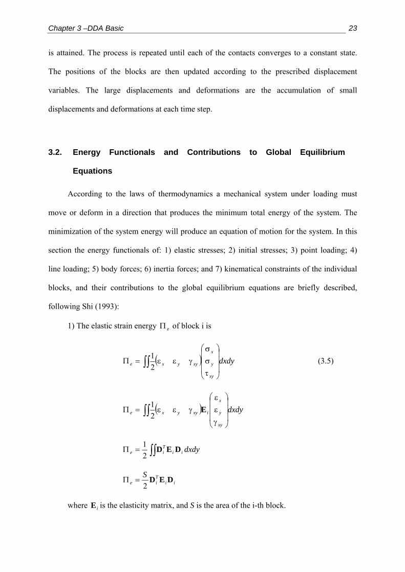
1) The elastic strain energy of block i is eΠ
( ) dxdy
xy
y
x
xyyxe⎟⎟⎟
⎠
⎞
⎜⎜⎜
⎝
⎛
τσσ
γεε=Π ∫∫ 21 (3.5)
( ) dxdy
xy
y
x
ixyyxe⎟⎟⎟
⎠
⎞
⎜⎜⎜
⎝
⎛
γεε
γεε=Π ∫∫ E21
∫∫=Π dxdyiiTie DED
21
iiTie
S DED2
=Π
where is the elasticity matrix, and S is the area of the i-th block. iE

Chapter 3 –DDA Basic 24
The derivatives are
iiTi
sirisiri
ers dd
Sdd
k DED∂∂∂
=∂∂Π∂
=22
2, 61 ,,s,r …= (3.5.1)
irs Sk E=
rsk forms a submatrix which is added to the sub-matrix in the global equation 66× iiK
2) The potential energy of the initial stresses σΠ of block i is
(3.6) ( )∫∫⎟⎟⎟⎟
⎠
⎞
⎜⎜⎜⎜
⎝
⎛
τ
σσ
γεε−=Πσ dxdy
xy
y
xo
o
xyyx0
{ }0σ−=ΠσTiSD
The derivatives are
{ }ri
Ti
rir d
Sd
f∂
σ∂=
∂Π∂
= σ 0D, 61 ,,r …= (3.6.1)
{ }0σ= Sf r
rf forms a submatrix which is added to 16× { }iF in the global equation.
3) The potential energy of the point loading { } is ⎭⎬⎫
⎩⎨⎧
=y
x
ff
F
(3.7) ( ) {FTD Ti
Ti
y
xp f
fvu −=
⎭⎬⎫
⎩⎨⎧
−=Π }
The derivatives are
{ }ryrx
ri
Ti
Ti
ri
pr tftf
ddf 21 +=
∂∂
=∂Π∂
−=FTD 61 ,,r …= (3.7.1)
rf forms a submatrix which is added to 16× { }iF in the global equation.
4) The potential energy of load distributed on a straight line from point to point
is
)y,x( 11
)y,x( 22

Chapter 3 –DDA Basic 25
(3.8.) ( ) { }∫∫ =⎭⎬⎫
⎩⎨⎧
−=Π1
0
1
0
ldt)t(ldt)t(F)t(F
vu Ti
Ti
y
xl FTD
where t is the parametric coefficient of the line equation, and l is the length of the line
segment between the end points.
The derivatives are
{ } )ldt)t((dd
f Ti
Ti
rr
lr ∫∂
∂=
∂Π∂
−=1
0
FTD 61 ,,r …= (3.8.1)
{ }∫=1
0
ldt)t(f Tir FT
rf forms a submatrix which is added to 16× { }iF in the global equation.
5) The potential energy of the of a constant body force ( )yx ff acting on the volume
of the i-th block is
(3.9) ( )⎭⎬⎫
⎩⎨⎧
−=⎭⎬⎫
⎩⎨⎧
−=Π ∫∫∫∫y
xTi
Ti
y
xw f
fdxdydxdy
ff
vu TD
given then ST =
⎟⎟⎟⎟⎟⎟⎟⎟
⎠
⎞
⎜⎜⎜⎜⎜⎜⎜⎜
⎝
⎛
=∫∫
00000000
00S
S
dxdyTi
⎟⎟⎟⎟⎟⎟⎟⎟
⎠
⎞
⎜⎜⎜⎜⎜⎜⎜⎜
⎝
⎛
−=Π
0000SfSf
x
x
Tiw D
The derivatives are
⎟⎟⎟⎟⎟⎟⎟⎟
⎠
⎞
⎜⎜⎜⎜⎜⎜⎜⎜
⎝
⎛
=
⎟⎟⎟⎟⎟⎟⎟⎟
⎠
⎞
⎜⎜⎜⎜⎜⎜⎜⎜
⎝
⎛
∂∂
=∂Π∂
−=
0000
0000
SfSf
)
SfSf
(dd
f
x
x
x
x
Ti
riri
wr D 61 ,,r …= (3.9.1)
rf forms a submatrix which is added to 16× { }iF in the global equation.
Chapter 3 –DDA Basic 26
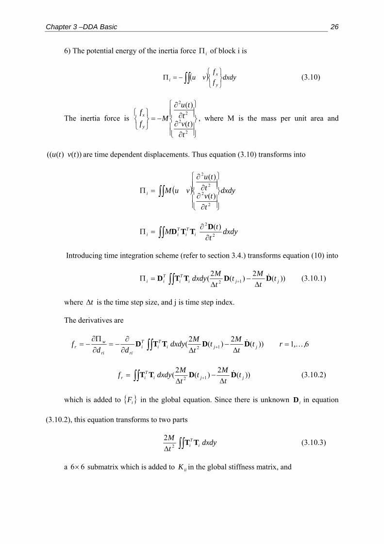
6) The potential energy of the inertia force iΠ of block i is
(3.10) ( ) dxdyff
vuy
xi
⎭⎬⎫
⎩⎨⎧
−=Π ∫∫
The inertia force is
⎪⎪⎭
⎪⎪⎬
⎫
⎪⎪⎩
⎪⎪⎨
⎧
∂∂∂
∂
−=⎭⎬⎫
⎩⎨⎧
2
2
2
2
)(
)(
ttv
ttu
Mff
y
x , where M is the mass per unit area and
are time dependent displacements. Thus equation (3.10) transforms into ))()((( tvtu
( ) dxdy
ttv
ttu
vuMi
⎪⎪⎭
⎪⎪⎬
⎫
⎪⎪⎩
⎪⎪⎨
⎧
∂∂∂
∂
=Π ∫∫2
2
2
2
)(
)(
∫∫ ∂∂
=Π dxdyt
tM iTi
Tii 2
2 )(DTTD
Introducing time integration scheme (refer to section 3.4.) transforms equation (10) into
))(2)(2( 12 jjiTi
Tii t
tMt
tMdxdy DDTTD
∆−
∆=Π ∫∫ + (3.10.1)
where is the time step size, and j is time step index. t∆
The derivatives are
))(2)(2( 12 jjiTi
Ti
riri
wr t
tMt
tMdxdy
ddf DDTTD
∆−
∆∂∂
−=∂Π∂
−= ∫∫ + 61 ,,r …=
))(2)(2( 12 jjiTir t
tMt
tMdxdyf DDTT
∆−
∆= ∫∫ + (3.10.2)
which is added to { in the global equation. Since there is unknown in equation
(3.10.2), this equation transforms to two parts
}iF iD
∫∫∆dxdy
tM
iTi TT2
2 (3.10.3)
a submatrix which is added to in the global stiffness matrix, and 66× iiK

Chapter 3 –DDA Basic 27
)(2ji
Ti tdxdy
tM DTT∫∫∆
(3.10.4)
a submatrix which is added to 16× { }iF in the global equation.
7) Displacement constraint at a point.
For a fixed point in a block the displacements are . Two stiff springs are
assigned in the x and y direction respectively. The stiffness of the springs is p and the spring
forces are .
{ }0=⎭⎬⎫
⎩⎨⎧
)y,x(v)y,x(u
⎭⎬⎫
⎩⎨⎧
−=⎭⎬⎫
⎩⎨⎧
vu
pff
y
x
The potential energy of the spring mΠ is
iiTi
Tim
pvu
)vu(p DTTD22
=⎭⎬⎫
⎩⎨⎧
=Π (3.11)
The derivatives are
iiTi
Ti
sirisiri
mrs dd
pdd
k DTTD∂∂∂
=∂∂Π∂
=22
2 61 ,,s,r …=
(3.11.1) iTirs pk TT=
rsk forms a submatrix which is added to in the global stiffness matrix. 66× iiK
3.3. Block System Kinematics and Contacts
Block system kinematics in DDA is constrained by the no tension no penetration
condition between the blocks, mathematically described by a system of inequalities. As
pointed out by Shi (1993) the minimization of total potential energy with inequality
constraints is a non linear programming problem of high difficulty. However, when the block

Chapter 3 –DDA Basic 28
system moves or deforms the blocks are in contact only along boundaries and the non
penetration inequalities can be transformed into equations when the blocks are in contact.
The equations can be imposed on the global equation by adding numeric penalties to
lock the movement in one or two directions. If two blocks have a tensile contact force
between them, they will separate when the locks are removed. The global equations have to
be solved repeatedly while selecting the lock position. Using this method the block system
with tension and penetration can be corrected, by selection of lock position, until the
fundamental constraints are satisfied.
3.3.1. Distance between two blocks
Two blocks meet at the next time step only if they are near at during the current time
step. The distance between blocks i and j is defined is the minimum distance ηij of any point
pair P1(x1,y1) of block i and P2(x2,y2) of block j (Figure3.1):
{ }jiij ByxByxyyxx ∈∀∈∀−+−= ),(,),()()(min 22112
122
12η (3.12)
where ∀ denotes “for all”.
Bi
(x1, y1)
(x2, y2)Bj
ηij
P1
P2 P3
Figure 3.1. Distance of two blocks (after Shi, 1993)
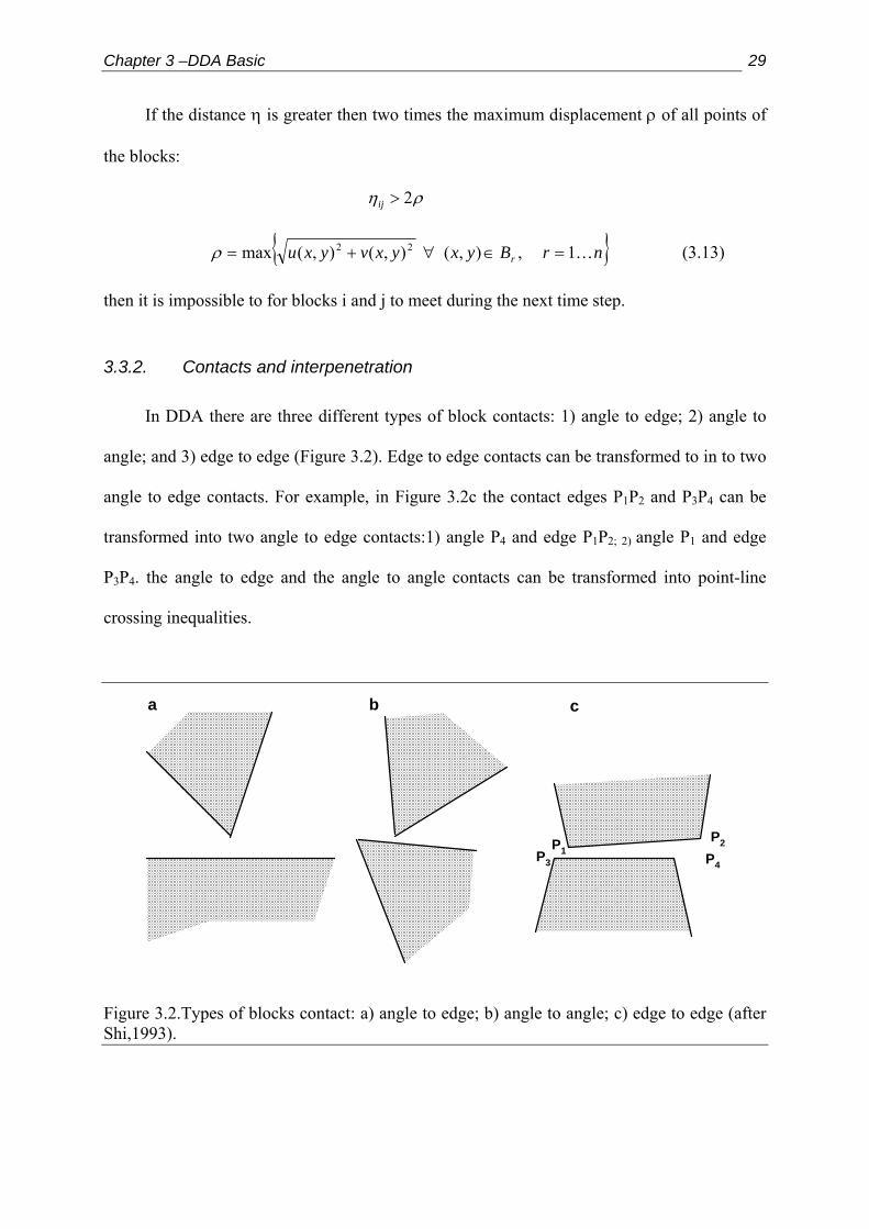
Chapter 3 –DDA Basic 29
If the distance η is greater then two times the maximum displacement ρ of all points of
the blocks:
ρη 2>ij
{ }nrByxyxvyxu r …1,),(),(),(max 22 =∈∀+=ρ (3.13)
then it is impossible to for blocks i and j to meet during the next time step.
3.3.2. Contacts and interpenetration
In DDA there are three different types of block contacts: 1) angle to edge; 2) angle to
angle; and 3) edge to edge (Figure 3.2). Edge to edge contacts can be transformed to in to two
angle to edge contacts. For example, in Figure 3.2c the contact edges P1P2 and P3P4 can be
transformed into two angle to edge contacts:1) angle P4 and edge P1P2; 2) angle P1 and edge
P3P4. the angle to edge and the angle to angle contacts can be transformed into point-line
crossing inequalities.
a b c
P1P3
P2
P4
Figure 3.2.Types of blocks contact: a) angle to edge; b) angle to angle; c) edge to edge (after Shi,1993).

Chapter 3 –DDA Basic 30
An edge and an angle are defined to be in contact if the distance from angle to edge is
less than ρ and if there is no overlapping when angle vertex translates to the edge without
rotation. In Figure 3.3a there is overlapping when non rotational translation is made, and
therefore the angle and the edge are not in contact.
Two angles are defined to be in contact if the distance between the vertices is less than
� and if there is no overlapping when angle vertex translates to the edge without rotation until
the vertices coincide. In Figure 3.3b there is overlapping and therefore the two angles are not
in contact .The concept of contact is extremely important: if there is no penetration at the
contacts there is no penetration in the whole block system.
P1
P2
P3
O
P2
P3
O
a
P1
P2
P1
b
Figure 3.3 Contact conditions: a) overlapping angle and edge; b) overlapping angles (modified after Shi,1993)
3.3.3. Energy functional of a stiff contact
If a vertex of block i with coordinates is penetrating an edge of block j with
vertices and , the penetration distance d can be denoted as
)y,x( 11
)y,x( 22 )y,x( 33
⎟⎟⎟
⎠
⎞
⎜⎜⎜
⎝
⎛++=
++++++
∆=
33
32
11
33
22
11
0
3333
3222
1111
111
111
1
111
vxvxvx
yuyuyu
Sl
vyuxvyuxvyux
ld (3.14)
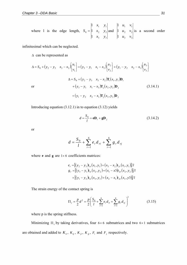
Chapter 3 –DDA Basic 31
where l is the edge length,
33
22
11
0
111
yxyxyx
S = and
33
22
11
111
vuvuvu
is a second order
infinitesimal which can be neglected.
∆ can be represented as
( ) ( ) (⎭⎬⎫
⎩⎨⎧
−−+⎭⎬⎫
⎩⎨⎧
−−+⎭⎬⎫
⎩⎨⎧
−−+=∆3
31221
2
23113
1
123320 v
uxxyy
vu
xxyyvu
xxyyS )
or
( ) ( )
( ) (
( ) ( jj
jj
ii
y,xxxyy
y,xxxyy
y,xxxyyS
DT
DT
DT
331221
223113
1123320
−−+
−−+ )
)
−−+=∆
(3.14.1)
Introducing equation (3.12.1) in to equation (3.12) yields
jilS
d gDeD ++= 0 (3.14.2)
or
∑∑==
++=6
1
6
1
0
rrjr
rrir dgde
lS
d
where and g are coefficients matrices: e 61×
( ) ( ) ( ) ( )[ ]( ) ( ) ( ) ( )[ ]( ) ( ) ( ) ( )[ ] ly,xtxxy,xtyy
ly,xtxxy,xtyygly,xtxxy,xtyye
rr
rrr
rrr
3
3
321233121
222122113
1122311132
−+−+
−+−=−+−=
The strain energy of the contact spring is
26
1
6
1
02
22 ⎟⎟⎠
⎞⎜⎜⎝
⎛++==Π ∑∑
== rrjr
rrirc dgde
lSpdp (3.15)
where p is the spring stiffness.
Minimizing by taking derivatives, four cΠ 66× submatrices and two submatrices
are obtained and added to , , , , and respectively.
16×
iiK ijK jiK jjK iF jF

Chapter 3 –DDA Basic 32
26
1
22
2 ⎟⎟⎠
⎞⎜⎜⎝
⎛∂∂∂
=∂∂Π∂
= ∑=r
rirsirisiri
krs de
ddp
ddk (3.16)
srrs epek = 61 ,,s,r …=
rsk is a submatrix which is added to in the global equation. 66× iiK
( ) ( )∑∑==∂∂
∂=
∂∂Π∂
=6
1
6
1
22
2 rrjr
rrir
sjrisjri
krs dgde
ddp
ddk (3.17)
srrs gpek = 61 ,,s,r …=
rsk is a submatrix which is added to in the global equation. 66× ijK
( ) ( )∑∑==∂∂
∂=
∂∂Π∂
=6
1
6
1
22
2 rrjr
rrir
sirjsirj
krs dgde
ddp
ddk (3.18)
srrs epgk = 61 ,,s,r …=
rsk is a submatrix which is added to in the global equation. 66× jiK
26
1
22
2 ⎟⎟⎠
⎞⎜⎜⎝
⎛∂∂∂
=∂∂Π∂
= ∑=r
rjrsjrjsjrj
krs dg
ddp
ddk (3.19)
srrs gpgk = 61 ,,s,r …=
rsk is a submatrix which is added to in the global equation. 66× jjK
(∑=∂
∂−=
∂Π∂
−=6
1
0
rrir
riri
kr de
dlpS
df ) (3.20)
lepS
f rr
0−= 61 ,,r …=
rf is a submatrix which is added to in the global equation. 16× iF
(∑=∂
∂−=
∂Π∂
−=6
1
0
rrjr
rirj
kr dg
dlpS
df ) (3.21)
lgpS
f rr
0−= 61 ,,r …=
rf is a submatrix which is added to in the global equation. 16× jF

Chapter 3 –DDA Basic 33
3.3.4. Limitations of DDA stiff contact formulation
In DDA the contact stiffness is determined at the beginning of the computation and is
kept constant throughout the entire calculation. In deforming rock masses some deformation
is taking place at the contacts. Deformation of the contacts and subsequent changes of contact
areas and angles are not accounted by DDA. This deformation consumes energy, which is not
accounted by as well.
αα
θ
P
y
x
α
α
x
y
P
θ
0
0
Figure 3.4. A wedge loaded by normal and tangential forces at the apex (after Timoshenko and Goodier, 1951)
Timoshenko and Goodier (1951) describe the stress concentration at wedge (similar to a
DDA edge) loaded by a normal and tangential forces at the apex (Figure 3.4). The radial
stress concentration due to normal loading within the wedge is given by:
)2sin21(
cos
αα
ασ+
−=r
Pr (3.22a)
The tangential stress concentration due to normal loading within the wedge is given by:
)2sin21(
cos
αα
ασ−
−=r
Pr (3.22b)

Chapter 3 –DDA Basic 34
Clearly the stress concentration is a function of the geometrical factor )2sin
21(
1
αα ±=k ,
which is related to the vertex angle 2α. During deformation this angle is expected to change,
and so does the factor k. This factor bares similarity to contact stiffness, relates stress to force,
and can be transformed into a formal stiffness, which relates force to displacement, by the
application of Hooke’s law. Therefore, it can be assumed that contact stiffness is expected to
change during deformation as well.
DDA version used in this research assumes first order displacement function, resulting
in homogenously deformable elements. In order to accommodate a realistic contact
formulation, as described above, high order displacement functions should be used. High
order displacement functions were implemented into DDA by various investigators (refer to
Hsiung, S-M, 2001), however the contact stiffness was modeled using constant stiffness
springs. Amadei et al., (1996) reformulated the contact scheme by substituting the stiff
contacts by Lagrangian multipliers, which are constantly updated trough the computational
cycles. However, this technique is essentially numerical with vague physical meaning.
Future development of the DDA should account for this deficiency, if more accurate
description of deformation is desired.
3.4. Time Integration Scheme
DDA time integration scheme adopts the Newmark (1959) approach, which for a single
degree of freedom can be written in the following manner:
11
122
1
)1(
)21(
++
++
∆+∆−+=
∆+∆−+∆+=
iiii
iiiii
ututuu
utututuu
γγ
ββ (3.23)

Chapter 3 –DDA Basic 35
where , , and are acceleration, velocity, and displacement respectively, is the
time step,
u u u t∆
β and γ are the collocation parameters defining the variation of acceleration over
the time step. Unconditional stability of the scheme is assured for 5.02 ≥≥ γβ . DDA
integration scheme uses 5.0=β and 1=γ , thus setting the acceleration at the end of the time
step to be constant over the time step. This approach is implicit and unconditionally stable.
Along with unconditional stability this set of collocation parameters assures a high
algorithmic damping (Wang et al., 1996). This phenomenon is commonly observed when
numerical methods are used to analyze the dynamic behavior of elastic systems.
Consider a two block system, as depicted in Figure 3.1. The equilibrium solution of the
vertical stress at the centroid of the upper block is MPay 01226.0=σ . The effect of
algorithmic damping can be seen in Figure 3.2a, which is a plot of the vertical stress at the
centroid of the upper block versus time. DDA solution equilibrates with time, as is clearly
seen for the case of contact spring stiffness . For higher contact stiffness
the solution further stabilizes.
mMNg /10500 6⋅=
The effect of increased contact stiffness is seen in Figure 3.2b, which is a plot of the
relative numeric error versus time. The relative numeric error is defined as:
100(%)*
⋅−
=y
yyne
σσσ
(3.21)
where yσ is equilibrium solution vertical stress and is the numerically calculated
vertical stress; both are taken at the upper block centroid. It is clearly seen that algorithmic
damping is active for the lower contact stiffness, where the numeric error is reduced from
initial value of 3% to 0.3% over 20 time steps. As contact stiffness approaches infinity the
numeric error declines, as low as 0.01% for contact stiffness of . Thus, it can
be concluded that DDA solution approaches equilibrium solution faster with increased contact
stiffness.
*yσ
mMN /10100 9⋅

Chapter 3 –DDA Basic 36
Riding Block
Base Block
1m
2m
c
Figure 3.5. Two block system.
The origin of the initial error is the contact force perturbation at the initial time step of
the computation, at gravity turn-on. As shown by Doolin and Sitar (2002) initial contact force
perturbation is inversely proportional to the time step size. This effect can bee seen in Figure
3.3, which shows the DDA solution (Fig. 3.3a) and the numeric error (Fig. 3.3b) of the
previously described problem. For a time step of sec05.0=∆t the initial perturbation is of
approximately 4%. Reducing the time step size, up to magnitude order scale, results in higher
initial error. However, the convergence of DDA solution is markedly enhanced by time step
size reduction, down to a numeric error of 0.005%.
From the above discussion, it is clear that the accuracy of DDA solution is governed by
two parameters: 1) time step size; 2) contact stiffness. The most accurate solution is attained
for smaller time step size and higher values of contact stiffness. This effect will be discussed
further in the following chapters.

Chapter 3 –DDA Basic 37
3.5. DDA Numeric Implementation
Computer implementation of DDA allows control over the analysis procedure through a
set of user specified control parameters:
1. Dynamic control parameter (k01) – defines the type of analysis required, from
quasi-static to fully dynamic. For quasi-static analysis the velocity of each block at
the beginning of each time step is set to zero, 001=k . In case of dynamic analysis
the velocity of each block at the end of a time step is fully transferred to the next
time step, . Different values from 0 to 1 correspond to different degrees of
inter step velocity transfer, comparable to damping or energy dissipation. For
example, for an input value of
101=k
95001 .k = the velocity in the beginning of each time
step is 5% lower then the terminal velocity at the previous time step.
2. Penalty value (g0) – is the stiffness of the contact springs used to enforce
contact constraints between blocks.
3. Upper limit of time step size (g1) – the maximum time interval that can be
used in a time step, should be chosen so that the assumption of infinitesimal
displacement within the time step is satisfied.
4. Assumed maximum displacement ratio (g2) – the calculated maximum
displacement within a time step is limited to an assumed maximum displacement in
order to ensure infinitesimal displacements within a time step. The assumed
maximum displacement is defined as )y()g(U max 22 ⋅= , where y is the length of the
analysis domain in the y-direction. This parameter is also used to detect possible
contacts between blocks: if the distance between separated vertices or edges of
neighboring blocks is less than )y()g(. 2252 ⋅ then the blocks are in contact. If
is too large there are too many unnecessary contacts, if is too small unrealistic
inter-block penetration can occur.
2g
2g

Chapter 3 –DDA Basic 38
0.0112
0.0116
0.012
0.0124
0.0128
0.0132
Stre
ss (
MP
a)
g0 = 50*106 N/m
0.1 0.2 0.3 0.4 0.5 0.6 0.7 0.8 0.9 1Time (sec)
0.01
0.1
1
10
e n (%
)
g0 = 50*106 N/m
g0 = 500*106 N/m
g0 = 1*109 N/m
g0 = 500*106 N/m
g0 = 1*109 N/m
g0 = 10*109 N/m
g0 = 100*109 N/m
Figure 3.6. DDA results for the two block system: for a time step size of g1 = 0.005 sec a) vertical stress at the centroid of the upper block for different values of contact stiffness; b) relative numeric error for different values of contact stiffness.

Chapter 3 –DDA Basic 39
0.01
0.011
0.012
0.013
0.014
Stre
ss (
MP
a)
0.015
0.1 0.2 0.3 0.4 0.5 0.6 0.7 0.8 0.9 1Time (sec)
0.001
0.01
0.1
1
10
100
e n (%
)g1 = 0.05 sec
g1 = 0.025 sec
g1 = 0.01 sec
g1 = 0.005 sec
g1 = 0.05 sec
g1 = 0.025 sec
g1 = 0.01 sec
g1 = 0.005 sec
Figure 3.7. DDA results for the two block system for contact stiffness of g0 = 50·106 N/m: a) vertical stress at the centroid of the upper block for different values of time step size (g1) ; b) relative numeric error for different values of time step size (g1).

Chapter 4 – Validation of DDA using shaking table model 40
Chapter 4 – Validation of DDA Using Analytical Solutions and Shaking Table Experiments
4.1. Introduction
Realistic simulation of a large number of individually deformable particles/blocks
requires the application of DEM, such as the Distinct Element Method (Cundall, 1971) or the
Discontinuous Deformation Analysis (Shi, 1988). Ever-growing popularity of numerical
schemes, in hand with availability of computing power eases the application of computer-
based methods. However, successful application of numerical methods to large-scale
engineering problems requires rigorous validation of these methods using analytical solutions,
laboratory scale models, and case studies.
Yeung (1991) and MacLaughlin (1997) tested the accuracy of DDA for applications
ranging from tunneling to slope stability, using problems for which analytical or semi-
analytical solutions exist. Doolin and Sitar (2002) explored the kinematics of a block on an
incline for sliding distances of up to 250 meters. Hatzor and Feintuch (2001) validated DDA
using direct dynamic input. Analytical integration of sinusoidal functions of increasing
complexity was compared to displacements prescribed by DDA for a single block on an
incline subjected to the same acceleration functions as integrated analytically.
The necessity for DDA validation using analytical solutions is evident if the method is
to be adopted by the engineering profession. However, analytical solutions are only valid for
the inherent underlying simplifying assumptions. This limitation can be overcome by
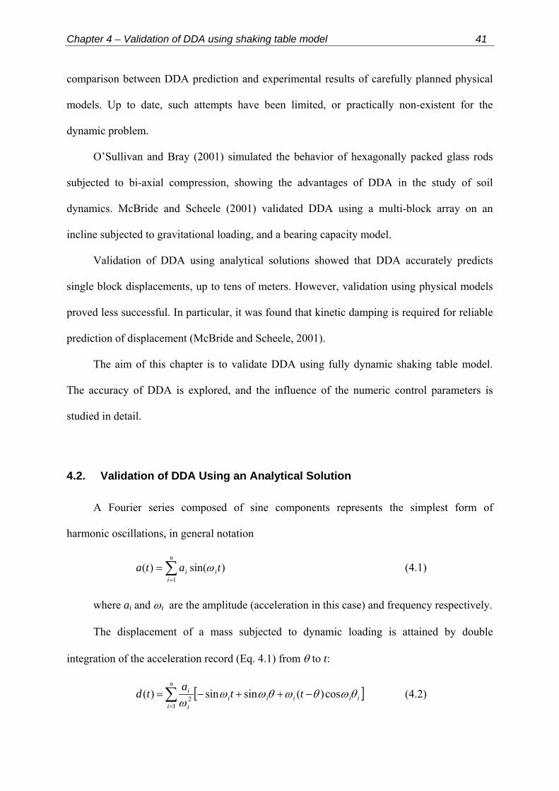
Chapter 4 – Validation of DDA using shaking table model 41
comparison between DDA prediction and experimental results of carefully planned physical
models. Up to date, such attempts have been limited, or practically non-existent for the
dynamic problem.
O’Sullivan and Bray (2001) simulated the behavior of hexagonally packed glass rods
subjected to bi-axial compression, showing the advantages of DDA in the study of soil
dynamics. McBride and Scheele (2001) validated DDA using a multi-block array on an
incline subjected to gravitational loading, and a bearing capacity model.
Validation of DDA using analytical solutions showed that DDA accurately predicts
single block displacements, up to tens of meters. However, validation using physical models
proved less successful. In particular, it was found that kinetic damping is required for reliable
prediction of displacement (McBride and Scheele, 2001).
The aim of this chapter is to validate DDA using fully dynamic shaking table model.
The accuracy of DDA is explored, and the influence of the numeric control parameters is
studied in detail.
4.2. Validation of DDA Using an Analytical Solution
A Fourier series composed of sine components represents the simplest form of
harmonic oscillations, in general notation
(4.1) ∑=
=n
iii tata
1)sin()( ω
where ai and ωι are the amplitude (acceleration in this case) and frequency respectively.
The displacement of a mass subjected to dynamic loading is attained by double
integration of the acceleration record (Eq. 4.1) from θ to t:
[ ]∑=
−++−=n
iiiiii
i
i ttatd1
2 cos)(sinsin)( θωθωθωωω
(4.2)

Chapter 4 – Validation of DDA using shaking table model 42
where θ is the time at which yield acceleration ay is attained.
Goodman and Seed (1965) showed that for frictional sliding of a single block on a plane
inclined by α degrees, where cohesion along the sliding plane is zero, the down slope
horizontal yield acceleration (ay) is
ga dy )tan( αφ −= (4.3)
Up slope horizontal yield acceleration is
ga dy )tan( αφ += (4.4)
where φd is the displacement dependent friction angle. It is apparent that up slope
motion requires significantly higher accelerations, which in most cases preclude up slope
displacement.
Hatzor and Feintuch (2001) showed that for an acceleration function consisting of sum
of three sines DDA prediction is accurate within 15% of the analytic solution without
application of damping, provided that the numeric control parameters g1, g2 are carefully
optimized. Moreover, they argued that the influence of higher order terms in a series of sine
function is negligible. Hatzor and Feintuch demonstrated their validation for arbitrary selected
constants, a1 = ω1 = 1, a2 = ω2 = 2, a3 = ω3 = 3. The prescribed values produce a low
frequency dynamic input assuring a nearly constant block velocity, which was attained at the
beginning of the analysis (ca. 20% of elapsed time).
In order to attain a better understanding of the frequency effect upon the numerical
solution we have extended the analysis to higher frequencies, constraining the peak horizontal
acceleration to 0.15g. A typical input motion of sum of three sines is presented in Figure 4.1a.
The analysis was performed for a single block resting on a plane inclined α = 150 to the
horizontal. The block material properties were: density = 2700 kg/m3, E = 5000 MPa, and ν =
0.25. The friction angle of the sliding plane was set to φ = 150, thus the yield acceleration (ay
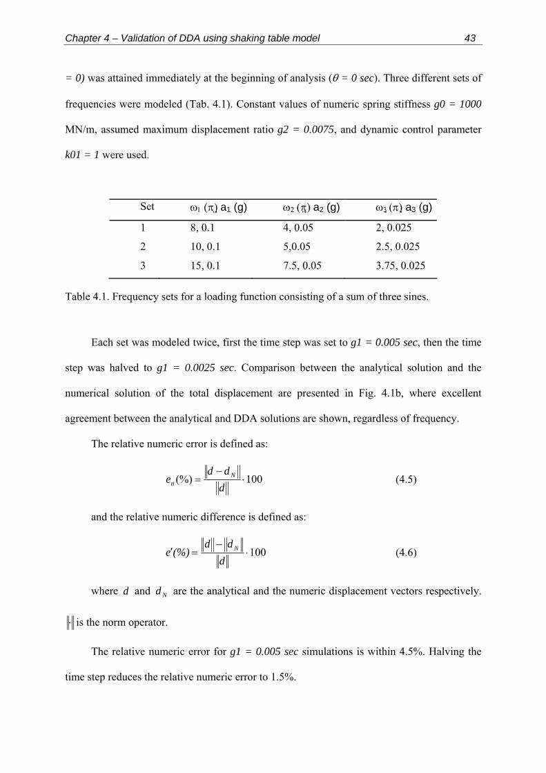
Chapter 4 – Validation of DDA using shaking table model 43
= 0) was attained immediately at the beginning of analysis (θ = 0 sec). Three different sets of
frequencies were modeled (Tab. 4.1). Constant values of numeric spring stiffness g0 = 1000
MN/m, assumed maximum displacement ratio g2 = 0.0075, and dynamic control parameter
k01 = 1 were used.
Set ω1 (π) a1 (g) ω2 (π) a2 (g) ω3 (π) a3 (g)
1 8, 0.1 4, 0.05 2, 0.025
2 10, 0.1 5,0.05 2.5, 0.025
3 15, 0.1 7.5, 0.05 3.75, 0.025
Table 4.1. Frequency sets for a loading function consisting of a sum of three sines.
Each set was modeled twice, first the time step was set to g1 = 0.005 sec, then the time
step was halved to g1 = 0.0025 sec. Comparison between the analytical solution and the
numerical solution of the total displacement are presented in Fig. 4.1b, where excellent
agreement between the analytical and DDA solutions are shown, regardless of frequency.
The relative numeric error is defined as:
100(%) ⋅−
=ddd
e Nn (4.5)
and the relative numeric difference is defined as:
100⋅−
=′d
dd(%)e N (4.6)
where and are the analytical and the numeric displacement vectors respectively. d Nd
⋅ is the norm operator.
The relative numeric error for g1 = 0.005 sec simulations is within 4.5%. Halving the
time step reduces the relative numeric error to 1.5%.

Chapter 4 – Validation of DDA using shaking table model 44
0 1 2 3 4 5 6Time (sec.)
0
0.1
0.2
0.3
0.4
0.5
0.6
0.7
0.8
Dis
plac
emen
t (m
.)
ω1 = 8π = 2ω2 = 4ω3
ω1 = 10π = 2ω2 = 4ω3
ω1 = 15π = 2ω2 = 4ω3
-0.2
-0.1
0
0.1
0.2Ac
cele
ratio
n (g
)a(t) = 0.1sin8πt + 0.05sin4πt + 0.025sin2πt a
bFull Symbols - DDA output, g1 =0.0025secEmpty Symbols - DDA output, g1 =0.005secFull Lines - Analytical Solution
Figure 4.1. a) the loading function a(t) = a1sin(ω1t) + a2sin(ω2t)+ a3sin(ω3t); b) comparison between analytical and DDA solution for block displacement subjected to a loading function consisting of a sum of three sines. All DDA simulations for:g0 = 1*109 N/m; g2 = 0.0075; block elastic modulus E = 5000*106 N/m. All input motions are for ω1= 2ω2 = 4ω3.

Chapter 4 – Validation of DDA using shaking table model 45
100 1000 10000Numeric spring stiffnes (106 N/m)
0.1
1
10
100
1000
10000
e (%
)
g1 = 0.0025 g2 = 0.0075g1 = 0.005 g2 = 0.0075g1 = 0.0075 g2 = 0.01g1 = g2 = 0.01
a
0.01 0.02 0.03 0.04 0.05∆t / Ti
0.1
1
10
100
1000
e (%
)
g0 (106 N/m)1002505001000
b
Figure 4.2. Sensitivity analysis of the DDA numeric control parameters. Relative numeric error of ultimate displacement prediction as a function of: a) contact spring stiffness; b) time step size (∆t) normalized to input motion frequency (Ti).

Chapter 4 – Validation of DDA using shaking table model 46
The interrelationship of the numeric control parameters was further investigated using
the input function of set 2 (Table 4.1). Figure 4.2 shows the dependence of the numeric error
on the choice of the numeric control parameters g1, g2 and the numeric spring stiffness g0
(the penalty value). It is found that for an optimized set of g1and g2 (g1 = 0.0025 sec and g2
= 0.0075) the DDA solution is not sensitive to the penalty value, which can be changed over a
range of two orders of magnitude, from 100×106 N/m to 5000×106 N/m. Within this range the
numeric error never exceeds 10% and in most cases approaches the value of 1%. For values
lower than 50×106 N/m block penetration occurs. Stiffer contact springs reduce the magnitude
of displacement until a certain minimum is reached. Further increase in the spring stiffness
results in an introduction of a large numeric error into the DDA solution.
Departing from the optimal g1, g2 combination results in increased sensitivity of the
DDA solution to the penalty value. The departure from the analytical solution occurs at lower
penalty values with increasing time step size.
Examining the optimal time step size (Fig. 4.2b) shows that time step optimization is
not a simple procedure. It is clear that highest accuracy is attained for a small time step – high
stiffness combination. However, enlargement of the time step size produces a different
response of the mechanical system: for higher stiffness values the numeric error tends to
grow, while for the lower ones it tends to decrease. Thus, an optimal combination is not easily
defined: the lowest numeric error (e = 0.6%) is attained for the following combination ∆t/Ti =
0. 0375 and g0 = 250×106 N/m. For the same time step size the errors for g0 = 500×106 N/m
and g0 = 1000×106 N/m are of an order of magnitude larger. However, the numerical stability
of DDA is assured regardless of the contact stiffness when time step size is taken sufficiently
low.
Chapter 4 – Validation of DDA using shaking table model 47
4.3. Validation of DDA by Shaking Table Experiments
It has been shown that there is a very good agreement between the DDA and analytic
solutions for the block on an incline problem. However, the analytical solution is only an
approximation to the physical problem with various simplifying assumptions including:
perfectly rigid block, constant friction, and complete energy conservation. Comparison
between DDA results and physical modeling can help us probe into the significance of these
assumptions. In the following section validation of DDA using a physical model of a block on
an incline subjected to dynamic loading is described.
4.3.1. Experimental setting
The physical modeling used in this research was performed by Wartman et al., (2003) at
the Earthquake Simulation Laboratory of the University of California at Berkeley. The tests
were performed on a large hydraulic driven shaking table, producing accurate, well
controlled, and repeatable motions to frequencies up to 14 Hz. The table was driven by a
222.4 kN (50 kip) force, 15.24 cm (6 in.) stroke range hydraulic actuator manufactured by
MTS. The system was closed loop servo controlled. A Hewlett Packard 33120A arbitrary
function generator produced the table command signal.
In this study sinusoidal input motion tests were used for validation. A typical sinusoidal
input motion is shown in Figure 4.3. The motion was ramped up linearly for 1.5 seconds to
insure shaking table stability, followed by full amplitude for duration of 2 seconds, and finally
ramped down for 1.5 seconds. Eight different tests were used for validation, the input
parameters of the dynamic loading functions are given in Table 4.2.
An inclined steel plane was fitted to the shaking table. The plane inclination was set to
11.370 during the rigid block tests. The steel rigid block was 2.54 cm (1 in.) thick, with area of
25.8 cm2 (4 in.2), and weight of 1.6 kg (3.5 lbs). Linear accelerometers were fitted on top of

Chapter 4 – Validation of DDA using shaking table model 48
the sliding block and the inclined plane. Displacement transducers measured the relative
displacement of the sliding block, and of the shaking table (Fig. 4.4).
A geotextile and a geomembrane were fitted to the face of the sliding block and the
inclined plane respectively. The static friction angle (φ) of the interface was determined using
tilt tests and a value of φ = 12.70±0.70 was reported. Kim et al., (1999) found that the friction
angle of the geotextile – geomembrane interface exhibited pronounced strain rate effects, and
reported an increase by 20% over one log-cycle of strain rate.
Wartman (2003) showed that the friction angle of the interface was controlled by two
factors: 1) amount of displacement; and 2) sliding velocity. The back-calculated friction angle
for the range of velocities and displacements measured was between φ = 140 - 190 (refer to
Fig. 4.5).
The DDA version used in this research accepts a constant value of friction angle.
Therefore a single friction angle (φav) value must be chosen for validation. The value of φav
was determined as follows. First, the measured displacement of the block was differentiated
with respect to time and hence the velocity record was attained. Next, the velocity content for
the duration of the test was computed. For example, the test of 2.66 Hz input motion
frequency showed that the upper bound velocity was below 10 cm/sec, refer to Figure 4.6a.
This value was attained only for short periods of time during the test. The velocity content
chart (Fig. 4.6b) shows that 80% of the velocities fall under the value of 3 cm/sec. Taking the
value of 3 cm/sec as upper bound, the corresponding friction angle is φav < 17o. The 50%
value corresponds to friction angle of φav = 16o. This value was chosen for DDA analysis.

Chapter 4 – Validation of DDA using shaking table model 49
0 1 2 3 4Time (sec.)
5
-0.3
-0.2
-0.1
0
0.1
0.2Ac
cele
ratio
n (g
)
Figure 4.3. Sinusoidal input motion for the shaking table experiment: 2.66 Hz frequency (Test 1 at Table 4.2).
Test ω (Hz) dT (cm) dB (cm) ah (g)
1 2.66 0.889 5.367 0.28
2 4 0.559 6.604 0.25
3 5.33 0.305 3.341 0.19
4 6 0.254 3.647 0.19
5 6.67 0.254 3.410 0.22
6 7.3 0.228 3.353 0.22
7 8 0.228 3.937 0.23
8 8.66 0.019 2.882 0.21
Table 4.2. Shaking table model summary: ω is the input motion frequency, dT is the shaking table displacement, dB is relative block displacement, and ah is maximum horizontal table acceleration.

Chapter 4 – Validation of DDA using shaking table model 50
3
4
114.3 cm (45 in)
No. Instrument Direction of Measurement 1 accelerometer parallel to plane 2 accelerometer parallel to plane 3 accelerometer horizontal 4 displacement transducer horizontal 5 displacement transducer parallel to plane
Shaking Table
11.37o
121.9 cm (48 in)
Inclined Plane
Rigid Block
1
2 5
Figure 4.4. a) general view of the inclined plane and the sliding block (top); b) sliding block experimental setup and instrumentation location (bottom), from Wartman (1999).

Chapter 4 – Validation of DDA using shaking table model 51
0.001 0.01 0.1 1 10 100average sliding velocity (cm/sec)
12
14
16
18
20
frict
ion
angl
e (φ
)
0.24
0.28
0.32
0.36
fric
tion
coef
ficie
nt
near static
med. to large displ.
small displ. (< 0.13 cm)
Figure 4.5. Back analyzed friction angles shown as a function of average sliding velocity for rigid block tests, from Wartman (2003).

Chapter 4 – Validation of DDA using shaking table model 52
0 1 2 3 4 5Time (sec)
-4
-2
0
2
4
6
8
10
12D
isp
lace
men
t (cm
)
0 1 2 3 4 5 6 7 8 9 10Velocity (cm/sec)
0
50
100
150
200
250
Freq
uen
cy
0.2
0.4
0.6
0.8
1
Cum
ula
tive
(*1
00 %
)
a
b
Displacement (cm)Velocity (cm / sec)
-4
-2
0
2
4
6
8
10
12
Vel
oci
ty (c
m/s
ec)
Figure 4.6. The 2.66 Hz sinusoidal input motion test: a) displacement derived velocity; b) velocity content.
Chapter 4 – Validation of DDA using shaking table model 53
4.4. DDA Prediction vs. Shaking Table Results
The numeric control parameters of DDA for this validation study were chosen
according to the guide-lines described in previous sections: penalty value g0 = 5*109 N/m,
time step size g1 = 0.0025 sec, assumed maximum displacement g2 = 0.005.
The 2.66 Hz motion is discussed here in detail and the results are shown in Figure 4.7.
Other seven tests yielded similar results, the final displacement errors for this tests are
summarized in Figure 4.9. For φav = 16o and k01 = 1 the numeric error is approximately 80%
(Fig. 4.8), but the ultimate displacement values are close, 0.055m measured displacement
compared to 0.093m of calculated solution, within the same order of magnitude. Introducing
some kinetic damping by reducing k01 below 1 improves the agreement between the
numerical estimate and physical test data.
Setting k01 = 0.98, corresponding to 2% velocity reduction, reduces the error to below
4%, and improves the tracking of the displacement history by DDA. Setting the k01 = 0.95
over damps the solution, resulting in a highly un-conservative displacement.
Plotting the numeric difference (%)e′ against input motion frequency (Fig. 4.9) shows
that in general DDA accuracy increases with higher frequencies, with an exception at 6 Hz.
For φav = 16o and k01 = 1 the numeric error is always conservative, with the exception of 6
Hz. Reducing k01 to 0.98 shows a similar effect for all frequencies, reducing the numeric
error below 10%. However, it should be mentioned that setting a constant friction angle for all
the analyzed tests introduces an un-conservative error. For input motions with essentially
similar peak acceleration, higher frequencies will result in lower block velocity. Given the
strain rate dependence of the sliding interface friction, lower velocities correspond to lower
friction angles. Thus, the accuracy of DDA could be improved with implementation of rate

Chapter 4 – Validation of DDA using shaking table model 54
dependent friction. This modification is beyond the scope of this study. Using the shaking
table results it may be concluded that a kinetic damping value of 2% should be proper for
realistic prediction of dynamic displacements.
4.4.1. Accuracy of DDA
The implicit formulation of DDA guaranties numerical stability regardless of time step
size. However, it does not guarantee accuracy. Where the time step is too large relative to the
numeric spring stiffness, loss of diagonal dominance and/or ill conditioning error may result,
interfering with convergence to an accurate solution.
The numeric implementation of DDA utilizes the SOR Gauss – Seidel equation solver.
The convergence of the SOR equation solver is guaranteed for diagonally dominant matrices:
∑>n
jijii KK ji ≠ (4.7)
Larger inertia terms on the diagonal of the global stiffness matrix increase the stability
of the computation. A small time step size is needed to increase the inertia terms, which are
inversely proportional to the square of time step. For small time steps (0.0025 sec) the
numeric error does not exceed 10% for increasing penalty values up to 5*1010 N/m; higher
penalty values, however, result in significant error as the off diagonal sub-matrices become
exceedingly large. Enlarging the time step results in reduction of inertia terms in the diagonal
sub-matrices. Therefore, for a given time step size the loss of diagonal dominance will occur
at lower penalty values.
Most of the error is accumulated at the beginning of the analysis and it declines with
time, a phenomenon known as algorithmic damping (refer to Wang et al., 1996 for elaborate
discussion of this phenomenon): typical to the Newmark implicit time integration scheme
(Figure 4.10). This behavior is observed here for all selected values of k01. In this study we
Chapter 4 – Validation of DDA using shaking table model 55
have limited the duration of the analysis to 5 seconds, in conjunction with the duration of the
shaking table experiment. Doolin and Sitar (2002) show that for a block on an incline problem
the relative error continues to decrease up to displacement of 250 m during 16 seconds of
sliding. Therefore, for computations involving larger time spans the error is expected to
decline as calculation proceeds, further improving solution accuracy.
When compared with analytical solutions for frictional sliding DDA is found to be
accurate. Therefore, it can be assumed that the contact formulation in DDA is equivalent to
the mathematical model for frictional sliding. The comparison with shaking table experiments
however implies that the contact formulation in DDA is not sufficiently accurate for modeling
physical friction. Consider for example the phenomenon of block “wobbling” during shaking
table experiments. In the numerical model the acceleration is applied as a concentrated body
force at the centroid of each block, whereas in the physical model block displacement is
induced by the motion of the shaking table. This motion causes block “wobbling” during
which physical contacts may open and close repeatedly. This process reduces the total energy
of the system and consequently the total down-slope displacement. Furthermore, the dynamic
formulation of DDA is essentially un-damped, friction being the main source of energy
consumption. In the physical model however mechanisms such as structural vibrations,
material damage along interface (ploughing), drag, heat etc. does take place during block
sliding. These processes are not modeled numerically and can be a second source of
discrepancy between the results of the numerical and physical models.
The only method available at present to simulate energy dissipation in DDA is by
reducing transferred velocity between time steps. In this study it is found that a reduction of
transferred velocity by 2% (k01 = 0.98) yields realistic prediction of block displacements,
further reduction of the dynamic control parameter yields un-conservatively small
displacements.
Chapter 4 – Validation of DDA using shaking table model 56
The numeric analyses show good agreement with the shaking table results, once kinetic
damping is applied. The reduction of the transferred velocity between time-steps is a numeric
adaptation not linked directly to a physical damping mechanism. Since DDA formulation is
essentially un-damped, viscous damping is not accounted for. Implementation of a dashpot
model in parallel with a contact spring (Voigt model) in order to simulate viscous damping in
DDA would be more appropriate. However, it is impossible to assign a correct damping
coefficient for the given problem a-priori. For problems of rock falls analyzed using DDA
with viscous damping (Chen et al, 1996; Shingi et al, 1997) the selection of the damping
coefficient was performed using trial and error procedure. We perform similar best “fitting”
by reducing the transferred velocity between time steps.
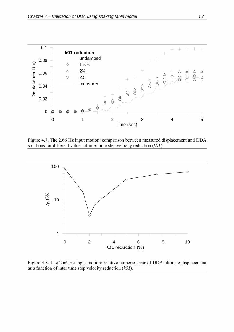
Chapter 4 – Validation of DDA using shaking table model 57
0 1 2 3 4Time (sec)
5
0
0.02
0.04
0.06
0.08
0.1
Dis
plac
emen
t (m
)
k01 reductionundamped1.5%2%2.5measured
Figure 4.7. The 2.66 Hz input motion: comparison between measured displacement and DDA solutions for different values of inter time step velocity reduction (k01).
0 2 4 6 8 10K01 reduction (%)
1
10
100
e n (
%)
Figure 4.8. The 2.66 Hz input motion: relative numeric error of DDA ultimate displacement as a function of inter time step velocity reduction (k01).

Chapter 4 – Validation of DDA using shaking table model 58
2 4 6 8 10Input motion frequency (Hz)
-120
-80
-40
0
40
e' (
%)
Conservative
Unconservative
k01 = 1
k01 = 0.98
Figure 4.9. Numeric difference of DDA ultimate displacement prediction as a function of input motion frequency.
0 1 2 3 4 5Elapsed time / Total time
1
10
100
1000
10000
e n (
%)
k01 = 1
0.985
0.98
0.975
Figure 4.10. The 2.66 Hz input motion: evolution over time of the DDA relative numeric error, for different values of the k01 parameter.

Chapter 4 – Validation of DDA using shaking table model 59
4.5. Conclusions
The results of the validation study show that DDA solution of an idealized system for
which an analytical solution exists, is accurate. The block contact algorithm in DDA is
therefore an accurate replication of the analytical model for frictional sliding.
The accuracy of DDA is governed by the conditioning of the stiffness matrix. The DDA
solution is accurate as long the chosen time step is small enough to assure diagonal
dominance of the global stiffness matrix.
Comparison between shaking table experiments and DDA calculation shows that the
DDA solution is generally conservative, over predicting block displacement. The main
sources of discrepancy between DDA and the physical model are the difference between the
numerical and actual behavior at contact points, and lack of a complex energy dissipation
algorithm in DDA.
For accurate displacement prediction a reduction of the dynamic control parameter
(k01) by 2% is recommended, for the block on a incline problem.
Implementation of viscous damping and strain/displacement dependent friction into
DDA can further improve the accuracy of the method.

Chapter 5 – Validation of DDA using a centrifuge model 60
Chapter 5 – Validation of DDA Using a Centrifuge Model of
a Jointed Rock Beam
5.1. Introduction
In the previous chapter, the accuracy of DDA was studied using a shaking table model
of a single block on an incline. It was shown that the accuracy of DDA is controlled by the
time step size, the contact spring stiffness, and the amount of kinetic damping. During sliding
the contacts between blocks, and consequently the stresses within the sliding block remained
unchanged. While this behavior is expected in sliding, it is certainly not expected during
deformation of a beam consisting of discontinuities. During the deformation of the jointed
beam some of the original contacts are expected to be destroyed while new contacts are
expected to form; consequently, block stresses are expected to change during ongoing
deformation. If DDA is to be applied to such problems, it should be validated using physical
model(s) where contacts and stresses are changing during deformation. In this chapter, DDA
is validated using centrifuge modeling of a multi-jointed beam.
Centrifuge modeling is based on the assumption of stress similarity. If acceleration of N
times earth gravity (g) is applied to a material of density ρ, the vertical stress (σv) at depth hm
of the model is given by:
mm,v Nghρ=σ (5.1)
In the prototype the vertical stress at depth hp is:

Chapter 5 – Validation of DDA using a centrifuge model 61
pp,v ghρ=σ (5.2)
Thus for vpvm σ=σ , and the scale factor is N. Since the centrifuge model
linearly scales the prototype, the displacements are also at scale factor of N. Strains, however,
have a scale factor of 1, and therefore the stress-strain curves in the model and the prototype
should be identical. This phenomenon is observed in centrifuge models up to peak strength
values. It is not usually possible to create residual shear planes with the same residual strength
as the prototype (Taylor, 1995). Talesnick and Hatzor (in prep.) showed that the concept of
dimensional scaling in the centrifuge, for situation including rock block interfaces, is not
warranted. Therefore, when a centrifuge model is comprised of discontinuous material stress
and displacement similarities with the prototype are not guaranteed.
pm hNh =
In this research centrifuge modeling was not performed in order to model a specific
engineering prototype, but rather to study the essential features of jointed beam deformation,
at various g levels.
5.2. Experimental Setting
Centrifuge modeling was performed by Dr. Mark Talesnick of the Department of
Geotechnical Engineering, Israel Institute of Technology (Technion). The tests were
performed using a beam type centrifuge with beam radius of 1.6 m, maximum payload
capacity of 5000kg, and maximum acceleration of 100g at the sample center.
5.2.1. Jointed beam model
The geometry of the model was of a beam made up of six blocks (Figure 5.1). The
blocks represent intersection of bedding planes with vertical joints, such as often found in
sedimentary rocks. Cubic blocks with edge length of L = 0.048m were cast from gypsum, and
the total beam span was S = 0.288m. The average block density was ρ = 998.1 kg/m3. The
Chapter 5 – Validation of DDA using a centrifuge model 62
elastic modulus of the blocks, found from uniaxial compression tests, was E = 3.2 GPa. The
friction between blocks was modeled using a 360 grit sand paper, glued to the contact faces of
individual blocks. The friction angle of the interface, determined at BGU using tilt test, was
φ = 35ο.
In order to ensure proper alignment of the blocks with respect to the sidewalls a
mechanical system depicted in Figure 5.1 was used. The system included a linear bearing that
resisted movements in directions other than the intended. A load cell was integrated into the
system in order to allow a specific thrust to be applied during the emplacement of the model.
The vertical movements of the block during the tests were recorded using six LVDT’s of
0.01mm resolution.
First a pre-stressing of the beam was performed to ensure beam stability at 0g level
(with reference to centrifuge axis). Then the acceleration was increased in-flight up to the
level of 12g. The beam deformed until stable configuration was attained, at all g levels tested.
5.3. DDA Model
5.3.1. A simple two-block system
Prior to comparison of centrifuge model and DDA results a study of a simple two-block
system subjected to gravitational loading was performed. Similar analysis, under somewhat
different boundary conditions was performed by Yeung (1991), showing good agreement
between the analytical and numerical solutions. In order to simplify the analysis and to
preclude vertical (shear) displacements at the abutments the two blocks were constrained by
assigning fixed points at base vertices, (Figure 5.3). The aim of this analysis was not to
reproduce analytical or semi-analytical solutions, but rather to study the behavior of the DDA
solution over time.

Chapter 5 – Validation of DDA using a centrifuge model 63
1
Instrumentation1. Load cell2. Pre-load screw3. LVDT4. Linear track
2
3
4
Blocks
Side wall blocks
Figure 5.1 Centrifuge model geometry and instrumentation (courtesy of M. Talesnick).
0.048m0.048m
fixed point
measurment point
Acceleration Field
f0 = 7.76kg
y
x
Figure 5.2 DDA model geometry.

Chapter 5 – Validation of DDA using a centrifuge model 64
DDA analysis was performed for the following material properties: E = 10 GPa, ν =
0.25, and ρ = 2.7·103 kg/m3. The block dimensions were: L = 2.5m, t =0.5m. The numerical
control parameters are: g0 = 1·109 MN/m, g1 = 0.001 sec, and g2 = 0.001. The dynamic
control parameter k01 was varied during the analysis.
Fixed point
S2
t
0 100 200 300 400Time Step (n.)
0
0.001
0.002
0.003
0.004
0.005
δ (m
)
0.006k01
10.990.970.950.90
1 0.98 0.96 0.94 0.92 0.9k01
0
100
200
300
400
n at
equ
ilibriu
m
a
b
Figure 5.3. DDA model of two block system with fixed base vertices: a) mid-span deflection (δ) as a function of time; b) number of time steps n required to attain equilibrium as a function of the dynamic control parameter (k01).
Chapter 5 – Validation of DDA using a centrifuge model 65
The dynamic behavior of the system is shown in Figure 5.3. The system attained
equilibrium position after deflection of m.0034550=δ . Algorithmic damping is evident, as
the initial perturbation, resulting from gravity turn-on, is dissipated with analysis progress.
The effect of dynamic “damping” through inter-step velocity reduction (k01) is apparent. By
reducing k01, the convergence to equilibrium position is enhanced, as the initial perturbation
decays with higher rate. For k01 = 1 equilibrium was attained after 320 time steps, reducing
the inter-step velocity by 1% (k01 = 0.99) resulted in equilibrium after 260 time steps. Further
reduction of k01 by 5% and 10% resulted in equilibrium after 120 and 40 time steps
respectively. This trend is clearly presented in Figure 5.3b.
Setting k01 = 0, namely eliminating inter-step velocity transfer, may be interpreted as
pseudo-static analysis. Under this condition changes in deflection evolved with time, from
initial zero position, until equilibrium solution is met after 240 time steps. Thus, for a system
attaining equilibrium, a slightly damped dynamic solution is more efficient numerically.
When analyzing a fully dynamic system the application of kinetic damping should be
preformed with care. In cases where the system is to attain equilibrium, or when the mode of
failure is independent of geometrical or mechanical constraints (such as in block sliding), the
application of kinetic damping is advantageous, since the solution converges rapidly.
However, when the mode of failure is determined by the block system geometry or by
mechanical properties, the application of kinetic damping is not without flaws. Consider, for
example, a single beam with multiple joints, the amount of deflection at mid-span is a
function of both joint spacing and friction along joints. Thus, for a beam of a given span but
with different joint spacing and friction, application of kinetic damping will not yield the
same effect on all solutions.
While for an equilibrating system kinetic damping will enhance the solution, for a non-
equilibrating system the solution will tend to retard with respect to the undamped solution.
Chapter 5 – Validation of DDA using a centrifuge model 66
Furthermore, two solutions of a damped non-equilibrating system are not equable, since the
solutions are at different stage of evolution.
5.3.2. A six block model
The initial geometry and boundary conditions in DDA for the jointed beam are given in
Figure 5.2. Material properties and friction along interfaces were modeled using the real
physical properties. Rigid abutments were modeled by assigning three fixed points to each
abutment block. The displacements were measured at 12 measurement points, symmetric with
respect to the centerline. Six measurement points were placed conforming to the exact
locations of the LVDT’s in the centrifuge model. The loading history was replicated in the
following manner: first the beam was pre-stressed using the initial value of the centrifuge
model, then the g level was changed every 240 time steps by 1g increments, up to acceleration
level of 12g, Figure 5.6.
5.3.3. Selection of numerical control parameters
In the previous chapter it was shown that the numeric control parameters are
interrelated. Accurate solutions were attained for properly chosen control parameters.
Therefore, prior to a comprehensive analysis of the centrifuge model by DDA, an initial
sensitivity analysis was performed. The time step size (g1), the maximum assumed
displacement (g2) and the dynamic control parameter (k01) were set to 0.0005 sec, 0.001 and
1 respectively. The contact stiffness between blocks (g0) was changed over three orders of
magnitude, from g0 = 10 MN/m to g0 = 1000 MN/m, and the displacements and stresses were
studied. The sensitivity analysis was performed at a loading level of 1g.
The results of the sensitivity study are presented in Figures 5.4a,b, and c. Figure 5.4a is
a plot of the vertical displacement profile, Figure 5.4b is a plot of the horizontal stress (σxx) at
the block centroids, and Figure 5.4c is the time history of beam deformation. Figure 5.4a

Chapter 5 – Validation of DDA using a centrifuge model 67
clearly shows that for low contact stiffness of g0 = 10 MN/m, the vertical movement of the
beam is excessive, with respect to the measured displacement (bold line). Furthermore, from
the deformation profile it is evident that the beam shears along abutments, as a single intact
beam. The extremely low stresses within the blocks confirm that arching (transfer of vertical
load to the abutments) within the beam is inactive, thus confirming the previous observation.
Increasing the contact stiffness to g0 = 100 MN/m reduces the vertical displacement, and
shows better stress prediction, however, the vertical displacements are still excessive, and the
stresses are low. Increasing the contact stiffness to g0 = 250 MN/m improves the stress
prediction, the displacements however are similar to those of g0 = 100 MN/m. The
deformation profile reveals that for both g0 = 100 MN/m and g0 = 250 MN/m the
displacement attains a maximum at the center of the beam and a minimum at the abutments,
implying that a mechanism of arching is active. The deformation is symmetric with respect to
the beam centerline.
Clearly, the amount of DDA predicted displacement, especially at the abutments, is
large with respect to the measured displacement. This discrepancy can be attributed to the
following factors:
1. Constant strain/stress elements (simply deformable blocks) – preclude the
development of stress concentrations within the blocks, and therefore of true
compressive arching, thus leading to increased displacements.
2. Representation of frictional interface – in the centrifuge model the frictional
interfaces, two facing sheets of sand-paper, are not infinitely thin, but rather
consists of a deformable element with a given thickness. In DDA the
discontinuity interface is infinitely thin, allowing only sliding or separation.

Chapter 5 – Validation of DDA using a centrifuge model 68
3. Rotational freedom – while the DDA model geometry can be regarded as
densely packed, the centrifuge model exhibits higher rotational freedom, due to
the nature of the frictional interfaces.
The rotation of the blocks during deformation in DDA is not evident, as opposed to the
rotations recorded in the centrifuge model. However, both centrifuge model and DDA predict
stability of the jointed beam after small amounts of deflection, through a build up of stresses.
For high contact stiffness, g0 ≥ 500 MN/m, the deformation profile shows unrealistic
behavior, loss of symmetry, and relative upward motion of blocks. For g0 = 500 MN/m the
stresses are accurate, whereas for g0 = 1000 MN/m the stresses are excessively high.
Time histories (Figure 5.4c) reveal that for all values of contact stiffness the beam
attains equilibrium position. The number of time steps until equilibrium is reached is smaller
for higher values of contact stiffness. Similar effect was shown by the simple two-block
example of Chapter 3. For g0 ≥ 500 MN/m equilibrium is attained after 60 time steps,
whereas for g0 < 250 MN/m equilibrium is attained after 220 time steps.
Examination of the iteration time history (Figure 5.5) reveals that for contact stiffness of
g0 <250 MN/m the DDA solution converges after approximately 240 time steps, where the
number of iterations per time step drops from i = 6-8 to i = 1. For g0 ≥ 500 MN/m the
convergence of DDA solution is enhanced, and i = 1 is achieved after 60 to 80 time steps.
However, the number of iterations per time step before equilibrium is higher for high contact
stiffness, as high as i < 10, compared to i < 8 for lower values. The transition from a large
number of iterations per time step to a value of i = 1 is regarded here as a convergence
criterion.

Chapter 5 – Validation of DDA using a centrifuge model 69
-0.15 -0.1 -0.05 0 0.05 0.1 0.15Distance from center (m)
0.1
0.01
0.001
0.0001
1E-005
1E-006V
ertic
al d
ispl
acem
ent (
m)
Block 1 Block 2 Block 3
g0=10*106 N/m
100*106 N/m
250*106 MN/m
500*106 N/m
1000*106 N/m
measured
-0.15 -0.1 -0.05 0 0.05 0.1 0.15Distance from center (m)
0
-0.02
-0.04
-0.06
-0.08
Sxx
at t
he a
butm
ent (
MP
a)
Block 1 Block 2 Block 3
g0=10*106 N/m
100*106 N/m
250*106 N/m
500*106 N/m
1000*106 N/m
measured
a
b
Figure 5.4. Contact stiffness sensitivity analysis for the DDA six block model: a) vertical displacements; b) horizontal stresses within the blocks..

Chapter 5 – Validation of DDA using a centrifuge model 70
0 100 200 300 400Time step
0.1
0.01
0.001
0.0001
1E-005M
id-s
pan
def
lect
ion
(m)
g0 = 10*106 MN/m
100*106 MN/m
250*106 MN/m
1000*106 MN/m
500*106 MN/m
Figure 5.4 (cont.). Contact stiffness sensitivity analysis for the DDA six block model: c) time histories.
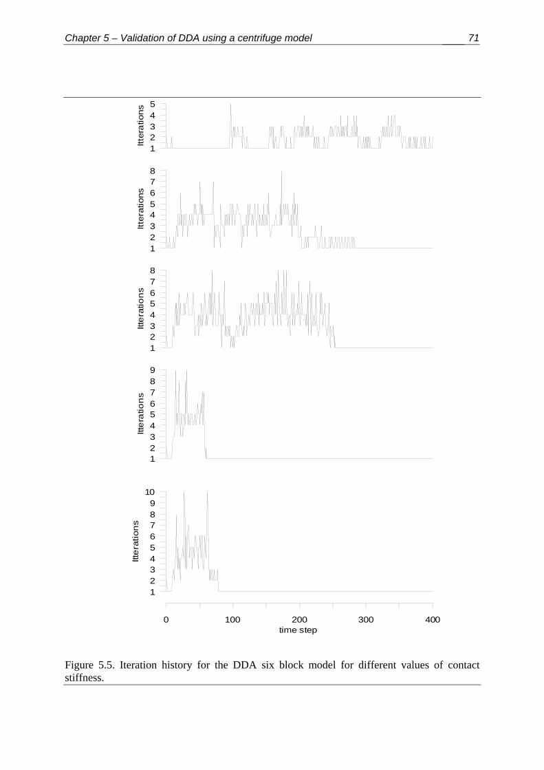
Chapter 5 – Validation of DDA using a centrifuge model 71
12345
Itter
atio
ns
12345678
Itter
atio
ns
12345678
Itte
ratio
ns
123456789
Itte
ratio
ns
0 100 200 300 400time step
123456789
10
Itte
ratio
ns
Figure 5.5. Iteration history for the DDA six block model for different values of contact stiffness.

Chapter 5 – Validation of DDA using a centrifuge model 72
From the discussion above it is concluded that for the given beam geometry and
material properties, a contact stiffness value of g0 = 250 MN/m yields the most accurate
values with respect to displacement, stresses, and convergence of the numeric solution. This
value is used in the DDA simulation of the centrifuge model for a jointed beam.
The DDA model is divided into 12 segments of loading, from 1g to 12 g in 1g
increments, each of 240 time steps, conforming to the convergence criterion described earlier.
DDA loading function of the centrifuge model is depicted in Figure 5.6. The numerical
control parameters and material properties for the DDA model are given in Table 5.1.
5.3.4. Results
The results of DDA are presented in Figure 5.7a and 5.7b that show vertical
displacements and stresses respectively. Clearly, the amount of displacement predicted by
DDA is excessive when compared with the displacements measured in the centrifuge model.
However, the deformation features are similar: most of the displacements are found at the
center of the beam, dying out towards the abutment. Thus, active arching within the
deforming beam can be assumed.
For loading levels of a > 4g, the displacements are very similar, implying stable arching
of the beam. In Figure 5.7b, the horizontal stresses are growing with the g level, suggesting
that arching stresses are building up within the beam. Furthermore, the angle to principal
stresses (θ) within the blocks is growing with g level, as shown in Figure 5.8. For loading
levels of a > 7g the variation of angle θ shows distinct arching: the principal stresses left of
the centerline are rotated in a positive sense (counter-clockwise), whereas the principal
stresses on the right hand side are rotated in a negative sense (clockwise). The magnitude of
the measured and DDA computed stresses are found to be of the same order; the relative
numeric error is 30% to 60% for all loading levels concerned.
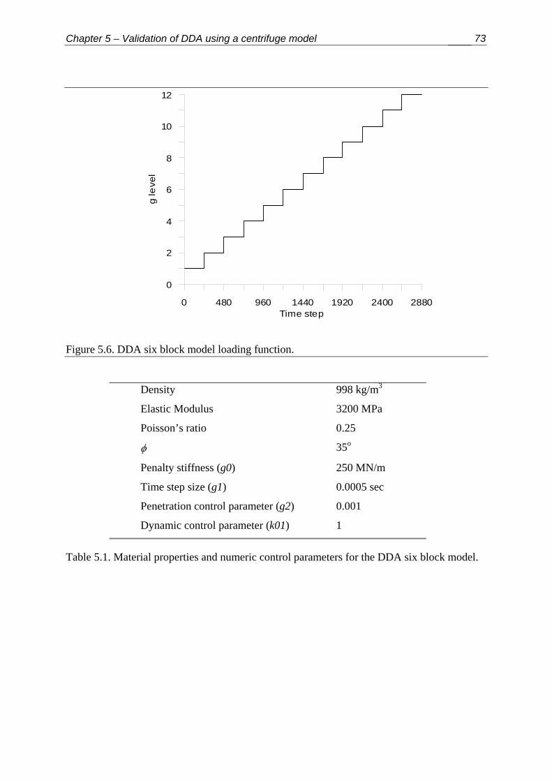
Chapter 5 – Validation of DDA using a centrifuge model 73
0 480 960 1440 1920 2400 2880Time step
0
2
4
6
8
10
12
g le
vel
Figure 5.6. DDA six block model loading function.
Density 998 kg/m3
Elastic Modulus 3200 MPa
Poisson’s ratio 0.25
φ 35o
Penalty stiffness (g0) 250 MN/m
Time step size (g1) 0.0005 sec
Penetration control parameter (g2) 0.001
Dynamic control parameter (k01) 1
Table 5.1. Material properties and numeric control parameters for the DDA six block model.

Chapter 5 – Validation of DDA using a centrifuge model 74
-0.15 -0.1 -0.05 0 0.05 0.1 0.15Distance form center (m)
0.01
0.001
0.0001
1E-005
1E-006
Ve
rtica
l dis
pla
cem
ent
(m)
1g2g3g
4 - 12 g
Centrifuge m
odel1 to 12 g (1 g increm
ents)
DDA
aBlock 1 Block 2 Block 3
0 2 4 6 8 10g level
12
0
40
80
120
160
200
Axi
al F
orce
(N)
DDA centrifuge
Figure 5.7. Comparison between centrifuge model results and DDA solution: a) vertical displacements; b) horizontal stresses.

Chapter 5 – Validation of DDA using a centrifuge model 75
-0.15 -0.1 -0.05 0 0.05 0.1 0.15Distance from centerline (m)
-20
-10
0
10
20
30
θ (d
eg.)
5g
6g
7g8g
9g10g12g
Block 1 Block 2 Block 3
θx
y2
1
Figure 5.8. DDA six block model: angle to principal stresses (θ) within the blocks

Chapter 5 – Validation of DDA using a centrifuge model 76
5.4. Discussion and Conclusions
From the discussion above, it can be concluded that DDA captures the essential features
of the jointed beam deformation, as found in the centrifuge model. Both centrifuge model and
DDA show that an arching mechanism, transfer of vertical load to the abutments, is active
within the beam. Arching precludes displacement of blocks near the abutment, and induces
stability after initial displacement. This is clearly seen at high loading levels, where the
principal stresses are rotated in a symmetric pattern with respect to the centerline, as shown in
Figure 5.8.
However, the exact magnitude of displacements and stresses are not replicated by DDA.
The discrepancies between the centrifuge model and the DDA solution arise from the
following factors:
1. Representation of joints in DDA and centrifuge model.
2. First order displacement approximation in DDA.
These factors are described in section 5.3.3.
The geometric dimensions of the centrifuge model posses additional difficulties. The
individual blocks are very small and tightly packed, and deformations are extremely small,
maximum of 10-5m under low loading levels. The initial perturbation associated with
application of gravity is not fully dissipated through the analysis, and the numeric error
remains high throughout the analysis. Furthermore, since joints exhibit intrinsic plastic
behavior, similarity between the model and full size engineering prototypes is not guaranteed.
When compared with the classic Voussoir mode, l DDA shows a distinct advantage. For
the given geometry, Voussoir model predicts failure at loading level of 1g. The beam buckles
without achieving equilibrium.

Chapter 5 – Validation of DDA using a centrifuge model 77
In DDA the mode of failure, displacements and stresses are governed by the value of
contact stiffness. The magnitude of the contact stiffness is purely numeric, and it is not
associated with normal or shear stiffness of physical interfaces. The choice of the contact
stiffness value should be made according to numeric criteria, such that correct mode of failure
and numeric convergence are achieved.

Chapter 6 – The Tel Beer-Sheva Case Study 76
Chapter 6 – The Tel Beer-Sheva Case Study
6.1. Introduction
Successful validation of numerical models by closed form solutions for simple
problems, or by comparison to small-scale physical models is essential. However, no
analytical solution or laboratory model can duplicate the scale and character of the loading,
boundary and environmental conditions inherent to full-scale problems. Rock masses are
heterogeneous with respect to their mechanical properties, with complex boundary conditions.
Furthermore, in discontinuous rock masses the spatial arrangement of the discontinuities is
complex, and in times only partially attainable. Comparison of numerical predictions to actual
behavior in well-documented case studies can help insure that extrapolation from simple
problems to field scale problems is basically valid.
Case studies used for the validation of a DEM should comply with the following
requirements: (1) a well-defined geometry and boundary conditions; (2) accurately
determined material properties of the continuous rock; (3) accurately determined spatial
distribution of discontinuities and the mechanical properties of discontinuities. The case study
of Tel Beer-Sheva meets these requirements.
The case of Tel Beer-Sheva was previously studied by Benary (1996) and Hatzor and
Benary (1998). Their research showed that: 1) the classic Voussoir model is unconservative for the
given rock mass structure; and 2) the stability of a laminated Voussoir beam is dictated by the
interplay between friction angle along joints and joint spacing.

Chapter 6 – The Tel Beer-Sheva Case Study 77
In this study several issues are explored in greater depth: the mechanical properties of
the rock mass are further explored: transverse isotropy of the continuous rock is defined and
the mechanical properties of the discontinuities are studied using direct shear apparatus.
The numerical part of this study is performed under the guidelines developed in
Chapters 4 and 5. The numerical study emphasizes the kinematics and deformation of both a
single layer and multi-layered roof, with comparison to the classic Voussoir solution.
6.2. Site Description
The ancient site of Tel Beer-Sheva is located approximately 3 km southeast of the
modern city of Beer Sheva. Situated on a hilltop at elevation of 307 m MSL, the site is
bordered by two ephemeral streams (wadi): Wadi Beer-Sheva (south) and Wadi Hebron
(north). The ancient city of Beer-Sheva is dated to the Iron age at 2700 B.P to 3200 B.P. The
ancient water reservoir, dated to 3000 B.P., was used as a water storage facility for times of
drought or siege. A schematic layout of the archeological site and the underlying water
reservoir is presented in Figure 6.1.
The large storage facility beneath the city was fed by seasonal run-offs from Wadi
Hebron, through a tunnel running beneath the city walls. From within the city the access to
the water tank was through a large vertical shaft. The intake capacity of the reservoir,
disregarding support elements, is approximately 250 m3. The walls of the reservoir were
plastered to prevent leakage.
The excavation sequence of the water reservoir is unknown. However, evidence of
failure within the period of excavation, or short time after, is found in the form of a large
support pillars coated with the same plaster. The water reservoir layout is presented in Figure
6.2. The main hall of the reservoir is a rectangle 14 m long and 15 m wide. An elongated
room, 7m long and 3 m wide extruds from the main hall. Two pillars, found at the center of

Chapter 6 – The Tel Beer-Sheva Case Study 78
the main hall, support the roof at areas where failure occurred. The morphology of the failure
zones and their relation to the support pillars are described in section 6.2.2.
6.2.1. Geology
Tel Beer-Sheva is located in an elevated area bordering two major synclinal structures
the Beer-Sheva syncline (south) and the Shefela syncline (north). The water reservoir is
excavated in the sedimentary Gareb formation (Upper Cretaceous), comprised of alteration of
horizontal layers of chalk 0.3m to 0.8m thick, with some thinner (up to 0.1m) layers of marly
chalk of low plasticity and swelling potential (Benary, 1996).
Gareb formation is unconformably overlaid by the polymicitic Ahuzam conglomerate
(Upper Pliocene), locally attaining thickness of up to 6 m, containing cemented, poorly
sorted, angular to rounded pebbles of limestone and chert. Overlying the Ahuzam
conglomerate are Quaternary riverbed deposits, mixed with archeological layers, locally attaining
thickness of 3 m.
6.2.2. Geometrical properties of discontinuities and failure zone morphology
An extensive mapping of joint sets at the site was performed by Benary (1996). The
following section summarizes the main findings by Benary. The joints were mapped both
within the underground water reservoir and a nearby outcrop (within 300 m) exposed by Wadi
Beer-Sheva. Three vertical joint sets where mapped. The geometrical properties of the joint
sets are given in Table 6.1.
Joint sets J1 and J2 are most abundant with mean spacing of 0.2m and 0.25m
respectively. The bedding planes are horizontal with mean spacing of 0.5m. The strike of joint
set J1 is nearly parallel to the axis of the intake tunnel, while J2 is perpendicular to J1 and co-
linear with the reservoir walls. The intersection of the closely spaced joints with the bedding
planes forms a dense network of mostly equidimensional cubic blocks.

Chapter 6 – The Tel Beer-Sheva Case Study 79
Figure 6.1. Schematic drawing of the Tel Beer-Sheva archeological site and the water reservoir. (Source: Hatzor and Benari, 1998).
The excavation of the water reservoir, and consequent stress release, led to spatial
rearrangement of the initial tight packing, where most movement occurred along the pre-
existing joints.
Joint set Dip Strike (o) Mean Spacing (m) Persistence (m)
J1 Sub-vertical 039 – 061 0.2 >10
J2 Sub-vertical 124 – 127 0.25 Bounded by J1*
J3 Vertical 107 – 112 0.6 >15
Bedding Horizontal 0.5 Infinite
Table 6.1. Principal joint sets in the Gareb chalk at Tel Beer-Sheva site, from Benary (1996).

Chapter 6 – The Tel Beer-Sheva Case Study 80
The roof of the water reservoir collapsed into a shape of a three dimensional dome.
Three distinct levels where mapped by Benary (1996):
• Original excavation level at absolute level of 286 m – Zone 1.
• Intermediate failure level at absolute level of 287 m – Zone 2.
• Upper failure level at absolute level of 289 m – Zone 3.
All zones are developed along natural bedding planes. The transition between the
different levels ranges from vertical to step like, running along block boundaries, defined by
the intersections of joints and bedding planes. Longitudal and transverse cross sections are
presented in Figure 6.3a,b respectively.
The western pillar supports the roof at Zone 3. The lateral extent of the pillar is
unknown due to plaster coating. However, given the fact that the pillar supports the
uppermost failure zone, the minimum extent is within the boundaries of Zone 3. Furthermore,
lining extends beyond the boundaries of Zone 3 into Zone 2, where the host rock s is exposed.
The exposure of rock mass at the extreme end of the western pillar is found to be in line with
the external wall of the access shaft. Based on these observations the minimum extent of the
western pillar is drawn (dashed line at Figure 6.2). The eastern pillar supports Zone 2, and
does not attain Zone 3. Again, the lateral extent is not clear. However, based on similar
considerations the extent of the pillar is drawn. Plaster coating of the reservoir walls is
confined to Zone 1 level, and original chisel marks are found only at Zone 1.
Based on all previously described observations the assumed minimum active span of
the opening at the time of failure was 8 meters, conforming with Zone 3. The assumed
maximum active span, drawn at Figure 6.2, was 10 meters conforming to Zone 2.

Chapter 6 – The Tel Beer-Sheva Case Study 81
6.3. Mechanical Properties of Intact Rock
6.3.1. Experimental procedure
Intact rock samples were tested using hydraulic, closed-loop, servo-controlled, triaxial
load frame (TerraTek system model FX-S-33090) with stiffness of 5×10⁹ N/m. Axial and
radial strains were recorded using four arm axial and radial strain cantilever sets with 10%
and 7% strain range respectively, both with 1% linearity full scale. Total axial load capacity
in compression was 1400 kN, but the applied axial load was limited by the load cell capacity.
In this research we used a 222 kN load cell, with over range capacity of 100%, and 0.5%
linearity full scale, for better resolution of low loads. Axial stroke capacity was 113.78mm.
All tests were performed under a constant strain rate of 10-5 s-1; and complete stress-strain
curves were obtained.
Solid cylinders were prepared according to ASTM standards (D4543-85 and D2216-
92) regarding end roughness (0.01 mm) and perpendicularity (0.005 radians). Uniaxial tests
were performed according to ASTM standard D3148-93. The cylinder axes were oriented
parallel to bedding planes (the angle between the normal to bedding planes and maximum
principal stress 1σ is ). 90=β
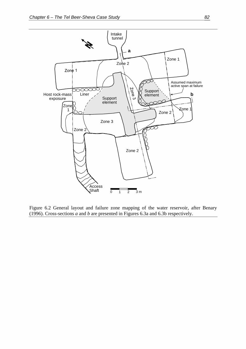
Chapter 6 – The Tel Beer-Sheva Case Study 82
Zone 1
Zone 1Zone
1
Zone 2
Zone 2
Zone 2
Zone 2
Zone 3
Liner
0 1 2 3 m
Assumed maximumactive span at failure
Supportelement
SupportelementHost rock-mass
exposure
Intake tunnel
AccessShaft
b
a
Figure 6.2 General layout and failure zone mapping of the water reservoir, after Benary (1996). Cross-sections a and b are presented in Figures 6.3a and 6.3b respectively.

Chapter 6 – The Tel Beer-Sheva Case Study 83
-2 0 2 4 6 8 10 12 14 16 18 20 22
280
282
284
286
288
290
292
294
Zone 1
Zone 2
Zone 3
Chalk
Conglomerate
-1 0 1 2 3 4 5 6 7 8
285
286
287
288
289
Zone 1
Zone 2
Zone 3
a
b
Figure 6.3. Cross-sections of the water reservoir: a) longitudal cross-section; b) transverse cross-section (Source: Benari, 1996).

Chapter 6 – The Tel Beer-Sheva Case Study 84
The tested samples were drilled from two blocks extracted from two overlaying beds
in a natural riverbed outcrop below the archeological site of Tel Beer-Sheva, where the level
of exposure is approximately at the level of the water reservoir.
Benary (1996) performed both uniaxial and triaxial tests oriented normally to bedding
planes (i.e. ), on samples taken from two vertical cores which penetrated the reservoir
beds.
0=β
6.3.2. Test results
Four samples were tested here under uniaxial compression, the mechanical properties
of which are summarised in Table 6.2. Two representative stress-strain curves for uniaxial
compression at and are shown in Figure 6.4. The variation in the mechanical
properties between samples TBS-1 and TBS-2 can be attributed to local variations as
described in the previous section.
90=β 0=β
Gareb chalks exhibit pronounced anisotropy both in strength and in elasticity. The
unixial compressive strength ratio (090 == ββ
UCSUCS ) varies from 3 to 5, and the elastic
modulus ratio ( 090 =β=βEE ) is varies from 3 to 4. Transverse isotropy parallel to bedding
planes is assumed: in three tests the radial strains ( 21 RR εε ⊥ and aligned parallel to beddings)
exhibit essentially identical behavior, with inter-strain linear coefficient ranging from 0.98 to
1.1.
6.3.3. Estimation of the in-situ stresses
Based on these findings the in-situ stresses can be estimated. The vertical stress is
assumed gravitational, given by gzv ρσ = where z is depth. The ratio of horizontal to vertical
stresses vhk σσ= , may be estimated using the elasto-static thermal model of Sheorey (1994):

Chapter 6 – The Tel Beer-Sheva Case Study 85
⎟⎠⎞
⎜⎝⎛ ++=
zEk h
1001.0725.0 (6.1)
where (m) is depth below surface and Ez h (in GPa) is the average deformation
modulus measured in the horizontal direction. This direction of measurement is important
particularly in layered sedimentary rocks, in which the deformation modulus may be
significantly different in different directions. For the case of Tel Beer-Sheva GPaEh 485.7=
A direct measurement of the in-situ horizontal stress was not performed in this
research. However, hydraulic fracturing measurements by Polishook (1995), at a site located
about 15 km southwest from Tel Beer-Sheva at depths of 52-70 meters show good agreement
with Sheorey’s model (refer to Figure 6.5). The measurements where performed on younger
Eocene strata (Adulam formation), composed mainly of horizontally layered thick chalk,
within the Beer Sheva syncline. Good agreement between the measured and calculated values
supports the applicability of the model, and precludes significant contribution from
overlooked tectonic stresses.

Chapter 6 – The Tel Beer-Sheva Case Study 86
-2 -1.5 -1 -0.5 0 0.5 1 1.5 2Strain (%)
0
5
10
15
20
25
30
35
Axi
al S
tress
(MP
a)
β = 90ο
β = 0ο
AxialRadial
Figure 6.4 Complete stress-strain curves for the Gareb chalk at uniaxial compression parallel (β=90ο, this study) and normal to bedding (β=0ο, Benari, 1996).
Sample β (ο) ρ (kg/m3) n (%) E (GPa) ν (%) UCS (MPa)
TBS-1a 90 1930 28 8.34 0.172 34.12
TBS-1b 90 1960 27 8.16 0.160 29.35
TBS-2a 90 1880 30 6.94 0.164 25.08
TBS-2b 90 1850 31 6.50 0.190 21.78
Benary (1996) 0 1910* 29* 1.9 0.05 6.6
* average value.
Table 6.2. Mechanical properties of the Gareb chalk at Tel Beer-Sheva. ρ is density, n is porosity (calculated for G.S. = 2.7), ν is Poisson’s ratio, E is elastic modulus, and UCS is unconfined compressive strength.
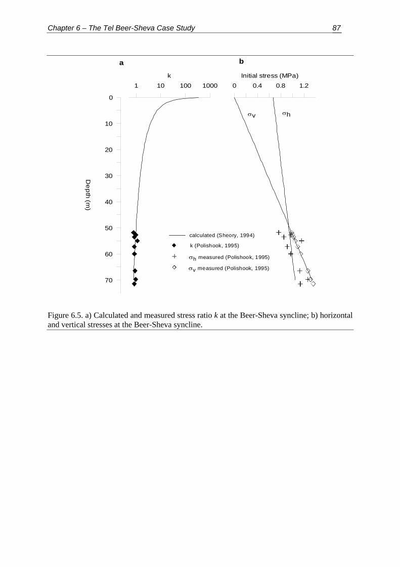
Chapter 6 – The Tel Beer-Sheva Case Study 87
0
10
20
30
40
50
60
70
De
pth
(m)
1 10 100 1000k
0 0.4 0.8 1.2Initial stress (MPa)
σhσv
calculated (Sheory, 1994)
σh measured (Polishook, 1995)
σv measured (Polishook, 1995)
k (Polishook, 1995)
a b
Figure 6.5. a) Calculated and measured stress ratio k at the Beer-Sheva syncline; b) horizontal and vertical stresses at the Beer-Sheva syncline.
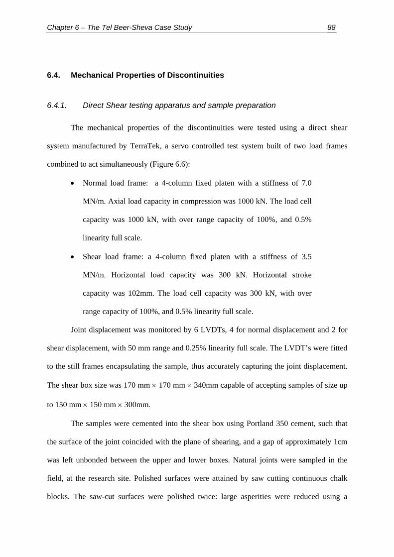
Chapter 6 – The Tel Beer-Sheva Case Study 88
6.4. Mechanical Properties of Discontinuities
6.4.1. Direct Shear testing apparatus and sample preparation
The mechanical properties of the discontinuities were tested using a direct shear
system manufactured by TerraTek, a servo controlled test system built of two load frames
combined to act simultaneously (Figure 6.6):
• Normal load frame: a 4-column fixed platen with a stiffness of 7.0
MN/m. Axial load capacity in compression was 1000 kN. The load cell
capacity was 1000 kN, with over range capacity of 100%, and 0.5%
linearity full scale.
• Shear load frame: a 4-column fixed platen with a stiffness of 3.5
MN/m. Horizontal load capacity was 300 kN. Horizontal stroke
capacity was 102mm. The load cell capacity was 300 kN, with over
range capacity of 100%, and 0.5% linearity full scale.
Joint displacement was monitored by 6 LVDTs, 4 for normal displacement and 2 for
shear displacement, with 50 mm range and 0.25% linearity full scale. The LVDT’s were fitted
to the still frames encapsulating the sample, thus accurately capturing the joint displacement.
The shear box size was 170 mm × 170 mm × 340mm capable of accepting samples of size up
to 150 mm × 150 mm × 300mm.
The samples were cemented into the shear box using Portland 350 cement, such that
the surface of the joint coincided with the plane of shearing, and a gap of approximately 1cm
was left unbonded between the upper and lower boxes. Natural joints were sampled in the
field, at the research site. Polished surfaces were attained by saw cutting continuous chalk
blocks. The saw-cut surfaces were polished twice: large asperities were reduced using a
Chapter 6 – The Tel Beer-Sheva Case Study 89
Silicon Carbide grit 120 polishing powde;, final leveling was attained using Silicon Carbide
grit 300 polishing powder.
6.4.2. Direct shear tests of natural joint
Two-segment tests were performed on TBS-1, both performed under constant
displacement rate (shear rate of 0.00127 mm/sec). The joint was tested as sampled without
any additional treatment. Normal load was increased between the segments to obtain a failure
envelope. Test TBS-1 was performed under normal loads of 0.7 MPa; 1.7 MPa; 3.7 MPa. Test
TBS-1A was performed under normal loads of 2.95 MPa; 4.95 MPa and 6.95 MPa. The
results are presented in Figure 6.7a, and the variation of resulting friction angle as a function
of normal stress is given in Figure 6.7b. Peak friction angle under the specified loading
condition was φ = 47o (at σn = 700 kPa, not shown in Figure 6.7a), the friction angle was
reduced during the test down to a value of φ = 24o. Degradation of the friction angle as a
function of increasing normal stress represents the degradation of the asperities along the joint
surface. Thus, the peak friction angle is φp = 47o and the residual friction angle is φr = 24o, the
maximum roughness angle is i = φp − φr = 23o.
6.4.3. Shear rate effect – polished interface
In order to attain better understanding of artifacts associated with shear rate a single
polished surface was tested under varying rate conditions. Sample TBS-2 was subjected to
three cycles of shearing under different shear rates: 0.0033 mm/sec, 0.0127 mm/sec and
0.0254 mm/sec. The normal stress was set constant for all three tests at 3150 kPa. Results of
the test are given in Figure 6.8. Friction angle for the three cycles is practically the same, φ =
29o for forward shear and φ = 25o for backward shear. The shear stiffness, given in Figure
Chapter 6 – The Tel Beer-Sheva Case Study 90
6.8b, shows a pronounced strain rate effect. The strain rate and shear stiffness are inversely
proportional: with lower shear rate resulting in higher stiffness.
The nature of the shearing process is changed as well during the increase of shear rate.
For low shear rate, 0.0033 mm/sec, shearing is clearly of stick slip type with shear stress
amplitude variation of approximately ±100 kPa. With increased shear rate the amplitude of
the stick slip oscillations is reduced to approximately ±30 kPa. Further increase in shear rate
reduced the oscillations to values lower than ±10 kPa. It is unclear whether this is a shear rate
effect, or roughness degradation due to cyclic shearing. Constant value of friction angle
during the consecutive shearing cycles implies that roughness is negligible.
6.4.4. Direct shear tests of a polished interface
Sample TBS-4, a polished surface, was tested under various normal loading
conditions. Normal stress levels were: 500 kPa, 1000 kPa, 1500 kPa, and 2000 kPa. The shear
rate was set constant at 0.0254 mm/sec. Shear displacement – shear stress curves for sample
TBS – 4 are given in Figure 6.9a. The shear stiffness values showed proportional increase
with the increase in normal stress (Fig 6.9b), as expected. Friction angles during shearing
cycles show pronounced anisotropy. During forward shear the friction angles reduced from φ
= 47o at σn = 500 kPa to φ = 38o at σn = 2000 kPa (Fig 6.9c). For backward shear the friction
angles rose from φ = 30o at σn = 500 kPa to φ = 35o at σn = 2000 kPa.
Dilatancy data and visual examination of the sample revealed that friction anisotropy
is related to accumulation of crushed material (bulge) along the shear interface during the first
cycle. The geometry of the bulge was such that during forward shear the relative motion
between the mating surfaces led to vertical contraction, while backward shear led to vertical
dilation. The bulge was mechanically reduced during the consecutive cycles of shear. The
difference between the forward – backward friction angles decreased, from 14o at σn = 500

Chapter 6 – The Tel Beer-Sheva Case Study 91
kPa to 2o at σn = 2000 kPa. Friction angle value converged to φ = 35o at σn = 2000 kPa.
Friction angle for a polished chalk surface as measured at sample TBS – 2 is φ = 25o - 29o.
The differences between these two values represent the residual geometry and shear strength
of the bulge. Such a phenomenon can occur in natural environments when shear initiates
along discontinuities in weak rock. Crushing of intact rock material in the vicinity of
discontinuity can cause an accumulation of rock material along the shear surface, thus
significantly contributing to shear resistance along the sliding plane.
Direct shear tests for this research were performed under constant normal stress
(CNS). This configuration is less suitable for underground applications where shear sliding of
blocks is usually constrained between joints, and therefore best represented by constant
normal position (CNP) tests. The friction angle attained from CNS tests is usually lower than
one attained from CNP tests. However, the deformation of the jointed beams is such that both
position and normal stresses are changed during deflection. Therefore, neither CNP nor CNS
tests are truthful replica of the shear processes active in jointed beam deformation.

Chapter 6 – The Tel Beer-Sheva Case Study 92
Figure 6.6. Direct shear system at the Rock Mechanics Laboratory of the Negev: a) general view; b) assembled shear box and displacement detectors (LVDT’s).
Chapter 6 – The Tel Beer-Sheva Case Study 93
0 1 2 3 4 5
Shear Displacement (mm)
6
-1000
0
1000
2000
3000
4000S
hear
Stre
ss (k
Pa)
0 2000 4000 6000 8000Normal Stress (kPa)
0
10
20
30
40
50
φ (d
eg.)
σn = 1700 kPa
3700 kPa2950 kPa
4950 kPa
6950 kPa
ln(φ) = -0.313 * ln(σn) + 5.836
R-squared = 0.896
a
b
Figure 6.7. Direct shear results of a natural joint in Gareb formation, sample TBS-1: a) shear displacement vs. shear stress; b) friction angle vs. normal stress.

Chapter 6 – The Tel Beer-Sheva Case Study 94
-1 -0.8 -0.6 -0.4 -0.2 0 0.2 0.4 0.6 0.8 1
Shear Displacement (mm) -2000
-1500
-1000
-500
0
500
1000
1500
2000
She
ar S
tress
(kP
a)
dU/dt = 0.0033 mm/sec
dU/dt = 0.0127 mm/sec
dU/dt = 0.0254 mm/sec
0 0.005 0.01 0.015 0.02 0.025 0.03Shear rate (mm/sec)
6000
8000
10000
12000
Ks
(kP
a/m
m)
a
b
forward shear
backward shear
Figure 6.8. Direct shear results for polished surface in Gareb chalk, sample TBS – 2: a) shear stress – shear displacement curves; b) shear stiffness ks as a function of shear rate.
dU/dt (mm/sec) ksf (kPa/mm) ksb (kPa/mm)
0.0033 11,700 9500
0.0127 9500 7700
0.0254 8830 6550
Table 6.3. Shear stiffness at different shear rate values for sample TBS-2. dU/dt is shear rate, ksf and ksb are shear stiffness for forward shear and backward shear respectively.

Chapter 6 – The Tel Beer-Sheva Case Study 95
-2.5 -2 -1.5 -1 -0.5 0 0.5 1 1.5 2 2.5
Shear Displacement (mm)-1600
-1200
-800
-400
0
400
800
1200Sh
ear S
tress
(kP
1600a)
1000 kPa
500 kPa
1500 kPa
Normal Stress = 2000 kPa
0 500 1000 1500 2000Normal Stress (kPa)
0
2000
4000
6000
8000
Ks
(kP
a/m
m)
0 500 1000 1500 2000Normal Stress (kPa)
0
10
20
30
40
50
φ (d
eg.)
forward shear
backward shear
b c
friction difference
a
Figure 6.9. Direct shear results for a polished surface, sample TBS-4: a) shear displacement vs. shear stress; b) shear stiffness (ks) vs. normal stress; c) friction angle (φ) vs. normal stress

Chapter 6 – The Tel Beer-Sheva Case Study 96
-4 -2 0 2 4∆u (mm)
-0.4
-0.2
0
0.2
0.4
∆v (m
m)
σn = 500 kPa
-4 -2 0 2 4∆u (mm)
-0.4
-0.2
0
0.2
0.4
∆v (m
m)
-4 -2 0 2 4∆u (mm)
-0.4
-0.2
0
0.2
0.4
∆v (m
m)
-4 -2 0 2 4∆u (mm)
-0.4
-0.2
0
0.2
0.4∆v
(mm
)
σn = 1000 kPa
σn = 1500 kPa σn = 2000 kPa
Figure 6.10. Sample TBS-4: normal displacement (∆v) vs. shear displacement (∆u) at different levels of normal stress.

Chapter 6 – The Tel Beer-Sheva Case Study 97
6.5. Stability Analysis Using Classical Voussoir Model
Stability analysis of the Tel Beer-Sheva water reservoir was performed using the
iterative procedure (Appendix) introduced by Brady and Brown (1985), and corrected by
Diederichs and Kaiser (1999). The mechanical properties of the rock mass in-situ were used
in the analysis (Table 6.4.). Since the rock mass was found to be transversely isotropic the
values of E, ν, and UCS chosen for the analysis were the values measured in the direction
parallel to bedding, which for the case of a roof in horizontally oriented layers is horizontal.
Three modes of failure were considered: (1) lateral compressive failure at mid-span and
abutments; (2) shear along abutments; and (3) snap through (buckling).
Density 1900 kg/m3
Elastic Modulus 7840 MPa
Poisson’s ratio 0.17
UCS 27.6 MPa
Friction angle along joints 47o
Table 6.4. Representetive material properties of the Gareb Chalk.
The factor of safety against failure in compression and in shear was calculated for a
wide range of beam geometries. The beam span (S) was varied from 5m to 16m, thus
accounting for most possible geometries at time of failure. The beam thickness (t) was varied
from 0.25m to 5m, from a single bed to the total thickness of the chalk layers, respectively.
An equation for the Factor of Safety (F.S.) against failure in compression is given in
equation A9 of the Appendix, and the results as calculated for this study are plotted in Figure
6.11a. For beam thickness lower than 0.5m and span greater than 10m the failure is by snap
through, indicated by a non-converging solution. The factor of safety against failure in

Chapter 6 – The Tel Beer-Sheva Case Study 98
compression for all other geometries is greater than 3, increasing for thicker beams due to
larger moment arm (Z) and lower axial stress (fc).
An equation for the Factor of Safety (F.S.) against shear along abutments is given in
equation A10 of the Appendix, and the results as calculated for this study are plotted in Figure
6.11b, where the beam span is normalized to beam thickness. Assuming that the peak friction
angle along joints is φ = 47ο, as found by direct shear tests, and assuming that the active span
at time of failure was 8m, the factor of safety against shear ranges from to
for beam thickness ranging from 0.5m to 5m respectively. Assuming that the
active span at time of failure was 12m, the factor of safety against shear ranges from
to for beam thickness ranging from 0.5m to 5m, respectively. Beams
of low S/t ratio are prone to shear failure since the required moment arm (Z) for equilibrium
increases with decreasing aspect ratio.
3.8.. =SF
83.0.. =SF
4.12.. =SF 24.1.. =SF
Assuming a roof span of 8m and layer thickness of 5m the failure of the ancient water
reservoir at Tel Beer Sheva can be explained using the Brady and Brown procedure.
However, this is not the case: the thickness of Zone 3 is 1m to 2m which is the maximum
active thickness of the failed layer. Given a thickness of 2m the factor of safety against shear
failure is , for beam thickness of 1m the factor of safety is even higher than . 2.. =SF 4.. >SF
For active span greater than 8m the factor of safety rises above 1 for all thickness
values considered. Moreover, for beam with r = S/t > 4, the required friction angle for
stability is φ > 47ο. Therefore, under the given geometrical constraints and material properties
the roof would not fail according to the Brady and Brown procedure.
From the described above it is concluded that classic Voussoir procedure is
unconservative, predicting required friction angles for roof stability lower than the available
friction angle along joints. The unconservative nature of the analysis can be attributed to the
following factors:
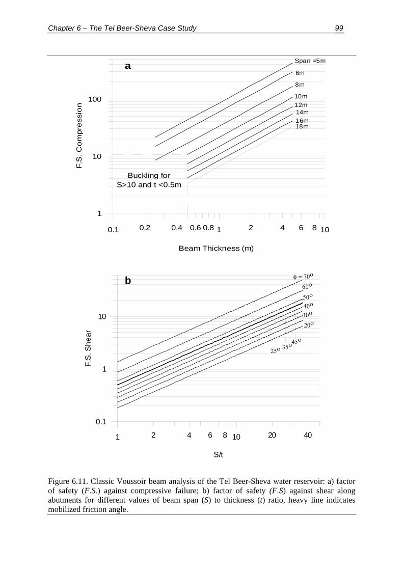
Chapter 6 – The Tel Beer-Sheva Case Study 99
0.1 1 100.2 0.4 0.6 0.8 2 4 6 8
Beam Thickness (m)
1
10
100
F.S
. Co
mpr
ess
ion
Span =5m
6m
8m
10m12m14m16m18m
Buckling forS>10 and t <0.5m
a
1 102 4 6 8 20 40
S/t
0.1
1
10
F.S
. She
ar
20ο
25ο
30ο
35ο
40ο
45ο
50ο60ο
φ = 70οb
Figure 6.11. Classic Voussoir beam analysis of the Tel Beer-Sheva water reservoir: a) factor of safety (F.S.) against compressive failure; b) factor of safety (F.S) against shear along abutments for different values of beam span (S) to thickness (t) ratio, heavy line indicates mobilized friction angle.
Chapter 6 – The Tel Beer-Sheva Case Study 100
1) Large number of discontinuities - the rotational freedom required for stable arching
in a multi-fractured beam is larger than the one required for a three-hinged beam. In a closed
domain, such as the densely fractured and tightly packed rock mass of Tel Beer-Sheva, this
requirement is compromised. Consequently, the vertical reaction at the abutments is not fully
developed. Thus, under gravitational loading the beam will shear along the abutments.
Therefore, the friction angle required for equilibrium according to the Voussoir analysis will
be significantly lower than the one required for a multi fractured beam.
2.) Partial inter-bed separation - Voussoir analysis assumes that the rock mass has
parted along smooth breaks forming a series of beams, thus assuring that no gravitational load
is transferred to the lower members of the beam stack. In the case of Tel Beer-Sheva this
assumption is not satisfied; the failed rock mass consisted of up to 4 individual beds
(assuming total thickness of 2m). Thus, a vertical load transfer between beams should be
considered.
When the roof is excavated in a densely fractured rock mass the classic Voussoir
solution is shown to be inadequate. The large number of individual blocks, and their
interactions, impedes on the analytical solution. It is concluded, therefore that for a realsitic
solution a numerical scheme must be employed. In the next section a back analysis of the
failure at Tel Beer-Sheva using DDA is presented. The focus of the analysis is on the
kinematics of a multi-block structure. The deformation of the roof as a function of joint
mechanical and geometrical properties is studied, and some limitations of DDA are explored.

Chapter 6 – The Tel Beer-Sheva Case Study 101
6.6. Numerical Analysis Using DDA
6.6.1. Numerical problems associated with multi-block systems
The transition from simple problems with a limited number of blocks to full-scale
problems where the number of blocks is large (hundreds to thousands) introduces numerical
problems associated with the large number of contacts involved. Most of the difficulties are
associated with the no penetration/no tension contact constraint between blocks, which is the
criterion controlling the convergence of the solution in each time step. In the numerical
implementation of this criterion a small penetration is used. Proper choice of the penetration
control parameter (g2) assures that: there are no unnecessary contacts (where g2 is to large) or
penetrations (where g2 is to small).
In Chapter 4 it has been shown that: 1) the numeric control parameters are interrelated;
and 2) the accuracy of the solution is governed by the conditioning of the global stiffness
matrix. Best accuracy is achieved for optimized time step size (g1) and contact stiffness (g0).
In DDA the contacts between blocks are represented by elastic springs, rather than by a
constitutive joint model. Therefore, the stiffness value should be chosen such that it complies
with numeric convergence rather than with natural joint stiffness values.
The effect of g1and g0 parameters on the convergence rate of DDA solution for a
multi-block system was studied for three cases: 1) 67 blocks; 2) 98 blocks; and 3) 168 blocks.
All configurations consisted of a stack of jointed beams, similar to the configuration presented
in Figure 6.14b. Each case was modeled for four different g1, g2 couples, which for
simplicity where assumed equal: 1) g1=g2=0.01; 2) g1=g2=0.005; 3) g1=g2=0.001; and 4)
g1=g2=0.0005. The penalty stiffness for each g1, g2 couple was varied in incriments from
50·MN/m to 100,000 MN/m. All simulations were performed for k01 = 1, the number of time
Chapter 6 – The Tel Beer-Sheva Case Study 102
steps was set such that the total time of each simulation was 0.25 sec. Material properties of
the blocks were set to E = 7.48 GPa, ν = 0.17, and ρ = 1.9·103 kg/m3 (Gareb chalk). Friction
angle along joints was set to φ = 45o (µ = tanφ = 1). The results of the analysis are presented
in Figure 6.13, which is a series of plots showing the average number of iterations for a time
step iav = i/n (where i is the total number of iterations and n is the total number of time steps)
as a function of penalty stiffness for different values of g1, g2.
For g1 = g2 = 0.01 the average number of iterations per time step increases with g0,
in a nearly linear fashion. For the configuration of 67 blocks the solution diverges when g0 >
100 MN/m, whereas for the configurations of 98 and 168 blocks the solution converges up to
g0 = 10,000 MN/m, where iav values increase up to 24 iterations per time step.
For g1 = g2 = 0.005 the solution converges for all studied configurations, with iav
ranging from 2 to 16 for all values of g0. Setting g1 = g2 = 0.001 improves the convergence
rate of the solution: for 50 MN/m < g0 < 1000 MN/m the convergence rate is nearly constant
at iav = 1.8 for all studied configurations. Increased g0 degrades the convergence rate, as iav =
6.4 at g0 = 50,000 MN/m. For g1 = g2 = 0.0005 the solution rapidly converges for 50 MN/m
< g0 < 5000 MN/m for all studied configurations, with iav ≤ 1.5. Setting g0 > 5000 MN/m
degrades the convergence rate, up to values of iav = 3.5.
From the discussion above it is clear that for multi block configurations the DDA
solution converges independently of penalty stiffness value (g0), provided that the time step
size (g1) and penetration control parameter (g2) are sufficiently small. In Chapter 4 it was
shown that the accuracy of the numeric solution is improved for high values of penalty
stiffness. Based on these observations it can be concluded that the numeric control parameters
for multi block analysis should be chosen such that solution accuracy is not compromised by
the convergence rate, and that the failure mode is correct.

Chapter 6 – The Tel Beer-Sheva Case Study 103
10 100 1000 10000g0 ( 106 N)
0
4
8
12
16
20
24i a
v =
i/ng1 = g2 = 0.01
10 100 1000 10000g0 (106 N)
0
4
8
12
16 g1 = g2 = 0.005
10 100 1000 10000 100000g0 ( 106 N)
0
2
4
6
8
i av
= i/n
g1 = g2 = 0.001
10 100 1000 10000 100000g0 ( 106 N)
1
2
3
4 g1 = g2 = 0.0005
67 blocks98 blocks168 blocks
Figure 6.13. DDA multi block model: average number of iterations per time step (iav = i/n) as a function of penalty stiffness (g0) for different values of time step size (g1) and penetration control parameter (g2).

Chapter 6 – The Tel Beer-Sheva Case Study 104
6.6.2. DDA analysis of the Tel Beer-Sheva water reservoir – numerical setup
DDA analysis of the Tel Beer-Sheva ancient water reservoir was performed for two
geometric configurations:
1. A single layer of thickness t = 0.5 m, representing the immediate roof of
the excavation, Figure 6.14a.
2. A 5m stack of horizontal beams, each of thickness t = 0.5 m, conforming
with the actual roof thickness, Figure 6.14b.
The active span of both configurations was set to S = 8m. While configuration 1 is
compatible with the Voussoir model, configuration 2 is a realistic model of the roof of the
water reservoir. Two fixed blocks, each containing three fixed points, represent the
abutments.
The effect of joint friction was studied for a constant joint spacing of Sj = 0.25m (in
accordance with the average spacing of J1 and J2 observed at the site) while the friction along
joints (φav) was varied from φav = 20o to φav = 80o. The effect of friction angle was studied for
φav = 47o (peak friction angle from direct shear tests) while joint spacing was changed from Sj
= 0.25m to Sj = 4m. For configuration 1 the displacements where measured at the lower fiber
of the beam at selected points in intervals of 0.5m. For configuration 2 the displacements
where measured at five locations as shown in Figure 6.14b: 1) m1- mid-span of immediate
roof; 2) m2 - mid-span at m1+2.5m; 3) m3 - mid span at m1+5m; 4) m4 - left abutment at
m1+2.5m; 5) m5 - right abutment at m1+2.5m.
Material properties of the Gareb chalk and numeric control parameters of DDA
analysis are given in Table 6.5. The joints are modeled as no-tension, no-cohesion interfaces,
namely shear resistance along joints is purely frictional, in compliance with field findings.

Chapter 6 – The Tel Beer-Sheva Case Study 105
Density 1900 kg/m3
Elastic Modulus 7840 MPa
Poisson’s ratio 0.17
Penalty stiffness (g0) 1000 MN/m
Time step size (g1) 0.00025 sec
Penetration control parameter (g2) 0.00025
Dynamic control parameter (k01) 1
Table 6.5. Material properties and numeric control parameters for the DDA model of the Tel Beer-Sheva water reservoir.
In the field, the chalk layers are overlain unconformably with a 5m thick conglomerate
layer; the unconformity plane is considered open and discontinuous. The conglomerate layer
in the field is continuous without apparent cracks or joints.
The first order displacement approximation in DDA results in constant stress/strain
elements. Therefore, because the conglomertae layer consists of a single block, its
deformation cannot be modeled properly with DDA. Consequently the vertical deflection of
the layer and vertical load on the chalk cannot be evaluated accurately. Since the
conglomerate layer is continuous, however, the mid-span deflection can be assessed by
analogy to an elastic, simply supported beam (Obert and Duval, 1967). The mechanical
properties of the conglomerate layer are unknown since the material is highly heterogeneous;
assuming a low stiffness of E = 100 MPa the deflection at mid-span would be δ = 0.00094m,
for E = 1000 MPa the deflection at mid-span would be δ = 0.000094m. These defelection are
quite small and , therefore, it is assumed that load transfer between the conglomerate and the
chalk is negligible; hence, the conglomerate layer is not modeled here.

Chapter 6 – The Tel Beer-Sheva Case Study 106
Sj
S
t
m3
m2
m1
m4 m5
Fixedpoint
a
b
Figure 6.14. Geometry of DDA model of the Tel Beer-Sheva water reservoir: a) single layer model; b) multi-layered model.

Chapter 6 – The Tel Beer-Sheva Case Study 107
6.6.3. DDA analysis of the single layer configuration
The results of DDA analysis for the single layer configuration are presented in Figure
6.15a, which is a plot of mid-span deflection (δ) after 0.25sec versus friction angle (φ) and
joint spacing (Sj). Figures 6.15b,c are time histories of mid-span deflection for different
values of friction angle and joint spacing respectively.
Given joint spacing of Sj = 0.25m the beam deflects progressively and eventually fails
for friction angles of φav < 78o. For friction angles of φav ≥ 78o the beam attains stable
equilibrium after small initial deflection. Figures 6.16a,b,c show the displacements, u, v, and
rotation ω respectively, of the lower fiber after 0.25sec for selected values of friction angle: a)
30o; b) 45o; c) 75o; d) 80o. DDA graphic outputs of the final deformed positions of the blocks
for these selected values of friction are presented in Figure 6.17.
At low values of φav = 30o and φav = 45o most of the deformation is achieved through
deferential inter-block shear, which attains maximum at the mid-span and minimum at the
abutments. The rotation of the blocks is mostly uniform and symmetric, up to ±0.1 radians,
where at the left hand side of the beam the blocks rotate clockwise and vice versa. Similar
beam deflection profile was attained by Evans (1941) while experimenting with brick beams.
The deformation characteristics are changed when the friction angle along joints rises, e.g. φav
= 75o and φav = 80o, inter-block shear is reduced while the rotation at the beam ends rises to
±0.3 radians.
From the rotation data it is evident that at low values of friction angle the moment arm
of the lateral couple is not developed effectively and beam deformation occurs mainly due to
inter-block shear, which consequently leads to failure. Where the available shear resistance
along joints is sufficiently high to preclude excessive vertical displacements, block rotation
Chapter 6 – The Tel Beer-Sheva Case Study 108
and build-up of lateral thrust equilibrate the overturning moment of the vertical couple, and
the beam reaches equilibrium position.
Increasing the block aspect ratio (rb = Sj/t) of the individual blocks by setting Sj = 0. 5m
(rb = 1), and assuming peak friction angle of φav = 47o (peak friction angle from direct shear
tests), results in mid-span deflection of δ = 0.08 m (after 0.25 sec), compared with δ = 0.22 m
for Sj = 0. 25m. However, the beam does not attain equilibrium, and eventually fails.
Examination of the deformation time histories for beams of different aspect ratio (Figure
6.15c) reveals that equilibrium is marked by the oscillatory nature of the solution (this effect
was described in section 6.6.1), as opposed to gradually increasing deflection of failing
beams. Equilibrium is met when rb ≥ 2.5 (Sj ≥ 1.25) and δ ≤ 0.025 m. The style of deformation
is similar: for unstable geometry the beam fails by inter-block shear, with relatively small
rotations, while for stable geometries stability is achieved through effective rotation.
From the described above it is evident that a single beam of span S = 8m, thickness t =
0.5m, block aspect ratio rb =Sj/t= 0.5, and friction angle along joints of φav = 47o is not stable.
Stability is assured for φav ≥ 78o. According to classical Voussoir solution for beam of span S
= 8m, thickness t = 0.5m (block aspect ratio rb = 8) stability is assured for φav > 20o, with
expected deflection of δ = 0.002 m. DDA analysis predicts similar deflection for block aspect
ratio of rb = 4.
The underlying assumption of immediate roof (single layer) analysis is that vertical
load from overlaying layers is transmitted laterally to the abutments, rather than vertically as
transverse loads to the lower layers. This condition is not satisfied within the layers overlying
the water reservoir, namely the failure zone is up to 2.5m thick. Given average bed thickness
of t = 0.5m the failure zone contained 5 individual layers. The stability of a multi-layered and
jointed structure, the laminated Voussoir beam (a term introduced by Hatzor and Benary,
1998), is explored in the following section.

Chapter 6 – The Tel Beer-Sheva Case Study 109
20 30 40 50 60 70 80φ (ο)
0
0.05
0.1
0.15
0.2
0.25
0.3δ
(m)
0.25 0.5 0.75 1 1.25 1.5 1.75 2
Sj(m)
a
φ
Sj
0
0.05
0.1
0.15
0.2
0.25
0.3
δ (m
)
φ (deg.)2030456070757880
0 0.05 0.1 0.15 0.2 0.25Time (sec)
0
0.05
0.1
0.15
0.2
0.25
δ (m
)
Sj (m)0.250.50.7511.251.51.75
b
c
Sj = 0.25m
φ = 47o
Sj = 0.25m
φ = 47o
Figure 6.15. DDA prediction for mid-span deflection of the single layer model: a) as friction angle (φ) and joint spacing (Sj); b) time histories for different values of friction angle, for joint spacing of Sj = 0.25m; c) time histories for different values of joint spacing, for available friction angle of φ = 47ο.

Chapter 6 – The Tel Beer-Sheva Case Study 110
-0.3
-0.2
-0.1
0
v (m
)
-0.01
-0.005
0
0.005
0.01
u (m
)
-4 -3 -2 -1 0 1 2 3 4Distance from mid-span (m)
-0.4-0.3-0.2-0.1
00.10.20.3
ω (r
ad.)
a
b
c
φ = 30o
φ = 45oφ = 75o
φ = 80o
Figure 6.16. Deformation profiles of the DDA single layer model, measured at the lowermost fiber of the beam: a) horizontal displacement (u); b) vertical displacement (v); and c) rotation (ω).

Chapter 6 – The Tel Beer-Sheva Case Study 111
a)
b)
c)
d)
Figure 6.17. DDA graphic output of single layer deformation for different values of joint friction angle: a) original geometry; b) φav = 45o; c) φav = 75o; d) φav = 80o.

Chapter 6 – The Tel Beer-Sheva Case Study 112
6.6.4. DDA analysis of sequence of layers - laminated Voussoir beam
The results of DDA analysis for the laminated voussoir configuration are presented in
Figure 6.18a, which is a plot of mid-span deflection (δ) after 0.25sec versus friction angle (φ)
and joint spacing (Sj). The deflection data is provided for three points located midspan
separated vertically by 2.5m as follows: 1) m1- mid-span of immediate roof; 2) m2 - mid-span
at m1+2.5m; 3) m3 - mid span at m1+5m. Time histories of the three measurement points for
different values of joint spacing are presented in Figure 6.18b,c,d. Graphic output of
deformed system of blocks after 0.25 sec for Sj = 0. 25m and selected values of friction angle
are given in Figure 6.19: a) φav = 30o; b) φav = 50o; c) φav =60o; d) φav = 70o.
For block of aspect ratio rb = 0.5 the deflections are excessive for all analyzed values
of friction angle, and failure is expected. The deflections through the stack of layers show that
. For φ321 mmm δ>δ>δ av < 50o the deflections at the specified measurement points are
essentially similar: ; m.m 4301 ≈δ m.m 2602 ≈δ ; and m.m 1803 ≈δ . The vertical differences of
the deflection values, 2121 mm, δ−δ=∆ and 3231 mm, δ−δ=∆ , are similar as well:
and , thus implying that for φ
m., 18021 ≈∆
m., 08031 ≈∆ av < 50o the transverse loads across the stack are
independent of the friction angle along the joints. Most of the deformation is achieved
through inter-block shear since lateral thrust is not fully developed and the gravitational load
is not equilibrated, leading to progressive failure.
When shear resistance is increased, φav = 60o, the deflection of the layers is reduced,
and rotation of the individual blocks in the lowermost layers is evident (Figure 6.16c).
Maximum inter-block shear is taking place at the center of the stack, fading towards the
abutments. For φav > 60o increased shear resistance reduces inter-block shear displacement.
Deformation characteristics are changed from inter-block shear of individual layers to
increased rotation of the individual blocks, followed by lesser shear. The displacements are

Chapter 6 – The Tel Beer-Sheva Case Study 113
reduced to , and m.m 1501 <δ m.m 1302 <δ m.m 1103 <δ , while the vertical difference is
. Thus the behavior of the roof is changed from a succession of layers to
coherent beam encompassing the overall thickness of the layers. However, stability is not
achieved since the deflections are yet extensive (refer to Figure 6.18).
m.,, 0303121 <∆≈∆
Increasing the aspect ratio of the individual blocks to by setting r = 1 (Sj = 0. 5m), and
assuming friction angle of φav = 47o (peak friction angle from direct shear), reduces the
displacements to , m.m 13101 =δ m.m 11602 <δ and m.m 10603 <δ , compared with
, and m.m 43401 =δ m.m 24602 <δ m.m 15503 <δ for r = 0.5 (Sj = 0. 25m). Further increasing
the block aspect ratio to rb ≥ 1.5 assures the stability of the roof by reducing the deflection to
, and . Equilibrium solutions are attained for block of r
≥ 1.5 (S
m.m 0501 <δ m.m 0302 <δ m.m 0103 <δ
j ≥ 0.75m).
6.6.5. Limitations of DDA
Analysis of the Tel Beer-Sheva water reservoir by DDA suffers from a number of
drawbacks associated with geometrical definitions and numerical problems. These
shortcomings affect DDA predictions when compared with findings at the site. However,
these limitations are conservative, as opposed to the unconservative nature of the classic
Voussoir analysis.
The dome-like geometry of the failure area indicates that the problem is truly three
dimensional (3-D) rather than two-dimensional (2-D). This observation limits the
applicability of both DDA and classic Voussoir analysis, since both are two-dimensional
methods. The stabilizing effect of the compressive stress in the normal to plane direction
is ignored. A true 3-D model of the problem is extremely difficult, due to the extremely
large number of block elements involved. For a single layer configuration the number of
zzσ
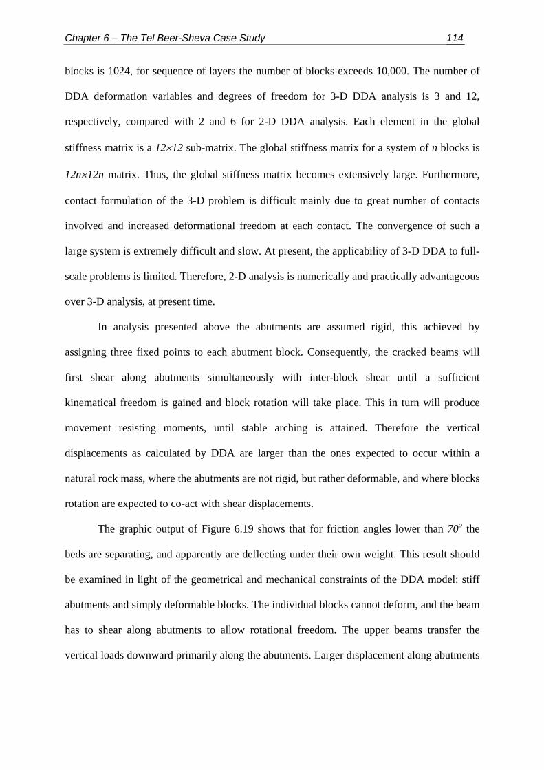
Chapter 6 – The Tel Beer-Sheva Case Study 114
blocks is 1024, for sequence of layers the number of blocks exceeds 10,000. The number of
DDA deformation variables and degrees of freedom for 3-D DDA analysis is 3 and 12,
respectively, compared with 2 and 6 for 2-D DDA analysis. Each element in the global
stiffness matrix is a 12×12 sub-matrix. The global stiffness matrix for a system of n blocks is
12n×12n matrix. Thus, the global stiffness matrix becomes extensively large. Furthermore,
contact formulation of the 3-D problem is difficult mainly due to great number of contacts
involved and increased deformational freedom at each contact. The convergence of such a
large system is extremely difficult and slow. At present, the applicability of 3-D DDA to full-
scale problems is limited. Therefore, 2-D analysis is numerically and practically advantageous
over 3-D analysis, at present time.
In analysis presented above the abutments are assumed rigid, this achieved by
assigning three fixed points to each abutment block. Consequently, the cracked beams will
first shear along abutments simultaneously with inter-block shear until a sufficient
kinematical freedom is gained and block rotation will take place. This in turn will produce
movement resisting moments, until stable arching is attained. Therefore the vertical
displacements as calculated by DDA are larger than the ones expected to occur within a
natural rock mass, where the abutments are not rigid, but rather deformable, and where blocks
rotation are expected to co-act with shear displacements.
The graphic output of Figure 6.19 shows that for friction angles lower than 70o the
beds are separating, and apparently are deflecting under their own weight. This result should
be examined in light of the geometrical and mechanical constraints of the DDA model: stiff
abutments and simply deformable blocks. The individual blocks cannot deform, and the beam
has to shear along abutments to allow rotational freedom. The upper beams transfer the
vertical loads downward primarily along the abutments. Larger displacement along abutments
Chapter 6 – The Tel Beer-Sheva Case Study 115
allows larger rotational freedom, and consequently larger mid-span deflection. Based on these
insights the deflection under own weight assumption should be ruled out.
The jointed layers are modeled such that each layer is free to shear along the
abutments. In the field the layers only partially comply with the model, since individual end
blocks may be supported by the abutments, forming a structure of cantilever beams, which
consequently reduce the active span. However, the relatively dense jointing of the Gareb
chalk (ca. 0.25m) minimizes this effect.
The first order displacement approximation in DDA results in constant strain/stress
elements, and stress concentrations within the blocks are not computed. The stability of the
beams however is achieved through rotation, which must produce stress concentration at the
contacts. Moreover, in weak rocks such stress concentrations can lead to failure of the intact
rock, thus to changes in contacts size and stiffness, which in turn can lead to further
deterioration of the individual blocks integrity and overall structural stability. A complete
stress distribution for the entire modeled region is not available. This shortcoming is acute
when the individual blocks are large. However for small blocks the stresses within the blocks
are nearly constant. Thus for a system consisting of a large number of small blocks, as in the
case of Tel Beer-Sheva, the stress distribution is assumed to be modeled with adequate
accuracy.
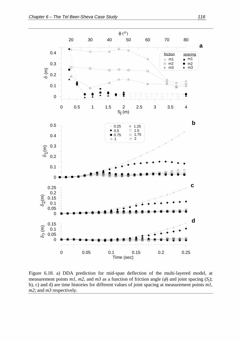
Chapter 6 – The Tel Beer-Sheva Case Study 116
20 30 40 50 60 70 80φ (ο)
0
0.1
0.2
0.3
0.4δ
(m)
0 0.5 1 1.5 2 2.5 3 3.5 4Sj (m)
m1m2m3
frictionm1m2m3
spacing
00.05
0.10.15
0.20.25
δ 2(m
)
0 0.05 0.1 0.15 0.2 0.25Time (sec)
00.05
0.10.15
δ 3 (m
)
0
0.1
0.2
0.3
0.4
0.5
δ 1(m
)
0.250.50.75
1.251.51.75
1 2
a
b
c
d
Figure 6.18. a) DDA prediction for mid-span deflection of the multi-layered model, at measurement points m1, m2, and m3 as a function of friction angle (φ) and joint spacing (Sj); b), c) and d) are time histories for different values of joint spacing at measurement points m1, m2; and m3 respectively.

Chapter 6 – The Tel Beer-Sheva Case Study 117
a)
b)
Figure 6.19. DDA graphic output of the multi-layer deformation for different values of joint friction angle: a) original geometry; b) φav = 30o.

Chapter 6 – The Tel Beer-Sheva Case Study 118
c)
d)
Figure 6.19. (cont.) DDA graphic output of the multi-layer deformation for different values of joint friction angle: c) φav = 50o; and d) φav = 70o.

Chapter 6 – The Tel Beer-Sheva Case Study 119
6.6.6. Comparison between DDA and classic Voussoir solutions
Stability analysis of the Tel Beer – Sheva water reservoir showed that the classic
Voussoir analysis is unconservative. Voussoir analysis predicts stability for friction angles of
φav > 20o, but with a peak friction angle of φp = 47o the roof has failed. DDA analysis for a single
layer with multiple joints showed that stability is assured for friction angles of φav > 75o. Clearly
DDA prediction is more accurate, albeit conservative (refer to previous section). The mode of
failure of the multi-jointed beam is clearly shown in Figure 6.16: maximum inter block shear
developed at the mid span, whereas at the abutments block rotation attained maximum value. This
mode of failure can be regarded as sagging. DDA showed that when the shear resistance along
joints is increased stability is achieved through increased rotation of blocks near the abutments.
Investigation of block size effect showed that the beam stability improves for blocks with high
aspect ratio; thus the findings of Passaris et al., (1993) are confirmed.
DDA showed that for the case of Tel Beer-Sheva analysis of the immediate roof (i.e.
single layer) is only partially applicable, given the fact that at least a portion of the vertical
load was transmitted vertically rather than laterally to the abutments. The stability of the
laminated Voussoir is governed by similar processes: stability is achieved when shear
resistance is sufficient to induce rotation of individual blocks close to the abutments. Then the
global behavior of the layers is changed from a succession of layers each imposing vertical
load on the layers below, to a coherent beam where loads are transformed laterally to the
abutments. This transition is indicated by almost uniform deflection of the individual layers
across the bulk of the sequence (Figure 6.18). Therefore the solution obtained by DDA using
a single layer configuration seems to be unconservative, suggesting that a mult-layer analysis
is warranted.

Chapter 7 – Stability analysis of underground openings 120
Chapter 7 - Stability Analysis of Underground Openings in Horizontally Stratified and Vertically Jointed Rock
7.1. Introduction
In the previous chapters the validation of DDA using analytical solutions, physical
models, and a case study were discussed, and the advantages of DDA over the classic
Voussoir model were shown. Furthermore, it was shown that DDA accounts for variations in
joint spacing and shear resistance (friction) along joints, leading to different modes of failures
and amount of deflection. Therefore, with given joint spacing and joint friction angle the
stability of underground openings in discontinuous rock can be assessed.
Lee et al., (2003) showed that when two joint sets are encountered at a tunnel
excavation face, the most critical joint combination consists of a set of horizontal joints
(bedding planes) intersecting vertical joints. Furthermore, they have shown that the
displacement of a key block at the roof tends to increase as the block size decreases.
However, no particular reference is made by Lee et al., to joint spacing and tunnel
dimensions.
This chapter explores the stability of underground openings excavated in horizontally
stratified and vertically jointed rock masses. This study concentrates on:
1. The effect of joint spacing and shear resistance on the height of
loosening above the excavation.
2. The relation between joint spacing and excavation span.

Chapter 7 – Stability analysis of underground openings 121
The paramount uncertainty associated with modeling discontinuous rock masses lies
with the geometrical structure of the rock mass, e.g. joints length and spacing distributions.
The main difficulty arises from the fact that most of the data regarding these parameters are
collected either from boreholes or from limited surface exposures; in rare cases exploratory
tunnels are excavated. The extrapolation from limited field data to a conceptual model of the
rock mass and then to a numerical model introduces further uncertainties.
Joint spacing, defined as the perpendicular distance between two neighboring
discontinuities, has been widely explored over the past three decades, and various techniques
for data collection and analysis were proposed (refer to Priest, 1993). It was found that within
a given joint set the joint spacing follows certain distribution laws, such as: normal, log-
normal, and negative exponential among others. It has also been suggested that joint spacing
is related to bed thickness, genesis, and geological setting (refer to Wu and Pollard, 1995).
The distribution law reflects this, as well as the measuring and analysis technique. Similar
findings were reported on issues of joint length (Zhang and Einstein, 1998; Mauldon, 1998).
In the current research the modeled rock mass is synthetic, with no reference to a
particular, naturally occurring rock-mass. The discontinuous rock-mass was generated using
the one-dimensional perturbation algorithm proposed by Shi and Goodman (1989). The
algorithm inputs are: the average joint spacing Sj, the average joint length Lj, the average joint
bridge Bj and the degree of randomness 210 << rD . When
21
=rD a full perturbation is
applied, when no perturbation is applied. The distribution function is assumed
uniform, for simplicity.
0=rD
7.1.1. Model geometry and mechanical properties
The analysis domain is 50m high and 40m wide. The opening geometry is of a
horseshoe shaped tunnel (Figure 7.1), with span B = 2a and height ht = b+c. Fixed boundaries
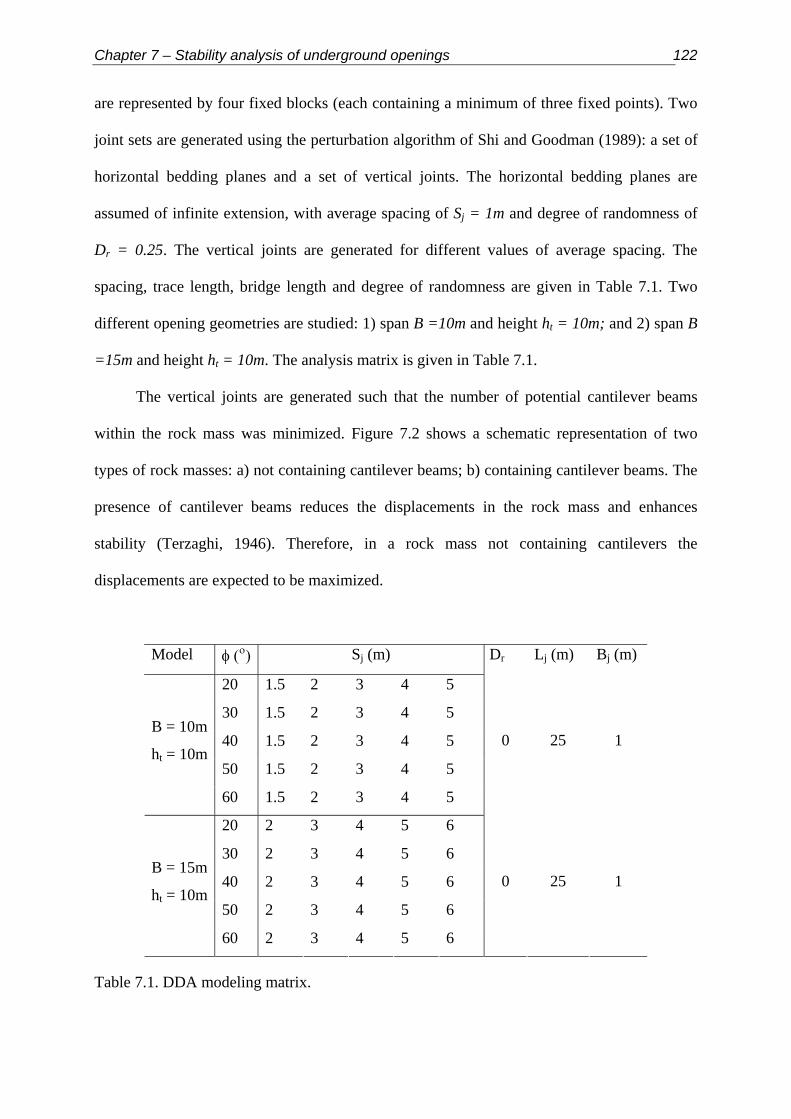
Chapter 7 – Stability analysis of underground openings 122
are represented by four fixed blocks (each containing a minimum of three fixed points). Two
joint sets are generated using the perturbation algorithm of Shi and Goodman (1989): a set of
horizontal bedding planes and a set of vertical joints. The horizontal bedding planes are
assumed of infinite extension, with average spacing of Sj = 1m and degree of randomness of
Dr = 0.25. The vertical joints are generated for different values of average spacing. The
spacing, trace length, bridge length and degree of randomness are given in Table 7.1. Two
different opening geometries are studied: 1) span B =10m and height ht = 10m; and 2) span B
=15m and height ht = 10m. The analysis matrix is given in Table 7.1.
The vertical joints are generated such that the number of potential cantilever beams
within the rock mass was minimized. Figure 7.2 shows a schematic representation of two
types of rock masses: a) not containing cantilever beams; b) containing cantilever beams. The
presence of cantilever beams reduces the displacements in the rock mass and enhances
stability (Terzaghi, 1946). Therefore, in a rock mass not containing cantilevers the
displacements are expected to be maximized.
Model φ (ο) Sj (m) Dr Lj (m) Bj (m)
20 1.5 2 3 4 5
30 1.5 2 3 4 5
40 1.5 2 3 4 5
50 1.5 2 3 4 5
B = 10m
ht = 10m
60 1.5 2 3 4 5
0 25 1
20 2 3 4 5 6
30 2 3 4 5 6
40 2 3 4 5 6
50 2 3 4 5 6
B = 15m
ht = 10m
60 2 3 4 5 6
0 25 1
Table 7.1. DDA modeling matrix.

Chapter 7 – Stability analysis of underground openings 123
The displacements within the rock mass are measured at seven measurement points
along a vertical line rising from the excavation crown. The locations of the measurement
points are given in Table 7.2.
Mechanical properties of the intact rock material are chosen to conform to “average”
values of sedimentary rocks. The mechanical properties of the intact rock material and
numeric control parameters are given in Table 7.3. The shear resistance along discontinuities
was assumed purely frictional; cohesion and tensile strength are assumed zero. The
discontinuities represent clean planar joints without surface roughness, wall annealing or
infilling. The friction angle for bedding planes and vertical joints is assumed equal for
simplicity; this is by no means limitation of the DDA method or its numeric implementation.
Measurement point x,y coordinates (m) Remarks
mp1 0, 0 excavation crown
mp2 0, 4.5
mp3 0, 8.5 center of domain
mp4 0, 13.5
mp5 0, 18
mp6 0, 23
mp7 0, 28
Table 7.2 Locations of measurement points in DDA model. x,y coordinates are with respect to excavation crown.
Density 2500 kg/m3
Elastic Modulus 10000 MPa
Poisson’s ratio 0.25
Penalty stiffness (g0) 1000 MN/m
Time step size (g1) 0.0002 - 0.0004 sec (1)
Penetration control parameter (g2) 0.0002
Dynamic control parameter (k01) 1
Table 7.3. Material properties and numeric control parameters for DDA model. (1) Time step size was adjusted to avoid numerical problems.

Chapter 7 – Stability analysis of underground openings 124
a
c
b
fixed point
measurmentpoint
Sj
Sb
0,0
x
y
Figure 7.1.Geometry of the DDA model.
Abutments
Rock blocks
cantilever blocks
a
b
Figure 7.2. Two types of rock masses: a) not containing cantilever beams; b) containing cantilever beams.

Chapter 7 – Stability analysis of underground openings 125
7.1.2. Selection of contact stiffness
In sections 4.2, 5.3.3 and 6.6.1 it was shown that the accuracy of DDA solution depends
on proper selection of numerical control parameters. Given a sufficiently small time step (g1)
and penetration control parameter (g2), the nature of the DDA solution is determined by inter-
block contact stiffness (g0). It was shown that when the number of blocks is large the contact
stiffness should be chosen such that that convergence of numerical solution is achieved.
In the current model the maximum number of blocks for analysis was 1102 (for Sj = 1.5
m). A sensitivity analysis was performed for this specific geometric configuration. The
maximum time step size was set to g1 = 0.0004 sec, the penetration control parameter was set
to g2 = 0.0002, and the number of time steps was n = 2500. The contact stiffness was
changed from g0 = 250 MN/m to g0 = 1000 MN/m. The results of the sensitivity study are
presented in Figure 7.3.
Figure 7.3a shows three time histories for different values of contact stiffness. When g0
= 250 MN/m the solution is clearly non-converging within the time span, with a “wave
length” of approximately 1500 time steps. Setting g0 = 750 MN/m changes the solution; the
oscillatory nature of an equilibrium solution is clearly visible. The “wave length” and
amplitude of oscillations are reduced implying smaller initial perturbation and faster
convergence. Increasing the contact stiffness to g0 = 1000 MN/m enhances the convergence,
and shows two pronounced modes of displacement. At the crown progressive deflection is
taking place, while at all other measurement points the deflection attains equilibrium position.
Figure 7.3b shows the number of open close iterations over computation time. For g0 =
250 MN/m the average number of iterations per time step is iav = 2.61, for g0 = 750 MN/m the
average number of iterations is iav = 3.11, and for g0 = 750 MN/m the average number of
iterations is iav = 3.22. Increasing the contact stiffness slightly impends on the numerical

Chapter 7 – Stability analysis of underground openings 126
efficiency. Based on these observations the contact stiffness value chosen for the analysis is
g0 = 1000 MN/m.
0.5
0.4
0.3
0.2
0.1
0
δ (m
)
0.5
0.4
0.3
0.2
0.1
0
δ (m
)
0 500 1000 1500 2000 2500time step
0.5
0.4
0.3
0.2
0.1
0
δ (m
)
g0=250 MN/m
g0=1000 MN/m
g0=750 MN/m
+28.5m+23.5m+18.5m+13.5m+8.5m+4.5mcrown
Figure 7.3. Contact stiffness sensitivity analysis for a DDA model of tunnel span B = 10m and vertical joints spacing Sj = 1.5: a) vertical deflections (δ) for different values of. Maximum time step size to g1 = 0.0004 sec, penetration control parameter g2 = 0.0002

Chapter 7 – Stability analysis of underground openings 127
1
2
3
4
5
itte
ratio
ns
1
2
3
4
5
itte
ratio
ns
0 500 1000 1500 2000 2500
1
2
3
4
5
itte
ratio
ns
g0 = 250 MN/m
g0 = 750 MN/m
g0 = 1000 MN/m
2.61
3.11 3.22
0 250 500 750 1000 1250stiffness (MN/m)
1
2
3
4
i av
6000
7000
8000
9000
tota
l nu
m. o
f itte
ratio
ns
6521
77848060
Figure 7.3. (cont.). Contact stiffness sensitivity analysis for a DDA model of tunnel span of B = 10m and vertical joints spacing of Sj = 1.5: b) iteration time history for different values of contact stiffness.
7.1.3. Criteria for stable arching
The displacement curves in Figure 7.3a show two modes of deformation: 1) increasing
displacement with time (measurement point 1); and 2) equilibrium position, after an initial
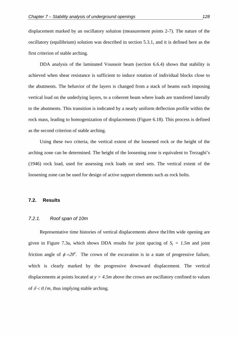
Chapter 7 – Stability analysis of underground openings 128
displacement marked by an oscillatory solution (measurement points 2-7). The nature of the
oscillatory (equilibrium) solution was described in section 5.3.1, and it is defined here as the
first criterion of stable arching.
DDA analysis of the laminated Voussoir beam (section 6.6.4) shows that stability is
achieved when shear resistance is sufficient to induce rotation of individual blocks close to
the abutments. The behavior of the layers is changed from a stack of beams each imposing
vertical load on the underlying layers, to a coherent beam where loads are transfered laterally
to the abutments. This transition is indicated by a nearly uniform deflection profile within the
rock mass, leading to homogenization of displacements (Figure 6.18). This process is defined
as the second criterion of stable arching.
Using these two criteria, the vertical extent of the loosened rock or the height of the
arching zone can be determined. The height of the loosening zone is equivalent to Terzaghi’s
(1946) rock load, used for assessing rock loads on steel sets. The vertical extent of the
loosening zone can be used for design of active support elements such as rock bolts.
7.2. Results
7.2.1. Roof span of 10m
Representative time histories of vertical displacements above the10m wide opening are
given in Figure 7.3a, which shows DDA results for joint spacing of Sj = 1.5m and joint
friction angle of φ =20ο. The crown of the excavation is in a state of progressive failure,
which is clearly marked by the progressive downward displacement. The vertical
displacements at points located at y > 4.5m above the crown are oscillatory confined to values
of δ < 0.1m, thus implying stable arching.
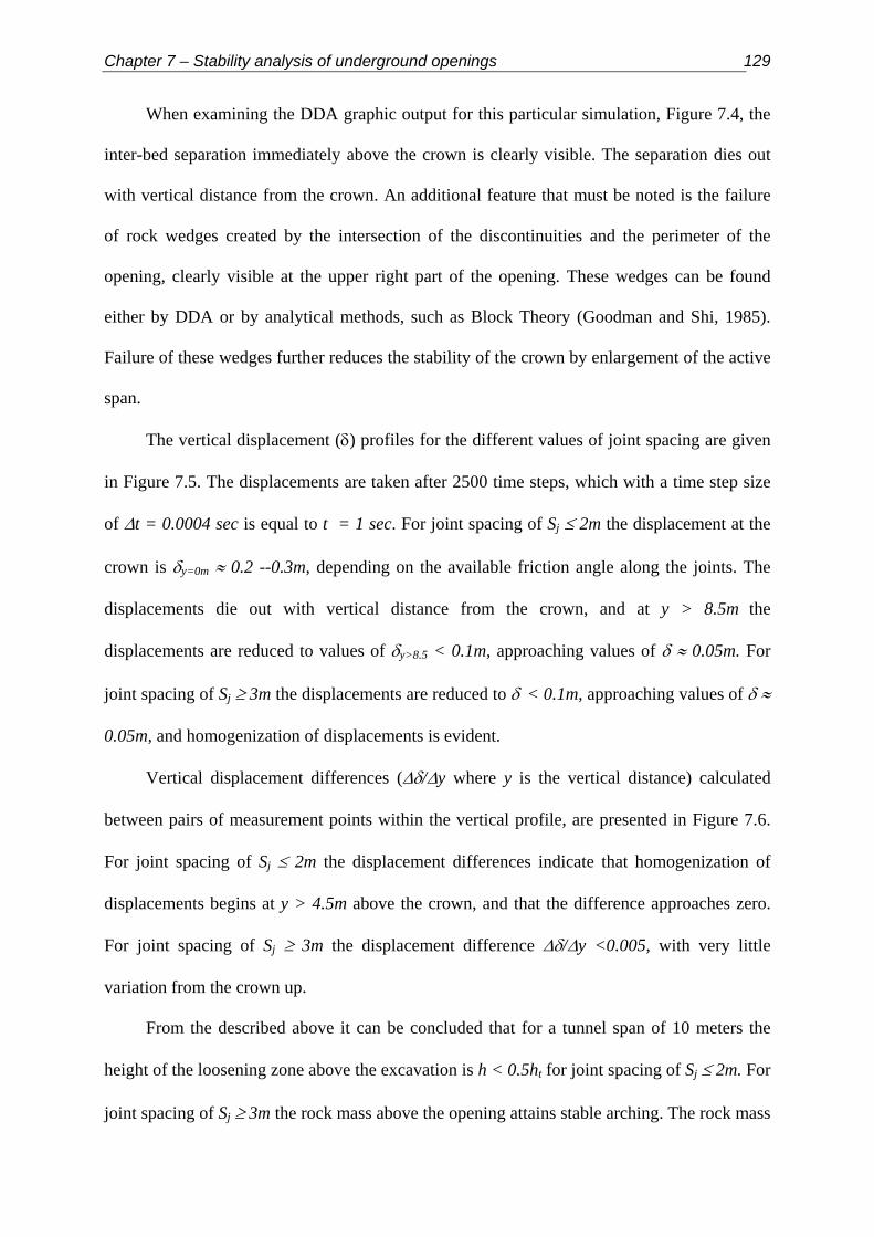
Chapter 7 – Stability analysis of underground openings 129
When examining the DDA graphic output for this particular simulation, Figure 7.4, the
inter-bed separation immediately above the crown is clearly visible. The separation dies out
with vertical distance from the crown. An additional feature that must be noted is the failure
of rock wedges created by the intersection of the discontinuities and the perimeter of the
opening, clearly visible at the upper right part of the opening. These wedges can be found
either by DDA or by analytical methods, such as Block Theory (Goodman and Shi, 1985).
Failure of these wedges further reduces the stability of the crown by enlargement of the active
span.
The vertical displacement (δ) profiles for the different values of joint spacing are given
in Figure 7.5. The displacements are taken after 2500 time steps, which with a time step size
of ∆t = 0.0004 sec is equal to t = 1 sec. For joint spacing of Sj ≤ 2m the displacement at the
crown is δy=0m ≈ 0.2 --0.3m, depending on the available friction angle along the joints. The
displacements die out with vertical distance from the crown, and at y > 8.5m the
displacements are reduced to values of δy>8.5 < 0.1m, approaching values of δ ≈ 0.05m. For
joint spacing of Sj ≥ 3m the displacements are reduced to δ < 0.1m, approaching values of δ ≈
0.05m, and homogenization of displacements is evident.
Vertical displacement differences (∆δ/∆y where y is the vertical distance) calculated
between pairs of measurement points within the vertical profile, are presented in Figure 7.6.
For joint spacing of Sj ≤ 2m the displacement differences indicate that homogenization of
displacements begins at y > 4.5m above the crown, and that the difference approaches zero.
For joint spacing of Sj ≥ 3m the displacement difference ∆δ/∆y <0.005, with very little
variation from the crown up.
From the described above it can be concluded that for a tunnel span of 10 meters the
height of the loosening zone above the excavation is h < 0.5ht for joint spacing of Sj ≤ 2m. For
joint spacing of Sj ≥ 3m the rock mass above the opening attains stable arching. The rock mass

Chapter 7 – Stability analysis of underground openings 130
response is dictated by the joint spacing and to a lesser extent by joint friction, for the
modeled range of friction angles. Only in one case, Sj = 2m and φ = 60o, the friction angle
inhibit excessive deflections and induce stable arching. Where the joint spacing is sufficiently
large stable arching is independent of friction angle. The findings of this section are
summarized in Table 7.4.
Friction angle (o)
20 30 40 50 60
1.5 < 0.45 < 0.45 < 0.45 < 0.45 < 0.45
2 < 0.45 < 0.45 < 0.45 < 0.45 Stable
3 Stable Stable Stable Stable Stable
4 Stable Stable Stable Stable Stable
Join
t spa
cing
(m)
5 Stable Stable Stable Stable Stable
Table 7.4. Normalized height of loosening zone (hr = h/ht) above an underground opening for a horseshoe tunnel of width B = 10m and height ht = 10m.
7.2.2. Influence of joint randomness
Modeling the transverse joints as long, perfectly persistent and with constant spacing
results in a rock mass structure with a minimum number of cantilever blocks. In this
configuration the deflections above the underground opening are expected to attain maximum
values. However, joints are seldom persistent, and statistical variations are to be expected. In
order to study the effect of joint variability on rock mass response the simulations for joint
spacing of Sj = 1.5m are repeated, with the following changes with respect to the transverse
joints: trace length Lj = 5m, bridge length Bj = 0.5m and degree of randomness of Dr = 0.25.
All other mechanical and geometrical parameters are kept the same. The results of the
simulations and comparison with the “uniform” simulation are presented in Figure 7.7. The
graphic output of the simulation for friction angle along joints of φ = 20ο is given in Figure
7.8.

Chapter 7 – Stability analysis of underground openings 131
Figure 7.4. DDA graphic output for tunnel span of B = 10m and vertical joint spacing of Sj = 1.5: a) initial configuration (top); b) deformed configuration (bottom).
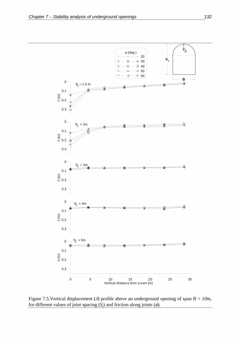
Chapter 7 – Stability analysis of underground openings 132
0.3
0.2
0.1
0
δ (m
)
φ (deg.)2030405060
0.3
0.2
0.1
0
δ (m
)
0.3
0.2
0.1
0
δ (m
)
0.3
0.2
0.1
0
δ (m
)
0 5 10 15 20 25 30Vertical distance from crown (m)
0.3
0.2
0.1
0
δ (m
)
Sj = 1.5 m
Sj = 2m
Sj = 3m
Sj = 4m
Sj = 5m
B
ht
δ
Figure 7.5.Vertical displacement (δ) profile above an underground opening of span B = 10m, for different values of joint spacing (Sj) and friction along joints (φ).

Chapter 7 – Stability analysis of underground openings 133
0
0.01
0.02
0.03
0.04
0.05
∆δ/ ∆
y
φ (deg.)2030405060
0
0.01
0.02
0.03
0.04
0.05
∆δ/ ∆
y
0
0.01
0.02
0.03
0.04
0.05
∆δ/ ∆
y
0
0.01
0.02
0.03
0.04
0.05
∆δ/ ∆
y
5 10 15 20 25vertical distance from crown (m)
30
0
0.01
0.02
0.03
0.04
0.05
∆δ/ ∆
y
Sj = 1.5 m
Sj = 2m
Sj = 3m
Sj = 4m
Sj = 5m
B
ht
δ
Figure 7.6. Vertical displacement difference (∆δ/∆y) profile above an underground opening of span B = 10m, for different values of joint spacing (Sj) and friction along joints (φ).

Chapter 7 – Stability analysis of underground openings 134
Introduction of joint randomness reduces the vertical displacements. The downward
crown displacement is reduced from δy=0m ≈ 0.15 - 0.3m, depending on the available friction
angle along joints for non-random joints to δy=0m ≤ 0.06m for the same opening geometry with
random joint statistics, with no apparent influence of joint friction. The vertical displacement
difference immediately above the crown is reduced from ∆δ/∆y <0.04, depending on the
available joint friction angle, to ∆δ/∆y <0.005, with no apparent influence of joint friction.
The reduction of displacements and their homogenization, through the introduction of
joint variability is attributed to the combined action of the following factors:
1. Nominal enlargement of joint spacing - resulting in enlargement of the
Voussoir blocks and reduction of vertical displacements.
2. Presence of cantilever blocks – resulting in reduction of vertically
transformed loads within the rock mass, refer to Terzaghi (1946).
The two configurations described can be regarded as the end-members of the modeled
rock mass. The first end-member (uniform joints) is clearly conservative, whilst the second
end-member (non-uniform joints) is less conservative. The initial value of joint spacing for
the two realizations is Sj = 1.5m, which results in rather large Voussoir blocks and a relatively
small number of blocks in a single beam. Thus, introduction of joint randomness and nominal
enlargement of Voussoir blocks further improves the overall performance of the rock mass.
However, when joint spacing is small and the number of blocks in a single beam is relatively
large (as in the case of Tel Beer-Sheva) the influence of joint randomness on the overall
performance of the rock mass is expected to be weaker.

Chapter 7 – Stability analysis of underground openings 135
0 5 10 15 20 25 30
0.3
0.2
0.1
0
δ (m
)
friction angle (deg.)2030405060
0 5 10 15 20 25 30
0.3
0.2
0.1
0
δ (m
)
no random joints random joints
5 10 15 20 25 30vertical distance from crown (m)
0.06
0.04
0.02
0
∆δ/ ∆
v
5 10 15 20 25 3vertical distance from crown (m)
0
0.06
0.04
0.02
0
∆δ/ ∆
v
a
b
c
dno random joints random joints
Figure 7.7. Rock mass response above an underground opening of span B = 10m, and joint spacing of Sj = 1.5m: a) vertical displacements - non-random (Dr = 0) joint configuration; b) vertical displacement difference - non-random joint configuration; c) vertical displacements – random (Dr = 0.25) joint configuration; d) vertical displacement difference - random joint configuration.

Chapter 7 – Stability analysis of underground openings 136
Figure 7.8. DDA graphic output for tunnel span of B = 10m, vertical joint spacing of Sj = 1.5m with random statistics: a) initial configuration (top); b) deformed configuration (bottom).

Chapter 7 – Stability analysis of underground openings 137
7.2.3. Roof span of 15m
The vertical displacement profiles for the different values of joint spacing are given in
Figure 7.9, and the displacement difference profiles are given in Figure 7.10. Clearly,
enlarging the opening span by 50%, while keeping the height unchanged, modifies the rock
mass response. For joint spacing of Sj = 2m and friction angle of φ = 20o the crown (y = 0)
displacement is δ = 1.8m, at y = 4.5m the displacement is δ =-0.6m, and approaching δ =
0.2m at y >25m, which is the magnitude of crown displacement for opening span of B = 10m.
The graphic output for this particular case is given in Figure 7.11. It is clearly seen that the
rock mass immediately above the crown is sagging, and inter-bed separation is clearly
present. The height of the loosening zone encompasses at least eight successive beds above
the crown, compared with three successive beds for B = 10m case (Figure 7.12). Furthermore,
the larger span enhances failure of rock wedges formed by intersection of discontinuities and
excavation perimeter. Increasing the joint friction angle reduces the overall displacements; the
crown displacement for φ ≥ 30ο is δ < 0.6m, and approaches δ ≈ -0.2m for y > 4.5m.
Enlarging the joint spacing to Sj = 3m reduces the vertical displacements at the crown to
δ = 0.54m for φ = 20ο, δ = 0.38m for φ = 30ο, and δ < 0.25m for φ ≥ 40ο. The displacements
are reduced with vertical distance approaching δ = 0.1 m. For joint spacing of Sj ≥ 4
displacements are homogenized, decreasing with an increase in joint spacing to values of δ ≈-
0.1 m. Vertical displacement differences reveal similar trends: decreasing with increase of
joint spacing, and homogenization of displacements for Sj ≥ 4. The findings of this section are
summarized in Table 7.5.

Chapter 7 – Stability analysis of underground openings 138
2
1.6
1.2
0.8
0.4
0
δ (m
)
friction angle (deg.)2030405060
0.6
0.4
0.2
0
δ (m
)
0.6
0.4
0.2
0
δ (m
)
0.6
0.4
0.2
0
δ (m
)
0 5 10 15 20 25 30Vertical distance from crown (m)
0.6
0.4
0.2
0
δ (m
)
Sj = 2m
Sj = 3m
Sj = 4
Sj = 5
Sj = 6m
B
ht
δ
Figure 7.9. Vertical displacement (δ) profile above an underground opening of span B = 15m, for different values of joint spacing (Sj) and friction along joints (φ).

Chapter 7 – Stability analysis of underground openings 139
0
0.1
0.2
0.3
∆δ/ ∆
y
friction angle (deg.)2030405060
0
0.02
0.04
0.06
0.08
0.1
∆δ/ ∆
y
0
0.02
0.04
0.06
0.08
0.1
∆δ/ ∆
y
0
0.02
0.04
0.06
0.08
0.1
∆δ/ ∆
y
0 5 10 15 20 25vertical distance from crown (m)
0
0.02
0.04
0.06
0.08
0.1
∆δ/ ∆
y
Sj = 2 m
Sj = 3m
Sj = 4m
Sj = 5m
Sj = 6m
B
ht
δ
Figure 7.10. Vertical displacement difference (∆δ/∆y) profile above an underground opening of span B = 15m, for different values of joint spacing (Sj) and friction along joints (φ).

Chapter 7 – Stability analysis of underground openings 140
Figure 7.11. DDA graphic output for tunnel of span B = 15m, vertical joint spacing of Sj = 2m and friction angle of φ = 20o: a) initial configuration (top); b) deformed configuration (bottom).

Chapter 7 – Stability analysis of underground openings 141
Figure 7.12. DDA graphic output for tunnel of span B = 10m, vertical joint spacing Sj = 2 and friction angle of φ = 20o m: a) initial configuration (top); b) deformed configuration (bottom).
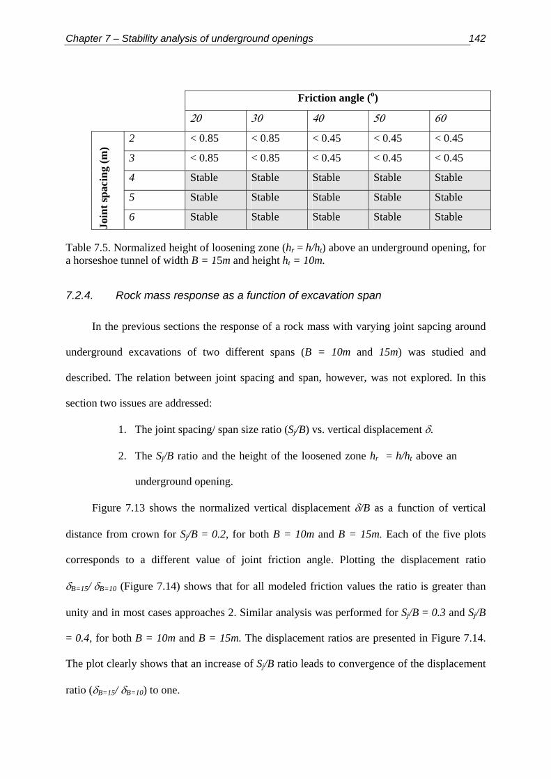
Chapter 7 – Stability analysis of underground openings 142
Friction angle (o)
20 30 40 50 60
2 < 0.85 < 0.85 < 0.45 < 0.45 < 0.45
3 < 0.85 < 0.85 < 0.45 < 0.45 < 0.45
4 Stable Stable Stable Stable Stable
5 Stable Stable Stable Stable Stable
Join
t spa
cing
(m)
6 Stable Stable Stable Stable Stable
Table 7.5. Normalized height of loosening zone (hr = h/ht) above an underground opening, for a horseshoe tunnel of width B = 15m and height ht = 10m.
7.2.4. Rock mass response as a function of excavation span
In the previous sections the response of a rock mass with varying joint sapcing around
underground excavations of two different spans (B = 10m and 15m) was studied and
described. The relation between joint spacing and span, however, was not explored. In this
section two issues are addressed:
1. The joint spacing/ span size ratio (Sj/B) vs. vertical displacement δ.
2. The Sj/B ratio and the height of the loosened zone hr = h/ht above an
underground opening.
Figure 7.13 shows the normalized vertical displacement δ/B as a function of vertical
distance from crown for Sj/B = 0.2, for both B = 10m and B = 15m. Each of the five plots
corresponds to a different value of joint friction angle. Plotting the displacement ratio
δB=15/ δB=10 (Figure 7.14) shows that for all modeled friction values the ratio is greater than
unity and in most cases approaches 2. Similar analysis was performed for Sj/B = 0.3 and Sj/B
= 0.4, for both B = 10m and B = 15m. The displacement ratios are presented in Figure 7.14.
The plot clearly shows that an increase of Sj/B ratio leads to convergence of the displacement
ratio (δB=15/ δB=10) to one.
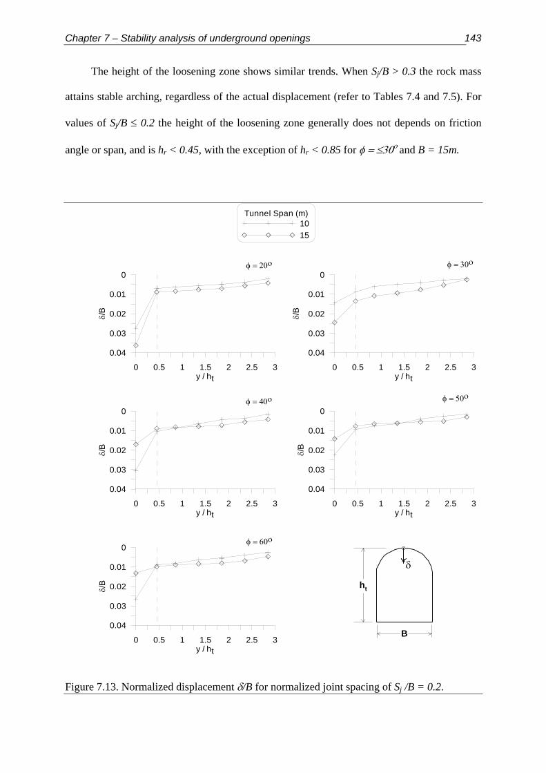
Chapter 7 – Stability analysis of underground openings 143
The height of the loosening zone shows similar trends. When Sj/B > 0.3 the rock mass
attains stable arching, regardless of the actual displacement (refer to Tables 7.4 and 7.5). For
values of Sj/B ≤ 0.2 the height of the loosening zone generally does not depends on friction
angle or span, and is hr < 0.45, with the exception of hr < 0.85 for φ = ≤30ο and B = 15m.
0 0.5 1 1.5 2 2.5 3y / ht
0.04
0.03
0.02
0.01
0
δ/B
0 0.5 1 1.5 2 2.5 3y / ht
0.04
0.03
0.02
0.01
0
δ/B
0 0.5 1 1.5 2 2.5 3y / ht
0.04
0.03
0.02
0.01
0
δ/B
0 0.5 1 1.5 2 2.5 3y / ht
0.04
0.03
0.02
0.01
0
δ/B
0 0.5 1 1.5 2 2.5 3y / ht
0.04
0.03
0.02
0.01
0
δ/B
Tunnel Span (m)1015
φ = 20ο φ = 30ο
φ = 40ο φ = 50ο
φ = 60ο
B
ht
δ
Figure 7.13. Normalized displacement δ/B for normalized joint spacing of Sj /B = 0.2.

Chapter 7 – Stability analysis of underground openings 144
0
1
2
3
4
δ(B
=15
) / δ
(B=1
0)
φ (deg.)20
30
4050
60
0
1
2
3
4
δ(B
=15
) / δ
(B=1
0)
0 0.5 1 1.5 2 2.5y / ht
3
0
1
2
3
4
δ(B
=15
) / δ
(B=1
0)
Sj / B = 0.2
Sj / B = 0.3
Sj / B = 0.4
a
b
c
Figure 7.14. Vertical displacement ratio δB=15/ δB=10: a) normalized joint spacing of Sj /B = 0.2; b) normalized joint spacing of Sj /B = 0.3; and c) normalized joint spacing of Sj /B = 0.4
Chapter 7 – Stability analysis of underground openings 145
7.3. Discussion
From the described above it can be concluded that for the modeled geometries the key
factor controlling the stability of underground openings excavated in horizontally layered and
vertically jointed rock mass is the spacing of vertical joints. The effect of friction along joints
is secondary, and is evident only when vertical joint spacing is lower than a certain threshold.
For underground openings with span of B = 10m the threshold is Sj ≤ 2m (Sj/B ≤ 1/5), whereas
for openings with span of B = 15m the threshold is Sj ≤ 3m (Sj/B ≤ 1/5). These thresholds are
functions of three factors: 1) joint spacing; 2) friction along joints; and 3) span opening.
When joint spacing is sufficiently large, the moments acting within each single block
are equilibrated, consequently leading to stable arching. This mechanism is self-regulating
and is independent of friction along joints. However, when joint spacing is bellow the
threshold value (Sj/B ≤ 1/5) the stability is determined by the interaction between joint spacing
and friction along joints. For an underground opening of span B = 10m and joint spacing of Sj
= 1.5m shear resistance along joints is not sufficient to preclude vertical displacements near
the excavation crown, indicating that thea rching mechanism is not fully developed. Stable
arching is only met at h > 0.45ht. For joint spacing of Sj = 2m and friction angle of
φ ≤ 50ο stable arching is met at h > 0.45ht’ as well. However, when the friction along joints is
φ = 60ο the shear resistance is sufficient to induce rotation of blocks and stable arching begins
at the crown.
For an underground opening of span B = 15m and joint spacing of Sj ≤ 3m the shear
resistance is not sufficient to induce block rotations and stable arching at the crown. Stable
arching is met at h > 0.85ht for φ ≤ 30ο and h > 0.45ht for φ >30ο. When Sj/B < 0.3 the

Chapter 7 – Stability analysis of underground openings 146
height of the loosening zone is h < 0.85ht, and in most cases is h < 0.45ht. When Sj/B > 0.3
stable arching begins at the crown. These findings are summarized in Table 7.6.
Sj/B hr Exceptions
≤ 0.2 < 0.45ht 1. Stable arching for B = 10m and φ = 60ο
2. <0.85ht for B = 15m and φ ≤ 30ο
0.3 0 Stable arching
0.4 0 Stable arching
Table 7.6. Normalized height of the loosening zone (hr = h/ht) above an underground opening for different values of joint spacing and opening span (Sj/B).
Given the modeled rock mass structure these estimates are clearly conservative. The
synthetic rock mass is designed such that resistance to downward displacement is provided by
shear resistance along joints, and that no cantilever beams are found within the rock mass.
Cantilever beams are expected in a natural rock mass, where joint geometry is characterized
by a certain statistical distribution. The presence of cantilever beams provides further
resistance to downward displacement. This effect is discussed in section 7.2.2: a simple linear
perturbation of joint spacing and bridge leads to reduction of vertical displacements and
induces stable arching. In a similar configuration with uniformly distributed joints arching is
achieved only at h > 0.45ht. Given the uncertainties associated with rock mass geometry and
its extrapolation, the extent of cantilever action cannot be easily quantified.
In this research the crushing strength of the rock was ignored, mainly since DDA is
currently not capable of modeling stress concentrations. Crushing occurs mainly in deep
excavations, in which the lateral compressive stresses are high. These stresses usually
preclude rock mass loosening. Crushing also occurs in weak rocks. In excavations at shallow
to moderate depths and competent rock, crushing failures are less common.
Chapter 7 – Stability analysis of underground openings 147
In terms of span B the height of the loosening zone is hr < 0.56B when Sj/B ≤ 0.2.
According to Terzaghi (1946) for tunnels excavated in a blocky rock mass (consists of
chemically intact or almost intact rock fragments, which are entirely separated from each
other and imperfectly interlocked) the expected overbreak ranges from 0.25B to 1.1(B+ht),
depending on the degree of jointing. However, a quantitative description of the degree of
jointing is not given.
Rose (1982) revised Terzaghi’s classification and described the degree of jointing in
terms of Rock Quality Designation of RQD (Deere et al 1967). According to Rose for a
moderately blocky rock mass (RQD = 75-85) the expected over break ranges from 0.25B to
0.2(B+ht), whereas for a very blocky rock mass (RQD = 30-75) the expected over break is
(0.2 to 0.6)(B+ht). This reduction was achieved by ignoring the level of water table, which
according to Brekke (1968) has little effect on rock load. The drawbacks of this revision are:
1) the friction along joints is neglected; 2) correlation with RQD.
RQD provides a quantitative estimate of rock mass quality from drill cores and is
defined as the percentage of intact rock pieces longer than 10cm in the total length of the core.
RQD is a directionally dependent parameter and its value may change considerably depending
on the borehole orientation. In a horizontally layered and vertically jointed rock mass the
RQD will be determined by the spacing between beds rather than the spacing of joints.
Furthermore, RQD is not sensitive for spacing greater than 10cm. For example, a drill core of
say 3m comprised of intact rock pieces each 10cm long will yield the same estimate as a
similar drill core comprised of 3 pieces each 1m long. Therefore, correlation with RQD is
problematic, especially for rock masses comprised of horizontal layers with vertical joints.
Comparison of the results of this research results with Terzaghi’s prediction shows that
the latter is conservative. Whereas Terzaghi’s classification scheme lacks a consistent
treatment of discontinuities, this research provides a systematic treatment of both joint

Chapter 7 – Stability analysis of underground openings 148
spacing and friction. Both joint spacing and friction angle along joints are easy to obtain
parameters, either in the field or in laboratory. Therefore, a prediction based on these
parameters is straightforward and explicit.

Chapter 8 - Conclusions 151
Chapter 8 – Conclusions
The purpose of this research was to study the stability of underground openings
excavated in horizontally layered and vertically jointed rock masses using the Discontinuous
Deformation Analysis (DDA) method. The objectives set forth in Chapter 1 of this thesis
were: 1) validation of the numeric Discontinuous Deformation Analysis (DDA) using
physical models and case studies; 2) investigation of the fractured beam kinematics; 3)
development of simplified design charts and tables for assessment of rock loads in
underground openings as function of joint spacing and joint friction angle.
DDA was validated using two different physical models: 1) shaking table model of a
single block on an incline performed by Wartman (1999) at University of California at
Berkeley; and 2) centrifuge model of a multi jointed single beam performed by Dr. M.
Talesnick at the Technion. The case study of Tel Beer-Sheva, originally investigated by
Hatzor and Benary (1998), was used to compare DDA and the classic Voussoir beam model,
and to study the kinematics of single and multi-layered fractured beams. Finally, the general
stability of underground openings excavated in a horizontally layered and vertically jointed
rock mass was studied, with particular reference to: 1) vertical joint spacing; 2) joint friction
angle; and 3) the relation between joint spacing and opening span.
Chapter 8 - Conclusions 152
8.1. DDA Limitations
In determining the applicability of DDA to a certain problem the assumptions and
limitations of the method should be recognized. With respect to stability analysis of
underground openings the following DDA limitations must be pointed out:
1. Two-dimensional formulation.
2. First order displacement approximation.
The reduction of three-dimensional field configurations to two-dimensional models and
the extrapolation from two-dimensional models to three-dimensional engineering conditions
is a known problem in rock engineering (Jing, 2003), and is beyond the scope of this thesis.
At present the main limitations of three-dimensional modeling of a discontinuous rock mass
are: the lack of maturity of three-dimensional models, and the requirement for excessive
computing power when modeling full-scale problems with a large number of discrete blocks.
A two-dimensional formulation provides computationally effective approximation to three-
dimensional engineering situations, it alsofaciliates large simulations and elaborate sensitivity
analysis.
DDA’s first order displacement approximation results in constant strain elements. Thus,
stress concentrations within the blocks are not modeled, nor is material damage. This
limitation is acute when modeling highly stressed rock masses, such as in deep excavations,
or when modeling deformation in weak rock. However, these particular conditions are not
relevant to the cases investigated here. The the reported results are applicable to moderately
shallow excavations, where the ambient stresses are low, and rock is relatively strong. In such
environments deformation is primarily achieved through rock block displacements rather than
by material damage.

Chapter 8 - Conclusions 153
8.2. DDA Accuracy
The accuracy of the DDA solution is determined by four control parameters:
1. Maximum time step size (g1).
2. Penetration control parameter (g2).
3. Contact spring stiffness (g0).
4. Dynamic control parameter (k01).
The control parameters g1 and g2 are interrelated; suitable guidelines for individual and
independent choice of each are not presented here. Throughout this research these parameters
were chosen to be of the same magnitude, for simplicity. It was found that given sufficiently
small g1 and g2, the accuracy of DDA is controlled by the value of the contact stiffness (the
penalty). The proper combination of these three control parameters insures proper
conditioning of the global stiffness matrix (i.e. diagonal dominance) and in turn assures
convergence of the solution. The influence of the dynamic controll parameter k01 is
discussed in section 8.3.
8.3. DDA Validation
When DDA solution is compared with analytical solutions for the block on an incline
problem the relative numeric error is found to be below 1.5%, indicating that block contact
algorithm in DDA is an accurate replication of the analytical model for frictional sliding.
When compared with a shaking table model for a block on an incline (Wartman, 1999) the
DDA solution is found to be conservative. The solution accuracy is improved by reducing the
dynamic control parameter, thus accounting for: 1) strain rate dependencies shown by the
particular interface used in this model; 2) difference between the numerical and physical

Chapter 8 - Conclusions 154
behavior at contact points during shaking; 3) lack of a physically sound energy dissipation
algorithm in DDA. It was found that a reduction of the inter time step velocity by 2% (setting
k01 = 0.98) improves both the ultimate accuracy and the kinematics of the DDA solution.
The main source of DDA numeric error is the initial perturbation of contact forces
associated with initial gravitational loading (Yeung, 1991; Doolin and Sitar, 2002). The
implicit time marching scheme of DDA (Newmark, 1959) dissipates this initial perturbation
through algorithmic damping, as the computation evolves with time. The magnitude of initial
perturbation, and consequently the numeric error, is inversely proportional to the contact
stiffness value. High contact stiffness results in lower initial perturbation and faster
convergence rate. An alternative strategy for enhancement of convergence is by introduction
of “kinetic damping”, namely reduction of inter time step transferred velocity. This strategy is
recommended when the mechanical system modeled is expected to attain equilibrium
position, or when the mode of failure is independent of system geometry, such as in block
sliding models. However, it should be remembered that “dynamic damping” is a numerical
manipulation, which is not related to a specific physical energy dissipation mechanism.
Validation of DDA using the block on an incline models, both analytical and physical,
is of prime importance to problems of slope stability, and as general benchmark tests for DDA
accuracy. However, they are of a limited applicability to underground openings, which
requires validation under more complex block contact conditions. During block sliding the
relative position of contacts is changed with time, but the contacts between the blocks, and
consequently contact forces and stresses within the blocks, are unchanged. This is not the case
for jointed beams spanning an underground opening. During beam deformation some of the
original contacts are expected to disappear while new contacts are expected to form, leading
to changes of contact forces between blocks and consequently of stresses within the blocks.
Chapter 8 - Conclusions 155
Centrifuge modeling of a multi-jointed rock beam comprised of six individual blocks,
showed that stable arching was achieved mainly through rotation of the external blocks. DDA
simulation of this particular model shows that stable arching is achieved through rotation of
stresses within the blocks, rather than by physical rotation of the external blocks. The
displacements predicted by DDA are found to be excessive, whereas the lateral forces
measured at the abutment are found to conform. The discrepancy between DDA and the
centrifuge models results from the geometrical Constraints of the DDA model. Whereas in the
centrifuge model the frictional interfaces allow block rotation, in the given DDA model the
infinitesimal thickness of the joints inhibits significant block rotation.
DDA analysis of a multi jointed rock beam, comprised of 32 individual blocks, shows
that given sufficient rotational freedom the deformation mode found in the centrifuge model
is replicated by DDA. The excessive rotations of the external blocks induce stable arching. It
is found that the transition from shear along abutments to block rotation and stable arching is
a function of the available shear resistance along joints. Given sufficient shear resistance, the
external blocks undergo rotation, which is found to be significantly larger when compared to
blocks found in the center of the beam. Otherwise, the external blocks shear along abutments,
and the magnitude of block rotations are found to be similar across the beam, indicating that
stable arching is not achieved.
Back analysis of an ancient roof failure in an underground water reservoir excavated in
horizontally layered and densely fractured rock mass, show that DDA successfully predicts
the anticipated failure. Back analysis of the ancient failure using the classic Voussoir model
shows that for the given rock mass this model was unconservative. The DDA model of the
particular excavation roof shows that within the layered roof the vertical loads transferred are
vertically from the upper stack to the lower members. The underlying assumption in the
Voussoir model, of complete detachment of the lower beam, is not satisfied in this case,

Chapter 8 - Conclusions 156
resulting in unconservative prediction regarding roof stability. It is found that in layered rock
masses the transition from unstable deformation to stable arching was marked by the
homogenization of vertical displacements within the rock mass, and that this transition is a
function of both transverse joint spacing and shear resistance along joints.
A DDA model of a multi-block system requires careful conditioning of the numeric
control parameters, since high contact stiffness impedes on solution convergence. Throughout
this research, it is found that contact stiffness is not associated with joint normal or tangential
stiffness, but rather is a numeric parameter. It is found that most accurate results are obtained
when contact stiffness lies between 102 MN/m to 103 MN/m, and the amplification factor g0/E,
where E is the block elastic modulus, is ranging from 0.05 to 1. When the contact stiffness
exceeds 103 MN/m the convergence of the solution rapidly deteriorates. Doolin and Sitar
(2003) reported that for the block on an incline problem the DDA solution converges for
amplification factors ranging from 0.1 to 100, and that the relative numeric error decreases for
higher penalty values. Given that the initial perturbation is inversely proportional to the
contact stiffness, the contact stiffness should be chosen such that both accuracy and
convergence are not compromised. For multi-block systems it is recommended that contact
stiffness should not exceed block material elastic modulus and that with increasing number of
blocks it should be decresed, until the solution converges.
8.4. Stability of Underground Openings in Horizontally Stratified and
Vertically Jointed Rock
The stability of underground openings excavated in a horizontally layered and vertically
jointed rock mass is studied using two different geometric configurations: 1) excavation span
B = 10m; and 2) excavation span B = 15m, for different values of transverse joint spacing and
friction angle along joints. A total number of 50 individual simulations is presented. It is
Chapter 8 - Conclusions 157
found that the height of the loosening zone above an underground excavation is determined
mainly by the ratio between joint spacing and excavation span (Sj/B). When Sj/B ≤ 0.2 the
height of the loosening zone is found to be smaller than 0.5B, with the exception of B = 15m
and φ ≤ 30ο where the height of the loosening zone extends to 0.85B. When Sj/B ≥ 0.3 the
rock mass above the excavation attains stable arching, reducing the loosening to unstable
wedges formed by the intersections of preexisting joints and the excavation perimeter.
The height of the loosening zone is inversely proportional to joint density. When the
number of blocks per beam (reciprocal to Sj/B) is greater than five (Sj/B ≤ 0.2) the beam tends
to deform by inter-block shear, while rotation is minimal. Consequently, the driving moment
generated by the vertical couple, including the vertical surcharge, is not equilibrated by
resisting moment generated by the lateral thrust, thus leading to progressive failure. When the
number of blocks per beam is equal or less than three (Sj/B ≥ 0.3), increased rotation generates
an effective lateral couple within each block, and the beam attains stable arching, after initial
deflection. For Sj/B = 0.3 the expected deflection of the excavation crown is δ ≈ 0.01B,
whereas for Sj/B = 0.4 the expected deflection of the excavation crown is δ ≈ 0.0075B.
These results are obtained for a synthetic rock mass constructed such that the number of
cantilever beams within it is minimal, achieved using constant joint spacing and long traces.
The reported displacements are therefore assumed to be conservative when compared to
naturally occurring rock masses. Introduction of simple variation algorithm on to the joint
generation routine reduces the displacements. This reduction is expected to attain maximum
effect for smaller values of joint spacing, since joint variability increases the nominal length
of the individual blocks and the “interlocking” within the rock mass.
Terzaghi’s rock load classification predicts that for a blocky rock mass the over break
height above the excavation ranges from 0.25B to 1.1(B+ht), depending on the degree of
jointing. However, the degree of jointing is not quantified, and guidelines for assessing the

Chapter 8 - Conclusions 158
degree of jointing are not provided. Rose’s revision (1982) limits the over break from 0.25B
to 0.6(B+ht), correlating the degree of jointing to RQD. The correlation between RQD and
joint spacing is ambiguous and can be misleading. In this research the expected over break is
correlated with joint spacing. It is found that the expected over break ranges from 0.45B to
0.85B for Sj/B ≤ 0.2, depending on the joint friction angle.
Terzaghi’s classification scheme lacks a consistent treatment of discontinuities. This
research provides a systematic treatment of both joint spacing and friction, which are readily
attainable parameters, either in the field or in laboratory. Therefore, a prediction based on
these parameters is straightforward and explicit.
8.5. Recommendations for Future Research
With reference to the main goal of this research, stability of underground openings in a
horizontally layered and vertically jointed rock mass, future research should address the
following issues and their effect on the stability of underground openings excavated in such a
rock mass:
1. The influence of block length to thickness ratio.
2. Different mechanical lithologies.
3. The effect of in-situ stresses, with special reference to deep
excavations.
4. The effect of cohesion and tensile strength along bedding planes and
joints.
5. Interaction of the rock mass and active support.
In this research the bedding planes are modeled as horizontal and the transverse joints
as vertical. This geometry is naturally occurring, however not exclusive. Other common rock
masses exhibit non-horizontal layering and inclined transverse joints. Previous research (e.g.

Chapter 8 - Conclusions 159
Lee et al., 2003) addressed the issue of joint inclination, without special reference to joint
spacing and shear resistance along joints. Future research should address the effect of joint
spacing and shear resistance along joints and bedding planes for different rock mass
geometries.
Future validation of DDA should focus on comparison between DDA models and full
scale engineering cases in complex geologic settings where rock mass deformation was
monitored and documented at complex geological settings. Successful comparison should
bring DDA’s potential to fulfillment, and transform it into an attractive analysis tool for the
practicing engineer.

Appendix 1 160
Appendix – Classic Voussoir Solution
The following is based on the original formulation of Evans (1941), modified and
corrected by Beer and Meek (1982). Configuration of the Voussoir beam and the notations are
given in Figure A1.
The basic assumptions of the analysis are:
1. The ground above the roof is completely distressed in the
direction normal to bedding.
2. The rock mass has parted along smooth bedding plane breaks
forming a series of beams.
3. The beam consists of no-tension material and the distribution of
compressive stress at the center and the abutments are linear.
The lateral couple formed by beam deflection equilibrates the overturning
gravitational-reaction couple
(A1) ZTSW=⋅
42
where W is the weight of the beam, S is the beams span, T is the axial thrust and Z is the lever
arm.
The structure presented in Fig. A1a is statically indeterminate since the lever arm Z is
not known. Assuming a parabolic reaction arch of length L and thickness Eq (A1) can
be written as
tn ⋅

Appendix 1 161
S
t
tnt
S4
W2
Z
fc
V
T
Mid-Span Crack
Voussoirblock
Abutment
a
b
Figure A1. a) Voussoir beam conceptual model; b) Voussoir beam notation.
(A2) 28
2 nZfS c=γ
where γ is beam unit weight.
The initial moment arm is given by 0Z
(A3) )321(0 ntZ −=
The length of the reaction arch L is given by
(A4) SZ
SL3
8 20+=
When the beam deforms the compression arch will shorten by
(A5) LEfL av=∆
where E is the beam elastic modulus and is the average stress along the compression
arch, given by
avf
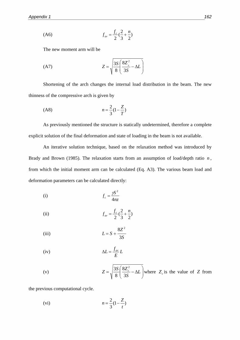
Appendix 1 162
(A6) )23
2(2
nff cav +=
The new moment arm will be
(A7) ⎟⎟⎠
⎞⎜⎜⎝
⎛∆−= L
SZSZ3
88
3 20
Shortening of the arch changes the internal load distribution in the beam. The new
thinness of the compressive arch is given by
(A8) )1(32
TZn −=
As previously mentioned the structure is statically undetermined, therefore a complete
explicit solution of the final deformation and state of loading in the beam is not available.
An iterative solution technique, based on the relaxation method was introduced by
Brady and Brown (1985). The relaxation starts from an assumption of load/depth ratio n ,
from which the initial moment arm can be calculated (Eq. A3). The various beam load and
deformation parameters can be calculated directly:
(i) nzSfc 4
2γ=
(ii) )23
2(2
nff cav +=
(iii) S
ZSL
38 2
+=
(iv) LEfL av=∆
(v) ⎟⎟⎠
⎞⎜⎜⎝
⎛∆−= L
SZSZ c
38
83 2
where is the value of from
the previous computational cycle.
cZ Z
(vi) )1(32
tZn −=

Appendix 1 163
The solution procedure involves sequential calculation of Eq. (i) to (v). Each cycle of
computation produces a new value of , which is then introduced in to Eq. (i) to restart the
solution cycle. Iterations of the solution sequence are continued until stable values of and
are obtained. Stable solution for is attained for minimum value of .
n
cf
n n cf
The factor of safety with respect to crushing at abutments ant at mid-span is given by
(A9) c
crushing fUCSSF =..
where is unconfined compressive strength. Factor of safety with respect to vertical
sliding along abutments and joints is given by
UCS
(A10) φγ
φ tantan..Snf
VTSF c
shear ==
where φ is friction angle.

References 164
References
Amadei, B., Lin, C., Dwyer, J. 1996. Recent extensions to the DDA method. In: Reza Salami, M., Banks, D. eds. Proceedings of the First International Forum on Discontinuous Deformation Analysis (DDA) and Simulations of Discontinuous Media, Berkley, California. TSI Press, Albuquerque. pp 1-30.
Barton, N., Lien, R., Lunde, J. 1974. Engineering classification of rock masses for the design of tunnel support. Rock. Mech. Rock. Eng. 6: 189-236.
Beer. G.and Meek, J.L. 1982. Design curves for roofs and hanging walls in bedded rock based on voussoir beam and plate solutions. Trans. Inst. Min. Metal. 91, A18-22.
Benari, R. 1996. Stability of underground openings in jointed chalky rock - a case study from Tel Beer-Sheva. M. Sc. Thesis, Department of Geological and Environmental Sciences. Ben Gurion University of the Negev. (in Hebrew)
Bieniawski, Z. T. 1973. Engineering classification of jointed rock masses. Trans. S. Afr. Inst. Civ. Eng. 15: 335-344.
Brady, B. H. and Brown, E. T. 1985. Rock mechanics for underground mining. 1st ed., George Allen and Unwin, London. 527 pp.
Brekke, T. L. 1968. Blocky and seamy rock mass in tunneling. Bull. Assoc. Eng. Geologist. 5 (1).
Bucky, P. B. 1931. Use of models for the study of mining problems. Am. Inst. Min. Met. Eng. Tech. Pub. 425, 28pp.
Bucky, P. B. and Taborelli, R. V. 1938. Effects of immediate roof thickness in longwall mining as determined by barodynamic experiments. Trans. Inst. Min. Metal. 130: 314
Chen, G. Miki, S. and Ohnishi, Y. (1996) Practical improvements to DDA. In: Reza Salami, M. & Banks, M. (eds.). Proceedings of the Firth International Forum on Discontinuous Deformation Analysis (DDA) and Simulation of Discontinuous Media. 97-110. TSI Press: Albuquerque.
Chugh, A. K. 1977. Stability analysis of jointed beam. Int. J. Numer. Ana. Methods Geomech. 1: 323-341.
Cundall, P. A. (1971). A computer model for simulating progressive, large scale movements in blocky rock system. Symposium of International Society of Rock Mechanics, Nancy, France. pp 11-18.

References 165
Deere, D. U., Hendron, A. J., Patton, F. D., and Cording, E. J. 1967. Design of surface and near-surface construction. In: C. Fairhurst (ed.) Failure and Breakage of Rock. Society of Mining Engineers of AIME, New York.
Desai, C. S., Zamman M. M., Lightner, J. G., Siriwardane, H. J. 1984. Thin layer element for interfaces and joints. Int. J. Numer. Anal. Methods Geomech. 8:19–43.
Diederichs, M. S. and Kaiser, P. K. 1999a. Stability of large excavations in laminated hard rock masses: the voussoir analogue revisited. Int. J. Rock. Mech. Min, Sci. 36: 97-117.
Diederichs, M. S. and Kaiser, P. K. 1999b. Authors' reply to Discussion by A.L. Sofianos Int. J. Rock. Mech. Min, Sci. 36 (7):995-997
Doolin, D and Sitar, N. (2002) Displacement accuracy of Discontinuous Deformation Analysis applied to sliding block. Journal of Engineering Mechanics, ASCE. 128(11): 1158-1168.
Economopuolus, J. N., Sofianos, A. I., Koronakis, N. J. 1994. Voussoir beam response of bedded limestone roofs in Greek underground mining excavations. Proceedings of the International Congress on Tunneling and Ground Conditions, Nasr City, Cairo, Egypt. pp 223-229.
Evans, W. H. 1941. The strength of undermined strata. Trans. Inst. Min. Metal. 50: 475-500.
Fayol, M. 1885. Sur les movements de terrain provoques par l’exploitation des mines. Bull. Soc. Indust. 14:818.
Ghaboussi, J., Wilson, E. L., Isenberg, J. 1973. Finite element for rock joints and interfaces. J. Soil Mech. Div. ASCE 99, SM10:833–848.
Goodman, R. E. 1989. Introduction to rock mechanics. 2nded. John Wiley & Sons. 562 pp.
Goodman, R. E. and Seed H. B. (1965) Earthquake induced displacements in sand embankments. J. Soil Mech. and Foundations Div. ASCE. 92(SM2): 125 – 146.
Goodman, R. E. and Shi, G-H. 1985. Block theory and its application to rock engineering. Prentice – Hall, New Jersey. 338p.
Goodman, R. E., Taylor, R. L., Brekke, T. L. 1968. A model for the mechanics of jointed rock. Journal of the Soil Mechanics Division, ASCE. 94 (SM3): 637-659.
Hatzor, Y. H. and Benary, R. 1988. The stability of a laminated voussoir beams: back analysis of a historic roof collapse using DDA. Int. J. Rock. Mech. Min, Sci. 35(2): 165-181.
References 166
Hatzor, Y. H. and Feintuch, A. (2001) The validity of dynamic block displacement prediction using DDA. Int. J. of Rock Mech. and Min. Sci. 38: 599 – 606.
Heyman, J. 1982. The masonry arch. Prentice Hall. 133 pp.
Hsiung, S-M. 2003. Discontinuous Deformation Analysis (DDA) with nth order polynomial displacement functions. in: Elsworth, D., Tinucci, J. P., Heasly, K. A. (ed.). Proceedings of the 38th US Rock Mechanics Symposium.
Jing L, Ma Y, Fang Z. 2001. Modeling of fluid flow and solid deformation for fractured rocks with discontinuous deformation analysis (DDA) method. Int. J. Rock Mech. Min. Sci. 38(3):343–55.
Ke. T-C. and Bray, J. D. 1995. Modeling of particulate media using discontinuous deformation analysis. J. Engrg. Mechanics. ASCE. 121(11): 1234 – 1243.
Kim, J., Bray, J. D., Reimer, M. F., Seed. R. B. (1999) Dynamic interface friction properties of geosyntetics. Unpublished report, University of California at Berkeley, Department of Civil Engineering.
Koo, C. Y.and Chern, J.C. 1996. The development of DDA with third order displacement functions. In: Reza Salami, M., Banks, D. eds. Proceedings of the First International Forum on Discontinuous Deformation Analysis (DDA) and Simulations of Discontinuous Media. Berkley, California. TSI Press, Albuquerque . 342-349.
Lauferr, H. 1958. Gebirgsklassifizierung fur den Stollenbau. Geologie und Bawesen. Vol. 24, No 1: 46-51.
Lee, D-H., Choo, S-K., Hong, C-S., Park, Y-J, Kim, G-J. 2003. A parametric study of the discontinuity in rock mass and its influence on tunnel behavior. Proceedings of the 10th ISRM Congress. South African Institute of Mining and Metallurgy. 745 – 748.
Lemos, J. V., Hart, R. D., Cundall, P. A. 1985. A generalized distinct element program for modeling jointed rock mass. In: Stefanson, O. ed. Proceedings of International Symposium on Fundamentals of Rock Joints. 335-343.
MacLaughlin, M. (1997) Discontinuous Deformation Analysis of the kinematics of rock slopes. Ph.D. thesis, Department of Civil Engineering, University of California, Berkley.
Mauldon, M. 1998. Estimating mean fracture trace length and density from observations in convex window. Rock. Mech. Rock. Eng. 31(4): 201-216.
McBride, A.and Scheele, F. (2001) Investigation of discontinuous deformation analysis using physical laboratory models. In: Bicanic, N. (ed.). Proc. of the Fourth International Conference on Discontinuous Deformation Analysis. 73-82.

References 167
Newmark, N. M. (1959) A method of computation for structural dynamics. J. of the Eng. Mech. Div. ASCE . 85( EM3)
Nomikos, P.P., Sofianos, A. I., and Tsoutrelis, C. E. 2002. Symmetric wedge in the roof of a tunnel excavated in an inclined stress field Int. J. Rock. Mech. Min. Sci.39 (1): 59-67
O’Sullivan, C. and Bray, J. D. (2001) A comparative evaluation of two approaches to discrete element modeling to particulate media. In: Bicanic, N. (ed.). Proceedings of the Fourth International Conference on Discontinuous Deformation Analysis. Glasgow, Scotland. 97-110.
Obert, L. and Duvall, W. I. 1976. Rock mechanics and the design of structures in rock. 1st ed. John Wiley. 650 pp.
Pacher, F., Rabcewicz, L. and Golser, J. 1974. Zum der seitigen Stand der Gebirgsklassifizierung in Stollen-und Tunnelbau. Proc. XXII Geomech. colloq., Salzburg, 51-58.
Passaris, E. K. S., Ran, J. Q., Mottahed, P. 1993. Stability of the jointed roof in stratified rock. Int. J. Rock. Mech. Min, Sci. Geomech. Abstr. 30(7): 857-860.
Pender, M. J. 1985. Prefailure joint dilatancy and the behavior of a beam with vertical joints. Rock. Mech. Rock. Eng. 18: 253-266.
Polishook, B.and Flexer, A. 1998. Assessment of chalk rock mass in excavation. Bull. Eng. Geol. Env. 57: 145-150.
Polishook. B. 1995. Geological and geomechanical properties of chalk and their influence on underground structures. Ph.D. Thesis. Tel Aviv University. (in Hebrew).
Priest, S. D. 1993. Discontinuity analysis for rock engineering. Chapman and Hall. 47 pp.
Ran, J. Q., Passaris, E. K. S., Mottahed, P. 1994. Shear sliding failure of the jointed roof in laminated rock mass. Rock. Mech. Rock. Eng. 27(4): 235-251.
Riedmüller, G. and Schubert, W. 1999. Critical comments on quantitative rock mass classifications. Felsbau. 17(3): 164-167.
Rose, D. 1982. Revising Terzaghi’s tunnel rock load coefficients. In: Goodman, R. E. and Hueze, F. (eds.). Proceedings of the 23rd Symposium on rock Mechanics. Berkeley, California. Society of Mining Engineers, AIMMP. 951-960.
Sepehr, K., and Stimpson, B. 1988. Roof deflections and sag in jointed horizontally bedded strata – a numerical study. Rock. Mech. Rock. Eng. 21: 207-218.

References 168
Sheorey, P.R. 1994. A theory for in situ stresses in isotropic and transversely isotropic rock. Int. J. Rock Mech. Min. Sci. & Geomech. Abstr. 31(1), 23-34.
Shi, G-H. 1988. Discontinuous Deformation Analysis – a new numerical method for the statics and dynamics of block system. Ph. D. Thesis, Department of Civil Engineering, University of California, Berkley. 378p.
Shi, G-H. 1993. Block System Modeling by Discontinuous Deformation Analysis. Topics in Engineering Vol. 11, Computational Mechanics Publications. 209p.
Shi, G-H. and Goodman, R. E. 1989. The key block of unrolled joint traces in developed maps of tunnel walls. Int. J. Numer. Ana. Methods Geomech. 13: 131-158.
Shingi, M. Ohno, H. Otsuka, Y. and Ma, G. (1997) Viscosity coefficient of the rock fall simulation. In. Ohnishi, Y (ed.). Second International Conference on Analysis of Discontinuous Deformation. Kyoto, Japan 201-210.
Sofianos , A. I. 1996. Analysis and design of underground hard rock voussoir beam roof. Int. J. Rock. Mech. Min. Sci. 33(2): 153-166.
Sofianos, A. I. 1999. Discussion of the paper by M.S. Diederichs and P.K. Kaiser "Stability of large excavations in laminated hard rock masses: the voussoir analogue revisited. Int. J. Rock. Mech. Min. Sci. 36(7): 991-993.
Sofianos, A. I., Kapenis, A. P., Rogakis, C. 1998. Voussoir beam analysis of underground marble quarry. In: Rosmanith, H. P. ed. Mechanics of jointed and Faulted rocks. Balkema. 515-520.
Sofianos, A. I.and Kapenis, A, P. 1998. Numerical evaluation of the response in bending of an underground hard rock voussoir beam roof. Int. J. Rock. Mech. Min, Sci. 35(8): 1071-1086.
Sterling, R. L. 1980. The ultimate load behavior of laterally constrained rock beams. In: Summers, D. A. ed. The state of the art in rock mechanics, Proc. 21st US Symp. Rock Mech. University of Rolla, Missouri. 533-542.
Talesnick, M.L. and Hatzor, Y. H. (in press). Determination of interface parameters between rock blocks in centrifuge models. Int. J. Rock. Mech. Min. Sci.
Taylor, R. N. 1995. Geotechnical centrifuge technology. Blackie Academic and Professional, Glasgow. pp 296.
Terzaghi, K. 1946 Rock defects and loads on tunnel support. In: Proctor, R. V., White, T., eds. Rock tunneling with steel supports. Commercial School and Stamping Co, Youngstown. pp 15-99.
Timoshenko, S. and Goodier, J. N. 1951. Theory of Elasticity. Engineering Societies Monographs. McGraw-Hill. 1951.

References 169
Tsesarsky, M. and Hatzor, Y, H. 2000. Stability of large span, shallow underground openings in soft discontinuous chalk. Proceedings of the Eurock 2000 Symposium, Aachen, Germany. 427-432.
Wang, C-Y., Chuang C-C. and Sheng, J. 1996. Time integration theories for the DDA method with Finite Element meshes. In: Reza Salami, M. & Banks, M. (eds.). Proceedings of the Firth International Forum on Discontinuous Deformation Analysis (DDA) and Simulation of Discontinuous Media. 97-110. Berkeley, California. TSI Press: Albuquerque.
Wartman, J. 1999. Physical model studies of seismically induced deformation of in slopes. Ph. D. Thesis, Department of Civil Engineering, University of California, Berkley.
Wartman, J., Bray, J. D. and Seed, R. B. 2003. Inclined plane studies of the Newmark sliding block procedure. Journal of Geotechnical and Geoenvironmental Engineering, ASCE. 129 (8): 673-684.
Wright, F. D. 1972. Arching action in cracked roof beams. Proceedings of the 5th Int. Strata Control. Conf. 29: 1-9.
Wright, F. D. 1974. Design of roof bolt patterns for jointed roof. Bureau of Mines, N.T.I.S. U. S. Department of Commerce.
Wu, H. and Pollard, D. D. 1995. An experimental study of relation between joint spacing and layer thickness. J. Struc. Geol. 6: 887-905.
Yeung, M. R. 1991. Application of Shi’s Discontinuous Deformation Analysis to the study of rock behavior. Ph. D. Thesis, Department of Civil Engineering, University of California, Berkley. 341p.
Zhang, L. and Einstein, H. H. 1998. Estimating the mean trace length of rock discontinuities. Rock. Mech. Rock. Eng. 31(4): 217-235.
Zienkiewicz, O. C., Best, B., Dullage, C., Stagg, K. 1970. Analysis of nonlinear problems in rock mechanics with particular reference to jointed rock systems. Proceedings of the Second International. Congress on Rock Mechanics, Belgrade, Yugoslavia.