stability prediction of multiple- teeth boring operations
TRANSCRIPT

Master's Degree Thesis
ISRN: BTH-AMT-EX--2013/D-08--SE
Supervisors: Martin Magnevall, AB Sandvik Coromant Ansel Berghuvud, BTH
Department of Mechanical Engineering
Blekinge Institute of Technology
Karlskrona, Sweden
2013
Amir Parsian
Stability Prediction of Multiple-Teeth Boring Operations


1
Stability Prediction of Multiple-Teeth Boring Operations
Amir Parsian
Department of Mechanical Engineering Blekinge Institute of Technology
Karlskrona, Sweden 2013
Thesis submitted for completion of Master of Science in Mechanical Engineering with emphasis on Structural Mechanics at the Department of Mechanical Engineering, Blekinge Institute of Technology, Karlskrona, Sweden.
Abstract
In many metal cutting operations, the relative displacement between the tool and the workpiece, determines the surface finish and the dimensional quality of the product. In an unstable operation, this relative displacement becomes bigger in an uncontrolled way and affects the cutting process. Vibrations of machine-tool systems leave a wavy surface in every tooth period. If waves on successive periods are not in phase, chip thickness may grow exponentially and cause an unstable operation. Having more than one cutting edge in boring tools can facilitate higher material removal rates and thereby boost productivity. Regenerative chatter vibrations, as a cause for instability in multiple-teeth boring operations, is investigated in this thesis. Different analyses for different types of inserts are presented. A method to approximate the uncut chip area is proposed to facilitate the frequency domain simulation. The proposed models were experimentally validated by cutting tests.
Keywords: Stability, Chatter vibration, Multiple-teeth boring, Variable pitch.

2
Acknowledgements
This work was carried out at the Department of Mechanical Engineering, Blekinge Institute of Technology, Karlskrona, Sweden, and at AB Sandvik Coromant, Sandviken, Sweden under the supervision of Dr. Ansel Berghuvud and Dr. Martin Magnevall.
I wish to express my deep gratitude and appreciation to Dr. Martin Magnevall for his great support during this thesis. His indispensable comments and kind advices were greatly helpful throughout the work.
I would like to thank Dr. Ansel Berghuvud for his guidance. I am also very grateful to him for his valuable lectures during my Master’s studies.
I would like to gratefully acknowledge financial support from AB Sandvik Coromant.
In addition, a thank you to Michael Ekeroth, who helped with the measurements.
Karlskrona, May 2013
Amir Parsian

3
Contents
1 Notation ................................................................................................... 4
2 Introduction ............................................................................................ 6
2.1. BACKGROUND .................................................................................... 6 2.2 AIM AND SCOPE OF THE THESIS ........................................................... 8
3 Chatter Vibration ................................................................................. 10
4 Boring Operation ................................................................................. 14
4.1. OVERVIEW ........................................................................................ 14 4.2. CUTTING FORCES AND STRUCTURAL DEFORMATIONS ...................... 17 4.3. CHIP FORMATION ............................................................................. 19 4.4. INSERTS ............................................................................................ 22
5 Modeling ............................................................................................... 25
5.1 INSERT TYPE 1 .................................................................................. 25 5.1.1 Time domain simulation ........................................................ 32 5.1.2 Frequency Domain Simulation .............................................. 35 5.1.3 Simulation in the Time and Frequency Domains ................... 41
5.2 INSERT TYPE 2 .................................................................................. 44 5.2.1 Exact Area Calculation .......................................................... 46 5.2.2 Area Approximation .............................................................. 51 5.2.3 Simulations in the Time and Frequency Domains ................. 56
6 Experimental Results ........................................................................... 58
6.1 FRF MEASUREMENTS (SYSTEM IDENTIFICATION) ............................ 58 6.2 MEASURING CUTTING FORCE COEFFICIENTS ................................... 60 6.3 MEASURING THE SOUND OF VIBRATIONS (MODEL VERIFICATION) .. 65
7 Variable Pitch Angles .......................................................................... 69
8 Discussion and Conclusion .................................................................. 71
9 References ............................................................................................. 74

4
1 Notation
Uncut chip area
Dynamic area
Remaining area
Depth of cut
Cutting edge length
Difference in the radial position after one tooth period
Force
Force component in the feed direction
Force component in the radial direction
Force component in the tangential direction
Force component in the direction
Total force in the , -plane
Force component in the direction
Force component in the direction
Feed per tooth
Chip thickness
Identity matrix
Cutting force coefficient for the feed direction
Cutting force coefficient for the radial direction
Cutting force coefficient for the tangential direction
Height of the insert
Cutting edge contact length
Number of cutting edges (inserts) on the tool
Spindle speed
Radial position

5
Root mean square
Revolutions per minute
Time
Time delay
Δ Radial displacement during one tooth period due to the radial vibration
Δ Infinitesimal change in the direction
Δ Infinitesimal change in the direction
Δ Infinitesimal change in the direction
Δ Infinitesimal change in angular position
Phase difference
Angle between and the tangential direction
Λ Eigenvalue
Transfer function
Angle between the cutting edge and the direction
Chatter frequency
6
2 Introduction
2.1. Background
Shaping materials is an important part of engineering and machining is one of the ways to make the final shape of products. In machining, a tool removes material from the workpiece to shape it into a desired form. Metals are more common in machining. Machining metals is also called metal cutting. There are different types of metal cutting operations. For example turning, milling, drilling and boring [1]. In addition, there are some non-traditional machining processes. For example, water jet, electrical discharge machining and laser machining. Many engineering products are made either directly or indirectly, by machining operations. In the rest of this report, for the sake of brevity, traditional machining operations to cut metals will be referred to as metal cutting. Interested readers may refer to [1,2,3] for more details about machining operations.
Boring is an operation to machine a hole that is produced in other processes such as casting, flame cutting, extrusion or forging [2]. Producing a hole with one of the mentioned methods and then using a boring tool to produce closer tolerances and higher surface finish can be more economic than solid drilling. In a boring operation, a rotating boring tool, in an axial movement, is fed through a hole to open it up [2]. Boring tools might have one or more than one cutting edges. In this work, boring operations that involve tools with more than one cutting edge are referred to as multiple-teeth boring operations.
Dynamic forces (that exist in all cutting operations) may cause vibration in the workpiece, the tool and the machine-tool structure. Vibrations encountered in metal cutting can be categorized into three groups according to Tobias [4]:
1- Free vibrations that might be due to external or internal shocks etc. In this case, external or internal transient, short time

7
excitations cause the system to vibrate. An example is the transmitted shocks from other operations such as pressing.
2- Forced vibrations that are caused by unbalanced spindles or masses on rotary parts etc. These forces usually produce periodic excitations on the system. The sources of these vibrations might be other machines that their vibrations are transmitted through the foundations.
3- Self-induced vibrations that are generated by either metal cutting operation itself or other mechanisms in the machine.
Chatter is a self-induced vibration phenomenon and can be generated by different mechanisms, where in most machining operations the dominant mechanism is regeneration of chip load [4]. In chatter vibrations, cutting forces grow during the operation [5] (See chapter 3). Chatter vibrations may occur in different metal cutting operations, for example milling, turning or boring. Since chatter vibrations cause poor surface finish, large cutting forces and low productivity [6], it is important to investigate their mechanism.
Tobias [4] was one of the pioneer who explained the fundamental theory behind chatter vibrations in an orthogonal cutting operation. Altintas et al. in [7] investigated chatter vibration in milling. In some previous works, the stability prediction for single edge boring operations is investigated [6,8]. Altintas et al. in [9] presented a frequency domain analysis for chatter stability prediction in plunge milling operations. Plunge milling operations for boring cylinders are similar to boring operations. One difference is that in plunge milling the depth of cut is usually more than boring operation. This causes less effect of nose radius on chatter stability. Ko and Altintas [10] proposed a mathematical model in the time domain to predict the cutting forces generated in plunge milling and it is suggested that chatter vibrations can be reduced by strengthening the flute cavities in tools in order to increase the torsional rigidity [10]. Mechanics of boring operations is studied in [11,12]. Lazoglu et al. in [13] studied dynamics of boring operations. Altintas et al. [14] investigated the effect of process damping on chatter stability. It is shown that when the tool is worn, the

8
process damping coefficient and the chatter stability limit increase [14]. Eynian, in a comprehensive study [15], showed how to measure and model process damping mechanism in metal cutting at low cutting speeds. Variable pitch angles can be employed to hinder the regenerative mechanism and consequently increase the process stability [16]. Budak [16,17] presented an analytical design method to increase the stability for milling cutters with variable pitch angles.
Determining the limiting depth of cut for stable operating conditions can significantly increase the performance of the metal cutting operation and thus the material removal rate. Using tools with multiple-teeth can also aid in increasing productivity [2]. This thesis focuses on stability prediction of multiple-teeth boring tools. Methods for predicting the limiting depth of cut of multiple-teeth boring tools are developed. The methods are applicable both in the time domain as well as in the frequency domain. For the time domain, a method is offered that uses exact area of the uncut chip and employs MATLAB SIMULINK® to perform the simulation. Different types of inserts need different analyses. In this thesis, the inserts are categorized into different types according to their geometry and suitable analyses are proposed for each type (See chapter 5).
Throughout this report, unstable operations refer to metal cutting operations that develop initial small disturbances into large vibrations and cause failure of the workpiece.
2.2 Aim and scope of the thesis
The main purpose of this thesis is to provide a fast simulating model to predict instability in multiple-teeth boring operations. The model is intended to be used for optimization of design parameters and aid in selecting appropriate cutting data.
For multiple-teeth boring operations, the aim of the work is to answer the following questions:

9
1- For a given set of cutting data, machine tool and workpiece dynamics, is the operation stable?
2- How does the geometry of the tool and the operation affect the stability of the operation?
3- How do the tool specifications such as number of teeth and their positions affect the stability of the operation?
4- How do dynamic behavior of the tool and the workpiece affect the stability of the operation?
5- Is it possible to make the operation more stable by changing the design parameters?
6- Is it possible to find a model that is fast enough in simulation to be used in optimization routines?
The obtained models are intended to cover a wide range of material and dynamic behaviors for the tool and the workpiece. This range should be wide enough to cover practical applications in the industry. The model should be applicable for different conventional designs and geometries for multiple-teeth boring tools.
The scope is narrowed to linear dynamic behaviors for each structure. For large deformations the structures becomes nonlinear. However, in an unstable operation, before reaching nonlinearity point, the workpiece fails due to poor surface finish resulting from uncontrolled large deformations. Therefore, nonlinearities in structural dynamics are not covered in this thesis.

3 C
Figure 3.1boring operatfundamentalssimple cuttindisplacement movement duharmonic mochip. In the lethe thicknessoperation onchip have a pthickness.
Figure 3.1.
Chatter V
1 shows chatttion. Chatter
of chatter vng operations
due to the statue to a time ovement produeft side of Figu of the chip the right side
phase differen
. Chatter mark
10
Vibratio
ter marks on avibration is a
vibrations theoare shown in
tic cutting forcdependent va
uces wavy surure 3.2, two wa
remains consof Figure 3.2
nce and this m
ks on a workpioperatio
n
a workpiece ma self-inducedory are discun Figure 3.2.ces, there is anariation of therfaces on bothaves are in phastant. On the 2, the waves omeans that the
iece made by aon.
made by an ud vibration [4ussed in [4,5]. In addition n additional hae cutting forceh sides of thease and conseqother hand,
n the surfaceschip have a v
an unstable bo
unstable 4]. The ]. Two to the
armonic e. This e uncut quently for the s of the varying
oring

Fig
A vforccausdiag
Fig
As proc
gure 3.2. Simp
variable uncut ces are affecteses variation gram in Figure
gure 3.3. A sim
shown in Figcess in a metal
Dy
thi
Wor
k pi
ece
ple cutting opein cu
chip thicknesed by the uncin the cutting
e 3.3.
mple block diaga
ure 3.4, an inl cutting opera
ynamic chip ickness
11
erations that shutting operatio
ss causes a varut chip area [
g forces. This
gram that showare generated.
nitial disturbanation.
Dynamic chip area
how how chatons.
riable chip are[5], variation s is shown in
ws how dynam
nce can trigge
Dynamcuttinforce
ter may develo
ea. Since cuttiin the chip a
n a simple blo
mic cutting forc
er a regenerat
mic ng es
op
ing area ock
ces
tive

12
Figure 3.4. Block diagram that shows how an initial disturbance can trigger a regenerative process.
Using Fourier analysis, the initial disturbance can be written as a summation of harmonics. Every harmonic can be analyzed separately, and then the total response of the system can be calculated by combining all harmonic responses.
The regenerative process shown in Figure 3.4 can cause instability in the operation. In an unstable operation, dynamic forces grow during the operation.
As can be seen in Figure 3.4, for analysis of the system the following relationships have to be known:
‐ The relationship between input force and output displacement, obtained by the transfer function of the system [18].
‐ The relationship between relative displacements and the uncut chip area, determined by geometry of the workpiece, the tool and the operation.
‐ The relationship between the uncut chip area and cutting forces, determined by cutting force coefficients, geometry of the workpiece-tool system and the operation. For more details on
Initial disturbance
Transfer function
Cutting force coefficient and
Relative displacement
Dynamic chip area
Dynamic forces
+
Geo
met
ry

13
calculating of cutting force coefficients, readers may refer to [5,14,19].
The transfer function of the system is obtained by experimental modal analysis. More details about the methods are found in [18,20].

4 B
4.1.
In a btool remove mextrusion, forproduce closeholes, drillingother than matool to produc
Figure 4.1 sworkpiece havanother is axihole while the
Boring O
Overview
boring operatiomaterial from rging, flame-ce tolerance hog can be morachining, as mce a close toler
hows an exave two relativial displacemee rotating cutti
Figure 4.1.
14
Operation
w
on, the tool roa hole that is cutting, etc. [oles (refer to re costly than mentioned aborance, good su
ample of borie motions, simnt. The axial fing edges are r
Example of a
n
otates and the made by meth
[2]. Drilling i[2] for furtherproducing a
ove, and afterurface finish ho
ing operationmultaneously. feed makes theremoving mate
a boring opera
cutting edgeshods such as cis another opr details). Forhole with pro
r that using a ole.
n. The tool aOne is rotatione tool go throuerial.
tion.
s of the casting, tion to r larger ocesses boring
and the nal and ugh the
Bor
ing operations
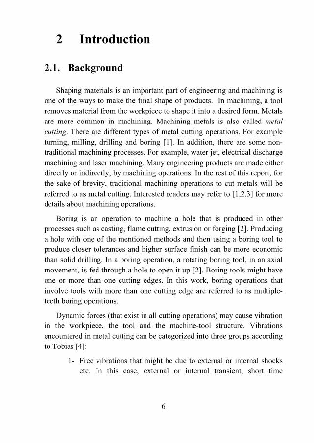
‐ Single-edgon the tooboring too[2].
Figure 4.2
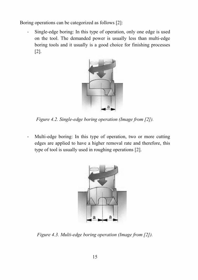
‐ Multi-edgeedges are type of too
Figure 4.
s can be catego
ge boring: In tol. The demanols and it usua
2. Single-edge
e boring: In tapplied to hav
ol is usually us
.3. Multi-edge
15
orized as follow
this type of opnded power isally is a good
e boring opera
this type of opve a higher resed in roughin
boring operat
ws [2]:
peration, only s usually less choice for fin
ation (Image fr
peration, two emoval rate ang operations [2
tion (Image fro
one edge is usthan multi-ed
nishing proces
rom [2]).
or more cuttind therefore, t2].
om [2]).
sed dge ses
ing this

‐ Step-bdiamein ope
F
‐ Reamimulti-
F
The reason foIt is especialldifferent typeMetal Cutting
boring: In thister of the inse
erations [2].
Figure 4.4. Step
ing operation edge tool [2].
Figure 4.5. Re
or using more ly important i
es of boring opg Technical Gu
16
s type of borierts are not eq
p boring opera
is used to pro
eaming operat
than one edgein roughing operations can buide and websi
ng operationqual. This can
ation (Image fr
oduce high pr
tion (Image fro
e in a tool is toperations [2].be found at thite [1,2].
the axial heigimprove chip
from [2]).
recision holes
om [2]).
to boost produ. More details
he Sandvik Co
ght and control
with a
uctivity. s about
oromant

17
Generally, using tools with larger diameters and shortening tool overhang help to reduce vibration in boring operations [2].
4.2. Cutting Forces and Structural Deformations
Figure 4.6 shows a general movement of the head of a boring tool (shown inside a black frame in Figure 4.7) in , and directions due to deformation of the tool.
Other deformations are:
‐ Shrinkage or expansion in the radial direction ‐ Tilting due to bending ‐ Torsion (Twisting around the axis) ‐ Coupled deformations, for example twisting can cause axial
deformation in non-perfect cylindrical shapes. The geometry of boring tools and conditions of the operations cause these deformations to have marginal effects on the regenerative process and therefore they are not considered in the model.
Figure 4.6. , and displacements for the head of a boring tool. Dashed lines represent positions of the insert after one tooth period. The image is generated with the aid of an image file provided by AB Sandvik Coromant.
z
x
y
18
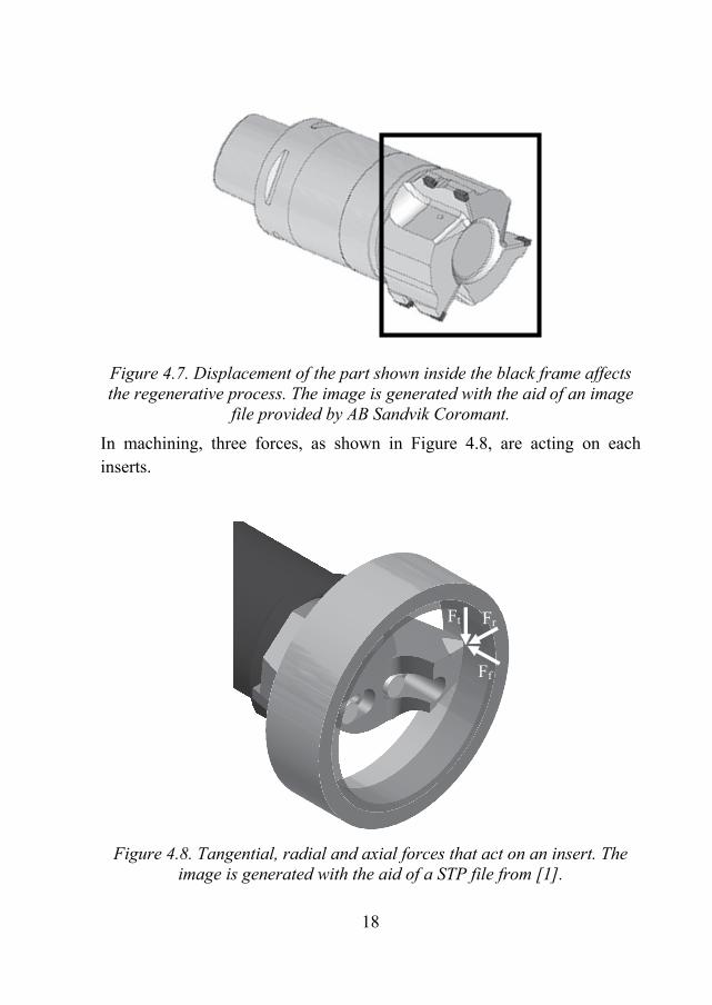
Figure 4.7. Displacement of the part shown inside the black frame affects the regenerative process. The image is generated with the aid of an image
file provided by AB Sandvik Coromant.
In machining, three forces, as shown in Figure 4.8, are acting on each inserts.
Figure 4.8. Tangential, radial and axial forces that act on an insert. The image is generated with the aid of a STP file from [1].
Ff
Fr Ft

19
, and are force components in tangential, radial and feed directions,
respectively. These forces cause deformation of the workpiece, the tool and the machine-tool structure that affect the chip formation. In section 4.3, the chip formation is described in more detail.
4.3. Chip Formation
In boring operations, each insert have axial and rotational movements, simultaneously; therefore, every point on the inserts goes through a helical path during the operation. Figure 4.9 shows the chip formation in a boring operation, when there is no vibration.
Figure 4.9. Insert movement and chip formation in absence of vibrations.
If the forces shown in Figure 4.8 are dynamic, they may cause vibration in , and directions. If there is an axial vibration, it causes wavy surfaces on both sides of the chip as shown in Figure 4.10.
Axial F
eed
Generated chip

20
Figure 4.10. Chip formation when there is a vibration in the axial direction.
The wave shown in Figure 4.10 consists of several cycles. If the number of vibration cycles is an integer in each spindle revolution, the two waves on the chip surfaces are in phase and the thickness of the chip remains constant. On the other hand, if the number of vibration cycles is not an integer number, there is a phase difference and consequently the thickness of the chip changes, as shown in Figure 4.11, and this produces dynamic forces.
Figure 4.11. When the number of cycles in each spindle revolution is an integer (top) and not an integer (down).
Number of cycles in each spindle revolution is an integer
Number of cycles in each spindle revolution is not an integer
Axial F
eed A
xial Feed

21
In boring operation, there is no radial feed. However, this does not mean that dynamic forces are not generated. Figure 4.12 shows what happen if relative displacement between the workpiece and the tool, in the radial direction, is sinusoidal.
Figure 4.12. Chip formation due to radial vibration.
The same as axial vibrations, if the number of vibration cycles, in the radial direction, is not an integer in each spindle revolution, a dynamic chip area is generated as shown in Figure 4.12. Dynamic chip area produces dynamics forces.
In general, vibrations can happen in all three directions simultaneously as shown in Figure 4.13.
x
y Number of cycles in each spindle revolution is an integer
Number of cycles in each spindle revolution is not an integer

22
Figure 4.13. Simultaneous vibrations in , and directions.
When the number of cutting edges is more than one, waves on the chip are generated by successive inserts. In this case, tooth period is used instead of spindle revolution for analyzing. One tooth period is the time that each insert takes to reach the angular position of the previous insert.
4.4. Inserts
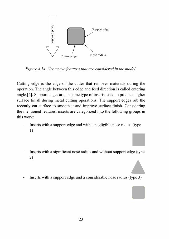
Cutting forces are affected by dynamic chip area. Therefore, stability of the operation is influenced by the chip formation process. In addition to the relative movement between the tool and the workpiece, the geometry of the insert affects the chip formation. Therefore, it is helpful to categorized inserts with respect to their geometry for analysis purposes. Geometric features that affect forces in boring application are cutting edge, entering angle and nose radius [2]. In addition to this features, the support edge can affect generated forces. For more clarity, these features are shown in Figure 4.14.
23
Figure 4.14. Geometric features that are considered in the model.
Cutting edge is the edge of the cutter that removes materials during the operation. The angle between this edge and feed direction is called entering angle [2]. Support edges are, in some type of inserts, used to produce higher surface finish during metal cutting operations. The support edges rub the recently cut surface to smooth it and improve surface finish. Considering the mentioned features, inserts are categorized into the following groups in this work:
‐ Inserts with a support edge and with a negligible nose radius (type 1)
‐ Inserts with a significant nose radius and without support edge (type 2)
‐ Inserts with a support edge and a considerable nose radius (type 3)
Cutting edge Nose radius
Support edge
Axial direction

24
To analyze insert type 3, firstly by the method described in section 5.2, nose radius is incorporated into the depth of cut. By doing this, the insert is simplified into type 1. This means that having the knowledge about analyzing the first two types makes it possible to analyze the last type of inserts. Therefore, only the first two insert types need to be analyzed in detail.
For the first type, see section 5.1, more than one edge are involved in chatter vibrations. It will be shown that the operation can be seen as a combination of turning and milling.
The second type of insert has a more complex geometry. Due to this, an exact approximation of the uncut chip area can be difficult to obtain. A method for calculating the exact uncut chip area of these complex geometries is proposed. This method is then utilized in the time domain stability analysis. For the frequency domain analysis, an additional method for approximating the uncut chip area is presented. This method utilizes polynomial functions to approximate the uncut chip area and greatly reduces the computational time needed.

25
5 Modeling
5.1 Insert Type 1
In this type of insert, the support edge of the insert is parallel to the feed direction, Figure 5.1.
Figure 5.1- An insert type 1
Figure 5.2. A boring tool with inserts of type 1. The image is generated with the aid of an image file from AB Sandvik Coromant.
Radial and axial displacements of an insert after one tooth period are shown in Figure 5.3.

26
Figure 5.3. Radial and axial relative displacements of the insert during one tooth period. Continuous square shows the position of the insert at the present tooth period. Dashed square shows the position of the previous
insert at the previous tooth period.
Both edges of the insert may cut material and generate chips. Therefore, there are two regenerative mechanisms, which can lead to an unstable machining operation. The cutting operation is in the axial direction. As long as the operation is stable, there is no cutting in the radial direction and there is only rubbing. On the other hand, for unstable operations the tool bends and cuts the walls of the hole.
Vibration in the , -plane does not change the uncut chip thickness and therefore does not affect the axial force significantly. On the other hand, vibration in the axial direction causes dynamic forces in axial, tangential and radial directions. The reason is that the axial vibrations change the uncut chip thickness and consequently the chip area. In linear model, cutting forces have a linear relationship with uncut chip thickness [5,19]. Equation ( 5.1) shows the generated force due to vibrations in the axial ( ) direction.
( 5.1)
Axial direction
Radial direction

27
, and are force components in tangential, radial and feed directions,
respectively. , and are cutting force coefficients. Interested reader
may refer to [5,19] for more information about cutting force coefficients. Uncut chip area ( ) is calculated by combining the cutting edge length ( ) and the chip thickness ( ) as follows:
( 5.2)
is obtained by having current positions of the cutter and the workpiece and their positions at the previous tooth period. It is calculated as follows:
h ( 5.3)
and are relative axial positions at the present and previous tooth periods, respectively. Substituting Equation ( 5.2) in Equation ( 5.1) gives:
h
( 5.4)
Force components in , and directions can be obtained from tangential, radial and feed components. Tangential and radial directions rotate as the spindle rotates, on the other hand and directions are fixed in space. is in the axial direction the same as the feed direction. , -plane is perpendicular to the axial direction. The relation between tangential/radial/feed directions and / / directions are given in Equations ( 5.5), ( 5.6) and ( 5.7).
sin cos ( 5.5)
cos sin ( 5.6)
( 5.7)
Substituting Equation ( 5.4) in Equations ( 5.5) - ( 5.7) gives the following relations:
sin cos ( 5.8)
cos sin ( 5.9)

28
( 5.10)
Vibrations in the , -plane produce forces in radial and tangential directions, as shown in Figure 5.4. The assumption is that the tool is turning counterclockwise.
Figure 5.4. Radial and tangential forces due to vibrations in the , -plane. The image is generated with the aid of a STP file from [1].
Numbers 1 and 2 shown in Figure 5.4 indicate two opposite inserts on the boring tool. In vibrations in the , -plane, support edges cut the wall of the hole. Considering the geometry, it can be seen as a milling operation. Therefore, the same formulation as milling for calculating forces can be used. However, the following differences are to be considered:
‐ There are no enter and exit immersion angles.
‐ Radial feed is zero.
‐ The number of the teeth for calculating cutting forces has to be half of all teeth. The reason is that the teeth are analyzed in pairs. This point will be explained later in this section.
x
y
1
2

29
The latter point is valid only for symmetric tools. However, the tool can have either uniform pitch angles or differential pitch angles (for example a tool with four inserts and 100, 80, 100, 80 degrees as pitch angles). In comparison to milling, the second point makes a significant difference in cutting conditions. The radial feed is zero; therefore, if the radial position of the cutter at the present tooth period is smaller than the radial position of the insert at the previous tooth period, the cutter does not cut the workpiece. This effect can make the calculations more difficult. Despite of this fact, in the following part, it is described how to make the calculations simpler.
If insert 1 goes into the workpiece, tangential and radial forces, as shown in Figure 5.4, are calculated as follows:
( 5.11)
( 5.12)
is the dynamic chip area. Dynamic chip area is the part of uncut chip area that changes over the time. It is calculated as follows:
Δ ( 5.13)
is the height of the insert as shown in Figure 5.5. Δ is the difference in the radial immersion after one tooth period.
Figure 5.5. A boring operation with a type 1 insert. is the depth of cut and is height of the insert. The image is generated with the aid of a STP
file from [1].
Axi
s of
the
tool
Axi
al f
eed

30
Difference in the radial immersion is obtained by combining the radial positions of the tool at present and previous tooth periods ( and respectively). Δ is calculated as follows:
Δ ( 5.14)
Δ is a combination of movements in the and directions. The relationship between and its components in the and y directions are as follows:
sin cos ( 5.15)
is the angle between cutting edge and axis and is shown in Figure 5.4.
Therefore, the dynamic chip area is written as follows:
Δ sin Δ cos ( 5.16)
Having the dynamic chip area, Equations ( 5.11) and ( 5.12) are rewritten as follows:
Δ Δxsin LΔ cos ( 5.17)
Δ Δxsin LΔ cos ( 5.18)
Figure 5.6. Generated forces on insert 2. The image is generated with the aid of a STP file from [1].
Fr
Ft
x
y
2
1

31
When insert 1 goes out of the workpiece on one side, insert 2 will simultaneously go into the workpiece on the opposite side of the tool. For a symmetric tool, the distance between insert 1 and the surface of the workpiece is equal to the radial immersion of insert 2. This is due to the assumption of negligible radial shrinkage (or expansion). The forces on insert 2 are shown in Figure 5.6.
Comparison between Figure 5.6 and Figure 5.4 shows that the forces are in opposite directions. Due to symmetry, the forces shown in Figure 5.6 and Figure 5.4 are equal in amplitude. Since the torsion is ignored in the analysis, it is not important where the forces are acting. Therefore, forces that are acting on insert 2 can be assumed to be the same as those acting on insert 1. These forces can be calculated by multiplying a negative sign to Equations ( 5.17) and ( 5.18). This negative sign multiplication can be interpreted as a negative area that is produced by a negative Δr. Despite of the fact that there is no negative area, this new concept helps to use the same formulas for describing of generated forces in inserts moving both into and out of the workpiece. The only consideration is that the total force on the tool has to be calculated for half of the inserts because the inserts are used in pairs. Combining Equations ( 5.5), ( 5.6), ( 5.17) and Equation ( 5.18) gives Equation ( 5.19) which describes the relationship between generated dynamic forces in and directions and displacements in these directions due to vibrations in the , -plane (for more details see [5]).
12
ΔΔ
( 5.19)
Equations ( 5.20) - ( 5.23) show the values of , , and [5].
g sin 2 1 cos 2 ( 5.20)
g 1 cos 2 sin 2 ( 5.21)

32
g 1 cos 2 sin 2 ( 5.22)
g sin 2 1 cos 2 ( 5.23)
is the number of cutting edges (inserts) on the tool. g is a function that
is 0 whenever the cutting edge is not inside the workpiece due to the effects of tool jumping out of cut and enter/exit angles. g is 1 otherwise [5]. is
the height of the insert as shown in Figure 5.5. It can be seen as the depth of cut for support edge of the insert.
Now adding forces that are produced by vibrations in both the direction and the , -plane, gives:
ΔΔΔ
( 5.24)
Matrix is calculated as follows:
12
12
sin cos
12
12
cos sin
0 0
( 5.25)
Equation ( 5.24) shows the generated forces for all inserts. Equations ( 5.24) and ( 5.25) can be used directly in the time domain simulation.
5.1.1 Time domain simulation
In the time domain, the governing equations for the dynamic system are presented by a system of differential equations (if the number of masses is more than one). Numerical methods can be used to solve this system of equations. In order to trigger the regenerative vibrations, a small disturbance of the system is needed. A small impulse can be used as an initial disturbance. If the response of the system becomes smaller in

33
magnitude over time, the operation is stable. On the other hand, if the response grows exponentially, the operation is unstable.
Figure 5.7. Block diagram in MATLAB SIMULINK® for the time domain simulation of a boring operation.
dx
dy
To
Wor
kspa
ce3
delta
z
To
Wor
kspa
ce1
delta
y
To
Wor
kspa
ce
delta
xSe
tting
s
−C−
Initi
al d
istu
rban
ce
G_z
z
num
z(s)
denz
(s)
G_y
y
num
y(s)
deny
(s)
G_x
x
num
x(s)
denx
(s)
Feed
−K−
Em
bedd
edM
AT
LA
B F
unct
ion
setti
ng1
phi_
j
x x0 y y0 z z0
Fx Fy Fz
Forc
eCal
cula
tor
Del
ay2 D
elay
1
Del
ay
Clo
ck0

34
In this thesis, MATLAB SIMULINK® is used to solve the governing equations in the time domain. MATLAB SIMULINK® allows representing a system by its transfer function. Delay blocks are added to the model in order to represent the time delays between teeth. The length of the simulated response has to be long enough to make a correct decision about the stability. The time step for the time domain analysis determines the sampling frequency for the input signal and consequently it is important to meet the sampling theorem criterion.
Figure 5.7 shows the block diagram for the time domain simulation of a boring operation with multiple-teeth boring tool. The block of ForceCalculator calculates the forces and its settings are dependent on the type of insert.
In the time domain analysis, the changes in time response determine whether the operation is stable or not. In an unstable operation the amplitude of the signal (can be displacement or force) grows exponentially. As an example, Figure 5.8 shows displacement signals for an unstable operation.
Figure 5.8. Simulation output for an unstable operation.
0 0.1 0.2 0.3 0.4 0.5 0.6 0.7 0.8−1
−0.5
0
0.5
1x 10
−6
x [m
]
0 0.1 0.2 0.3 0.4 0.5 0.6 0.7 0.8−1.5
−1
−0.5
0
0.5
1
1.5x 10
−6
Time [sec]
y [m
]

35
5.1.2 Frequency Domain Simulation
Equation ( 5.25) cannot be used in the frequency domain analysis because the angular positions of the inserts are time dependent and consequently is time dependent. Since elements of are periodic
with period of Δ , Fourier series can be used [5]. In milling
operations, the average value in Fourier series gives good approximation [7]. Here, for boring, the same assumption is made:
1Δ
( 5.26)
Substituting Equation ( 5.25) in ( 5.26) gives:
00
0 0
( 5.27)
Values of , and , after integration, are as follows:
14
( 5.28)
14
( 5.29)
14
( 5.30)
14
( 5.31)
Using matrix instead of in Equation ( 5.24) gives:
00
0 0
ΔΔyΔ
( 5.32)
In Equation ( 5.32), radial and axial directions are decoupled. Considering the geometry, it can be said that the stability analysis in the axial direction is the same as turning and in the radial direction is the same as milling.

36
Therefore, the milling analysis is needed. The following part shows the method presented in [5,7] for stability prediction of milling operations.
In the , -plane the forces are:
ΔΔy
( 5.33)
The transfer function for the tool is written as follows:
( 5.34)
The relationship between input force and output displacement for the tool is:
F ( 5.35)
Equation ( 5.35) means that if the input is harmonic, the response is harmonic with the same frequency but different phase and amplitude. The differences in phases and amplitudes are determined by . For the previous tooth period, displacement is as follows:
( 5.36)
is the time delay for each tooth periods. Now the displacement after one tooth period can be obtained as follows:
ΔΔ 1 F
( 5.37)
Equation ( 5.37) shows the displacement during one tooth period when the input is a sinusoidal force with the frequency of .
Substituting ( 5.37) in ( 5.33) gives the following relation:
1
( 5.38)
Equation ( 5.38) can be rewritten as follows

37
( 5.39)
( 5.40)
1 ( 5.41)
Equation ( 5.39) is an eigenvalue problem. In the left hand side, there is a vector and on the right hand side of the equation, the same vector is multiplied with a square matrix. To have the answer for this problem, Equation ( 5.42) should be solved:
1 0 ( 5.42)
Equation ( 5.42) can be rewritten as follows:
Λ 0 ( 5.43)
Λ is the eigenvalue of the problem. 0 and Λ are calculated are as follows:
( 5.44)
Λ L 1cos sin
( 5.45)
In many practical milling cases, the cross transfer functions are negligible [16] .If the cross transfer functions are zeros, becomes:
( 5.46)
Equation ( 5.43) can be solved analytically. The characteristic equation is as follows:
1 0 ( 5.47)
The coefficients of this quadratic equation are as follows:
( 5.48)

38
( 5.49)
Generally, the eigenvalue is a complex number. Therefore, it has a real and an imaginary part:
Λ Λ Λ ( 5.50)
is real part of the eigenvalue and is imaginary part of it.
Comparing ( 5.50) and ( 5.45) gives:
1 cos ( 5.51)
sin ( 5.52)
Now new variables κ and are introduced as follows:
κ tansin
1 coscot
2
tan2 2
( 5.53)
Substituting κ in real part of the eigenvalue gives:
1 cos 2 sin2
2
1 cot
21
( 5.54)
Rearranging ( 5.54) gives the height limit for chatter vibrations as follows:
12
( 5.55)
This means that if the height of the insert is less than , the operation is stable and for values bigger than this limit, the operation is unstable.
Now it is important to find the corresponding spindle speed for each height limit. For any given frequency, there is an eigenvalue that can be obtained from ( 5.43). In each frequency, there is a phase difference between waves on each sides of the chip and this phase difference is obtained from the following equation:
ϵ π 2 ( 5.56)

39
There is a time delay corresponding to each phase difference that can be obtained from following equation:
ωcT ϵ 2kπ ( 5.57)
Therefore, the time delay is calculated as follows:
T1
ωcϵ 2kπ
( 5.58)
Having the time delay, the spindle speed is obtained as follows:
60
T ( 5.59)
The unit for spindle speed is revolutions per minute rpm .
In the same way, it is possible to do stability analysis for the axial direction by solving following eigenvalue problem:
1 ( 5.60)
is the transfer function in direction. The chatter limit and spindle speed are calculated similar to previous part.
Λ 1 1 cos sin ( 5.61)
Λ is the eigenvalue for Equation ( 5.60).
κ tansin
1 cos
( 5.62)
ΛR 1 cos21
( 5.63)
bΛR
21
( 5.64)
is radial immersion of the tool. Equations ( 5.56)-( 5.59) can be used to calculate spindle speed.
Cutting edge contact length ( ) affects cutting forces [11]. generates a force that is constant in value if the length of the contact is not changing during the operation. In vibrations in the , -plane, for the current type of insert, the cutting edge contact length remains constant when the insert

40
have a radial immersion and it is zero when the tool is not inside the workpiece. Therefore, the generated force is in the form of square wave as shown in Figure 5.9.
Figure 5.9. The force due to cutting edge contact length . The numbers in the graph are not valid; the graph only shows that the force is a square
wave.
This force is periodic and therefore it can be decomposed into harmonics. Since the amplitude of the square wave does not change, the amplitudes of the harmonics do not change. This means that they do not have any contribution to the regenerative process and this means that for this type of insert the cutting edge contact length does not affect the stability in the , -plane.
It is worth mentioning that height of the insert has two effects:
1- Affecting the uncut chip area and consequently affecting the forces. 2- Affecting the forces values, directly.
The latter is not used for chatter vibrations analysis, because it does not affect the regenerative process as mentioned above. On the other hand, area has a dynamic change during the process. Therefore, there is a limitation for height of the insert due to its contribution to the uncut chip area. This means that height of the insert affect the regenerative process due to its indirect effect on cutting forces. To avoid mixing up, two different
0 1 2 3 4 5 6 7 80
2
4
6
8
10
Time
Forc
e

41
symbols are used for height of the insert. refers to the height of the insert when its direct effect is considered and refers to the height of the insert when it is used for the uncut chip area calculation.
5.1.3 Simulation in the Time and Frequency Domains
In this section, the results of the time domain and the frequency domain simulations for an insert of type 1 are shown. Figure 5.10 and Figure 5.11 show the chatter limits for a given tool with 3 inserts of type 1. Modal parameters of this tool are listed in Table 5.1.
Figure 5.10. Chatter limits for height of the insert. Triangles and dots are for stable and unstable operations, respectively (the time domain
simulation). Solid lines are results of the frequency domain simulation.
500 550 600 650 700 750 800 850 900 950 10000
0.005
0.01
0.015
Spindle speed [rpm]
Hei
ght o
f in
sert
[m
]

42
Table 5.1 Modal parameters of a given tool with three insert of type 1.
Pole Residue ( 10 )
-18.485+j909.05 -157.47+j4183.2 -j0.28763 -j1.2816
-44.928+j975.69 -69.909 +j1962.1 -j0.29313 -j0.22308
-32.025+j1585.1 j0.040739
In Figure 5.10 and Figure 5.11, the time domain results are shown in dots and triangles and the frequency domain results are shown in solid lines. Triangles represent stable operations and dots are for unstable operations. Since there are two edges, there are two analyses. Figure 5.10 shows the chatter limit prediction for support edge that means the stability diagram shows the chatter limits for the height of the insert. The simulations parameters are listed in Table 5.2.
Table 5.2. Simulation parameters that are used for producing Figure 5.10.
Depth of cut ( ) 0.5 mm
Sampling frequency in the time simulation 10000 Hz
Number of cutting edges 3
Entering angle 90 degrees
Type of the insert Type 1
0.2 mm/tooth
1300 N/mm
800 N/mm
As shown in Figure 5.10, for large height of insert the operation is completely unstable for all spindle speeds.

43
For the cutting edge, the stability analysis is achieved using Equations ( 5.56)-( 5.64). The results are shown in Figure 5.11. The simulation parameters are listed in Table 5.3.
Figure 5.11. Chatter limits of the depth of cut. Triangles and dots are for stable and unstable operations, respectively (the time domain simulation).
Solid lines are results of the frequency domain simulation.
Table 5.3. Simulation parameters that are used for producing Figure 5.11.
Height of the insert ( ) 7 mm
Sampling frequency in the time simulation 10000 Hz
Number of cutting edges 3
Entering angle 90 degrees
Type of the insert Type 1
0.2 mm/tooth
1300 N/mm
800 N/mm
500 550 600 650 700 750 800 850 900 950 10000
0.01
0.02
0.03
0.04
0.05
0.06
0.07
0.08
0.09
0.1
Spindle speed [rpm]
Dep
th o
f cu
t [m
m]

44
As shown in Figure 5.11, there are some regions that stability analysis in the time domain shows them as unstable points (dots) while in the frequency domain they look stable, for example for spindle speed of 800 rpm . In fact, such points are unstable as shown in the time domain analysis. For the frequency domain analysis, it is necessary to look at Figure 5.10 and Figure 5.11 together. For example for spindle speed of 800 rpm , Figure 5.10 shows it as an unstable point for height of 7 mm .
As shown in Figure 5.10 and Figure 5.11, the frequency domain results match the time domain results. This means that despite of simplifications in the frequency domain analysis, the frequency domain approach still provides accurate results. In addition, the suggested method for modeling the insert jumping out of cut, in the frequency domain, works well.
5.2 Insert Type 2
Figure 5.12. An insert of type 2 on a boring tool. Image is produced with the aid of a STP file from [1].
An insert of type 2, Figure 5.12, have a significant nose radius and it does not have support edge. For inserts of this type, the analysis is more complicated compared to inserts of type 1 due to the geometry differences between these insert types. Figure 5.13 shows the displacement of the insert after one tooth period.

45
Figure 5.13. Displacement of the insert during one tooth period.
Gray area shows the uncut chip area. The area of the uncut chip affects the generated forces. Vibrations in radial and axial directions influence this area. Using the geometric relations, the area of the chip is found and it can be used in the time domain analysis directly. In the time domain, the positions of the cutting edges are calculated in each time step. Having these positions, it is possible calculate the exact uncut chip area in each time step and use it in the time domain simulation. On the other hand, the exact area is too complex to be used in the frequency domain analysis. In the frequency domain analysis, positions of the inserts are not calculated in every time step, and it is needed to have a time-independent linear relationship between dynamic forces and infinitesimal changes in , and directions ( , and ). Therefore, a simpler formula for calculating
the uncut chip area is essential.
In the following sections, first, the exact uncut chip area is calculated. After that, a method is proposed for approximating this area in order to be used in the frequency domain analysis.
The calculation is done for the insert with product code of CCMT 06 02 08-PM 4235. The specifications of this insert are given in Figure 5.14.
Axi
al f
eed
dire
ctio
n

Figure 5.14.
5.2.1 Ex
Figuresupport edge is bigger than[11]).
Figur
. An insert of tytable
xact Area Cal
e 5.15 shows thand with nose
n the feed rate
re 5.15. Gener
Axial f
Wall of the pr
46
type 2 that is ue and figures a
lculation
he generated ce radius). The e per tooth (tha
rated chip for a
feed direction
re-bored hole
used for analysare from [1].
chip by an inseassumption is
at is common
a tool with ins
sis in this work
ert of type 2 (ws that the nosein boring ope
sert of type 2.
Entering an
Nose r
k. The
without e radius erations
ngle
radius

Twoand desclittlenot
To cas sh
a h
direradiSincknownoseis lobefo
Havexac
o cases might second the de
cribes the waye different. Hodescribed in th
calculate the ehown in Figur
Figure 5
and are the has the coord
ection. is dial vibration (vce the coordinwn, can bee radius and ceocated on the lore boring.
ving the above ctly calculated
happen, first epth of cut is sy of area calcuowever, the gehis report.
exact uncut chire 5.16.
5.16. Splitting u
centers of thedinates of due to the axiavibration in thnates of the cee found. andenters of the cline of .
points, the ared:
47
the depth of csmaller than nlation for the feneral approac
ip area, the are
up the total ar
e nose circles. in the axial d
al feed and axhe , -plane).enters of the cd can be fo
circles. has t and are l
eas shown in F
Feed
dr
cut is bigger tnose radius. Thfirst case. Thech is the same
ea is split up i
rea into smalle
is assumeddirection and xial vibration. is located
circles and theound by havingthe radial coorlocated on the
Figure 5.17 to
E
than nose radihe following pe second case ie. Therefore, it
into smaller pa
er parts.
d to be the orig in the rad is due to
d on both circle nose radius g entering angrdinate as a
e wall of the h
Figure 5.22 ar
Entering angle
Nose radiu
ius, part is a t is
arts
gin. dial the les. are
gle, and ole
re
e
us
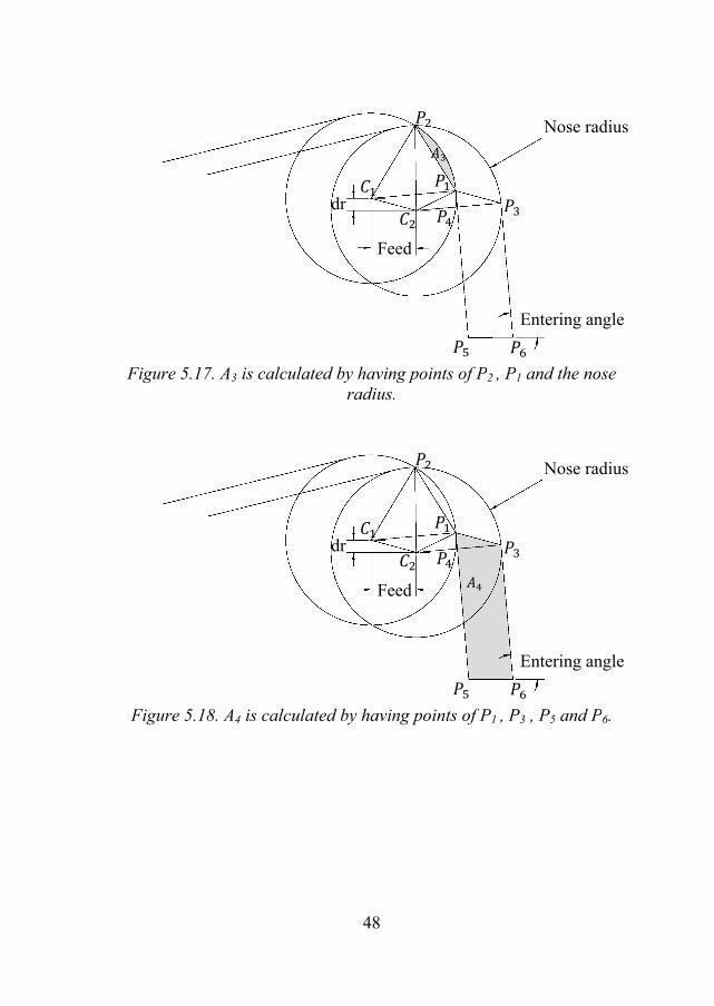
Figure 5.1
Figure 5.
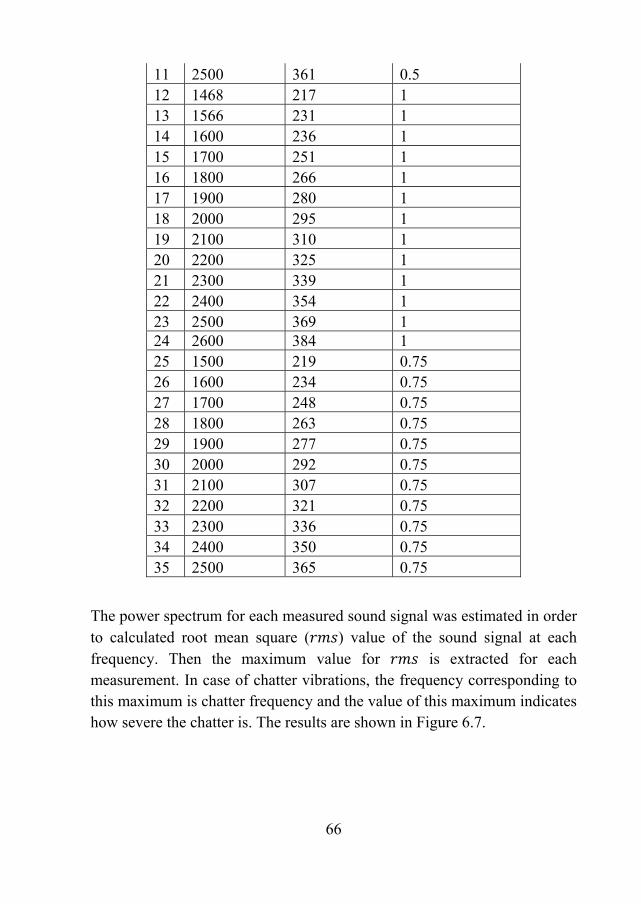
17. A3 is calcu
18. A4 is calcu
48
ulated by havinradius.
ulated by havin
Fe
dr
Fe
dr
ng points of P2
.
ng points of P1
eed
eed
, P1 and the n
1 , P3 , P5 and P
Entering a
Nose r
Entering a
Nose r
nose
P6.
angle
adius
angle
adius

Figure 5.19.
Figure 5.20.
. Atr1 is calcula
Atr2 is calcula
49
ated by having
ated by having
Feed
dr
Feed
dr
g points of P1 ,
g points of P1 ,
E
E
P2 and C2.
P3 and C2.
Entering angle
Nose radiu
Entering angle
Nose radiu
e
us
e
us

Figu
The area of th
is the total a
Figure 5.21. A
ure 5.22. A2 is c
he uncut chip i
area of uncut c
50
As is the area o
calculated by
is calculated as
chip.
Fe
dr
Fe
dr
of the section P
having ,
s follows,
eed
eed
P2P3C2.
, , .
( 5
Entering a
Nose r
Entering a
Nose r
5.65)
angle
adius
angle
adius

51
( 5.66)
5.2.2 Area Approximation
The exact area, calculated in section 5.2.1, can be used in the time domain to obtain stability diagrams. However, it cannot be used in the frequency domain analysis, due to its complexity. Therefore, a good approximation for it is essential.
In the first place, it is assumed that the uncut chip area is a function of depth of cut, radial and axial displacements during one tooth period.
, , ( 5.67)
: Uncut chip area
: Depth of cut
: Radial displacement during one tooth period due to radial vibration
: Axial displacement during one tooth period (feed plus axial vibration).
It is intended to have a linear relationship between cutting forces and infinitesimal changes in , and directions ( , and ). It is assumed that cutting forces are linearly related to the uncut chip area, therefore a linear relationship between , and and uncut chip area is sought. A suggestion for the uncut chip area is as follows:
( 5.68)
, and are unknown functions of and they must be found.
Putting 0 in Equation ( 5.68) gives:
( 5.69)
Assuming 0 and plotting the area versus for different , gives the
plot shown in Figure 5.23.

52
Figure 5.23. Uncut chip area versus depth of cut ( ) for different . Assumption is that 0.
Figure 5.23 shows a linear relationship between the area and depth of cut and it is observed that:
( 5.70)
This means that and is very small compared to .
Now it is assumed is not zero and that is a value between 10 and 10 m . To calculate and , is subtracted from the total
uncut area ( ) that gives:
( 5.71)
is the remaining area after subtraction of . Figure 5.24 shows the
remaining area ( ) versus depth of cut ( ) for different values of .
0.2 0.4 0.6 0.8 1 1.2 1.4 1.6 1.8 2
x 10−3
0
0.2
0.4
0.6
0.8
1
1.2
1.4
1.6
1.8
2x 10
−7
ap [m]
A [m
2 ]

53
Figure 5.24. Remaining area ( ) versus depth of cut ( ) for different values of (for between 10 and 10 ).
Despite of the fact that the remaining area is small compared to , it has
a significant effect on the stability of the operation. Polynomial functions can be used as approximations for the remaining area. It is difficult to fit one polynomial function to the whole curve. Therefore, more than one function is needed to capture the curve correctly.
The range of the depth of cut is split up into smaller parts as follows:
‐ Part 1: 0.01 mm 0.2 mm
‐ Part 2: 0.2 mm 0.7 mm
‐ Part 3: 0.7 mm 2 mm
Figure 5.25 to Figure 5.27 shows for above ranges of .
0.2 0.4 0.6 0.8 1 1.2 1.4 1.6 1.8 2
x 10−3
−1.1
−1
−0.9
−0.8
−0.7
−0.6
−0.5
−0.4
−0.3
−0.2
−0.1
x 10−10
ap [m]
Ar [m
2 ]

54
Figure 5.25. for range of part 1.
Figure 5.26. for range of part 2.
0.2 0.4 0.6 0.8 1 1.2 1.4 1.6 1.8 2
x 10−4
−9
−8
−7
−6
−5
−4
−3
−2
−1x 10
−11
ap [m]
Ar [m
2 ]
2 3 4 5 6 7
x 10−4
−1
−0.9
−0.8
−0.7
−0.6
−0.5
−0.4
−0.3
−0.2
−0.1
0x 10
−10
ap [m]
Ar [m
2 ]

55
Figure 5.27. for range of part 3.
For part 1 and part 2, quadratic polynomials are used to approximate and . For part 3, a linear approximation is accurate enough.
The following equation shows the approximation for the remaining area, :
( 5.72)
Therefore, the total area becomes:
( 5.73)
Coefficients p to p are calculated separately for each part.
If a is assumed to be constant during the operation and if the tool is very
rigid in the axial direction, the dynamic area is calculated as follows:
( 5.74)
Assuming:
0.8 1 1.2 1.4 1.6 1.8 2
x 10−3
−1.1
−1
−0.9
−0.8
−0.7
−0.6
−0.5
−0.4
−0.3
−0.2
−0.1
x 10−10
ap [m]
Ar [m
2 ]

56
( 5.75)
Then:
( 5.76)
If Equation ( 5.76) and Equation ( 5.13) are compared, it is seen that they are the same if , now using Equations ( 5.11) to ( 5.59) it is possible to calculate the chatter limits for multiple-teeth boring tools with insert of type 2. After calculating C, Equation ( 5.75) is used to calculate the depth of cut (a ).
5.2.3 Simulations in the Time and Frequency Domains
In this study the for time domain simulation, the exact area is calculated as described in section 5.2.1 and MATLAB SIMULINK® is used for implementing. For frequency domain simulation, area is approximated by method presented in section 5.2.2.
Figure 5.28. Chatter limits for depth of cut for a tool with three inserts as shown in Figure 5.14. Triangles and dots are for stable and unstable operations, respectively (the time domain simulation). Solid lines are
results of the frequency domain simulation.
1000 1100 1200 1300 1400 1500 1600 1700 1800 1900 2000 2100 2200 2300 2400 25000
0.2
0.4
0.6
0.8
1
1.2
1.4
1.6
1.8
2x 10
−3
spindle speed [rpm]
Dep
th o
f the
cut
[m]

57
Figure 5.28 shows the stability analysis results in the time and frequency domains for a tool with three inserts with specifications given in Figure 5.14 and entering angle of 95 degrees.
It can be seen that the time domain and the frequency domain analysis match up. This means that the proposed method for area approximation gives acceptable results. The frequency domain analysis is done by approximating the uncut chip area. Therefore, the frequency domain simulation is valid only in the range that the area is approximated. In the current case, the approximation is for 0.01 mm up to 2 mm .
For high depths of cut, instability in axial direction becomes more dominant and in the gaps in Figure 5.28, the operation becomes axially unstable.

58
6 Experimental Results
To validate the theory it is needed to see whether the stability diagram correlates with experimental data. First step is identification of the dynamic system. After that, the cutting force coefficients are measured and finally sound pressures at several points are measured. In these experiments, a rigid workpiece is used and therefore the combination of tool and machine-tool is assumed as the flexible part of the system. In this chapter, a set of experiments is done for a tool with three inserts as shown in Figure 5.14.
6.1 FRF Measurements (System Identification)
In structural dynamics, a transfer function represents a dynamic system [20]. However, transfer functions cannot be measured directly [20]. To obtain the transfer function of a system, frequency response function (FRF) of the system is measured [20]. After that, using experimental modal analysis techniques, modal parameters are extracted. Having modal parameters of a system, the transfer function in the Laplace domain (s-plane) is obtained [20]. Modal analysis methods are given in detail in [18,20]. Figure 6.1 shows the frequency response functions for and directions that are obtained experimentally. The dominant frequency is around 500 for both and . Therefore, only this frequency is used in the analysis. Table 6.1- Extracted poles and residues for the given tool.
Pole Residue ( 10 )
direction 76.152 +j3591.03 0.29553-j3.2065
direction 75.398 +j3555.4 0.62879 -j6.8224

59
Figure 6.1. Experimental FRFs in and directions.
Figure 6.2. Synthesized frequency response functions for and directions.
0 1000 2000 3000 4000 50000
0.2
0.4
0.6
0.8
1x 10
−6
Frequency [Hz]
Dyn
amic
fle
xibi
lty [
m/N
]
FRF
x
FRFy
0 1000 2000 3000 4000 50000
0.2
0.4
0.6
0.8
1x 10
−6
Frequency [Hz]
Dyn
amic
fle
xibi
lty [
m/N
]
FRF
x
FRFy

6.2 M
In thisgiven in sectiocutting edge cmeasure cuttinuncut chip arerate per tooth.shown in Tab
Figure
Table 6.2 shomeasurement.
Measuring
s section, cuttinon 5.2. Cuttingcontact length ng force coeffeas. Uncut chi. Therefore, dile 6.2) to have
e 6.3. Experim
ws the spindle.
60
Cutting F
ng force coeffg forces are rethrough cuttin
ficients, forcesip area is depeifferent depthse different chip
mental set up fo
e speed, feed r
orce Coeff
ficients are calclated to uncut
ng force coeffi are to be mea
endent on depts of cut and feep areas.
or measuring c
ate and depth
ficients
culated for thechip area, andcients [11]. To
asured for diffeth of cut and feed rates are use
cutting forces.
of cut for each
e tool d o erent eed ed (as
h

61
Table 6.2. Depth of cut and feed rate for each measurement.
No. Feed mm mmFinal hole diameter mm
Spindle speed rpm
1 0.05 0.5 46 1834 2 0.075 0.5 46 1834 3 0.1 0.5 46 1834 4 0.125 0.5 46 1834 5 0.15 0.5 46 1834 6 0.05 0.75 46.5 1834 7 0.075 0.75 46.5 1834 8 0.1 0.75 46.5 1834 9 0.125 0.75 46.5 1834
10 0.15 0.75 46.5 1834 11 0.05 1 47 1795 12 0.075 1 47 1795 13 0.1 1 47 1795 14 0.125 1 47 1795 15 0.15 1 47 1795 16 0.05 1.25 47.5 1776 17 0.075 1.25 47.5 1776 18 0.1 1.25 47.5 1776 19 0.125 1.25 47.5 1776 20 0.15 1.25 47.5 1776 21 0.05 1.5 48 1757 22 0.075 1.5 48 1757 23 0.1 1.5 48 1757 24 0.125 1.5 48 1757 25 0.15 1.5 48 1757 26 0.05 2 49 1721 27 0.075 2 49 1721 28 0.1 2 49 1721 29 0.125 2 49 1721 30 0.15 2 49 1721

62
By method explained in section 5.2.1, exact area in each case is calculated. Forces are measured in , and directions using a dynamometer. The experimental setup is shown in Figure 6.3.The measured forces are periodic and their period is the same as the spindle period. Since the conditions for the cutting operation remain unchanged during the operation, it is concluded that the total force remains constant. If the force in the axial direction remains constant during the operation, the force in the , -plane also remain constant. Knowing this fact, the total force in the , -plane is calculated for each case as follows:
( 6.1)
Figure 6.4 shows the force components for a cutting depth, 0.5 mm
and feed rate, 0.075 mm/tooth].
Figure 6.4. Force component in , and directions, for depth of cut of 0.5 and feed rate of 0.075 / .
0 0.1 0.2 0.3 0.4 0.5 0.6 0.7−250
−200
−150
−100
−50
0
50
100
150
200
250
Forc
e [N
]
Time [sec]
F
x
Fy
Fz

63
As shown in Figure 6.4, and components of the force are periodic due to the tool rotation. Using Equation ( 6.1) the total force in the , -plane is calculated. The result is shown in Figure 6.5.
Figure 6.5. Force in the , -plane, for depth of cut of 0.5 and feed rate of 0.075 / .
As shown in Figure 6.5 the total force in the , -plane is a fluctuating value around 190 N in this case. The average of this value is calculated for using in the model. Doing this calculation for all cases in Table 6.2 and plotting the result versus uncut chip area makes it possible to find a relationship between the force and the uncut chip area. This plot is shown in Figure 6.6.
0 0.1 0.2 0.3 0.4 0.5 0.6 0.70
50
100
150
200
250
Tot
al f
orce
[N
]
Time [sec]
Force in xy−plancemean value

64
Figure 6.6. Total force in the , -plane versus uncut chip area.
As shown in Figure 6.6 the relationship between force and area is linear. This line has a small offset from the origin that is mainly due to the cutting edge contact length ( ). The relationship between the total force in the , -plane and the uncut chip area is as follows:
( 6.2)
is uncut chip area. and are as follows:
2.2933 10 N , 111.5225 N
is mainly due to cutting edge contact length and it is ignored in the model because of its small value. From the total force in the , -plane, the tangential and radial components are calculated as follows:
cos ( 6.3)
0 0.5 1 1.5 2 2.5
x 10−7
150
200
250
300
350
400
450
500
550
600
650
Area [m2]
Tot
al f
orce
in x
y−pl
ane
[N]
Total force in xy−planeLinear regression

65
sin ( 6.4)
is the angle between and tangential direction. and are tangential
and radial components, respectively. Equations ( 6.3) and ( 6.4) give:
tan ( 6.5)
Since is bigger than , is a value between 0 to 45 degrees depending on cutting conditions. Equations ( 6.6) and ( 6.7) are used to calculate cutting force coefficients.
cos ( 6.6)
sin ( 6.7)
6.3 Measuring the Sound of Vibrations (Model Verification)
For the given tool, sound levels during operations are measured for different cutting conditions. These cutting conditions are shown in Table 6.3.
Table 6.3. Cutting conditions for measured sounds of cutting operations.
No. Spindle speed rpm
cutting speed m/min
Depth of cut mm
1 1500 217 0.5 2 1600 231 0.5 3 1700 245 0.5 4 1800 260 0.5 5 1900 274 0.5 6 2000 289 0.5 7 2100 303 0.5 8 2200 318 0.5 9 2300 332 0.5 10 2400 347 0.5
66
11 2500 361 0.5 12 1468 217 1 13 1566 231 1 14 1600 236 1 15 1700 251 1 16 1800 266 1 17 1900 280 1 18 2000 295 1 19 2100 310 1 20 2200 325 1 21 2300 339 1 22 2400 354 1 23 2500 369 1 24 2600 384 1 25 1500 219 0.75 26 1600 234 0.75 27 1700 248 0.75 28 1800 263 0.75 29 1900 277 0.75 30 2000 292 0.75 31 2100 307 0.75 32 2200 321 0.75 33 2300 336 0.75 34 2400 350 0.75 35 2500 365 0.75
The power spectrum for each measured sound signal was estimated in order to calculated root mean square ( ) value of the sound signal at each frequency. Then the maximum value for is extracted for each measurement. In case of chatter vibrations, the frequency corresponding to this maximum is chatter frequency and the value of this maximum indicates how severe the chatter is. The results are shown in Figure 6.7.

67
Figure 6.7. Maximum sound pressure level for each cutting condition.
Experimental data shown in Figure 6.7 indicate that for spindle speeds around 1600, 1900 and 2250 rpm the vibration level is significantly lower. Looking at measured sound at time domain showed that there is no chatter in the region mentioned above. Comparing the obtained experimental data with simulation results, shown in Figure 6.8, shows that experimental data validate the simulation results.
In Figure 6.8, dots and triangles represent unstable and stable points respectively that are resulted from the time domain simulation. Continuous lines show the thresholds of stability, obtained from the frequency domain analysis. Photo on the top of the plot shows the surface finish for two different boring conditions. Specifications of the tool are given in section 5.2. Depth of cut for both cases are 0.5 . In spindle speed of 1500
, the operation is unstable and in 1900 it is stable according to simulation results (both in frequency and time domains). As shown in the photo, experimental results validate the simulation results.
1400 1600 1800 2000 2200 2400 260045
50
55
60
65
70
Spindle speed [rpm]
dBSP
L
depth of the cut=0.5depth of the cut=0.75depth of the cut=1

Figure 6
10000
0.2
0.4
0.6
0.8
1
1.2
1.4
1.6
1.8
2x 1
Dep
th o
f the
cut
[m]
6.8. Chatter lispecificat
1100 1200 1300 1400
0−3
68
mits for a tooltions are given
0 1500 1600 1700 180spindle speed
l with three insn in Figure 5.1
00 1900 2000 2100 22[rpm]
serts (the inser14).
200 2300 2400 2500
rt

69
7 Variable Pitch Angles
Variable pitch angles can be used in order to increase the stability in metal cutting operations [16]. Variable pitch angles hinder regenerative processes and therefore increase the stability [16]. In the time domain analysis, general approach is the same as uniform pitch angle. However, to implement variable pitch angles in the time domain, different time delays for each inserts are needed. The amount of delays are determined by pitch angles and speeds of the spindle. As it was discussed in chapter 5, it is possible to use approaches for milling operation to analyze boring operations. Therefore, the method for analyzing nonconstant pitch angles in milling can be employed for the boring as well. An analytical design method to increase the stability for milling cutters with variable pitch angles is presented in [16,17]. This method is described in the following part.
In the frequency domain analysis, the approach is a little different from what was explained for constant pitch angles. In this case, Equation ( 5.45) cannot be used because the pitch angles are not the same for all inserts, this means that:
Λ L 1
cos sin
( 7.1)
and are introduced as follows:
cos ( 7.2)
sin ( 7.3)
Substituting Equations ( 7.2) and ( 7.3) in Equation ( 7.1) gives:

70
Λ ( 7.4)
Rearranging Equation ( 7.4) gives the chatter limit in terms of as follows:
LlimΛ
( 7.5)
The limit obtained from Equation ( 7.5) has an imaginary part and a real part. However, this limit should be a real number that means the imaginary part has to be zero. This means that to find the chatter limits it is necessary to find the zeros of imaginary part and then having the corresponding frequency, the chatter limits are found. The difference with the case of constant pitch angle is that here an explicit formula such as Equation ( 5.55) is not available.
Figure 7.1 shows the stability lobes for the boring tool given in section 5.2 and with variable pitch angles. The pitch angles are 108, 108 and 144 degrees.
Figure 7.1. Stability lobes for the tool given in section 5.2. Pitch angles are 108,108 and 144 degrees.
The same approach can be used for tools with inserts of type 1.
1000 1500 2000 25000
0.2
0.4
0.6
0.8
1
1.2
1.4
1.6
1.8
2x 10
−3
spindle speed [rpm]
Dep
th o
f cu
t (a p)
[m]

71
8 Discussion and Conclusion
Stability analysis in multiple-teeth boring operations were investigated in this thesis. The aim was to find an accurate, easy to implement and fast simulating model to analyze chatter vibrations.
Different methods were proposed for different types of tools. Different inserts were categorized based on the insert shape. In each case, simulations were done both in the time domain and in the frequency domain and were shown that the simulation results in both domains agree with each other. Since the cutting forces are affected by uncut chip area, different methods to calculate uncut chip area were proposed. When the uncut chip has a complex geometry, it is difficult to use the exact area calculation in the frequency domain. A method which approximates the uncut chip area by the aid of polynomial functions was therefore proposed. Comparisons between time domain and frequency domain simulations show good agreement and the simplifications made in the frequency domain analysis do not have a significant effect on the simulation results. Experimental tests were also conducted for one of the studied tools. The experimental results agreed with simulation results obtained by the proposed models. By using the stability diagrams as described in Chapter 5, it is possible to investigate whether the operation is stable or not, for a given set of cutting data. The effects the tool and workpiece geometries, the tool specifications and structural dynamic behavior of the tool and workpiece structures were considered in the model. By using the proposed models, it is possible to find the effects of changes in design parameters on stability of multiple-teeth boring operations.
The main drawback of the time domain simulation is its long simulation time. This causes a critical problem in optimization routines. Therefore, frequency domain analyses were performed that are much faster. However, in order to do frequency domain simulations, some simplifications were needed. To see the effects of these simplifications on the accuracy of the models, the time domain simulation was used as a reference to compare.

It is desirableangles for a sangles is by same way asevolve in a wprocess crosindividuals tois employed how to use tboring tool.
F
A random geindividual conthird pitch angis 360 degrecalculated ov
e to be able tspecific cuttinusing geneticthe natural e
way that mees over, mut
o evolve over gin a genetic athis algorithm
Figure 8.1. Flo
eneration of pntains two nugle is obtainedees. Then, usver the desira
72
to design a tong speed intervc algorithms. Avolution proc
ets the naturalation and nagenerations. Talgorithm. In
m to optimize
owchart for op
itch angles arumbers (each d by knowing sing these pitable range of
ool with an opval. One methA genetic algess. In naturl requirementsatural selectio
The same meththe following the pitch ang
ptimizing pitch
re produced innumber for onthat the summ
tch angles, thspindle spee
ptimized set ohod to optimizgorithm worksal evolution, s to survive. on of elites hod in a simpl
part, it is degles in a thre
h angles.
n the first stepne pitch angle
mation of pitchhe chatter limed. Area und
of pitch ze pitch in the species In this
cause ler way scribed
ee-teeth
p, each e). The
h angles mits are der the

73
stability curve can be used to determine the fitness of each individual. Since usually the genetic algorithm codes are written in a way to reduce the fitness function, it is better to use inverse of the area (another option is to multiply it with -1). The generated fitness for each individual is fed into genetic algorithm to produce the next generation. This process continues until the results are satisfying, that means the chatter limits are high enough in the given frequency range. A flowchart of the process is shown in Figure 8.1.
Main contributions of the thesis were as follows:
- Methods for stability analysis of multiple-teeth boring operations were presented.
- It was shown how to see some boring operations as a combination of milling and turning operations.
- A method for approximating uncut chip area was developed.
- It was discussed how to analyze boring tools with variable pitch angles and an optimization routine was suggested to find optimum pith angles.
As a future work, it is intended to build prototypes to test the effects of differential pitch angles on the stability of boring operations. Optimization algorithm may be used to find the optimum pitch angles for achieving higher process stability. After that, it is possible to build a prototype with the obtained optimum pitch angels.

74
9 References
[1] AB Sandvik Coromant. (2013, May) Sandvik Coromant Website. [Online]. http://www.sandvik.coromant.com/en-us/products/pages/default.aspx
[2] Sandvik Coromant. Metalcutting Technical Guide.
[3] John R. Walker, Machining fundamentals: from basic to advanced techniques.: The Goodheart-Willcox Company, Inc., 1998.
[4] S. A. Tobias, "Vibration of machine tools," Production Engineer, vol. 43, no. 12, p. 599, 1964.
[5] Yusuf Altintas, Manufacturing Automation: Metal Cutting Mechanics, Machine Tool Vibrations, and CNC Design.: Cambridge University Press, 2000.
[6] E. Budak and E. Ozlu, "Analytical Modeling of Chatter Stability in Turning and Boring Operations: A Multi-Dimensional Approach," CIRP Annals - Manufacturing Technology, vol. 56, no. 1, pp. 401-404, 2007.
[7] Y. Altintas and E. Budak, "Analytical Prediction of Stability Lobes in Milling," CIRP Annals - Manufacturing Technology, vol. 44, pp. 357-362, 1995.
[8] Emre Ozlu and Erhan Budak, "Analytical Modeling of Chatter Stability in Turning and Boring Operations—Part II: Experimental Verification," Journal of Manufacturing Science and Engineering, vol. 129, pp. 733-739, AUGUST 2007.
[9] Y. Altintas and J. H. Ko, "Chatter Stability of Plunge Milling," CIRP Annals - Manufacturing Technology, vol. 55, no. 1, pp. 361-364, 2006.
[10] Jeong H. Ko and Yusuf Altintas, "Time domain model of plunge milling operation," International Journal of Machine Tools and

75
Manufacture, vol. 47, no. 9, pp. 1351-1361, 2007.
[11] F. Atabey, I. Lazoglu, and Y. Altintas, "Mechanics of boring processes: Part I," International Journal of Machine Tools and Manufacture, vol. 43, no. 5, pp. 463-476, 2003.
[12] F. Atabey, I. Lazoglu, and Y. Altintas, "Mechanics of boring processes: Part II-multi-insert boring heads," International Journal of Machine Tools and Manufacture, vol. 43, no. 5, pp. 477-484, 2003.
[13] Ismail Lazoglu, Fuat Atabey, and Yusuf Altintas, "Dynamics of boring processes: Part III-time domain modeling," International Journal of Machine Tools and Manufacture, vol. 42, no. 14, pp. 1567-1576, 2002.
[14] Y. Altintas, M. Eynian, and H. Onozuka, "Identification of dynamic cutting force coefficients and chatter stability with process damping," CIRP Annals - Manufacturing Technology, vol. 57, no. 1, pp. 371-374, 2008.
[15] Mahdi Eynian, "Chatter Stability of Turning and Milling with Process Damping," The University of British Columbia, Ph.D. dissertation January 2010.
[16] E. Budak, "An Analytical Design Method for Milling Cutters With Nonconstant Pitch to Increase Stability, Part I: Theory," Journal of Manufacturing Science and Engineering, vol. 125, pp. 29-34, FEBRUARY 2003.
[17] E. Budak, "An Analytical Design Method for Milling Cutters With Nonconstant Pitch to Increase Stability, Part 2: Application," Journal of Manufacturing Science and Engineering, vol. 125, pp. 35-38, FEBRUARY 2003.
[18] D.J. Ewins, Modal testing- Theory, practice and application, 2nd ed. Baldock, England: Research studies press Ltd., 2000.
[19] Martin Magnevall, Mechanistic Modelling of Cutting Forces.

76
[20] Anders Brandt, Noise and Vibration Analysis: Signal Analysis and Experimental Procedures. United Kingdom: John Wiley and Sons, Ltd, 2011.


School of Engineering, Department of Mechanical Engineering Blekinge Institute of Technology SE-371 79 Karlskrona, SWEDEN
Telephone: E-mail:
+46 455-38 50 00 [email protected]